Embed Size (px)
Citation preview
278
C H A P T E R 9
Investments in Human Capital: Education and Training
Many labor supply choices require a substantial initial investment
on the part of the worker. Recall that investments, by definition,
entail an initial cost that one hopes to recoup over some period
of time. Thus, for many labor supply decisions, current wages and working
conditions are not the only deciding factors. Modeling these decisions
requires developing a framework that incorporates investment behavior
and a lifetime perspective.
Workers undertake three major kinds of labor market investments:
education and training, migration, and search for new jobs. All three
investments involve an initial cost, and all three are made in the hope and
expectation that the investment will pay off well into the future. To
emphasize the essential similarity of these investments to other kinds of
investments, economists refer to them as investments in human capital, a
term that conceptualizes workers as embodying a set of skills that can be
“rented out” to employers. The knowledge and skills a worker has—
which come from education and training, including the learning that expe-
rience yields—generate a certain stock of productive capital. The value of
this productive capital is derived from how much these skills can earn in
the labor market. Job search and migration are activities that increase the
value of one’s human capital by increasing the price (wage) received for a
given stock of skills.

Investments in Human Capi ta l : Educat ion and Tra in ing 279
Society’s total wealth is a combination of human and nonhuman capital.Human capital includes accumulated investments in such activities as education,job training, and migration, whereas nonhuman capital includes society’s stock ofnatural resources, buildings, and machinery. Total per capita wealth in the UnitedStates, for example, was estimated to be $326,000 in 1994, 76 percent of which wasin the form of human capital.1 (Example 9.1 illustrates the overall importance ofhuman capital in another way.)
Investment in the knowledge and skills of workers takes place in threestages. First, in early childhood, the acquisition of human capital is largely deter-mined by the decisions of others. Parental resources and guidance, plus our cul-tural environment and early schooling experiences, help to influence basiclanguage and mathematical skills, attitudes toward learning, and general health
1Arundhati Kunte, Kirk Hamilton, John Dixon, and Michael Clemens, “Estimating National Wealth:Methodology and Results,” Working Paper, Environment Department, World Bank (January 1998),Table 1.
EXAM PLE 9.1
War and Human Capital
We can illustrate the relative importance of physi-cal and human capital by noting some interestingfacts about severely war-damaged cities. Theatomic attack on Hiroshima destroyed 70 percentof its buildings and killed about 30 percent of thepopulation. Survivors fled the city in the aftermathof the bombing, but within three months, two-thirds of the city’s surviving population had returned.Because the air-burst bomb left the city’s under-ground utility networks intact, power was restoredto surviving areas in one day. Through railway ser-vice began again in two days, and telephone servicewas restarted in a week. Plants responsible forthree-quarters of the city’s industrial production(many were located on the outskirts of the city andwere undamaged) could have begun normal opera-tions within 30 days.
In Hamburg, Germany, a city of around 1.5 million in the summer of 1943, Allied bombing raidsover a 10-day period in July and August destroyedabout half of the buildings in the city and killedabout 3 percent of the city’s population. Althoughthere was considerable damage to the water supplysystem, electricity and gas service were adequate
within a few days after the last attack, and withinfour days, the telegraph system was again operating.The central bank was reopened and business hadbegun to function normally after one week, andpostal service was resumed within 12 days of theattack. The Strategic Bombing Survey reported thatwithin five months, Hamburg had recovered up to80 percent of its former productivity.
The speed and success of recovery from thesedisasters has prompted one economist to offer thefollowing two observations:
(1) the fraction of the community’s real wealthrepresented by visible material capital is small rel-ative to the fraction represented by the accumu-lated knowledge and talents of the population,and (2) there are enormous reserves of energy andeffort in the population not drawn upon in ordi-nary times but which can be utilized under specialcircumstances such as those prevailing in theaftermath of disaster.
Data from: Jack Hirshleifer, Economic Behavior in Adversity(Chicago: University of Chicago Press, 1987): 12–14,78–79.
280 Chapter 9 Investments in Human Capi ta l : Educat ion and Tra in ing
and life expectancy (which themselves affect the ability to work). Second,teenagers and young adults go through a stage in which they acquire knowledgeand skills as full-time students in a high school, college, or vocational trainingprogram. Finally, after entering the labor market, workers’ additions to theirhuman capital generally take place on a part-time basis, through on-the-job train-ing, night school, or participation in relatively short, formal training programs. Inthis chapter, we focus on the latter two stages.
One of the challenges of any behavioral theory is to explain why peoplefaced with what appears to be the same environment make different choices. Wewill see in this chapter that individuals’ decisions about investing in human capi-tal are affected by the ease and speed with which they learn, their aspirations andexpectations about the future, and their access to financial resources.
Human Capital Investments: The Basic ModelLike any other investment, an investment in human capital entails costs that areborne in the near term with the expectation that benefits will accrue in the future.Generally speaking, we can divide the costs of adding to human capital into threecategories:
1. Out-of-pocket or direct expenses, including tuition costs and expenditureson books and other supplies.
2. Forgone earnings that arise because during the investment period, it isusually impossible to work, at least not full-time.
3. Psychic losses that occur because learning is often difficult and tedious.
In the case of educational and training investments by workers, the expectedreturns are in the form of higher future earnings, increased job satisfaction overtheir lifetime, and a greater appreciation of nonmarket activities and interests.Even if we could quantify all the future benefits, summing them over the relevantyears is not a straightforward procedure because of the delay involved in receiv-ing these investment returns.
The Concept of Present ValueWhen an investment decision is made, the investor commits to a current outlay ofexpenses in return for a stream of expected future benefits. Investment returns areclearly subject to an element of risk (because no one can predict the future with cer-tainty), but they are also delayed in the sense that they typically flow in over whatmay be a very long period. The investor needs to compare the value of the currentinvestment outlays with the current value of expected returns but in so doing musttake into account effects of the delay in returns. We explain how this is done.
Suppose a woman is offered $100 now or $100 in a year. Would she beequally attracted to these two alternatives? No, because if she received the money
Human Capi ta l Investments : The Basic Model 281
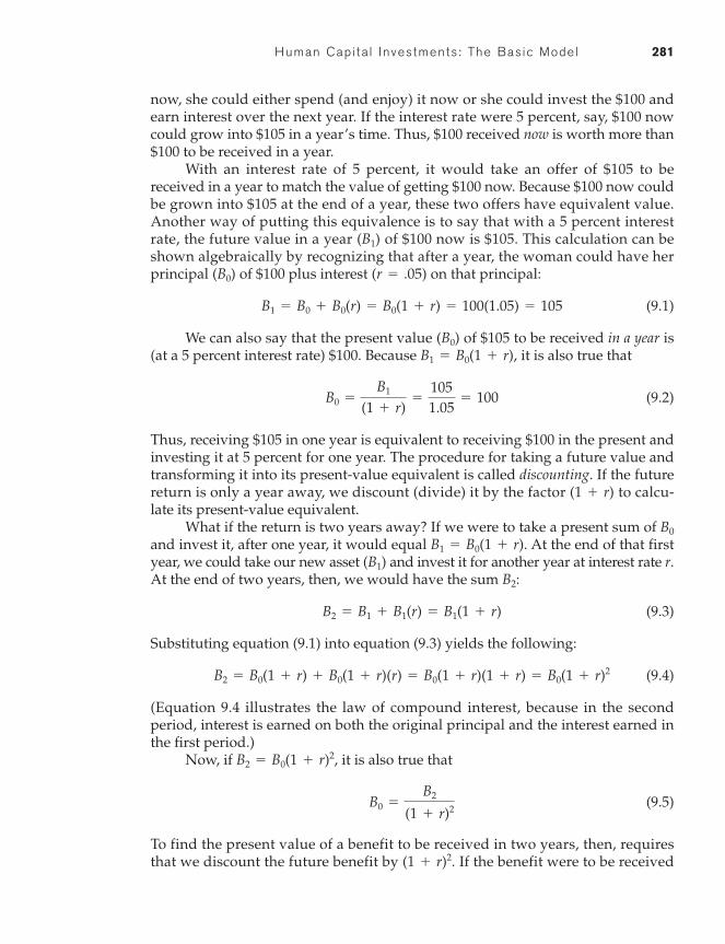
now, she could either spend (and enjoy) it now or she could invest the $100 andearn interest over the next year. If the interest rate were 5 percent, say, $100 nowcould grow into $105 in a year’s time. Thus, $100 received now is worth more than$100 to be received in a year.
With an interest rate of 5 percent, it would take an offer of $105 to bereceived in a year to match the value of getting $100 now. Because $100 now couldbe grown into $105 at the end of a year, these two offers have equivalent value.Another way of putting this equivalence is to say that with a 5 percent interestrate, the future value in a year of $100 now is $105. This calculation can beshown algebraically by recognizing that after a year, the woman could have herprincipal of $100 plus interest on that principal:
(9.1)
We can also say that the present value of $105 to be received in a year is(at a 5 percent interest rate) $100. Because it is also true that
(9.2)
Thus, receiving $105 in one year is equivalent to receiving $100 in the present andinvesting it at 5 percent for one year. The procedure for taking a future value andtransforming it into its present-value equivalent is called discounting. If the futurereturn is only a year away, we discount (divide) it by the factor to calcu-late its present-value equivalent.
What if the return is two years away? If we were to take a present sum of B0and invest it, after one year, it would equal At the end of that firstyear, we could take our new asset and invest it for another year at interest rate r.At the end of two years, then, we would have the sum B2:
(9.3)
Substituting equation (9.1) into equation (9.3) yields the following:
(9.4)
(Equation 9.4 illustrates the law of compound interest, because in the secondperiod, interest is earned on both the original principal and the interest earned inthe first period.)
Now, if it is also true that
(9.5)
To find the present value of a benefit to be received in two years, then, requiresthat we discount the future benefit by If the benefit were to be received(1 + r)2.
B0 =B2
(1 + r)2
B2 = B0(1 + r)2,
B2 = B0(1 + r) + B0(1 + r)(r) = B0(1 + r)(1 + r) = B0(1 + r)2
B2 = B1 + B1(r) = B1(1 + r)
(B1)B1 = B0(1 + r).
(1 + r)
B0 =B1
(1 + r)=
1051.05
= 100
B1 = B0(1 + r),(B0)
B1 = B0 + B0(r) = B0(1 + r) = 100(1.05) = 105
(r = .05)(B0)
(B1)
282 Chapter 9 Investments in Human Capi ta l : Educat ion and Tra in ing
in three years, we can use the logic underlying equations (9.3) and (9.4) to calculatethat the discount factor would be Benefits in four years would be dis-counted to their present values by dividing by and so forth. Clearly,the discount factors rise exponentially, reflecting that current funds can earncompound interest if left invested at interest rate r.
If a human capital investment yields returns of in the first year, in thesecond, and so forth for T years, the sum of these benefits has a present value thatis calculated as follows:
(9.6)
where the interest rate (or discount rate) is r. As long as r is positive, benefits in thefuture will be progressively discounted. For example, if benefits payablein 30 years would receive a weight that is only 17 percent of the weight placed onbenefits payable immediately The smaller r is, thegreater the weight placed on future benefits; for example, if a benefitpayable in 30 years would receive a weight that is 55 percent of the weight givento an immediate benefit.
Modeling the Human Capital Investment DecisionOur model of human capital investment assumes that people are utility maximiz-ers and take a lifetime perspective when making choices about education andtraining. They are therefore assumed to compare the near-term investment costs(C) with the present value of expected future benefits when making a decision,say, about additional schooling. Investment in additional schooling is attractive ifthe present value of future benefits exceeds costs:
(9.7)
Utility maximization, of course, requires that people continue to make additionalhuman capital investments as long as condition (9.7) is met and that they stoponly when the benefits of additional investment are equal to or less than the addi-tional costs.
There are two ways we can measure whether the criterion in equation (9.7)is met. Using the present-value method, we can specify a value for the discount rate,r, and then determine how the present value of benefits compares to costs. Alter-natively, we can adopt the internal rate of return method, which asks, “How largecould the discount rate be and still render the investment profitable?” Clearly, ifthe benefits are so large that even a very high discount rate would render invest-ment profitable, then the project is worthwhile. In practice, we calculate this
B1
1 + r+
B2
(1 + r)2 + Á +BT
(1 + r)T 7 C
r = 0.02,(1.0630 = 5.74; 1>5.74 = 0.17).
r = 0.06,
Present Value =B1
1 + r+
B2
(1 + r)2 +B3
(1 + r)3 + Á +BT
(1 + r)T
B2B1
(1 + r)4,(1 + r)3.
internal rate of return by setting the present value of benefits equal to costs, solvingfor r, and then comparing r to the rate of return on other investments.
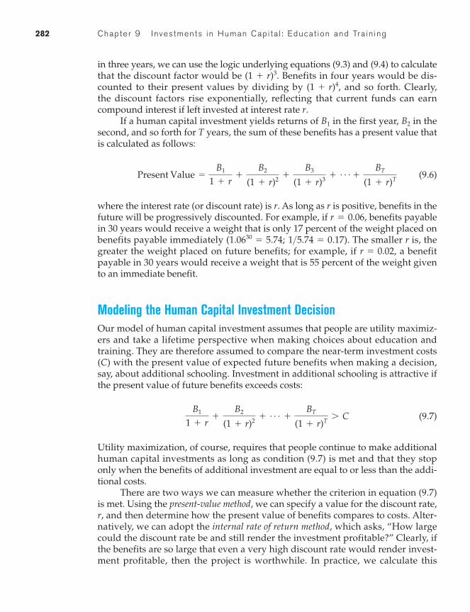
Some basic implications of the model embedded in expression (9.7) are illus-trated graphically in Figure 9.1, which depicts human capital decisions in termsof marginal costs and marginal benefits (focus for now on the black lines in thefigure). The marginal costs (MC) of each additional unit of human capital (thetuition, supplies, forgone earnings, and psychic costs of an additional year ofschooling, say) are assumed to be constant. The present value of the marginal ben-efits (MB) is shown as declining, because each added year of schooling meansfewer years over which benefits can be collected. The utility-maximizing amountof human capital for any individual is shown as that amount for which
Those who find learning to be especially arduous will implicitly attach ahigher marginal psychic cost to acquiring human capital. As shown by the blueline, in Figure 9.1a, individuals with higher MC will acquire lower levels ofhuman capital (compare with ). Similarly, those who expect smallerfuture benefits from additional human capital investments (the blue line, inFigure 9.1b) will acquire less human capital.
This straightforward theory yields some interesting insights about thebehavior and earnings of workers. Many of these insights can be discovered byanalyzing the decision confronting young adults about whether to invest full-timein college after leaving high school.
MB¿,HC*HC¿
MC¿,
MC = MB.(HC*)
Human Capi ta l Investments : The Basic Model 283
0
Marginal Costs (MC)and Benefits (MB)
Units of Human Capital (HC)
MC�
MC
HC*HC�
MB
0
Units of Human Capital (HC)
MC
HC*HC �
MB
MB�
(a) (b)
Figure 9.1
The Optimum Acquisition of Human Capital
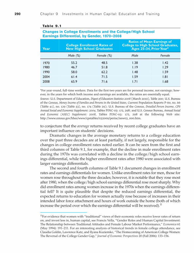
The Demand for a College EducationThe demand for a college education, as measured by the percentage of graduat-ing high school seniors who enroll in college, is surprisingly variable. For males,enrollment rates went from 55.2 percent in 1970, down to 46.7 percent in 1980,back to 58 percent in 1990, and reaching almost 66 percent by 2008. The compara-ble enrollment rates for women started lower, at 48.5 percent in 1970, rose slowlyduring the 1970s, and then have risen quickly thereafter, reaching 71.6 percent by2008. Why have enrollment rates followed these patterns?
Weighing the Costs and Benefits of CollegeClearly, people attend college when they believe they will be better off by sodoing. For some, at least part of the benefits may be short term—they like thecourses or the lifestyle of a student—and to this extent, college is at least partiallya consumption good. The consumption benefits of college, however, are unlikely tochange much over the course of a decade, so changes in college attendance ratesover relatively short periods of time probably reflect changes in MC or benefitsassociated with the investment aspects of college attendance.
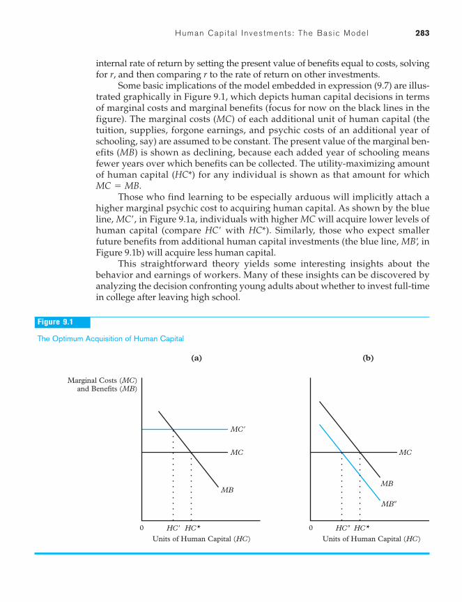
A person considering college has, in some broad sense, a choice betweentwo streams of earnings over his or her lifetime. Stream A begins immediately butdoes not rise very high; it is the earnings stream of a high school graduate. Stream B(the college graduate) has a negative income for the first four years (owing to col-lege tuition costs), followed by a period when the salary may be less than whatthe high school graduate makes, but then it takes off and rises above stream A.Both streams are illustrated in Figure 9.2. (Why these streams are differentially
284 Chapter 9 Investments in Human Capi ta l : Educat ion and Tra in ing
Earnings(dollars)
A
0
B
Age ofWorker
EarningsStream B
EarningsStream A
ForgoneEarnings
Tuition,Books
GrossBenefits
CostOutlays
(dollars)
18 22
Figure 9.2
Alternative EarningsStreams
The Demand for a Col lege Educat ion 285
curved will be discussed later in this chapter.) The streams shown in the figure arestylized so that we can emphasize some basic points. Actual earnings streams willbe shown in Figures 9.3 and 9.4.
Obviously, the earnings of the college graduate would have to rise abovethose of the high school graduate to induce someone to invest in a college educa-tion (unless, of course, the consumption-related returns were large). The grossbenefits—the difference in earnings between the two streams—must total muchmore than the costs because such returns are in the future and are therefore dis-counted. For example, suppose it costs $25,000 per year to obtain a four-year col-lege education and the real interest rate (the nominal rate less the rate of inflation)is 2 percent. The after-tax returns—if they were the same each year—must be$3,652 in constant-dollar terms (that is, after taking away the effects of inflation)each year for 40 years in order to justify the investment on purely monetarygrounds. These returns must be $3,652 because $100,000 invested at a 2 percentinterest rate can provide a payment (of interest and principal) totaling $3,652 ayear for 40 years.2
Predictions of the TheoryIn deciding whether to attend college, no doubt few students make the very pre-cise calculations suggested in expression (9.7). Nevertheless, if they make less for-mal estimates that take into account the same factors, we can make fourpredictions concerning the demand for college education:
1. Present-oriented people are less likely to go to college than forward-looking people (other things equal).
2. Most college students will be young.3. College attendance will decrease if the costs of college rise (other things
equal).4. College attendance will increase if the gap between the earnings of col-
lege graduates and high school graduates widens (again, other thingsequal).
Present-Orientedness Although we all discount the future somewhat withrespect to the present, psychologists use the term present-oriented to describe people who do not weight future events or outcomes very heavily. In terms of
2This calculation is made using the annuity formula:
where the total investment ($100,000 in our example), the yearly payment ($3,652), the rateof interest (0.02), and the number of years (40). In this example, we treat the costs of a college edu-cation as being incurred all in one year rather than being spread out over four, a simplification thatdoes not alter the magnitude of required returns much at all.
n =r =X =Y =
Y = X1 - [1>11 + r2n]
r
286 Chapter 9 Investments in Human Capi ta l : Educat ion and Tra in ing
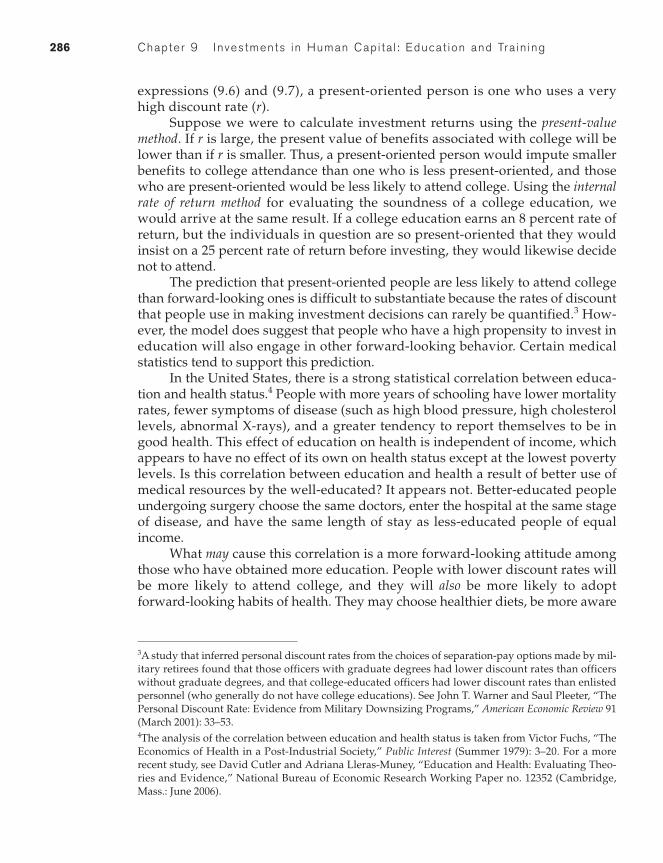
expressions (9.6) and (9.7), a present-oriented person is one who uses a veryhigh discount rate (r).
Suppose we were to calculate investment returns using the present-valuemethod. If r is large, the present value of benefits associated with college will belower than if r is smaller. Thus, a present-oriented person would impute smallerbenefits to college attendance than one who is less present-oriented, and thosewho are present-oriented would be less likely to attend college. Using the internalrate of return method for evaluating the soundness of a college education, wewould arrive at the same result. If a college education earns an 8 percent rate ofreturn, but the individuals in question are so present-oriented that they wouldinsist on a 25 percent rate of return before investing, they would likewise decidenot to attend.
The prediction that present-oriented people are less likely to attend collegethan forward-looking ones is difficult to substantiate because the rates of discountthat people use in making investment decisions can rarely be quantified.3 How-ever, the model does suggest that people who have a high propensity to invest ineducation will also engage in other forward-looking behavior. Certain medicalstatistics tend to support this prediction.
In the United States, there is a strong statistical correlation between educa-tion and health status.4 People with more years of schooling have lower mortalityrates, fewer symptoms of disease (such as high blood pressure, high cholesterollevels, abnormal X-rays), and a greater tendency to report themselves to be ingood health. This effect of education on health is independent of income, whichappears to have no effect of its own on health status except at the lowest povertylevels. Is this correlation between education and health a result of better use ofmedical resources by the well-educated? It appears not. Better-educated peopleundergoing surgery choose the same doctors, enter the hospital at the same stageof disease, and have the same length of stay as less-educated people of equalincome.
What may cause this correlation is a more forward-looking attitude amongthose who have obtained more education. People with lower discount rates willbe more likely to attend college, and they will also be more likely to adopt forward-looking habits of health. They may choose healthier diets, be more aware
3A study that inferred personal discount rates from the choices of separation-pay options made by mil-itary retirees found that those officers with graduate degrees had lower discount rates than officerswithout graduate degrees, and that college-educated officers had lower discount rates than enlistedpersonnel (who generally do not have college educations). See John T. Warner and Saul Pleeter, “ThePersonal Discount Rate: Evidence from Military Downsizing Programs,” American Economic Review 91(March 2001): 33–53.4The analysis of the correlation between education and health status is taken from Victor Fuchs, “TheEconomics of Health in a Post-Industrial Society,” Public Interest (Summer 1979): 3–20. For a morerecent study, see David Cutler and Adriana Lleras-Muney, “Education and Health: Evaluating Theo-ries and Evidence,” National Bureau of Economic Research Working Paper no. 12352 (Cambridge,Mass.: June 2006).
The Demand for a Col lege Educat ion 287
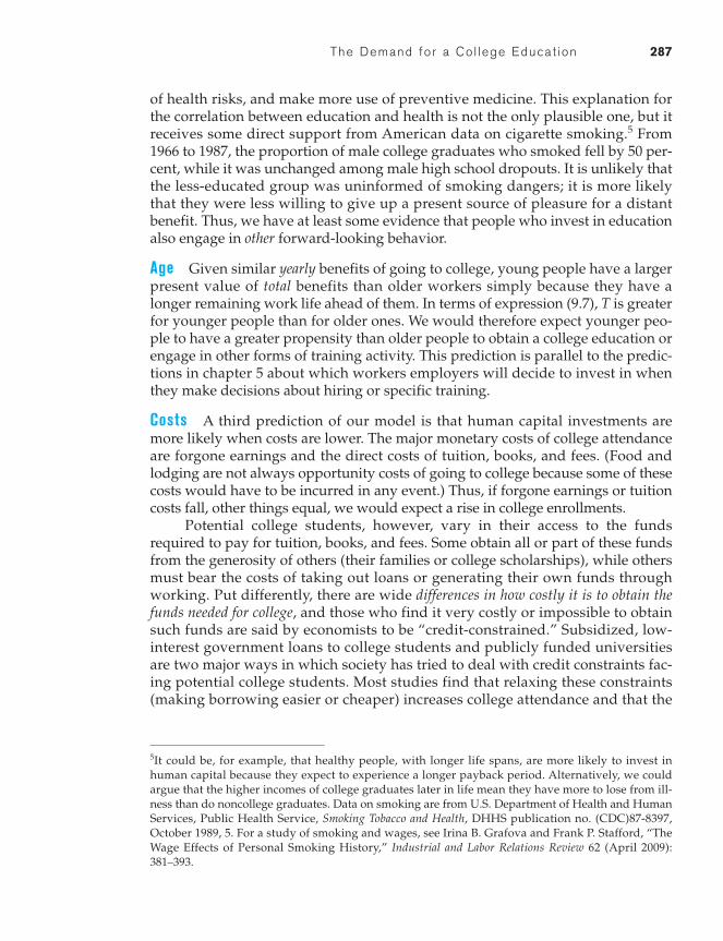
of health risks, and make more use of preventive medicine. This explanation forthe correlation between education and health is not the only plausible one, but itreceives some direct support from American data on cigarette smoking.5 From1966 to 1987, the proportion of male college graduates who smoked fell by 50 per-cent, while it was unchanged among male high school dropouts. It is unlikely thatthe less-educated group was uninformed of smoking dangers; it is more likelythat they were less willing to give up a present source of pleasure for a distantbenefit. Thus, we have at least some evidence that people who invest in educationalso engage in other forward-looking behavior.
Age Given similar yearly benefits of going to college, young people have a largerpresent value of total benefits than older workers simply because they have alonger remaining work life ahead of them. In terms of expression (9.7), T is greaterfor younger people than for older ones. We would therefore expect younger peo-ple to have a greater propensity than older people to obtain a college education orengage in other forms of training activity. This prediction is parallel to the predic-tions in chapter 5 about which workers employers will decide to invest in whenthey make decisions about hiring or specific training.
Costs A third prediction of our model is that human capital investments aremore likely when costs are lower. The major monetary costs of college attendanceare forgone earnings and the direct costs of tuition, books, and fees. (Food andlodging are not always opportunity costs of going to college because some of thesecosts would have to be incurred in any event.) Thus, if forgone earnings or tuitioncosts fall, other things equal, we would expect a rise in college enrollments.
Potential college students, however, vary in their access to the fundsrequired to pay for tuition, books, and fees. Some obtain all or part of these fundsfrom the generosity of others (their families or college scholarships), while othersmust bear the costs of taking out loans or generating their own funds throughworking. Put differently, there are wide differences in how costly it is to obtain thefunds needed for college, and those who find it very costly or impossible to obtainsuch funds are said by economists to be “credit-constrained.” Subsidized, low-interest government loans to college students and publicly funded universitiesare two major ways in which society has tried to deal with credit constraints fac-ing potential college students. Most studies find that relaxing these constraints(making borrowing easier or cheaper) increases college attendance and that the
5It could be, for example, that healthy people, with longer life spans, are more likely to invest inhuman capital because they expect to experience a longer payback period. Alternatively, we couldargue that the higher incomes of college graduates later in life mean they have more to lose from ill-ness than do noncollege graduates. Data on smoking are from U.S. Department of Health and HumanServices, Public Health Service, Smoking Tobacco and Health, DHHS publication no. (CDC)87-8397,October 1989, 5. For a study of smoking and wages, see Irina B. Grafova and Frank P. Stafford, “TheWage Effects of Personal Smoking History,” Industrial and Labor Relations Review 62 (April 2009):381–393.
288 Chapter 9 Investments in Human Capi ta l : Educat ion and Tra in ing
public policies undertaken in the United States to relax the constraints have beenlargely successful.6
The costs of college attendance are an additional reason older people are lesslikely to attend than younger ones. As workers age, their greater experience andmaturity result in higher wages and therefore greater opportunity costs of collegeattendance. Interestingly, as suggested by Example 9.2, however, college attendance
6For a recent study that refers to prior literature, see Katharine G. Abraham and Melissa A. Clark,“Financial Aid and Students’ College Decisions: Evidence from the District of Columbia’s TuitionAssistance Grant Program,” Journal of Human Resources 41 (Summer 2006): 578–610. Articles directlymeasuring credit constraints include Stephen V. Cameron and Christopher Taber, “Estimation of Edu-cational Borrowing Constraints Using Returns to Schooling,” Journal of Political Economy 112 (February2004): 132–183; and Pedro Carneiro and James J. Heckman, “The Evidence on Credit Constraints inPost-Secondary Schooling,” Economic Journal 112 (October 2002): 705–734. The latter article analyzesreasons why family income and college attendance rates are positively correlated; it concludes thatfinancial credit constraints are much less important in explaining this relationship than are the atti-tudes and skills children acquire from their parents.
EXAM PLE 9.2
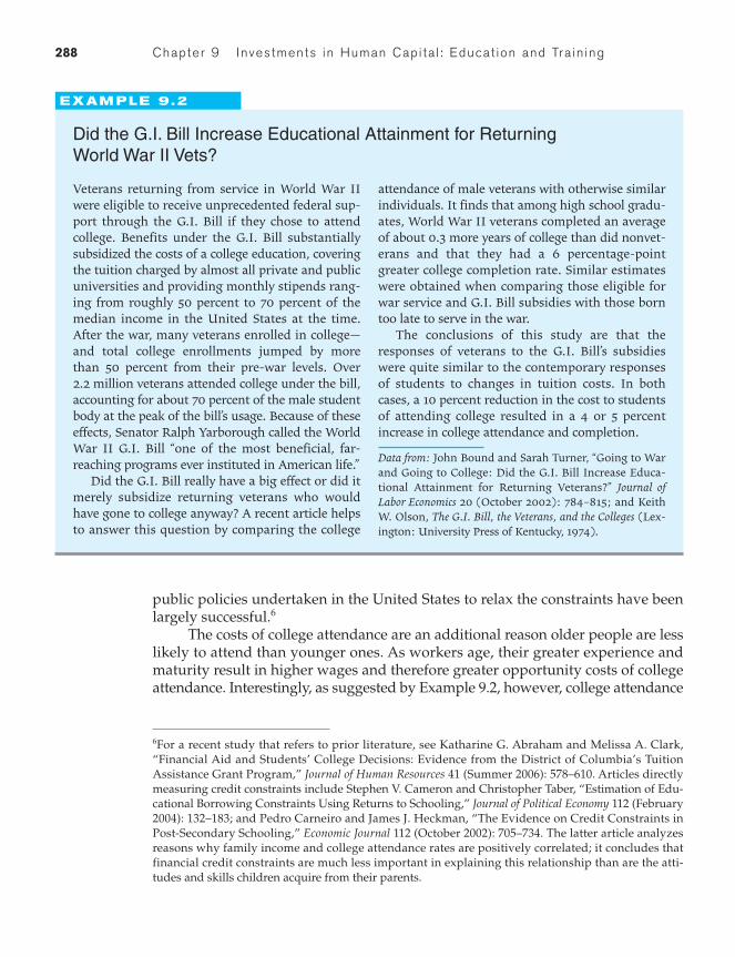
Did the G.I. Bill Increase Educational Attainment for Returning World War II Vets?
Veterans returning from service in World War IIwere eligible to receive unprecedented federal sup-port through the G.I. Bill if they chose to attendcollege. Benefits under the G.I. Bill substantiallysubsidized the costs of a college education, coveringthe tuition charged by almost all private and publicuniversities and providing monthly stipends rang-ing from roughly 50 percent to 70 percent of themedian income in the United States at the time.After the war, many veterans enrolled in college—and total college enrollments jumped by morethan 50 percent from their pre-war levels. Over2.2 million veterans attended college under the bill,accounting for about 70 percent of the male studentbody at the peak of the bill’s usage. Because of theseeffects, Senator Ralph Yarborough called the WorldWar II G.I. Bill “one of the most beneficial, far-reaching programs ever instituted in American life.”
Did the G.I. Bill really have a big effect or did itmerely subsidize returning veterans who wouldhave gone to college anyway? A recent article helpsto answer this question by comparing the college
attendance of male veterans with otherwise similarindividuals. It finds that among high school gradu-ates, World War II veterans completed an averageof about 0.3 more years of college than did nonvet-erans and that they had a 6 percentage-pointgreater college completion rate. Similar estimateswere obtained when comparing those eligible forwar service and G.I. Bill subsidies with those borntoo late to serve in the war.
The conclusions of this study are that theresponses of veterans to the G.I. Bill’s subsidieswere quite similar to the contemporary responsesof students to changes in tuition costs. In bothcases, a 10 percent reduction in the cost to studentsof attending college resulted in a 4 or 5 percentincrease in college attendance and completion.
Data from: John Bound and Sarah Turner, “Going to Warand Going to College: Did the G.I. Bill Increase Educa-tional Attainment for Returning Veterans?” Journal ofLabor Economics 20 (October 2002): 784–815; and KeithW. Olson, The G.I. Bill, the Veterans, and the Colleges (Lex-ington: University Press of Kentucky, 1974).
The Demand for a Col lege Educat ion 289
by military veterans (who are older than the typical college student) has beenresponsive to the educational subsidies for which they are eligible.7
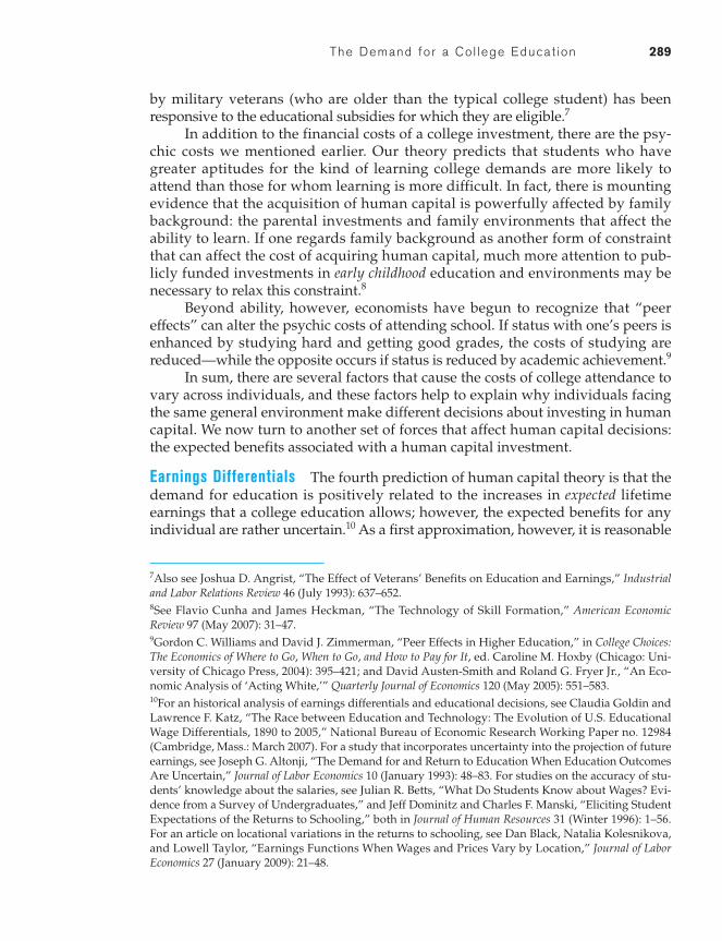
In addition to the financial costs of a college investment, there are the psy-chic costs we mentioned earlier. Our theory predicts that students who havegreater aptitudes for the kind of learning college demands are more likely toattend than those for whom learning is more difficult. In fact, there is mountingevidence that the acquisition of human capital is powerfully affected by familybackground: the parental investments and family environments that affect theability to learn. If one regards family background as another form of constraintthat can affect the cost of acquiring human capital, much more attention to pub-licly funded investments in early childhood education and environments may benecessary to relax this constraint.8
Beyond ability, however, economists have begun to recognize that “peereffects” can alter the psychic costs of attending school. If status with one’s peers isenhanced by studying hard and getting good grades, the costs of studying arereduced—while the opposite occurs if status is reduced by academic achievement.9
In sum, there are several factors that cause the costs of college attendance tovary across individuals, and these factors help to explain why individuals facingthe same general environment make different decisions about investing in humancapital. We now turn to another set of forces that affect human capital decisions:the expected benefits associated with a human capital investment.
Earnings Differentials The fourth prediction of human capital theory is that thedemand for education is positively related to the increases in expected lifetimeearnings that a college education allows; however, the expected benefits for anyindividual are rather uncertain.10 As a first approximation, however, it is reasonable
7Also see Joshua D. Angrist, “The Effect of Veterans’ Benefits on Education and Earnings,” Industrialand Labor Relations Review 46 (July 1993): 637–652.8See Flavio Cunha and James Heckman, “The Technology of Skill Formation,” American EconomicReview 97 (May 2007): 31–47.9Gordon C. Williams and David J. Zimmerman, “Peer Effects in Higher Education,” in College Choices:The Economics of Where to Go, When to Go, and How to Pay for It, ed. Caroline M. Hoxby (Chicago: Uni-versity of Chicago Press, 2004): 395–421; and David Austen-Smith and Roland G. Fryer Jr., “An Eco-nomic Analysis of ‘Acting White,’” Quarterly Journal of Economics 120 (May 2005): 551–583.10For an historical analysis of earnings differentials and educational decisions, see Claudia Goldin andLawrence F. Katz, “The Race between Education and Technology: The Evolution of U.S. EducationalWage Differentials, 1890 to 2005,” National Bureau of Economic Research Working Paper no. 12984(Cambridge, Mass.: March 2007). For a study that incorporates uncertainty into the projection of futureearnings, see Joseph G. Altonji, “The Demand for and Return to Education When Education OutcomesAre Uncertain,” Journal of Labor Economics 10 (January 1993): 48–83. For studies on the accuracy of stu-dents’ knowledge about the salaries, see Julian R. Betts, “What Do Students Know about Wages? Evi-dence from a Survey of Undergraduates,” and Jeff Dominitz and Charles F. Manski, “Eliciting StudentExpectations of the Returns to Schooling,” both in Journal of Human Resources 31 (Winter 1996): 1–56.For an article on locational variations in the returns to schooling, see Dan Black, Natalia Kolesnikova,and Lowell Taylor, “Earnings Functions When Wages and Prices Vary by Location,” Journal of LaborEconomics 27 (January 2009): 21–48.
Tab le 9 .1
Changes in College Enrollments and the College/High SchoolEarnings Differential, by Gender, 1970–2008
YearCollege Enrollment Rates ofNew High School Graduates
Ratios of Mean Earnings ofCollege to High School Graduates,
Ages 25–34, Prior Yeara
Male (%) Female (%) Male Female
1970 55.2 48.5 1.38 1.421980 46.7 51.8 1.19 1.291990 58.0 62.2 1.48 1.592004 61.4 71.5 1.59 1.812008 65.9 71.6 1.71 1.68
aFor year-round, full-time workers. Data for the first two years are for personal income, not earnings; how-ever, in the years for which both income and earnings are available, the ratios are essentially equal.Sources: U.S. Department of Education, Digest of Education Statistics 2008 (March 2010), Table 200; U.S. Bureauof the Census, Money Income of Families and Persons in the United States, Current Population Reports P-60, no. 66(Table 41), no. 129 (Table 53), no. 174 (Table 29); U.S. Bureau of the Census, Detailed Person Income, CPSAnnual Social and Economic Supplement: 2004, Tables PINC-03: 172, 298; and U.S. Census Bureau, Annual Socialand Economic (ASEC) Supplement: 2008, Tables PINC-03: 172, 298 at the following Web site:http://www.census.gov/hhes/www/cpstables/032009/perinc/new03_000.htm.
290 Chapter 9 Investments in Human Capi ta l : Educat ion and Tra in ing
to conjecture that the average returns received by recent college graduates have animportant influence on students’ decisions.
Dramatic changes in the average monetary returns to a college educationover the past three decades are at least partially, if not largely, responsible for thechanges in college enrollment rates noted earlier. It can be seen from the first andthird columns of Table 9.1, for example, that the decline in male enrollment ratesduring the 1970s was correlated with a decline in the college/high school earn-ings differential, while the higher enrollment rates after 1980 were associated withlarger earnings differentials.
The second and fourth columns of Table 9.1 document changes in enrollmentrates and earnings differentials for women. Unlike enrollment rates for men, those forwomen rose throughout the three decades; however, it is notable that they rose mostafter 1980, when the college/high school earnings differential rose most sharply. Whydid enrollment rates among women increase in the 1970s when the earnings differen-tial fell? It is quite plausible that despite the reduced earnings differential, theexpected returns to education for women actually rose because of increases in theirintended labor force attachment and hours of work outside the home (both of whichincrease the period over which the earnings differential will be received).11
11For evidence that women with “traditional” views of their economic roles receive lower rates of returnon, and invest less in, human capital, see Francis Vella, “Gender Roles and Human Capital Investment:The Relationship between Traditional Attitudes and Female Labour Market Performance,” Economica 61(May 1994): 191–211. For an interesting analysis of historical trends in female college attendance, seeClaudia Goldin, Lawrence Katz, and Ilyana Kuziemko, “The Homecoming of American College Women:The Reversal of the College Gender Gap,” Journal of Economic Perspectives 20 (Fall 2006): 133–156.
The Demand for a Col lege Educat ion 291
It is important to recognize that human capital investments, like otherinvestments, entail uncertainty. While it is helpful for individuals to know theaverage earnings differentials between college and high school graduates, theymust also assess their own probabilities of success in specific fields requiring acollege degree. If, for example, the average returns to college are rising, butthere is a growing spread between the earnings of the most successful collegegraduates and the least successful ones, individuals who believe they arelikely to be in the latter group may be deterred from making an investment incollege. Recent studies have pointed to the importance of friends, ethnic affili-ation, and neighborhoods in the human capital decisions of individuals, evenafter controlling for the effects of parental income or education. While thesepeer effects can affect educational decisions by affecting costs, as discussedearlier, it is also likely that the presence of role models helps to reduce theuncertainty that inevitably surrounds estimates of future success in specificareas.12
Market Responses to Changes in College AttendanceLike other market prices, the returns to college attendance are determined by theforces of both employer demand and employee supply. If more high school stu-dents decide to attend college when presented with higher returns to such aninvestment, market forces are put into play that will tend to lower these returnsin the future. Increased numbers of college graduates put downward pressure onthe wages observed in labor markets for these graduates, other things equal,while a fall in the number of high school graduates will tend to raise wages inmarkets for less-educated workers.
Thus, adding to uncertainties about expected payoffs to an investment incollege is the fact that current returns may be an unreliable estimate of futurereturns. A high return now might motivate an individual to opt for college, but itwill also cause many others to do likewise. An influx of college graduates in fouryears could put downward pressure on returns at that time, which reminds usthat all investments—even human capital ones—involve outlays now and uncer-tain returns in the future. (For an analysis of how the labor market might respondwhen workers behave as if the returns observed currently will persist into thefuture, see Appendix 9A.)
12For papers on the issues discussed in this paragraph, see Kerwin Kofi Charles and Ming-ChingLuoh, “Gender Differences in Completed Schooling,” Review of Economics and Statistics 85 (August2003): 559–577; Ira N. Gang and Klaus F. Zimmermann, “Is Child Like Parent? Educational Attainmentand Ethnic Origin,” Journal of Human Resources 35 (Summer 2000): 550–569; and Eric Maurin and San-dra McNally, “Vive la Révolution! Long-Term Educational Returns of 1968 to the Angry Students,”Journal of Labor Economics (January 2008): 1–33.

Education, Earnings, and Post-SchoolingInvestments in Human Capital
The preceding section used human capital theory to analyze the decision toundertake a formal educational program (college) on a full-time basis. We nowturn to an analysis of workers’ decisions to acquire training at work. The presenceof on-the-job training is difficult for the economist to directly observe; much of itis informal and not publicly recorded. We can, however, use human capital the-ory and certain patterns in workers’ lifetime earnings to draw inferences abouttheir demand for this type of training.
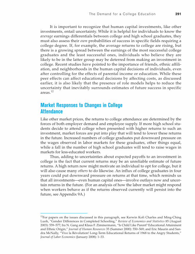
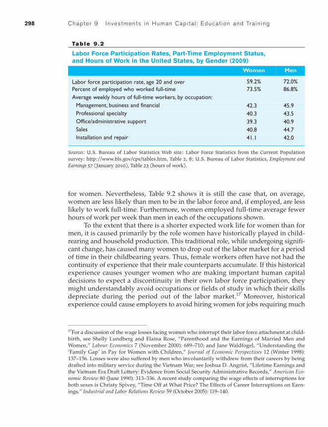
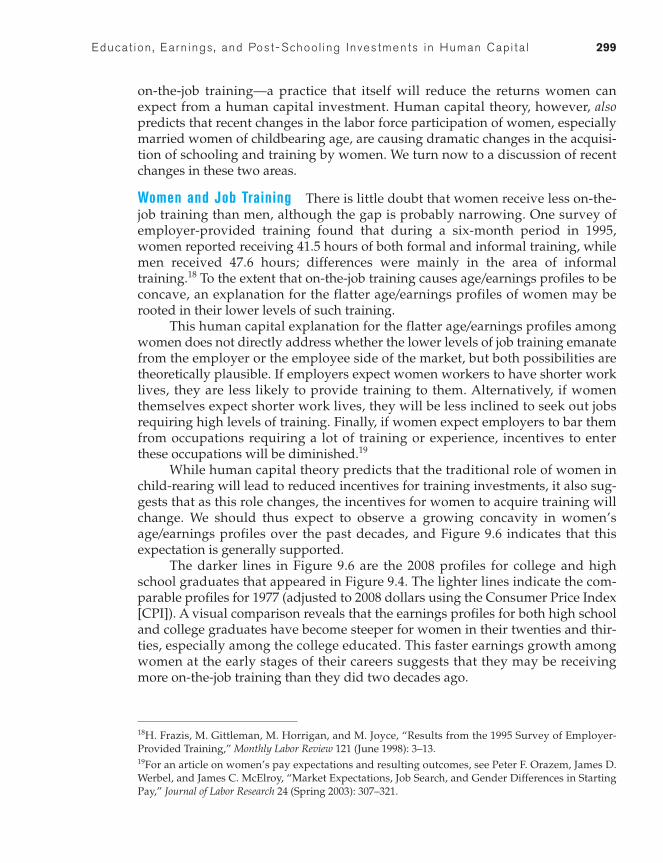
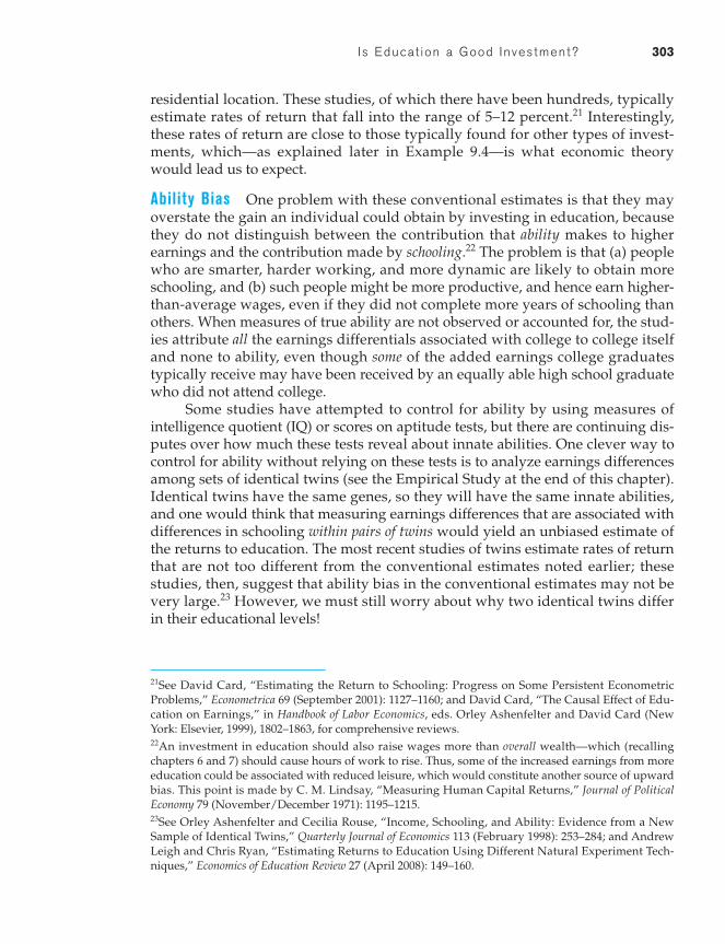
Figures 9.3 and 9.4 graph the 2008 earnings of men and women of various ages with different levels of education. These figures reveal four notable characteristics:
1. Average earnings of full-time workers rise with the level of education.
2. The most rapid increase in earnings occurs early, thus giving a concaveshape to the age/earnings profiles of both men and women.
3. Age/earnings profiles tend to fan out, so that education-related earningsdifferences later in workers’ lives are greater than those early on.
4. The age/earnings profiles of men tend to be more concave and to fan outmore than those for women.
Can human capital theory help explain the above empirical regularities?
Average Earnings and Educational LevelOur investment model of educational choice implies that earnings rise with thelevel of education, for if they did not, the incentives for students to invest in moreeducation would disappear. It is thus not too surprising to see in Figures 9.3 and9.4 that the average earnings of more-educated workers exceed those of less-educated workers.
Remember, however, that earnings are influenced by both wage rates andhours of work. Data on wage rates are probably most relevant when we look at thereturns to an educational investment, because they indicate pay per unit of timeat work. Wage data, however, are less widely available than earnings data. A crude, but readily available, way to control for working hours when using earn-ings data is to focus on full-time, year-round workers—which we do in Figures 9.3and 9.4. More careful statistical analyses, however, which control for hours ofwork and factors other than education that can increase wage rates, come to thesame conclusion suggested by Figures 9.3 and 9.4: namely, that more education isassociated with higher pay.
292 Chapter 9 Investments in Human Capi ta l : Educat ion and Tra in ing

Educat ion , Earn ings , and Post- School ing Investments in Human Capi ta l 293
10
15
20
25
30
35
40
45
50
55
21 27 32 37 42 47 52
Age
Earningsper year
(in thousands)
College Graduate
60
65
70
75
80
85
90
95
100
Some High School
High School Graduate
Some College
Figure 9.3
Money Earnings (Mean) forFull-Time, Year-Round MaleWorkers, 2008
Source: See footnote 13.
294 Chapter 9 Investments in Human Capi ta l : Educat ion and Tra in ing
On-the-Job Training and the Concavity of Age/Earnings ProfilesThe age/earnings profiles in Figures 9.3 and 9.4 typically rise steeply early on, thentend to flatten.13 While in chapters 10 and 11 we will encounter other potential
10
15
20
25
30
35
40
45
50
55
60
65
21 27 32 37 42 47 52
Age
Earningsper year
(in thousands)
College Graduate
Some High School
High School Graduate
Some College
Figure 9.4
Money Earnings (Mean) forFull-Time, Year-RoundFemale Workers, 2008
Source: See footnote 13.
13Data in these figures are from the U.S. Bureau of the Census Web site: http://www.census.gov/hhes/www/cpstables/032009/perinc/new03_172.htm (males) and http://www.census.gov/hhes/www/cpstables/032009/perinc/new03_298.htm (females). These data match average earnings with age and edu-cation in a given year and do not follow individuals through time. For a paper using longitudinal data onindividuals, see Richard W. Johnson and David Neumark, “Wage Declines and Older Men,” Review of Eco-nomics and Statistics 78 (November 1996): 740–748; for a paper that follows cohorts of individuals throughtime, see David Card and Thomas Lemieux, “Can Falling Supply Explain the Rising Return to College forYounger Men? A Cohort-Based Approach,” Quarterly Journal of Economics 116 (May 2001): 705–746.
Educat ion , Earn ings , and Post- School ing Investments in Human Capi ta l 295
explanations for why earnings rise in this way with age, human capital theoryexplains the concavity of these profiles in terms of on-the-job training.14
Training Declines with Age Training on the job can occur through learning bydoing (skills improving with practice), through formal training programs at oraway from the workplace, or by informally working under the tutelage of a moreexperienced worker. All forms entail reduced productivity among trainees duringthe learning process, and both formal and informal training also involve a com-mitment of time by those who serve as trainers or mentors. Training costs areeither shared by workers and the employer, as with specific training, or are bornemostly by the employee (in the case of general training).
From the perspective of workers, training depresses wages during the learn-ing period but allows them to rise with enhanced productivity afterward. Thus,workers who opt for jobs that require a training investment are willing to acceptlower wages in the short run to get higher pay later on. As with other human cap-ital investments, returns are generally larger when the post-investment period islonger, so we would expect workers’ investments in on-the-job training to begreatest at younger ages and to fall gradually as they grow older.
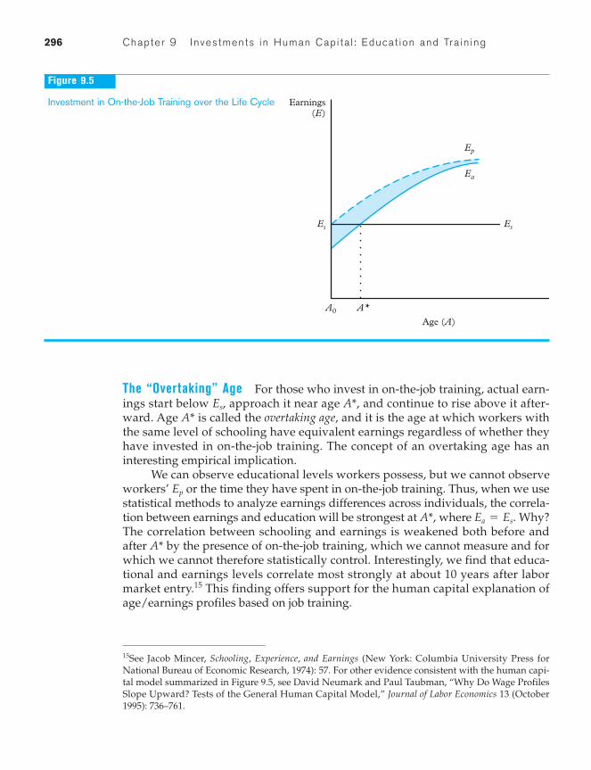
Figure 9.5 graphically depicts the life cycle implications of human capitaltheory as it applies to on-the-job training. The individual depicted has completedfull-time schooling and is able to earn at age Without further training, ifthe knowledge and skills the worker possesses do not depreciate over time, earn-ings would remain at over the life cycle. If the worker chooses to invest in on-the-job training, his or her future earnings potential can be enhanced, asshown by the (dashed) curve in the figure. Investment in on-the-job training,however, has the near-term consequence that actual earnings are below poten-tial; thus, in terms of Figure 9.5, actual earnings lie below as long as theworker is investing. In fact, the gap between and equals the worker’sinvestment costs.
Figure 9.5 is drawn to reflect the theoretical implication, noted earlier, thathuman capital investments decline with age. With each succeeding year, actualearnings become closer to potential earnings; furthermore, because workersbecome less willing to invest in human capital as they age, the yearly increases inpotential earnings become smaller and smaller. Thus, curve takes on a concaveshape, quickly rising above but flattening later in the life cycle. Curve (whichis what we observe in Figures 9.3 and 9.4) takes on its concave shape for the samereasons.
EaEs
Ep
EaEp
Ep(Ea)
Ep
Es
A0.Es
14For discussions of the relative importance of the human capital explanation for rising age/earningsprofiles, see Ann P. Bartel, “Training, Wage Growth, and Job Performance: Evidence from a CompanyDatabase,” Journal of Labor Economics 13 (July 1995): 401–425; Charles Brown, “Empirical Evidence onPrivate Training,” in Research in Labor Economics, vol. 11, eds. Lauri J. Bassi and David L. Crawford(Greenwich, Conn.: JAI Press, 1990): 97–114; and Jacob Mincer, “The Production of Human Capital andthe Life Cycle of Earnings: Variations on a Theme,” Journal of Labor Economics 15, no. 1, pt. 2 (January1997): S26–S47.
296 Chapter 9 Investments in Human Capi ta l : Educat ion and Tra in ing
The “Overtaking” Age For those who invest in on-the-job training, actual earn-ings start below approach it near age and continue to rise above it after-ward. Age is called the overtaking age, and it is the age at which workers withthe same level of schooling have equivalent earnings regardless of whether theyhave invested in on-the-job training. The concept of an overtaking age has aninteresting empirical implication.
We can observe educational levels workers possess, but we cannot observeworkers’ or the time they have spent in on-the-job training. Thus, when we usestatistical methods to analyze earnings differences across individuals, the correla-tion between earnings and education will be strongest at where Why?The correlation between schooling and earnings is weakened both before andafter by the presence of on-the-job training, which we cannot measure and forwhich we cannot therefore statistically control. Interestingly, we find that educa-tional and earnings levels correlate most strongly at about 10 years after labormarket entry.15 This finding offers support for the human capital explanation ofage/earnings profiles based on job training.
A*
Ea = Es.A*,
Ep
A*A*,Es,
A0
Earnings(E)
Age (A)
Es Es
Ep
Ea
A*
Figure 9.5
Investment in On-the-Job Training over the Life Cycle
15See Jacob Mincer, Schooling, Experience, and Earnings (New York: Columbia University Press forNational Bureau of Economic Research, 1974): 57. For other evidence consistent with the human capi-tal model summarized in Figure 9.5, see David Neumark and Paul Taubman, “Why Do Wage ProfilesSlope Upward? Tests of the General Human Capital Model,” Journal of Labor Economics 13 (October1995): 736–761.
Educat ion , Earn ings , and Post- School ing Investments in Human Capi ta l 297
The Fanning Out of Age/Earnings ProfilesEarnings differences across workers with different educational backgrounds tendto become more pronounced as they age. This phenomenon is also consistent withwhat human capital theory would predict.
Investments in human capital tend to be more likely when the expectedearnings differentials are greater, when the initial investment costs are lower, andwhen the investor has either a longer time to recoup the returns or a lower dis-count rate. The same can be said of people who have the ability to learn morequickly. The ability to learn rapidly shortens the training period, and fast learnersprobably also experience lower psychic costs (lower levels of frustration) duringtraining.
Thus, people who have the ability to learn quickly are those most likely toseek out—and be presented by employers with—training opportunities. But whoare these fast learners? They are most likely the people who, because of their abili-ties, were best able to reap benefits from formal schooling! Thus, human capitaltheory leads us to expect that workers who invested more in schooling will alsoinvest more in post-schooling job training.16
The tendency of the better-educated workers to invest more in job trainingexplains why their age/earnings profiles start low, rise quickly, and keep risingafter the profiles of their less-educated counterparts have leveled off. Their earn-ings rise more quickly because they are investing more heavily in job training,and they rise for a longer time for the same reason. In other words, people withthe ability to learn quickly select the ultimately high-paying jobs where muchlearning is required and thus put their abilities to greatest advantage.
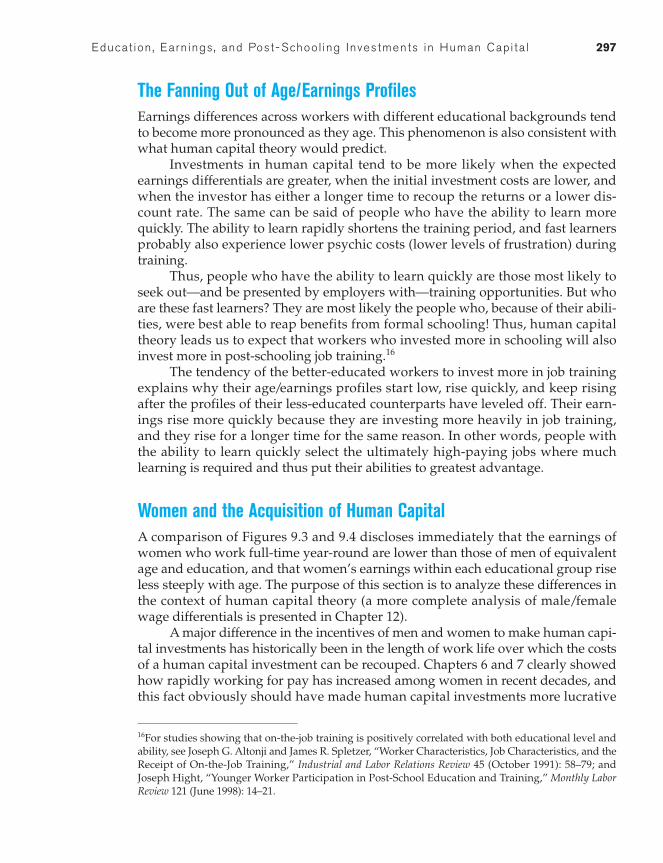
Women and the Acquisition of Human CapitalA comparison of Figures 9.3 and 9.4 discloses immediately that the earnings ofwomen who work full-time year-round are lower than those of men of equivalentage and education, and that women’s earnings within each educational group riseless steeply with age. The purpose of this section is to analyze these differences inthe context of human capital theory (a more complete analysis of male/femalewage differentials is presented in Chapter 12).
A major difference in the incentives of men and women to make human capi-tal investments has historically been in the length of work life over which the costsof a human capital investment can be recouped. Chapters 6 and 7 clearly showedhow rapidly working for pay has increased among women in recent decades, andthis fact obviously should have made human capital investments more lucrative
16For studies showing that on-the-job training is positively correlated with both educational level andability, see Joseph G. Altonji and James R. Spletzer, “Worker Characteristics, Job Characteristics, and theReceipt of On-the-Job Training,” Industrial and Labor Relations Review 45 (October 1991): 58–79; andJoseph Hight, “Younger Worker Participation in Post-School Education and Training,” Monthly LaborReview 121 (June 1998): 14–21.
298 Chapter 9 Investments in Human Capi ta l : Educat ion and Tra in ing
for women. Nevertheless, Table 9.2 shows it is still the case that, on average,women are less likely than men to be in the labor force and, if employed, are lesslikely to work full-time. Furthermore, women employed full-time average fewerhours of work per week than men in each of the occupations shown.
To the extent that there is a shorter expected work life for women than formen, it is caused primarily by the role women have historically played in child-rearing and household production. This traditional role, while undergoing signifi-cant change, has caused many women to drop out of the labor market for a periodof time in their childbearing years. Thus, female workers often have not had thecontinuity of experience that their male counterparts accumulate. If this historicalexperience causes younger women who are making important human capitaldecisions to expect a discontinuity in their own labor force participation, theymight understandably avoid occupations or fields of study in which their skillsdepreciate during the period out of the labor market.17 Moreover, historical experience could cause employers to avoid hiring women for jobs requiring much
Tab le 9 .2
Labor Force Participation Rates, Part-Time Employment Status, and Hours of Work in the United States, by Gender (2009)
Women Men
Labor force participation rate, age 20 and over 59.2% 72.0%Percent of employed who worked full-time 73.5% 86.8%Average weekly hours of full-time workers, by occupation:
Management, business and financial 42.3 45.9Professional specialty 40.3 43.5Office/administrative support 39.3 40.9Sales 40.8 44.7Installation and repair 41.1 42.0
Sources: U.S. Bureau of Labor Statistics Web site: Labor Force Statistics from the Current Populationsurvey: http://www.bls.gov/cps/tables.htm, Table 2, 8; U.S. Bureau of Labor Statistics, Employment andEarnings 57 (January 2010), Table 23 (hours of work).
17For a discussion of the wage losses facing women who interrupt their labor force attachment at child-birth, see Shelly Lundberg and Elaina Rose, “Parenthood and the Earnings of Married Men andWomen,” Labour Economics 7 (November 2000): 689–710; and Jane Waldfogel, “Understanding the‘Family Gap’ in Pay for Women with Children,” Journal of Economic Perspectives 12 (Winter 1998):137–156. Losses were also suffered by men who involuntarily withdrew from their careers by beingdrafted into military service during the Vietnam War; see Joshua D. Angrist, “Lifetime Earnings andthe Vietnam Era Draft Lottery: Evidence from Social Security Administrative Records,” American Eco-nomic Review 80 (June 1990): 313–336. A recent study comparing the wage effects of interruptions forboth sexes is Christy Spivey, “Time Off at What Price? The Effects of Career Interruptions on Earn-ings,” Industrial and Labor Relations Review 59 (October 2005): 119–140.
Educat ion , Earn ings , and Post- School ing Investments in Human Capi ta l 299
on-the-job training—a practice that itself will reduce the returns women canexpect from a human capital investment. Human capital theory, however, alsopredicts that recent changes in the labor force participation of women, especiallymarried women of childbearing age, are causing dramatic changes in the acquisi-tion of schooling and training by women. We turn now to a discussion of recentchanges in these two areas.
Women and Job Training There is little doubt that women receive less on-the-job training than men, although the gap is probably narrowing. One survey ofemployer-provided training found that during a six-month period in 1995,women reported receiving 41.5 hours of both formal and informal training, whilemen received 47.6 hours; differences were mainly in the area of informaltraining.18 To the extent that on-the-job training causes age/earnings profiles to beconcave, an explanation for the flatter age/earnings profiles of women may berooted in their lower levels of such training.
This human capital explanation for the flatter age/earnings profiles amongwomen does not directly address whether the lower levels of job training emanatefrom the employer or the employee side of the market, but both possibilities aretheoretically plausible. If employers expect women workers to have shorter worklives, they are less likely to provide training to them. Alternatively, if womenthemselves expect shorter work lives, they will be less inclined to seek out jobsrequiring high levels of training. Finally, if women expect employers to bar themfrom occupations requiring a lot of training or experience, incentives to enterthese occupations will be diminished.19
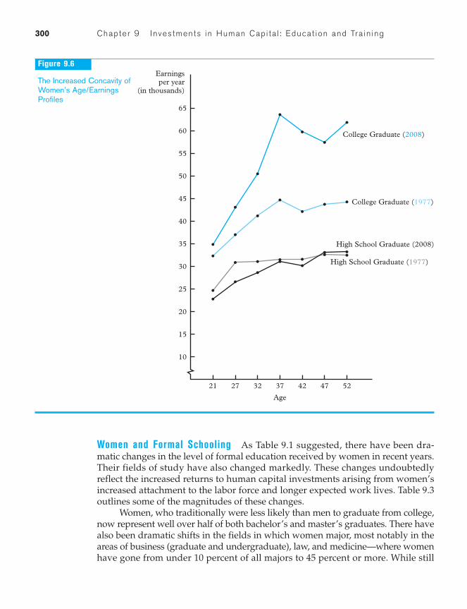
While human capital theory predicts that the traditional role of women inchild-rearing will lead to reduced incentives for training investments, it also sug-gests that as this role changes, the incentives for women to acquire training willchange. We should thus expect to observe a growing concavity in women’sage/earnings profiles over the past decades, and Figure 9.6 indicates that thisexpectation is generally supported.
The darker lines in Figure 9.6 are the 2008 profiles for college and highschool graduates that appeared in Figure 9.4. The lighter lines indicate the com-parable profiles for 1977 (adjusted to 2008 dollars using the Consumer Price Index[CPI]). A visual comparison reveals that the earnings profiles for both high schooland college graduates have become steeper for women in their twenties and thir-ties, especially among the college educated. This faster earnings growth amongwomen at the early stages of their careers suggests that they may be receivingmore on-the-job training than they did two decades ago.
18H. Frazis, M. Gittleman, M. Horrigan, and M. Joyce, “Results from the 1995 Survey of Employer-Provided Training,” Monthly Labor Review 121 (June 1998): 3–13.19For an article on women’s pay expectations and resulting outcomes, see Peter F. Orazem, James D.Werbel, and James C. McElroy, “Market Expectations, Job Search, and Gender Differences in StartingPay,” Journal of Labor Research 24 (Spring 2003): 307–321.
300 Chapter 9 Investments in Human Capi ta l : Educat ion and Tra in ing
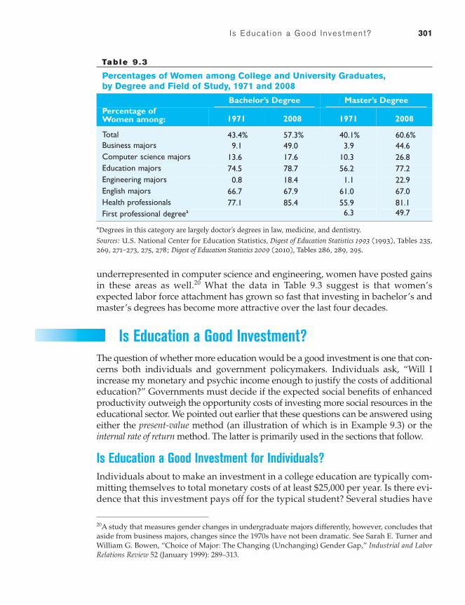
Women and Formal Schooling As Table 9.1 suggested, there have been dra-matic changes in the level of formal education received by women in recent years.Their fields of study have also changed markedly. These changes undoubtedlyreflect the increased returns to human capital investments arising from women’sincreased attachment to the labor force and longer expected work lives. Table 9.3outlines some of the magnitudes of these changes.
Women, who traditionally were less likely than men to graduate from college,now represent well over half of both bachelor’s and master’s graduates. There havealso been dramatic shifts in the fields in which women major, most notably in theareas of business (graduate and undergraduate), law, and medicine—where womenhave gone from under 10 percent of all majors to 45 percent or more. While still
10
15
20
25
30
35
40
45
50
55
60
65
Earningsper year
(in thousands)
College Graduate (1977)
High School Graduate (1977)
21 27 32 37 42 47 52
Age
College Graduate (2008)
High School Graduate (2008)
Figure 9.6
The Increased Concavity ofWomen’s Age/EarningsProfiles
Is Educat ion a Good Investment? 301
underrepresented in computer science and engineering, women have posted gainsin these areas as well.20 What the data in Table 9.3 suggest is that women’sexpected labor force attachment has grown so fast that investing in bachelor’s andmaster’s degrees has become more attractive over the last four decades.
Is Education a Good Investment?The question of whether more education would be a good investment is one that con-cerns both individuals and government policymakers. Individuals ask, “Will Iincrease my monetary and psychic income enough to justify the costs of additionaleducation?” Governments must decide if the expected social benefits of enhancedproductivity outweigh the opportunity costs of investing more social resources in theeducational sector. We pointed out earlier that these questions can be answered usingeither the present-value method (an illustration of which is in Example 9.3) or theinternal rate of return method. The latter is primarily used in the sections that follow.
Is Education a Good Investment for Individuals?Individuals about to make an investment in a college education are typically com-mitting themselves to total monetary costs of at least $25,000 per year. Is there evi-dence that this investment pays off for the typical student? Several studies have
20A study that measures gender changes in undergraduate majors differently, however, concludes thataside from business majors, changes since the 1970s have not been dramatic. See Sarah E. Turner andWilliam G. Bowen, “Choice of Major: The Changing (Unchanging) Gender Gap,” Industrial and LaborRelations Review 52 (January 1999): 289–313.
Tab le 9 .3
Percentages of Women among College and University Graduates, by Degree and Field of Study, 1971 and 2008
Bachelor’s Degree Master’s DegreePercentage of Women among: 1971 2008 1971 2008
Total 43.4% 57.3% 40.1% 60.6%Business majors 9.1 49.0 3.9 44.6Computer science majors 13.6 17.6 10.3 26.8Education majors 74.5 78.7 56.2 77.2Engineering majors 0.8 18.4 1.1 22.9English majors 66.7 67.9 61.0 67.0Health professionals 77.1 85.4 55.9 81.1First professional degreea 6.3 49.7
aDegrees in this category are largely doctor’s degrees in law, medicine, and dentistry.Sources: U.S. National Center for Education Statistics, Digest of Education Statistics 1993 (1993), Tables 235,269, 271–273, 275, 278; Digest of Education Statistics 2009 (2010), Tables 286, 289, 295.
302 Chapter 9 Investments in Human Capi ta l : Educat ion and Tra in ing
tried to answer this question by calculating the internal rates of return to educa-tional investments. While the methods and data used vary, these studies normallyestimate benefits by calculating earnings differentials at each age from age/earningsprofiles such as those in Figures 9.3 and 9.4. (Earnings are usually used to measurebenefits because higher wages and more stable jobs are both payoffs to more education.) All such studies have analyzed only the monetary, not the psychic,costs of and returns on educational investments.
Estimating the returns to an educational investment involves comparing theearnings of similar people who have different levels of education. Estimates usingconventional data sets statistically analyze the earnings increases associated withincreases in schooling, after controlling for the effects on earnings of other factorsthat can be measured, such as age, race, gender, health status, union status, and
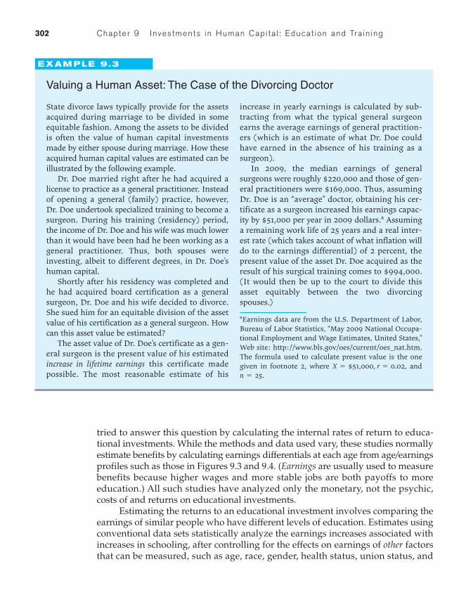
EXAM PLE 9.3
Valuing a Human Asset: The Case of the Divorcing Doctor
State divorce laws typically provide for the assetsacquired during marriage to be divided in someequitable fashion. Among the assets to be dividedis often the value of human capital investmentsmade by either spouse during marriage. How theseacquired human capital values are estimated can beillustrated by the following example.
Dr. Doe married right after he had acquired alicense to practice as a general practitioner. Insteadof opening a general (family) practice, however, Dr. Doe undertook specialized training to become asurgeon. During his training (residency) period,the income of Dr. Doe and his wife was much lowerthan it would have been had he been working as ageneral practitioner. Thus, both spouses wereinvesting, albeit to different degrees, in Dr. Doe’shuman capital.
Shortly after his residency was completed andhe had acquired board certification as a generalsurgeon, Dr. Doe and his wife decided to divorce.She sued him for an equitable division of the assetvalue of his certification as a general surgeon. Howcan this asset value be estimated?
The asset value of Dr. Doe’s certificate as a gen-eral surgeon is the present value of his estimatedincrease in lifetime earnings this certificate madepossible. The most reasonable estimate of his
increase in yearly earnings is calculated by sub-tracting from what the typical general surgeonearns the average earnings of general practition-ers (which is an estimate of what Dr. Doe couldhave earned in the absence of his training as asurgeon).
In 2009, the median earnings of generalsurgeons were roughly $220,000 and those of gen-eral practitioners were $169,000. Thus, assumingDr. Doe is an “average” doctor, obtaining his cer-tificate as a surgeon increased his earnings capac-ity by $51,000 per year in 2009 dollars.a Assuminga remaining work life of 25 years and a real inter-est rate (which takes account of what inflation willdo to the earnings differential) of 2 percent, thepresent value of the asset Dr. Doe acquired as theresult of his surgical training comes to $994,000.(It would then be up to the court to divide thisasset equitably between the two divorcingspouses.)
aEarnings data are from the U.S. Department of Labor,Bureau of Labor Statistics, “May 2009 National Occupa-tional Employment and Wage Estimates, United States,”Web site: http://www.bls.gov/oes/current/oes_nat.htm.The formula used to calculate present value is the onegiven in footnote 2, where andn = 25.
X = $51,000, r = 0.02,
Is Educat ion a Good Investment? 303
residential location. These studies, of which there have been hundreds, typicallyestimate rates of return that fall into the range of 5–12 percent.21 Interestingly,these rates of return are close to those typically found for other types of invest-ments, which—as explained later in Example 9.4—is what economic theorywould lead us to expect.
Ability Bias One problem with these conventional estimates is that they mayoverstate the gain an individual could obtain by investing in education, becausethey do not distinguish between the contribution that ability makes to higherearnings and the contribution made by schooling.22 The problem is that (a) peoplewho are smarter, harder working, and more dynamic are likely to obtain moreschooling, and (b) such people might be more productive, and hence earn higher-than-average wages, even if they did not complete more years of schooling thanothers. When measures of true ability are not observed or accounted for, the stud-ies attribute all the earnings differentials associated with college to college itselfand none to ability, even though some of the added earnings college graduatestypically receive may have been received by an equally able high school graduatewho did not attend college.
Some studies have attempted to control for ability by using measures ofintelligence quotient (IQ) or scores on aptitude tests, but there are continuing dis-putes over how much these tests reveal about innate abilities. One clever way tocontrol for ability without relying on these tests is to analyze earnings differencesamong sets of identical twins (see the Empirical Study at the end of this chapter).Identical twins have the same genes, so they will have the same innate abilities,and one would think that measuring earnings differences that are associated withdifferences in schooling within pairs of twins would yield an unbiased estimate ofthe returns to education. The most recent studies of twins estimate rates of returnthat are not too different from the conventional estimates noted earlier; thesestudies, then, suggest that ability bias in the conventional estimates may not bevery large.23 However, we must still worry about why two identical twins differin their educational levels!
21See David Card, “Estimating the Return to Schooling: Progress on Some Persistent EconometricProblems,” Econometrica 69 (September 2001): 1127–1160; and David Card, “The Causal Effect of Edu-cation on Earnings,” in Handbook of Labor Economics, eds. Orley Ashenfelter and David Card (NewYork: Elsevier, 1999), 1802–1863, for comprehensive reviews.22An investment in education should also raise wages more than overall wealth—which (recallingchapters 6 and 7) should cause hours of work to rise. Thus, some of the increased earnings from moreeducation could be associated with reduced leisure, which would constitute another source of upwardbias. This point is made by C. M. Lindsay, “Measuring Human Capital Returns,” Journal of PoliticalEconomy 79 (November/December 1971): 1195–1215.23See Orley Ashenfelter and Cecilia Rouse, “Income, Schooling, and Ability: Evidence from a NewSample of Identical Twins,” Quarterly Journal of Economics 113 (February 1998): 253–284; and AndrewLeigh and Chris Ryan, “Estimating Returns to Education Using Different Natural Experiment Tech-niques,” Economics of Education Review 27 (April 2008): 149–160.

304 Chapter 9 Investments in Human Capi ta l : Educat ion and Tra in ing
Selection Bias Innate ability is only one factor affecting human capital deci-sions that we have difficulty measuring. The psychic costs of schooling and indi-vidual discount rates are other variables that affect decisions about educationalinvestments, yet they cannot be measured. Why do these factors pose a problemfor estimating the rates of return to educational investments?
Suppose that Fred and George are twins, but for some reason, they differ intheir personal discount rates. Fred, with a relatively high discount rate of 12 per-cent, will not make an educational investment unless he estimates it will havereturns greater than 12 percent, while George has a lower discount rate and willmake investments as long as they are expected to bring him at least 8 percent.Because we must estimate rates of return from a sample that includes people withdifferent educational levels, we will have both “Freds” and “Georges” in our sam-ple. If those like Fred have chosen to stop their educational investments when thereturns were 12 percent, and those like George stopped theirs when returns were8 percent, the average rate of return estimated from our sample will fall some-where between 8 percent and 12 percent. While estimating this average rate ofreturn may be interesting, we are not estimating the rate of return for either Fredor George!
Estimating the rate of return for groups that are exactly similar in ability,psychic costs of education, and personal discount rates is difficult, because theorypredicts that those who are exactly alike will make the same decisions about humancapital investments—yet, we need differences in schooling to estimate its returns.Economists have tried, therefore, to find contexts in which people who are alikehave different levels of education because of factors beyond their control; theimplementation of compulsory schooling laws (laws that require children toremain in school until they reach a certain age) have provided one such context.Studies of high school dropouts—some of whom, by the accident of their birth-day, will have been forced into more schooling than others—have yielded esti-mated rates of return that lie slightly above the range of conventional estimates.24
These higher estimates are not too surprising, given that those in the studies(dropouts) probably have personal discount rates that are relatively high.
Is Education a Good Social Investment?The issue of education as a social investment has been of heightened interest inthe United States in recent years, especially because of three related develop-ments. First, product markets have become more global, increasing the elasticityof both product and labor demand. As a result, American workers are now facingmore competition from workers in other countries. Second, the growing availabil-ity of high-technology capital has created new products and production systems
24For a study that summarizes the issues and refers to similar studies, see Philip Oreopoulos, “Esti-mating Average and Local Average Treatment Effects of Education When Compulsory Schooling LawsReally Matter,” American Economic Review 96 (March 2006): 152–175.
Is Educat ion a Good Investment? 305
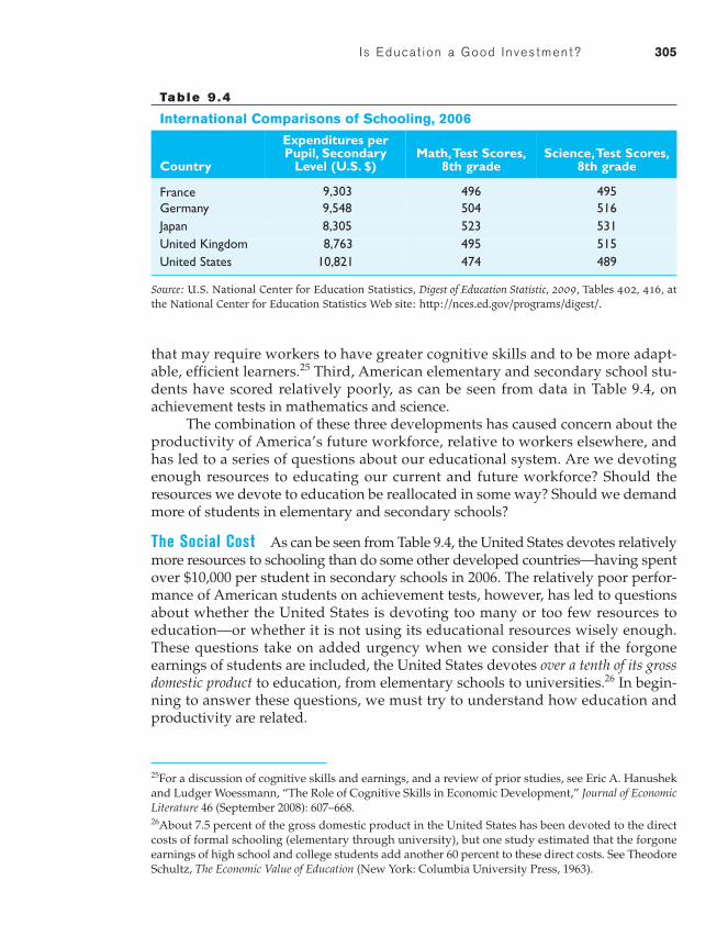
that may require workers to have greater cognitive skills and to be more adapt-able, efficient learners.25 Third, American elementary and secondary school stu-dents have scored relatively poorly, as can be seen from data in Table 9.4, onachievement tests in mathematics and science.
The combination of these three developments has caused concern about theproductivity of America’s future workforce, relative to workers elsewhere, andhas led to a series of questions about our educational system. Are we devotingenough resources to educating our current and future workforce? Should theresources we devote to education be reallocated in some way? Should we demandmore of students in elementary and secondary schools?
The Social Cost As can be seen from Table 9.4, the United States devotes relativelymore resources to schooling than do some other developed countries—having spentover $10,000 per student in secondary schools in 2006. The relatively poor perfor-mance of American students on achievement tests, however, has led to questionsabout whether the United States is devoting too many or too few resources toeducation—or whether it is not using its educational resources wisely enough.These questions take on added urgency when we consider that if the forgoneearnings of students are included, the United States devotes over a tenth of its grossdomestic product to education, from elementary schools to universities.26 In begin-ning to answer these questions, we must try to understand how education andproductivity are related.
25For a discussion of cognitive skills and earnings, and a review of prior studies, see Eric A. Hanushekand Ludger Woessmann, “The Role of Cognitive Skills in Economic Development,” Journal of EconomicLiterature 46 (September 2008): 607–668.26About 7.5 percent of the gross domestic product in the United States has been devoted to the directcosts of formal schooling (elementary through university), but one study estimated that the forgoneearnings of high school and college students add another 60 percent to these direct costs. See TheodoreSchultz, The Economic Value of Education (New York: Columbia University Press, 1963).
Tab le 9 .4
International Comparisons of Schooling, 2006
Country
Expenditures perPupil, Secondary
Level (U.S. $)Math,Test Scores,
8th gradeScience,Test Scores,
8th grade
France 9,303 496 495Germany 9,548 504 516Japan 8,305 523 531United Kingdom 8,763 495 515United States 10,821 474 489
Source: U.S. National Center for Education Statistics, Digest of Education Statistic, 2009, Tables 402, 416, atthe National Center for Education Statistics Web site: http://nces.ed.gov/programs/digest/.
306 Chapter 9 Investments in Human Capi ta l : Educat ion and Tra in ing
The Social Benefit The view that increased educational investments increaseworker productivity is a natural outgrowth of the observation that such invest-ments enhance the earnings of individuals who undertake them. If IndividualA’s productivity is increased because of more schooling, then society’s stock ofhuman capital has increased as a result. Some argue, however, that the addi-tional education received by Individual A also creates benefits for Individual B,who must work with A. If more schooling causes A to communicate moreclearly or solve problems more creatively, then B’s productivity will alsoincrease. In terms of concepts we introduced in chapter 1, education may createpositive externalities, so that the social benefits are larger than the privatebenefits.27
Others argue that the returns to society are smaller than the returns toindividuals. They believe that the educational system is used by society as ascreening device that sorts people by their (predetermined) ability. As dis-cussed later, this alternative view, in its extreme form, sees the educational sys-tem as a means of finding out who is productive, not of enhancing workerproductivity.
The Signaling Model An employer seeking to hire workers is nevercompletely sure of the actual productivity of any applicant, and in many cases,the employer may remain unsure long after an employee is hired. What anemployer can observe are certain indicators that firms believe to be correlatedwith productivity: age, experience, education, and other personal characteris-tics. Some indicators, such as age, are immutable. Others, such as formal educa-tion, can be acquired by workers. Indicators that can be acquired by individualscan be called signals; our analysis here will focus on the signaling aspect offormal education.
Let us suppose that firms wanting to hire new employees for particular jobsknow that there are two groups of applicants that exist in roughly equal propor-tions. One group has a productivity of 2, let us say, and the other has a productiv-ity of 1. Furthermore, suppose that these productivity levels cannot be changedby education and that employers cannot readily distinguish which applicants arefrom which group. If they were unable to make such distinctions, firms would beforced to assume that all applicants are “average”; that is, they would have toassume that each had a productivity of 1.5 (and would offer them wages of upto 1.5).
While workers in this simple example would be receiving what they wereworth on average, any firm that could devise a way to distinguish between the two
27For an example of a study (with references to others) on the external effects of education, see EnricoMoretti, “Workers’ Education, Spillovers, and Productivity: Evidence from Plant-Level Data,”American Economic Review 94 (June 2004): 656–690; and Susana Iranzo and Giovanni Peri, “SchoolingExternalities, Technology and Productivity: Theory and Evidence from U.S. States,” National Bureauof Economic Research, Working Paper No. 12440 (August 2006).
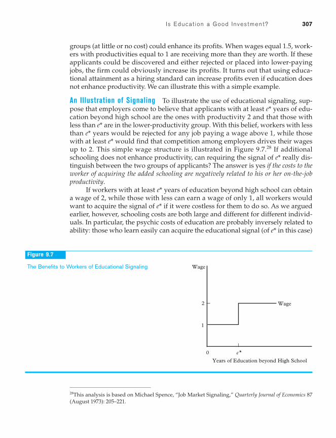
Is Educat ion a Good Investment? 307
groups (at little or no cost) could enhance its profits. When wages equal 1.5, work-ers with productivities equal to 1 are receiving more than they are worth. If theseapplicants could be discovered and either rejected or placed into lower-payingjobs, the firm could obviously increase its profits. It turns out that using educa-tional attainment as a hiring standard can increase profits even if education doesnot enhance productivity. We can illustrate this with a simple example.
An Illustration of Signaling To illustrate the use of educational signaling, sup-pose that employers come to believe that applicants with at least e* years of edu-cation beyond high school are the ones with productivity 2 and that those withless than are in the lower-productivity group. With this belief, workers with lessthan years would be rejected for any job paying a wage above 1, while thosewith at least would find that competition among employers drives their wagesup to 2. This simple wage structure is illustrated in Figure 9.7.28 If additionalschooling does not enhance productivity, can requiring the signal of really dis-tinguish between the two groups of applicants? The answer is yes if the costs to theworker of acquiring the added schooling are negatively related to his or her on-the-jobproductivity.
If workers with at least years of education beyond high school can obtaina wage of 2, while those with less can earn a wage of only 1, all workers wouldwant to acquire the signal of if it were costless for them to do so. As we arguedearlier, however, schooling costs are both large and different for different individ-uals. In particular, the psychic costs of education are probably inversely related toability: those who learn easily can acquire the educational signal (of in this case)e*
e*
e*
e*
e*e*
e*
0
Wage
Years of Education beyond High School
e*
2
1
Wage
Figure 9.7
The Benefits to Workers of Educational Signaling
28This analysis is based on Michael Spence, “Job Market Signaling,” Quarterly Journal of Economics 87(August 1973): 205–221.
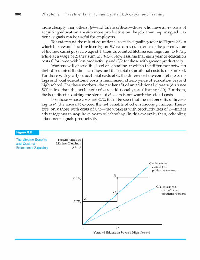
308 Chapter 9 Investments in Human Capi ta l : Educat ion and Tra in ing
more cheaply than others. If—and this is critical—those who have lower costs ofacquiring education are also more productive on the job, then requiring educa-tional signals can be useful for employers.
To understand the role of educational costs in signaling, refer to Figure 9.8, inwhich the reward structure from Figure 9.7 is expressed in terms of the present valueof lifetime earnings (at a wage of 1, their discounted lifetime earnings sum to while at a wage of 2, they sum to ). Now assume that each year of educationcosts C for those with less productivity and for those with greater productivity.
Workers will choose the level of schooling at which the difference betweentheir discounted lifetime earnings and their total educational costs is maximized.For those with yearly educational costs of C, the difference between lifetime earn-ings and total educational costs is maximized at zero years of education beyondhigh school. For these workers, the net benefit of an additional years (distanceBD) is less than the net benefit of zero additional years (distance A0). For them,the benefits of acquiring the signal of years is not worth the added costs.
For those whose costs are it can be seen that the net benefits of invest-ing in (distance BF) exceed the net benefits of other schooling choices. There-fore, only those with costs of —the workers with productivities of 2—find itadvantageous to acquire years of schooling. In this example, then, schoolingattainment signals productivity.
e*C>2
e*C>2,
e*
e*
C>2PVE2
PVE1,
0
Present Value ofLifetime Earnings
(PVE)
Years of Education beyond High School
C
PVE2
PVE1
e*
D
A
B
F
C/2(educationalcosts of moreproductive workers)
(educationalcosts of lessproductive workers)
Figure 9.8
The Lifetime Benefitsand Costs ofEducational Signaling
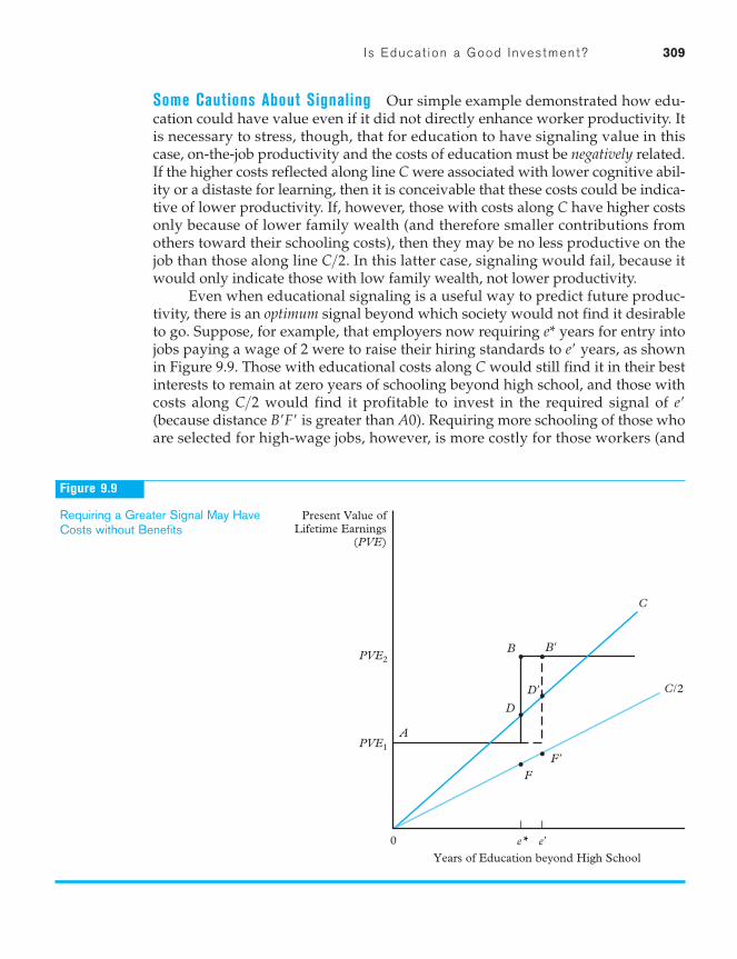
Is Educat ion a Good Investment? 309
Some Cautions About Signaling Our simple example demonstrated how edu-cation could have value even if it did not directly enhance worker productivity. Itis necessary to stress, though, that for education to have signaling value in thiscase, on-the-job productivity and the costs of education must be negatively related.If the higher costs reflected along line C were associated with lower cognitive abil-ity or a distaste for learning, then it is conceivable that these costs could be indica-tive of lower productivity. If, however, those with costs along C have higher costsonly because of lower family wealth (and therefore smaller contributions fromothers toward their schooling costs), then they may be no less productive on thejob than those along line . In this latter case, signaling would fail, because itwould only indicate those with low family wealth, not lower productivity.
Even when educational signaling is a useful way to predict future produc-tivity, there is an optimum signal beyond which society would not find it desirableto go. Suppose, for example, that employers now requiring years for entry intojobs paying a wage of 2 were to raise their hiring standards to years, as shownin Figure 9.9. Those with educational costs along C would still find it in their bestinterests to remain at zero years of schooling beyond high school, and those withcosts along would find it profitable to invest in the required signal of (because distance is greater than ). Requiring more schooling of those whoare selected for high-wage jobs, however, is more costly for those workers (and
A0B¿F¿e¿C>2
e¿e*
C>2
0
Present Value ofLifetime Earnings
(PVE)
Years of Education beyond High School
C
PVE2
PVE1
e* e�
D
D�
F�
A
B B�
F
C/2
Figure 9.9
Requiring a Greater Signal May HaveCosts without Benefits
310 Chapter 9 Investments in Human Capi ta l : Educat ion and Tra in ing
thus for society as a whole). While the new required signal would distinguishbetween the two groups of workers, it would do so at increased (and unneces-sary) costs to individuals, which cannot be socially optimal.
It clearly can be beneficial for individuals to invest in educational signals,but if schooling only has signaling value, is it a worthy investment for society tomake? If the only purpose of schools is to provide signals, why encourage invest-ments in the expansion or qualitative upgrading of schooling? If 50 years agobeing a high school graduate signaled above-average intelligence and work disci-pline, why incur the enormous costs of expanding college attendance only to findout that now these qualities are signaled by having a bachelor’s degree? The issueis of even more importance in less-developed countries, where mistakes in allo-cating extremely scarce capital resources could be disastrous (see Example 9.4).Before attempting to decide if schooling has social value when all it produces aresignals, let us first turn to the more basic question of whether we can figure out ifschooling enhances, or merely signals, human capital.
EXAM PLE 9.4
The Socially Optimal Level of Educational Investment
In addition to asking whether schooling is a goodsocial investment, we could also ask, “What is thesocially optimal level of schooling?” The generalprinciple guiding our answer to this question isthat society should increase or reduce its educa-tional investments until the marginal rate of return(to society) equals the marginal rate of return onother forms of capital investment (investment inphysical capital, for example).
The rationale for the above principle is that ifsociety has some funds it wants to invest, it willdesire to invest them in projects yielding the high-est rates of return. If an investment in physical cap-ital yields a 20 percent rate of return and the samefunds invested in schooling yield (all things consid-ered) only a 10 percent return, society will clearlyprefer to invest in physical capital. As long as thetwo rates of return differ, society could be madebetter off by reducing its investments in low-yieldprojects and increasing them in those with higherrates of return.
The text has discussed many of the difficultiesand biases inherent in estimating rates of return to
schooling. However, the general principle of equat-ing the rates of social return on all forms of invest-ments is still a useful one to consider. It suggests,for example, that capital-poor countries shouldinvest in additional schooling only if the returnsare very high—higher, in all probability, than therates of return required for optimality in more-capital-rich countries.
Indeed, the rates of return to both secondaryschooling and higher education appear to be gen-erally higher in less-developed countries than indeveloped countries. One review estimated that therate of return on secondary schooling investmentwas 10 percent for a developed country (on aver-age), while for a less-developed country, it was 13percent to 16 percent. Comparable rates of returnon investments in higher education were 9.5 per-cent and 11 percent, respectively.
Data from: George Psacharopoulos and Harry AnthonyPatrinos, “Returns to Investment in Education: A FurtherUpdate,” World Bank Policy Research, working paper no. 2881, September 2002, Table 3.
Is Educat ion a Good Investment? 311
Signaling or Human Capital? Direct evidence on the role schooling plays insociety is difficult to obtain. Advocates of the signaling viewpoint, for example,might point to the higher rates of return for college graduates than for collegedropouts as evidence that schooling is a signaling device.29 They argue thatwhat is learned in school is proportional to the time spent there and that anadded bonus (rate of return) just for a diploma is proof of the signaling hypoth-esis. Advocates of the view that schooling enhances human capital wouldcounter that those who graduate after four years have learned more than fourtimes what the freshman dropout has learned. They argue that dropouts aremore likely to be poorer students—the ones who overestimated their returns onschooling and quit when they discovered their mistake. Thus, their relativelylow rate of return is associated not with their dropping out but with their reasonfor dropping out.
To take another example, proponents of the human capital view could arguethat the fact that earnings differentials between college and high school graduatesgrow with age supports their view. If schooling were just a signaling device,employers would rely on it initially, but as they accumulated direct informationfrom experience with their employees, schooling would play a smaller role indetermining earnings. Signaling advocates could counter that continued growthin earnings differentials only illustrates that educational attainment was asuccessful signaling device.30
School Quality Given the difficulty of generating predictions of labor marketoutcomes that can directly distinguish the signaling from the human capitalhypothesis, you may wonder if there are other ways to resolve the debate.A research strategy with some potential grows out of issues related to schoolquality.
29Dropouts naturally have lower earnings than graduates, but because they have also invested less, itis not clear that their rates of return should be lower. For further discussion and evidence, see DavidA. Jaeger and Marianne E. Page, “Degrees Matter: New Evidence on Sheepskin Effects in the Returnsto Education,” Review of Economics and Statistics 78 (November 1996): 733–740. Thomas J. Kane andCecilia Elena Rouse, “Comment on W. Norton Grubb: ‘The Varied Economic Returns to Postsec-ondary Education: New Evidence from the Class of 1972,’” Journal of Human Resources 30 (Winter1995): 205–221, calls into question the benefits of graduation independent of the number of creditstaken.30Attempts to distinguish between the two views include Joseph Altonji, “The Effects of High SchoolCurriculum on Education and Labor Market Outcomes,” Journal of Human Resources 30 (Summer1995): 409–438; Andrew Weiss, “Human Capital vs. Signaling Explanations of Wages,” Journal of Eco-nomic Perspectives 9 (Fall 1995): 133–154; Wim Groot and Hessel Oosterbeek, “Earnings Effects of Dif-ferent Components of Schooling: Human Capital versus Screening,” Review of Economics and Statistics76 (May 1994): 317–321; Kelly Bedard, “Human Capital versus Signaling Models: University Accessand High School Dropouts,” Journal of Political Economy 109 (August 2001): 749–775; and Harley Frazis,“Human Capital, Signaling, and the Pattern of Returns to Education,” Oxford Economic Papers 54 (April2002): 298–320.
312 Chapter 9 Investments in Human Capi ta l : Educat ion and Tra in ing
As mentioned earlier, concerns have been raised about the cognitiveachievement of American students. If schooling primarily performs a signalingfunction, by helping to discover people’s cognitive abilities, we would not neces-sarily look to the educational system to remedy the problem of low cognitiveachievement. However, if schooling can enhance the kinds of skills that pay off inthe labor market, then increased investment in the quality of the nation’s schoolscould be warranted.
Proponents of the signaling and human capital views of education can agreethat people of higher cognitive ability are likely to be more productive; wherethey disagree is whether better schools can enhance worker productivity byimproving cognitive skills. Advocates of the signaling viewpoint cite a substan-tial literature suggesting it is difficult to demonstrate a relationship betweenschooling expenditures and student performance on tests of cognitive skill,although the evidence on this question is mixed.31 Advocates of the human capi-tal view, however, find support in studies of earnings and school quality. Thesestudies generally indicate that students attending higher-quality schools (that is,ones with greater resources per student) have higher subsequent earnings, otherthings equal.32
Clearly, assessments of the social returns to schooling that examine the role ofschool quality have so far yielded somewhat ambiguous results. Better schools mayenhance labor market earnings, but evidence that they enhance measured cogni-tive abilities is mixed. One possibility, of course, is that better schools enhance productivity by enhancing creative skills or better work habits—characteristics that may be valued in the labor market but not captured especially well by stan-dardized tests of cognitive achievement. Another possibility, however, is that better
31See, for example, Eric A. Hanushek, John F. Kain, Daniel M. O’Brien, and Steven G. Rivkin, “TheMarket for Teacher Quality,” National Bureau of Economic Research, Working Paper No. 11154 (Feb-ruary 2005); Charles T. Clotfelter, Helen F. Ladd, and Jacob L. Vigdor, “How and Why Do Teacher Cre-dentials Matter for Student Achievement?” National Bureau of Economic Research, Working PaperNo. 12828 (January 2007); Thomas J. Kane, Jonah E. Rockoff, and Douglas Staigner, “What Does Certi-fication Tell Us About Teacher Effectiveness? Evidence from New York City,” National Bureau of Eco-nomic Research, Working Paper No. 12155 (July 2006); Eric A. Hanushek and Dennis D. Kimko,“Schooling, Labor Force Quality, and the Growth of Nations,” American Economic Review 90 (December2000): 1184–1208; and Alan B. Krueger and Diane M. Whitmore, “The Effect of Attending a Small Classin the Early Grades on College-Test Taking and Middle School Test Results: Evidence from ProjectSTAR,” Economic Journal 111 (January 2001): 1–28.32For citations to the literature analyzing links between school resources and student outcomes, seeGeorge A. Akerlof and Rachel E. Kranton, “Identity and Schooling: Some Lessons for the Economicsof Education,” Journal of Economic Literature 40 (December 2002): 1167–1201. This article attempts toidentify sociological factors that might help resolve the disparate results obtained in economic analy-ses that relate schooling resources to educational results. For a more recent study, see Orley Ashenfel-ter, William J. Collins, and Albert Yoon, “Evaluating the Role of Brown vs. Board of Education in SchoolEqualization, Desegregation, and the Income of African Americans,” National Bureau of EconomicResearch, Working Paper No. 11394 (June 2005).
Is Educat ion a Good Investment? 313
schools give students better information about their own interests and abilities,thus helping them to make more successful career choices. Some important ques-tions, then, remain unanswered.
Does the Debate Matter? In the end, perhaps the debate between advocates ofthe signaling and human capital views of schooling is not terribly important. Thefact is that schooling investments offer individuals monetary rates of return thatare comparable to those received from other forms of investment. For individualsto recoup their human capital investment costs requires willingness on the part ofemployers to pay higher wages to people with more schooling; and for employ-ers to be willing to do this, schools must be providing a service that they couldnot perform more cheaply themselves.
For example, we argued earlier that to profit from an investment of $100,000in a college education, college graduates must be paid at least $3,652 more peryear than they would have received otherwise. Naturally, this requires that theyfind employers who are willing to pay them the higher yearly wage. If collegemerely helps reveal who is more productive, employers who believe they couldfind this out for less than a yearly cost of $3,652 per worker would clearly haveincentives to adopt their own methods of screening workers.
The fact that employers continue to emphasize (and pay for) educationalrequirements in the establishment of hiring standards suggests one of two things.Either more education does enhance worker productivity or it is a less expensivescreening tool than any other that firms could use. In either case, the fact thatemployers are willing to pay a high price for an educated workforce seems tosuggest that education produces social benefits.33
Is Public Sector Training a Good Social Investment?Policymakers should also ask whether government job training programs can bejustified based on their returns. During the past four decades, the federal govern-ment has funded a variety of these programs that primarily targeted disadvan-taged men, women, and youth. Some programs have served trainees who appliedvoluntarily, and others have been mandatory programs for public assistancerecipients (who stood to lose benefits if they did not enroll). Some of these pro-grams have provided relatively inexpensive help in searching for work, whileothers have directly provided work experience or (in the case of the Job Corps)comprehensive services associated with living away from home. Over thesedecades, however, roughly half of those enrolled received classroom trainingat vocational schools or community colleges, and another 15 percent received
33Kevin Lang, “Does the Human Capital/Educational Sorting Debate Matter for DevelopmentPolicy?” American Economic Review 84 (March 1994): 353–358, comes to a similar conclusion through amore formal argument.

314 Chapter 9 Investments in Human Capi ta l : Educat ion and Tra in ing
E M P I R I C A L S T U D Y
Estimating the Returns to Education Using a Sampleof Twins: Coping with the Problem of UnobservedDifferences in Ability
Researchers doing empirical studiesmust always be aware of how their
results are affected by the problem ofomitted variables. It is rare that we haveaccess to data on all relevant indepen-dent variables, and the regression tech-niques described in Appendix 1A containan error term that explicitly assumes thevariables we have do not fully explain allthe variation in a given dependent vari-able. If an omitted variable is not corre-lated with any observed independentvariable, there is no bias imparted to theestimates of how the independent vari-ables affect the dependent variable.
However, if an omitted indepen-dent variable is correlated with a partic-ular observed one, the estimated effectof the observed variable will be biased.The omitted variables bias, and one solu-tion to it, can be illustrated by the prob-lem of estimating the returns to schoolingwhen researchers do not have data oninnate learning ability (which is very difficult to observe).
The returns to education are con-ventionally estimated by using multi-variate regression techniques to analyze,for a cross-section of workers, how muchearnings are increased by an additionalyear of schooling—after controlling forother observed factors that influenceearnings. However, if people with higherinnate capacities for learning (higherability) are the very ones who pursue
more education, then estimates of thereturns to schooling will also includeany labor market rewards for abilityunless researchers are able to measureinnate learning ability. Put differently, ifeducation and ability levels are posi-tively correlated, but we do not observedata on innate ability, our estimates ofthe effects of schooling will be biasedupward (we discussed this earlier asability bias). Lacking a way to control forlearning ability, then, makes it problem-atic to estimate how much more a typicalperson (with a given ability level) wouldearn if he or she invested in another yearof schooling. Can we find a way to cor-rect for ability bias, and if so, can we esti-mate how large that bias is?
A clever way to avoid the problemsof ability bias is to use a sample of identi-cal twins, because such twins have pre-cisely the same genetic material and thusthe same native abilities. With the sameability and family background, identicaltwins should have the same incentives foreducational investments; however, ran-dom factors (marriage, divorce, careerinterests) can intervene and cause twins tohave different schooling levels. By statisti-cally analyzing, for several sets of twins,how the earnings differences betweeneach twin in a pair are affected by differ-ences in their years of schooling, we canestimate the returns to schooling in a waythat is free of ability bias.
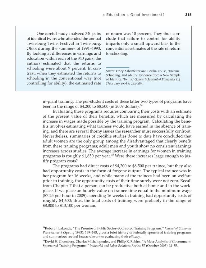
Is Educat ion a Good Investment? 315
in-plant training. The per-student costs of these latter two types of programs havebeen in the range of $4,200 to $8,500 (in 2009 dollars).34
Evaluating these programs requires comparing their costs with an estimateof the present value of their benefits, which are measured by calculating theincrease in wages made possible by the training program. Calculating the bene-fits involves estimating what trainees would have earned in the absence of train-ing, and there are several thorny issues the researcher must successfully confront.Nevertheless, summaries of credible studies done to date have concluded thatadult women are the only group among the disadvantaged that clearly benefitfrom these training programs; adult men and youth show no consistent earningsincreases across studies. The average increase in earnings for women in trainingprograms is roughly $1,850 per year.35 Were these increases large enough to jus-tify program costs?
The programs had direct costs of $4,200 to $8,500 per trainee, but they alsohad opportunity costs in the form of forgone output. The typical trainee was inher program for 16 weeks, and while many of the trainees had been on welfareprior to training, the opportunity costs of their time surely were not zero. Recallfrom Chapter 7 that a person can be productive both at home and in the work-place. If we place an hourly value on trainee time equal to the minimum wage($7.25 per hour in 2009), spending 16 weeks in training had opportunity costs ofroughly $4,600; thus, the total costs of training were probably in the range of$8,800 to $13,100 per woman.
34Robert J. LaLonde, “The Promise of Public Sector–Sponsored Training Programs,” Journal of EconomicPerspectives 9 (Spring 1995): 149–168, gives a brief history of federally sponsored training programsand summarizes several issues relevant to evaluating their efficacy.35David H. Greenberg, Charles Michalopoulos, and Philip K. Robins, “A Meta-Analysis of Government-Sponsored Training Programs,” Industrial and Labor Relations Review 57 (October 2003): 31–53.
One careful study analyzed 340 pairsof identical twins who attended the annualTwinsburg Twins Festival in Twinsburg,Ohio, during the summers of 1991–1993.By looking at differences in earnings andeducation within each of the 340 pairs, theauthors estimated that the returns toschooling were about 9 percent. In con-trast, when they estimated the returns toschooling in the conventional way (notcontrolling for ability), the estimated rate
of return was 10 percent. They thus con-clude that failure to control for abilityimparts only a small upward bias to theconventional estimates of the rate of returnto schooling.
Source: Orley Ashenfelter and Cecilia Rouse, “Income,Schooling, and Ability: Evidence from a New Sampleof Identical Twins,” Quarterly Journal of Economics 113(February 1998): 253–284.
316 Chapter 9 Investments in Human Capi ta l : Educat ion and Tra in ing
If benefits of $1,850 per year were received annually for 20 years after train-ing, and if the appropriate discount rate is 2 percent, the present value of benefitscomes to roughly $30,250. Benefits of this magnitude are clearly in excess of costs.Indeed, the present value of benefits for voluntary training would still be inexcess of $11,000 (the approximate midpoint of the cost range) if the yearly earn-ings increases lasted for just 7 years.36
36Paul Lengermann, “How Long Do the Benefits of Training Last? Evidence of Long Term EffectsAcross Current and Previous Employers,” Research in Labor Economics 18 (1999): 439–461, found thatthe gains from formal and company training last at least nine years. For an analysis of the returnsto Job Corps training, see Peter Z. Schochet, John Burghardt, and Sheena McConnell, “Does JobCorps Work? Impact Findings from the National Job Corps Study,” American Economic Review 98(December 2008): 1864–1886. For reference to studies of vocational education, see Paul Ryan, “TheSchool-to-Work Transition: A Cross-National Perspective,” Journal of Economic Literature 29 (March2001): 34–92.
Review Questions1. Women receive lower wages, on average,
than men of equal age. What concepts ofhuman capital help to explain this phe-nomenon? Explain. Why does the dis-crepancy between earnings for men andwomen grow with age?
2. “The vigorous pursuit by a society oftax policies that tend to equalize wagesacross skill groups will frustrate thegoal of optimum resource allocation.”Comment.
3. A few years ago, a prominent medical col-lege inadvertently accepted more appli-cants than it could accommodate in itsfirst-year class. Not wanting to arbitrarilydelay the entrance date of the studentsadmitted, it offered them one year of freetuition if they would delay their medicalstudies by one year. Discuss the factorsentering into a student’s assessment ofwhether he or she should take this offer.
4. When Plant X closed, Employer Y (whichoffers no training to its workers) hiredmany of X’s employees after they had com-pleted a lengthy, full-time retraining pro-gram offered by a local agency. The city’sEqual Opportunity Commission noticed
that the workers Employer Y hired from Xwere predominantly young, and itlaunched an age-discrimination investiga-tion. During this investigation, Employer Yclaimed that it hired all the applicants fromX who had successfully completed theretraining program, without regard to age.From what you know of human capital the-ory, does Y’s claim sound credible? Explain.
5. Why do those who argue that more educa-tion “signals” greater ability believe thatthe most able people will obtain the mosteducation?
6. A study shows that for American highschool dropouts, obtaining a GeneralEquivalency Degree (GED) by part-timestudy after high school has very little pay-off. It also shows, however, that for immi-grants who did not complete high schoolin their native countries, obtaining a GEDhas a relatively large payoff. Can signalingtheory be used to explain these results?
7. In many countries, higher education isheavily subsidized by the government(that is, university students do not bear thefull cost of their college education). Whilethere may be good reasons for heavily
Problems 317
Problems1. Becky works in sales but is considering
quitting work for two years to earn anMBA. Her current job pays $40,000 peryear (after taxes), but she could earn$55,000 per year (after taxes) if she had amaster’s degree in business administra-tion. Tuition is $10,000 per year, and thecost of an apartment near campus is equalto the $10,000 per year she is currentlypaying. Becky’s discount rate is 6 percentper year. She just turned 48 and plans toretire when she turns 60, whether or notshe gets her MBA. Based on this informa-tion, should she go to school to earn herMBA? Explain carefully.
2. (Appendix). Suppose that the supply curvefor optometrists is given by while the demand curve is given by
where annual earnings inthousands of dollars per year and
of optometrists.a. Find the equilibrium wage and
employment levels.b. Now, suppose that the demand for
optometrists increases and the new
thousandsL =
W =50 - W,LD =
-6 + 0.6W,Ls =
demand curve is Assume that this market is subject tocobwebs because it takes about threeyears to produce people who specializein optometry. While this adjustment istaking place, the short-run supply ofoptometrists is fixed. Calculate thewage and employment levels in each ofthe first three rounds, and find the newlong-run equilibrium. Draw a graph toshow these events.
3. Suppose you are offered $100 now or $125in five years. Let the interest rate be 4 per-cent. Calculate the present value of the$125 option. Which option should youtake if your goal is to choose the optionwith the larger present value?
4. Prepaid college tuition plans, also knownas Prepaid Education Arrangements (PEAs),allow you to prepay college tuition at present-day prices. The value of the invest-ment is guaranteed by the state to coverpublic college tuition, regardless of itsfuture cost. You are considering the pur-chase of an education certificate for
L ¿D = 66 - W.
subsidizing university education, there arealso some dangers in it. Using human cap-ital theory, explain what these dangers are.
8. Many crimes against property (burglary,for example) can be thought of as acts thathave immediate gains but run the risk oflong-run costs. If imprisoned, the crimi-nal loses income from both criminal andnoncriminal activities. Using the frame-work for occupational choice in the longrun, analyze what kinds of people aremost likely to engage in criminal activi-ties. What can society do to reduce crime?
9. A recent study in Great Britain found thatwomen doctors are much more likelythan male doctors to be in the field of
all-purpose family medicine, choosingnot to pursue additional training in one ofthe specialties (surgery, for example). Italso found that half of the female doctorsin family medicine worked part-time,while only 10 percent of the males in fam-ily medicine did so. Use human capitaltheory to analyze whether these two factsare likely to be related. Explain fully.
10. The following statement was overheard ata party: “It is just not right that Joe, whonever went to college, makes more thanKen, who has a master’s degree. Peoplewith higher degrees deserve to earnmore!” Use human capital theory to com-ment on this quotation.

318 Chapter 9 Investments in Human Capi ta l : Educat ion and Tra in ing
$25,000, which will cover the future tuitioncosts of your 8-year-old daughter. Youexpect the tuition costs of your daughter’sbachelor’s degree to total $50,000 in 10years. What would your personal discountrate need to be in order for it to be worth-while for you to make the investment andpurchase the certificate?
5. Theodore is considering a 1-year trainingprogram, which charges $20,000 in tuition,to learn how to install airport-screening
equipment. If he enrolls in the program,his opportunity cost in forgone income isthe $100,000 per year he can now earn. Aftercompleting the program, he is promised ajob for 5 years, with a yearly salary of$130,000. (After 5 years, the equipment isexpected to be obsolete, but Theodoreplans to retire at that time anyway.)Assume Theodore’s personal discount rateis 5 percent. Should Theodore enroll in theprogram? Why? (Show your calculations.)
Selected ReadingsBecker, Gary. Human Capital. New York:
National Bureau of Economic Research,1975.
Borjas, George J. “Earnings Determination:A Survey of the Neoclassical Approach.” InThree Worlds of Labor Economics, eds. GarthMangum and Peter Philips. Armonk, N.Y.:M. E. Sharpe, 1988.
Card, David. “The Causal Effect of Educationon Earnings.” In Handbook of Labor Economics,eds. Orley Ashenfelter and David Card. NewYork: Elsevier, 1999.
Clotfelter, Charles T., Ronald G. Ehrenberg,Malcolm Getz, and John Siegfried. EconomicChallenges in Higher Education. Chicago: Uni-versity of Chicago Press, 1991.
Friendlander, Daniel, David H. Greenberg, andPhilip K. Robins. “Evaluating Government
Training Programs for the Economically Dis-advantaged.” Journal of Economic Literature35 (December 1997): 1809–1855.
Krueger, Alan B., and Mikael Lindahl. “Educa-tion for Growth: Why and for Whom?”Journal of Economic Literature 39 (December2001): 1101–1136.
Mincer, Jacob. Schooling, Experience, and Earn-ings. New York: National Bureau of Eco-nomic Research, 1974.
Schultz, Theodore. The Economic Value of Educa-tion. New York: Columbia University Press,1963.
Spence, Michael. “Job Market Signaling.”Quarterly Journal of Economics 87 (August1973): 355–374.
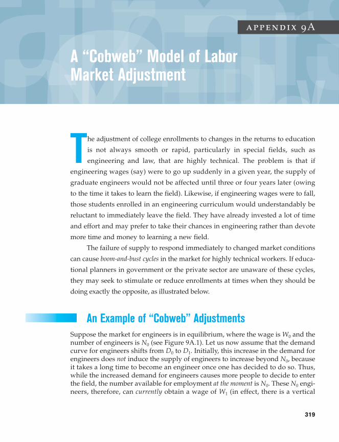
appendix 9A
A “Cobweb” Model of LaborMarket Adjustment
319
The adjustment of college enrollments to changes in the returns to education
is not always smooth or rapid, particularly in special fields, such as
engineering and law, that are highly technical. The problem is that if
engineering wages (say) were to go up suddenly in a given year, the supply of
graduate engineers would not be affected until three or four years later (owing
to the time it takes to learn the field). Likewise, if engineering wages were to fall,
those students enrolled in an engineering curriculum would understandably be
reluctant to immediately leave the field. They have already invested a lot of time
and effort and may prefer to take their chances in engineering rather than devote
more time and money to learning a new field.
The failure of supply to respond immediately to changed market conditions
can cause boom-and-bust cycles in the market for highly technical workers. If educa-
tional planners in government or the private sector are unaware of these cycles,
they may seek to stimulate or reduce enrollments at times when they should be
doing exactly the opposite, as illustrated below.
An Example of “Cobweb” AdjustmentsSuppose the market for engineers is in equilibrium, where the wage is and thenumber of engineers is (see Figure 9A.1). Let us now assume that the demandcurve for engineers shifts from to Initially, this increase in the demand forengineers does not induce the supply of engineers to increase beyond becauseit takes a long time to become an engineer once one has decided to do so. Thus,while the increased demand for engineers causes more people to decide to enterthe field, the number available for employment at the moment is These engi-neers, therefore, can currently obtain a wage of (in effect, there is a verticalW1
N0N0.
N0,D1.D0
N0
W0
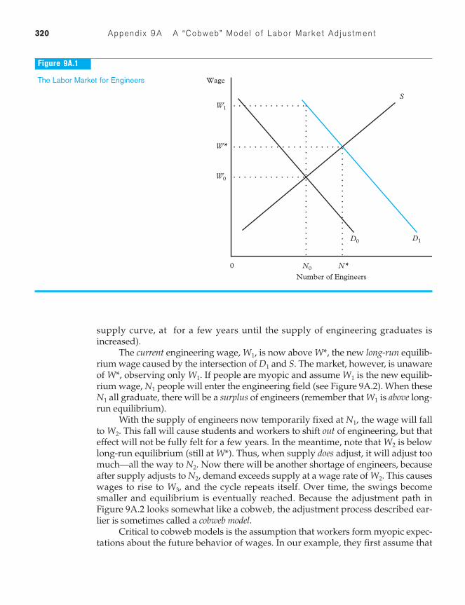
320 Appendix 9A A “Cobweb” Model of Labor Market Adjustment
supply curve, at for a few years until the supply of engineering graduates isincreased).
The current engineering wage, is now above the new long-run equilib-rium wage caused by the intersection of and S. The market, however, is unawareof observing only If people are myopic and assume is the new equilib-rium wage, people will enter the engineering field (see Figure 9A.2). When these
all graduate, there will be a surplus of engineers (remember that is above long-run equilibrium).
With the supply of engineers now temporarily fixed at the wage will fallto This fall will cause students and workers to shift out of engineering, but thateffect will not be fully felt for a few years. In the meantime, note that is belowlong-run equilibrium (still at ). Thus, when supply does adjust, it will adjust toomuch—all the way to Now there will be another shortage of engineers, becauseafter supply adjusts to demand exceeds supply at a wage rate of This causeswages to rise to and the cycle repeats itself. Over time, the swings becomesmaller and equilibrium is eventually reached. Because the adjustment path inFigure 9A.2 looks somewhat like a cobweb, the adjustment process described ear-lier is sometimes called a cobweb model.
Critical to cobweb models is the assumption that workers form myopic expec-tations about the future behavior of wages. In our example, they first assume that
W3,W2.N2,
N2.W*
W2
W2.N1,
W1N1
N1
W1W1.W*,D1
W*,W1,
0
Wage
Number of Engineers
S
W*
W1
N0
. . .
. . .
. . .
. . .
. . .
. . .
. .
. . .
. . .
. . .
. . . . . . . . . . . . . .
. . . . . . . . . . . . . . . . . . .
. . . . . . . . . . . . . .
D0 D1
W0
. . .
. . .
. . .
. . .
. . .
. . .
. . .
N*
Figure 9A.1
The Labor Market for Engineers
Rat ional Expectat ions 321
will prevail in the future and ignore the possibility that the occupational choicedecisions of others will, in four years, drive the wage below Just how workers(and other economic actors, such as investors and taxpayers) form expectationsabout future wage (price) levels is very important to the understanding of manykey issues affecting the labor market.1
Adaptive ExpectationsThe simplest and most naive way to predict future wage levels is to assume thatwhat is observed today is what will be observed in the future; this naive assump-tion, as noted earlier, underlies the cobweb model. A more sophisticated way toform predictions about the future is with an adaptive expectations approach. Adap-tive expectations are formed by setting future expected wages equal to a weightedaverage of current and past wages. While more weight may be given to currentthan past wages in forecasting future wage levels, changes in those levels prior tothe current period are not ignored; thus, it is likely that wage expectations formedadaptively do not alternatively overshoot and undershoot the equilibrium wageby as much as those formed using the naive approach. If, however, adaptive expec-tations also lead workers to first overpredict and then underpredict the equilib-rium wage, cobweb like behavior of wages and labor supply will still be observed(although the fluctuations will be of a smaller magnitude if the predictions arecloser to the mark than those made naively).
Rational ExpectationsThe most sophisticated way to predict future market outcomes is to use a full-blown model of the labor market. Those who believe in the rational expectationsmethod of forming predictions about future wages assume that workers do havesuch a model in their heads, at least implicitly. Thus, they will realize that amarked increase in the earnings of engineers (say) is likely to be temporary,because supply will expand and eventually bring the returns to an investment inengineering skills in line with those for other occupations. Put differently, therational expectations model assumes workers behave as if they have taken (andmastered!) a good course in labor economics and that they will not be fooled intooverpredicting or underpredicting future wage levels.
W1.W1
1Also critical to cobweb models is that the demand curve be flatter than the supply curve; if it is not, thecobweb explodes when demand shifts and an equilibrium wage is never reached. An exploding cobwebmodel is an example from economics of the phenomenon of chaos. For a general introduction to this fas-cinating topic, see James Gleick, Chaos (New York: Penguin Books, 1987). For an article on chaos theoryin the economic literature, see William J. Baumol and Jess Benhabib, “Chaos: Significance, Mechanism,and Economic Applications,” Journal of Economic Perspectives 3 (Winter 1989): 77–106.
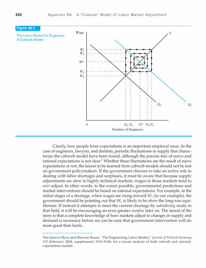
322 Appendix 9A A “Cobweb” Model of Labor Market Adjustment
0
Wage
Number of Engineers
S
W*
W1
N0. .
. . .
. . .
. . .
. . .
. . .
. .
. . . . . . . . . . . . . . . . . . .
. . . . . . . . . . . . . . . . .
. . . . . . . . . . . . . . . . . . .
D0 D1
W2
. . . . . . . . . . . . . . . . .
. . . . . . . . . . . . . . . . . . . . . . .
. . .
. . .
. . .
. . .
. . .
. . .
. . .
. . .
. . .
. . .
. . .
. . .
. . .
. .
. . .
. . .
. . .
. . .
. . .
. . .
. . .
. . .
.
. . .
. . .
. . .
. . .
. . .
. . .
. . .
W3
W0
N2 N* N1N3
Figure 9A.2
The Labor Market for Engineers:A Cobweb Model
Clearly, how people form expectations is an important empirical issue. In thecase of engineers, lawyers, and dentists, periodic fluctuations in supply that charac-terize the cobweb model have been found, although the precise mix of naive andrational expectations is not clear.2 Whether these fluctuations are the result of naiveexpectations or not, the lesson to be learned from cobweb models should not be loston government policymakers. If the government chooses to take an active role indealing with labor shortages and surpluses, it must be aware that because supplyadjustments are slow in highly technical markets, wages in those markets tend toover-adjust. In other words, to the extent possible, governmental predictions andmarket interventions should be based on rational expectations. For example, at theinitial stages of a shortage, when wages are rising toward (in our example), thegovernment should be pointing out that is likely to be above the long-run equi-librium. If instead it attempts to meet the current shortage by subsidizing study inthat field, it will be encouraging an even greater surplus later on. The moral of thestory is that a complete knowledge of how markets adjust to changes in supply anddemand is necessary before we can be sure that government intervention will domore good than harm.
W1
W1
2See Jaewoo Ryoo and Sherwin Rosen, “The Engineering Labor Market,” Journal of Political Economy112 (February 2004, supplement): S110–S140, for a recent analysis of both cobweb and rational-expectations models.