Investment Style Volatility and Mutual Fund Performance

Keith C. Brown Department of Finance, B6600 McCombs School of Business

University of Texas Austin, Texas 78712

(512) 471-6520 E-mail: keith.brown@mccombs.utexas.edu

W. V. Harlow

Putnam Investments One Post Office Square

Boston, Massachusetts 02109 (617) 760-7023

E-mail: van_harlow@putnam.com

Hanjiang Zhang Division of Banking and Finance

Nanyang Business School Nanyang Technological University

Nanyang Avenue Singapore 639798 (65) 6790-6118

E-mail: zhanghj@ntu.edu.sg ABSTRACT: We develop a holdings-based statistic to measure the volatility of a fund’s investment style characteristic profile over time. On average, funds with lower levels of style volatility significantly outperform more style-volatile funds on a risk-adjusted basis. We show that style volatility has a distinct impact on future fund performance compared to fund expenses or past risk-adjusted returns, with the level of indirect style volatility being the primary determinant of the overall effect. We conclude that deciding to maintain a less volatile investment style is an important aspect of the portfolio management process.

Current Draft: May 28, 2015

We are grateful for the comments of Andres Almazan, Nick Bollen, Mark Carhart, Dave Chapman, Wayne Ferson, Douglas Foster, William Goetzmann, Jennifer Huang, Bob Jones, Robert Litterman, Paula Tkac, Clemens Sialm, Laura Starks, Laurens Swinkels, Sheridan Titman, and Russ Wermers on earlier versions of this study. Earlier versions were also presented at the Financial Management Association European Conference, University of Texas Finance seminar, the Goldman Sachs Asset Management seminar, the Atlanta Federal Reserve Board Financial Markets Conference, and the Erasmus University Conference on Professional Asset Management. The opinions and analyses presented herein are those of the authors and do not necessarily represent the views of Putnam Investments.

Investment Style Volatility and Mutual Fund Performance

ABSTRACT

We develop a holdings-based statistic to measure the volatility of a fund’s investment style characteristic profile over time. On average, funds with lower levels of style volatility significantly outperform more style-volatile funds on a risk-adjusted basis. We show that style volatility has a distinct impact on future fund performance compared to fund expenses or past risk-adjusted returns, with the level of indirect style volatility being the primary determinant of the overall effect. We conclude that deciding to maintain a less volatile investment style is an important aspect of the portfolio management process.

JEL Classification: G11, G14 Key Words: style investing, style volatility, performance persistence

Investment Style Volatility and Mutual Fund Performance 1. Introduction

There is by now ample evidence that an equity mutual fund’s investment style has become

deeply ingrained in how the fund is defined and the returns it produces. Indeed, researchers and

portfolio managers alike have long been aware of the benefits of forming stock portfolios that

emphasize various firm-related attributes (such as price-earnings ratios, market capitalization, or

return momentum). For example, Capaul et al. (1993), Fama and French (1998), and Chan and

Lakonishok (2004) all show that portfolios of value stocks outperform portfolios of growth

stocks on a long-term, risk-adjusted basis and that this “value premium” is a pervasive feature of

global capital markets, despite some disagreements as to why this premium occurs.

Additionally, Malkiel (1995) demonstrates that a fund’s ability to outperform a benchmark such

as the S&P 500 is related to its objective class, which has led other researchers (e.g., Brown and

Goetzmann (1997)) to question the efficacy of traditional methods for classifying funds.

In this study, we consider an aspect of the investment style question that has received little

attention in the literature; namely, the impact on performance associated with the level of

investment style volatility in the portfolio. Specifically, we define style volatility as the degree to

which the portfolio’s investment style characteristics shift over time as a result of how the

manager chooses to implement the fund’s style mandate; a portfolio with less (more) style

volatility can be thought of as one with a more (less) predictable implementation of its style

strategy. We then pose the following question: Do investors benefit from managers who

maintain their designated investment strategy on a more volatile or on a less volatile basis? That

is, regardless of what the specific investment mandate happens to be, does a manager who keeps

a tighter control on the volatility of that style decision add value relative to a manager that allows

2

the portfolio’s style to drift more over time? The underlying premise of this investigation is that

level of volatility resulting from how a manager implements the fund’s investment mandate

should be related to the returns it produces.

What is not necessarily clear, however, is the probable direction of this relationship. On

one hand, there are several potential reasons why, ceteris paribus, portfolios with a lower level of

style volatility (i.e., more style predictability) should produce superior returns. First, it is likely

that less style-volatile funds exhibit less portfolio turnover and, hence, have lower transaction

costs than funds that allow their style to drift. Second, it is possible that managers who act

opportunistically will end up altering the risk of their portfolios in a way that leads to suboptimal

performance, as shown by Huang et al. (2011). Finally, it is also likely that managers with less

style volatile approaches are easier for market participants outside the fund to evaluate

accurately. Therefore, since better managers will want to be assessed more precisely,

maintaining a less style-volatile portfolio is one way that they can signal their superior skill to

potential investors.

Conversely, it is also possible that managers who adopt a strategy designed to remain close

to a style benchmark or a factor model loading could underperform (or at least fail to

outperform) their peer group. Asness et al. (2000) document that, while a less volatile value-

oriented strategy might produce superior returns over time, portfolios formed around growth

characteristics have outperformed value-oriented portfolios by almost 30% in given holding

periods. Thus, although a less style-volatile portfolio might reduce the potential for

underperformance, it is also unlikely to capture the benefits that accrue to a manager who

possesses the ability to accurately time these style rotations in the market; see, for example,

Swinkels and Tjong-a-Tjoe (2007). It may also be true that fund managers capable of producing

3

positive abnormal returns through superior “bottom up” security selection skills find that they

shift the investment style of their portfolios indirectly with their individual stock transactions.

We begin our investigation by describing a new approach to measuring style volatility.

Specifically, we assess the volatility of the manager’s style implementation decisions by

examining how changes in the portfolio’s security holdings over time alter its profile with

respect to three specific style characteristics: market capitalization, book-to-market ratio, and

return momentum. The advantage of this holdings-based metric for calculating style volatility is

that it captures the essence of the actual adjustments the manager made to the portfolio’s

composition. Further, we are also able to decompose this measure into two separate components

accounting for the direct and indirect effects that a manager’s portfolio adjustments have on style

volatility.

Using this style volatility statistic in conjunction with a survivorship-free universe of

mutual funds over the period from January 1978 to December 2009, the primary goal of our

empirical investigation is to test the effect that a manager’s ability to maintain a consistent

investment style has on future risk-adjusted returns. We assess performance over four return

intervals following the date on which we calculate the style volatility measure: one, three, six,

and 12 months in the future. As part of this evaluation, we control for the influence of a number

of additional factors shown to have the potential for influencing fund performance, including

past risk-adjusted returns (i.e., the performance persistence effect), portfolio turnover, fund assets

under management, and fund expense ratio. As robustness checks, we also consider a wide

range of alternative estimation methodologies and approaches to volatility measurement.

The main findings document a significantly negative correlation between a fund’s level of

style volatility and its subsequent risk-adjusted performance. This supports the conclusion that,

4

on average, funds with the least volatile investment styles over time produce superior risk-

adjusted returns compared to funds with a greater degree of style volatility. Our tests also show

that the impact that style volatility has on future performance is distinct from the effects of past

performance and fund expenses established elsewhere in the literature. We report additional

tests reexamining these relationships after considering source characteristics (firm size, value-

growth, momentum) for the aggregate style volatility measure on an individual basis.

Interestingly, the correlation between a fund’s performance and the constancy of its investment

style appears to depend on the main driver of that volatility: the negative relationship between

the two variables is the most significant when market capitalization is the largest contributor and

is weakest when return momentum is the dominant source of the volatility measure.

When we decompose our aggregate style volatility statistic into its direct and indirect

components, we once again find differential effects on fund performance. The intuition behind

this decomposition is that changes in a portfolio’s overall style profile could result from explicit

adjustments the manager decides to make (i.e., direct volatility) or indirect shifts caused by

changes in the characteristics of the existing holdings themselves. We document a significant

negative relationship between risk-adjusted fund performance and indirect style volatility,

meaning that even managers who may not be deliberately trying to manipulate the characteristics

of their portfolios need to maintain a stable style profile. Similarly, the overall relationship

between fund performance and direct volatility remains negative, but this effect varies

considerably with the style characteristic most responsible for that volatility. In fact, when the

direct style volatility measure is broken down into all three dominant-source characteristics, the

firm size subsample exhibits significant underperformance while the value-growth and

momentum subsamples generate largely insignificant coefficients.

5

Our main result regarding the ability of low-style volatility funds to produce superior risk-

adjusted returns proves to hold under a wide variety of methodological assumptions regarding

such things as how future returns are estimated, how investment style is classified, or the way in

which the style volatility measure is calculated. In particular, substituting a fund’s tracking

error—which can be interpreted as a returns-based measure of a portfolio’s volatility relative to

its style-specific benchmark—in place of our holdings-based statistic does not materially affect

this connection, despite the fact that tracking error and the style volatility metric are themselves

less than perfectly correlated.

Finally, to document the economic significance of the impact that a manager’s style

volatility decision has on fund performance, we show that our holdings-based measure can be

used by investors to increase substantially the ex ante probability of identifying a superior fund

manager. Further, we also demonstrate how the style volatility statistic can be integrated

alongside the past performance and fund expense variables to help investors form profitable risk-

adjusted trading strategies. Collectively, our results support the conclusion that investment style

volatility does indeed matter and that a manager’s ability to maintain a portfolio with a stable

style profile is a skill that is rewarded in the market.

The study is organized as follows. Section 2 develops our main measure of style volatility

and states our hypotheses regarding the relationship between future fund performance and the

predictability with which the style mandate is implemented. In Section 3, we discuss the data

and empirical methodology used to test these hypotheses, while the main findings are presented

in Section 4. Section 5 presents the decomposition of the style volatility statistic into its direct

and indirect parts and examines the relationship between those components and future fund

performance. Some additional robustness tests and an evaluation of the economic merits of style

6

volatility-based trading strategies are detailed in Sections 6 and 7, respectively. Section 8

concludes the paper.

2. A Measure of Style Volatility

2.1. Defining Style Volatility

The most direct way to assess a fund’s style volatility involves and assessment of how the

characteristics of the securities held in the portfolio vary over time. As no existing metric is

suitable for this purpose, we create a new holdings-based measure employing the following

multi-step procedure. First, based on Daniel et al. (1997), each year during the sample period

(i.e., at the end of June) we used a (5 x 5 x 5) sorting procedure to classify every potential stock

position into quintiles according to three characteristics: market capitalization, book-to-market

ratio, and past return momentum. Consistent with that work, for each characteristic we assign a

score of 5 to a stock falling in the quintile containing the highest values of that characteristic

(i.e., largest stocks, highest book-to-market ratios, highest prior-year returns) and a score of 1 to

a stock in the lowest quintile.

The second step in the process was then to look at a fund’s most recent holdings and

compute the value-weighted average size, book-to-market, and momentum scores across the

entire portfolio based on the procedure developed by Kacperczyk et al. (2005). For each fund,

these three average characteristic-rank scores were computed on a monthly basis using the most

recently reported holdings available (e.g., holdings reported at the end of September were used to

calculate rankings for the portfolio in October, November and December). For example, a

manager placing two-thirds of her assets in the largest stocks (quintile 5) and one-third of her

positions in quintile 4 stocks would have a size characteristic ranking of 4.67. Notice that there

are three ways in which this ranking variable can change over time: (i) the relative values of the

7

existing holdings change, which can occur monthly; (ii) the manager explicitly alters the

composition of the portfolio, which can be observed quarterly; or (iii) an existing stock holding

has its characteristic ranking reclassified, which can occur annually.1

Given these monthly indications of a manager’s investment style, the essence of our

measure of style volatility is to see how the characteristic rankings vary over time. Thus, the

third step calculated the standard deviation of the manager’s average ranking to each

characteristic using the most recent 36 months of data. Specifically, for fund manager j in month

t, we calculate for each characteristic c:

2/1

35

0 n

2jc,n-tj,c,

tj,c, 1) - (36)MRank - (Rank

= ∑=

σ (1)

where Rankc,j,t-n is the weighted average characteristic ranking in month t-n and MRankc,j is the

mean of these monthly rankings during the 36-month measurement period. Finally, the

holdings-based style volatility measure (HSV) associated with the j-th manager in month t is

computed as the equally weighted average of the set of {σc,j,t} given in (1), or:

3

HSV3

1 c

tj,c,tj, ∑

=

=σ

(2)

From this formulation, it is apparent that managers with a higher degree of stability in the style

profile of their portfolios will produce lower HSV values over time.2

1 During most of our sample period, funds were required by law to disclose their holdings semi-annually.

Nevertheless, about 79% of the observations are from the most recent quarter and only 3% of the holdings are more

than two quarters old. 2 Meier and Rombouts (2009) examine a related concept involving how fund style rotates over time using the

proprietary scores that Morningstar began producing for funds in May 2002. However, since their measure is not

directly based on the fund holdings themselves, it is difficult to compare it with (2). Wermers (2012) proposes an

alternative style drift measure which for each investment attribute takes the absolute difference in a fund’s

characteristic ranking at two points in time (i.e., the current date and the previous year) and sums those absolute

8

The intuitive appeal of (2) as a proxy for a manager’s ability to remain committed to an

investment style is that it is based on the extent to which the actual characteristics of the

underlying portfolio holdings migrate on a monthly basis. That is, it is not portfolio turnover per

se that causes a fund’s style to drift—although these variables may well be related—but whether

a manager replaces one stock holding with another having very different attributes. Further, by

its construction, (2) allows for a more precise delineation of the source for the style volatility

(e.g., intentional rebalancing by the manager of a particular investment characteristic).

2.2. Testable Hypotheses

We test three specific hypotheses. The primary supposition examines the relationship

between style volatility and subsequent fund performance. As noted earlier, it is unclear whether

this incremental commitment to actively managing the portfolio will result in better performance.

In fact, there are two particular reasons why less style-volatile portfolios should produce superior

risk-adjusted returns. First, there is a negative correlation between fund expense ratios and

returns (e.g., Carhart (1997), Gil-Bazo and Ruiz-Verdu (2009)). More active management, with

its attendant higher degree of information processing and trading, might increase fund expenses

to the point of diminishing relative performance, in both present and future periods. Second,

beyond portfolio turnover, it may also be that managers of more style-volatile funds are

chronically underinvested in the “hot” sectors of the market through their more frequent tactical

portfolio adjustments.3 There is a long-standing literature suggesting that professional asset

differences across the three attributes. Thus, that statistic views style drift over a single year whereas HSV measures

the total volatility generated by the manager’s style decisions over a three-year period. 3 Barberis and Shleifer (2003) model an economy in which some investors shift assets between style portfolios to

exploit perceived contrarian and momentum opportunities. However, without knowledge of which style is currently

in favor, they argue that arbitrage is not a riskless proposition and that there are no consistent profits available.

9

managers generally possess negative market and style timing skills; see, for example, Coggin et

al. (1993). On the other hand, it is also possible that there are certain environments in which

managers are rewarded for deviating from their investment mandates (e.g., rapidly declining

equity markets). If so, more style-volatile portfolios could have periods of outperformance even

if the long-term trend runs the opposite way.

Hypothesis One: On average, funds with lower levels of style volatility (i.e., low HSV) generate higher total and relative risk-adjusted returns in the future than more style-volatile (i.e., high HSV) funds.

The second hypothesis examines the possibility that our style volatility measure, HSV, is

simply a proxy for other factors that have been shown to impact a fund’s future risk-adjusted

performance. Having already noted the negative association between fund expenses and

performance, it is important to establish whether a statistic measuring how a fund implements its

style decision is merely a surrogate for that portfolio being a low-cost operation. Further, it is

also possible that HSV just mimics a fund’s past risk-adjusted performance (i.e., alpha). A

recurring question in the fund performance literature has been whether managers are capable of

generating abnormal returns that persist over time. Hendricks et al. (1993), Brown and

Goetzmann (1995), and Herrmann and Scholz (2013) document a short-run, positive correlation

between abnormal returns produced in successive periods. Additionally, Grinblatt and Titman

(1992) find that past risk-adjusted performance is predictive of future performance for periods as

long as three years. Finally, Christopherson et al. (1998) establish that bad performance persists

after conditioning return expectations on the myriad macroeconomic information that was

Wahal and Yavuz (2012) document the empirical relationship that exists between momentum profits in a stock

portfolio and comovement with its investment style.

10

publicly available at the time, while Ibbotson and Patel (2002) report alpha persistence adjusting

for the possibility that a fund’s investment style can change over time.

Hypothesis Two: The impact of style volatility on a fund’s future risk-adjusted returns is distinct from the influence of past performance and fund expenses.

Our final hypothesis involves the decomposition of a fund’s overall level of style volatility

into its direct and indirect parts. There is no reason to believe that the impact that these two

components might have on future returns will be the same. Alford et al. (2003) demonstrate that

managers who are better at controlling incremental return volatility (relative to a benchmark)

consistently produce superior risk-adjusted performance. Thus, it is likely that indirect style

volatility—which we label IHSV—is negatively related to future performance. On the contrary,

it is also possible that managers who purposely cause their portfolio’s style to drift are genuinely

skillful. The basis for that skill could be either the ability to time style rotations in the market

(e.g., a shift in the relative risk premia of value and growth stocks) or, as Cremers and Petajisto

(2009) capture with their Active Share measure, a talent for selecting misvalued individual

securities. Consequently, a measure of direct style volatility (DHSV) could be positively related

to future performance and that relationship might also vary with the dominant source

characteristic in the style volatility calculation.

Hypothesis Three: Indirect style volatility (IHSV) is negatively correlated with future risk-adjusted returns while direct style volatility (DHSV) could be either positively or negatively correlated with future performance.

3. Data, Methodology and Descriptive Statistics

3.1. Sample Construction

Our data come from two primary sources: The CRSP Mutual Fund database and the

CDA/Spectrum Mutual Fund Holding database. The period covered by the investigation is

11

January 1978 to December 2009. From the CRSP survivorship bias-free database, we collect

monthly information for each eligible fund on total net-of-fee returns (i.e., capital gain plus

income distribution, less expenses), total net assets (TNA) under management, expense ratio, and

portfolio turnover. For every fund meeting the screening criteria outlined below and for which a

complete set of CRSP data was available, the CDA/Spectrum database is then used to obtain on a

quarterly basis the equity holdings (i.e., share name, total shares held) in the portfolio. We

exclude from consideration index funds, fixed-income funds, as well as specialty funds such as

balanced, sector and life cycle/asset allocation funds. Also, for funds with multiple share classes,

we compute all of our fund-level variables by aggregating the relevant information across the

different tranches. Finally, funds managing less than $5 million are eliminated from

consideration as are funds that had less than the three years of prior return history required for

the estimation process.

While CRSP offers various classification schemes that provide information about a

particular fund’s investment style (e.g., Wiesenberger, Lipper), they do not include the system

popularized by Morningstar that places each mutual fund into one of nine style categories: large-

cap value (LV), large-cap blend (LB), large-cap growth (LG), mid-cap value (MV), mid-cap

blend (MB), mid-cap growth (MG), small-cap value (SV), small-cap blend (SB), and small-cap

growth (SG).

Morningstar began this classification approach in 1992, roughly half way through our

sample period. Thus, to classify the investment style for our funds, we adopt a multi-step sorting

procedure that captures the essence the process they used at that time. At the beginning of each

calendar year, we use fund returns for the previous 36 months to estimate the parameters of the

four-factor version of the Fama-French-Carhart model:

12

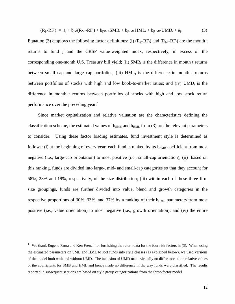
(Rjt-RFt) = aj + bjM(RMt-RFt) + bjSMBSMBt + bjHMLHMLt + bjUMDUMDt + ejt. (3)

Equation (3) employs the following factor definitions: (i) (Rjt-RFt) and (RMt-RFt) are the month t

returns to fund j and the CRSP value-weighted index, respectively, in excess of the

corresponding one-month U.S. Treasury bill yield; (ii) SMBt is the difference in month t returns

between small cap and large cap portfolios; (iii) HMLt is the difference in month t returns

between portfolios of stocks with high and low book-to-market ratios; and (iv) UMDt is the

difference in month t returns between portfolios of stocks with high and low stock return

performance over the preceding year.4

Since market capitalization and relative valuation are the characteristics defining the

classification scheme, the estimated values of bSMB and bHML from (3) are the relevant parameters

to consider. Using these factor loading estimates, fund investment style is determined as

follows: (i) at the beginning of every year, each fund is ranked by its bSMB coefficient from most

negative (i.e., large-cap orientation) to most positive (i.e., small-cap orientation); (ii) based on

this ranking, funds are divided into large-, mid- and small-cap categories so that they account for

58%, 23% and 19%, respectively, of the size distribution; (iii) within each of these three firm

size groupings, funds are further divided into value, blend and growth categories in the

respective proportions of 30%, 33%, and 37% by a ranking of their bHML parameters from most

positive (i.e., value orientation) to most negative (i.e., growth orientation); and (iv) the entire

4 We thank Eugene Fama and Ken French for furnishing the return data for the four risk factors in (3). When using

the estimated parameters on SMB and HML to sort funds into style classes (as explained below), we used versions

of the model both with and without UMD. The inclusion of UMD made virtually no difference in the relative values

of the coefficients for SMB and HML and hence made no difference in the way funds were classified. The results

reported in subsequent sections are based on style group categorizations from the three-factor model.

13

sorting process, starting with a re-estimation of (3) for every available fund, is repeated each

January during the sample period as new funds satisfy the selection criteria.5

3.2. Descriptive Statistics

The top part of Table 1 summarizes the total number of funds in each style category for

every year of the sample period. With our assignment process, the earliest style category year

possible is 1981, with funds for this period having returns dating to January 1978. The final

column shows the steady increase during most of the period in the total number of funds

available; from 251 portfolios in 1981, the sample grew at an annual rate of about 6% to 1,142

funds in 2009. The bottom part of the display lists descriptive statistics for annual total return,

return standard deviation, assets under management, expense ratio, and portfolio turnover. The

reported figures confirm much of the conventional wisdom about investment style and fund

performance. For instance, value-oriented funds in the large-cap category produce average

annual returns that are consistently higher than those for growth-oriented portfolios, but only

marginally so for small-cap funds and not at all for mid-cap portfolios. Alternatively, controlling

for the book-to-market ratio, small-cap funds outperform large-cap funds by an average of

between 2.11 and 2.93% per year, albeit with higher total standard deviations. 5 The percentages used in this classification process reflect the actual style cell proportions for those funds in our

sample that Morningstar did classify during the 1992-2009 subperiod. To insure that this approach did not bias the

findings in the study, we also replicated all of our analysis after sorting fund style by two different schemes. First,

we classified funds into style groups each year according to the proportions that Morningstar employs for classifying

their sample: (70%, 20%, 10%) for the market capitalization dimension and equal weightings for the relative

valuation dimension. (Notice, however, that applying these proportions on an ex-post basis to a different sample

would be more likely to lead to an arbitrary outcome if the characteristics inherent in that sample did not

coincidentally match.) Second, for the subperiod starting in 1992, we also used Morningstar’s actual style group

assignments for the funds in our sample. Neither of these alternative classification schemes produces results that are

materially different in any way from those reported herein and they are available upon request; see also Chan et al.

(2002) for a variation on this style classification scheme.

14

These summary statistics also reveal that portfolios in different style categories appear to

be managed differently. Over the entire sample period, growth funds have higher turnover ratios

than value funds (e.g., SG turnover exceeds SV turnover by 114.94 to 78.79 percent) and large-

cap funds have lower turnover ratios than small cap funds (e.g., LG turnover is 20.74 percentage

points lower than SG turnover). Additionally, small-cap and growth funds have higher expense

ratios than large-cap and value funds, respectively. Finally, large-cap funds consistently hold

more assets than small-cap funds.

These results imply that it may be difficult to compare directly the return performance of

two funds with contrasting investment styles. Fund investment prowess is more appropriately

viewed on a relative basis within style categories; this is the tournament approach that Brown et

al. (1996) adopt, where a manager’s performance and compensation are determined compared to

peers within a style class. Of course, this industry practice is driven by investors who

concentrate on a fund’s past total returns when making their investment decisions (e.g., Sirri and

Tufano (1998)). Consequently, in the subsequent analysis, we consider the role that investment

style volatility exerts on fund performance in the context of the nine style tournaments defined

by the size- and valuation ratio-based categories.

3.3. Style Volatility Behavior

For this initial analysis, we calculate fund HSV values for each year for all nine style

classes, using returns for the prior three years. Funds are then rank ordered and sorted into low

style volatility and high style volatility subsamples by median value for the objective class.

Table 2 summarizes the characteristics of funds split into these style volatility bins and lists sub-

group median values for the following statistics: HSV, end-of-year total net assets, peer group

ranking (i.e., the fund’s relative position in the annual performance tournament, based on total

15

return), annual total return, return standard deviation, annual tracking error (TE) relative to a

style-specific benchmark portfolio, portfolio turnover, and expense ratio.6 To produce the

reported numbers, we sort the funds annually into HSV groups to produce the base levels of the

various statistics and these values are then averaged to produce the display.

The findings indicate that large-cap funds demonstrate less investment style volatility than

do small- or mid-cap funds. For instance, the median HSV value for the low volatility portion of

the three large-cap style categories is 0.47. By contrast, the low-style volatility portions of the

small- and mid-cap objectives yield a median HSV value of 0.61. Comparable results obtain for

the high-style volatility groupings: The median large-cap HSV is 0.86 with the analogous value

for the other two size-based categories being 1.03. Additionally, the median low-HSV fund

always has a lower tracking error to its benchmark than its high-HSV counterpart. Although not

shown, findings from the 1981-1994 and 1995-2009 subperiods confirm all of these patterns.

Table 2 also provides initial evidence supporting the conjecture that less style-volatile

funds are managed in a significantly different manner than more style-volatile ones. Based on a

simple comparison of median turnover ratios, it is apparent that low-HSV funds do less trading

than otherwise comparable high-HSV portfolios in all nine style groups. Further, low-HSV

funds also have lower average expense ratios and appear to produce higher total and relative

returns for virtually all of the style categories. The median annual fund returns produced by low-

HSV funds are larger than those for high-HSV managers in eight of the nine style categories

(MG being the exception), but with lower return standard deviations in all nine cases.

6 We estimate a fund’s tracking error as the volatility over time of the difference between its return and that to the

style class benchmark using 36 months of past returns and the following style-specific indexes: Russell 1000-Value

(LV), Russell 1000-Blend (LB), Russell 1000-Growth (LG), Russell Mid-Cap-Value (MV), Russell Mid-Cap-Blend

(MB), Russell Mid-Cap-Growth (MG), Russell 2000-Value (SV), Russell 2000-Blend (SB), and Russell 2000-

Growth (SG). The return data for these indexes came directly from Frank Russell Company (now FTSE-Russell).

16

Additionally, the managers of less style-volatile portfolios produce a higher median style group

ranking in all nine style groups.

3.4. Relative Contributions to Style Volatility

The style volatility measure in (2) averages the standard deviations of the fund’s mean

ranking with respect to three style factors: market capitalization, book-to-market ratio, and return

momentum. Thus, for any fund on a given assessment date, it is possible to measure the overall

level of style volatility as well as the amount each characteristic contributes to the total. We

would not expect a priori that each style factor will add equally to a fund’s overall HSV score.

Instead, it is likely that active portfolio managers using style timing strategies may increase the

dispersion in their ranking to different factors at different points in time.

To understand this process better, for every fund j in our sample on each measurement date

t we calculate the proportion of HSV contributed by the c-th style characteristic as [σc,j,t ÷ (3 *

HSVj,t)], which is just the style factor-specific score in (1) divided by the numerator of (2). We

then calculate cross-sectional averages of these contribution proportions on a yearly basis from

1981 to 2009, based on the year-end values of σc,j,t and HSVj,t.

Figure 1 illustrates how the relative contributions to HSV from each of the three style

characteristics evolved over time. The most striking finding is the substantial role that return

momentum plays in determining the overall level of a fund’s investment style volatility. Indeed,

variation in the momentum factor contributes almost as much as the size and value-growth

factors combined. The numbers underlying the graph bear this out: The time-series average

contribution proportion for the momentum factor is 48.1% while the size and value-growth

factors account for 22.0% and 29.9%, respectively, of the variation in HSV. Further, the annual

contribution proportions for the momentum style characteristic range from 43.1% to 55.4%.

17

One potential explanation for this outcome is that fund managers are often more

constrained by investors with regard to the decisions they make on the size and value-growth

dimensions of their portfolios. Therefore, altering a portfolio by either of those two

characteristics is likely to be far more of a visible event than if the return momentum

characteristic is allowed to vary. Of course, the fact that momentum is the largest contributor to

HSV does not mean that it will be the most useful style factor in explaining future fund

performance, which is a topic we examine in the next section.

4. Main Empirical Results

4.1. Overall Tests

4.1.1. Panel Regression Results

Collectively, the first two hypotheses specified earlier hold that (i) the volatility of a fund’s

investment style will be negatively related to the manager’s ability to produce superior risk-

adjusted returns in the future, and (ii) this style volatility effect is distinct from the impact

associated with the persistence of past fund performance. To test this combined prediction, we

estimate a series of panel regression equations with the following methodology:

(i) Starting at the beginning of our sample period, for each available fund we estimate the

parameters of (3) using the previous 36 months of returns. This estimation produces the

intercept term—i.e., ALPHA—we use as our proxy for past abnormal investment

performance. The HSV statistic is calculated by (2) over this same 36-month window.

(ii) At this same point in time, we calculate each fund’s risk-adjusted return over the

subsequent n-month period. For this task, using a forward-looking alpha coefficient relative

to a factor model such as (3) with “stale” parameter estimates can lead to sub-optimal

inference; see Cremers et al. (2012). Instead, since fund complexes and managers act as if

they compete in more narrowly defined style-specific tournaments, we convert a fund’s total

18

return over a given horizon to a z-score by standardizing within the portfolio’s style

classification.7 We refer to this value as the fund’s risk-adjusted tournament return and it is

our primary measure of future performance.

(iii) We specify four values of n: one (i.e., the fund’s next month return), three (i.e., the

fund’s next quarter return), six (i.e., the fund’s next two-quarter return) and 12 (i.e., the

fund’s next year return). These performance statistics represent risk-adjusted future returns

because they are calculated over a different time period than the style volatility and past

performance variables we use to explain them. To create a complete time series for each

fund, we repeat the previous steps by sequentially rolling the 36-month estimation window

forward n months at a time, where the value for n once again defines the length of the future

return forecast period.

(iv) In separate estimations, we then regress the one-, three-, six- or 12-month tournament

returns on the prior levels of ALPHA and HSV using all available data for each sample fund.

To assess their combined influence on future risk-adjusted returns, we also consider an

interaction term defined as the product of ALPHA and HSV. In various forms of this

regression, we include the following control variables: portfolio turnover (TURN), fund size

7 We replicate our entire set of results using three separate measures of future risk-adjusted fund returns, which

differ primarily in how fund risk is estimated. Chiefly because of its out-of-sample nature, throughout the study we

report findings based on the following design: Each fund’s total return is normalized within its relevant style class

(i.e., tournament) by subtracting the return to its style-specific benchmark portfolio and then dividing this difference

by the cross-sectional standard deviation of the funds in that style class, or ( )

n)t1,...,(ts,

n)t1,...,(ts,b,n)t1,...,(ts,j, R - R

++

++++

σ. We also

estimate two alternative measures where (i) risk is measured by the historical standard deviation of Fund j’s returns

over the 36-month period ending just before month t, and (ii) Fund j’s historical standard deviation is indexed to the

historical standard deviation of the benchmark for style class s. Our main findings are invariant to these

adjustments, which are available upon request.

19

(TNA), measured by the assets under management at the end of the estimation period, and

fund expense ratio (EXPR).

(v) Each specification of these panel regressions is estimated with year fixed-effects to

control for unobserved heterogeneity in the cross-section of funds caused by time passing.

Table 3 reports results for these regressions. The findings in Panels A, B, C, and D use

one-, three-, six-, and 12-month future risk-adjusted returns as a dependent variable, respectively.

We estimate parameters for seven different combinations of the independent variables, starting

with a simple model involving ALPHA alone (Model 1), which provides a baseline analysis of

the persistence phenomenon. The positive coefficient values in all four panels of the display

indicate that relative performance did indeed persist throughout the sample period. This alpha

persistence effect proves to be reliable even though the return-generating model used to measure

risk-adjusted returns includes a return momentum factor, despite Carhart’s (1997) finding that

alpha persistence largely disappears when this exposure is considered directly.

The remaining six models in Table 3 (Models 2-7) then examine the role that investment

style volatility plays in predicting future risk-adjusted fund performance. Overall, the results

strongly support the conclusion that these two variables are inversely and meaningfully related.

The coefficients estimated for HSV are always in the predicted negative direction (i.e., higher

past style volatility, lower future risk-adjusted performance) and are virtually always statistically

significant. For instance, Model 2 tests the simplest form of the relationship between subsequent

returns and HSV. Across the four panels, all of the return forecast periods produce highly

significant coefficient values of the appropriate sign: -0.009 for one-month returns, -0.025 for

three-month returns, -0.031 for six-month returns, and -0.028 for 12-month returns.

20

Additionally, notice that like ALPHA, the influence of HSV appears to peak for the three- and

six-month future return prediction periods.8

The findings for the four variations of Model 3—which includes HSV with ALPHA as

regressors—show that the style volatility variable is not a simple surrogate for ALPHA. In fact,

the coefficient levels for HSV remain statistically significant and either do not change in value or

actually increase with the addition of the past performance metric. Further, there is some

evidence that the style volatility and persistence variables combine in a way that produces a

meaningful effect; the various coefficients for the [ALPHA*HSV] interaction term in Models 4

are negative but generally less significant and the inclusion of this term has virtually no impact

on the influence exerted by either ALPHA or HSV separately. Accordingly, these results

confirm the uniqueness of style volatility as a determinant of future risk-adjusted returns.

Models 5-7 explore these relationships further by controlling for other mitigating

influences. The results for Models 5-6 show that adding portfolio turnover (TURN) and fund

size (TNA) does nothing to diminish the magnitude of the style volatility variable. Therefore, it

also appears that HSV is not merely a proxy for TURN. Finally, the connection between style

volatility and future risk-adjusted performance is only slightly affected once fund expense ratios

are added as a regressor (i.e., Model 7), with the parameters on HSV diminishing in magnitude

but remaining statistically significant for all but the 12-month future returns. Viewed as a whole,

the findings in Table 3 provide strong support for the proposition that the volatility of a fund’s

investment style does impact its future performance in a distinctive manner.

8 To provide some economic intuition for these parameters, recall that the dependent variable is the fund’s net-of-

benchmark return divided by the cross-sectional standard deviation of the returns to all of the peer funds in the style

group. So, focusing on the 12-month forecast parameter of -0.028 and noting that the average cross-sectional style

group standard deviation is about 20%, this implies an increase in a fund’s style-adjusted annual excess return of 56

basis points (i.e., -0.028 x 20%) for each one standard deviation decline in the HSV measure.

21

4.1.2. Fama-MacBeth Cross-Sectional Results

Although the tests just presented control for time fixed effects, it is still possible that the

residuals are correlated across funds during a given period. To mitigate this concern, we adopt

the methodology of Fama and MacBeth (1973) to test for the roles that style volatility and

performance persistence play in predicting future returns on a cross-sectional basis. Specifically,

for every fund on a given month, we use the prior 36 months of data to calculate values of past

performance (ALPHA) and the style volatility score (HSV). Next, we compute risk-adjusted

tournament returns for each fund over the subsequent one-, three-, six-, and 12-month periods,

which then become the dependent variables in a four separate cross-sectional regressions in

which ALPHA, HSV and the other controls are the independent variables. Finally, repeating the

first two steps for a series of different months that are rolled forward on a periodic n-month basis

generates the requisite time series of parameter estimates.

For each of the respective sets of future returns, Panels A-D of Table 4 list averages of the

time series of these estimated coefficients, along with p-values based on the means of those

coefficients. All four panels confirm the general conclusions discussed above and underscore

that they are neither spurious nor driven by large samples. First, the positive correlation between

past and future risk-adjusted fund returns suggests the existence of performance persistence in

the fund sample. Second, there is also a strong inverse connection between a fund’s style

volatility and its future risk-adjusted performance, with the strongest relationship for three- and

six-month future returns. Third, [ALPHA*HSV] remains negative but becomes highly

insignificant and its inclusion does little to reduce the influence of the past performance and style

volatility variables taken separately. Fourth, TNA is still an unreliable explanatory variable,

whereas the coefficient on TURN remains significantly positive, albeit at attenuated levels.

22

Finally, the fund’s expense ratio is still strongly negatively correlated with future risk-adjusted

performance and this relationship dissipates the impact of ALPHA and HSV to a minor extent.

4.2. The Characteristics of Style Volatility and Fund Performance

Figure 1 illustrated that the three separate style characteristics—size, value-growth, and

momentum— are not represented equally in HSV statistic. Thus, it is possible that the volatility

contributions associated with these characteristics might also differ in how they correlate with

the fund’s future risk-adjusted returns. To examine this issue, we replicate the panel regression

analysis in Table 3 using three non-overlapping regressors associated with the style characteristic

volatility statistics (i.e., σc,j,t) defined in (1) that form the component parts of the aggregate HSV

measure. Table 5 summarizes these findings, listing the estimated parameters from an

appropriately modified version of Model 7 in Table 3 (i.e., the “full control” specification) for all

four forecast horizons. The findings show the dramatic difference that the source characteristic

makes in how style volatility impacts future fund performance. In particular, the overall negative

correlation between HSV and subsequent risk-adjusted returns is not a uniform result across the

coefficients reported for the component volatility source variables. For style volatility related to

market capitalization (i.e., σsize), the reported parameter values are negative and highly

statistically significant regardless of the return forecast period. For the value-growth component,

estimated coefficients remain negative for all four prediction periods, but are only statistically

reliable for the three-month forecast horizons. Conversely, when the return momentum

contribution is isolated, the relationship between style volatility and future performance is

completely insignificant.

The immediate implication of these findings is that when the volatility in the investment

style of a portfolio is driven primarily by the market capitalization factor, it leads to a significant

23

relative reduction in the fund’s risk-adjusted returns over periods ranging from one month to one

year into the future. Style volatility driven by the value-growth characteristic has a comparable

effect, although apparently not as reliable. On the other hand, style volatility borne of the

decision to alter the portfolio’s return momentum dimension does not lead to a diminution of

future relative performance. The surprising thing about this situation is that although the firm

size characteristic makes the smallest contribution to the style volatility statistic of the average

portfolio—the time-series mean of [σsize ÷ HSV] is just 22%—it is nevertheless an extremely

destructive force when it is the dominant source of variation for a specific fund. Variations in

the value-growth factor are similarly destructive to future performance but to a far lesser extent.

Finally, portfolios with wide variations in their return momentum characteristic, which is the

source of most style volatility, apparently do not suffer because of it.

5. Decomposing Style Volatility

5.1. Measuring Direct and Indirect Style Volatility Effects

A logical extension of the preceding analysis asks the following question: To what extent is

a portfolio’s level of style volatility related to direct managerial actions as opposed to changes

that might have occurred without his or her awareness? To address this issue, we extract from

HSV two supplementary measures that capture: (i) the direct style volatility that results from

explicit adjustments the manager makes to the portfolio’s holdings; and (ii) the indirect style

volatility in the portfolio that manifests implicitly whenever the style characteristics of the

existing set of holdings change over time.

To understand the difference between these direct and indirect components, notice that

managers who actively attempt to adjust the investment style of their portfolios can do so in two

ways. First, they can make security-specific trades which, while based on relative valuation

24

judgments, nevertheless have the effect of altering the aggregate style characteristics of the fund.

Second, managers can make trades in an attempt to time perceived rotations in the style factors

directly (e.g., increase holdings of large-cap stocks, decrease holdings of small-cap stocks).

Regardless of the reason, these explicit adjustments will be reflected in changes in the portfolio

share holdings over time which, assuming the characteristic rankings of stocks in the portfolio

remain fixed, become the source of any style variation that managers intended to implement.

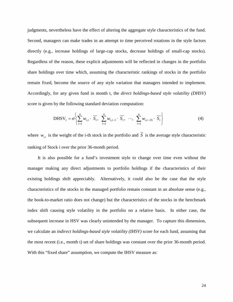
Accordingly, for any given fund in month t, the direct holdings-based style volatility (DHSV)

score is given by the following standard deviation computation:

⋅⋅⋅⋅⋅⋅= ∑ ∑ ∑= = =

−−

n

i

n

i

n

iitiitiiti SwSwSw

1 1 135,1,,t ,, , DHSV σ (4)

where tiw , is the weight of the i-th stock in the portfolio and S is the average style characteristic

ranking of Stock i over the prior 36-month period.

It is also possible for a fund’s investment style to change over time even without the

manager making any direct adjustments to portfolio holdings if the characteristics of their

existing holdings shift appreciably. Alternatively, it could also be the case that the style

characteristics of the stocks in the managed portfolio remain constant in an absolute sense (e.g.,

the book-to-market ratio does not change) but the characteristics of the stocks in the benchmark

index shift causing style volatility in the portfolio on a relative basis. In either case, the

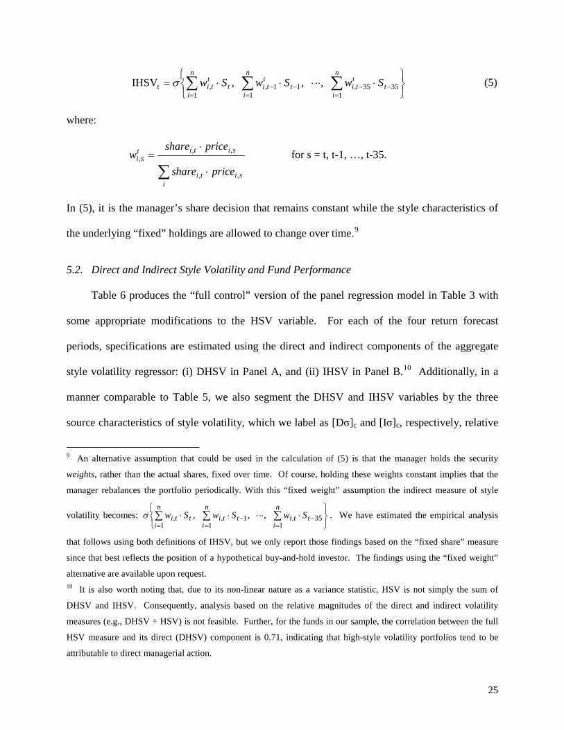
subsequent increase in HSV was clearly unintended by the manager. To capture this dimension,

we calculate an indirect holdings-based style volatility (IHSV) score for each fund, assuming that

the most recent (i.e., month t) set of share holdings was constant over the prior 36-month period.

With this “fixed share” assumption, we compute the IHSV measure as:

25

⋅⋅⋅⋅⋅⋅= ∑ ∑ ∑= = =

−−−−

n

i

n

i

n

it

ttit

ttit

tti SwSwSw

1 1 13535,11,,t ,,,IHSV σ (5)

where:

∑ ⋅

⋅=

isiti

sititsi

priceshare

pricesharew

,,

,,,

for s = t, t-1, …, t-35.

In (5), it is the manager’s share decision that remains constant while the style characteristics of

the underlying “fixed” holdings are allowed to change over time.9

5.2. Direct and Indirect Style Volatility and Fund Performance

Table 6 produces the “full control” version of the panel regression model in Table 3 with

some appropriate modifications to the HSV variable. For each of the four return forecast

periods, specifications are estimated using the direct and indirect components of the aggregate

style volatility regressor: (i) DHSV in Panel A, and (ii) IHSV in Panel B.10 Additionally, in a

manner comparable to Table 5, we also segment the DHSV and IHSV variables by the three

source characteristics of style volatility, which we label as [Dσ]c and [Iσ]c, respectively, relative

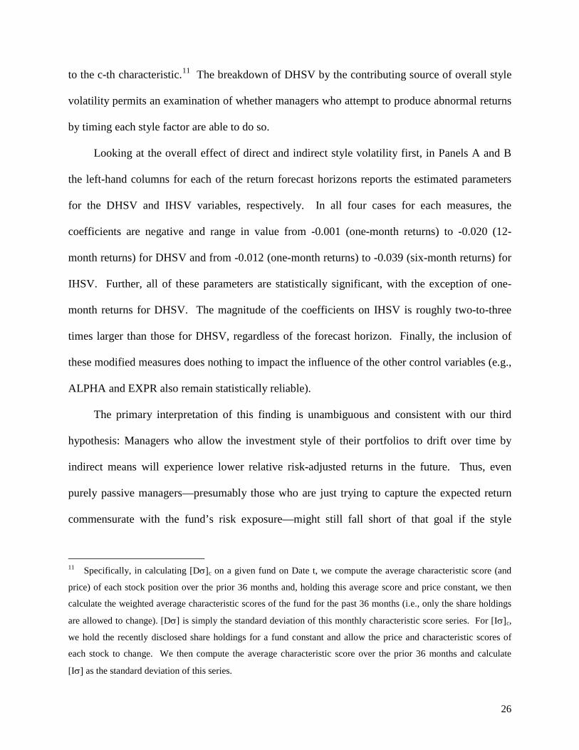
9 An alternative assumption that could be used in the calculation of (5) is that the manager holds the security

weights, rather than the actual shares, fixed over time. Of course, holding these weights constant implies that the

manager rebalances the portfolio periodically. With this “fixed weight” assumption the indirect measure of style

volatility becomes:

⋅⋅⋅⋅⋅⋅∑ ∑ ∑= = =

−−n

i

n

i

n

ittittitti SwSwSw

1 1 135,1,, ,,,σ . We have estimated the empirical analysis

that follows using both definitions of IHSV, but we only report those findings based on the “fixed share” measure

since that best reflects the position of a hypothetical buy-and-hold investor. The findings using the “fixed weight”

alternative are available upon request. 10 It is also worth noting that, due to its non-linear nature as a variance statistic, HSV is not simply the sum of

DHSV and IHSV. Consequently, analysis based on the relative magnitudes of the direct and indirect volatility

measures (e.g., DHSV ÷ HSV) is not feasible. Further, for the funds in our sample, the correlation between the full

HSV measure and its direct (DHSV) component is 0.71, indicating that high-style volatility portfolios tend to be

attributable to direct managerial action.

26

to the c-th characteristic.11 The breakdown of DHSV by the contributing source of overall style

volatility permits an examination of whether managers who attempt to produce abnormal returns

by timing each style factor are able to do so.

Looking at the overall effect of direct and indirect style volatility first, in Panels A and B

the left-hand columns for each of the return forecast horizons reports the estimated parameters

for the DHSV and IHSV variables, respectively. In all four cases for each measures, the

coefficients are negative and range in value from -0.001 (one-month returns) to -0.020 (12-

month returns) for DHSV and from -0.012 (one-month returns) to -0.039 (six-month returns) for

IHSV. Further, all of these parameters are statistically significant, with the exception of one-

month returns for DHSV. The magnitude of the coefficients on IHSV is roughly two-to-three

times larger than those for DHSV, regardless of the forecast horizon. Finally, the inclusion of

these modified measures does nothing to impact the influence of the other control variables (e.g.,

ALPHA and EXPR also remain statistically reliable).

The primary interpretation of this finding is unambiguous and consistent with our third

hypothesis: Managers who allow the investment style of their portfolios to drift over time by

indirect means will experience lower relative risk-adjusted returns in the future. Thus, even

purely passive managers—presumably those who are just trying to capture the expected return

commensurate with the fund’s risk exposure—might still fall short of that goal if the style

11 Specifically, in calculating [Dσ]c on a given fund on Date t, we compute the average characteristic score (and

price) of each stock position over the prior 36 months and, holding this average score and price constant, we then

calculate the weighted average characteristic scores of the fund for the past 36 months (i.e., only the share holdings

are allowed to change). [Dσ] is simply the standard deviation of this monthly characteristic score series. For [Iσ]c,

we hold the recently disclosed share holdings for a fund constant and allow the price and characteristic scores of

each stock to change. We then compute the average characteristic score over the prior 36 months and calculate

[Iσ] as the standard deviation of this series.

27

characteristics of their existing holdings shift appreciably from month to month. This implies

that fund managers with no intention of trying to produce abnormal returns through security

selection or tactical allocation still need to maintain a stable and predictable investment style in

their portfolios to prevent a loss of value relative to their peers. Beyond that, the relative size of

the parameter estimates for the DHSV variable suggest that managers who do manipulate the

investment style of their portfolios directly are not as likely to impact future performance in an

adverse manner as those managers whose style volatility may be unintentional.

Given the findings from the previous section, we also consider whether the impact of the

direct and indirect components of style volatility vary by style component. To investigate this

possibility, the right-hand columns of each return forecast period in Table 6 list the estimated

coefficients for the set of [Dσ]c and [Iσ]c variables described earlier. By design, these parameters

measure how a manager’s direct and indirect manipulation of the fund’s investment style affects

future returns, disaggregated by the source of those adjustments. In fact, the results are quite

similar to those for the characteristic segmentation of the aggregate HSV measure in Table 5.

The firm size characteristic is negatively correlated with subsequent performance for both the

DHSV and IHSV decompositions, although this relationship is considerably stronger when we

look at the indirect component of style volatility. Thus, managers who attempt to outperform

expectations by either explicitly adjusting the firm size style characteristic in their portfolio or

allow that component to change implicitly for other reasons will substantially inhibit future

performance. By contrast, the coefficients for both ([Dσ]vg , [Iσ]vg) and ([Dσ]mom , [Iσ]mom) are

far less statistically reliable and occasionally assume insignificantly positive values. Therefore,

with certain exceptions (e.g., the six-month forecast horizon), alterations in the other two style

28

characteristics—whether intended or not—seem to have little impact on the portfolio’s future

risk-adjusted performance.

6. Additional Robustness Tests

6.1. Style Volatility and the Role of Active Security Selection

Cremers and Petajisto (2009) introduce a measure of how managers intentionally

manipulate their portfolio weights to be different than those in the benchmark index. Their

Active Share (AS) statistic for fund j at month t is calculated for the N securities in the investable

universe as:

w- w 21 AS

N

1 iti,Index,ti,j,tj, ∑

=

= (6)

By construction, AS should capture the part of HSV related to deliberate security selection

strategies. Although our earlier findings show that indirect style volatility turns out to be the

most important predictor of future fund performance, it nevertheless may be the case that HSV

simply mimics the explanatory power of AS.

To see if this is true, we replicate the full version of our main panel regression using AS as

an additional control variable. Specifically, in addition to the Russell index return data described

earlier, we obtain the requisite index holdings data (i.e., constituent securities and investment

weights) from 1980 to 2009 from the Frank Russell Company. We then compute the AS measure

relative to the style group-specific indexes following equation (6).12 These regression results are

summarized in Table 7. The most important thing to note is that the coefficients on the overall

HSV variable remain negative for all four prediction intervals and are statistically significant for

all but the 12-month future returns. In fact, in comparison to the baseline findings presented in 12 Holdings data are not available for the Mid-Cap Value (MV), Mid-Cap Blend (MB), and Mid-Cap Growth (MG)

style indexes, which reduces slightly the sample size relative to the analysis reported previously.

29

Table 3, it is clear that the magnitude of the contribution of HSV is not diminished at all by

including AS as a regressor, which can also be said for the other controls such as ALPHA and

EXPR. Therefore, we can conclude that HSV is indeed a distinctive explanatory factor relative

to the information contained in the active selection variable alone.

6.2. An Alternative Style Classification Method

As explained in Section 3, we chose the factor loading-based method of classifying funds

into nine investment style categories due to its consistency with both market practice and past

academic research (e.g., Chan et al. (2002)). However, it is useful to consider the extent to

which our previous findings could be sensitive to these style classification definitions. While

some of the previous robustness checks suggest that modifications within the factor loading-

based scheme make no difference, it is nevertheless possible that a completely separate

alternative to the present style classification system might.

For instance, rather than using the estimated factor betas from (3), a fund’s style could also

be inferred directly from characteristics of its portfolio holdings. Once again relying on the

procedure developed in Kacpercyzk et al. (2005), for each fund in our sample at a given point in

time, we use the most recently reported set of holdings to calculate the average characteristic

score to each of the three style characteristics (i.e., market capitalization, book-to-market ratio,

and return momentum). Dividing the range of scores for each characteristic into terciles, we then

use a (3 x 3 x 3) sorting process to place each fund into its appropriate style category “bin” for

the purpose of normalizing its future risk-adjusted return measures. While this holdings-based

classification procedure using three style characteristics is not typical of how investment style is

categorized within the mutual fund industry, it is somewhat more analogous to how we define

our style volatility measure.

30

To see whether this alternative classification approach impacted our style volatility

measure’s ability to predict future risk-adjusted returns, we once again replicate the full version

of our main panel regression with the amended process. The results, which are listed in Table 8,

show that the alternative classification scheme had little overall effect on HSV’s importance as

an explanatory variable. As with the findings just described when the AS measure was included

as a control variable, the estimated coefficients for HSV remain negative for each of the four

future return prediction periods and statistically significant in all but the 12-month interval.

Further, none of the explanatory factors appear to have been affected by the alternative

categorization process (with the exception of TNA, which is now statistically significant for the

three shortest future return prediction periods). Thus, how a fund’s investment style is classified

does not appear to be the issue responsible for our original conclusions.

6.3. A Returns-Based Style Volatility Measure

We have emphasized throughout the study that our HSV measure of style volatility is based

on an examination of how the portfolio holdings in a mutual fund change over time. The implicit

assumption in this choice is that a style volatility measure based on portfolio returns rather than

holdings would not be as informative in that it would, at best, represent the “fingerprints” of the

manager’s decision-making prowess. On the other hand, returns can typically be measured over

much shorter time periods than holdings (e.g., daily) and more currently, which is a great

advantage to an investor trying to discriminate between the actual and self-reported style of a

given fund.

As a final robustness check, we examine whether the relationship between the

predictability of a portfolio’s investment style and its future performance obtains when using a

returns-based measure of style volatility instead of HSV. As Ammann and Zimmerman (2001)

31

note, the tracking error (TE) statistic is a natural way to use fund returns for this purpose, since

TE measures the variance of the return differential between a fund and its style-specific index.

Accordingly, at each point during the 1981-2009 sample period when we measure HSV, we also

calculate the portfolio’s TE statistic using the prior 36 months of return data. We then replicate

the complete analysis in Section 4 using TE as our style volatility measure in lieu of HSV. Table

9 presents a condensed version of these findings, again reporting the estimated coefficients for

the unconditional panel regression model containing the full set of controls.

Before discussing the findings, it is worth mentioning that the unconditional correlation

coefficient, aggregated cross-sectionally and across time, between HSV and TE is 0.5796. Thus,

we would expect the two measures to provide comparable, but not necessarily exact, results

when used as regressors in the fund performance forecast equation. Generally speaking, that is

exactly what the findings indicate. The coefficient on TE is significantly negative for all four

return forecast periods (including the 12-month horizon), which is consistent with the holding-

based results in that funds with a greater degree of past variability relative to their style

benchmark produce lower risk-adjusted returns in the future. An interpretation of the additional

control variables—especially ALPHA—also remains the same, as does the significantly negative

coefficient on the interaction term between ALPHA and TE. Consequently, the relationship

between a fund’s style volatility and future investment performance is not likely to be an artifact

of how the former variable is measured.

7. Economic Significance

To assess the economic significance of style volatility investing, we ask the following

question: Controlling for portfolio expenses and past performance, would investors be able to

exploit the return differential (if any) generated by less style-volatile portfolios versus more

32

style-volatile ones? We calculate the returns to several hypothetical portfolios sorted by

combinations of HSV, ALPHA, and EXPR. Beginning in January 1981, funds are divided into

one of two portfolios according to high and low values of the relevant sorting variables. These

portfolios are then rebalanced on a quarterly basis and investment performance statistics are

calculated through December 2009.

Table 10 documents the investment performance for six different pairs of portfolios. For

the first three of these portfolio pairs, funds are defined using just one of the sorting variables at

a time. This allows for a comparison of the differential impact that expense ratios, past

performance, and style volatility have when considered separately. The next two—[Lo EXPR,

Lo HSV] vs. [Hi EXPR, Hi HSV] and [Hi ALPHA, Lo HSV] vs. [Lo ALPHA, Hi HSV]—

provide comparisons of the synergies that exist when investors select managers that have either

low expense ratios or superior past performance along with a less style-volatile investment

approach. The final comparison examines the difference between [Lo EXPR, Hi ALPHA, Lo

HSV] and [Hi EXPR, Lo ALPHA, Hi HSV] managers who control for all three factors. In all

cases, high and low values of the sorting variables were defined by the upper and lower quartiles

of the respective distributions.

Without regard to past performance or style volatility issues, investing with managers who

run low-expense portfolios generates an annual return premium of 102 basis points (i.e., 10.91%

vs. 9.89%) and with a lower level of portfolio standard deviation. Further, investments based on

just past fund performance levels show an even more pronounced increase in annual return (i.e.,

11.47% to 9.24%) with a roughly comparable level of return standard deviation. Finally,

portfolios sorted unconditionally on the style volatility variable produce a 90 basis point return

premium for the Lo HSV investment, but with a risk level that was almost 60 basis points lower

33

than that for the Hi HSV portfolio. The comparative Sharpe ratios listed in the last column are

always larger for the respective upper quartile sort, showing that lower expense, higher past

performance, and less style volatile investments always outperformed their counterparts on a

risk-adjusted basis.13

The last three pair-wise comparisons document how the performance advantage associated

with the style volatility decision is embellished by managers with low expense, high past

performance operations. When Lo HSV and Hi HSV portfolios are modified to include extreme

values of ALPHA in the sorting procedure, the return premium increases from 90 basis points to

165 basis points (i.e., 11.08% vs. 9.43%). The synergy between EXPR and HSV is larger still;

adding this variable increases the Lo HSV vs. Hi HSV return premium from 90 to 268 basis

points. Lastly, when funds are sorted on all three variables, the result is a return differential of

344 basis points with a reduction in overall risk. As before, the Sharpe ratios for each of the Lo

HSV-based portfolios exceed those for the comparable Hi HSV portfolios by a sizeable margin.

The main conclusion implied by these findings is that each of the contributions of a fund

manager that we consider—running a low-expense operation, demonstrating superior

performance, and managing in a low style volatility manner—appears to have the potential to

benefit investors. Beyond the independent contributions they might make, there also appears to

be a considerable amount of synergy possible between these effects. Of course, given that the

benefits of investing with managers who control their expense ratios and persistently produce

13 Sharpe ratios are calculated for each portfolio as the difference between its average annual return and the average

annual risk-free rate divided by the portfolio’s annualized standard deviation. The average annual risk-free rate for

1981-2009 is 5.32%, which is established by annualizing the average of the monthly Treasury bill yields listed in the

Fama-French database.

34

superior risk-adjusted returns are well documented, the extension provided by these results is to

offer some perspective on the economic consequences of the manager’s style volatility choice.

8. Concluding Comments

One of the more intriguing developments in professional asset management during the past

few decades has been the evolution in how a portfolio’s investment style is defined and the role

that this style decision plays in determining fund returns. While considerable effort has been put

toward establishing whether a manager’s selection of a particular set of style characteristics

influences performance, relatively little is known about whether the manager’s ability to

maintain that style mandate—whatever it may be—also has a significant impact on investment

returns.

Does investment style volatility matter? The results of this study strongly suggest that the

answer is “yes”. Using a new measure of style volatility linked to fund holdings, we test three

specific hypotheses related to this issue, namely that: (i) a negative relationship exists between

portfolio style volatility and future risk-adjusted performance, (ii) the relationship between style

volatility and future performance is separate and distinct from the roles played by past

performance and fund expenses, and (iii) the direct and indirect components of style volatility

will have different impacts on future performance. Based on a survivorship bias-free sample of

equity mutual funds drawn from nine distinct style groups over 1978-2009, the data provide

strong support for all three propositions under a wide variety of test conditions and alternative

possibilities.

First, the typical low-style volatility fund does indeed tend to produce higher risk-adjusted

returns over subsequent holding periods ranging from one month to one year into the future.

Second, we also confirm that the connection between style volatility and future fund returns is

35

distinct from—and of comparable magnitude to—those related to past performance (i.e., alpha),

fund turnover, fund size, and fund expense ratio. Third, both the direct and indirect components

of style volatility retain a strong negative connection to future performance, and the firm size

characteristic appears to be to predominant source of those relationships. Further, we also show

that the relationship between style volatility and future fund returns does not change appreciably

when a returns-based volatility metric replaces our holdings-based statistic. Finally, the style

volatility measure proved useful in forming trading strategies capable of generating measurable

levels of outperformance.

These findings evoke several implications and extensions. Most notably, it appears that the

ability for portfolio managers to sustain a preferred degree of predictability to their designated

investment styles is a valuable skill. In fact, maintaining a low and observable level of volatility

in their investment style is one of the ways in which superior managers can signal their prowess

to investors. Further, although our results do not negate the possibility that managers who follow

an explicit tactical style timing strategy can be successful, they do suggest that indirect style

volatility can lead to inferior relative performance; the decision to maintain a stable and

predictable style profile may be more useful in helping managers avoid chronically poor

performance than in creating an environment that fosters persistent superior relative returns. At

a minimum, it seems clear that style volatility is another element that must be factored into the

on-going debate of whether mutual fund performance is predictable over time.

36

REFERENCES

Alford, A., Jones, R., Winkelmann, K., 2003. A Spectrum Approach to Active Risk Budgeting, Journal of Portfolio Management 30, 49-60. Ammann, M., Zimmerman H., 2001. Tracking error and tactical asset allocation, Financial Analysts Journal 57, 32-43. Asness, C., Friedman, J., Krail, R., Liew, J., 2000. Style timing: Value versus growth, Journal of Portfolio Management 26, 50-60. Barberis, N., Shleifer, A., 2003. Style investing, Journal of Financial Economics 68, 161-191. Bogle, J., 1998. The implications of style analysis for mutual fund performance evaluation. Journal of Portfolio Management 24, 34-42. Brown, K., Harlow, V., Starks, L., 1996. Of tournaments and temptations: An analysis of managerial incentives in the mutual fund industry. Journal of Finance 51, 85-110. Brown, S., Goetzmann, W., 1995. Performance persistence. Journal of Finance 50, 679-698. Brown, S., Goetzmann, W. 1997. Mutual fund styles. Journal of Financial Economics 43, 373-399. Carhart, M., 1997. On persistence in mutual fund performance. Journal of Finance 52, 57-82. Capaul, C, Rawley, I., Sharpe, W., 1993. International value and growth stock returns. Financial Analysts Journal 49, 27-36. Chan, L., Chen, H., Lakonishok, J., 2002. On mutual fund investment styles. Review of Financial Studies 15, 1407-1437. Chan, L., Lakonishok, J., 2004. Value and growth investing: Review and update. Financial Analysts Journal 60, 71-86. Christopherson, J., Ferson, W., Glassman, D., 1998. Conditioning manager alphas on economic information: Another look at the persistence of performance. Review of Financial Studies 11, 111-142. Coggin, D., Fabozzi, F., Rahman, S., 1993. The investment performance of U.S. equity pension fund managers: An empirical investigation. Journal of Finance 48, 1039-1055. Cremers, M., Petajisto, A., 2009. How active is your fund manager?: A new measure that predicts performance. Review of Financial Studies 22 3329-3365.

37

Cremers, M., Petajisto, A., Zitzewitz, E., 2012. Should benchmark indices have alpha? Revisiting performance evaluation. Critical Finance Review 2, 1-48. Daniel, K., Grinblatt, M., Titman, S., Wermers, R., 1997. Measuring mutual fund performance with characteristic-based benchmarks. Journal of Finance 52, 1035-1058. Fama, E., French, K., 1993. Common risk factors in the returns on stocks and bonds. Journal of Financial Economics 33, 3-56. Fama, E., French, K., 1998. Value versus growth: The international evidence. Journal of Finance 53, 1975-1999. Fama, E., MacBeth, J., 1973. Risk, return, and equilibrium: Empirical tests. Journal of Political Economy 81, 607-636. Gil-Boaz, J., Ruiz-Verdu, P., 2009. The relation between price and performance in the mutual fund industry. Journal of Finance 64, 2153-2183. Grinblatt, M., Titman, S., 1992. The persistence of mutual fund performance. Journal of Finance 47, 1977-1984. Hendricks, D., Patel, J., Zeckhauser, R., 1993. Hot hands in mutual funds: Short-run persistence of relative performance. 1974-1988. Journal of Finance 48, 93-130. Herrmann, U., Scholz H., 2013. Short-term persistence in hybrid mutual fund performance: The role of style-shifting abilities. Journal of Banking and Finance 37, 2314-2328. Huang, J., Sialm, C., Zhang, H., 2011. Risk shifting and mutual fund performance. Review of Financial Studies 24, 2575-2616. Ibbotson, R., Patel, A., 2002. Do winners repeat with style? Working Paper, Yale University International Center for Finance. Kacperczyk, M., Sialm, C., Zheng, L., 2005. On the industry concentration of actively managed equity mutual funds. Journal of Finance 60, 1983-2011. Malkiel, B., 1995. Returns from investing in equity mutual funds: 1971 to 1991. Journal of Finance 50, 549-572. Meier, I., Rombouts, J., 2009. Style rotation and the performance persistence of mutual funds. Working Paper, HEC Montreal. Sirri, E., Tufano, P., 1998. Costly search and mutual fund flows. Journal of Finance 53, 1589-1622.

38

Swinkels, L., Tjong-a-Tjoe, L., 2007. Can mutual funds time investment styles? Journal of Asset Management 8, 123-132. Wahal, S., D. Yavuz, D., 2012. Style investing, comovement and return predictability. Journal of Financial Economics 107, 136-154. Wermers, R., 2012. A matter of style: The causes and consequences of style drift in institutional portfolios. Working Paper, University of Maryland.

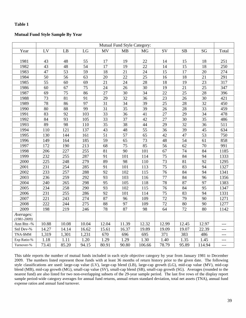
39

Table 1 Mutual Fund Style Sample By Year

Mutual Fund Style Category: Year LV LB LG MV MB MG SV SB SG Total

1981 43 48 55 17 19 22 14 15 18 251 1982 43 48 54 17 19 22 14 15 18 250 1983 47 53 59 18 21 24 15 17 20 274 1984 50 56 63 20 22 25 16 18 21 291 1985 55 60 69 21 24 28 18 19 23 317 1986 60 67 75 24 26 30 19 21 25 347 1987 69 75 86 27 30 34 22 25 28 396 1988 73 81 91 29 32 36 23 26 30 421 1989 78 86 97 31 34 39 25 28 32 450 1990 80 88 99 31 35 39 26 28 33 459 1991 83 92 103 33 36 41 27 29 34 478 1992 84 93 105 33 37 42 27 30 35 486 1993 89 98 110 35 38 44 29 32 36 511 1994 110 121 137 43 48 55 36 39 45 634 1995 130 144 161 51 57 65 42 47 53 750 1996 149 164 185 59 65 73 48 54 61 858 1997 172 190 213 68 75 85 56 62 70 991 1998 206 227 255 81 90 101 67 74 84 1185 1999 232 255 287 91 101 114 75 84 94 1333 2000 225 248 279 89 98 110 73 81 92 1295 2001 231 254 285 91 101 113 75 83 94 1327 2002 233 257 288 92 102 115 76 84 94 1341 2003 236 259 292 93 103 116 77 84 96 1356 2004 240 265 298 95 105 118 78 87 97 1383 2005 234 258 290 93 102 115 76 84 95 1347 2006 231 255 286 92 101 114 75 83 94 1331 2007 221 243 274 87 96 109 72 79 90 1271 2008 222 244 275 88 97 109 72 80 90 1277 2009 198 219 246 78 87 98 64 72 80 1142

Averages: (1981-2009)

Ann Rtn -% 10.88 10.08 10.04 12.04 11.39 12.32 12.99 12.45 12.97 --- Std Dev-% 14.27 14.14 16.62 15.61 16.37 19.89 19.09 19.07 22.39 --- TNA-$MM 1,319 1,301 1,231 670 696 695 371 383 486 --- Exp Ratio-% 1.18 1.11 1.20 1.29 1.29 1.30 1.40 1.35 1.45 --- Turnover-% 73.41 85.20 94.15 80.91 90.80 106.66 78.79 95.89 114.94 --- This table reports the number of mutual funds included in each style objective category by year from January 1981 to December 2009. The numbers listed represent those funds with at least 36 months of return history prior to the given date. The following style classifications are used: large-cap value (LV), large-cap blend (LB), large-cap growth (LG), mid-cap value (MV), mid-cap blend (MB), mid-cap growth (MG), small-cap value (SV), small-cap blend (SB), small-cap growth (SG). Averages (rounded to the nearest fund) are also listed for two non-overlapping subsets of the 29-year sample period. The last five rows of the display report sample period-wide category averages for annual fund returns, annual return standard deviation, total net assets (TNA), annual fund expense ratios and annual fund turnover.

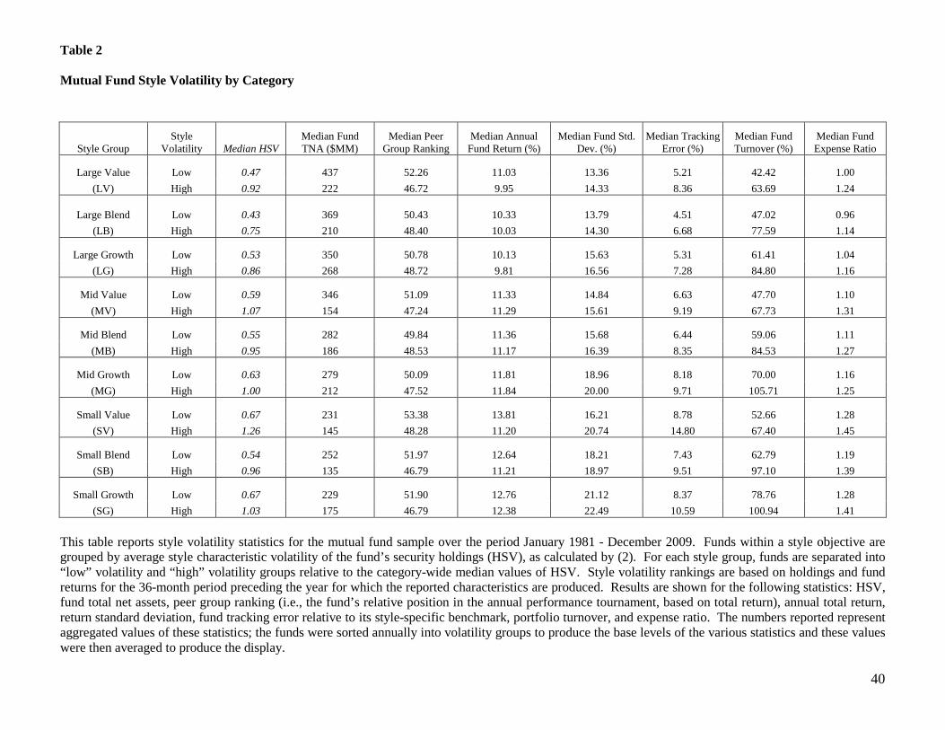
40

Table 2 Mutual Fund Style Volatility by Category

Style Group Style

Volatility Median HSV Median Fund TNA ($MM)

Median Peer Group Ranking

Median Annual Fund Return (%)

Median Fund Std. Dev. (%)

Median Tracking Error (%)

Median Fund Turnover (%)

Median Fund Expense Ratio

Large Value Low 0.47 437 52.26 11.03 13.36 5.21 42.42 1.00 (LV) High 0.92 222 46.72 9.95 14.33 8.36 63.69 1.24

Large Blend Low 0.43 369 50.43 10.33 13.79 4.51 47.02 0.96

(LB) High 0.75 210 48.40 10.03 14.30 6.68 77.59 1.14

Large Growth Low 0.53 350 50.78 10.13 15.63 5.31 61.41 1.04 (LG) High 0.86 268 48.72 9.81 16.56 7.28 84.80 1.16

Mid Value Low 0.59 346 51.09 11.33 14.84 6.63 47.70 1.10 (MV) High 1.07 154 47.24 11.29 15.61 9.19 67.73 1.31

Mid Blend Low 0.55 282 49.84 11.36 15.68 6.44 59.06 1.11 (MB) High 0.95 186 48.53 11.17 16.39 8.35 84.53 1.27

Mid Growth Low 0.63 279 50.09 11.81 18.96 8.18 70.00 1.16 (MG) High 1.00 212 47.52 11.84 20.00 9.71 105.71 1.25

Small Value Low 0.67 231 53.38 13.81 16.21 8.78 52.66 1.28 (SV) High 1.26 145 48.28 11.20 20.74 14.80 67.40 1.45

Small Blend Low 0.54 252 51.97 12.64 18.21 7.43 62.79 1.19 (SB) High 0.96 135 46.79 11.21 18.97 9.51 97.10 1.39

Small Growth Low 0.67 229 51.90 12.76 21.12 8.37 78.76 1.28 (SG) High 1.03 175 46.79 12.38 22.49 10.59 100.94 1.41

This table reports style volatility statistics for the mutual fund sample over the period January 1981 - December 2009. Funds within a style objective are grouped by average style characteristic volatility of the fund’s security holdings (HSV), as calculated by (2). For each style group, funds are separated into “low” volatility and “high” volatility groups relative to the category-wide median values of HSV. Style volatility rankings are based on holdings and fund returns for the 36-month period preceding the year for which the reported characteristics are produced. Results are shown for the following statistics: HSV, fund total net assets, peer group ranking (i.e., the fund’s relative position in the annual performance tournament, based on total return), annual total return, return standard deviation, fund tracking error relative to its style-specific benchmark, portfolio turnover, and expense ratio. The numbers reported represent aggregated values of these statistics; the funds were sorted annually into volatility groups to produce the base levels of the various statistics and these values were then averaged to produce the display.

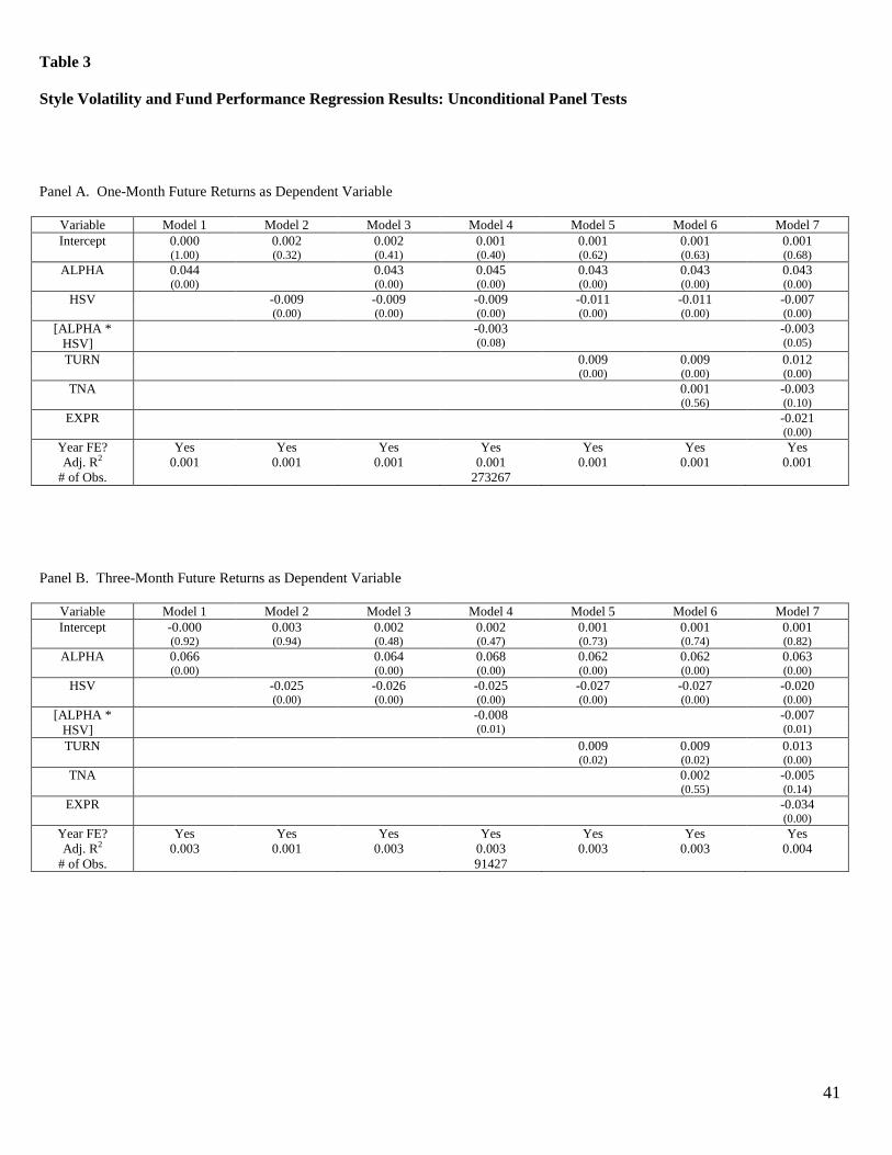
41

Table 3 Style Volatility and Fund Performance Regression Results: Unconditional Panel Tests

Panel A. One-Month Future Returns as Dependent Variable

Variable Model 1 Model 2 Model 3 Model 4 Model 5 Model 6 Model 7 Intercept 0.000 0.002 0.002 0.001 0.001 0.001 0.001

(1.00) (0.32) (0.41) (0.40) (0.62) (0.63) (0.68) ALPHA 0.044 0.043 0.045 0.043 0.043 0.043

(0.00) (0.00) (0.00) (0.00) (0.00) (0.00) HSV -0.009 -0.009 -0.009 -0.011 -0.011 -0.007

(0.00) (0.00) (0.00) (0.00) (0.00) (0.00) [ALPHA * -0.003 -0.003

HSV] (0.08) (0.05) TURN 0.009 0.009 0.012

(0.00) (0.00) (0.00) TNA 0.001 -0.003

(0.56) (0.10) EXPR -0.021

(0.00) Year FE? Adj. R2

# of Obs.

Yes 0.001

Yes 0.001

Yes 0.001

Yes 0.001

273267

Yes 0.001

Yes 0.001

Yes 0.001

Panel B. Three-Month Future Returns as Dependent Variable

Variable Model 1 Model 2 Model 3 Model 4 Model 5 Model 6 Model 7 Intercept -0.000 0.003 0.002 0.002 0.001 0.001 0.001

(0.92) (0.94) (0.48) (0.47) (0.73) (0.74) (0.82) ALPHA 0.066 0.064 0.068 0.062 0.062 0.063

(0.00) (0.00) (0.00) (0.00) (0.00) (0.00) HSV -0.025 -0.026 -0.025 -0.027 -0.027 -0.020

(0.00) (0.00) (0.00) (0.00) (0.00) (0.00) [ALPHA * -0.008 -0.007

HSV] (0.01) (0.01) TURN 0.009 0.009 0.013

(0.02) (0.02) (0.00) TNA 0.002 -0.005

(0.55) (0.14) EXPR -0.034

(0.00) Year FE? Adj. R2

# of Obs.

Yes 0.003

Yes 0.001

Yes 0.003

Yes 0.003 91427

Yes 0.003

Yes 0.003

Yes 0.004

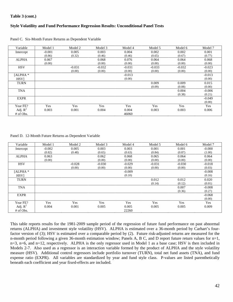
42

Table 3 (cont.) Style Volatility and Fund Performance Regression Results: Unconditional Panel Tests Panel C. Six-Month Future Returns as Dependent Variable

Variable Model 1 Model 2 Model 3 Model 4 Model 5 Model 6 Model 7 Intercept -0.001 0.005 0.003 0.004 0.002 0.002 0.001

(0.86) (0.32) (0.46) (0.46) (0.65) (0.67) (0.77) ALPHA 0.067 0.068 0.076 0.064 0.064 0.068

(0.00) (0.00) (0.00) (0.00) (0.00) (0.00) HSV -0.031 -0.032 -0.031 -0.033 -0.032 -0.023

(0.00) (0.00) (0.00) (0.00) (0.00) (0.00) [ALPHA * -0.013 -0.013

HSV] (0.00) (0.00) TURN 0.009 0.009 0.015

(0.09) (0.08) (0.00) TNA 0.004 -0.006

(0.38) (0.21) EXPR -0.049

(0.00) Year FE? Adj. R2

# of Obs.

Yes 0.003

Yes 0.001

Yes 0.004

Yes 0.004 46060

Yes 0.003

Yes 0.003

Yes 0.006

Panel D. 12-Month Future Returns as Dependent Variable

Variable Model 1 Model 2 Model 3 Model 4 Model 5 Model 6 Model 7 Intercept -0.002 0.005 0.003 0.003 0.001 0.001 -0.000

(0.82) (0.48) (0.65) (0.63) (0.84) (0.87) (1.00) ALPHA 0.063 0.062 0.068 0.065 0.064 0.064

(0.00) (0.00) (0.00) (0.00) (0.00) (0.00) HSV -0.028 -0.030 -0.029 -0.031 -0.030 -0.018

(0.00) (0.00) (0.00) (0.00) (0.00) (0.03) [ALPHA * -0.009 -0.008

HSV] (0.10) (0.16) TURN 0.012 0.012 0.020

(0.14) (0.12) (0.01) TNA 0.007 -0.008

(0.36) (0.27) EXPR -0.068

(0.00) Year FE? Adj. R2

# of Obs.

Yes 0.004

Yes 0.001

Yes 0.005

Yes 0.005 22260

Yes 0.005

Yes 0.005

Yes 0.009

This table reports results for the 1981-2009 sample period of the regression of future fund performance on past abnormal returns (ALPHA) and investment style volatility (HSV). ALPHA is estimated over a 36-month period by Carhart’s four-factor version of (3); HSV is estimated over a comparable period by (2). Future risk-adjusted returns are measured for the n-month period following a given 36-month estimation window; Panels A, B C, and D report future return values for n=1, n=3, n=6, and n=12, respectively. ALPHA is the only regressor used in Model 1 as a base case; HSV is then included in Models 2-7. Also used as a regressor is an interaction variable formed by the product of ALPHA and the style volatility measure (HSV). Additional control regressors include portfolio turnover (TURN), total net fund assets (TNA), and fund expense ratio (EXPR). All variables are standardized by year and fund style class. P-values are listed parenthetically beneath each coefficient and year fixed-effects are included.

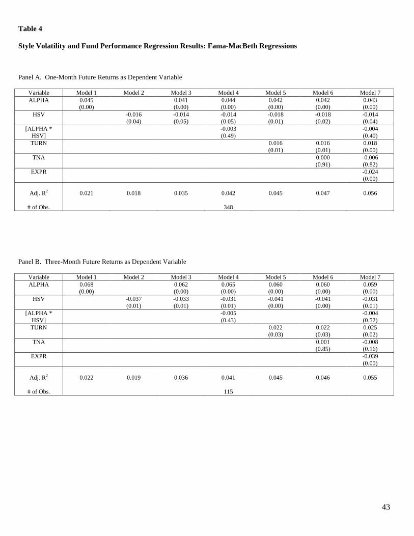
43

Table 4 Style Volatility and Fund Performance Regression Results: Fama-MacBeth Regressions Panel A. One-Month Future Returns as Dependent Variable

Variable Model 1 Model 2 Model 3 Model 4 Model 5 Model 6 Model 7 ALPHA 0.045 0.041 0.044 0.042 0.042 0.043

(0.00) (0.00) (0.00) (0.00) (0.00) (0.00) HSV -0.016 -0.014 -0.014 -0.018 -0.018 -0.014

(0.04) (0.05) (0.05) (0.01) (0.02) (0.04) [ALPHA * -0.003 -0.004

HSV] (0.49) (0.40) TURN 0.016 0.016 0.018

(0.01) (0.01) (0.00) TNA 0.000 -0.006

(0.91) (0.82) EXPR -0.024

(0.00)

Adj. R2

# of Obs.

0.021

0.018

0.035

0.042

348

0.045

0.047

0.056

Panel B. Three-Month Future Returns as Dependent Variable

Variable Model 1 Model 2 Model 3 Model 4 Model 5 Model 6 Model 7 ALPHA 0.068 0.062 0.065 0.060 0.060 0.059

(0.00) (0.00) (0.00) (0.00) (0.00) (0.00) HSV -0.037 -0.033 -0.031 -0.041 -0.041 -0.031

(0.01) (0.01) (0.01) (0.00) (0.00) (0.01) [ALPHA * -0.005 -0.004

HSV] (0.43) (0.52) TURN 0.022 0.022 0.025

(0.03) (0.03) (0.02) TNA 0.001 -0.008

(0.85) (0.16) EXPR -0.039

(0.00)

Adj. R2

# of Obs.

0.022

0.019

0.036

0.041

115

0.045

0.046

0.055

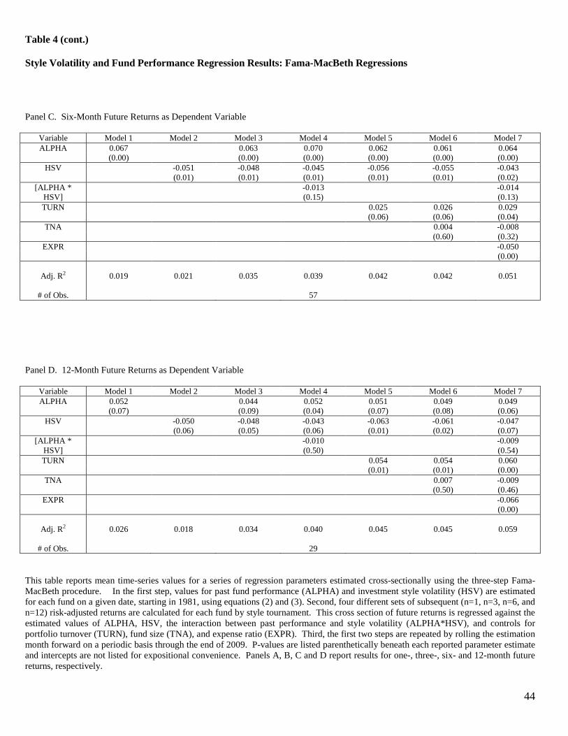
44

Table 4 (cont.) Style Volatility and Fund Performance Regression Results: Fama-MacBeth Regressions

Panel C. Six-Month Future Returns as Dependent Variable

Variable Model 1 Model 2 Model 3 Model 4 Model 5 Model 6 Model 7 ALPHA 0.067 0.063 0.070 0.062 0.061 0.064

(0.00) (0.00) (0.00) (0.00) (0.00) (0.00) HSV -0.051 -0.048 -0.045 -0.056 -0.055 -0.043

(0.01) (0.01) (0.01) (0.01) (0.01) (0.02) [ALPHA * -0.013 -0.014

HSV] (0.15) (0.13) TURN 0.025 0.026 0.029

(0.06) (0.06) (0.04) TNA 0.004 -0.008

(0.60) (0.32) EXPR -0.050

(0.00)

Adj. R2

# of Obs.

0.019

0.021

0.035

0.039

57

0.042

0.042

0.051

Panel D. 12-Month Future Returns as Dependent Variable

Variable Model 1 Model 2 Model 3 Model 4 Model 5 Model 6 Model 7 ALPHA 0.052 0.044 0.052 0.051 0.049 0.049

(0.07) (0.09) (0.04) (0.07) (0.08) (0.06) HSV -0.050 -0.048 -0.043 -0.063 -0.061 -0.047

(0.06) (0.05) (0.06) (0.01) (0.02) (0.07) [ALPHA * -0.010 -0.009

HSV] (0.50) (0.54) TURN 0.054 0.054 0.060

(0.01) (0.01) (0.00) TNA 0.007 -0.009

(0.50) (0.46) EXPR -0.066

(0.00)

Adj. R2

# of Obs.

0.026

0.018

0.034

0.040

29

0.045

0.045

0.059

This table reports mean time-series values for a series of regression parameters estimated cross-sectionally using the three-step Fama-MacBeth procedure. In the first step, values for past fund performance (ALPHA) and investment style volatility (HSV) are estimated for each fund on a given date, starting in 1981, using equations (2) and (3). Second, four different sets of subsequent (n=1, n=3, n=6, and n=12) risk-adjusted returns are calculated for each fund by style tournament. This cross section of future returns is regressed against the estimated values of ALPHA, HSV, the interaction between past performance and style volatility (ALPHA*HSV), and controls for portfolio turnover (TURN), fund size (TNA), and expense ratio (EXPR). Third, the first two steps are repeated by rolling the estimation month forward on a periodic basis through the end of 2009. P-values are listed parenthetically beneath each reported parameter estimate and intercepts are not listed for expositional convenience. Panels A, B, C and D report results for one-, three-, six- and 12-month future returns, respectively.

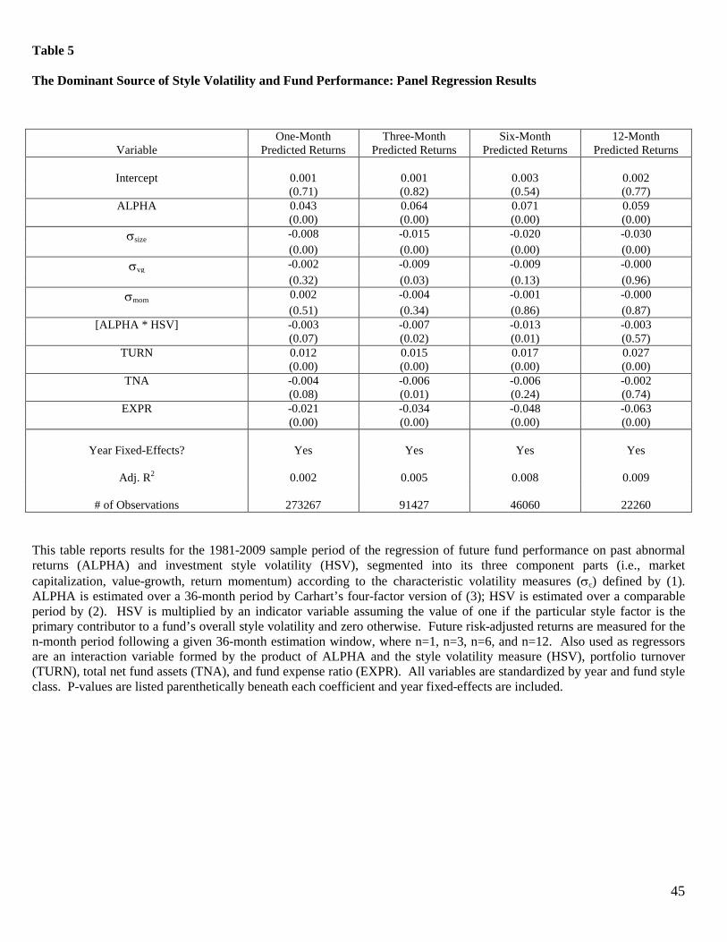
45

Table 5 The Dominant Source of Style Volatility and Fund Performance: Panel Regression Results

Variable

One-Month Predicted Returns

Three-Month Predicted Returns

Six-Month Predicted Returns

12-Month Predicted Returns

Intercept

0.001

0.001

0.003

0.002

(0.71) (0.82) (0.54) (0.77) ALPHA 0.043 0.064 0.071 0.059

(0.00) (0.00) (0.00) (0.00) σsize -0.008 -0.015 -0.020 -0.030

(0.00) (0.00) (0.00) (0.00) σvg -0.002 -0.009 -0.009 -0.000

(0.32) (0.03) (0.13) (0.96) σmom 0.002 -0.004 -0.001 -0.000

(0.51) (0.34) (0.86) (0.87) [ALPHA * HSV] -0.003 -0.007 -0.013 -0.003

(0.07) (0.02) (0.01) (0.57) TURN 0.012 0.015 0.017 0.027

(0.00) (0.00) (0.00) (0.00) TNA -0.004 -0.006 -0.006 -0.002

(0.08) (0.01) (0.24) (0.74) EXPR -0.021 -0.034 -0.048 -0.063

(0.00) (0.00) (0.00) (0.00)

Year Fixed-Effects?

Adj. R2

Yes

0.002

Yes

0.005

Yes

0.008

Yes

0.009

# of Observations

273267

91427

46060

22260

This table reports results for the 1981-2009 sample period of the regression of future fund performance on past abnormal returns (ALPHA) and investment style volatility (HSV), segmented into its three component parts (i.e., market capitalization, value-growth, return momentum) according to the characteristic volatility measures (σc) defined by (1). ALPHA is estimated over a 36-month period by Carhart’s four-factor version of (3); HSV is estimated over a comparable period by (2). HSV is multiplied by an indicator variable assuming the value of one if the particular style factor is the primary contributor to a fund’s overall style volatility and zero otherwise. Future risk-adjusted returns are measured for the n-month period following a given 36-month estimation window, where n=1, n=3, n=6, and n=12. Also used as regressors are an interaction variable formed by the product of ALPHA and the style volatility measure (HSV), portfolio turnover (TURN), total net fund assets (TNA), and fund expense ratio (EXPR). All variables are standardized by year and fund style class. P-values are listed parenthetically beneath each coefficient and year fixed-effects are included.

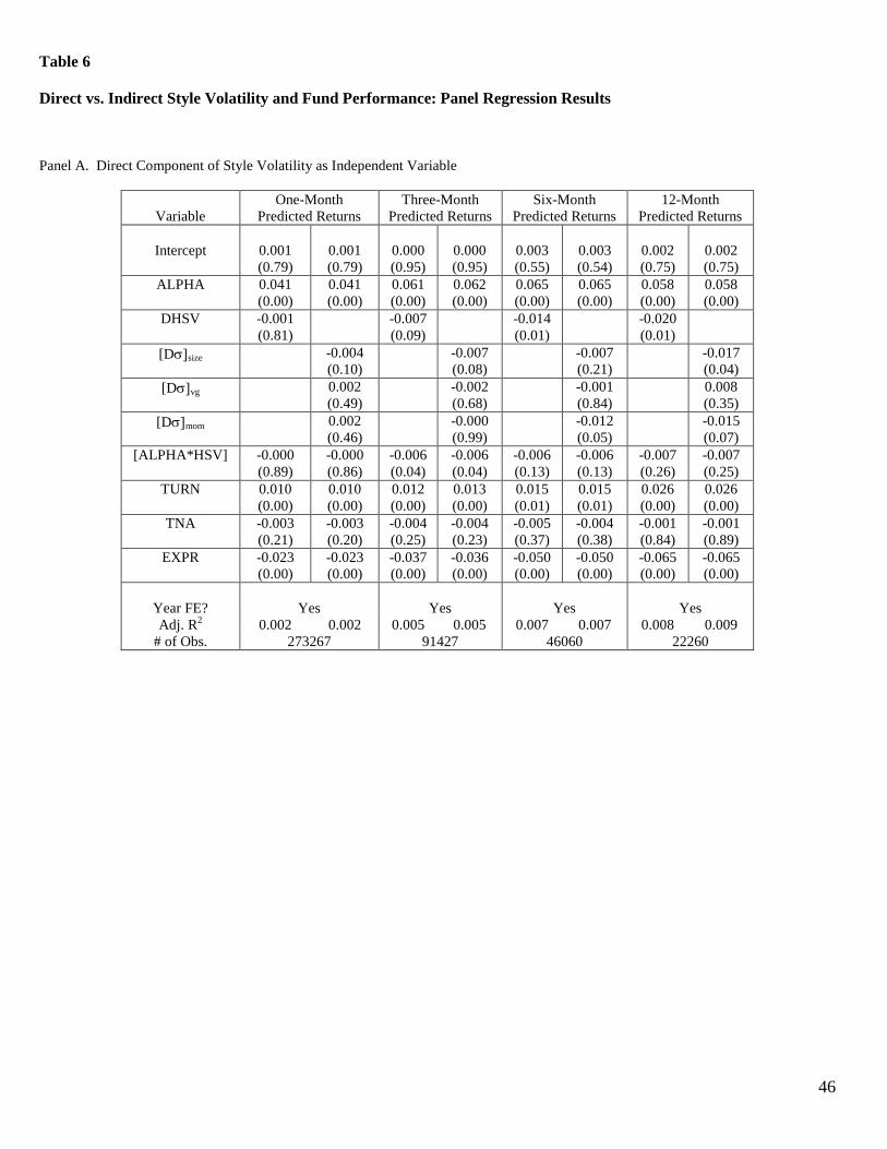
46

Table 6 Direct vs. Indirect Style Volatility and Fund Performance: Panel Regression Results Panel A. Direct Component of Style Volatility as Independent Variable

Variable

One-Month Predicted Returns

Three-Month Predicted Returns

Six-Month Predicted Returns

12-Month Predicted Returns

Intercept

0.001 (0.79)

0.001 (0.79)

0.000 (0.95)

0.000 (0.95)

0.003 (0.55)

0.003 (0.54)

0.002 (0.75)

0.002 (0.75)

ALPHA 0.041 (0.00)

0.041 (0.00)

0.061 (0.00)

0.062 (0.00)

0.065 (0.00)

0.065 (0.00)

0.058 (0.00)

0.058 (0.00)

DHSV -0.001 (0.81)

-0.007 (0.09)

-0.014 (0.01)

-0.020 (0.01)

[Dσ]size -0.004 (0.10)

-0.007 (0.08)

-0.007 (0.21)

-0.017 (0.04)

[Dσ]vg 0.002 (0.49)

-0.002 (0.68)

-0.001 (0.84)

0.008 (0.35)

[Dσ]mom 0.002 (0.46)

-0.000 (0.99)

-0.012 (0.05)

-0.015 (0.07)

[ALPHA*HSV] -0.000 (0.89)

-0.000 (0.86)

-0.006 (0.04)

-0.006 (0.04)

-0.006 (0.13)

-0.006 (0.13)

-0.007 (0.26)

-0.007 (0.25)

TURN 0.010 (0.00)

0.010 (0.00)

0.012 (0.00)

0.013 (0.00)

0.015 (0.01)

0.015 (0.01)

0.026 (0.00)

0.026 (0.00)

TNA -0.003 (0.21)

-0.003 (0.20)

-0.004 (0.25)

-0.004 (0.23)

-0.005 (0.37)

-0.004 (0.38)

-0.001 (0.84)

-0.001 (0.89)

EXPR -0.023 (0.00)

-0.023 (0.00)

-0.037 (0.00)

-0.036 (0.00)

-0.050 (0.00)

-0.050 (0.00)

-0.065 (0.00)

-0.065 (0.00)

Year FE?

Yes

Yes

Yes

Yes

Adj. R2 0.002 0.002 0.005 0.005 0.007 0.007 0.008 0.009 # of Obs. 273267 91427 46060 22260

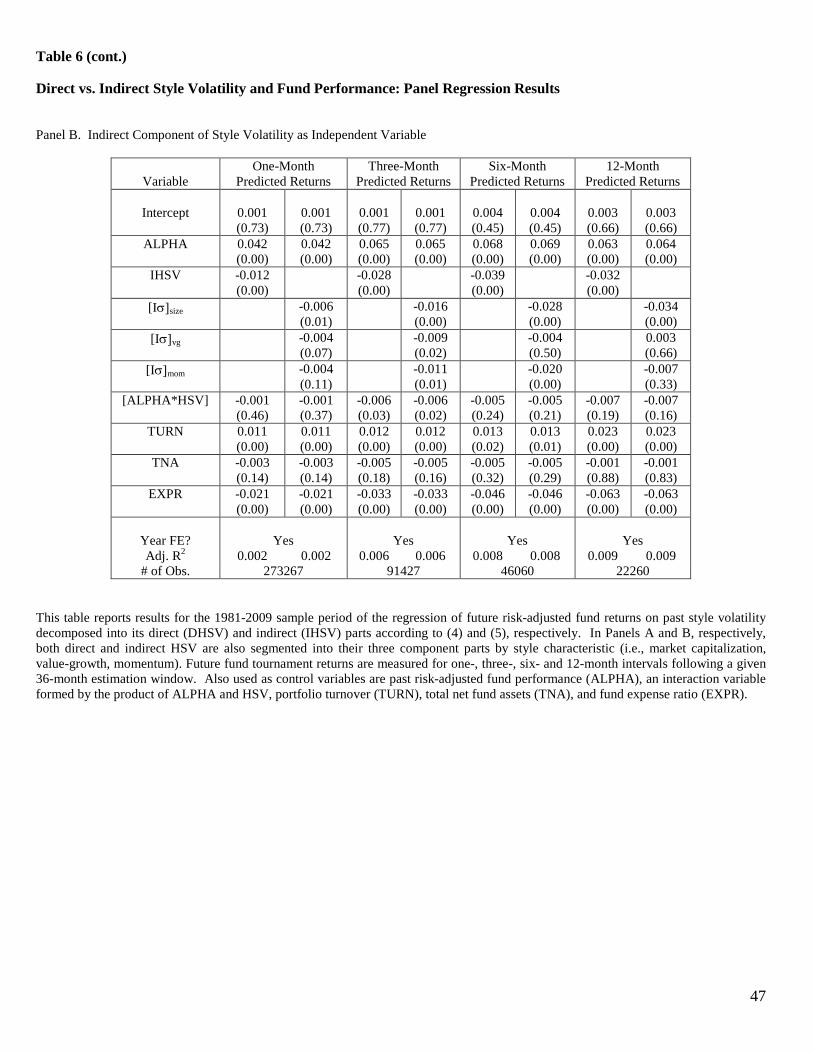
47

Table 6 (cont.) Direct vs. Indirect Style Volatility and Fund Performance: Panel Regression Results

Panel B. Indirect Component of Style Volatility as Independent Variable

Variable

One-Month Predicted Returns

Three-Month Predicted Returns

Six-Month Predicted Returns

12-Month Predicted Returns

Intercept

0.001 (0.73)

0.001 (0.73)

0.001 (0.77)

0.001 (0.77)

0.004 (0.45)

0.004 (0.45)

0.003 (0.66)

0.003 (0.66)

ALPHA 0.042 (0.00)

0.042 (0.00)

0.065 (0.00)

0.065 (0.00)

0.068 (0.00)

0.069 (0.00)

0.063 (0.00)

0.064 (0.00)

IHSV -0.012 (0.00)

-0.028 (0.00)

-0.039 (0.00)

-0.032 (0.00)

[Iσ]size -0.006 (0.01)

-0.016 (0.00)

-0.028 (0.00)

-0.034 (0.00)

[Iσ]vg -0.004 (0.07)

-0.009 (0.02)

-0.004 (0.50)

0.003 (0.66)

[Iσ]mom -0.004 (0.11)

-0.011 (0.01)

-0.020 (0.00)

-0.007 (0.33)

[ALPHA*HSV] -0.001 (0.46)

-0.001 (0.37)

-0.006 (0.03)

-0.006 (0.02)

-0.005 (0.24)

-0.005 (0.21)

-0.007 (0.19)

-0.007 (0.16)

TURN 0.011 (0.00)

0.011 (0.00)

0.012 (0.00)

0.012 (0.00)

0.013 (0.02)

0.013 (0.01)

0.023 (0.00)

0.023 (0.00)

TNA -0.003 (0.14)

-0.003 (0.14)

-0.005 (0.18)

-0.005 (0.16)

-0.005 (0.32)

-0.005 (0.29)

-0.001 (0.88)

-0.001 (0.83)

EXPR -0.021 (0.00)

-0.021 (0.00)

-0.033 (0.00)

-0.033 (0.00)

-0.046 (0.00)

-0.046 (0.00)

-0.063 (0.00)

-0.063 (0.00)

Year FE?

Yes

Yes

Yes

Yes

Adj. R2 0.002 0.002 0.006 0.006 0.008 0.008 0.009 0.009 # of Obs. 273267 91427 46060 22260

This table reports results for the 1981-2009 sample period of the regression of future risk-adjusted fund returns on past style volatility decomposed into its direct (DHSV) and indirect (IHSV) parts according to (4) and (5), respectively. In Panels A and B, respectively, both direct and indirect HSV are also segmented into their three component parts by style characteristic (i.e., market capitalization, value-growth, momentum). Future fund tournament returns are measured for one-, three-, six- and 12-month intervals following a given 36-month estimation window. Also used as control variables are past risk-adjusted fund performance (ALPHA), an interaction variable formed by the product of ALPHA and HSV, portfolio turnover (TURN), total net fund assets (TNA), and fund expense ratio (EXPR).

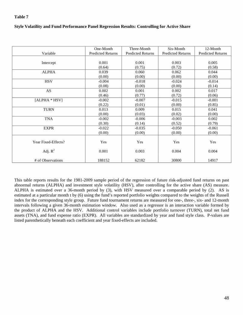
48

Table 7 Style Volatility and Fund Performance Panel Regression Results: Controlling for Active Share

Variable One-Month

Predicted Returns Three-Month

Predicted Returns Six-Month

Predicted Returns 12-Month

Predicted Returns

Intercept

0.001

0.001

0.003

0.005 (0.64) (0.75) (0.72) (0.58)

ALPHA 0.039 0.060 0.062 0.044 (0.00) (0.00) (0.00) (0.00)

HSV -0.004 -0.018 -0.024 -0.014 (0.08) (0.00) (0.00) (0.14)

AS 0.002 0.001 0.002 0.017 (0.46) (0.77) (0.72) (0.06)

[ALPHA * HSV] -0.002 -0.007 -0.015 -0.001 (0.22) (0.01) (0.00) (0.85)

TURN 0.013 0.009 0.015 0.041 (0.00) (0.03) (0.02) (0.00)

TNA -0.002 -0.006 -0.003 0.002 (0.30) (0.14) (0.52) (0.79)

EXPR -0.022 -0.035 -0.050 -0.061 (0.00) (0.00) (0.00) (0.00)

Year Fixed-Effects?

Adj. R2

Yes

0.001

Yes

0.003

Yes

0.004

Yes

0.004

# of Observations

188152

62182

30800

14917

This table reports results for the 1981-2009 sample period of the regression of future risk-adjusted fund returns on past abnormal returns (ALPHA) and investment style volatility (HSV), after controlling for the active share (AS) measure. ALPHA is estimated over a 36-month period by (3), with HSV measured over a comparable period by (2). AS is estimated at a particular month t by (6) using the fund’s reported portfolio weights compared to the weights of the Russell index for the corresponding style group. Future fund tournament returns are measured for one-, three-, six- and 12-month intervals following a given 36-month estimation window. Also used as a regressor is an interaction variable formed by the product of ALPHA and the HSV. Additional control variables include portfolio turnover (TURN), total net fund assets (TNA), and fund expense ratio (EXPR). All variables are standardized by year and fund style class. P-values are listed parenthetically beneath each coefficient and year fixed-effects are included.

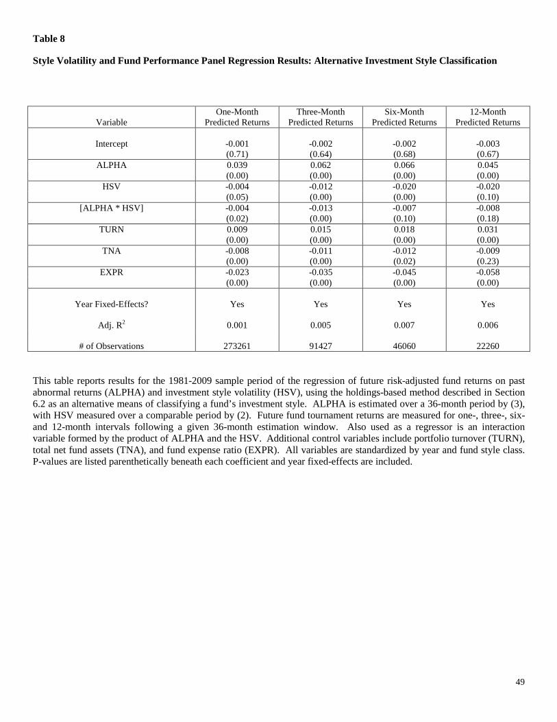
49

Table 8 Style Volatility and Fund Performance Panel Regression Results: Alternative Investment Style Classification

Variable One-Month

Predicted Returns Three-Month

Predicted Returns Six-Month

Predicted Returns 12-Month

Predicted Returns

Intercept

-0.001

-0.002

-0.002

-0.003 (0.71) (0.64) (0.68) (0.67)

ALPHA 0.039 0.062 0.066 0.045 (0.00) (0.00) (0.00) (0.00)

HSV -0.004 -0.012 -0.020 -0.020 (0.05) (0.00) (0.00) (0.10)

[ALPHA * HSV] -0.004 -0.013 -0.007 -0.008 (0.02) (0.00) (0.10) (0.18)

TURN 0.009 0.015 0.018 0.031 (0.00) (0.00) (0.00) (0.00)

TNA -0.008 -0.011 -0.012 -0.009 (0.00) (0.00) (0.02) (0.23)

EXPR -0.023 -0.035 -0.045 -0.058 (0.00) (0.00) (0.00) (0.00)

Year Fixed-Effects?

Adj. R2

Yes

0.001

Yes

0.005

Yes

0.007

Yes

0.006

# of Observations

273261

91427

46060

22260

This table reports results for the 1981-2009 sample period of the regression of future risk-adjusted fund returns on past abnormal returns (ALPHA) and investment style volatility (HSV), using the holdings-based method described in Section 6.2 as an alternative means of classifying a fund’s investment style. ALPHA is estimated over a 36-month period by (3), with HSV measured over a comparable period by (2). Future fund tournament returns are measured for one-, three-, six- and 12-month intervals following a given 36-month estimation window. Also used as a regressor is an interaction variable formed by the product of ALPHA and the HSV. Additional control variables include portfolio turnover (TURN), total net fund assets (TNA), and fund expense ratio (EXPR). All variables are standardized by year and fund style class. P-values are listed parenthetically beneath each coefficient and year fixed-effects are included.

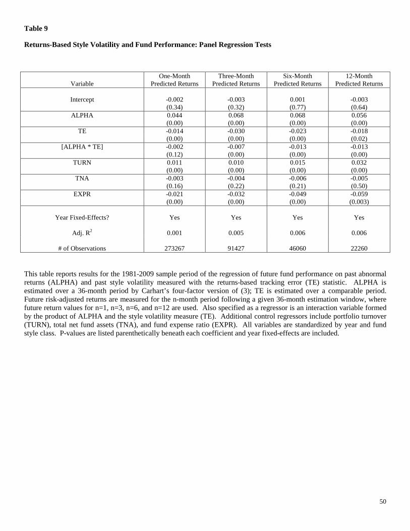
50

Table 9 Returns-Based Style Volatility and Fund Performance: Panel Regression Tests

Variable

One-Month Predicted Returns

Three-Month Predicted Returns

Six-Month Predicted Returns

12-Month Predicted Returns

Intercept

-0.002

-0.003

0.001

-0.003

(0.34) (0.32) (0.77) (0.64) ALPHA 0.044 0.068 0.068 0.056

(0.00) (0.00) (0.00) (0.00) TE -0.014 -0.030 -0.023 -0.018

(0.00) (0.00) (0.00) (0.02) [ALPHA * TE] -0.002 -0.007 -0.013 -0.013

(0.12) (0.00) (0.00) (0.00) TURN 0.011 0.010 0.015 0.032

(0.00) (0.00) (0.00) (0.00) TNA -0.003 -0.004 -0.006 -0.005

(0.16) (0.22) (0.21) (0.50) EXPR -0.021 -0.032 -0.049 -0.059

(0.00) (0.00) (0.00) (0.003)

Year Fixed-Effects?

Adj. R2

Yes

0.001

Yes

0.005

Yes

0.006

Yes

0.006

# of Observations

273267

91427

46060

22260

This table reports results for the 1981-2009 sample period of the regression of future fund performance on past abnormal returns (ALPHA) and past style volatility measured with the returns-based tracking error (TE) statistic. ALPHA is estimated over a 36-month period by Carhart’s four-factor version of (3); TE is estimated over a comparable period. Future risk-adjusted returns are measured for the n-month period following a given 36-month estimation window, where future return values for n=1, n=3, n=6, and n=12 are used. Also specified as a regressor is an interaction variable formed by the product of ALPHA and the style volatility measure (TE). Additional control regressors include portfolio turnover (TURN), total net fund assets (TNA), and fund expense ratio (EXPR). All variables are standardized by year and fund style class. P-values are listed parenthetically beneath each coefficient and year fixed-effects are included.

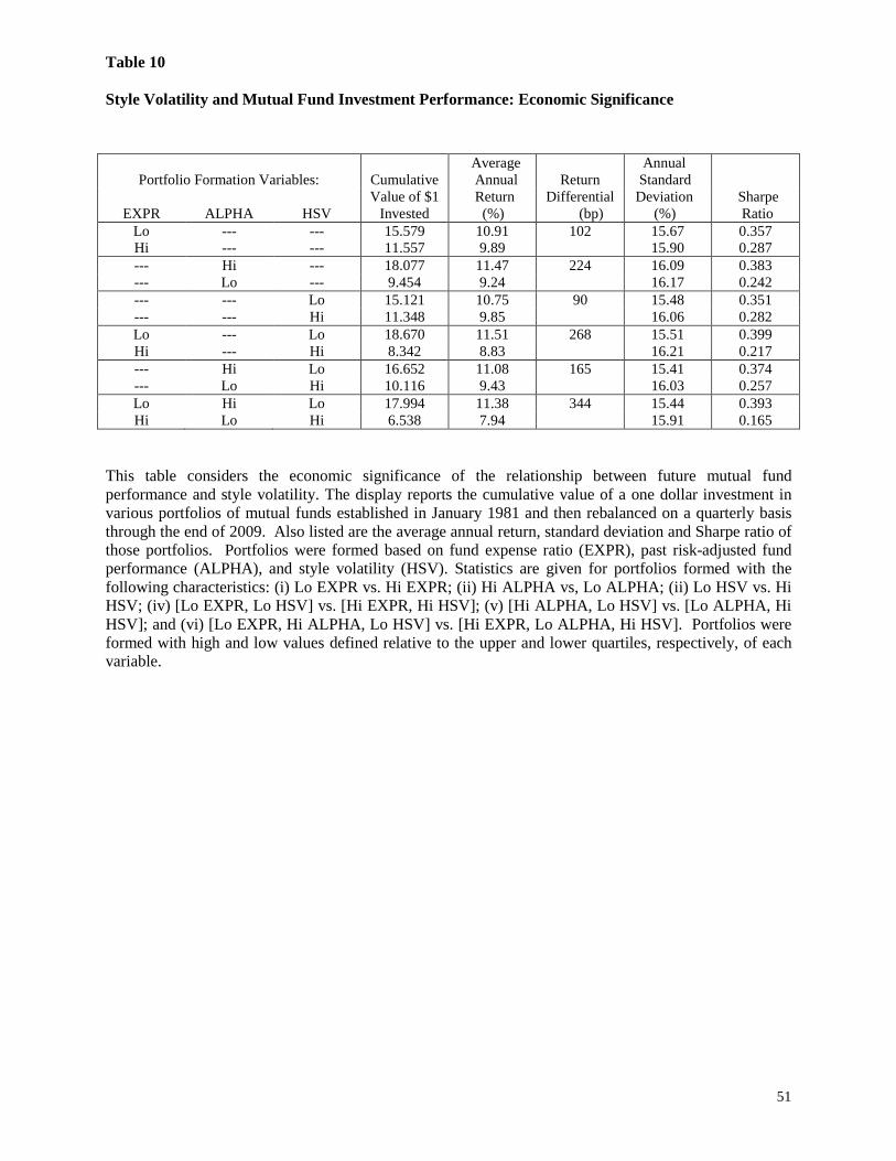
51

Table 10 Style Volatility and Mutual Fund Investment Performance: Economic Significance

Portfolio Formation Variables:

Cumulative Value of $1

Invested

Average Annual Return (%)

Return

Differential (bp)

Annual Standard Deviation (%)

Sharpe Ratio

EXPR

ALPHA

HSV

Lo --- --- 15.579 10.91 102 15.67 0.357 Hi --- --- 11.557 9.89 15.90 0.287 --- Hi --- 18.077 11.47 224 16.09 0.383 --- Lo --- 9.454 9.24 16.17 0.242 --- --- Lo 15.121 10.75 90 15.48 0.351 --- --- Hi 11.348 9.85 16.06 0.282 Lo --- Lo 18.670 11.51 268 15.51 0.399 Hi --- Hi 8.342 8.83 16.21 0.217 --- Hi Lo 16.652 11.08 165 15.41 0.374 --- Lo Hi 10.116 9.43 16.03 0.257 Lo Hi Lo 17.994 11.38 344 15.44 0.393 Hi Lo Hi 6.538 7.94 15.91 0.165

This table considers the economic significance of the relationship between future mutual fund performance and style volatility. The display reports the cumulative value of a one dollar investment in various portfolios of mutual funds established in January 1981 and then rebalanced on a quarterly basis through the end of 2009. Also listed are the average annual return, standard deviation and Sharpe ratio of those portfolios. Portfolios were formed based on fund expense ratio (EXPR), past risk-adjusted fund performance (ALPHA), and style volatility (HSV). Statistics are given for portfolios formed with the following characteristics: (i) Lo EXPR vs. Hi EXPR; (ii) Hi ALPHA vs, Lo ALPHA; (ii) Lo HSV vs. Hi HSV; (iv) [Lo EXPR, Lo HSV] vs. [Hi EXPR, Hi HSV]; (v) [Hi ALPHA, Lo HSV] vs. [Lo ALPHA, Hi HSV]; and (vi) [Lo EXPR, Hi ALPHA, Lo HSV] vs. [Hi EXPR, Lo ALPHA, Hi HSV]. Portfolios were formed with high and low values defined relative to the upper and lower quartiles, respectively, of each variable.

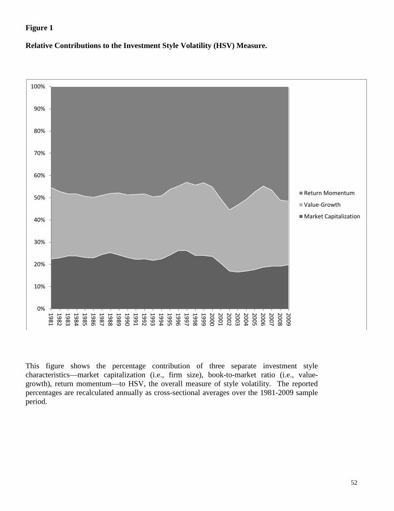
52

Figure 1 Relative Contributions to the Investment Style Volatility (HSV) Measure.

This figure shows the percentage contribution of three separate investment style characteristics—market capitalization (i.e., firm size), book-to-market ratio (i.e., value-growth), return momentum—to HSV, the overall measure of style volatility. The reported percentages are recalculated annually as cross-sectional averages over the 1981-2009 sample period.

0%

10%

20%

30%

40%

50%

60%

70%

80%

90%

100%

19811982198319841985198619871988198919901991199219931994199519961997199819992000200120022003200420052006200720082009

Return Momentum

Value-Growth

Market Capitalization