Embed Size (px)
Citation preview

WORKING PAPER NO. 127
INVESTMENT CLIMATE AND TOTAL FACTOR PRODUCTIVITY INMANUFACTURING: ANALYSIS OF INDIAN STATES
C. VEERAMANIBISHWANATH GOLDAR
April 2004
INDIAN COUNCIL FOR RESEARCH ON INTERNATIONAL ECONOMIC RELATIONSCore-6A, 4th Floor, India Habitat Centre, Lodi Road, New Delhi-110 003
website1: www.icrier.org, website2: www.icrier.res.in

Content
Foreword.................................................. i
Abstract................................................. ii
I Introduction......................................... 1
II Investment Climate in Indian States: Evidence from theExisting Studies..................................... 2
II.1 Labor market regulation......................................................................................................2II.2 Access to Finance ...............................................................................................................4II.3 Land Reform.......................................................................................................................5II.4 Infrastructure ......................................................................................................................5II.5 Business Manager’s Perception of IC in the Indian States .................................................6II.6 Educational Qualification of Manufacturing Workers in the States ...................................7
III Measurement of Productivity.......................... 9
III.1 Multilateral TFP Index .....................................................................................................11
IV Multilateral TFP Estimates for the States: ADescriptive Analysis................................ 12
IV.1 Total Registered Manufacturing Sector ............................................................................12IV.2 TFP at 2-Digit Industry Level: Comparison of Maharashtra, Punjab and Uttar Pradesh..16
V Investment Climate and Total Factor Productivity:Regression Analysis................................. 18
VI Conclusion and Implications......................... 29
References............................................... 31
Appendix-A............................................... 32
Appendix-B............................................... 37

List of Tables
Table 1: Index of Labor regulation in Indian States (cumulative scores for 1992) ........................3
Table 2: Subjective Ranking of Best to Worst IC (FACS 2000) ....................................................6
Table 3: Subjective Ranking of Best to Worst IC (FACS 2003) ....................................................7
Table 4: Percentage of Total Manufacturing Workers (under Regular/Salaried Category) withSecondary Education and Above. .....................................................................................8
Table 5: Multilateral TFP in Registered Manufacturing Sector across Indian States (1980-81to 1999-00)......................................................................................................................13
Table 6: Trend Growth Rates of TFP in Registered Manufacturing Sector (1992-93 to 1999-2000) ...............................................................................................................................15
Table 7: Multilateral TFP across Industries and States.................................................................17
Table 8: Effects of Investment Climate on TFP (Multilateral TFP Index is the DependentVariable, Pooled OLS regression results, 1992-93 to 1997-98) .....................................25
Table 9: Effects of Investment Climate on TFP (Ratio of Real Gross Value Added to Labor isthe Dependent Variable, Pooled OLS regression results, 1992-93 to 1997-98) .............26
Table 10: TFP and Output Lost on account of adverse IC in Various States .................................28
List of Figures
Figure 1 ..........................................................................................................................................9
Figure 2 ........................................................................................................................................14
Figure 3 ........................................................................................................................................14

i
Foreword
ICRIER Working Paper No. 122 identified a slow deterioration in governance asone of the factors in the inability of the economy to show sustained growth take off afterthe reform of the early nineties. This paper investigates some of the elements ofgovernance such as red tape and bureaucracy and the functioning of public utilitymonopolies on economic performance. It does so by first measuring total factorproductivity growth across states and over time and then investigating the impact on TFPGof various governance factors that effect the investment climate. It demonstratesrigorously for the first time how poor governance and investment climate in States has lowproductivity growth and consequently adversely affected overall growth.
We are thankful to World Bank for sponsoring this project. The research washowever carried out independently by ICRIER and any views expressed in the paper arethose of the authors.
(Arvind Virmani)Director & Chief Executive
ICRIERApril 2004

ii
INVESTMENT CLIMATE AND TOTAL FACTOR PRODUCTIVITY INMANUFACTURING: ANALYSIS OF INDIAN STATES
C. Veeramani *Bishwanath Goldar **
Abstract
India has been undertaking significant liberalisation initiatives since 1991 with aview to improving the efficiency of manufacturing industries and achieving faster GDPgrowth. The effects of national level policies can differ considerably across the Indianstates, depending upon the nature of various institutional factors and policies in the states,which can be classified under the broad heading ‘investment climate’ (IC). The presentpaper investigates the influence of IC on the levels of total factor productivity (TFP) in theorganised manufacturing sector across the major Indian states.
Using data from the Annual Survey of Industries (ASI), we estimate multilateralTFP indices for the total registered manufacturing sector in all the major states for theperiod 1980-2000. For a comparison of the states with significantly different IC, we alsopresent detailed estimates of TFP (at the 2-digit industry level) for three states –Maharashtra, Punjab, and Uttar Pradesh. These states are selected on the basis of theobservation that Maharashtra and Uttar Pradesh rank respectively at the top and bottom inthe ranking of states according to IC, while Punjab ranks somewhere in the middle. Thisranking is based on the Firm Analysis and Competitiveness Survey (FACS) conductedjointly by the Confederation of Indian Industries (CII) and the World Bank in 2000 and2003 in the Indian states. A descriptive analysis of TFP in the states’ aggregatemanufacturing and a comparison of TFP in individual industries across the three statesindicate a positive relationship between a market friendly IC and TFP.
For the purpose of this study, the World Bank provided us the tabulated figuresfrom FACS 2003 pertaining to certain quantitative indicators of IC in various industriesacross 12 Indian states. Using these data, we undertook an econometric analysis toinvestigate the influence of various dimensions of IC on TFP of states’ manufacturingindustries during the 1990s. The regression analysis, after controlling for other industryand year specific factors, clearly shows that IC matter for TFP. The dummies for the bestand good IC states yields positive co-efficient with statistical significance, afterconsidering the poor IC states as the base for comparison. Further, as expected, the value
* C Veeramani is Fellow at ICRIER, New Delhi** Bishwanath Goldar is IDBI / IFCI Chair Professor at ICRIER, New Delhi
The authors are grateful to Dr. Arvind Virmani for valuable guidance and encouragement. Commentsfrom Dr. Deepak Mishra of the World Bank were greatly helpful to improve an earlier version of thisreport. Mr. R. Ravishekhar and Mr. Prabhu Prasad Mishra provided competent research assistance for thestudy, which is gratefully acknowledged

iii
of the co-efficient is higher for the best IC states as compared to the good IC states. Thesedummies are based on the subjective notion of IC in the states expressed by businessmanagers. Alternatively, we consider the average number of days required to get a newpower connection in the state as a proxy for IC, which attains a statistically significantnegative co-efficient (the result is the same if the proxy variable used is the number of daysrequired to get a new telephone connection in the state).
The percentage of the management’s time spent with government officials ofregulatory and administrative issues is negatively associated with TFP. Further, mandayslost in industrial disputes has a negative association with TFP. On the other hand, thevariables representing the availability of power for industrial use and disbursement ofcredit in various state industries are found to exert a positive influence on TFP.
In essence, a market friendly IC is essential for achieving higher level of TFP. Thisconclusion is robust, unaffected by the choice of IC indicator. Our analysis also shows thatthere are scopes for initiating policy measures to improve the overall or particulardimensions of IC in almost all the states. States that foster a market friendly IC wouldattract greater investment and grow faster while others lag behind. Thus, it is not surprisingthat India’s overall economic progress since 1991 is leaving some of the states behind.Evidently, the most effective way to eliminate regional growth inequality is to ensure thatthe lagging states initiate reforms to make their IC more market friendly.
Key words: Investment climate, Total factor productivity, manufacturing, Indian states
JEL: L 50, D 24, L 60
1
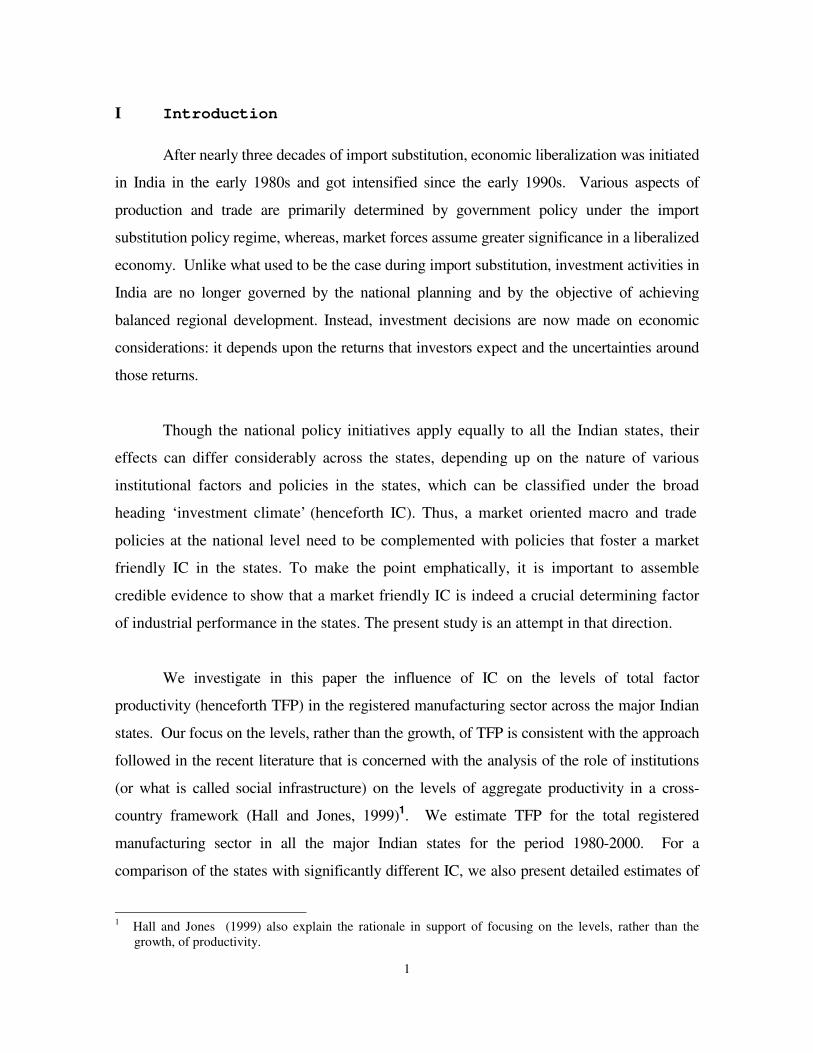
I Introduction
After nearly three decades of import substitution, economic liberalization was initiated
in India in the early 1980s and got intensified since the early 1990s. Various aspects of
production and trade are primarily determined by government policy under the import
substitution policy regime, whereas, market forces assume greater significance in a liberalized
economy. Unlike what used to be the case during import substitution, investment activities in
India are no longer governed by the national planning and by the objective of achieving
balanced regional development. Instead, investment decisions are now made on economic
considerations: it depends upon the returns that investors expect and the uncertainties around
those returns.
Though the national policy initiatives apply equally to all the Indian states, their
effects can differ considerably across the states, depending up on the nature of various
institutional factors and policies in the states, which can be classified under the broad
heading ‘investment climate’ (henceforth IC). Thus, a market oriented macro and trade
policies at the national level need to be complemented with policies that foster a market
friendly IC in the states. To make the point emphatically, it is important to assemble
credible evidence to show that a market friendly IC is indeed a crucial determining factor
of industrial performance in the states. The present study is an attempt in that direction.
We investigate in this paper the influence of IC on the levels of total factor
productivity (henceforth TFP) in the registered manufacturing sector across the major Indian
states. Our focus on the levels, rather than the growth, of TFP is consistent with the approach
followed in the recent literature that is concerned with the analysis of the role of institutions
(or what is called social infrastructure) on the levels of aggregate productivity in a cross-
country framework (Hall and Jones, 1999)1. We estimate TFP for the total registered
manufacturing sector in all the major Indian states for the period 1980-2000. For a
comparison of the states with significantly different IC, we also present detailed estimates of
1 Hall and Jones (1999) also explain the rationale in support of focusing on the levels, rather than the
growth, of productivity.

2
TFP (at the 2-digit industry level) for three states – Maharashtra, Punjab, and Uttar Pradesh.
These states are selected on the basis of the observation that Maharashtra and Uttar Pradesh
rank respectively at the top and bottom in the ranking of states according to IC, while Punjab
ranks somewhere in the middle. This ranking is based on the “Firm Analysis and
Competitiveness Survey (FACS)” conducted across the Indian states jointly by the World
Bank and the Confederation of Indian Industry (CII). The FACS has been conducted twice in
India, one contains data for the year 2000 and the other for the year 2003. The ranking of the
states is on the basis of certain subjective notions of IC expressed by entrepreneurs and
company managers.
The remainder of the paper is structured as follows. In Section II, we provide a brief
overview of the existing studies that deal with the various aspects of IC in the Indian states.
Section III discusses the methodology followed in the present study to measure TFP. A
descriptive analysis of the estimates of TFP in the registered manufacturing sector of the
states for the period 1980-2000 is provided in Section IV. The estimates of TFP for the total
manufacturing are presented for the 17 major states, and at the 2-digit industry level for
Maharashtra, Punjab and Uttar Pradesh. In Section V, we undertake a regression analysis to
investigate the effect of IC on TFP, based on data for the 7 major industries and the 12 major
states covered in FACS 2003. Details about the sources of data and construction of the
variables are explained in the Appendix.
II Investment Climate in Indian States: Evidence from theExisting Studies
In what follows, we provide a brief overview of the studies that deal with the various
aspects of IC in the context of the Indian states.
II.1 Labor market regulation
Labor regulations have been identified as an important element of IC in India. It is
important to note two critical aspects of labor market regulation in India. First, labor
regulation only applies to firms in the registered manufacturing sector. Second, the Indian

3
constitution empowers state governments to amend the Industrial Disputes Act, 1947, which
is the key piece of central legislation that sets out the conciliation, arbitration and adjudication
procedures to be followed in the case of an industrial dispute. The state governments have
extensively amended this Act during the post independence period. Besley and Burgess
(2002) read the text of each amendment over the period of 1958-1992 and coded each
amendment as pro-worker (+1), neutral (0) or pro-employer (-1). This procedure allowed
them to ascertain whether labor regulations in a state are moving in a pro-worker or pro-
employer direction. Having obtained the direction of amendments in any given year, they
cumulated the scores over time to give a quantitative picture of the regulatory environment as
evolved over time.
Following the above procedure, Besley and Burgess (2002) identified four states as
pro-worker. These are: Gujarat, Maharashtra, Orissa and West Bengal. Six states have been
identified as pro-employer: Andhra Pradesh, Karnataka, Kerala, Madhya Pradesh, Rajasthan
and Tamil Nadu. The states that did not experience any amendment over the period are:
Assam, Bihar, Haryana, Jammu and Kashmir, Punjab and Uttar Pradesh. The cumulative
scores for each of the states at the end of the period are shown in Table 1.
Table 1: Index of Labor regulation in Indian States(cumulative scores for 1992)
Pro-WorkerStates
Score Pro-EmployerStates
Score Neutral States Score
West BengalMaharashtraGujaratOrissa
4211
Andhra PradeshTamil NaduKarnatakaKeralaMadhya PradeshRajasthan
-2-2-1-1-1-1
AssamBiharHaryanaJammu and KashmirPunjabUttar Pradesh
000000
Source: Besley and Burgess (2002)
Making use of the variation in labor regulation across states and overtime, for the
period 1958-1992, the regression analysis of Besley and Burgess (2002) indicated
the following.

4
• Moving in a pro-worker direction led to a decline in the per capita output levels
in the registered segment of the manufacturing sector.
• Moving in a pro-worker direction, however, led to an increase in the per capita
output levels in the unregistered segment of the manufacturing sector.
• Moving in a pro-worker direction was associated with increases in urban
poverty but does not affect rural poverty, reflecting the fact that the effects of
labor regulation are mainly being felt in the registered sector which is found
mainly in the urban areas.
Aghion et al (2003), extending the regression analysis of Besley and Burgess
(2002), observed the following:
• States with more pro-worker regulation experienced less growth in output,
employment, labor productivity and TFP for the 1980-1997 period.
• The negative impact of pro-worker regulation got magnified during the post-
liberalization period. Thus, when market access is increased because of
liberalization, it is even more damaging for industries to be located in a pro-
worker state in terms of output, employment, labor productivity and TFP.
II.2 Access to Finance
Access to finance is crucial for the emergence of small business enterprises in rural
areas and hence to reduce rural poverty. Burgess and Pande (2003) analyzed the impacts of
rural branch expansion of banks in India, using panel data of the 16 main Indian states for the
period 1961-2000. The key findings are the following:
• States with more rapid bank branch expansion into unbanked areas experienced
greater increase of per capita output in the unregistered manufacturing sector.
• States with more rapid bank branch expansion into unbanked areas experienced
greater poverty reduction.

5
II.3 Land Reform
State governments in India have jurisdiction over land reform legislation. Besley and
Burgess (2000) exploit this fact to examine whether legislated land reforms had an
appreciable impact on growth and poverty in India. They used panel data on the 16 main
Indian states from 1958 to 1992. By examining and coding the content of each land reform in
a given state, Besley and Burgess (2000) develop a variable that measures the total stock of
land reforms passed in state s by year t. The major finding of the study are:
• After controlling for the effects of other factors, states with greater incidence of
land reforms have done better in reducing poverty.
• Land reform benefited the landless by raising agricultural wages.
II.4 Infrastructure
Mitra et al (2002) examined the effects of infrastructure on TFP and technical
efficiency of the manufacturing industries in the Indian states. They observed marked
disparities in terms of physical, social and economic infrastructure across the states. The
study used annual data from 1976 to 1992 for 17 industries and 15 states. Using the principal
components analysis, a composite indicator of infrastructure availability was developed. The
states that ranked top in terms of infrastructure availability were Maharashtra, Punjab, and
Gujrat, followed by Tamil Nadu, Karnataka and Kerala. States on the lower end of the scale
included Assam, UP, and Bihar, followed by Orissa, Rajasthan and Madhya Pradesh. The
major findings of the study are:
• Infrastructure endowments have a significant role towards explaining the
variation in TFP and technical efficiency across the state industries.
• The key infrastructure related factors for increasing industrial TFP and
technical efficiency are: (i) investment in primary education, (ii) greater
efficiency of the states’ financial system in terms of deposit mobilization and
credit distribution, and (iii) enhancing the potential of power production.

6
II.5 Business Manager’s Perception of IC in the Indian States
The Confederation of Indian Industry (CII) and the World Bank jointly conducted an
Enterprise Survey on 1099 companies across 10 Indian states in the year 2000. The major
industries covered in the study are Textiles, Garments, Pharmaceuticals and Consumer
electronics. The purpose of the survey was to examine the role of IC on the competitiveness
of firms. The business managers were asked to identify the states that they thought had a
better or worse IC than the state in which they were currently based. They were also asked to
say which of the states in their opinion had the best IC and which had the worst. The
subjective ranking of the states according to IC is shown in Table 2.
Table 2: Subjective Ranking of Best to Worst IC (FACS 2000)
States % saying best minus% saying worst
States % saying best minus% saying worst
Best ICMaharashtraGujarat
Good ICTamil NaduKarnatakaAndhra Pradesh
38.6%23.1%
8.6%7.8%6.6%
Medium ICDelhiPunjab
Poor ICKeralaWest BengalUttar Pradesh
1.6%-0.7%
-16.1%-21.9%-32.6%
Source: adapted from CII - World Bank (2002)
The CII-World Bank (2002) study also provides various quantitative indicators across
the 10 states pertaining to (i) the regulatory burden on firms, (ii) the delays at customs houses,
and (iii) the energy and interest costs. Detailed analyses of all these aspects are provided in
the CII-World Bank (2002) study. Here, we highlight only some of the key findings:
• Labor productivity (value added per worker) varies with the IC: the best IC
states have the highest productivity, followed by the good, the medium and the
poor.
• There exists a fairly strong correlation between the subjective judgement of
managers and various quantitative indicators of IC.
• A regression analysis showed that the levels of TFP are lower for the firms
operating in the poor IC states as compared to those in the best, the good and
the medium IC states.
7
• The extent of investment that a state can attract depends crucially upon the IC it
fosters – better governed states attract more investment.
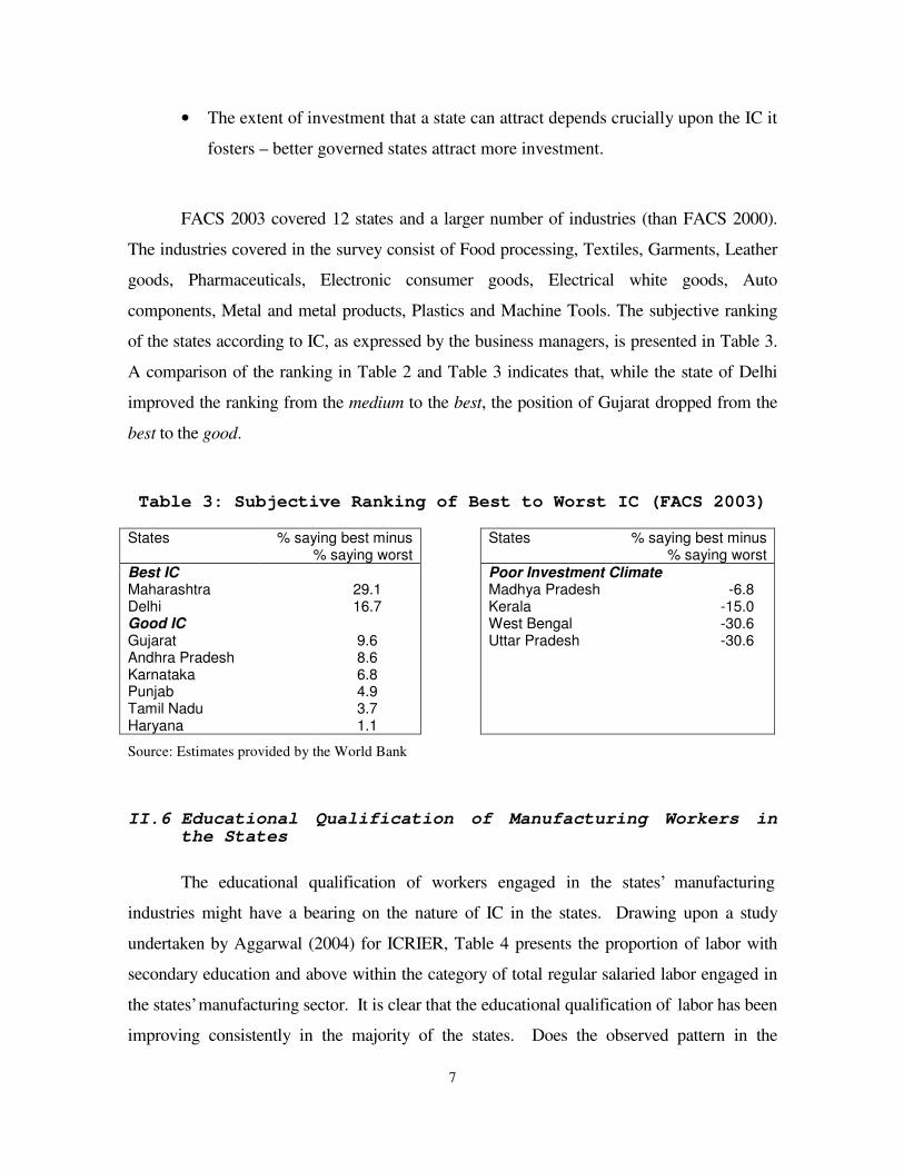
FACS 2003 covered 12 states and a larger number of industries (than FACS 2000).
The industries covered in the survey consist of Food processing, Textiles, Garments, Leather
goods, Pharmaceuticals, Electronic consumer goods, Electrical white goods, Auto
components, Metal and metal products, Plastics and Machine Tools. The subjective ranking
of the states according to IC, as expressed by the business managers, is presented in Table 3.
A comparison of the ranking in Table 2 and Table 3 indicates that, while the state of Delhi
improved the ranking from the medium to the best, the position of Gujarat dropped from the
best to the good.
Table 3: Subjective Ranking of Best to Worst IC (FACS 2003)
States % saying best minus% saying worst
States % saying best minus% saying worst
Best ICMaharashtraDelhiGood ICGujaratAndhra PradeshKarnatakaPunjabTamil NaduHaryana
29.116.7
9.68.66.84.93.71.1
Poor Investment ClimateMadhya PradeshKeralaWest BengalUttar Pradesh
-6.8-15.0-30.6-30.6
Source: Estimates provided by the World Bank
II.6 Educational Qualification of Manufacturing Workers inthe States
The educational qualification of workers engaged in the states’ manufacturing
industries might have a bearing on the nature of IC in the states. Drawing upon a study
undertaken by Aggarwal (2004) for ICRIER, Table 4 presents the proportion of labor with
secondary education and above within the category of total regular salaried labor engaged in
the states’ manufacturing sector. It is clear that the educational qualification of labor has been
improving consistently in the majority of the states. Does the observed pattern in the

8
educational quality of labor indicate a correlation with the perceived IC in the states? Table 4
indicates the answer in the affirmative. States with relatively more educated labor force in the
manufacturing sector are indeed perceived as having better IC (see also Figure 1). The state of
Andhra Pradesh, however, is a clear exception to this pattern.
Table 4: Percentage of Total Manufacturing Workers (underRegular/Salaried Category) with Secondary Education and
Above.
States38th Round ofNSSO (1983)
43rd Round ofNSSO (1987-8)
50th Round ofNSSO (1993-94)
55th Round ofNSSO (1999-00)
Best IC Maharashtra 26.78 31.33 34.79 41.16Delhi 28.24 35.42 39.67 52.62Good ICGujarat 17.75 21.50 30.24 39.39Andhra Pradesh 11.39 13.69 16.91 22.81Karnataka 18.59 17.85 31.70 43.08Punjab 17.36 28.47 32.22 28.12Tamil Nadu 11.67 14.92 20.67 27.56Haryana 18.17 24.76 34.23 37.26Poor ICMadhya Pradesh 10.79 22.32 28.96 31.63Kerala 9.46 12.01 18.16 20.24West Bengal 16.09 15.39 18.50 23.48Uttar Pradesh 10.55 14.25 20.31 23.35Not ClassifiedAssam 11.54 10.23 16.79 16.17Bihar 10.23 21.05 25.26 25.29Himachal Pradesh 17.42 14.06 21.05 34.16Rajasthan 11.50 15.93 19.95 24.00Orissa 8.75 13.59 33.06 20.54II.6.1 All India 15.43 19.18 24.82 29.64
Source: Estimates taken from Aggarwal (2004).

9
Figure 1
R2 is estimated without including Andhra Pradesh. A rank is assigned to the states according to IC on thebasis of Table 3. Accordingly, Maharashtra gets the rank 1. Though Uttar Pradesh and West Bengal sharethe same position according to Table 3, the last rank was assigned to the former on the basis of Table 2.
III Measurement of Productivity
We have used a multilateral TFP index to measure the level of TFP in different states’
manufacturing industries. The multilateral TFP index has the advantage that the productivity
levels can be compared across states and also over time. Productivity level (of manufacturing)
in Maharashtra in 1981-82 is taken as the base and the productivity level in each state-year
(say, Punjab in 1990-91) is compared to this base. Thus, TFP of manufacturing in a particular
state in a particular year is expressed as a ratio to the TFP level of manufacturing in
Maharashtra in 1981-82. Since Maharashatra is the most industrialised state and the one with
the best IC among the Indian states, it was the natural choice as a benchmark. As regard the
choice of 1981-82 as the base year, the reason is that wholesale price indices are available
with base 1981-82, and we have expressed the output and input series at the constant prices of
1981-82.
Educational Qualification of Workers and IC
MH
DL
GJ
AP
KR
PB
TN
HR
MP
KL WB UP
R2 = 0.700
05
101520253035404550
0 1 2 3 4 5 6 7 8 9 10 11 12 13
Ranking of states According to IC
% w
ith s
econ
dary
edu
. and
abo
ve

10
Multilateral TFP estimates have been made for aggregate registered manufacturing
sector in 17 states for the years 1980-81 to 1999-00. Two sets of estimates have been made.
The first set is based on the value-added function. Value added is taken as output, and
physical capital and human capital adjusted labour as the two inputs. The second set is based
on the gross output function, taking gross output as the measure of output, and physical
capital, human capital adjusted labour, materials, energy, and services used as five inputs. As
mentioned above, the output and input series are all expressed at the constant prices of 1981-
82. The procedure adopted for deflation is explained in Appendix-A. It should be pointed out
here that deflators for output, and intermediate inputs used for each state take into account the
industrial composition of the state. For instance, the deflator for manufacturing value added
in a state is constructed as a weighted average of price indices for various two-digit industries,
the weights being based on the relative shares of the 2-digit industries in manufacturing value
added.
Besides estimating TFP of the aggregate registered manufacturing sector in different
states, we have made such estimates for 2-digit industries. These estimates have been made
for 15 major industries for the period 1980-81 to 1999-00 for three states, namely
Maharashtra, Punjab and Uttar Pradesh. Maharashtra and Uttar Pradesh rank respectively at
the top and bottom in the ranking of states according to IC, while Punjab rank somewhere in
the middle. The comparison of TFP of the 2-digit industries across the three states and over
time would be useful for assessing the effect of IC on productivity.
One difference between the TFP estimates for aggregate registered manufacturing and
those for 2-digit industries is that while labour has been adjusted for human capital for the
former, such adjustment could not be made for the latter. Human capital adjusted labour has
been measured as:
SLeH 1.0= ………………………………………………………………….(1)
where H denotes human capital adjusted labour, L is the number of persons engaged
and S is the average years of schooling of the workers engaged in the states’ manufacturing

11
industries (see PREM notes, no. 42, September, 2000, World Bank). Using NSSO survey
data, an estimate of average years of schooling could be made for manufacturing workers in
each state for four years, 1983, 1987-88, 1993-94 and 1999-00.2 These have been
interpolated to work out a series on S for each state for the period 1980-81 to 1999-00.
However, from the NSSO data, it is difficult to make reliable estimates of educational
attainment of workers engaged in various two-digit industries. Therefore, while making the
TFP estimates at 2-digit industry level, adjustment for human capital has not been done.
III.1 Multilateral TFP Index
For the estimates based on the value-added function (taking value added as output,
physical capital and human capital adjusted labor as the two inputs), the multilateral TFP
index may be written as:
cCbb
KHKH cc
bbc
bbc
KHKHY
YTFP
βαβα
=
__
__
...........................................................(2)
Here, the index expresses the productivity level in state-year b as a ratio to the
productivity level in state-year c. Y denotes value added, H human capital adjusted labor and
K physical capital input.
H_ and K
_ are geometric mean of labor and capital across all the observations (state-
years). The exponents α and β are income shares of labor and capital in value added and must
add to one. Let SLb be the income share of labor in state-year b and SL_
the arithmetic mean
of labor share in value added across all the observations. Then, αb may be written as:
2
_
SLbb
SL +=α ……………………………………………………………………...(3)
2 Estimates of the average years of schooling have been made using the detailed data provided by Aggarwal
(2004) on the educational attainment of the manufacturing workers (registered sector) in different states.

12
In a similar way, βb, αc and βc may be defined.
The TFP index for the two-input case given in equation (2) can easily be extended to
cases of more than two inputs. For the index based on gross output function involving five
inputs (human capital adjusted labor, physical capital, materials, energy and services), as
applied here, real value added (Y) is replaced by real gross output (Q). There are other terms
involving comparison of input use in state-years b and c with the sample average (geometric
mean). The exponents are simple averages of the factor shares in a state-year and the average
for all observations, as in equation (3).
IV Multilateral TFP Estimates for the States: A DescriptiveAnalysis
IV.1 Total Registered Manufacturing Sector
Table 5 provides the multilateral TFP estimates for the total registered manufacturing
sector, based on both valued added and output functions, for the 17 major Indian states. It is
clear that the two best IC states recorded the highest TFP levels for all the given time periods.
Also, most of the good IC states show higher TFP levels as compared to the poor IC states. A
striking exception to this pattern is Andhra Pradesh, whose track record with respect to TFP
has been consistently poor. Figure 2 and 3 show the relationship between the subjective
ranking of IC in the states (based on FACS 2003) and the average levels of TFP during the
1990s. It is evident that the states perceived as better with respect to IC were the ones
showing higher TFP levels during the 1990s. As already indicated, a major exception is
Andra Pradesh, which has been perceived as a good IC state, but the performance of that state
in terms of TFP has been consistently poor.

13
Table 5: Multilateral TFP in Registered Manufacturing Sectoracross Indian States (1980-81 to 1999-00)
Based on Value Added Function Based on Gross Output Function
1980-1 to1990-91
1992-3 to1995-6
1996-7 to1999-00
1992-3 to1999-00
1980-1 to1990-91
1992-3 to1995-6
1996-7 to1999-00
1992-3 to1999-00
Best IC
Maharashtra 112.22 126.33 117.23 121.78 106.71 112.15 110.68 111.41Delhi 105.93 132.53 137.96 135.63 103.16 108.58 108.90 108.76
Good ICGujarat 84.88 102.69 90.83 95.91 100.61 108.60 104.74 106.40Andhra Pradesh 64.17 62.82 76.34 69.58 94.96 94.18 99.36 96.77Karnataka 84.66 102.00 92.95 98.12 99.57 105.23 104.01 104.71Punjab 79.06 93.64 108.62 101.13 98.54 104.39 108.73 106.56Tamil Nadu 97.37 102.12 91.36 96.74 103.20 106.78 104.30 105.54Haryana 93.57 100.68 112.26 106.47 101.46 104.00 107.47 105.74
Poor ICMadhya Pradesh 71.13 82.11 88.65 85.38 94.64 99.01 101.51 100.26Kerala 83.13 81.46 97.57 90.67 101.35 100.17 102.71 101.62West Bengal 75.30 73.93 77.03 75.48 97.11 98.27 99.81 99.04Uttar Pradesh 81.73 97.86 94.01 96.21 99.13 105.29 105.41 105.34
Not ClassifiedAssam 98.61 82.05 83.66 82.85 106.24 99.60 100.91 100.26Bihar 62.10 71.85 116.57 91.01 91.95 96.19 108.11 101.30Himachal Pradesh 67.03 90.30 96.14 93.22 93.42 98.31 100.21 99.26Rajasthan 79.26 86.50 85.74 86.12 98.96 104.58 104.63 104.60Orissa 60.85 54.39 60.80 57.60 89.18 88.66 91.79 90.22Note: (1) Averages of TFP levels are shown for four periods. While computing the averages, the years inwhich there was more than 50 per cent increase or decrease in gross output, value added, fixed capital,employment or materials (all real) have been excluded. The purpose is to make the averages less susceptibleto short-terms fluctuations in the data. The same practice is followed in Tables 6 and 7. (2) The year 1991-92has not been considered in the analysis because there was a severe balance of payments crisis in India,affecting the domestic industries.

14
Figure 2
R2 is estimated without including Andhra Pradesh
Figure 3
R2 is estimated without including Andhra Pradesh
INVESTMENT CLIMATE & TFP (OUTPUT FUNCTION)
MAH
DEL
GUJ
AP
KARPUN
TN HAR
MPKER
WB
UP
R2 = 0.608
95
98
101
104
107
110
113
0 1 2 3 4 5 6 7 8 9 10 11 12 13
Ranking of states according to IC
TFP
(AV
199
2-93
to 1
999-
00)
INVESTMENT CLIMATE & TFP (VALUE ADDED FUNCTION)
MAH
DEL
GUJ
AP
KAR PUNTN
HAR
MPKER
W B
UP
R2 = 0.543
50
70
90
110
130
150
0 1 2 3 4 5 6 7 8 9 10 11 12 13
Ranking of states according to IC
TFP
AV
(199
2-93
to 1
999-
00)

15
Table 6: Trend Growth Rates of TFP in RegisteredManufacturing Sector (1992-93 to 1999-2000)
Based on Value Added Function Based on Gross Output FunctionGrowthRate (%p.a.)
Average TFPLevelfrom1992-3 to1994-5
Average TFPLevelfrom1997-8 to1999-00
GrowthRate (%p.a.)
Average TFPLevelfrom1992-3 to1994-5
Average TFPLevelfrom1997-8 to1999-00
Best ICMaharashtra -0.77 124.82 118.50 -0.04 111.32 110.76Delhi 1.69 133.95 141.82 0.25 108.67 109.25Good ICGujarat -2.61 103.64 86.87 -0.78 108.19 103.50Andhra Pradesh 4.68 58.42 76.50 1.18 92.48 99.10Karnataka -2.63 100.82 85.77 -0.35 104.58 101.97Punjab 3.55 94.26 107.90 0.98 104.16 108.68Tamil Nadu -2.36 101.62 89.25 -0.44 106.08 103.58Haryana 3.20 95.17 109.79 0.92 102.34 106.92Poor ICMadhya Pradesh 2.62 76.09 90.97 0.72 97.35 102.10Kerala 3.63 81.46 99.09 0.40 100.17 102.37West Bengal 1.47 73.56 78.45 0.53 97.73 100.20Uttar Pradesh -2.03 99.02 87.50 -0.18 105.08 103.66Not ClassifiedAssam 1.78 80.43 89.84 0.61 98.45 102.19Bihar 9.57 69.54 116.57 2.36 95.18 108.11Himachal Pradesh 1.64 88.99 94.74 0.40 97.53 99.27Rajasthan 0.48 85.40 86.67 0.23 103.97 104.96Orissa 3.71 53.18 65.17 1.02 88.29 93.31
Table 6 presents the trend growth rates of TFP during the 1990s. Comparison of the
growth rates across the states should be made keeping in mind the large differences in the
base period level of TFP in the states. Growth rates are generally found high in states that start
with relatively low levels of TFP at the beginning of the period and vice versa. Thus, states
like Andra Pradesh, Madhya Pradesh, Kerala, West Bengal, Bihar and Orissa, which all had
low TFP levels to start with, showed relatively higher growth rate. Among the best and good
IC states, Delhi, Punjab, Haryana and Andhra Pradesh showed positive productivity growth,
while growth has been negative in other best and good IC states.
Among the poor IC states, Madhya Pradesh, Kerala and West Bengal showed positive
TFP growth. This is not surprising, as the TFP levels at the beginning of the period were
relatively low in these states. Whereas, the state of Uttar Pradesh, which had a TFP level

16
comparable to that of the good IC states at the beginning of the 1990s, showed one of the
lowest TFP levels by the end of the 1990s.
IV.2 TFP at 2-Digit Industry Level: Comparison ofMaharashtra, Punjab and Uttar Pradesh
The analysis in the previous section indicates a positive relationship between TFP in
the aggregate registered manufacturing and a market friendly IC. Does the observed
relationship between IC and TFP hold also at the level of individual industries? We estimate
TFP at the 2-digit level of National Industrial Classification (NIC) for three states with
substantially different IC. The selected states are Maharashtra, Punjab, and Uttar Pradesh.
According to both FACS 2000 and FACS 2003, Maharashtra and Uttar Pradesh ranked
respectively at the top and bottom in the ranking of states according to IC, while Punjab
ranked somewhere in the middle.
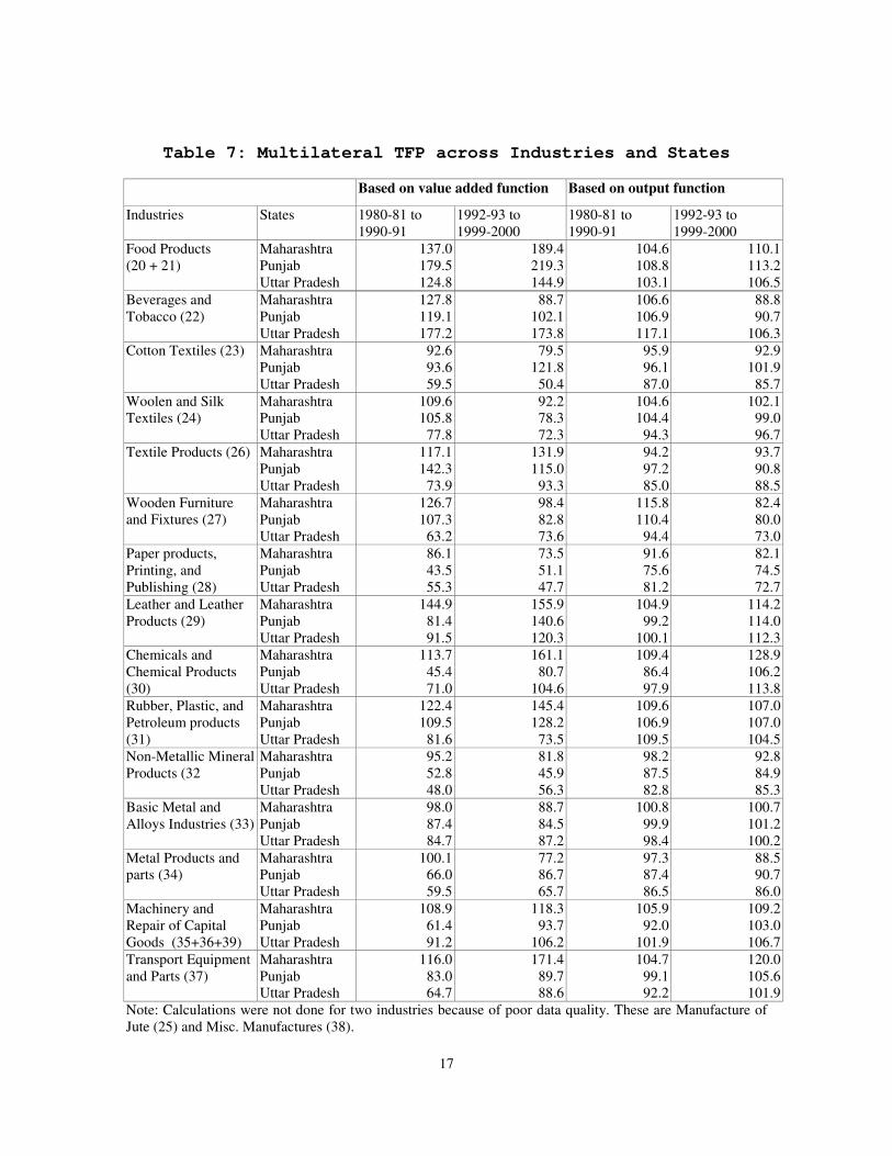
Table 7 shows the 2-digit level estimates of TFP for the three states. The general
pattern is as expected: in most of the industries, Maharashtra shows higher TFP than others,
while Punjab generally achieve higher TFP than Uttar Pradesh. There are, however, certain
important exceptions at the level of specific industries. Punjab shows higher TFP than
Maharashtra in Food Products (during the entire period), Cotton Textiles (during the entire
period), Textile Products (during the 1980s), and Metal Products and parts (during the 1990s).
Beverages and Tobacco is the only industry in which Uttar Pradesh recorded higher TFP as
compared to both Punjab and Maharashtra during the entire period. There is no other single
industry where Uttar Pradesh compares better than Maharashtra, though the former compares
significantly better than Punjab in some cases. These are Paper products, Printing &
Publishing (during the 1980s), Leather and Leather Products (during the 1980s), Chemicals
and Chemical Products (during the entire period), Non-Metallic Mineral Products (during the
1990s), Machinery and Repair of Capital Goods (during the entire period).
In short, the analysis in this section reveal that the observed relationship between IC
and TFP hold also at the level of individual industries. The general nature of IC prevailing in
a state exerts a critical influence for every state industry.
17
Table 7: Multilateral TFP across Industries and States
Based on value added function Based on output function
Industries States 1980-81 to1990-91
1992-93 to1999-2000
1980-81 to1990-91
1992-93 to1999-2000
Maharashtra 137.0 189.4 104.6 110.1Punjab 179.5 219.3 108.8 113.2
Food Products(20 + 21)
Uttar Pradesh 124.8 144.9 103.1 106.5Maharashtra 127.8 88.7 106.6 88.8Punjab 119.1 102.1 106.9 90.7
Beverages andTobacco (22)
Uttar Pradesh 177.2 173.8 117.1 106.3Maharashtra 92.6 79.5 95.9 92.9Punjab 93.6 121.8 96.1 101.9
Cotton Textiles (23)
Uttar Pradesh 59.5 50.4 87.0 85.7Maharashtra 109.6 92.2 104.6 102.1Punjab 105.8 78.3 104.4 99.0
Woolen and SilkTextiles (24)
Uttar Pradesh 77.8 72.3 94.3 96.7Maharashtra 117.1 131.9 94.2 93.7Punjab 142.3 115.0 97.2 90.8
Textile Products (26)
Uttar Pradesh 73.9 93.3 85.0 88.5Maharashtra 126.7 98.4 115.8 82.4Punjab 107.3 82.8 110.4 80.0
Wooden Furnitureand Fixtures (27)
Uttar Pradesh 63.2 73.6 94.4 73.0Maharashtra 86.1 73.5 91.6 82.1Punjab 43.5 51.1 75.6 74.5
Paper products,Printing, andPublishing (28) Uttar Pradesh 55.3 47.7 81.2 72.7
Maharashtra 144.9 155.9 104.9 114.2Punjab 81.4 140.6 99.2 114.0
Leather and LeatherProducts (29)
Uttar Pradesh 91.5 120.3 100.1 112.3Maharashtra 113.7 161.1 109.4 128.9Punjab 45.4 80.7 86.4 106.2
Chemicals andChemical Products(30) Uttar Pradesh 71.0 104.6 97.9 113.8
Maharashtra 122.4 145.4 109.6 107.0Punjab 109.5 128.2 106.9 107.0
Rubber, Plastic, andPetroleum products(31) Uttar Pradesh 81.6 73.5 109.5 104.5
Maharashtra 95.2 81.8 98.2 92.8Punjab 52.8 45.9 87.5 84.9
Non-Metallic MineralProducts (32
Uttar Pradesh 48.0 56.3 82.8 85.3Maharashtra 98.0 88.7 100.8 100.7Punjab 87.4 84.5 99.9 101.2
Basic Metal andAlloys Industries (33)
Uttar Pradesh 84.7 87.2 98.4 100.2Maharashtra 100.1 77.2 97.3 88.5Punjab 66.0 86.7 87.4 90.7
Metal Products andparts (34)
Uttar Pradesh 59.5 65.7 86.5 86.0Maharashtra 108.9 118.3 105.9 109.2Punjab 61.4 93.7 92.0 103.0
Machinery andRepair of CapitalGoods (35+36+39) Uttar Pradesh 91.2 106.2 101.9 106.7
Maharashtra 116.0 171.4 104.7 120.0Punjab 83.0 89.7 99.1 105.6
Transport Equipmentand Parts (37)
Uttar Pradesh 64.7 88.6 92.2 101.9Note: Calculations were not done for two industries because of poor data quality. These are Manufacture ofJute (25) and Misc. Manufactures (38).

18
V Investment Climate and Total Factor Productivity:Regression Analysis
In what follows, we utilize regression technique to investigate whether IC matters for
TFP. The period of the analysis is from 1992-93 to 1997-98. The data at the 2-digit level of
National Industrial Classification (NIC) – 1987 are used for the 12 states covered in FACS
2003. The specific industry groups included in the regression analysis, with the corresponding
two digit codes of NIC, are: (i) Food manufacturing and Processing (20+21); (ii) Textiles
(23+24+25); (iii) Garment (26); (iv) Leather Manufacturing (29); (v) Chemicals (30); (vi)
Machinery (35+36); and (vii) Transport Equipments (37). It may be noted that the selection of
these industries is done keeping in mind the nature of the available data on some of the IC
indicators. Appendix-A discusses the details regarding the nature of the database used in the
regression analysis. Appendix-B gives the average values of the dependent (TFP) and
explanatory variables and inter-correlation matrix among the explanatory variables used for
the regression analysis.
Two alternative econometric approaches are adopted to investigate the effect of IC on
TFP. First, the regression equation specified relates the multilateral TFP index to various
available indicators of IC in the states.
MTFP = γ + δ1 IC1 + δ2 IC2 + ………………+ δn ICn+ u …….(4)
Where MTFP represents the multilateral TFP index (based on the value added
function) in industry (i) state (s) and year (y). For estimating MTFP, the productivity level in
one industry (i.e., Textiles) in Maharashtra in 1981-82 is taken as the base and the
productivity level in each state-industry-year (say, Punjab in Transport Equipments in 1997-
98) is compared to this base. The explanatory variables IC1, IC2, …… ICn are the various
available indicators of IC, and u is the usual error term.
The second approach followed in the present study is similar to that in the CII-World
Bank (2002) study. The regression equation specified relates gross value added-labor ratio to

19
capital-labour ratio, and real wage rate for each industry (i) state (s) and year (y), along with
IC. The relationship is taken to be log-linear in gross value added-labour ratio, capital-labour
ratio and real wage rate. Thus, the regression equation may be expressed as:
ln (Y / L) = α + β1 ln (K / L) + β2 ln (w) + δ1 IC1 + δ2 IC2 + ……+ δn ICn+ u …(5)
where Y is the real gross value added and L is the total labor force engaged in
manufacturing, K is the capital stock, and w is the real wage rate. It may be noted in this
context that in a number of studies, ln (Y/L) has been regressed on ln (K/L) along with other
determinants of productivity. As (K/L) is included as one of the variables to explain (Y/L),
the co-efficients δ1, δ2, …… δn, in effect, captures the effect of IC on TFP rather than labor
productivity. Equation (5) implicitly assumes the underlying production function to be Cobb-
Douglas. By including the real wage rate (w) in the equation, we allow the production
function to be more general. It may be pointed out that a log-linear relationship between Y/L,
K/L and w arises in the Hildebrand-Liu (1965) specification of the Variable Elasticity of
Substitution (VES) production function, which has the Cobb-Douglas, and the CES (Constant
elasticity of substitution) production function as special cases.
To incorporate the effect of IC in the regression model, we consider a number of
alternative variables in equations (4) and (5). In addition, year and industry dummies are
included in all the specifications. This is necessary to control for the influence of year-specific
and various unobserved industry-specific factors.
To begin with, drawing upon the classification of states according to IC in Table 3, we
consider the following indicators:
BestIC Dummy for the best IC states
GoodIC Dummy for the good IC states
The poor IC states are taken as the base for comparison. If IC indeed matters for TFP,
we expect statistically significant positive coefficients for both BestIC and GoodIC. A

20
stronger condition is that the positive coefficient value of BestIC is higher that that of
GoodIC.
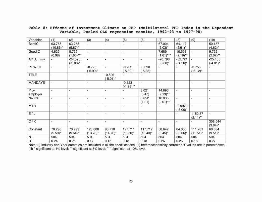
The results of the least square regressions corresponding to equations (4) and (5) are
shown in Table 8 and 9, respectively3. In both the tables, the co-efficient values
corresponding to BestIC and GoodIC are indeed consistent with what is being hypothesized.
The levels of TFP in the best and good IC states are higher than those in the poor IC states.
Furthermore, the best IC states have higher TFP than the good IC states. The values of the t-
ratio and co-efficient corresponding to the variable GoodIC increases significantly when an
additional dummy for the state of Andhra Pradesh is included in equation (4) [compare the
specifications 1 and 2 in Table 8]. Thus, clubbing the state of Andhra Pradesh with the group
of good IC states pulls down the co-efficient value of the variable GoodIC. However, as to
equation 5, the t-value of the co-efficient of GoodIC is very high even without a dummy for
Andhra Pradesh, though including the dummy indeed raises the co-efficient value of GoodIC
[compare specifications 1 and 2 in Table 9]. This result concerning the state of Andhra
Pradesh is expected, as the track record of that state with respect to TFP has been consistently
poor despite being perceived as a good IC state in FACS.
Using similar type of dummy variables as in the present study, the CII-World Bank
(2002) study observed that the group of poor IC states has lower TFP levels as compared to
other states. It is important to note that the dummy variables used in both the studies are
based on the business managers’ perception of IC in various states. The use of such indicator
may well be opposed on the ground that the business managers’ perception could be biased
and may have nothing to do with the actual IC and that the use of some objective indicators of
IC could tell a different story. In addition, some elements of arbitrariness are bound to occur
in the categorization of the states as best, good, and poor IC states. In view of these concerns,
3 Industry and year dummies are included in all the specifications, the base industry taken for comparison
being Textiles while the base year being 1992-93. To economize with space and to simplify the tables,we do not report the co-efficients corresponding to the year and industry dummies. However, it is worthnoting that all the industry and year dummies were positive with statistical significance in most cases.Thus, the levels of TFP are higher in other industries as compared to Textiles and also for other years ascompared to 1992-93. It may also be noted from Table 9 that the underlying production function inequation (5) works well: capital labor ratio (K / L) and real wage rate (w) yield expected signs withstatistical significance.

21
we ask the question: Does the effect of IC on TFP still hold if we use certain quantitative
indicators of IC, instead of the dummy variables? We first consider the following variable.
POWER Average number of days required to get a new power connection in the
state
This variable yields a statistically significant negative co-efficient (see specification 3
in Table 8 and 9) adding credence to the results reported above based upon the dummy
variables. An alternative indicator of IC, which is again quantitative in nature, in the states is:
TELE Average number of days required to get a new telephone connection in the
state
Yet again, the IC variable yields results in the expected line in that the co-efficient of
TELE turns out to be negative and significant in both equation (4) and (5). Thus, the results
obtained with respect to the business managers’ perception of IC are consistent with that
obtained using some of the available quantitative indicators. Clearly, IC matters for TFP,
irrespective of the variables used to measure IC and irrespective of the econometric
approaches followed to analyze the relationship between the two. In what follows, we
consider, one by one, a number of additional quantitative indicators, representing different
dimensions of IC, to further strengthen our conclusion.
Stringent labor regulations have often been identified as one of the major reasons for
the poor competitiveness and growth of India’s manufacturing sector as compared to other
countries. Despite more than a decade of liberalization in various constituents of economic
policies, the policies concerning the labor market continue to be very restrictive in India,
primarily for political reasons4. Nevertheless, states differ to a certain extent with respect to
the degree of labor market flexibility (freedom to hire and fire) and the incidence of industrial
disputes. As already noted, the extent of labor market regulation might vary across the states
4 A number of studies show that labor regulation in India adversely affect not only the competitiveness of
the manufacturing sector but also the overall level of employment, particularly in the registeredmanufacturing sector.

22
as the Indian constitution empowers the state governments to amend the Industrial Disputes
Act, 1947. It is pertinent to examine if the differences in the labour market conditions across
the states have any bearing on TFP in the states’ manufacturing industries. We first consider
the following variable:
MANDAYS Number of man days lost per employee in industrial disputes in state
s and year y
The co-efficient of this variable, as expected, attains negative sign with statistical
significance, suggesting the critical importance of a harmonious industrial relations in the
states. It is difficult to gauge the differences with respect to labour market flexibility
(freedom to hire and fire) across the states. However, we have made use of certain proxy
variables. First, based upon the classification of the Indian states according to labour
regulation by Besely and Burgess (2002) in Table 1, we include the following dummy
variables5:
Pro-employer Dummy for the pro-employer states
Neutral Dummy for the neutral states
The group of pro-worker states is taken as the base for comparison. These variables
are expected to yield positive coefficients with larger value for the former than for the latter.
It is clear from Table 8 and 9 that the co-efficient of both the dummies are indeed positive,
though the value of the coefficient does not turn out to be larger for Pro-employer as
compared to Neutral. Thus, it may be concluded that the states that undertook labor
regulation in the pro-worker direction experienced lower levels of TFP as compared to the
states that undertook regulation in the pro-employer direction or were neutral.
5 The cumulative index of labor regulation (constructed by Besley and Burgess) is available for the year
1992 and before, not for the years considered in our regression analysis. Thus, the dummy variables,rather than the actual cumulative scores for the year 1992, are thought to be appropriate. The state ofDelhi is considered as a neutral state.

23
The tabulated data from FACS 2003, made available to us by the World Bank, include
a variable defined as “excess manpower as percent of total employment”. This variable,
however, did not yield statistically significant negative co-efficient in any of the specifications
and was finally dropped from the analysis.
In short, the above results clearly indicate the adverse effect on TFP of labor unrest in
the states. However, a definite conclusion regarding the effects of labor market flexibility on
TFP does not emerge from our analysis, perhaps because of the inappropriate variables used
to capture labor market flexibility. In this context, however, it is worth referring to the study
by Aghion et al (2003), yet again. Using a larger time series-cross sectional data, they
analyzed the effect of the direction of labor regulation in the Indian states, measured by the
actual Besely and Burgess index, on TFP and other indicators of performance. To reiterate the
findings of Aghion et al (2003), the states with more pro-worker regulation experienced less
growth in labor productivity and TFP (and also other indicators) for the 1980-1997 period and
the negative effect of pro-worker regulation got magnified during the post-liberalization
period. In view of these findings, we tend to believe that labor market flexibility is important
for faster TFP growth, though a definite conclusion does not emerge from the present study.
The extent of the regulatory burden on firm is an indicator of how fair and market
friendly the business environment is. The business environment may be considered more
market friendly if the incidence of regulatory visit to the firm by the government inspectors is
fewer. Thus, we include:
MTR Percentage of the management’s time spent with government officials of
regulatory and administrative issues in industry i and in state s
The coefficient of this variable, as expected, is negative and significant (see Table 8
and 9).

24
A stable and sufficient power supply from the public grid is likely to be crucial for
higher productivity growth. In order to determine the effect of power supply condition in the
state, we include:
E / L Electricity sales (in million KwH) for industrial use as a proportion of
total persons engaged in the state’s registered manufacturing sector in
state s and year y.
This variable yields a statistically significant positive co-efficient suggesting that a
stable and sufficient power supply condition is important for the faster growth of TFP.
Finally, we include the variable:
C / K Real industrial credit by the Scheduled Commercial Banks as a proportion
of capital stock in state s industry i and year y.
As to the effects of industrial credit on TFP, the exact direction of causation appears to
be a matter of some concern. While availability of credit is important for enhancing
productivity, it may also be true that better performing industries and states may get relatively
more credit from the banks as compared to others. To reduce the severity of the simultaneity
problem, one year lagged value of C / K was considered in the regression. The co-efficient of
this variable turns out to be positive and statistically significant (see Table 8 and 9). However,
because of the potential simultaneity problem, the results with respect to industrial credit may
be taken as only suggestive.
25
Table 8: Effects of Investment Climate on TFP (Multilateral TFP Index is the DependentVariable, Pooled OLS regression results, 1992-93 to 1997-98)
Variables (1) (2) (3) (4) (5) (6) (7) (8) (9) (10)BestIC 63.765
(10.86)*63.765(5.87)*
- - - - 67.004(6.03)*
64.117(5.91)*
- 50.157(4.62)*
GoodIC 4.625(0.98)
8.725(1.80)***
- - - - 7.689(1.61)***
10.558(2.19)**
- 9.752(2.02)**
AP dummy - -24.595(-3.88)*
- - - - -26.798(-3.80)*
-32.721(-4.56)*
- -25.485(-4.01)*
POWER - - -0.725(-5.99)*
- -0.702(-5.92)*
-0.690(-5.88)*
- - -0.755(-6.12)*
-
TELE - - - -0.506(-5.01)*
- - - - - -
MANDAYS - - - - -0.823(-1.98)**
- - - - -
Pro-employer
- - - - - 3.021(0.47)
14.895(2.19)**
- - -
Neutral - - - - - 8.652(1.21)
16.835(2.01)**
- - -
MTR - - - - - - - -0.9979(-3.06)*
- -
E / L - - - - - - - - 1150.37(2.11)**
-
C / K - - - - - - - - - 308.544(3.84)*
Constant 70.298(9.59)*
70.299(9.64)*
123.808(13.73)*
98.710(14.76)*
127.711(13.50)*
117.712(13.43)*
58.642(6.45)*
84.056(-3.06)*
111.781(11.51)*
68.834(9.51)*
N 504 504 504 504 504 504 504 504 504 504R2 0.24 0.25 0.17 0.15 0.18 0.18 0.26 0.26 0.18 0.27Note: (i) Industry and Year dummies are included in all the specifications, (ii) heteroscedasticity corrected ‘t’ values are in parentheses,(iii) * significant at 1% level; ** significant at 5% level; *** significant at 10% level.

26
Table 9: Effects of Investment Climate on TFP (Ratio of Real Gross Value Added toLabor is the Dependent Variable, Pooled OLS regression results, 1992-93 to 1997-98)
Variables (1) (2) (3) (4) (5) (6) (7) (8) (9) (10) (11) (12)Ln (K / L) 0.269
(3.83)*0.268(3.82)*
0.290(4.52)*
0.286(4.61)*
0.224(3.03)*
0.256(3.99)*
0.236(3.38)*
0.230(3.38)*
0.222(3.23)*
0.244(3.61)*
0.294(3.94)*
0.251(3.42)*
Ln (w) 0.720(6.54)*
0.696(6.30)*
0.679(8.10)*
0.699(8.68)*
0.781(6.89)*
0.757(8.56)*
0.777(7.12)*
0.779(7.23)*
0.782(7.30)*
0.750(7.02)*
0.729(6.71)*
0.787(7.40)*
BestIC 0.225(3.45)*
0.232(3.54)*
- - 0.147(2.02)**
- 0.207(3.20)*
0.162(2.27)**
0.167(2.37)**
0.212(3.19)*
0.167(2.64)*
0.111(1.64)***
GoodIC 0.150(3.38)*
0.181(4.10)*
- - 0.109(2.45)**
- 0.138(3.25)*
0.122(2.70)*
0.135(3.02)*
0.162(3.80)*
0.155(3.47)*
0.126(2.76)*
AP dummy - -0.205(-3.40)*
- - - - - - - - - -
POWER - - -0.004(-4.84)*
- - -0.003(-4.56)*
- - - - - -
TELE - - - -0.0034(-3.81)*
- - - - - - - -
MANDAYS - - - - -0.011(-2.95)*
- - -0.009(-2.46)*
-0.007(-1.91)**
- - -0.009(-2.49)*
Pro-employer
- - - - - 0.128(3.00)*
0.088(2.09)**
- - - -
Neutral - - - - - 0.178(4.07)*
0.198(4.50)*
- - - -
MTR - - - - - - - -0.008(-2.65)*
-0.008(-2.69)*
-0.009(-2.99)*
- -0.008(-2.46)*
E / L - - - - - - - - 7.260(1.50)
9.957(2.10)**
- -
C / K - - - - - - - - - - 1.222(2.03)**
1.058(1.62)***
Constant 0.123(0.54)
0.068(0.30)
0.373(1.93)**
0.294(1.60)
0.352(1.41)
0.419(2.14)***
0.152(0.68)
0.442(1.74)***
0.341(1.45)
0.192(0.84)
0.143(0.65)
0.455(1.81)***
N 504 504 504 504 504 504 504 504 504 504 504 504R2 0.69 0.69 0.69 0.69 0.69 0.70 0.70 0.70 0.70 0.70 0.69 0.70Note: (i) Industry and Year dummies are included in all the specifications, (ii) heteroscedasticity corrected ‘t’ values are in parentheses,(iii) * significant at 1% level; ** significant at 5% level; *** significant at 10% level.

27
Having established the relationship between a number of IC indicators and TFP, it
now emerges pertinent to provide a rough quantitative assessment of the extent of
productivity and output loss in various states on account of adverse IC. To that effect, we
undertake a simulation exercise utilizing the co-efficient values of some of the important IC
indicators. Our preferred specification to be used in the simulation is specification (7) in
Table 9. This specification of the production function equation (5) yields statistically
significant co-efficient values for Best IC, Good IC, MANDAYS, and MTR, which we utilize
to simulate the extent of TFP and output loss in various states. The two major IC variables
excluded from the simulation (i.e. not included in the chosen specification) are E / L and C /
K, representing electricity sales and industrial credit in the states. The omission of C / K is
deliberate in view of the possible simultaneity problem discussed above. The variable E / L
was dropped on the grounds of statistically insignificance of the coefficient of that variable
when included along with the other variables in the chosen specification, because of potential
multicollinearity.
The FACS 2003 data suggest that the percentage of the management’s time spent with
government officials of regulatory and administrative issues (MTR) is high even in the states
that are otherwise perceived as having the best or good IC in a broader sense. In fact, the
mean value of MTR is found to be the least in two of the poor IC states: Madhya Pradesh and
Uttar Pradesh. Thus, for simulating the TFP and output loss on account of MTR, the state of
Madhya Pradesh, which has the lowest value for MTR, is taken as the norm. As to simulating
the TFP and output loss on account of MANDAYS, the state of Delhi is taken as the norm, as
mandays lost in industrial disputes is the least in that state. As far as the business manager’s
perception of IC is concerned, the best IC states (Maharashtra and Delhi) are taken as the
norm. Under the above assumptions, we simulate the total TFP and output lost in each state
on account of having had failed to attain the best practices with respect to the chosen
dimensions of IC.

28
Table 10: TFP and Output Lost on account of adverse IC inVarious States
MTR MANDAYS(average for 1992-3to 1997-8)
% of TFP lost onaccount of adverse IC
Gross value added (inmillions of rupees) lost in1999-2000 on account ofadverse IC
Best ICMaharashtra 16.17 2.16 -8.70 8381.11Delhi 12.88 0.67 -4.72 4680.97
Good ICGujarat 24.11 2.67 -19.56 13504.05Andhra Pradesh 9.64 5.83 -10.62 11765.05Karnataka 14.77 2.27 -9.05 36834.77Punjab 11.57 2.96 -10.54 4368.75Tamil Nadu 14.23 2.06 -11.02 7421.89Haryana 9.90 4.29 -9.47 7393.146
Poor ICMadhya Pradesh 7.05 0.99 -16.49 5285.17Kerala 21.01 6.76 -32.88 42009.27West Bengal 17.49 19.32 -41.08 74599.32Uttar Pradesh 7.98 2.62 -18.68 47368.27
The results of the simulation are shown in Table 10, which gives a rough idea of the
extent of output lost (in millions of rupees) in one year (1999-2000) across the states. It is
clear that there is scope for improvement in IC in almost all the states. However, the
percentages of output lost are the highest in the poor IC states in general and the states of
West Bengal and Kerala in particular. Within the group of poor IC states, the extent of loss is
less in Uttar Pradesh and Madhya Pradesh as compared to West Bengal and Kerala because of
the relatively better position of the former two states with respect to MTR and MANDAYS.
Among the good IC states, Gujarat suffered the highest on account of the highest incidence of
MTR in that state. The states of Tamil Nadu, Punjab and Karnataka also lost considerably,
particularly on account of high MTR. High incidence of industrial disputes contributed
significantly to the industrial output loss in Andhra Pradesh and Haryana. The states of
Maharashtra and Delhi also experienced output loss on account of regulatory hassles.
In short, the simulation exercise clearly indicates that no single state can be considered
as the best in terms of all the dimensions of IC, though some states, on an average, score

29
better than others. There are scopes for initiating policy measures with a view to improve the
overall or particular dimensions of IC in almost all the states.
VI Conclusion and Implications
The study analyzed the influence of investment climate (IC) on total factor
productivity (TFP) in the registered manufacturing sector across the major Indian states. We
started with a brief overview of the existing studies that deal with the various aspects of IC in
the context of the Indian states. These studies establish the critical importance of labor market
flexibility, access to finance, availability of infrastructure etc for improving industrial
productivity, overall growth, and hence, for eradicating poverty. Appropriate re-distributive
policies such as land reforms also have positive impact on poverty eradication.
The present study provided ample evidence to prove unequivocally that IC matters. A
market friendly IC was found to be essential for achieving higher levels of TFP in the
manufacturing sector. This conclusion is very robust, unaffected by the choice of IC indicator.
New investment will be undertaken only if the IC is market friendly. Under such
circumstances, states that foster better IC would grow faster and be able to eradicate poverty
quicker while others lag behind. Thus, it is not surprising that India’s overall economic
progress during the 1990s has been leaving some of the states behind. Evidently, the most
effective way to eliminate regional growth inequality is to ensure that the lagging states
initiate reforms to make their IC market friendly.
There are scopes for initiating policy measures with a view to improve the overall or
particular dimensions of IC in almost all the states. In particular, the following policy actions
are imperative for enhancing the competitiveness of the manufacturing sector in the states.
• Make the regulatory regime across all the states, including Maharashtra, Delhi and
Gujarat, simpler and hassle free.
• Initiate power reforms to provide a stable and sufficient electricity for industrial use

30
• Introduce legislative changes to make the labor market more flexible, with
appropriate compensation package for labor
• Ensure a harmonious industrial relations in the states
• Improve the availability and quality of basic infrastructure, and
• Provide easy access to finance

31
References
Aggarwal, S.C. (2004) ‘Labour Quality in Indian Manufacturing: A State Level Analysis’,Working Paper (forthcoming), Indian Council for Research on InternationalEconomic Relations, New Delhi.
Aghion, P., Burgess, R., Redding, S., and Zilibotti, F. (2003) ‘The Unequal Effects ofLiberalization: Theory and Evidence from India’:http://econ.lse.ac.uk/staff/rburgess/wp/abrz031002.pdf
Besley, T and Burgess, R (2000) ‘Land Reform, Poverty Reduction, And Growth:Evidence From India’ Quarterly Journal of Economics, Volume 115, 2: 389-430
Besley, T and Burgess, R (2002) ‘Can Labour Regulation Hinder Economic Performance?Evidence from India’ CEPR Discussion Paper No 3260.
Burgess, R and Pande, R (2004) ‘Do Rural Banks Matter? Evidence from the Indian SocialBanking Experiment’ CEPR Discussion Paper No 4211
CII - World Bank (2002), ‘Competitiveness of Indian Manufacturing: Results form a FirmLevel Survey’ Confederation of Indian Industry.
Hall, R, and Jones, C.I., (1999) ‘Why Do Some Countries Produce So Much More Outputper Worker than Others?’ Quarterly Journal of Economics, 114: 83-116.
Hildebrand, G.H. and T.C. Liu (1965), Manufacturing Production Functions in the U.S.,1957: An Inter-Industry and Interstate Comparisons of Productivity, CornellUniversity Press, New York.
Mitra, A., Varoudakis, A., and Véganzonès- Varoudakis, M-A., (2002) ‘Productivity andTechnical Efficiency in Indian States’ Manufacturing: The Role ofInfrastructure’ Economic Development and Cultural Change, 50: 395-426.
Unel, Bulent (2003), ‘Productivity Trends in India’s Manufacturing Sectors in the last TwoDecades’, IMF Working Paper no. WP/03/22.
32
Appendix-A
Database
For making the estimates of TFP, data have been drawn mainly from the Annual
Survey of Industries (ASI), Central Statistical Organization (CSO), Government of India. The
Economic and Political Weekly Research Foundation has created a systematic, electronic
database using the ASI results for the period 1973-74 to 1997-98. Concordance has been
worked out between the industrial classifications used till 1988-89 and that used thereafter
(NIC-1970 and NIC-1987), and comparable series for various three- and two-digit industries
have been prepared. We have used this database for the study, drawing data for the period
1980-81 to 1997-98. For 1998-99 and 1999-00, we have made use of a special tabulation of
the ASI data according to NIC-1987, which was prepared by the CSO for a research project
undertaken at the ICRIER.
For the purpose of deflating output and inputs, wholesale price indices have been used
from the official series on Index number of wholesale prices in India. Construction of
materials and energy price indices requires input-use weights (discussed later), for which the
input-output matrix for 1993-94 prepared by the CSO has been used.
Various IC indicators used in the study come from different sources. For the purpose
of this study, the World Bank provided us the tabulated figures from FACS 2003 pertaining to
some of the IC indicators. These indicators include (i) the subjective ranking of the states
according to IC (see Table 3), (ii) Average number of days required to get a new power
connection in the state (POWER), (iii) Average number of days required to get a new
telephone connection in the state (TELE), and (iv) Percentage of the management’s time spent
with government officials of regulatory and administrative issues in various state industries
(MTR).
Since the IC indicators mentioned above are based on FACS 2003, the selection of the
industries for the regression analysis in Section V was made keeping in mind the major
industries covered in FACS 2003. The industries covered in FACS 2003 are: (i) Food

33
processing, (ii) Textiles, (iii) Garments, (iv) Leather goods, (v) Pharmaceuticals, (vi)
Electronic consumer goods, (vii) Electrical white goods, (viii) Auto components, (ix) Metal
and metal products, (x) Plastics, and (xi) Machine Tools. However, the industry level break-
up of the data on IC indicators, made available to us by the World Bank, exclude the last three
of the above listed industries covered in FACS 2003. Thus, the industry-specific data on
MTR is not available for Metal and metal products, Plastics, and Machine Tools.
Consistent with the nature of FACS data, the industries selected for the regression
analysis, with the corresponding NIC codes, are: (i) Food manufacturing and Processing
(20+21); (ii) Textiles (23+24+25); (iii) Garment (26); (iv) Leather Manufacturing (29); (v)
Chemicals (30); (vi) Machinery (35+36); and (vii) Transport Equipments (37). It is clear that
some of these industries (Chemicals, Machinery and Transport Equipments) do not match
exactly with the industrial break up of FACS 2003, though it is possible to find the exact
mapping for these industries at the 3-digit level of NIC. But this option was not considered
since we noted serious fluctuations in the series at the 3-digit level for the states, possibly
because of significant discrepancies in the ASI with regard to the coverage of and response
from the factories over the years. Data at the 2-digit level industries are used, as the state
level data at that level of aggregation is noted to be free from serious fluctuations. Thus, the
data on MTR corresponding to Pharmaceuticals and Auto components are used respectively
for Chemicals, and Transport Equipments. And, the simple average of MTR in Electronic
consumer goods, Electrical white goods is applied for Machinery.
Data pertaining to electricity sales and credit are from the publications of the Centre
for Monitoring Indian Economy (CMIE), namely “Energy, 2000” and “Money and Banking,
2000”. Credit is deflated by the wholesale price index for machinery. Estimates of mandays
lost per employee in industrial disputes (MANDAYS) are made drawing data from the
“Indian Labor statistics” of the Labor Bureau, Government of India.
34
Measurement of output and inputs
Output: Real gross output and real gross value added are used as the measure of output for
the TFP estimates based on the gross output function and value added function,
respectively. To obtain the output deflator for manufacturing sector in a state, the deflators
constructed for two-digit industries (from the series on wholesale price indices) are
combined according to the relative shares of the 2-digit industries in the manufacturing
output.
Labor: Total number of persons engaged, with adjustments made for human capital based
on average years of schooling, is taken as the measure of labour input. This includes
working proprietors. For TFP estimates at the two-digit level industries, it has not been
possible to make the adjustment for human capital. Therefore, in such estimates, labour
input is measured by the number of persons engaged.
Capital: Net fixed capital at constant prices is taken as the measure of capital input. The
construction of the net fixed capital series has been done by the perpetual inventory
method. The relationship between net fixed capital stock in year T, denoted by KT, the
benchmark capital stock, K0, and the net investment series, {It}, may be written as:
Net investment in year t is related to gross investment in year t and capital stock in the
previous year by the following equation:
Here, GI denotes gross investment and δ is the rate of depreciation, which is taken as five
percent. In this regard, we follow Unel (2003) and assume the average life of fixed assets
to be 20 years.
∑=
+=T
ttT IKK
10
1−−= ttt KGII δ

35
To provide further details of the capital stock measurement, the benchmark (1980-81)
estimate of net fixed capital stock is obtained by applying a factor of 2.57 to the book
value of fixed capital in 1980-81 reported for manufacturing sector in various states in the
ASI, i.e.,
where B0 is the book-value of fixed capital in the benchmark year (1980-81).
The National Accounts Statistics (NAS) provides estimates of net fixed capital stock for
registered manufacturing at current and 1993-94 prices. We take the estimate for 1980-81
and shift the base year of prices to 1981-82 (because all other series used are at the
constant prices of 1981-82). Thus, we obtain net fixed capital stock in registered
manufacturing in 1980-81 at 1981-82 prices. This is divided by the book value of fixed
capital in 1980-81 reported in the ASI. The ratio is found to be 2.57, which has then been
applied for all states.
The method used for the estimation of gross fixed investment at 1981-82 prices is
expressed by the following equation:
In this equation, Bt is the book-value of fixed assets in year t and Dt is the depreciation of
fixed capital in year t as reported in the ASI. Pt is the price index for capital goods (base
1981-82), for which we have used the implicit deflator for gross fixed capital formation for
registered manufacturing in the NAS.
Material input: The reported series on material has been deflated to obtain material input
at constant prices. The construction of the deflator has been done in two steps. In the first
step, a deflator for materials is constructed for each two-digit industry considering the
00 57.2 BK ×=
[ ]t
tttt P
DBBG
+−= −1

36
pattern of materials consumption as given in the input-output table for 1993-94 and taking
wholesale price indices for different input-output sectors (the best available from the
official series are used). In the next step, a weighted average of the materials price index of
different two-digit industries is taken to derive the materials price index for manufacturing
in a state. The weights used are the consumption of material in various two-digit industries
in the state in 1981-82 (based year of price indices).
Energy input: Energy input at constant prices is obtained a manner similar to that used for
materials. For each two-digit industry a price index for energy is formed considering the
relative expenditures on coal, petroleum products and electricity as given in the input-
output table for 1993-94 and using wholesale price indices for these three categories of
products. Then, a weighted average of these indices is taken to obtain an energy price
index for manufacturing in a state. The weights are the expenditure on energy of different
two-digit industries in the state in 1981-82.
Services: ASI does not provide data on services used by industrial enterprises. However,
data are reported on materials, energy (coal, petroleum products, wood, electricity, gas,
etc.) and total inputs. The difference between total inputs and the cost of materials and
energy is taken as a measure of services purchased by the industrial units because a major
part of this likely to be on account of services provided by other agencies. The series so
obtained has been deflated by a deflator for services constructed from the NAS. The input-
output table for 1993-94 indicates the purchases of services (transport, banking and
insurance, etc.) made by the manufacturing sector in that year. For these sectors, the NAS
reports GDP at current and constant prices, which are used to work out implicit deflators.
The input-output table indicates the weights to be used for combining them; these are the
relative size of flows from the services sectors to the manufacturing industries. Thus, a
weighted average of the implicit deflators of different services sectors is taken and a
deflator of services bought by manufacturing industries is formed.

37
Appendix-B
Summary statistics of variables used for regression analysis
Variables Obs Mean Std. Dev.MTFP 504 129.7982 63.5015Y / L 504 0.5132 0.3979K/L 504 1.3521 1.2334w 504 0.1315 0.0684POWER 504 55.9642 22.5964TELE 504 30.5925 23.6491MTR 504 14.4066 7.6016MANDAYS 504 4.3805 5.9038E/L 504 0.0117 0.0044C/K 504 0.0172 0.0382Note: Notation explained in the text.
Inter-Correlation matrix among explanatory variables
K/L w POWER TELE MTR MANDAYS E/L C/KK/L 1.00 - - - - - - -w 0.58 1.00 - - - - - -POWER 0.05 -0.03 1.00 - - - - -TELE 0.07 -0.01 0.59 1.00 - - - -MTR 0.13 0.04 0.10 0.33 1.00 - - -MANDAYS -0.09 0.01 0.14 0.10 0.15 1.00 - -E/L 0.09 0.01 0.14 -0.23 -0.04 -0.35 1.00 -C/K -0.14 -0.05 -0.19 -0.09 -0.02 -0.05 -0.05 1.00Pro- Employer -0.13 -0.12 0.29 0.18 -0.10 -0.22 0.02 0.18Neutral 0.07 -0.04 -0.38 -0.15 -0.32 -0.21 -0.02 0.20Pro-Worker 0.01 0.18 -0.16 -0.17 0.43 0.36 0.07 -0.04BestIC -0.01 0.23 -0.31 -0.27 0.01 -0.23 0.11 0.45GoodIC -0.01 -0.19 -0.02 -0.12 0.02 -0.18 -0.09 -0.23PoorIC 0.02 0.03 0.26 0.34 -0.03 0.37 0.01 -0.11


![QUANTIFYING TRADE BARRIERS: HAS PROTECTION …(1989), Aksoy (1991), Aksoy and Ettori (1992), Goldar and Hasheem (1992), Gang and Pandey (1998) and Hasheem (2001)]. Despite attempts](https://img.pdfslide.us/doc/110x75/60cce21654b68112cb4c0bdb/quantifying-trade-barriers-has-protection-1989-aksoy-1991-aksoy-and-ettori.jpg)