Embed Size (px)
Citation preview
Investing into Bargaining Power
Sarah Auster Nenad Kos Salvatore Piccolo ∗
November 17, 2017
Abstract
We study a model of surplus division with costly investments in a bilateral trade
environment. Investments determine the probability with which agents get to make
an offer and thereby the surplus they are able to secure, however, it may also signal
their private information, something that the rival can use to his advantage. We
characterize the equilibria of the game and show that the seller’s payoff can be
non-monotonic in the share of high value buyers. The seller faced with an entry
decision might, therefore, find it propitious to enter a market mostly populated by
low value costumers. JEL Code: C72, D82, D83
Keywords: Bilateral Trade, Bargaining Power, Contests
∗Auster: Bocconi University, Department of Decision Sciences and IGIER. E-mail:[email protected]. Kos: Bocconi University, Department of Economics and IGIER. E-mail: [email protected], Piccolo: University of Bergamo, E-mail: [email protected] would like to thank Alp Atakan, Mehmet Ekmekci, Dino Gerardi, Toomas Hinnosaar, JohannesHorner, Ole Jann, Markus Reisinger, Thomas Wiseman and seminar audiences at Frankfurt School ofManagement, Essex, 2016 CSEF-IGIER symposium, Workshop on Economic Theory, Graz 2016, andWorkshop on Advances in Industrial Organization, Bergamo 2017. This paper was previously circulatedunder the title Competing for surplus in a trade environment.
1
Contents
1 Introduction 1
2 The Baseline Model 5
2.1 Optimal Bargaining Effort . . . . . . . . . . . . . . . . . . . . . . . . . . 6
2.2 Comparative Statics . . . . . . . . . . . . . . . . . . . . . . . . . . . . . 12
3 Two-Sided Effort 14
3.1 Equilibrium Analysis . . . . . . . . . . . . . . . . . . . . . . . . . . . . . 15
3.2 Comparative Statics . . . . . . . . . . . . . . . . . . . . . . . . . . . . . 19
4 Discussion 20
4.1 Effort Costs and Welfare . . . . . . . . . . . . . . . . . . . . . . . . . . . 20
4.2 Probabilistic Bargaining Model . . . . . . . . . . . . . . . . . . . . . . . 22
5 Concluding Remarks 24
6 Appendix 25
1 Introduction
Situations in which agents exert effort or make investments to improve their bargaining
position are ubiquitous: potential buyers search the internet for information on how to
bargain with car salesmen, companies and individuals hire lawyers or other experts when
selling or buying valuable assets, parties in a troubled marriage find divorce lawyers to
negotiate on their behalf, just to name a few.
The amount of resources people invest in improving their bargaining position depends
not only on their individual characteristics, such as their innate ability to negotiate and
the value attached to the deal they bargain over, but also on the rival’s expected strength,
and the possible information that these actions may signal. Highlighting the forces that
shape these investments and the underlying trade-offs is an important step towards a
better understanding of how people bargain and why they choose to do so in certain
environments (markets).
We address these issues by studying a model in which parties can exert costly effort
in order to improve their bargaining position—e.g., the amount of resources spent to
find and hire the right lawyer (or other representatives) negotiating on their behalf, the
amount of attention and time they devote to specialized courses on ‘the art of negotiation’
(see Cialdini and Garde (1987), Fisher et al. (2011)), etc. We consider a stylized bilateral
trading problem between a seller (she) and a buyer (he) who is privately informed about
his valuation. The seller’s value is commonly known and normalised to zero, the buyer’s
value is either low or high, but always above the seller’s. The agents choose between
exerting or not exerting effort. Effort comes at a cost and determines the probability
with which either party gets to make an offer through a success function. Naturally,
exerting effort increases the agent’s chance of proposing a price. The opponent accepts
or rejects the proposal and the game ends.
We do not claim that this is precisely how bargaining unfolds. Rather, our environment
should be interpreted as a reduced form model capturing two salient features. First, if
agents invest effort, they are able to obtain a higher share of surplus. This is captured
through an increase in the probability that they win the opportunity to make an offer.
Second, agents learn about their opponents during the bargaining process. Specifically, if
a certain type of buyer exerts less effort compared to others, then the seller is more likely
to secure the chance to make an offer against that type. The revelation that the seller is
the one who gets to make an offer can, therefore, be a signal of the buyer’s willingness
to pay. Our objective is to analyze how these two elements interplay, and what novel
insights their interaction delivers.
We first consider a simplified version of the model in which the seller’s effort is fixed;
the seller’s only choice is which price to offer. Whenever the buyer gets to make an offer,
he optimally offers price zero. On the other hand, if the seller is to make an offer, she
chooses between a low price that both types of the buyer accept and a high price that
is accepted only by the high value buyer. Whether the low or the high price is optimal
depends on the seller’s posterior belief—the probability that she attaches to the buyer
being the high type—, which is determined by the equilibrium effort decision of the buyer.
The analysis proceeds by observing that the high valuation buyer always has at least as
high an incentive to exert effort as the low valuation buyer—a monotonicity results. The
difference in incentives is strict only if the buyer expects the seller to offer the high price
with strictly positive probability. When the high type exerts effort more often than the
low type, the seller is more likely to secure the opportunity to make an offer against the
low type, thus, the right to make an offer depresses the seller’s belief. As a consequence,
conditionally on making an offer, the seller’s posterior is never above her prior.1
Of interest is the domain where the buyer’s cost of effort is not too extreme. The low
type buyer optimally refrains from effort, while the high type’s effort choice depends on
the seller’s behavior. The analysis is split according to the seller’s prior. When the seller’s
prior is low he offers the low price, neither type exerts effort, and consequently, the seller
learns nothing. The most interesting case arises for intermediate values of the prior. In
this region, if the seller were to naively follow the prior she would offer the high price.
This would incentivize the high type buyer to exert effort and the seller’s posterior would
fall. Subsequently the seller would prefer to offer the low price. The seller offering the
low price, on the other hand, would make the high type buyer best respond by refraining
from effort. The seller’s posterior then would coincide with the prior, and the seller would
in fact best respond with the high price. To escape such cycling of beliefs, the two players
need to randomize: the high type buyer randomizes over the effort choices in such a way
that the seller is indifferent between the two prices, the seller in response randomizes
over the two prices in order to render the high type buyer indifferent between the two
effort choices. Finally, for high priors, the seller offers the high price and the high type
buyer exerts effort. The seller learns and revises her belief downward, but the prior is
sufficiently high so that even after the belief revision the high price is preferable.
We then explore how the seller’s payoff varies with the proportion of the high types.
Our main finding shows that the seller’s payoff is non-monotonic: it is constant in the
fraction of high types for low priors, decreasing for intermediate priors and increasing
for high priors. The striking feature that a higher proportion of high value buyers can
1On the other hand, when the buyer gets to make an offer, the seller’s posterior is weakly greaterthan her prior. Due to the private value assumption, however, the seller’s posterior belief in this case isirrelevant.
2

be detrimental to the seller’s payoff arises as a consequence of the strategic interaction.
In the intermediate region of priors, where buyer and seller use a mixed strategy, the
probability with which the high type buyer exerts effort increases in the seller’s prior: as
the prior increases, the high type buyer has to separate himself further from the low type
in order to keep the seller’s posterior constant. The seller, therefore, gets to make an
offer less often. At the same time, the seller is indifferent between the two prices, so her
payoff conditionally on making an offer does not change with the prior. As a result, her
total payoff is declining. The result has interesting consequences for entry games. If the
seller could choose to enter one of two markets, she might indeed enter a market with a
larger proportion of the low value buyers. Although the buyers with low valuations offer
less surplus to be shared, they also put up less of a fight when splitting the said surplus.
In the richer version of the model the seller can also choose to exert effort. The seller’s
effort has two effects. First, the effort influences the probability that the seller gets to
make an offer. Second, it affects the seller’s learning. We show that the seller learns less
when she exerts effort, or with other words, when exerting effort her posterior declines to
a smaller extent. Several results are qualitatively similar to the environment where the
seller does not exert effort, however a novel behavior arises in a region of parameters: the
seller randomizes over pairs of efforts and prices—no effort coupled with the low price
and effort coupled with the high price. Such mixing is a consequence of the fact that
the seller’s posterior is higher when she exerts effort than when she does not. Intuitively,
when the seller does not exert effort, having the right to make an offer suggests to a
higher degree that the buyer has not exerted effort himself and is therefore more likely
to have a low valuation.
We also explore the welfare effects of bargaining and, in particular, discuss the role of
the buyer’s and seller’s effort costs. In equilibrium each party’s probability of exerting
effort decreases in their own effort cost, as one might expect. Effort cost then affects
welfare through three channels. First, it directly affects the size of the loss incurred in
equilibrium through the cost of effort. Second, it changes the relative probability of the
informed and uninformed party making an offer. Whenever the buyer makes an offer,
trade happens with probability one, whereas if the seller makes an offer, trade may fail.
Third, effort has an effect on how much the seller learns in equilibrium. After exerting
effort the seller is more likely to be inclined to offer the high price which can result in
trade breaking down.
Our results have bearing on the so called probabilistic bargaining models. In such
models the buyer and the seller have exogenously fixed probabilities of making an offer.
Moreover, these probabilities tend to be interpreted as bargaining powers; see for example
3
Merlo and Wilson (1995), Okada (1996), Zingales (1995), Inderst (2001), Krasteva and
Yildirim (2012) and Munster and Reisinger (2015). Our findings imply that in some envi-
ronments it would be more realistic to assume that bargaining power is increasing in the
buyer’s valuation.2 We show that taking the probability of making an offer exogenously
increasing in the buyer’s type provides the researcher with a simpler model than ours,
yet captures some of its arresting features.
Related Literature: The foundation for models of non-cooperative surplus division
under complete information was set by Stahl (1972) and Rubinstein (1982). Stahl (1972)
proposed a finite time model in which two agents alternate in proposing a division of a
commonly known surplus until an offer is accepted, Rubinstein (1982) solves for the infi-
nite horizon version of the game. Our model is closer in spirit to incomplete information
bargaining models as in Fudenberg and Tirole (1983) and Gul, Sonnenschein, and Wilson
(1986). It shares with the dynamic models the feature that the seller’s belief declines
after some information is revealed, however, the structure of the equilibria and the shape
of equilibrium payoffs—the non-monotonicity of the seller’s payoff—are specific to our
work.3
Most related to our paper are models by Evans (1997), Yildirim (2007), Yildirim (2010)
and Board and Zwiebel (2012). Evans (1997) studies a model of coalitional bargaining in
which agents exert effort to win the right to propose and shows that the set of equilibria
coincides with the core. Yildirim (2007) and Yildirim (2010) study a sequential bargaining
model in which agents exert efforts to be the proposer of a split of a pie of a fixed
and commonly known size. After the proposer is chosen and the proposal is made, the
agents vote on whether to accept it. The focus is on how different voting rules affect
the bargaining outcome. Board and Zwiebel (2012) study a similar model with two
agents who repeatedly compete to make an offer to each other for a fixed pie until one
of the offers is accepted. The competition is in the form of a first price auction, and the
agents are endowed with a limited bidding capital. They characterize how the bargaining
outcomes depend on the size and distribution of the bidding capital. Unlike our model,
these papers analyse environments where the surplus is of commonly known size.
Finally, Heinsalu (2017) studies a market with adverse selection, where a seller, pri-
vately informed about the quality of his good, invests into access to a market. The key
differences to our framework are the assumptions that values are interdependent and that
the uninformed party has no bargaining power.
2Grennan (2014) provides evidence that heterogeneity of bargaining power across agents plays animportant role in the market for medical devices.
3In the two period model of Fudenberg and Tirole (1983) the seller makes all the offers. The sellernever randomizes on equilibrium path, while the high type buyer randomizes over his decisions only inthe highest region of priors.
4
2 The Baseline Model
A seller and a buyer want to trade an object. The seller’s valuation is commonly known
and normalised to zero, while the buyer’s valuation v is either high or low, denoted by
vH and vL respectively. We assume vH > vL > 0 and denote the probability that the
buyer’s valuation is vH by µ. After learning his type, the buyer decides whether to exert
effort; his effort choice is denoted by eb ∈ {0, 1}. Effort affects the buyer’s probability
of making an offer to the seller. Let kbeb denote the cost of effort and let ρ1 (resp. ρ0)
denote the buyer’s probability of making an offer to the seller when he does (resp. does
not) exert effort. We assume 0 < ρ0 < ρ1 < 1. The seller gets to make an offer with the
remaining probability. After the offer is accepted/rejected the game ends.
In the baseline model we keep the seller’s effort fixed. The seller potentially learns
about the buyer’s type through the possibility of making an offer and moreover the extent
to which the seller learns may depend on her choice of effort. Shutting down the seller’s
effort component enables us to distill the direct effect of learning on the equilibrium
outcome. Later we relax this assumption in order to see how the effects of the seller’s
effort interplay with learning.
A pure strategy for the buyer is a tuple (eb, pb) for each type, where pb ∈ R denotes the
price the buyer proposes when called upon. The seller only chooses a price offer ps ∈ R.
Remark 1. An example to keep in mind is that of a Tullock contest in which agents’
chances to make an offer are commensurate to their effort investments. More precisely,
suppose that the buyer can choose between two actions {eL, eH}, where eH > eL > 0,
and the seller’s action is fixed to es. The probability that agent i gets to make an offer isei
ei+ej, where ej is the opponents effort. The buyer incurs cost kb(eb − eL) from exerting
effort eb, while the seller incurs no cost. Our model corresponds to setting ρ1 , eH
eH+es
and ρ0 , eL
eL+es.
We call a profile of strategies and a belief function an equilibrium if the strategies are
sequentially rational given the beliefs and the beliefs are updated using Bayes rule when-
ever possible. In addition, we assume that each agent after their own deviation presumes
that the other agent has followed his equilibrium strategy. Two types of off-equilibrium
paths are possible. First, an agent could be the one making an offer after an own de-
viation in effort. In such a case, he computes the posterior using his deviation strategy
and equilibrium prescribed strategies for the opponent. Second, an out of equilibrium
price could be announced. The beliefs at such a node, however, are irrelevant due to the
private values structure of the model.
5
We maintain two interpretations for the effort decision in this environment. First,
agents often exert effort during or prior to the bargaining. They read a book that (pre-
sumably) increases their bargaining skills, e.g. Cialdini and Garde (1987), Trump and
Schwartz (2009), they attend a course on bargaining, or they search the internet for
advice. Data shows, for instance, that people spend on average more than eight hours re-
searching how to bargain before they buy a car in the US.4 Second, agents find specialists
to negotiate on their behalf, especially when an asset has significant value. These spe-
cialists can take the form of lawyers and/or negotiation consultants. Marital dissolution,
for example, is a multibillion dollar business.5
The outlined model, as always, is a simplified representation of reality. We do not
claim that bargaining proceeds precisely as specified above. However, the model does
capture two important features that we would like to explore: 1.) A larger investment
in bargaining enables the agent to secure a higher share of the surplus. This is captured
by the probability with which an agent gets to make an offer. In fact, the existing
literature commonly uses the probability that an agent makes a take-it-or-leave-it offer
as a proxy for bargaining power (see for example Zingales (1995) and Inderst (2001) ).
2.) By observing the opponent’s bargaining stance, an agent may learn something about
the opponent’s type. The seller faced with an opportunity to make an offer can infer
something about the buyer’s valuation due to different types of buyer making (possibly)
different effort decisions.
2.1 Optimal Bargaining Effort
It is useful to start with some preliminary observations. If the buyer gets to make an
offer, he optimally offers price pb = 0. The buyer’s strategy can therefore be reduced to
the probability with which he exerts effort. Let this probability be denoted by βi when
the buyer’s type is i = L,H. On the other hand, if the seller gets to make an offer she
either offers the pooling price vL or the separating price vH . The seller’s strategies can
thus be reduced to the probability with which she offers price vH ; denoted by σ ∈ [0, 1].
The buyer type vi’s expected payoff from exerting effort eb ∈ {0, 1} when the seller
uses the strategy σ is
ρebvi + (1− ρeb)Eσ[1[ps≤vi](vi − ps)]− kbeb,
where Eσ is the expectation operator with respect to the seller’s strategy. After making
4See http://agameautotrader.com/agame/pdf/2016-car-buyer-journey.pdf5 See http://www.huffingtonpost.com/susan-pease-gadoua/divorce-is-big-business-a b 792271.html
6
an effort choice eb the buyer gets to make an offer with probability ρeb and obtains a
payoff equal to vi. With the complementary probability the seller makes an offer, which
the buyer accepts as long as his valuation is not below the price.
Of particular interest will be the buyer’s benefit from exerting effort (rather than not
exerting it), which can be written as
∆ub(vi) = ∆ρ︸︷︷︸,ρ1−ρ0
(vi − Eσ[1[ps≤vi](vi − p)]
)− kb. (1)
The term ∆ρ measures the increase in the probability of the buyer making an offer due to
exerting effort, while the second factor is the increase in the buyer’s payoff when he makes
the offer instead of the seller. If the buyer proposes the price, his payoff is vi, whereas if
the seller makes an offer, the buyer’s payoff is vi − p if he accepts and 0 otherwise.
An important consequence of the above derived benefits is that the high type buyer’s
incentives to exert effort are at least as high as those of the low type.
Lemma 1. For any strategy σ, we have ∆ub(vH) ≥ ∆ub(vL), where the inequality holds
with equality if and only if Eσ[ps] = vL.
The above result follows after a closer inspection of the buyer’s benefits from exerting
effort. For the low type buyer expression (1) simplifies to
∆ub(vL) = ∆ρ vL − kb. (2)
The increase in the buyer’s payoff when making an offer is vL; if the seller gets to make
an offer, the low type buyer’s payoff is zero as he either rejects the seller’s offer or pays
a price equal to his valuation. The low type buyer, therefore, benefits from expending
effort if and only if kb ≤ ∆ρ vL. As a result, the low type buyer’s optimal strategy is
independent of the price the seller charges. If his cost kb is sufficiently small he exerts
effort, otherwise he does not.
The high type buyer’s benefits from switching to exerting effort is
∆ub(vH) = ∆ρEσ[ps]− kb. (3)
The high type always accepts the seller’s offer, so his gain from making the offer himself
is the price he does not have to pay. The higher he expects this price to be, the larger are
his benefits. Given that the expected price the seller charges, Eσ[ps], is weakly greater
than the valuation of the low type buyer, Lemma 1 follows. Moreover, when Eσ[ps] is
7
equal to vL, that is, when the seller offers the low price with certainty, the incentives to
exert effort are the same for both types of buyer.
As to the high type, since Eσ[ps] belongs to the interval [vL, vH ], we have
∆ρ vL − kb ≤ ∆ub(vH) ≤ ∆ρ vH − kb.
The high type buyer thus has two dominance regions: he always exerts effort when the
cost of effort is sufficiently small; in particular kb < ∆ρ vL. In that case, the buyer finds it
worth to expend effort even if he expects the seller to charge price vL. On the other hand,
when the cost of effort is so high that even if the seller charges the high price exerting
effort is not optimal, i.e. ∆ρ vH < kb, the dominant action for the high type buyer is
not to exert effort. In the intermediate range of costs, the high type’s behavior depends
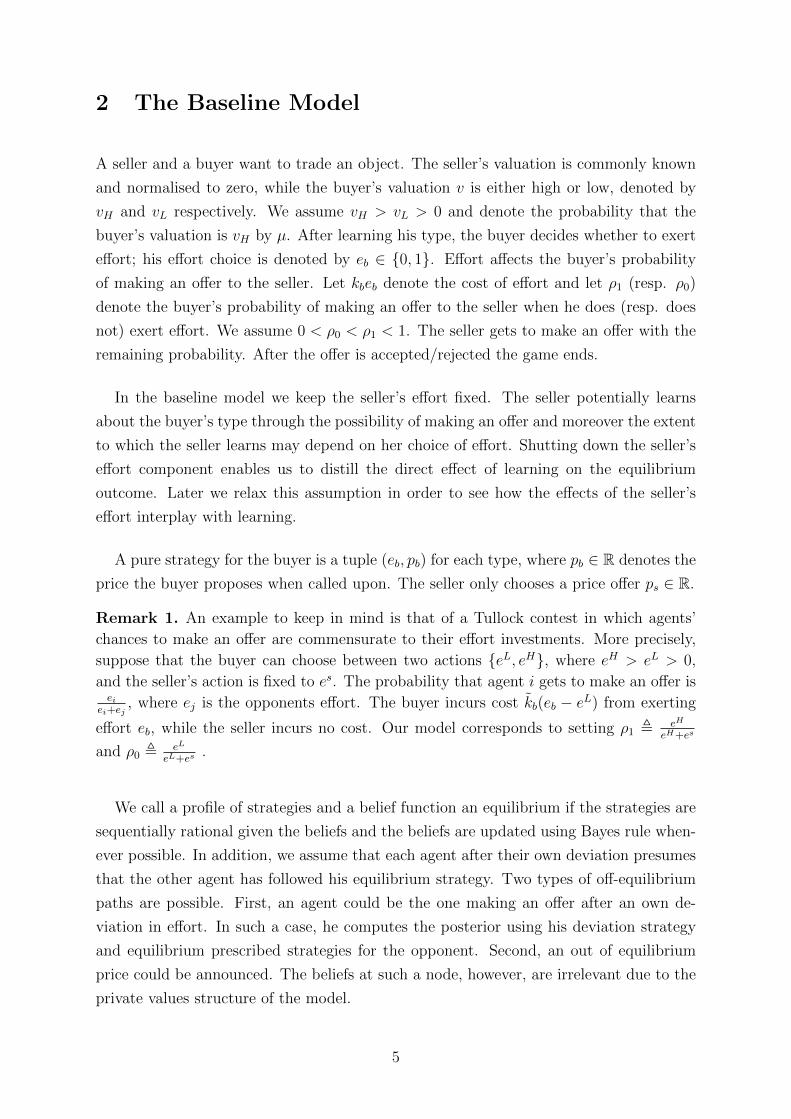
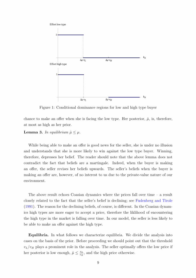
on the seller’s expected price; see Figure 1. The above analysis can be synthesized as
follows.
Lemma 2. Exerting effort is conditionally dominant for both types of buyer if kb < ∆ρ vL,
while not exerting effort is conditionally dominant for the low type buyer if kb > ∆ρ vLand for the high type buyer if kb > ∆ρ vH .
To sum up, when effort costs are sufficiently high or low, both types of buyer take the
same effort decision, regardless of the seller’s behavior. On the other hand, when the cost
of effort is in the intermediate region,
∆ρ vL ≤ kb ≤ ∆ρ vH ,
the low type buyer optimally refrains from exerting effort, whereas the high type’s optimal
effort decision depends on the expected price the seller charges when making the offer.
The fact that the low type never exerts effort with a higher probability than the high
type has consequences for the seller’s behavior. If the seller believes that type vi exerts
effort with probability βi (i = L,H) and the seller gets to make the offer herself, her
posterior belief that the buyer is of high type is
µ ,µ [βH(1− ρ1) + (1− βH)(1− ρ0)]
µ [βH(1− ρ1) + (1− βH)(1− ρ0)] + (1− µ) [βL(1− ρ1) + (1− βL)(1− ρ0)],
where βH(1 − ρ1) + (1 − βH)(1 − ρ0) is the probability that the seller wins against the
high type, and βL(1 − ρ1) + (1 − βL)(1 − ρ0) the probability that she wins against the
low type. Since the high type buyer is more likely to exert effort, that is βH ≥ βL, he is
also the one who is more likely to make an offer. In other words, the seller has a higher
8
DΡ vHDΡ vL
kb
1
Effort low type
DΡ vHDΡ vL
kb
1
Effort high type
Figure 1: Conditional dominance regions for low and high type buyer
chance to make an offer when she is facing the low type. Her posterior, µ, is, therefore,
at most as high as her prior.
Lemma 3. In equilibrium µ ≤ µ.
While being able to make an offer is good news for the seller, she is under no illusion
and understands that she is more likely to win against the low type buyer. Winning,
therefore, depresses her belief. The reader should note that the above lemma does not
contradict the fact that beliefs are a martingale. Indeed, when the buyer is making
an offer, the seller revises her beliefs upwards. The seller’s beliefs when the buyer is
making an offer are, however, of no interest to us due to the private-value nature of our
environment.
The above result echoes Coasian dynamics where the prices fall over time – a result
closely related to the fact that the seller’s belief is declining; see Fudenberg and Tirole
(1991). The reason for the declining beliefs, of course, is different. In the Coasian dynam-
ics high types are more eager to accept a price, therefore the liklihood of encountering
the high type in the market is falling over time. In our model, the seller is less likely to
be able to make an offer against the high type.
Equilibria. In what follows we characterize equilibria. We divide the analysis into
cases on the basis of the prior. Before proceeding we should point out that the threshold
vL/vH plays a prominent role in the analysis. The seller optimally offers the low price if
her posterior is low enough, µ ≤ vLvH
, and the high price otherwise.
9
We start with the case where the seller’s prior is low: µ ≤ vL/vH .
Proposition 1. If µ ≤ vLvH
, there is a generically unique equilibrium with the property
that both types of buyer undertake the same effort choice and the seller offers price vL.
The seller’s decision to offer price vL is a consequence of Lemma 3: if her prior is
below the threshold vL/vH , her posterior will be below the threshold too. Moreover, once
the seller is charging the low price, Lemma 1 implies that both types of buyer have the
same incentive to exert effort and, therefore, make the same effort choice. The seller, in
turn, learns nothing from gaining the opportunity to make an offer. Her posterior thus
coincides with her prior.6
Next, we turn attention to high seller’s priors: µ > vL/vH . Lemma 2 established that
both types of buyer make the same effort choice when the cost of effort is extreme—either
very high or very low. In those cases, the two types have the same dominant strategy
and the seller cannot infer anything from the bargaining process. She, therefore, offers
the high price.
Proposition 2. Let kb ≤ ∆ρ vL or kb ≥ ∆ρ vH and µ > vL/vH . In the (generically)
unique equilibrium both types of the buyer make the same effort choice and the seller
offers price vH .
The seller learns. Hereafter we focus on the environment in which the high type
buyer’s optimal effort choice depends on the seller’s behavior, that is, when the buyer’s
cost is intermediate:
∆ρ vL < kb < ∆ρ vH .
As a reminder, in this region the low type buyer prefers to exert low effort, while the
high type buyer’s optimal effort decision depends on the price he expects the seller to
charge. The potential difference in the strategies of the two types of buyer gives rise to
a possibility for the seller to learn about her competitor. To this end, we will maintain
the assumption µ > vLvH
, so that if the seller were to learn nothing, she would optimally
propose the separating price vH .
Before stating the result, it is useful to define additional notation. Let
m ,(1− ρ0) vL
vH
(1− ρ0) vLvH
+ (1− ρ1)(1− vLvH
), (4)
6 Genericity in the above proposition refers to the case where both types of buyer are indifferentbetween exerting effort and not exerting effort when the seller is expected to offer the low price.
10
be the prior belief such that if the high type buyer exerts effort and the low type does
not, the seller’s posterior is precisely vL/vH . As a consequence, for all priors above m, the
seller’s posterior will be above the threshold vL/vH , regardless of the buyer’s behavior,
and the seller optimally offers price vH .
Proposition 3. Let kb ∈ (∆ρ vL,∆ρ vH) and µ > vLvH
. There is a unique equilibrium:
• when µ < m, the high type buyer exerts effort with probability βH = (1−ρ0)(µvH−vL)∆ρµ(vH−vL)
and the low type exerts no effort; the seller offers price vH with probability σ =kb−∆ρ vL
∆ρ(vH−vL);
• when µ ≥ m, the high type buyer exerts effort and the low type does not; the seller
offers price vH .
The equilibrium exhibits the most interesting behavior when the prior is only slightly
above the threshold vLvH
; more precisely, when the prior is between vLvH
and m. If the seller
was to learn nothing during bargaining, she would offer the high price vH . In anticipation
of the seller’s behavior, the high type buyer would find it optimal to exert effort, while
the low type buyer would not. The seller should then revise her beliefs downward and
optimally offer the low price vL. Foreseeing the seller’s intention to offer the low price
neither type of the buyer would have an incentive to exert effort. But then the seller
would not learn, and, completing the circle, would want to offer the high price.
To prevent such cycling of beliefs, the high type buyer randomizes between exerting
and not exerting effort in such a way that the seller is indifferent between the two prices,
that is, in such a way that the seller’s posterior is precisely vL/vH ; this pins down βH . The
probability of the high type exerting effort is strictly increasing in the prior in the relevant
region. Namely, the higher the prior, the larger must be the difference in expectation
between the low and the high type’s effort to bring the seller’s posterior down to vL/vH .
The seller, on the other hand, offers the high price with the probability that makes the
high type buyer indifferent between the two efforts. The high type’s indifference delivers
the seller’s probability of charging the high price, σ. Notice that the latter is independent
of the prior; after all, it is determined by the high type’s indifference.
As stated above, for the priors above m the seller’s posterior will be above the threshold
vL/vH . The seller, therefore, offers the high price, which sets a strong incentive for the
high type buyer to make the offer himself. Consequently, he exerts effort with certainty.
This covers the second bullet point in the above result.
11
2.2 Comparative Statics
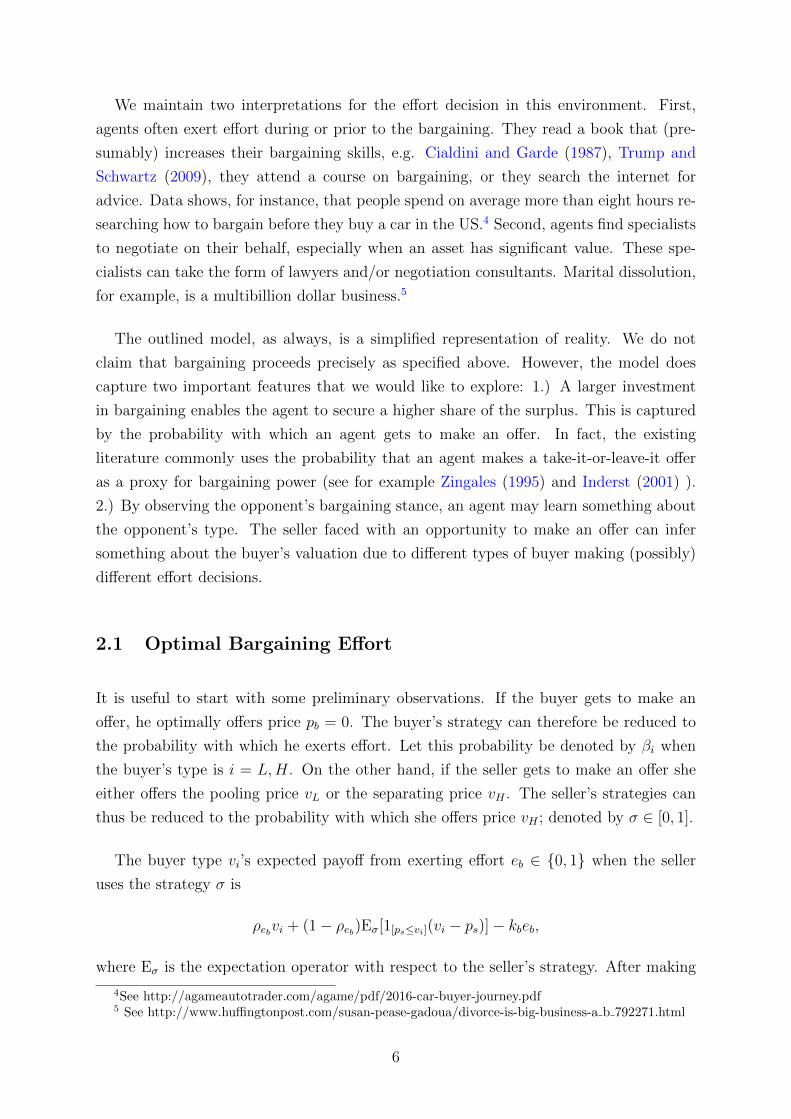
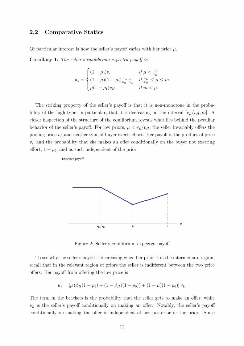
Of particular interest is how the seller’s payoff varies with her prior µ.
Corollary 1. The seller’s equilibrium expected payoff is
us =
(1− ρ0)vL if µ < vL
vH
(1− µ)(1− ρ0) vLvHvH−vL
if vLvH≤ µ ≤ m
µ(1− ρ1)vH if m < µ.
The striking property of the seller’s payoff is that it is non-monotone in the proba-
bility of the high type, in particular, that it is decreasing on the interval [vL/vH ,m]. A
closer inspection of the structure of the equilibrium reveals what lies behind the peculiar
behavior of the seller’s payoff. For low priors, µ < vL/vH , the seller invariably offers the
pooling price vL and neither type of buyer exerts effort. Her payoff is the product of price
vL and the probability that she makes an offer conditionally on the buyer not exerting
effort, 1− ρ0, and as such independent of the prior.
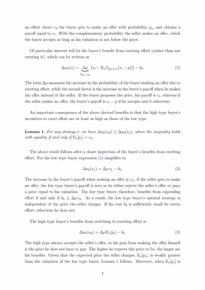
vL �vH m 1Μ
Expected payoff
Figure 2: Seller’s equilibrium expected payoff
To see why the seller’s payoff is decreasing when her prior is in the intermediate region,
recall that in the relevant region of priors the seller is indifferent between the two price
offers. Her payoff from offering the low price is
us = [µ (βH(1− ρ1) + (1− βH)(1− ρ0)) + (1− µ)(1− ρ0)] vL.
The term in the brackets is the probability that the seller gets to make an offer, while
vL is the seller’s payoff conditionally on making an offer. Notably, the seller’s payoff
conditionally on making the offer is independent of her posterior or the prior. Since
12
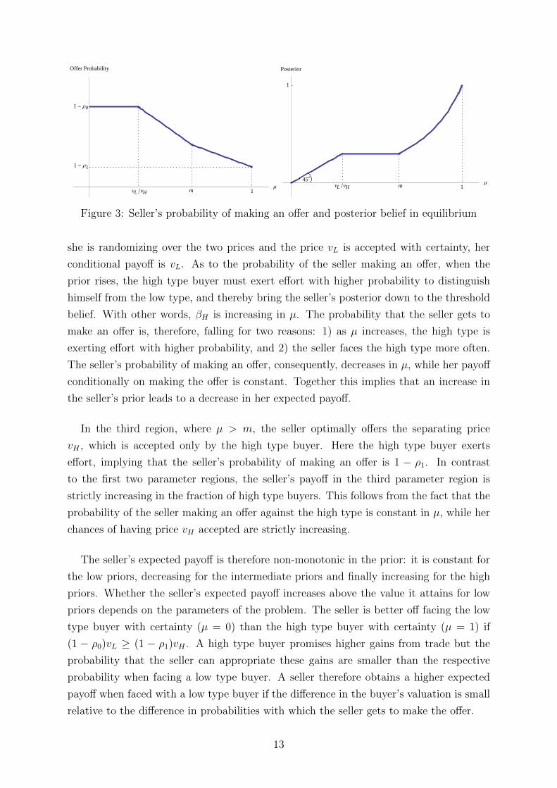
vL �vH m
1 - Ρ0
1 - Ρ1
1Μ
Offer Probability
vL �vH m45ë
1Μ
1
Posterior
Figure 3: Seller’s probability of making an offer and posterior belief in equilibrium
she is randomizing over the two prices and the price vL is accepted with certainty, her
conditional payoff is vL. As to the probability of the seller making an offer, when the
prior rises, the high type buyer must exert effort with higher probability to distinguish
himself from the low type, and thereby bring the seller’s posterior down to the threshold
belief. With other words, βH is increasing in µ. The probability that the seller gets to
make an offer is, therefore, falling for two reasons: 1) as µ increases, the high type is
exerting effort with higher probability, and 2) the seller faces the high type more often.
The seller’s probability of making an offer, consequently, decreases in µ, while her payoff
conditionally on making the offer is constant. Together this implies that an increase in
the seller’s prior leads to a decrease in her expected payoff.
In the third region, where µ > m, the seller optimally offers the separating price
vH , which is accepted only by the high type buyer. Here the high type buyer exerts
effort, implying that the seller’s probability of making an offer is 1 − ρ1. In contrast
to the first two parameter regions, the seller’s payoff in the third parameter region is
strictly increasing in the fraction of high type buyers. This follows from the fact that the
probability of the seller making an offer against the high type is constant in µ, while her
chances of having price vH accepted are strictly increasing.
The seller’s expected payoff is therefore non-monotonic in the prior: it is constant for
the low priors, decreasing for the intermediate priors and finally increasing for the high
priors. Whether the seller’s expected payoff increases above the value it attains for low
priors depends on the parameters of the problem. The seller is better off facing the low
type buyer with certainty (µ = 0) than the high type buyer with certainty (µ = 1) if
(1 − ρ0)vL ≥ (1 − ρ1)vH . A high type buyer promises higher gains from trade but the
probability that the seller can appropriate these gains are smaller than the respective
probability when facing a low type buyer. A seller therefore obtains a higher expected
payoff when faced with a low type buyer if the difference in the buyer’s valuation is small
relative to the difference in probabilities with which the seller gets to make the offer.
13
Finally, notice that the case for the seller’s payoff being decreasing could have been
made even in the environment with perfect information. This is the case when the seller’s
payoff at µ = 1 is smaller than at µ = 0. However, our result is stronger than that: even
when the seller’s payoff at µ = 1 is larger than at µ = 0, there is always an intermediate
region of priors under which the seller is strictly worse off than when she faces the low
value buyer with certainty.
The non-monotonicity of the seller’s expected payoff stands in stark contrast to models
where the probability of each agent making an offer is exogenously determined and fixed
over types; more about this in Section 4.2. The fact that the seller’s payoff can be
decreasing in the probability of the high type has potentially interesting implications for
applied work. Suppose that the seller has to decide on entering one of two markets:
the first populated almost exclusively by low value buyers, the second consisting of a
fair share of high value customers. The above non-monotonicity result shows that the
seller might indeed prefer to enter the market with low value customers and go for the
proverbial low hanging fruit. The higher proportion of the high value buyers offers higher
surplus to be split between the two parties. However, the high value buyers fight harder
for the said surplus, which can result in a worse outcome for the seller.
3 Two-Sided Effort
We now augment the analysis with the possibility of the seller exerting effort es ∈ {0, 1}at a cost kses. The seller’s effort, in addition to affecting the probability with which
the seller gets to make an offer, plays a prominent role in the seller’s learning about
the buyer’s valuation. We show that this interaction gives rise to novel and interesting
equilibrium behavior.
We assume that the probability of making an offer as a function of the buyer’s and
seller’s effort choice takes the following simple form:ρ if ei > e−i,12
if ei = e−i,
1− ρ if ei < e−i,
where ρ ∈ (12, 1). The effect of effort on the probability of making an offer is symmetric
for the buyer and the seller, while differences in bargaining skills are captured by the
relative costs of effort. Similarly as in the previous section, a canonical example of our
environment is a Tullock contest, though here both agents face effort choices.
14
3.1 Equilibrium Analysis
The seller optimally chooses a price ps from the set {vL, vH}. Her strategy can, therefore,
be described by a probability distribution σ over pairs (es, ps) with es ∈ {0, 1} and
ps ∈ {vL, vH}. The buyer optimally offers a price equal to zero, thus his decision problem
boils down to the choice of effort.
We start again by considering the buyer’s benefit from exerting effort. Notice that the
increase in the probability with which the buyer gets to make an offer when switching
to exerting effort does not depend on whether or not the seller exerts effort: ∆ρ =12− (1− ρ) = ρ− 1
2. The high type buyer’s benefit from exerting effort can therefore be
written as
∆ub(vH) , Prσ[es = 1]Eσ [∆ρ ps − kb|es = 1] + Prσ[es = 0]Eσ [∆ρ ps − kb | es = 0]
= ∆ρEσ[ps]− kb,
exactly as in Section 2. Similarly, for the low type buyer:
∆ub(vL) , ∆ρ vL − kb.
Due to the fact that the buyer’s benefit of exerting effort does not depend on the seller’s
effort choice, some of the lemmata that we developed in Section 2 carry over to this
environment. In particular, the high type buyer has at least as high an incentive to exert
effort as the low type. This implies that (generically) the high type buyer exerts effort
with at least as high probability as the low type. Another implication, corresponding to
Lemma 3, is that the seller’s posterior is never above her prior.
The seller’s benefit of exerting effort when planning to offer a price ps is:
∆us(ps) = ∆ρ [µps + (1− µ)1[p=vL]ps]− ks. (5)
As before, the term ∆ρ captures the increase in probability that the seller gets to make
the offer when she switches to exerting effort. This increase does not depend on whether
the buyer exerts effort or not. The seller’s optimal effort choice is, therefore, determined
by the price she intends to propose. At the same time, it does not directly depend on
the buyer’s behavior. The seller’s optimal pricing strategy, and through that her effort,
however, will depend on the buyer’s conduct. Vice versa, the seller’s choice of effort affects
how much she learns about the buyer and, as a result, her optimal pricing strategy.
Lemma 4. When the high type buyer exerts effort with a higher probability than the low
type, the seller’s posterior µ is smaller when es = 0 than when es = 1.
15

Exerting effort diminishes the extent to which the seller updates her belief, i.e., learns.
All else equal exerting effort favors the separating price vH . More precisely, if after not
exerting effort the seller optimally offers vH , she prefers price vH also after exerting effort.
This has important implications for the equilibrium characterization that follows next.
When the seller’s cost of effort is sufficiently extreme, she has a dominant effort choice.
In particular, if ks > ∆ρ vH , the benefit from exerting effort is negative regardless of the
seller’s prior and her choice of prices. The equilibrium analysis of Section 2, where the
seller’s effort choice was absent, applies after setting ρ1 = ρ and ρ0 = 12. Similarly, if
ks < ∆ρ vL, the seller optimally exerts effort for all µ. The equilibrium analysis of Section
2 can be applied with the parameters ρ1 = 12
and ρ0 = 1−ρ. These cases are summarised
in the following proposition.
Proposition 4. The equilibrium is generically unique and satisfies the following proper-
ties:
• If ks ≤ ∆ρ vL, the seller exerts effort and the seller’s pricing strategy as well as
the buyer’s effort strategy are described by Propositions 1-3 with ρ1 = 1/2 and
ρ0 = 1− ρ.
• If ks ≥ ∆ρ vH , the seller exerts no effort and the seller’s pricing strategy as well
as the buyer’s effort strategy are described by Propositions 1-3 with ρ1 = ρ and
ρ0 = 1/2.
More elaborate, and interesting, is the analysis of the case where the seller does have
an incentive to change her effort choice with the prior. In addition, we restrict attention
to the case where the two types of buyer do not have the a dominant effort choice, so
that learning is indeed possible. All together, kb, ks ∈ (∆ρ vL,∆ρ vH).
We can show that there is a threshold prior such that below this threshold the seller
refrains from effort regardless of the buyer’s behavior, then we determine the behav-
ior above this threshold. The relevant threshold, mH(ks), is the prior at which the
seller is indifferent between exerting effort and not when she charges the high price:
∆ρmH(ks)vH − ks = 0,7 or differently
mH(ks) =ks
∆ρ vH. (6)
For µ ≤ mH(ks) the analysis from Section 2 then carries over with the seller exerting no
effort; that is, ρ1 = ρ and ρ0 = 12.
7For µ ≥ vL/vH , the seller is more likely to exert effort when planing to charge the high price andunder higher priors.
16
Recall that, in the environment without the seller’s effort choice, the seller’s pricing
decision was to offer the low price for low priors, randomize over the two prices at inter-
mediate priors and offer the high price for high priors. Given ρ1 = ρ and ρ0 = 12, the
threshold between the last two regions, as determined in (4), is given by
m0 =12vLvH
12vLvH
+ (1− ρ)(1− vLvH
).
Given that mH(ks) is the threshold where the seller wants to switch to exerting effort
when planning to offer the high price, we break the analysis into the cases when it falls
in the region below m0, where the seller randomizes over prices, or above m0, where the
seller offers the high price (when not exerting effort).8
We start with the latter case, mH(ks) > m0. Here just below mH(ks) the high type
buyer exerts effort and the seller offers the high price after not exerting effort. At the prior
mH(ks) the seller switches to expending effort. Her posterior jumps upwards (see Lemma
3), implying that the seller indeed prefers to offer the high price. Since the buyer’s effort
choice does not depend on the seller’s, the buyer’s behavior remains optimal. To sum up,
for µ ≥ mH(ks) the seller exerts effort and offers price vH , while for the remaining values
of µ the equilibrium is as characterized in Proposition 3 when the seller does not exert
effort. The following proposition summarizes this analysis.
Proposition 5. Let kb, ks ∈ (∆ρ vL,∆ρ vH) and mH(ks) > m0. There is a generically
unique equilibrium with the following properties:
• if µ ≤ vLvH
, nobody exerts effort and the seller offers the low price;
• if vLvH
< µ ≤ m0, the high type buyer randomizes over the two effort choices, the
seller does not exert effort and randomizes over the two prices;
• if m0 < µ < mH(ks), the high type buyer exerts effort, while the seller does not; the
seller offers price vH ;
• it mH(ks) ≤ µ, the seller and the high type exert effort, and moreover, the seller
offers price vH .
The low type buyer never exerts effort.
It remains to investigate the case where mH(ks) falls into region where the seller would
randomize over prices after not exerting effort, mH(ks) ∈ (vL/vH ,m0). For priors just
8Given the assumptions on ks and kb, mH(ks) > vL/vH .
17
below mH(ks) the seller not exerting effort and randomizing over prices remains the only
equilibrium. At the threshold mH(ks) the seller would, however, prefer to exert effort if
she intended to offer the high price but not if she wanted to offer the low price. Moreover,
since just below mH(ks) the seller is randomizing over the prices, she must be indifferent
between the tuples (0, vL) and (0, vH). By definition of mH(ks), at the threshold the
tuple (1, vH) becomes preferable to (0, vH), presenting a profitable deviation from the
equilibrium with randomization over prices. Thus, the strategy profile where the seller
exerts effort and charges the high price becomes the natural candidate for equilibrium
above mH(ks). In that case, the high type buyer would optimally exert effort as well.
This is an equilibrium only if the seller has no incentives to deviate to not exerting effort
and offering the low price. That is, if
µ1
2vH − ks ≥
(µ(1− ρ) + (1− µ)
1
2
)vL.
Letting m(ks) denote the prior at which the above condition is satisfied with equality, the
described equilibrium exists for all µ ≥ m(ks). Under the assumed parameter conditions,
the threshold m(ks) is strictly larger than mH(ks). This implies that there is an additional
parameter region, between mH(ks) and m(ks), where there is no equilibrium in which the
seller has a fixed effort. This brings about a rather interesting new type of behavior.
Proposition 6. Assume kb, ks ∈ (∆ρ vL,∆ρ vH) as well as mH(ks) < m0. There is a
generically unique equilibrium with the following properties:
• if µ ≤ vLvH
, nobody exerts effort and the seller offers the low price;
• if vLvH
< µ ≤ mH(ks), the high type buyer randomizes over the two effort choices,
the seller does not exert effort and randomizes over the two prices;
• if mH(ks) < µ < m(ks), the high type buyer randomizes over the two effort choices,
while the seller randomizes over the two pairs (0, vL) and (1, vH);
• for m(ks) ≤ µ, the high type buyer and the seller exert effort and the seller offers
the high price;
where m(ks) =ks+ 1
2vL
12vH+∆ρ vL
. In all cases the low type buyer does not exert effort.
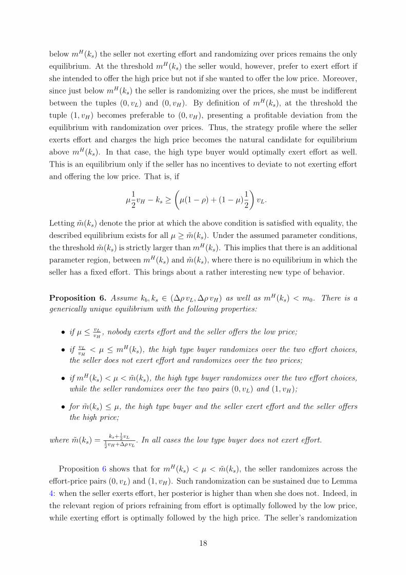
Proposition 6 shows that for mH(ks) < µ < m(ks), the seller randomizes across the
effort-price pairs (0, vL) and (1, vH). Such randomization can be sustained due to Lemma
4: when the seller exerts effort, her posterior is higher than when she does not. Indeed, in
the relevant region of priors refraining from effort is optimally followed by the low price,
while exerting effort is optimally followed by the high price. The seller’s randomization
18
preserves the expected price, leaving the high type buyer indifferent between the two
effort choices. The high type buyer, in response, adjusts his randomization to make the
seller indifferent. In contrast to the case when µ is just below mH(ks), the probability
with which the buyer exerts effort does not make the seller indifferent between prices for
a given effort but instead between the two strategies (0, vL) and (1, vH). The threshold
m(ks) is the highest prior at which the seller can indeed be made indifferent between the
two effort-price pairs.
3.2 Comparative Statics
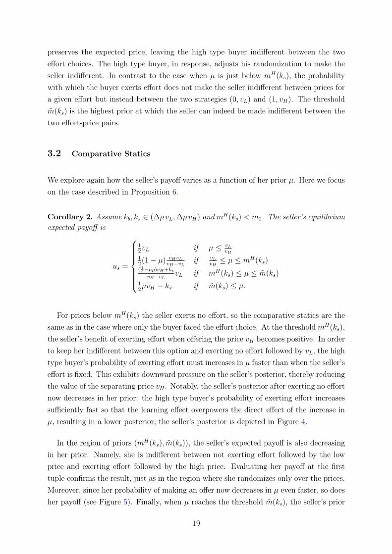
We explore again how the seller’s payoff varies as a function of her prior µ. Here we focus
on the case described in Proposition 6.
Corollary 2. Assume kb, ks ∈ (∆ρ vL,∆ρ vH) and mH(ks) < m0. The seller’s equilibrium
expected payoff is
us =
12vL if µ ≤ vL
vH12(1− µ) vHvL
vH−vLif vL
vH≤ µ ≤ mH(ks)
( 12−µρ)vH+ksvH−vL
vL if mH(ks) ≤ µ ≤ m(ks)12µvH − ks if m(ks) ≤ µ.
For priors below mH(ks) the seller exerts no effort, so the comparative statics are the
same as in the case where only the buyer faced the effort choice. At the threshold mH(ks),
the seller’s benefit of exerting effort when offering the price vH becomes positive. In order
to keep her indifferent between this option and exerting no effort followed by vL, the high
type buyer’s probability of exerting effort must increases in µ faster than when the seller’s
effort is fixed. This exhibits downward pressure on the seller’s posterior, thereby reducing
the value of the separating price vH . Notably, the seller’s posterior after exerting no effort
now decreases in her prior: the high type buyer’s probability of exerting effort increases
sufficiently fast so that the learning effect overpowers the direct effect of the increase in
µ, resulting in a lower posterior; the seller’s posterior is depicted in Figure 4.
In the region of priors (mH(ks), m(ks)), the seller’s expected payoff is also decreasing
in her prior. Namely, she is indifferent between not exerting effort followed by the low
price and exerting effort followed by the high price. Evaluating her payoff at the first
tuple confirms the result, just as in the region where she randomizes only over the prices.
Moreover, since her probability of making an offer now decreases in µ even faster, so does
her payoff (see Figure 5). Finally, when µ reaches the threshold m(ks), the seller’s prior
19
vL �vH 1
Posterior : es = 1
Posterior : es = 0
m� Hks LmH Hks L
Μ
Posterior
Figure 4: Seller’s equilibrium posterior after exerting and not exerting effort
mH Hks L m� Hks LvL �vH 1
Μ
1
Effort high type
vL �vH 1m� Hks LmH Hks L
Μ
Expected payoff
Figure 5: High type buyer’s effort and seller’s expected payoff in equilibrium
is sufficiently high so that she and the high type buyer exert effort with probability one.
From here on the seller’s payoff is again increasing.
4 Discussion
4.1 Effort Costs and Welfare
In what follows we will discuss how total surplus depends on the effort cost parameters
kb and ks. The two parameters affect the probability with which either party exerts effort
in equilibrium and through that welfare. As can be verified from Propositions 4-6, the
seller’s and buyer’s equilibrium efforts are non-increasing in their own costs, ks and kb.
However, since the probability with which agents exert effort in equilibrium varies with
the cost parameters in a non-continuous way, effects on welfare are rather erratic. Instead
20
of giving a full account, we focus on three important channels through which effort costs
influence welfare.
The first channel is the direct effect of an increase in ks or kb on the total cost of effort
that is incurred in equilibrium. As long as an increase in the cost of effort does not lead
to a change of the equilibrium effort choice of the respective agent, such increase clearly
lowers total surplus. A higher effort cost might, however, deter an agent from exerting
effort, thus lowering the incurred cost of effort and potentially increasing welfare. The
realized equilibrium effort costs for agent i = b, s are therefore lowest either when ki
vanishes or when ki is sufficiently large.
The second channel comes from the one-sidedness of the private information in our
model. If the buyer was always the one to make an offer, trade would take place with
probability one and the gains from trade would be maximized. In contrast, when the
seller makes an offer, she sometimes finds it optimal to offer the separating price vH ,
thereby forgoing the possibility of trade with the low type buyer. By implication, the
realized gains from trade cannot decrease when the probability that the buyer makes an
offer increases; all else equal. This channel therefore suggests that the realized gains from
trade are greater when the buyer’s cost of effort is small relative to the seller’s.
Lastly, effort costs have an indirect effect on how much the seller learns in equilibrium.
Lemma 4 shows that the seller’s posterior is lower when she exerts no effort. This makes
her more likely to charge the pooling price vL, which, holding the buyer’s effort fixed,
increases trading surplus. Given that the seller’s equilibrium effort decreases in her cost,
this implies that a higher value of ks not only makes it more likely for the buyer to make
an offer but also less likely that trade is forgone in case the seller makes an offer. The
three channels imply that surplus is maximal when kb is small and ks is large.
Finally, we want to point out that an increase in ks can lead to an increase in total
surplus also when the seller’s equilibrium effort choice does not change. Even more
perplexing, not only surplus but also the seller’s payoff can increase with ks. This effect
arises in the parameter region where the seller randomizes across the pairs of strategies
(0, vL) and (1, vH); see Proposition 6. In this region the buyer’s payoff does not depend
on the seller’s cost parameter since the seller’s randomization between (0, vL) and (1, vH)
is independent of ks.9 On the other hand, the seller’s expected payoff, given by
us =(1
2− µρ)vH + ks
vH − vLvL,
is increasing in ks; see Corollary 2. To gain some intuition for why this is the case, notice
9The seller randomizes to keep the buyer indifferent, who clearly does not care about ks.
21
that, as ks increases, exerting effort and offering the high price becomes less attractive
for the seller. As a consequence, the high type buyer can exert effort with a smaller
probability, without violating the seller’s indifference condition. This implies that the
payoff associated to exerting no effort and offering the low price must increase: the seller
incurs no cost but gets to make an offer with a strictly higher probability. In equilibrium
the payoff from choosing (0, vL) is equal to the one from choosing (1, vH), which means
that also the latter increases. The positive effect on the probability of making an offer
therefore outweighs the higher effort cost the seller incurs. It follows that the seller’s
expected payoff (and in consequence total surplus) strictly increases in ks.
4.2 Probabilistic Bargaining Model
The probabilistic bargaining model is a model in which the buyer and the seller get to
make an offer with a fixed probability. Unlike in the above proposed model, the proba-
bility of making an offer is exogenously given and independent of the agents’ valuations.
Such models are commonly used in economics and finance; for examples see Inderst
(2001) and Zingales (1995), though probabilistic bargaining goes back at least to Rubin-
stein and Wolinsky (1985). Since these models are much simpler than our model with
endogenous probabilities of making an offer, one might wonder whether a generalization
of the probabilistic bargaining model could capture some of the interesting feature of our
model.
More formally, suppose that in a probabilistic model of bargaining the buyer’s and the
seller’s valuations are as above. When they meet, the buyer gets to make an offer with
probability ρ and the seller with the remaining probability; the probability reflects the
buyer’s bargaining power. If the offer is rejected the game ends. Securing the right to
make an offer conveys no information to the seller. She, therefore, makes the offer on the
basis of her prior distribution, she offers the high price if her prior is above vL/vH and the
low price otherwise. This model corresponds to the model presented in previous sections
only in the case where not exerting effort is the dominant strategy for both players. The
cases where both players have dominant strategies, but one or both players exert effort,
are quite similar too with the difference that in our model some surplus is burnt due to
the cost of effort. The interesting properties, like learning and non-monotonicity of the
seller’s payoff, however, cannot be replicated with the simple probabilistic model.
Our model with efforts showed that high value buyers have a higher propensity to exert
effort and through that higher bargaining power. To capture this feature we propose a
richer version of the probabilistic bargaining model in which the high type buyer gets to
22
make an offer with probability ρH and the low type with probability ρL, where ρH > ρL.
The following proposition characterizes the equilibrium.
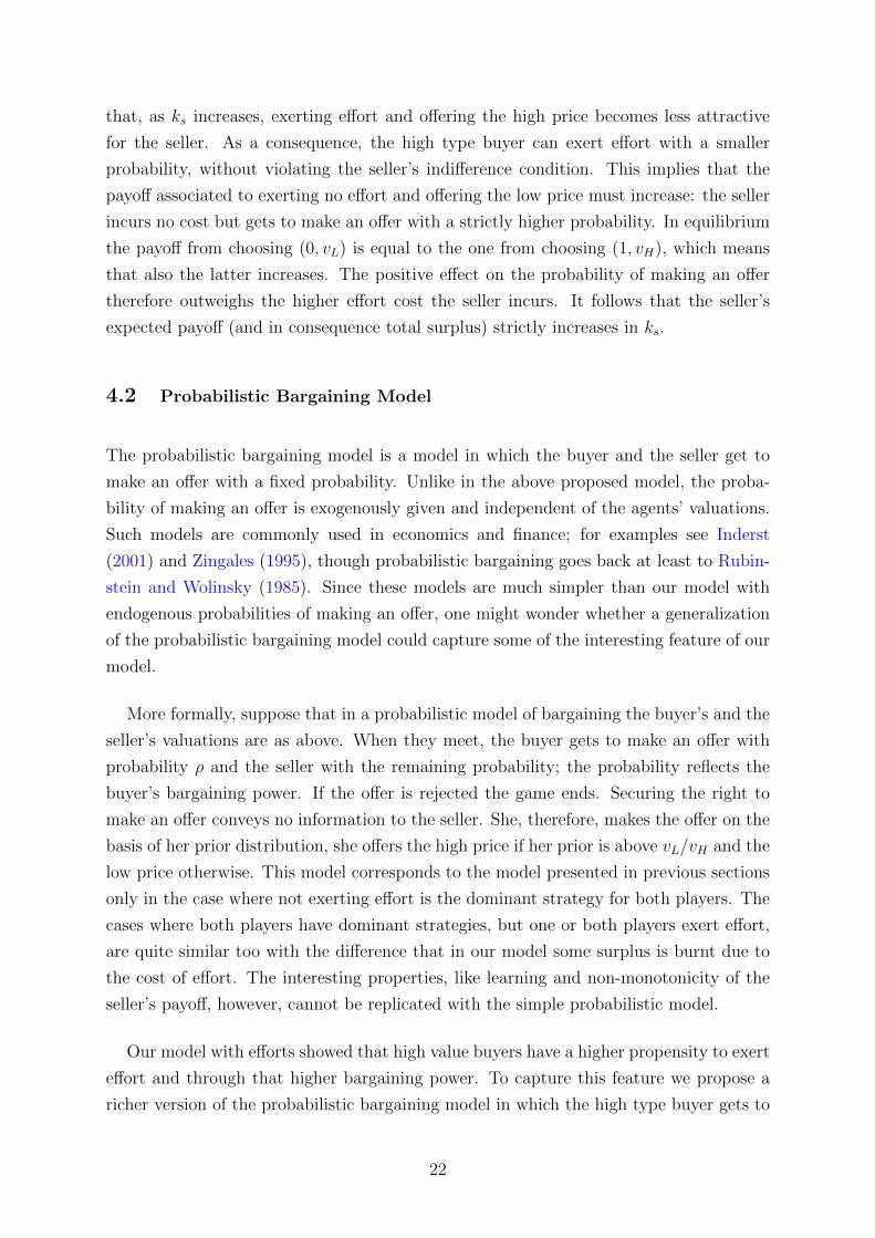
Proposition 7. The seller optimally offers the high price if
µ ≥(1− ρL) vL
vH
(1− ρH)(1− vLvH
) + (1− ρL) vLvH︸ ︷︷ ︸
,µ∗
(7)
and the low price otherwise.
It is easy to see that the seller’s threshold µ∗ (the right hand side of the above inequal-
ity) is larger than vL/vH . Being given the opportunity to make an offer is a negative
signal for the seller; she has an easier time making an offer against the low type. Win-
ning the chance to make an offer, therefore, lowers her belief. Consequently, she is willing
to offer the high price only when her prior sufficiently favors the high type.
To highlight the comparison between the probabilistic bargaining model with varying
bargaining power and our model with efforts, we examine how the seller’s payoff changes
with the prior.
Corollary 3. The seller’s equilibrium expected payoff is
us =
{[µ(1− ρH) + (1− µ)(1− ρL)]vL if µ ≤ µ∗
µ(1− ρH)vH if µ > µ∗.
H1 - ΡH L vHH1 - ΡL L vL
Μ* 1Μ
Expected payoff
Figure 6: Seller’s equilibrium payoff: random proposal model
23
The assumption ρH > ρL implies that the seller’s payoff is decreasing as long as
µ ≤ µ∗ and increasing for µ > µ∗. In the region of low priors the seller offers price vL
and both types accept it. The seller, however, suffers from the incidence of high types,
as this decreases her probability of making an offer. This property is different from our
model where the probability of making an offer is endogenously determined. In the latter
model, when expecting the low price, both types of buyer make the same effort choice,
and therefore, win with the same probability against the seller. In the region of high
priors where the seller charges the high price, the occurrence of high types also decreases
her chances of making an offer. The effect is, however, overpowered by the fact that the
seller’s price offer is accepted more often. The sum of the two effects is an unequivocal
benefit of facing more high types for the seller.
The version of the probabilistic bargaining model with different probabilities for dis-
tinct types approximates the model with efforts relatively well. In particular, it captures
the non-monotonicity of the seller’s payoff. It does not match it exactly, though, the main
distinction being that in the model with effort the difference between the probabilities of
the high and the low type making an offer endogenously increases in the prior. Among
other things, this accounts for the difference between the two models in the seller’s payoff
below the threshold vL/vH . Despite the differences between the two models, we find that
a researcher who wishes to use a more manageable format will be well suited with the
probabilistic model proposed here.
5 Concluding Remarks
We propose a model that endogenizes bargaining power in a bilateral trade environment
through costly effort. We show that higher types endogenously acquire higher bargaining
power. Interestingly, this can lead to the seller’s payoff being non-monotonic in the
proportion of high value buyers. Therefore, if the seller were to choose between the entry
into two markets, one with a low proportion of high value customers, the other with a
higher, she might choose the one with the lower incidence of high value customers. While
the high value buyers offer a higher potential surplus, they also more actively negotiate
the terms of trade. The two countervailing incentives can drive the seller to pick the
market that is predominantly populated by low value customers—the seller focuses on
the low hanging fruit.
Flexibility of our model offers several avenues for future research. Worthy of scrutiny
might be the environment where efforts are observable, and thus serve as a signalling
24
device. One might also wonder how the seller’s private information would influence
bargaining. We plan to explore these models in future work.
6 Appendix
Proof of Lemma 1. The result follows from the comparison of (3) and (2), and the fact
that Eσ[p] ≥ vL, that is, the seller never offers a price below vL.
Proof of Lemma 2. The result is argued in the text preceding the statement of the
lemma.
Proof of Lemma 3. The seller’s posterior can be written as
µ =µ [βH(1− ρ1) + (1− βH)(1− ρ0)]
µ [βH(1− ρ1) + (1− βH)(1− ρ0)] + (1− µ) [βL(1− ρ1) + (1− βL)(1− ρ0)]
≤ µ [βH(1− ρ1) + (1− βH)(1− ρ0)]
µ [βH(1− ρ1) + (1− βH)(1− ρ0)] + (1− µ) [βH(1− ρ1) + (1− βH)(1− ρ0)]
= µ,
where the inequality follows from βH ≥ βL and ρ1 > ρ0.
Proof of Proposition 1. Due to Lemma 3, we know that µ < vL/vH implies µ <
vL/vH . Conditional on making an offer, the seller thus strictly prefers the pooling price
vL. Given this, we have ∆ub(vL) = ∆ub(vH), so that the low type buyer optimally exerts
effort if and only if the high type optimally exerts effort.
Proof of Proposition 2. Under the stated conditions, both types of buyer undertake
the same effort choice. This implies that when the seller gets to make the offer her
posterior is equal to her prior µ. If µ is smaller (greater) than vL/vH , the payoff associated
to the pooling price, vL, is greater (smaller) than the payoff associated to the separating
price, µvH .
25
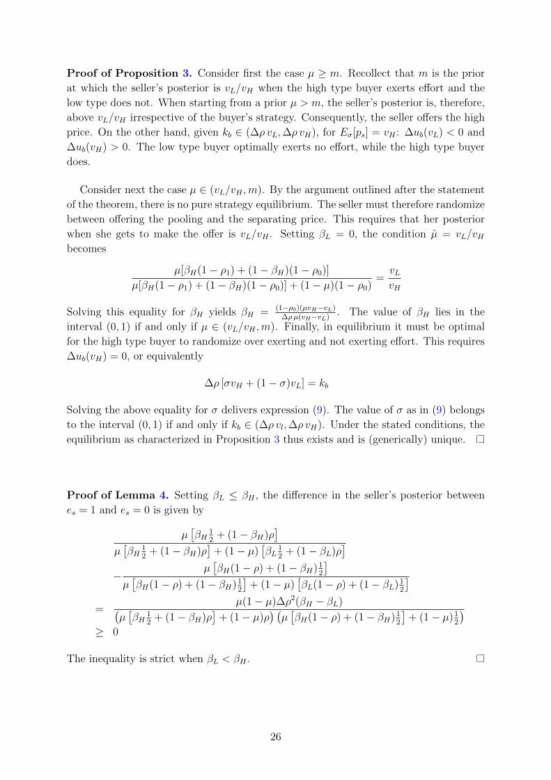
Proof of Proposition 3. Consider first the case µ ≥ m. Recollect that m is the prior
at which the seller’s posterior is vL/vH when the high type buyer exerts effort and the
low type does not. When starting from a prior µ > m, the seller’s posterior is, therefore,
above vL/vH irrespective of the buyer’s strategy. Consequently, the seller offers the high
price. On the other hand, given kb ∈ (∆ρ vL,∆ρ vH), for Eσ[ps] = vH : ∆ub(vL) < 0 and
∆ub(vH) > 0. The low type buyer optimally exerts no effort, while the high type buyer
does.
Consider next the case µ ∈ (vL/vH ,m). By the argument outlined after the statement
of the theorem, there is no pure strategy equilibrium. The seller must therefore randomize
between offering the pooling and the separating price. This requires that her posterior
when she gets to make the offer is vL/vH . Setting βL = 0, the condition µ = vL/vHbecomes
µ[βH(1− ρ1) + (1− βH)(1− ρ0)]
µ[βH(1− ρ1) + (1− βH)(1− ρ0)] + (1− µ)(1− ρ0)=vLvH
Solving this equality for βH yields βH = (1−ρ0)(µvH−vL)∆ρµ(vH−vL)
. The value of βH lies in the
interval (0, 1) if and only if µ ∈ (vL/vH ,m). Finally, in equilibrium it must be optimal
for the high type buyer to randomize over exerting and not exerting effort. This requires
∆ub(vH) = 0, or equivalently
∆ρ [σvH + (1− σ)vL] = kb
Solving the above equality for σ delivers expression (9). The value of σ as in (9) belongs
to the interval (0, 1) if and only if kb ∈ (∆ρ vl,∆ρ vH). Under the stated conditions, the
equilibrium as characterized in Proposition 3 thus exists and is (generically) unique.
Proof of Lemma 4. Setting βL ≤ βH , the difference in the seller’s posterior between
es = 1 and es = 0 is given by
µ[βH
12
+ (1− βH)ρ]
µ[βH
12
+ (1− βH)ρ]
+ (1− µ)[βL
12
+ (1− βL)ρ]
−µ[βH(1− ρ) + (1− βH)1
2
]µ[βH(1− ρ) + (1− βH)1
2
]+ (1− µ)
[βL(1− ρ) + (1− βL)1
2
]=
µ(1− µ)∆ρ2(βH − βL)(µ[βH
12
+ (1− βH)ρ]
+ (1− µ)ρ) (µ[βH(1− ρ) + (1− βH)1
2
]+ (1− µ)1
2
)≥ 0
The inequality is strict when βL < βH .
26
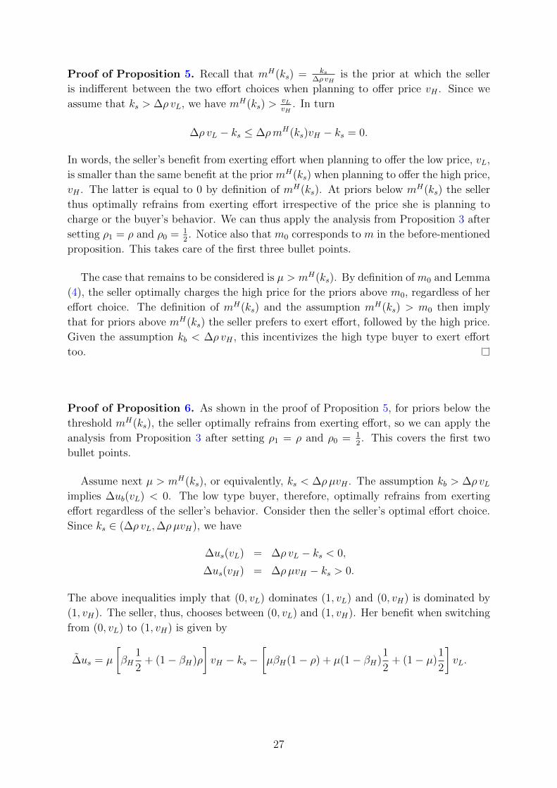
Proof of Proposition 5. Recall that mH(ks) = ks∆ρ vH
is the prior at which the seller
is indifferent between the two effort choices when planning to offer price vH . Since we
assume that ks > ∆ρ vL, we have mH(ks) >vLvH
. In turn
∆ρ vL − ks ≤ ∆ρmH(ks)vH − ks = 0.
In words, the seller’s benefit from exerting effort when planning to offer the low price, vL,
is smaller than the same benefit at the prior mH(ks) when planning to offer the high price,
vH . The latter is equal to 0 by definition of mH(ks). At priors below mH(ks) the seller
thus optimally refrains from exerting effort irrespective of the price she is planning to
charge or the buyer’s behavior. We can thus apply the analysis from Proposition 3 after
setting ρ1 = ρ and ρ0 = 12. Notice also that m0 corresponds to m in the before-mentioned
proposition. This takes care of the first three bullet points.
The case that remains to be considered is µ > mH(ks). By definition of m0 and Lemma
(4), the seller optimally charges the high price for the priors above m0, regardless of her
effort choice. The definition of mH(ks) and the assumption mH(ks) > m0 then imply
that for priors above mH(ks) the seller prefers to exert effort, followed by the high price.
Given the assumption kb < ∆ρ vH , this incentivizes the high type buyer to exert effort
too.
Proof of Proposition 6. As shown in the proof of Proposition 5, for priors below the
threshold mH(ks), the seller optimally refrains from exerting effort, so we can apply the
analysis from Proposition 3 after setting ρ1 = ρ and ρ0 = 12. This covers the first two
bullet points.
Assume next µ > mH(ks), or equivalently, ks < ∆ρ µvH . The assumption kb > ∆ρ vLimplies ∆ub(vL) < 0. The low type buyer, therefore, optimally refrains from exerting
effort regardless of the seller’s behavior. Consider then the seller’s optimal effort choice.
Since ks ∈ (∆ρ vL,∆ρ µvH), we have
∆us(vL) = ∆ρ vL − ks < 0,
∆us(vH) = ∆ρ µvH − ks > 0.
The above inequalities imply that (0, vL) dominates (1, vL) and (0, vH) is dominated by
(1, vH). The seller, thus, chooses between (0, vL) and (1, vH). Her benefit when switching
from (0, vL) to (1, vH) is given by
∆us = µ
[βH
1
2+ (1− βH)ρ
]vH − ks −
[µβH(1− ρ) + µ(1− βH)
1
2+ (1− µ)
1
2
]vL.
27
This term is decreasing in βH and equal to zero when βH takes the value
βH =12(vH − vL) + ∆ρ µvH − ks
∆ρ µ(vH − vL). (8)
We next argue that in equilibrium the seller cannot choose (0, vL) with probability one.
Recalling the assumption kb > ∆ρ vL, if the seller would choose (0, vL) with probability
one, the high type buyer would prefer not to exert effort:
∆ub(vH) = ∆ρ vL − kb < 0.
We would thus have βH = 0 and hence
∆us = µρvH − ks − 1/2vL,
> µρvH − ks − 1/2µvH ,
= ∆ρ µvH − ks,> 0,
where the first inequality follows from the assumption µvH > vL and the second from
ks < ∆ρ µvH . By implication, the seller would find it optimal to deviate to (1, vH).
Consider next the possibility of an equilibrium where the seller chooses (1, vH) with
probability one. This makes it optimal for the high type buyer to exert effort:
∆ub(vH) = ∆ρ vH − kb > 0,
where the inequality follows from the assumption kb < ∆ρ vH . Given βH = 1, we then
have
∆us =1
2(µvH − vL) + ∆ρ µvL − ks.
For (1, vH) to be optimal, the above term needs to be non-negative. This is the case if
µ ≥ks + 1
2vL
12vH + ∆ρ vL︸ ︷︷ ︸
=m(ks)
.
Hence, when µ ≥ m(ks), there exists a pure strategy equilibrium where the seller and the
high type buyer exert effort, while the low type does not, and the seller offers price vH .
When the above inequality is not satisfied, the seller must randomize between (0, vL)
and (1, vH) in equilibrium. Indifference between the two tuples requires ∆us = 0. As we
showed above, this condition is satisfied if βH takes the value in (8). Given the assumption
µ > mH(ks), this value of βH lies in (0, 1) if and only if µ < m(ks). Finally, randomizing
28
is optimal for the high type buyer if
∆ub(vH) = ∆ρ [σvH + (1− σ)vL]− kb = 0.
Solving the equality for σ yields
σ =kb −∆ρ vL
∆ρ (vH − vL). (9)
It can be verified that under the imposed parameter restrictions, the above term lies in
(0, 1).
Taken together, this shows that the equilibrium, as described in Proposition 6, exists
and that it is unique.
Proof of Proposition 7. If the seller gets to make an offer, her posterior belief about
the buyer’s type is
µ =µ(1− ρH)
µ(1− ρH) + (1− µ)(1− ρL).
She optimally offers price vH if her posterior belief exceeds vL/vH , i.e. if
µ(1− ρH)
µ(1− ρH) + (1− µ)(1− ρL)≥ vL/vH .
Solving this inequality for µ, yields expression (7).
References
Board, S. and J. Zwiebel (2012): “Endogenous competitive bargaining,” Tech. rep.,
mimeo.
Cialdini, R. B. and N. Garde (1987): Influence, vol. 3, A. Michel.
Evans, R. (1997): “Coalitional bargaining with competition to make offers,” Games and
Economic Behavior, 19, 211–220.
Fisher, R., W. L. Ury, and B. Patton (2011): Getting to yes: Negotiating agreement
without giving in, Penguin.
Fudenberg, D. and J. Tirole (1983): “Sequential bargaining with incomplete infor-
mation,” The Review of Economic Studies, 50, 221–247.
——— (1991): “Game theory, 1991,” Cambridge, Massachusetts, 393, 12.
29
Grennan, M. (2014): “Bargaining ability and competitive advantage: Empirical evi-
dence from medical devices,” Management Science, 60, 3011–3025.
Gul, F., H. Sonnenschein, and R. Wilson (1986): “Foundations of dynamic
monopoly and the Coase conjecture,” Journal of Economic Theory, 39, 155–190.
Heinsalu, S. (2017): “Investing to Access an Adverse Selection Market,” .
Inderst, R. (2001): “Screening in a matching market,” The Review of Economic Studies,
68, 849–868.
Krasteva, S. and H. Yildirim (2012): “Payoff uncertainty, bargaining power, and
the strategic sequencing of bilateral negotiations,” The RAND Journal of Economics,
43, 514–536.
Merlo, A. and C. Wilson (1995): “A stochastic model of sequential bargaining with
complete information,” Econometrica: Journal of the Econometric Society, 371–399.
Munster, J. and M. Reisinger (2015): “Sequencing bilateral negotiations with ex-
ternalities,” .
Okada, A. (1996): “A noncooperative coalitional bargaining game with random pro-
posers,” Games and Economic Behavior, 16, 97–108.
Rubinstein, A. (1982): “Perfect equilibrium in a bargaining model,” Econometrica:
Journal of the Econometric Society, 97–109.
Rubinstein, A. and A. Wolinsky (1985): “Equilibrium in a market with sequential
bargaining,” Econometrica: Journal of the Econometric Society, 1133–1150.
Stahl, I. (1972): “Bargaining Theory (Stockholm School of Economics),” Stockholm,
Sweden.
Trump, D. J. and T. Schwartz (2009): Trump: The art of the deal, Ballantine Books.
Yildirim, H. (2007): “Proposal power and majority rule in multilateral bargaining with
costly recognition,” Journal of Economic Theory, 136, 167–196.
——— (2010): “Distribution of surplus in sequential bargaining with endogenous recog-
nition,” Public choice, 142, 41.
Zingales, L. (1995): “Insider ownership and the decision to go public,” The Review of
Economic Studies, 62, 425–448.
30