Investigations Osc

8/8/2019 Investigations Osc

http://slidepdf.com/reader/full/investigations-osc 1/26

15913074 Page 1

Student number 15913074

Rebecca Rollins



15913074 P 2

Contents Page

Page 3 ± Summary

Page 4 ± Introduction

Page 5 ± No damping or dr iving force

Page 9 ± Accuracy of numer ical solutions

Page 10 ± Damping, no dr iving force

Page 16 ± Dr iving force, no damping

Page 18 ± Damped, dr iven oscillator

Page 19 ± Chaos

Page 20 ± Poincare maps

Page 23 - Extensions

Page 24 ± Conclusion

Page 25 ± Acknowledgements

Page 26 - Appendices



15913074 P 3

Summary

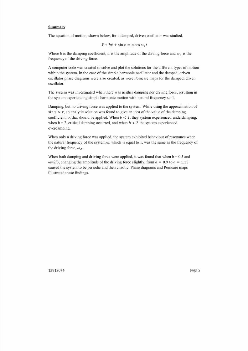
The equation of motion, shown below, for a damped, dr iven oscillator was studied.

Where b is the damping coeff icient, is the amplitude of the dr iving force and is thefrequency of the dr iving force.

A computer code was created to solve and plot the solutions for the different types of motion

within the system. In the case of the simple harmonic oscillator and the damped, dr iven

oscillator phase diagrams were also created, as were Poincare maps for the damped, dr iven

oscillator.

The system was investigated when there was neither damping nor dr iving force, resulting in

the system exper iencing simple harmonic motion with natural frequency=1.

Damping, but no dr iving force was applied to the system. While using the approximation of

, an analytic solution was found to give an idea of the value of the damping

coeff icient, b, that should be applied. When , they system exper ienced underdamping,

when b = 2, cr itical damping occurred, and when the system exper ienced

overdamping.

When only a dr iving force was applied, the system exhi bited behaviour of resonance when

the natural frequency of the system, which is equal to 1, was the same as the frequency of

the dr iving force, .

When both damping and dr iving force were applied, it was found that when b = 0.5 and

=2/3, changing the amplitude of the dr iving force slightly, from

to

caused the system to be per iodic and then chaotic. Phase diagrams and Poincare maps

illustrated these f indings.



15913074 P 4

Introduction

Whether it is a grandfather clock behaving with simple harmonic motion, or a damped system

providing shock absorbers for cars, the types of motion a par ticular system exhi bits can be

extremely interesting and relevant to real life.

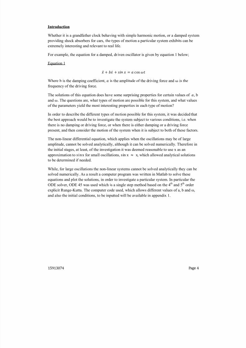
For example, the equation for a damped, dr iven oscillator is given by equation 1 below;

Equation 1

Where b is the damping coeff icient, is the amplitude of the dr iving force and is the

frequency of the dr iving force.

The solutions of this equation does have some surpr ising proper ties for cer tain values of , b

and . The questions are, what types of motion are possi ble for this system, and what values

of the parameters yield the most interesting proper ties in each type of motion?

In order to descr i be the different types of motion possi ble for this system, it was decided that

the best approach would be to investigate the system subject to var ious conditions, i.e. when

there is no damping or dr iving force, or when there is either damping or a dr iving force

present, and then consider the motion of the system when it is subject to both of these factors.

The non-linear differential equation, which applies when the oscillations may be of large

amplitude, cannot be solved analytically, although it can be solved numer ically. Therefore in

the initial stages, at least, of the investigation it was deemed reasonable to use x as an

approximation to

for small oscillations,

which allowed analytical solutions

to be determined if needed.

While, for large oscillations the non-linear systems cannot be solved analytically they can be

solved numer ically. As a result a computer program was wr itten in Matlab to solve these

equations and plot the solutions, in order to investigate a par ticular system. In par ticular the

ODE solver, ODE 45 was used which is a single step method based on the 4th

and 5th

order

explicit R unge-Kutta. The computer code used, which allows different values of a, b and ,

and also the initial conditions, to be inputted will be available in appendix 1.



15913074 P 5

No damping or driving force

Small oscillations

The most well known, and simplest, type of motion for this system occurs when both

damping and dr iving force are absent. This results in the following equation of motion;

Equation 2

This par ticular equation descr i bes simple harmonic motion, which is motion that behaves in

a per iodic fashion, repeating itself in a sinusoidal manner with constant amplitude. (The

natural frequency of the system is=1.)

This equation is known to have the following solution;

Equation 3

Equation 4 = Where A, B and C are constants, is the angular frequency, in this case =1, is the

amplitude, (+) is the phase at time t and is the initial phase. The amplitude and phase

are determined by the initial conditions of the system i.e. position and velocity.

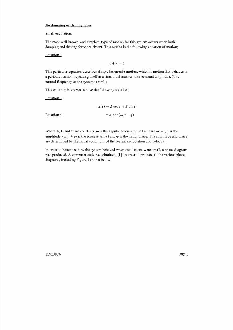
In order to better see how the system behaved when oscillations were small, a phase diagram

was produced. A computer code was obtained, [1], in order to produce all the var ious phasediagrams, including Figure 1 shown below.



15913074 P 6

Figure 1 A phase diagram for the simple harmonic oscillator. The trajector ies are indicated in

blue, while the red arrows show the direction the points move with time in the phase space.

The concentr ic circles show the constant per iodic motion of the oscillator for small

oscillations, resulting from the absence of a damping and dr iving force.

-6 -5 -4 -3 -2 -1 0 1 2 3 4 5 6-6

-5

-4

-3

-2

-1

0

1

2

3

4

5

6

displacement

a n g u l a r v e l o c i t y



15913074 P 7

-6 -5 -4 -3 -2 -1 0 1 2 3 4 5 6-6-5

-4

-3

-2

-1

0

1

2

3

45

6

displacement

a n g u l a r

e l o c i t y

Large Oscillations

Having studied the system with small oscillations, i.e. , a natural progression was to

study what effect using large oscillations in the system would produce. In this case the

equation of motion studied is given by;

Equation 5

As stated previously, the numer ical solution to this equation was obtained from the computer

code and plotted. Many graphs were produced, using var ious initial conditions. However,

ultimately a phase diagram was used. This allowed for a clearer picture of the behaviour of

the system to be seen, and more impor tantly, a compar ison could be made with Figure 1 to

show what effects there would be for large oscillations.

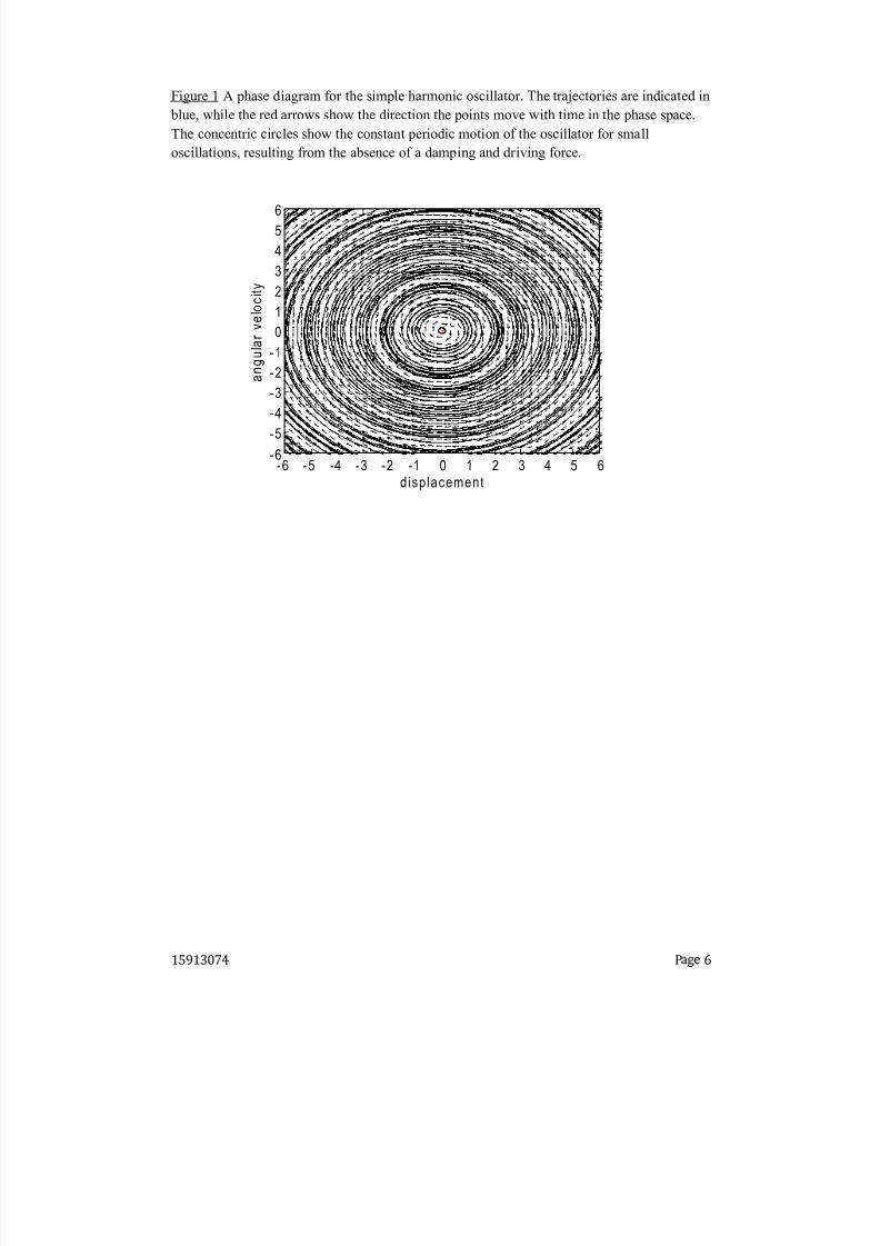
The phase diagram for large oscillations is shown below in f igure 2;

Figure 2 A phase diagram for large oscillations when a damping and dr iving force are absent.

The trajector ies are indicated in blue, while the red arrows show the direction the points move

with time in the phase space. Several stationary points can be seen on the phase diagram.

Saddle points can be seen at , n. Elli ptical f ixed points can be seen at , n



15913074 P 8

A saddle point, also known as a hyperbolic f ixed point, is a point in the domain of

a function which is a stationary point but not a local extremum. In terms of contour lines, a

saddle point can be recognized, in general, by a contour that appears to intersect itself [2]. A

saddle point has eigenvalues, .

In this case, the eigenvalues are

.

An elliptical fixed point of a differential equation is a f ixed point for which the Jacobian has

purely imaginary eigenvalues, [3]

In this case, the eigenvalues are .These eigenvalues were determined by using the Jacobian given by equation 6, [4];

Equation 6

Given a set of n equations in n var iables,

, the Jacobian matr ix is def ined

as;

This equation was adapted to f ind the eigenvalues for equation 5, resulting in the

identif ication of the saddle and elli ptical f ixed points. The full method used for this equation

can be found in appendix 2.

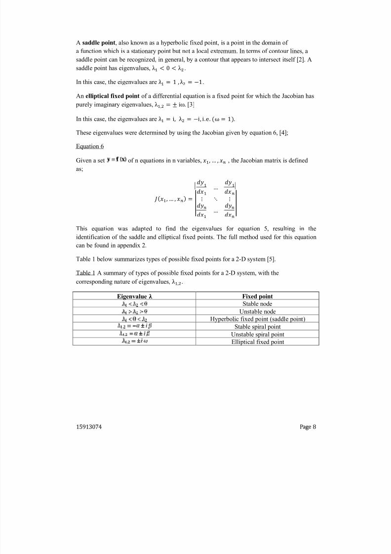
Table 1 below summar izes types of possi ble f ixed points for a 2-D system [5].

Table 1 A summary of types of possi ble f ixed points for a 2-D system, with the

corresponding nature of eigenvalues, .Eigenvalue Fixed point

Stable node

Unstable node

Hyperbolic f ixed point (saddle point)

Stable spiral point

Unstable spiral point

Elli ptical f ixed point



15913074 P 9

0 5 1 0 1 5 2 0 2 5 30 3 5 4 0 4 5 50-0. 01

-0. 008

-0. 006

-0. 004

-0. 002

0

0 . 0 0 2

0 . 0 0 4

0 . 0 0 6

0 . 0 0 8

0. 01

Ti ¡ ¢

D i

£

¤

l¥

¦

§

¨

§

©

A

h

h wi

h ¢

l i

l

!

" ¡ ¢ i

l

l " i

f h ¢

i ¡ l ¢ h ¡

i

il l

l

i

" ¡ ¢

i

l

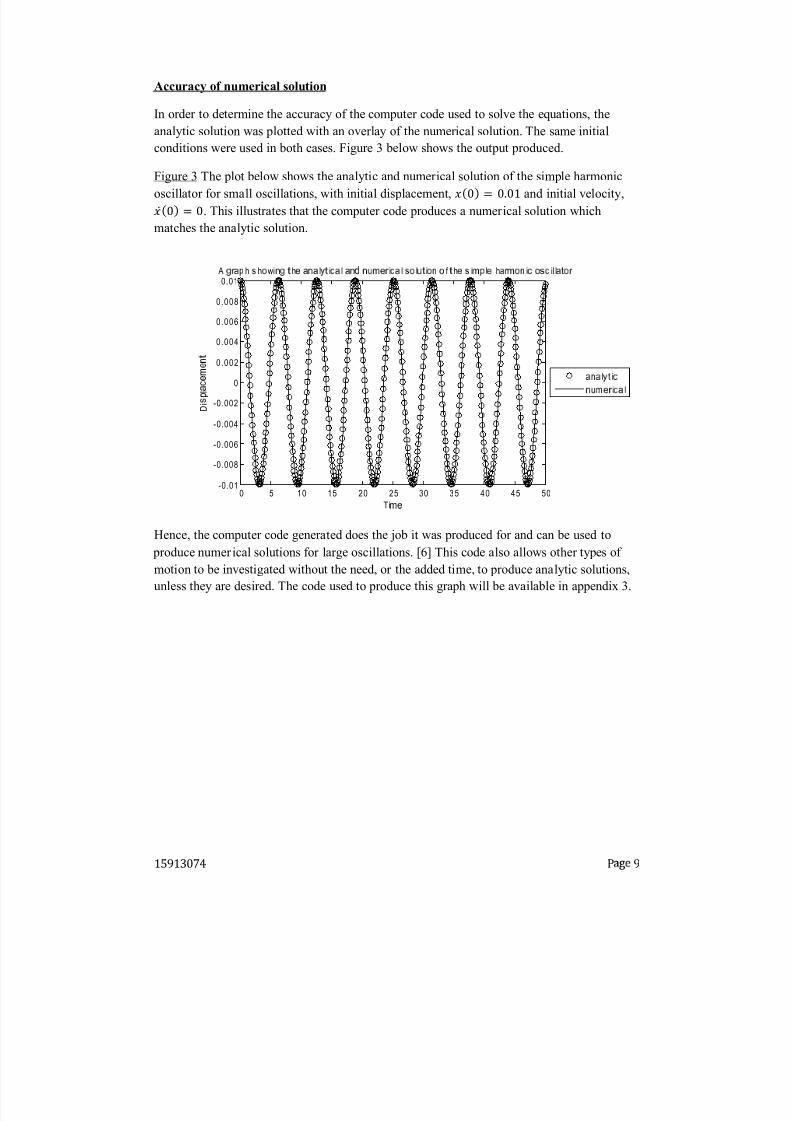
Accuracy of numerical solution

In order to determine the accuracy of the computer code used to solve the equations, the

analytic solution was plotted with an over lay of the numer ical solution. The same initial

conditions were used in both cases. Figure 3 below shows the out put produced.

Figure 3 The plot below shows the analytic and numer ical solution of the simple harmonicoscillator for small oscillations, with initial displacement, and initial velocity, . This illustrates that the computer code produces a numer ical solution which

matches the analytic solution.

Hence, the computer code generated does the job it was produced for and can be used to

produce numer ical solutions for large oscillations. [6] This code also allows other types of

motion to be investigated without the need, or the added time, to produce analytic solutions,

unless they are desired. The code used to produce this graph will be available in appendix 3.



15913074 P 10

Damping, no driving force

In any real life situation an oscillator will be subject to the effects of damping, most

commonly fr iction or air resistance. Under this damping force it is to be expected that free

oscillations will decrease with time i.e. the amplitude of the oscillations will gradually be

reduced as energy in the system is slowly dissi pating. The question remains, what value of b

will allow the system to return to its equili br ium position in the quickest time?

The equation of the system that was studied is given by equation 7 below;

Equation 7

The computer program was used to produce var ious out puts for different values of b for both

small and large oscillations. With the same approximate results, it was decided that the

equation of motion for small oscillations would be solved analytically to give an indication of

the values of b that would produce the most interesting results.

For small oscillations equation 7 becomes equation 8, as shown below;

Equation 8

Where b is the damping coeff icient.

Initially the computer program was used to solve equation 8 and plot the solution using

var ious values of b, ranging from b=0.5 to b=0.025. The graphs showed that, as expected, as

the dampening increased the time taken for the system to return to equili br ium decreased,until b=0 and the system once again exhi bits simple harmonic motion.

It was also shown that unlike in strongly damped systems, the oscillations continue to persist

in weak ly damped system.

Figure 4 (a), (b) and (c) below highlight some of the results found.



15913074 P 11

0 20 40 60 80 100 120 140 160 180 200-6

-4

-2

0

2

4

6

8

10

12

14x 10

-3

0 20 40 60 80 100 120 140 160 180 200-0.015

-0.01

-0.005

0

0.005

0.01

0.015

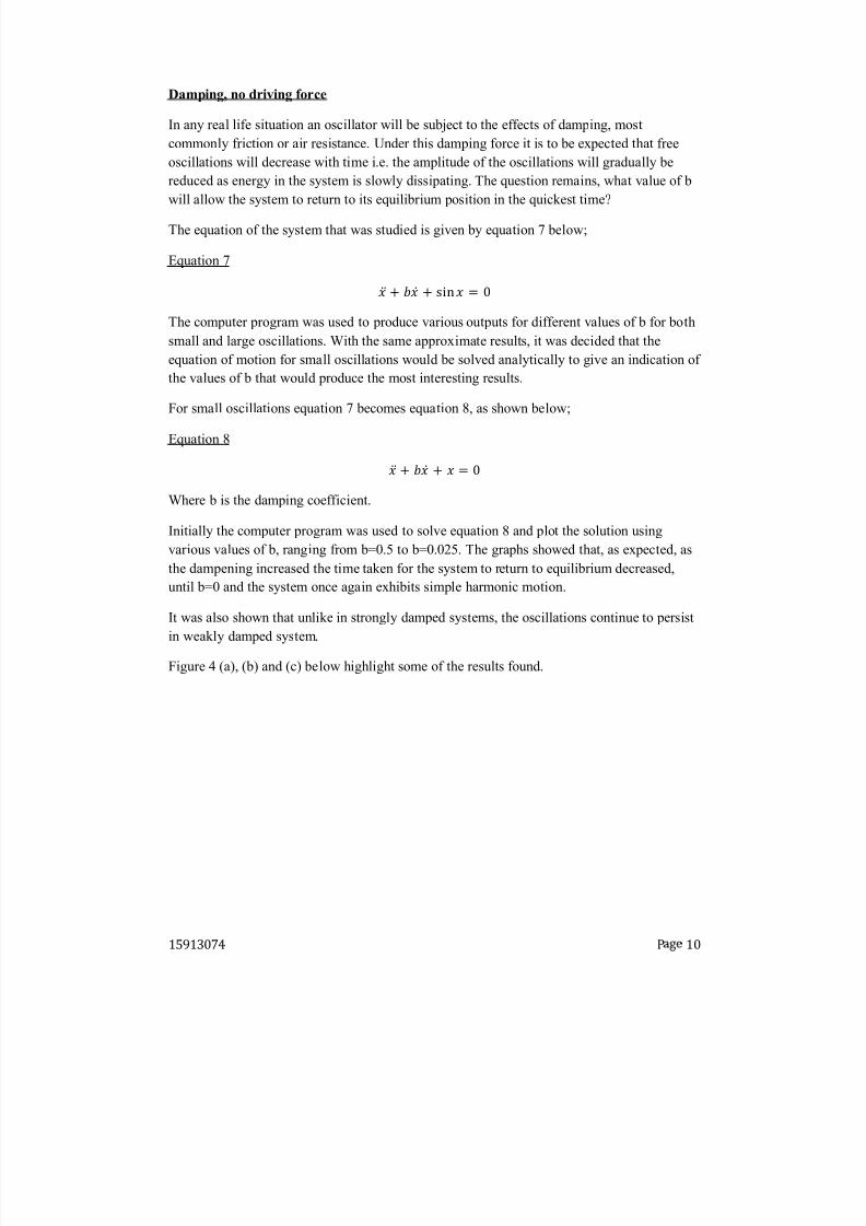
Figure 4

(a) Solution for strong damping with b=0.5, initial conditions .

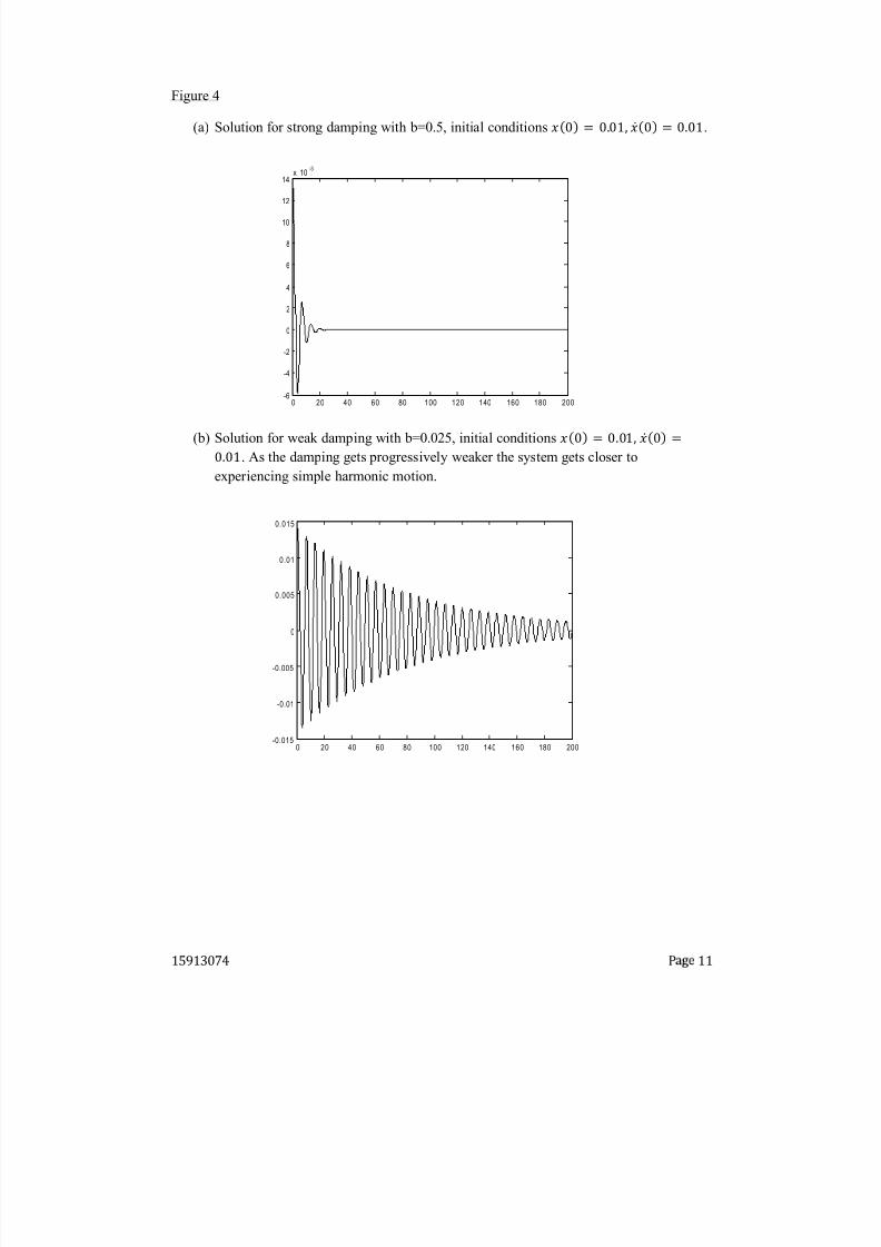
(b) Solution for weak damping with b=0.025, initial conditions . As the damping gets progressively weaker the system gets closer to

exper iencing simple harmonic motion.



15913074 P 12

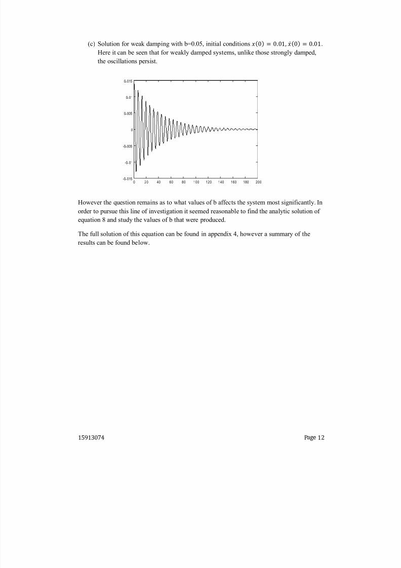
(c) Solution for weak damping with b=0.05, initial conditions .

Here it can be seen that for weak ly damped systems, unlike those strongly damped,

the oscillations persist.

However the question remains as to what values of b affects the system most signif icantly. In

order to pursue this line of investigation it seemed reasonable to f ind the analytic solution of

equation 8 and study the values of b that were produced.

The full solution of this equation can be found in appendix 4, however a summary of the

results can be found below.

0 20 40 60 80 100 120 140 160 180 200-0 015

-0 01

-0 005

0

0 005

0 01

0 015



15913074 Page 13

0 5 10 15 20 25 30 35 40 45 50-4

-2

0

2

4

6

8x 10

-3 b = 0 . 5 [0,0.01]

Equation 9

Auxiliary Equation

Equation 10

(a)

(b)

(c) General solution,

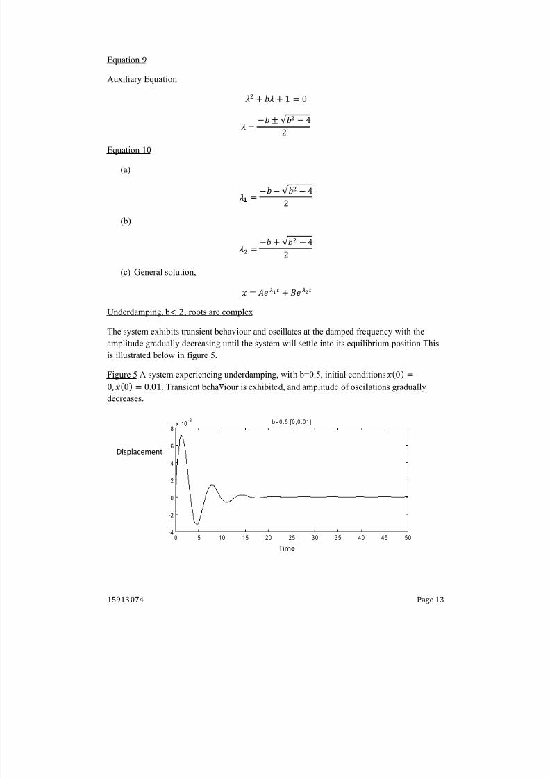
Underdamping, b , roots are complex

The system exhibits transient beha iour and oscillates at the damped frequency with the

amplitude gradually decreasing until the system will settle into its equilibrium position. This

is illustrated below in figure 5.

Figure 5 A system experiencing underdamping, with b=0.5, initial conditions . Transient beha iour is exhibited, and amplitude of oscillations gradually

decreases.

Time

Displacement



15913074 Page 14

0 5 10 15 20 25 30 35 40 45 50-2

0

2

4

6

8

10

12

14x 10

-3

0 5 10 15 20 25 30 35 40 45 50-2

0

2

4

6

8

10

12x 10

-3

Disp lacement

T i m

e

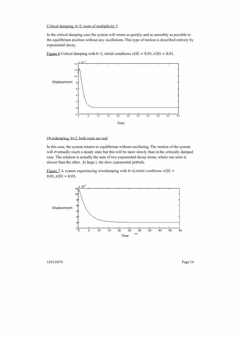
Critical damping, b=2, roots of multiplicity 2

In the critical damping case the system will return asquickly and as smoothly as possible to

the equilibrium position without any oscillations. This type of motion is described entirely by

exponential decay.

Figure 6 Critical damping with b=2, initial conditions .

O erdamping, b2, both roots are real

In this case, the system returns to equilibrium without oscillating. The motion of the system

will e entually reach a steady state but this will be more slowly than in the critically damped

case. The solution is actually the sum of two exponential decay terms, where one term is

slower than the other. At large t, the slow exponential pre ails.

Figure 7 A system experiencing o erdamping with b=4, initial conditions .

Displacement

Time

Time

Displacement



15913074 Page 15

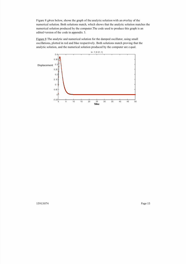
Figure 8 gi en below, shows the graph of the analytic solution with an o erlay of the

numerical solution. Both solutions match, which shows that the analytic solution matches the

numerical solution produced by the computer.The code used to produce this graph is an

edited ersion of the code in appendix 3.

Figure 8 The analytic and numerical solution for the damped oscillator, using small

oscillations, plotted in red and blue respecti ely. Both solutions match pro ing that the

analytic solution, and the numerical solution produced by the computer are equal.

Time

Displacement

0 5 10 15 20 25 30 35 40 45 50-0 .0 5

0

0 .05

0 .1

0 .15

0 .2

0 .25

0 .3

0 .35

0 .4

$

i% e

b= 2 [0 .01,1 ]



15913074 P 16

Driving force , no damping

Having investigated the implications of applying a damping force to the system it seemed like

a sensi ble idea to also investigate the type of motion produced when a dr iving force is

applied. A dr iving force is used to feed energy into the system.Therefore the equation of

motion to be studied is given by equation 11 below;

Equation 11

Where is the dr iving frequency, and is the amplitude of the dr iving force in this case.

As with other previous systems, equation 11 was investigated for both small oscillations i.e. , and large oscillations. In each case var ious values for and were investigated

using a range of initial conditions.

However, in both cases for small and large oscillations, a par ticular ly interesting result

occurred when .

To illustrate this result, a dr iving force was applied to the simple harmonic oscillator resulting

in equation 12 below.

Equation 12

The condition when the dr iving frequency is equal to the natural frequency of the system,

R esonance is the increase in the amplitude of an oscillation of a system, under the inf luence

of a per iodic force whose frequency is close to that of the system's natural frequency [7]. This

is illustrated in f igure 10 below.



15913074 Page 17

0 2 0 4 0 6 0 8 0 1 0 0 1 2 0 1 4 0 1 6 0 1 8 0 2 0 0-10 0

-80

-60

-40

-20

0

20

40

60

80

10 0

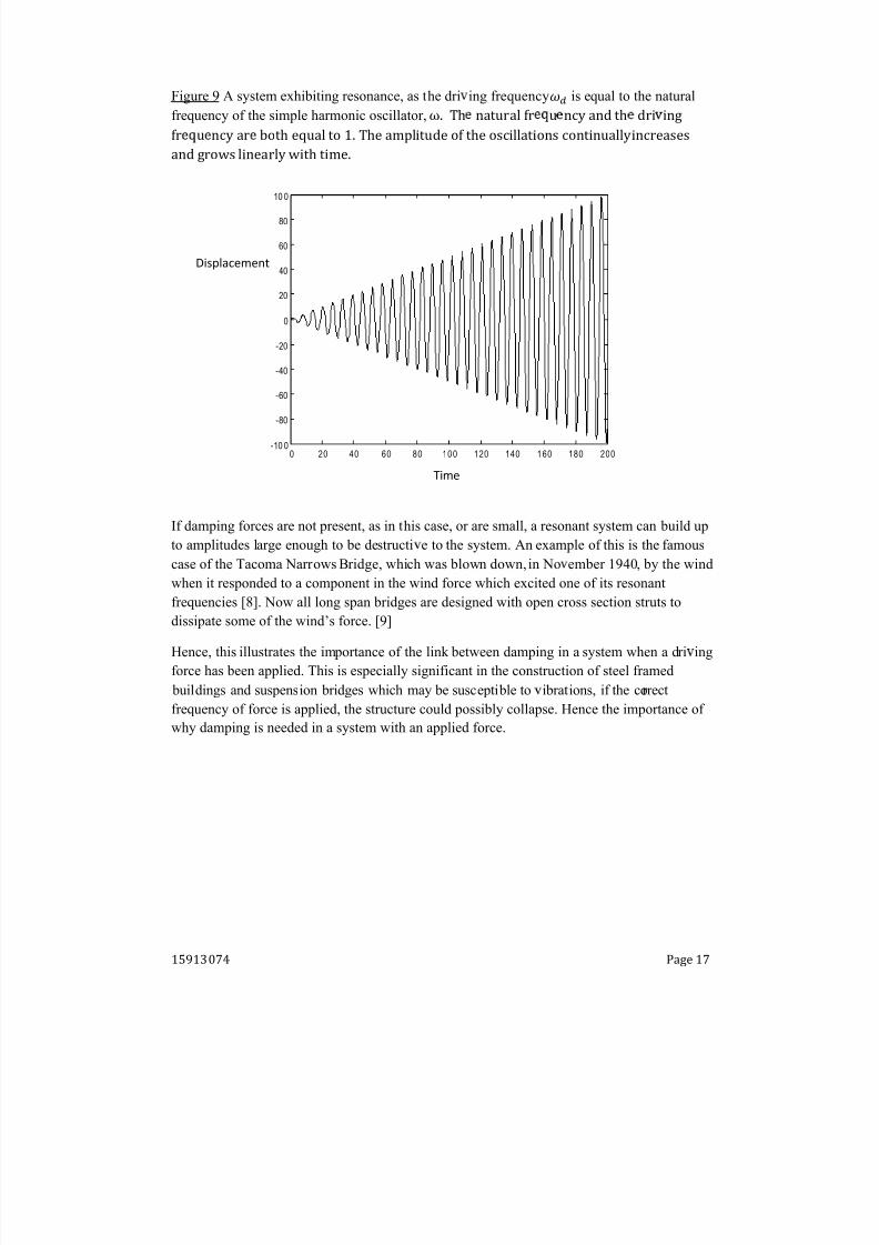
Figure 9 A system exhibiting resonance, as the dri ing frequency is equal to the natural

frequency of the simple harmonic oscillator,

If damping forces are not present, as in this case, or are small, a resonant system can build up

to amplitudes large enough to be destructi e to the system. An example of this is the famous

case of the Tacoma Narrows Bridge, which was blown down, in No ember 1940, by the wind

when it responded to a component in the wind force which excited one of its resonantfrequencies [8]. Now all long span bridges are designed with open cross section struts to

dissipate some of the wind¶s force. [9]

Hence, this illustrates the importance of the link between damping in a system when a dri ing

force has been applied. This is especially significant in the construction of steel framed

buildings and suspension bridges which may be susceptible to ibrations, if the correct

frequency of force is applied, the structure could possibly collapse. Hence the importance of

why damping is needed in a system with an applied force.

Time

Displacement



15913074 P 18

Damped, Driven Oscillator

Since the var ious types of motion within the system have been investigated, an appropr iate

progression was to investigate the system in its entirety with both damping and a dr iving

force applied.

The system to be investigated was given by equation 1, and is also shown below. Where b is the damping coeff icient, amplitude of dr iving force and is the dr iving

frequency.

The solution to equation of motion above is made up of two par ts, the transient and steady

state par t. The transient par t is the solution to the damping equation. A dr iven system will

ultimately settle down to a behaviour that is determined by the steady state par t of the

solution. Since the effects of the transient solution will ultimately die out, it seemed a natural

A sensi ble star ting point was to use the computer program to investigate the solution of the

above equation, using var ious values of , b and . This resulted in some interesting

obser vations. In this case the computer code was edited to produce phase diagrams, which

better showed the behaviour of the var ious results produced. The edited version of the

computer code used can be found in appendix 5.

It was found that if values b = 0.5 and were set for the system, and a small dr iving

amplitude, was applied, then once the transient effects had died out, the system

would exhi bit per iodic behaviour. This per iodic behaviour is due to the steady state par t of

the equation.

The dr iving amplitude was slightly increased to , and once transient effects died out,

the system exhi bited double per iodic behaviour.

Once again the dr iving amplitude was increased slightly to and af ter transient

effects had died out the system exhi bited chaotic behaviour.

This change in behaviour is resultant in only a slight change of dr iving amplitude suggesting

that this system is sensitive to initial conditions.



15913074 P 19

Chaos

Although there is no def initive, universal def inition of chaos, a commonly used def inition

states that the following proper ties must be satisf ied for a dynamical system to be classif ied

as µchaotic¶. [10]

1. The system must be sensitive to initial conditions,2. It must be topologically mixing,

3. Its per iodic orbits must be dense.

The ³Butterf ly Effect´ is a common metaphor used to emphasise the concept that the system

is sensitive to the initial conditions enforced. ³Does the f lap of a butterf ly¶s wings set in

Brazil set off a tornado in Texas?´ - Phili p Mer ilees [11]. The phrase refers to the idea that the f lap of a butterf ly¶s wings can create tiny changes in the

atmosphere; changes which could alter the path or acceleration of a tornado, i.e. a small

change in the initial conditions can have a signif icant knock on effect to the behaviour of the

system.

Table 2 shows the character istics and behaviour of the system for var ious values of the

amplitude of the dr iving force, [12]

Table 2 Behaviour of the system for a range of values of , when b = 0.5 and R ange Type of Behaviour Per iodic

Chaotic

Per iodic

Chaotic Per iodic Chaotic Per iodic Chaotic Per iodic Chaotic Per iodic Chaotic



15913074 P 20

-3 -2 -1 0 1 2 3-2

-1

0

1

2

3

& isp lace'

en(

)

n g u l a r V e l o c i

0

y

1 p2

a s e d ia gr a'

s2

o3

i ng p er o di c b e2

aviou r o 4 a s ys(

e'

3

2

en a= 0 .9 , b= 0 .5 a nd3

= 2/ 3

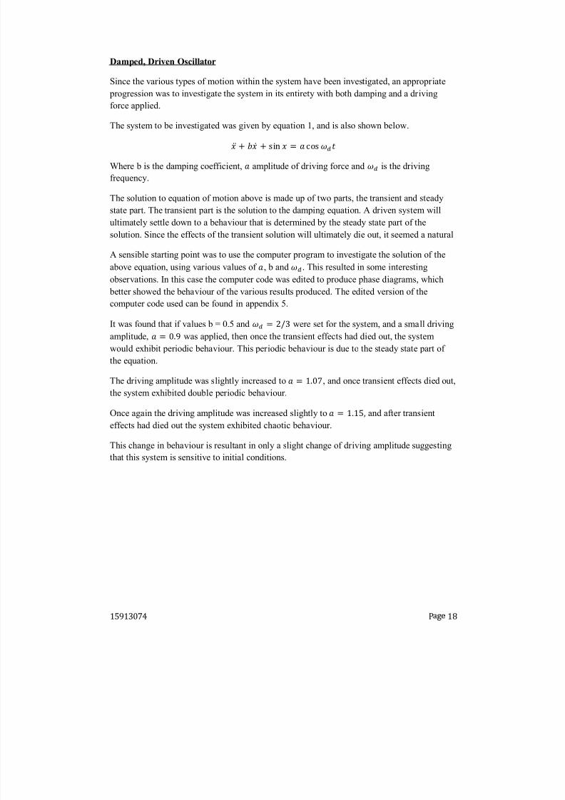
Figure 10 (a) and (b) show the phase diagrams for per iodic and chaotic behaviour. (For the

purposes of the titles only in f igure 11 (a) and (b), is represented by w.)

Figure 10

(a) The transient effects can be seen in the phase diagram but as these effects die off, the

system exhi bits per iodic behaviour, when b = 0.5, and .

(b) A chaotic system will encompass the entire phase space and unlike per iodic

behaviour it will not be contained to a single, or even double, loop. The system shown

is chaotic when when b = 0.5, and .

-4 -3 -2 -1 0 1 2 3 4-3

-2

-1

0

1

2

3

D i5

6

l7

8 9

@

9 A

B

A

C

D

E

lF

G

V

H

lI

P

iQ

R

A ph7

5 9

d i7

S

T 7 @

s hU V

iA S

a sys tem eW

h iX

itiA S

c hao t ic be haviour w ith a= 1 .15 , b= 0.5 and w= 2/ 3



15913074 P 21

-Y

.5Y Y

.5`

.5Y

Y .5

.5

D ia

b

lc d e

me f

t

A

g

g

h

li

r V

p

l

q

r

i ts

P t

if d c r e a e d t i t f t f c a u a t e

m e x h iv

it i f gb

e r i t w

id v e h c x

it y r

Poincare Map

A Poincare map, (also known as a Poincare section) or f irst return map of solutions in which

the frequency of the dr iving force, , is known. The phase plan is still used however, only

the solutions at t = 0 and integer multi ples of

. In other words, a per iodic solution has a

Poincare map which is a single point on the plane. This is the f ixed point of the oscillation.

[13] Per iodic doubling will have Poincare map of two points on the plane etc.

Poincare maps were produced using a computer code to show per iodic, double per iodic and

chaotic behaviour in a system.This computer code can be found in appendix 6.

However, due to the sensitivity of the system to small initial changes, and the nature of the

default relative and absolute tolerance of the computer program, the Poincare maps contain

points due to error which would not naturally occur.

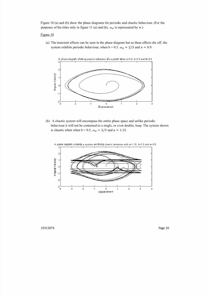
Figure 11

(a) The Poincare map for , when b = 0.5 and . The Poincare map for

per iodic behaviour should consist of a single point on the plane indicated by a heavier

shading of blue. However points that are due to errors do appear on the Poincare map.



15913074 P 22

-

.

-

.

5 -

.

-

.

5 -

.

-

.

5 -

.

.9

.9 5

.

5

is

l

c t

A

g

l

r V

l

c i t y

P

i

c

r

s

c t

i

s h

i

g

sy s t

x h i

it i

g

r i

ic

li

g

-

-

-

-

-

.5

.5

.5

.5

is

l

c

t

A

g

l

r V

l

c i t y

P

i

c

r

s

c ti

s h

i

g

s y s t

x hi

iti

g c h

t ic

h

vi

r

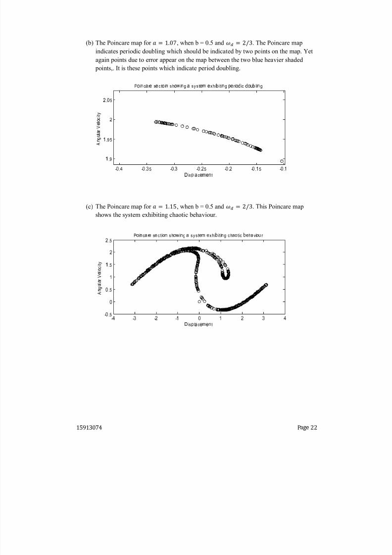
(b) The Poincare map for , when b = 0.5 and . The Poincare map

indicates per iodic doubling which should be indicated by two points on the map. Yet

again points due to error appear on the map between the two blue heavier shaded

points,. It is these points which indicate per iod doubling.

(c) The Poincare map for , when b = 0.5 and . This Poincare map

shows the system exhi biting chaotic behaviour.



15913074 P 23

Extensions

1. Due to the sensitivity of the system to initial conditions and the default values of the

relative and absolute error, when the Poincare maps were plotted, error points were

included in the plot. The relative and absolute tolerance could be adjusted for the

program by using the options=odeset command. Var ious values for the tolerances

could be tested until the suff icient values are obtained to produce the Poincare maps

without points caused by errors.

2. Since a slight change in the initial conditions, namely the value of frequency of the

dr iving force, can completely change the behaviour of a system from per iodic to

chaotic it may be useful to plot bifurcation diagrams. Bifurcation diagrams could be

produced by creating another computer code in Matlab. The Bifurcation Diagrams

allow for compar isons between the per iodic and chaotic behaviours of the system.



15913074 P 24

Conclusion

When neither damping nor dr iving force was applied to the system, the system exper ienced

simple harmonic motion with natural frequency=1.

When damping, but no dr iving force was applied to the system, and while using the

approximation of , the analytic solution produced the following results. When , they system exper ienced underdamping, when b = 2, cr itical damping occurred, and when the system exper ienced overdamping.

When only a dr iving force was applied, the system exhi bited behaviour of resonance when

the natural frequency of the system, which is equal to 1, was the same as the frequency of

the dr iving force, .

When both damping and dr iving force were applied, it was found that when b = 0.5 and=2/3, changing the amplitude of the dr iving force slightly, from to caused

the system to be per iodic and then chaotic respectively. This shows the sensitivity of the

system to changes in initial conditions. A range of values of were used from to . Phase diagrams and Poincare maps illustrated these f indings.



15913074 P 25

Ack nowledgements

I would like to acknowledge and thank Meredith Gr ieve for her time, patience and co-

operation provided to carry out this investigation; Dr H. Van der Har t and Dr G. Gr i bak in for

their guidance and hel p in producing the Matlab code needed for the investigation.

A list of fur ther resources used is given below;

[1] Lynch, Stephen. "Dynamical Systems with Applications using MATLAB".

Spr inger/Birkhauser, 2004.

[2] htt p://en.wik i pedia.org/wik i/Saddle_point, (23/02/10) [3] Weisstein, Er ic W. ³Elli ptic Fixed Point." From MathWorld --A Wolfram Web

R esource. htt p://mathwor ld.wolfram.com/Elli pticFixedPoint.html

[4] Weisstein, Er ic W. ³Jacobian." From MathWorld --A Wolfram Web

R esource. htt p://mathwor ld.wolfram.com/Jacobian.html

[5] Weisstein, Er ic W. ³Fixed Point." From MathWorld --A Wolfram Web

R esource. htt p://mathwor ld.wolfram.com/FixedPoint.html

[6] Fausett, Laurene V. ³Applied numer ical analysis using MATLAB´. Upper Saddle River,

NJ : London : Prentice Hall ; Prentice Hall International, c1999

[7] htt p://en.wik tionary.org/wik i/resonance, (25/02/10)

[8] htt p://hyperphys ics.phy-astr.gsu.edu/Hbase/oscdr2.html#c2 (23/02/10)

[9] htt p://hyper text book.com/chaos/41.shtml (22/02/10)

[10] htt p://en.wik i pedia.org/wik i/Chaos_ theory (26/02/10)

[11] htt p://en.wik i pedia.org/wik i/Chaos_ theory (26/02/10)

[12] Baker, Gregory L. Gollub, Jerry P. ³Chaotic Dynamics: an introduction . Cambr idge

University Press, NY; 1993.

[13] Smith, P. Smith, R .C. ³Mechanics´. John Wiley & Sons, 1990

Image on title page ± htt p://www.wor ldofstock.com/closeups/PR E9817.php (27/02/10)



Documents

Investigations Osc