Embed Size (px)
Citation preview

INVESTIGATION ON AN AIRBORNE MAGNETIC AND HELITEM
SURVEY ON FLIN FLON AREA
A Thesis Submitted to the College of
Graduate and Postdoctoral Studies
In Partial Fulfillment of the Requirements
For the Degree of Master of Science
In the Department of Geological Sciences
University of Saskatchewan
Saskatoon
By
Yu Han
©Copyright Yu Han, December, 2019. All rights reserved.

i
PERMISSION TO USE
In presenting this dissertation in partial fulfillment of the requirements for a Postgraduate degree
from the University of Saskatchewan, I agree that the Libraries of this University may make it
freely available for inspection. I further agree that permission for copying of this thesis in any
manner, in whole or in part, for scholarly purposes may be granted by the professor or professors
who supervised my thesis work or, in their absence, by the Head of the Department or the Dean of
the College in which my thesis work was done. It is understood that any copying or publication or
use of this thesis or parts thereof for financial gain shall not be allowed without my written
permission. It is also understood that due recognition shall be given to me and to the University of
Saskatchewan in any scholarly use which may be made of any material in my thesis.
Requests for permission to copy or to make other uses of materials in this thesis in whole or part
should be addressed to:
Head of the Department of Geological Sciences
University of Saskatchewan
114 Science Place
Saskatoon, Saskatchewan S7N 5E2
Canada
Dean
College of Graduate and Postdoctoral Studies
University of Saskatchewan
116 Thorvaldson Building, 110 Science Place
Saskatoon, Saskatchewan S7N 5C9
Canada

ii
ABSTRACT
Over the past two decades, application of airborne time domain electromagnetic and magnetic
technology has seen increased use in mineral and hydrocarbon exploration, ground water and
environmental investigation, largely due to the characteristic that a moving platform is able to
perform accurately and efficiently even in a varied and rough topography.
The helicopter-borne time domain electromagnetic system (HELITEM) is a new generation
system designed and operated by Fugro Airborne Surveys. It has much larger peak current as well
as peak dipole moment and later first gate compared with other airborne time domain
electromagnetic (EM) technologies such as SkyTEM, VTEM and AeroTEM etc. Few studies has
been published on HELITEM system. BFR Copper & Gold Inc. has made available a large
HELITEM and magnetic survey of a volcanogenic massive sulfide (VMS) project in the Flin
Flon area to be the data source of this study.
The induction of coil coupling over static geomagnetic field is firstly studied to determine if that
would corrupt EM data, especially late gate signals. VMS targets are expected to be both
conductive and magnetic. There are many examples of coincident magnetic and conductive
anomalies in the data set. Therefore, coincident magnetic and conductive anomalies are searched
to indicate target areas. Subsequently, forward and inversion plate models are created using
modeling software Maxwell which was developed by ElectroMagnetic Imaging Technology
(EMIT). Radial Spectrum method and tilt derivative method are applied for depth estimation
using magnetic data and the results are compared with inversion models to find consistency and
further determine whether the potential conductors should be investigated further.
The object of this research is to refine the search indirectly to determine which magnetic and
conductive anomalies are coincident in depth as well as geographic location. Plate modeling on
some of the more attractive targets is attempted to refine their depth, depth extent, size, shape
and conductivity.

iii
ACKNOWLEDGEMENTS
Foremost, I would like to express my sincere gratitude to my supervisor Professor James Merriam
for the continuous support of my master study and research, for his patience, motivation,
enthusiasm, and immense knowledge. His guidance helped me in all the time of research and
writing of this thesis. I could not have imagined having a better advisor and mentor for my master
study.
Besides my supervisor, I would like to thank Professor Samuel Butler for his patience,
encouragement, insightful comments and help to broaden my knowledge.
My sincere thanks also goes to Ms. Dawn Zhou and BFR Copper & Gold Inc, for providing the
airborne magnetic and HELITEM survey data and funding for my master study.
Last but not the least, I would like to express my special thanks to my family for valuable
encouragement and spiritual support during my studies.

iv
TABLE OF CONTENTS
PERMISSION TO USE..................................................................................................................................I
ABSTRACT....................................................................................................................................... ………..II
ACKNOWLEDGEMENTS........................................................................................................................III
LIST OF TABLES ....................................................................................................................... .................VI
LIST OF FIGURES ............................................................................................................... ....................VII
LIST OF EQUATIONS................................................................................................................ .X
1 INTRODUCTION AND BACKGROUND .........................................................................................1
1.1 ELECTRICAL PROPERTIES OF ROCKS AND MINERALS...............................................1
1.2 ELECTROMAGNETICS..................................................................................................................4
1.3 AIRBORNETIME DOMAIN EM METHOD .......................................................... ..................4
1.4 VMS DEPOSIT..................................................................................................................................10
1.5 HELITEM SYSTEM ......................................................................................................................12
1.6 FLIN FLON AREA ........................................................................................................ ................15
1.7 MAXWELL SOFTWARE ........................................................................................ .....................17
2 COIL COUPLING OVER STATIC EARTH FIELD.....................................................................18

v
2.1 INTRODUCTION............................................................................................................................18
2.2 PROCEDURE....................................................................................................................................18
3 CO-LOCATION OF EM AND MAG ANOMALIES.....................................................................24
3.1 INTRODUCTION............................................................................................................................24
3.2 METHODS.........................................................................................................................................26
3.2.1 Depth estimate from radial frequency spectrum method applied to magnetic
data..............................................................................................................................................................26
3.2.2 Depth estimate from tilt derivative method applied to magnetic data ..... ................30
4 MAXWELL PLATE MODELLING....................................................................................................34
4.1 INTRODUCTION............................................................................................................................34
4.2 PROCEDURE....................................................................................................................................36
5 RESULTS......................................................................................................................................................45
6 CONCLUSIONS.........................................................................................................................................49
6.1 RECOMMENDATIONS.................................................................................................................50
REFERENCES...............................................................................................................................................51

vi
LIST OF TABLES
Table 1.1 Resistivity (Ω∙m) of some common semiconductor minerals................................................3
Table 1.2 Range of time constant for earth materials with different electrical properties.................9
Table 1.3 Comparison of different airborne TEM systems.....................................................................10
Table 1.4 VMS ore minerals resistivity and magnetic susceptibility...................................................11
Table 1.5 Specification of HELITEM system...........................................................................................13
Table 5.1 Comparison of depth estimate from electromagnetic anomalies and magnetic
anomalies...........................................................................................................................................................48

vii
LIST OF FIGURES
Figure 1.1 Range of electrical resistivity for different rock groups.......................................................3
Figure 1.2 EM induction process of EM system ............................................................... ......... ..............6
Figure 1.3 Principle of time domain INPUT system. a) the primary magnetic field generated by
the transmitter. b) receiver response to the primary field. c) decay of the secondary field is
sampled at designated channels during off-time.........................................................................................8
Figure 1.4 Coincident magnetic and conductive anomaly in Flight Line 12100...............................11
Figure 1.5 Full view of HELITEM system................................................................................................12
Figure 1.6 Geometry of the HELITEM system........................................................................................13
Figure 1.7 Geology of the Flin Flon Greenstone Belt.............................................................................16
Figure 2.1 Calculated dB/dt (nT/s) with respect to Easting (m) ..........................................................19
Figure 2.2 Calculated dB/dt (nT/s) compared with observed dB/dt (nT/s) with respect to Easting
(m) ......................................................................................................................................................................20
Figure 2.3 Decay of Z component EM response (nT/s) with respect to time (ms) of a sample
point as an example.........................................................................................................................................21
Figure 2.4 Fugro corrected the coil coupling effect as a part of leveling............................................21
Figure 2.5 Calculated dB/dt (blue) and d2B/dt2 (red) on Flight Line 12100......................................22
Figure 2.6 Coil coupling effect varies at most about 3.4 nT/s during a pulse....................................23

viii
Figure 3.1 Co-location map of EM and MAG anomalies of Hollingdale Lake block.....................25
Figure 3.2 Co-location map of EM and MAG anomalies of south Botham Bay block…………...25
Figure 3.3 Hollingdale Lake sub-blocks division....................................................................................27
Figure 3.4 South Botham Bay sub-blocks division.................................................................................28
Figure 3.5 Examples of radial frequency spectrum laplace method....................................................28
Figure 3.6 Examples of radial frequency spectrum laplace method....................................................29
Figure 3.7 Depth estimation of Hollingdale Lake survey block...........................................................30
Figure 3.8 Depth estimation of South Botham Bay survey block........................................................31
Figure 3.9 Tilt derivative contour map of a sub-block in south Botham Bay survey
block…………………………………………………………..………………………………………………..33
Figure 4.1 Plate modelling with a 200m×200m thin plate and a depth of 75m. Flight direction is
from left to right...............................................................................................................................................35
Figure 4.2 Location of Area 1.......................................................................................................................37
Figure 4.3 Plate modelling of L30220 (Channels 15-30 are shown) ..................................................38
Figure 4.4 Plate modelling of T30971 (Channels 15-30 are shown) ..................................................39
Figure 4.5 Location of Area 2.......................................................................................................................40
Figure 4.6 Plate modelling of L12080, L12090, L12100.......................................................................42

ix
Figure 4.7 Profiles of the two-plate model comparing with field data (Channels 15-30 are
shown) ...............................................................................................................................................................43
Figure 4.8 Plate modelling of T19080 (Channels 15-30 are shown) ..................................................44
Figure 5.1 Radial frequency spectrum method applied to magnetic data in Area 1.........................46
Figure 5.2 Radial frequency spectrum method applied to magnetic data in Area 2.........................46
Figure 5.3 Tilt derivative method applied to magnetic data in Area 1.................................................47
Figure 5.4 Tilt derivative method applied to magnetic data in Area 2.................................................47

x
LIST OF EQUATIONS
Equation 1.1.......................................................................................................................................................2
Equation 1.2.......................................................................................................................................................2
Equation 1.3.......................................................................................................................................................4
Equation 1.4.......................................................................................................................................................4
Equation 1.5.......................................................................................................................................................4
Equation 1.6.......................................................................................................................................................4
Equation 1.7.......................................................................................................................................................4
Equation 1.8.......................................................................................................................................................7
Equation 1.9.......................................................................................................................................................7
Equation 1.10.....................................................................................................................................................7
Equation 1.11.....................................................................................................................................................7
Equation 1.12.....................................................................................................................................................7
Equation 2.1.....................................................................................................................................................19
Equation 3.1.....................................................................................................................................................26
Equation 3.2.....................................................................................................................................................26
Equation 3.3.....................................................................................................................................................26

xi
Equation 3.4.....................................................................................................................................................26
Equation 3.5.....................................................................................................................................................30
Equation 3.6.....................................................................................................................................................31
Equation 3.7.....................................................................................................................................................31
Equation 3.8.....................................................................................................................................................32

1
Chapter 1
Introduction and Background
The object of this research is firstly studying the induction of coil coupling over static
geomagnetic field to determine if that would corrupt EM data especially late gate signals. There
are many examples of coincident magnetic and conductive anomalies in the data set. Therefore,
coincident magnetic and conductive anomalies are searched to indicate target areas for
volcanogenic massive sulfide deposits. Subsequently, forward and inversion plate models are
created using modeling software Maxwell. Radial Spectrum method and tilt derivative method are
applied for depth estimation using magnetic data and the results are compared with inversion
models to find consistency and further determine whether the potential conductors should be
investigated further. Plate modeling on some of the more attractive targets is attempted to refine
their depth, depth extent, size, shape and conductivity.
1.1 ELECTRICAL PROPERTIES OF ROCKS AND MINERALS
The electrical properties of rocks and minerals underground are the most basic and frequently
used characteristic for geophysical exploration. Resistivity and conductivity are most likely to be
referred to in those cases. According to Ohm’s Law, a uniform conductor’s resistance is inversely
proportional to the cross-sectional area and proportional to its length:

2
A
LR 1.1
where R is resistance in Ω, L is the length of the conductor in m, A is the cross-sectional area of
the conductor measured in m2, and ρ is the electrical resistivity of the material in Ω∙m.
Resistivity and conductivity are reciprocals:
1 1.2
where σ is the electrical conductivity measured in S/m.
Rocks and ores are composed of minerals whose resistivity can range over many orders of
magnitude. Native metals usually have extremely low resistivity: native gold (Au) has a
resistivity of about 2×10⁻⁸Ω∙m; native copper (Cu) has a resistivity of about
1.2×10⁻⁸~30×10-8Ω∙m and graphite’s resistivity is as low as 10-6Ω∙m (Robert, 1989). Compared
to native metals, semiconductor minerals have a higher range of resistivity, as shown in Table 1.1.
According to the table, chalcopyrite, pyrite and galena have low resistivity (lower than 1 Ω∙m)
which means they are good conductors.
When it comes to different types of rocks and ore bodies, their electrical resistivity shows a
greater range of as much as 7 orders of magnitude. Figure 1.1 shows some typical ranges of
different rock groups’ resistivity (Palacky, 1987). Igneous and metamorphic rocks, of which the
Canadian Shield (also called the Laurentian Plateau) is mainly composed, show a high resistivity
of 103~105Ω∙m; sedimentary rocks have a relative low resistivity while massive sulfides are most
conductive with resistivity below 1 Ω∙m. Therefore, volcanogenic massive sulfide (VMS)
deposits are expected to be conductive with respect to any host.

3
Table 1.1 Resistivity (Ω∙m) of some common semiconductor minerals. Resistivity of Hematite, Stibnite,
Siderite and Chromite are after Touloukian (1989), and the resistivity of other minerals are after Robert (1989).
Figure 1.1 Range of electrical resistivity for different rock groups. After Palacky (1987)
Mineral Resistivity (Ω∙m) Mineral Resistivity (Ω∙m)
Bornite 1.6 to 6000×10-6 Hematite 102
Magnetite 52×10-6 Cassiterite 4.5×10⁻⁴ to 10000
Pyrrhotite 2 to 160 ×10-6 Stibnite 106
Chalcopyrite 150 to 9000×10-6 Pyrolusite 0.007 to 30
Pyrite 1.2 to 600×10-3 Siderite 8.3×10⁹
Galena 6.8×10⁻⁶ to 9×10⁻² Chromite 5×10⁷
Chalcocite 80 to 100×10-6 Sphalerite 2.7×10⁻³ to 1.2×10⁴
Molybdenite 0.12 to 7.5 Ilmenite 0.001 to 4

4
1.2 ELECTROMAGNETICS
This part is about the basic theory of the airborne electromagnetism system that has been
approached in this study. The foundation of classic electromagnetism is unified by James Clerk
Maxwell who published an early form of a set of partial differential equations between 1861 and
1862. The Maxwell equations are used to describe how electric and magnetic fields behave in
media (Edward, 2018):
t
BE 1.3
)(t
EJH 1.4
0 Β 1.5
c D 1.6
where E is the electric field intensity in V/m, B is the magnetic field density in the unit of T, H is
the magnetic flux intensity in A/m, J is the current density in A/m2, ε is the dielectric permittivity
in F/m, D is the dielectric displacement in the unit of C/m2 and ρc is the electric charge density in
C/m3. The vectors’ relations with each other are :
B = μH, D = εE, J = σE 1.7
where μ is the magnetic permeability in H/m and σ is the conductivity in the unit of S/m. When
the medium is free space, the magnetic permeability equals 4π × 10-7 H/m and the dielectric
permittivity will be approximately 8.85 × 10⁻¹² F/m.
1.3 AIRBORNE TIME DOMAIN EM METHOD

5
Canadian mining exploration companies started to develop airborne electromagnetic (EM)
systems in the early 1950s for the purpose of searching for conductive ore bodies in an efficient
manner even in a varied and rough topography (Richard, 2010). It has been proven successful in
locating massive sulphide deposits hosted in resistive terrain such as the Canadian Shield
(Keating, 1988). Gradually this method was applied in other areas such as finding groundwater,
hydrocarbons and other mineral deposits with the improvement of digital acquisition systems,
noise reduction processes and data interpretation methods (Richard, 2010). Historically many
types of configurations have been applied in airborne electromagnetic methods. Two general
groups of the techniques are time domain EM methods and frequency domain EM methods. For
the first type, time is an explicit independent variable in contrast to frequency domain EM. And
we focus on time domain EM in this work.
Electromagnetic induction is the theory foundation of airborne EM systems. Two essential parts
of any EM system would be a transmitter and a receiver (Figure 1.2). After an alternating current
is injected in the transmitter, a vortex of time-varying magnetic fields will be generated. This is
called the primary field. If there is a conductor underground, the vortex of magnetic fields will
induce another time-varying (eddy current) current inside the conductor. And again according to
Faraday’s Law, this eddy current will create a new set of magnetic fields called the secondary
field. The receiver detects the signal of the secondary field and it will be important to assist in
locating and estimating the conductor. It is noteworthy that the primary field which travels
through air and ground will also be detected by the receiver (Reynolds, 1997). Therefore
separating the primary and secondary fields is important before interpretation of the signal since
only the secondary field contains information on the conductive target. One good approach to
avoid the disturbance from the primary field is to measure the signal when the transmitter current
is off (off-time). This is also the main advantage of time domain EM over frequency domain EM.
Figure 1.3 illustrates an example of one such system. After the transmitter current is turned off,
the decay of the secondary field (usually the time derivative of it) is measured at several
designated time intervals (channels). How fast the secondary field decays indicates how
conductive the potential target is (Jean 2015).

6
Figure 1.2 EM induction process of EM system. After Grant and West (1965)
The decay of the off-time secondary signal is complex but can be conveniently delineated into
early time, intermediate time and late time. In early time the current is flowing only on the
outside of the target and is beginning to diffuse into the target. In intermediate time the current is
diffusing well into the target and decaying at a diffusion controlled rate, that is as a power law of
t-1/2. In late time the current density is nearly uniform throughout the target and the signal decays
exponentially in time. Late time data is the most informative because the time constant depends
on the resistivity and dimensions of the target.

7
t
eVV
0 1.8
where V is the receiver signal from the secondary field, V0 is the initial value, t is time in
microseconds and τ (tau) is the decay constant (or time constant) in microseconds. A semi-log
plot of this function will be displayed as a straight line and its slope can be obtained. If two
points on the line is taken, equation 1.8 will become:
1
01
t
eVV
1.9
2
02
t
eVV
1.10
Taking the base e log of the ratio of the above two equations:
12
2
1ln
tt
V
V 1.11
2
11010
12
loglogV
Ve
tt
slopee
10log
1 1.12
where slope is the slope of the semi-log plot of the receiver signal.
8
Figure 1.3 Principle of time domain INPUT system. a) the primary magnetic field generated by the transmitter.
b) receiver response to the primary field. c) decay of the secondary field is sampled at designated channels
during off-time (Ghosh, 1972)
Different types of conductors and semiconductors have different ranges of time constants which
makes time constant a very useful parameter to indicate the peak position of response and also
how conductive the target is. Jinming (2005) summarized how time constant and electrical
properties relate based on field surveys (Table 1.2).

9
T/μs Type Materials
<100 weak conductor igneous rock, metamorphic rock, sphalerite, fresh
water etc.
100~200 moderate
conductor
Salt water, clay, shale, serpentinite etc.
200~1000 good conductor magnetite, graphite, some sulfide minerals etc.
>1000 best conductor sulfide ore, metallic minerals:copper, gold, silver
etc.
Table 1.2 Range of time constant for earth materials with different electrical properties
Therefore the better the conductor is, the larger value of decay constant it will have, which
means the slower the secondary field will decrease in late time.
There are many configurations currently in use for airborne time domain EM systems after a
long history of development and update. Helicopter-borne systems are used more and more
widely as a helicopter platform can fly at lower height and therefore investigate in greater detail.
Usually helicopter-borne systems use a “tow-bird” configuration (Reynolds, 1997), which tows a
large transmitter loop beneath the aircraft and has a receiver dipole placed above, inside or
behind the transmitter loop. Table 1.3 lists the specifications and parameters of some common
helicopter-borne time domain EM systems (“Airborne TEM systems”, 2017). In this work, data
from HELITEM system was obtained and studied.
The higher the dipole moment is, the deeper the system can investigate and the decay can be
traced far larger. Therefore different configurations can serve different exploration purpose from
near surface to several hundreds of meters underground.

10
Table 1.3 Comparison of different airborne TEM systems
1.4 VMS DEPOSIT
In this study, the potential targets are volcanogenic massive sulfide (VMS) deposits. VMS
deposits are formed submarine after volcanic and hydro-thermal processes (Yusheng et al., 2011)
and their major composing minerals include chalcopyrite, pyrite, magnetite and galena. VMS
deposits have a high economic value because they are the major sources of zinc, copper, lead and
they could also have byproducts such as gold and silver. As shown in Table 1.4, those associated
minerals tend to have a quite low range of resistivity and magnetite is so magnetic explaining
why VMS deposits are very likely to be conductive as well as magnetic. The huge difference
between electrical properties of VMS deposit and its hosting environment becomes a great
advantage that can be used in geophysical exploration. There are many examples of potential
coincident magnetic and conductive anomalies in the data set (Figure 1.4 shows a potential
coincident magnetic and conductive anomaly in same geographic location and whether they are
in same depth or not will be looked at later in the study).
Parameter/System SkyTEM AeroTEM VTEM HELITEM
Number of turns in
transmitter loop
1-16 8 4 2
Pulse shape square wave,
dual transmitter
mode
triangular polygonal half-sine
Peak current, A 120 250 310 1412
Peak dipole
moment, ×1000 NIA
3, 4, 32, 150,
500, 1000
40, 340, 1000 240, 625, 1300 2000
First gate, μs 4 13 175

11
Mineral Resistivity1 (Ω∙m) Susceptibility2 (*10-3 SI)
Chalcopyrite 150 to 9000×10-6 0.4
Pyrite 1.2 to 600×10-3 5
Pyrrhotite 2 to 160 ×10-6 3200
Sphalerite 2.7×10⁻³ to 1.2×10⁴ 0.8
Galena 6.8×10⁻⁶ to 9×10⁻² -0.03
Magnetite 52×10-6 5700
Hematite 10-3~106 40
Table 1.4 VMS ore minerals resistivity and magnetic susceptibility. 1Resistivities from Robert (1989).
2Susceptibilities from Hunt et al. (1995).
Figure 1.4 Coincident magnetic and conductive anomaly in Flight Line 12100. The top subplot is residual
magnetic intensity (nT); the middle subplot is z component EM response (nT/s); the bottom subplot is x
component EM response (nT/s).

12
1.5 HELITEM SYSTEM
HELITEM system is a relative new system developed by Fugro Airborne Surveys (merged by
CGG in 2013). Few studies have been published on this system to date, but it is becoming widely
used. Figure 1.5 and 1.6 present a working HELITEM system and Table 1.5 lists specification of
the system (Fugro Airborne Surveys, 2013).
Figure 1.5 Full view of HELITEM system

13
Figure 1.6 Geometry of the HELITEM system
Parameter HELITEM
Transmitter area per turn / m2 708
Number of turns 2
Pulse shape half-sine
Peak current / A 1412
Peak dipole moment / A∙m2 2×10⁶
Frequency / Hz 30
Measured field components Z, X, Y
Flying speed / (km/h) 90
Table 1.5 Specification of HELITEM system.

14
The survey area was divided by flight lines that are East-West directions and tie lines that are
North-South directions. Two adjacent flight lines are 100 meters apart and two adjacent tie lines
are 1000 meters apart. The helicopter flew along the flight lines and tie lines to collect all the
data.
Airborne time domain electromagnetic surveys tend to apply high dipole moment and this
HELITEM system used a peak dipole moment as high as 2×10⁶ A∙m2 (Table 1.5). One reason for
this is that it will be hard to do many stacks on one sampling point while the aircraft is flying
(stacking is summing repeat measurements over time to reduce random noise). Compared to
airborne TEM method, the ground methods can do many stacks at each sampling point so they
can use a smaller dipole moment.
According to the the logistics report from Fugro Airborne Surveys (2013), a two-turn transmitter
loop which is towed 48m below the helicopter carries a set of discontinuous sinusoidal pulses
and generates the primary field. The advantage of sinusoidal pulses over square pulse waves is
that sinusoidal pulses can make the on-time response measurable as well as the off-time response.
The base frequency is selectable and in this survey the frequency is set to be 30 Hz. After each
current pulse is injected and primary field created, a secondary field is generated from the eddy
current in the ground and the receiver will sense the electromagnetic response caused by the
secondary field. By definition the primary is what the receiver senses in the absence of any
conductors and the secondary is what the receiver senses from the currents in the conductors.
The receiver sensor is suspended 26.7m above and 12.9 ahead of the transmitter loop while
flying and it can measure three components (Z, X, Y) of the secondary response. There are 4
on-time channels and another 26 channels to record the off-time signal. The HELITEM system
also brings a high sensitive magnetometer which means a magnetic survey can be conducted at
the same time. Minerals like magnetite and pyrrhotite could be contained in sulfide ore bodies
and their magnetic properties determine that a magnetometer is able to assist in detecting them.
Several factors together raise the practicability, depth of penetration and signal-noise ratio of
HELITEM system: its transmitter loop carries pulses with a 1412 A peak current and peak dipole

15
moment is as high as 2×10⁶ A∙m2 (Table 1.5) which is the largest among all airborne systems in
the industry; The platform flies at a quite low height and hence a shorter distance between the
transmitter / receiver and the ground is settled; the concentration of measurement is on the
decaying secondary response when the primary field is off (off-time).
It also should be noted that several procedures are performed in the field as data are collected
(Fugro Airborne Surveys, 2013).
1) Digital Stacking. Broadband noise can be suppressed through stacking. It should be noticed
that the system has limit number of stacks because the aircraft moves fast.
2) Windowing of data. This process is to arrange the time gates (in this survey 30 gates) for
sampling properly.
3) Primary field. The spatial relation between the transmitter and the receiver might be changed
throughout the flight. Thus the receiver records the primary field for each stack to assess the
noise from geometry fluctuation (varying separation and alignment of coils).
1.6 FLIN FLON AREA
Flin Flon is a Mining city lying on the border of Saskatchewan and Manitoba. It has a 90 year
history of exploration and mining activities and is still attracting mining companies to come back
with improved detecting techniques. Hudson Bay Mining & Smelting Co. Limited started mining
and exploration in Flin Flon area in 1927 for copper and zinc ore resources and achieved great
success which led the subsequent history of exploration work (“Flin Flon History”, 2017).
This section introduces briefly the regional geology of Flin Flon area. The survey blocks are
located in the Hanson Lake Assemblage of the west part of Flin Flon Greenstone Belt (Dawn,
2013; Galley et al., 2007), as shown in Figure 1.7.

16
Figure 1.7 Geology of the Flin Flon Greenstone Belt. After Galley et al. (2007)
Flin Flon Greenstone Belt (also called Flin Flon-Snow Lake Greenstone Belt) was formed in the
Paleoproterozoic period by arc volcanism and is part of the Trans-Hudson Orogen which is a
suture zone leading to the formation of the Canadian Shield (Simard et al., 2013). According to
recent study, a quite intact tectonostratigraphic record is preserved within the Trans-Hudson
Orogen from early ca. 2.45-1.95 Ga rift to formation of juvenile crust at about ca. 2.0-1.88 Ga,
and to the collisional basins and the following volcano arcs at about 1.88-1.83 Ga (Gibson et al
2013). The Flin Flon Belt is composed of a series of assemblages including juvenile arc,
ocean-floor back arc, ocean plateau, oceanic island basalt etc. The volcanic rocks of the arc
assemblage are mainly mafic. However, great quantity of volcanogenic massive sulfide ores are
found associated with the arc assemblage’s felsic volcanic units, which as a result made the Flin
Flon Greenstone Belt one of the largest VMS mining district in the world. Many VMS and gold
deposits have been detected and mined in this area.
17
1.7 MAXWELL SOFTWARE
Maxwell is a 32-bit windows software for the modeling of geophysical electromagnetic data
developed by ElectroMagnetic Imaging Technology (EMIT). It is widely used in the industry and
it is the application that this study used for thin plate modeling. Maxwell can deal with many
types of geophysical electromagnetic data, including time-domain EM and frequency-domain
EM, data acquired in a ground survey, in a flying platform or down a drillhole (“Maxwell -
Industry Standard Geophysical EM Data Modeling - EMIT”, 2017). Maxwell allows users to
select among 6 model types: layered earth, multiple plates, integral equation prisms, 2.5D finite
element, 3D finite element and wire filaments (some of them need additional external package).
It is convenient to perform both forward and inverse modeling with Maxwell and it has a
relatively fast computation speed which is a great advantage for people who have large data sets.

18
Chapter 2
Coil Coupling Over Static Earth Field
2.1 INTRODUCTION
According to the Faraday’s Law, when the magnetic flux through a closed loop changes, an
electromotive force is induced in the loop proportional to the rate of change of the flux. The
HELITEM data were generated through a helicopter-borne time-domain EM system. As the
transmitter and receiver coils are attached to a flying helicopter instead of being fixed at one spot,
there will be an induced 𝑑𝐵
𝑑𝑡 (B is the magnetic field, t is time) produced as a result of the motion
of the coils in the geomagnetic field and this induced 𝑑𝐵
𝑑𝑡 is called the coil coupling effect in this
study. Fugro Airborne Surveys corrected this electromagnetic induction as a part of the leveling.
We want to make sure if this correction is sufficient and if not, to what extent will this corrupt
the late time data.
2.2 PROCEDURE
In order to know if the induced 𝑑𝐵
𝑑𝑡 is eliminated correctly, first I calculated the induced
𝑑𝐵
𝑑𝑡
from the latitude-corrected magnetic field data and compare it with the EM response obtained by
the receiver. I took the flight line L12100 in south Botham Bay block as an example calculation.
According to

19
dt
dx
dx
dB
dt
dB 2.1
where x is the position of the receiver, B is the magnetic field, 𝑑𝑥
𝑑𝑡 is the velocity of the
helicopter and 𝑑𝐵
𝑑𝑥 is the derivative of the magnetic field with respect to the position of the
receiver. Then 𝑑𝐵
𝑑𝑡 can be calculated. (Figure 2.1)
We can see that the calculated 𝑑𝐵
𝑑𝑡 changes very quickly at some sampling points. We can also
observe a difference between the calculated 𝑑𝐵
𝑑𝑡 and the
𝑑𝐵
𝑑𝑡 z component generated by the
receiver from different channels as shown in Figure 2.2.
Figure 2.1 Calculated dB/dt (nT/s) with respect to Easting (m)

20
Figure 2.2 Calculated dB/dt (nT/s) compared with observed dB/dt (nT/s) with respect to Easting (m)
The blue line is the calculated 𝑑𝐵
𝑑𝑡. And the green, red, purple lines separately represent
𝑑𝐵
𝑑𝑡 z
component generated by the receiver from the first off-time channel (channel 5), a middle
channel (channel 16) and a late channel (channel 29). There is a obvious decay from channel 5 to
channel 29. Compared to the Z component EM response, the coil coupling effect is very much
smaller than the first channel secondary response, comparable to the middle channel secondary
response and larger than the late channel secondary response.
If we take a sample point as an example, the decay of the Z component EM response is shown
below in Figure 2.3. As we can see, the late gates data didn't decay to zero as they should. They
are raised by a certain amount because of the coil coupling effect. Fugro corrected this effect as a
part of leveling, which means they assumed that the coil coupling effect is a constant during a
pulse time and then subtracted the constant from all channels of data to bring the last channel of
data to zero (as shown in Figure 2.4).

21
Figure 2.3 decay of Z component EM response (nT/s) with respect to time (ms) of a sample point as an
example
Figure 2.4 Fugro corrected the coil coupling effect as a part of leveling
Z co
mp
on
ent
resp
on
se (
nT/
s)
Z co
mp
on
ent
resp
on
se (
nT/
s)
gatetimes (ms)
gatetimes (ms)

22
The question is: Is the coil coupling effect a constant during a pulse?
𝑑2𝐵
𝑑𝑡2 is the linear rate of change of calculated
𝑑𝐵
𝑑𝑡 and is obtained from calculated
𝑑𝐵
𝑑𝑡 (as shown
in Figure 2.5). The largest value of 𝑑2𝐵
𝑑𝑡2 is 264.25 nT/s2 and if we multiplied it by the length of a
pulse (13ms), we can get the largest linear change rate of this coil coupling effect over a pulse
which is 3.435 nT/s in this case.
Figure 2.5 Calculated dB/dt (blue) and d2B/dt2 (red) on Flight Line 12100
Therefore instead of being a constant, coil coupling effect changes at most about 3.4 nT/s during
a pulse (Figure 2.6) and this value is considerable compared to the late gates of EM response. In
this example, large horizontal gradient in B field and small time constant for the secondary
response can result in serious coil coupling issue. Simply subtracting a constant to correct the
coil coupling effect is not sufficient.

23
Figure 2.6 Coil coupling effect varies at most about 3.4 nT/s during a pulse
However, we cannot perform a better correction of the coil coupling effect because the
HELITEM system doesn’t measure the vertical component of the magnetic field and as a result
we don’t have the Z component magnetic field data to use for calculation in Equation 2.1 in
order to compare with Z component EM response. The HELITEM system only measures the
total magnetic field and I used it in the above calculation. If the Z component magnetic field data
is obtained and used, the coil coupling effect would be a smaller value, but we did prove that the
coil coupling effect cannot be viewed as a constant during a pulse time. The first several
channels may not be effected a lot because the amplitude of their responses is usually high
compared to the induced 𝑑𝐵
𝑑𝑡, but to the late channels the coil coupling effect could be big enough
to be concerned about. And as a consequence of this misinterpretation, some time constants
might be poorly constrained, especially in the case of deposits with long time constants and high
horizontal magnetic gradients.
gatetimes (ms)
Z co
mp
on
ent
resp
on
se (
nT/
s)

24
Chapter 3
Co-location of EM and Mag Anomalies
3.1 INTRODUCTION
Volcanogenic massive sulfide (VMS) deposits are the potential targets in this study. According to
Table 1.4, it is known that VMS deposits are very likely to be conductive as well as magnetic
compared to their hosting environment. Therefore in the electromagnetic and magnetic survey,
we are looking for anomalous signals that are conductive and magnetic coincidentally.
Co-location maps of electromagnetic and magnetic anomalies of Hollingdale Lake block and
south Botham Bay block were generated separately (Figure 3.1 and Figure 3.2). Contour maps of
residual magnetic intensity (RMI) are used as base maps for Figure 3.1 and Figure 3.2 and the
red circles indicate where electromagnetic anomalies and magnetic anomalies exist at the same
location.
Electromagnetic (EM) anomalies may be caused by near surface layers while magnetic
anomalies may be reflecting the deeper bedrock structures. The figures below only showed that
the magnetic and electromagnetic anomalies are in the same location, not necessarily at the same
depth. The signals that are wanted are where the magnetic anomaly and electromagnetic anomaly
are responding to the same source, which means they are not only from the same location, but
also the same depth. This chapter discussed firstly the location of the coincidental
electromagnetic and magnetic anomalies and secondly depth estimate from the magnetic data.

25
Figure 3.1 Co-location map of EM and MAG anomalies of Hollingdale Lake block
Figure 3.2 Co-location map of EM and MAG anomalies of south Botham Bay block

26
3.2 METHODS
3.2.1 Depth estimate from radial frequency spectrum method applied to magnetic data
A magnetic anomaly signal could be considered to be composed of many harmonic waves with
different frequencies. And a spectrum refers to the function of the full range of all frequencies of
electromagnetic radiation.
If a point source is right at the ground surface, its magnetic signature will be a large amplitude
short horizontal scale, like a delta function, so at the source depth the spectrum will be:
constant)( r hG 3.1
where r is a spatial frequency, )( rhG is the spectrum at depth h.
If the source is at a depth below surface and we upward continue this, the spectrum will be
multiplied by the upward continuation factor:
hyxe
2/122 )(2
3.2
where x and y are spatial frequencies in x and y directions.
Therefore the spectrum at the surface )( rsG will be related to the spectrum at depth h,
)( rhG by:
h
rhsyxeGG
2/122 )(2
r )()(
3.3
If we take the natural log of both sides of the equal sign:
hGG yxrhs
2/122
r )(2))(ln())(ln( 3.4
On a semilog graph of radial frequency (on a linear scale) against Fourier amplitude (on a log
scale), a straight line should be presented and its slope is inversely proportional to the depth

27
(Merriam, James. “General Rules for Depth Estimates”. University of Saskatchewan).
A great advantage of radial frequency spectrum method is that it can deal with blocks of data as
the HELITEM survey data are of great amount and calculating sampling point by sampling point
would be very time-consuming. Therefore the whole survey block is divided into many
sub-blocks and each sub-block is used to do the radial frequency spectrum method through a
matlab program written by Professor James Merriam.
Hollingdale Lake survey block was divided into 138 sub-blocks and South Botham Bay survey
block was divided into 156 sub-blocks as below:
Figure 3.3 Hollingdale Lake sub-blocks division
The radial frequency spectrum method was employed on each sub-blocks of the survey area and
two examples of radial frequency spectrum method are demonstrated below (Figure 3.5, Figure
3.6).
No
rth
ing
Easting

28
Figure 3.4 South Botham Bay sub-blocks division
Figure 3.5 Examples of radial frequency spectrum laplace method
No
rth
ing
Easting

29
Figure 3.6 Examples of radial frequency spectrum laplace method
The magnetometer was hung on the helicopter platform which was 35 meters above ground.
Therefore the depth estimate obtained from above should subtract 35 meters to give the depth of
source to surface. For example, the first straight line segment in Figure 3.5 indicates a depth of
82.93m from source to the magnetometer which reveals a depth of 47.93m from source to
ground surface. The second segment in Figure 3.5 shows a depth of 13.59m which is smaller
than the height of the magnetometer. It is a result of the imperfect zeroing of the filter. The red
line segment in Figure 3.6 shows a drop in amplitude and that is caused by gridding flight lines
and tie lines.
After applying spectrum method to every sub-blocks in the survey blocks. The results were
gridded and contoured into depth estimate maps as shown below:

30
Figure 3.7 Depth estimation of Hollingdale Lake survey block
The contour maps give a direct viewing of where deeper magnetic response exists and where
shallower magnetic response is also.
3.2.2 Depth estimate from tilt derivative method applied to magnetic data
Tilt derivative (TDR) is a transformed ratio of the horizontal and vertical derivatives (Miller and
Singh, 1994) and at a location (x, y) it is given by:
22
1
//
/tan),(
yfxf
zfyxTDR
3.5
where f is the total field magnetic anomaly.
No
rth
ing
Easting Easting
50
55
60
65
70
75
80
85
90
95
100
Depth
estimate (m) Northing

31
Figure 3.8 Depth estimation of South Botham Bay survey block
It can be treated as an angle (tilt angle) and it is defined as:
hf
zf
/
/tan 1
3.6
where
22
y
f
x
f
h
f
3.7
f is the total magnetic field and x
f
,
y
f
,
z
f
are the derivatives of the magnetic field in x,
y and z directions.
No
rth
ing
Easting

32
The tilt derivative method assumes a vertical contact model and with that model the tilt angle can
be written as (Salem et al., 2007):
0
1tanz
H
3.8
where 0z is the depth to the upper boundaries of the source and H is the horizontal distance
from the horizontal location of the contact. Equation 3.6 and 3.8 provide estimates of H and 0z .
According to the equation above, if we want to find the contact we need to look at where 0H
and therefore where the tilt angle is 0°. On the other hand when the tilt angle is 45° and -45° then
0zH and 0zH . The perpendicular distance between the 45° and -45° contour lines
indicates twice the depth of the source.
Tilt derivative method can provide accurate depth estimation and it also can be programmable
and applied to block of data which improves the efficiency of the study. Applying this method to
the same sub-block as the spectrum method can provide more details of the contact and depth of
source at different locations, but it will be much harder to produce a whole block depth
estimation contour map. Therefore the tilt derivative method is used after spectrum method to
examine targets in detail.
The tilt derivative method is applied to a sub-block in south Botham Bay survey block and 0°,
45°,-45° contour lines are plotted to show the contact as well as the depth to source (Figure 3.9).
At the point that is marked A, the perpendicular distance between 45° and -45° contour lines is
55.6 meters which indicates the depth from the magnetometer to the top of the source is 27.8m.
The height of the magnetometer is 35 meters, so in this example the source is about the ground.
Taking into consideration the error, it is suggesting the source is at the surface.

33
Figure 3.9 Tilt derivative contour map of a sub-block in south Botham Bay survey block. 0° contour line
(green line) is plot to show the upper boundaries of the source and 45° (yellow line) and -45° (dark blue line)
contour lines are plot to show the depth of contact.
No
rth
ing
Easting

34
Chapter 4
Maxwell Plate Modelling
4.1 INTRODUCTION
The last chapter discussed the depth estimate of the potential targets using the magnetic data.
This chapter will focus on the depth estimate from electromagnetic data. Electromagnetic plate
modelling can also attempt to refine the conductor’s depth extent, size, shape and conductivity
besides depth.
ElectroMagnetic Imaging Technology (EMIT) developed the geophysical modelling software
Maxwell which is widely used in the industry and it is used in this study for thin plate modelling.
Maxwell has many advantages such as fast computational speed, relatively easy to learn and it
allows users to perturb the starting model by setting initial values for parameters to receive a
better fit (Bob, 2014).
Maxwell’s thin plate algorithm assumes that the conductive plate is in a very resistive host.
Therefore, in order to obtain this approximation, we should use data from the mid-time and
late-time channels where the weakly conductive earth response has decayed away (leaving just
the conductive reponse of the target) to do the modelling.
Maxwell can not only do forward modelling, but also inversion modelling. Through forward
modelling it is easily noticed that the size, shape, depth and dip angle of one conductor all can
affect its electromagnetic response in X and Z components. For example, Figure 4.1 shows how
dip angle affects the electromagnetic response in X and Z components. When the conductive

35
Figure 4.1 Plate modelling with a 200m×200m thin plate and a depth of 75m. Flight direction is from left to
right. The black lines on the figure indicate responses from Channel 5 to Channel 30. After Fugro Airborne
Surveys (2013)

36
plate is set horizontal, its Z component electromagnetic response is a single peak right above the
target and its X component electromagnetic response is a trough and a peak from west to east.
However when the plate is set vertical, its Z component electromagnetic response is a double
peak centered on the top of the conductor’s location and its X component electromagnetic
response is a minor trough - major peak - major trough - minor peak pattern from west to east.
When the plate is 45° dipping to the West, its Z component electromagnetic response is a major
peak and a minor peak from west to east and its X component electromagnetic response is a
trough - peak - trough pattern and an opposite result will be obtained if the plate is dipping to the
East.
4.2 PROCEDURE
According to the co-location maps of electromagnetic and magnetic anomalies in chapter 3, two
potential areas were selected and found to be good for plate modelling. The first area is in the
Hollingdale Lake block which is called Area 1 in this study and the second area is in the South
Botham Bay block which is called Area 2.
4.2.1 Area 1 thin plate modelling
Figure 4.2 shows the location of Area 1 where Flight Line L30220 and Tie Line T30971 detected
a coincident magnetic and electromagnetic anomaly.
The result of the thin plate modelling of L30220 is shown in Figure 4.3. On the left side, the
black line represents the Flight Line L30220 and the red rectangle represents the thin plate
conductor that is obtained from the modelling. The top of the conductor is 53.1m. It has a strike
length of 133m, a dip extent of 132m, a conductance of 67 Seimens and 40° dipping to the East.
On the right side, the black lines are the field data of Z components and X components
electromagnetic response along the flight line and the red lines indicate the signals from the
modeled plate. Only middle to late channels (channels 15 to 30) are used here. The single plate
model has a reasonably good fit of the field data of Flight Line L30220.

37
Figure 4.2 Location of Area 1
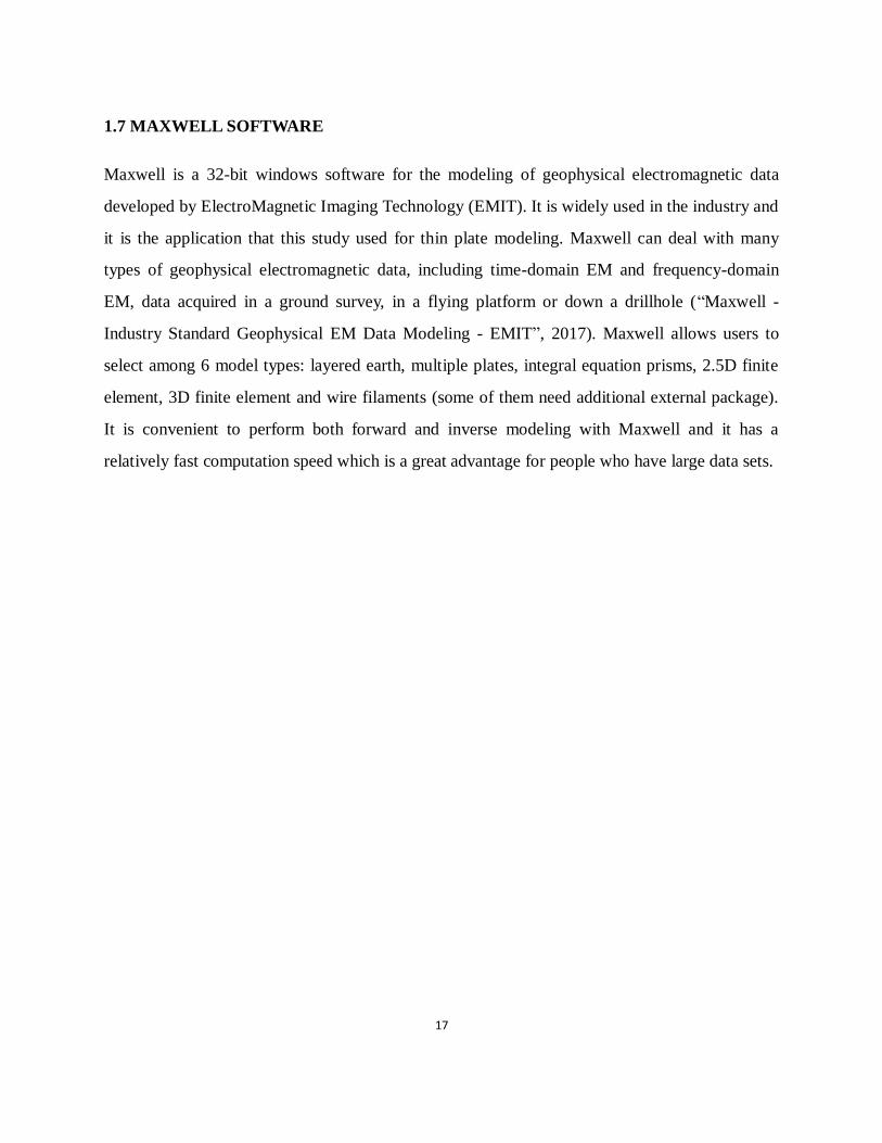
Then the plate obtained from Flight Line L30220 is used to check against tie line response (Tie
Line T30971) as shown in Figure 4.4.
It can be seen that this single plate model also has a good fit with the tie line field data.
Area 1
T30971
L30220

38
Figure 4.3 Plate modelling of L30220 (Channels 15-30 are shown)
39
Figure 4.4 Plate modelling of T30971 (Channels 15-30 are shown)

40
4.2.2 Area 2 thin plate modelling
Figure 4.5 shows the location of Area 2 where Flight Line L12080, L12090, L12100 and Tie
Line T19080 detected a coincident magnetic and electromagnetic anomaly.
A combined model using data from Flight Line L12080, L12090 and L12100 is created and two
plates are obtained as a result of Maxwell thin plate modelling (Figure 4.6).
Figure 4.5 Location of Area 2
As shown above in Figure 4.6, the red plate on the west has a depth of 21.6m, a strike length of
290m, a depth extent of 275m, a conductance of 69.5 Seimens and 65° dipping to the West; the
blue plate has a depth of 60m, a strike length of 277m, a depth extent of 210m, a conductance of
19.9 Seimens and is almost flat lying. Therefore the red conductor has a steep tilt angle and a
shallower depth to surface while the blue conductor is close to horizontal-lying at a larger depth
Area 2
T19080
L12080
L12100
L12090

41
and also less conductive.
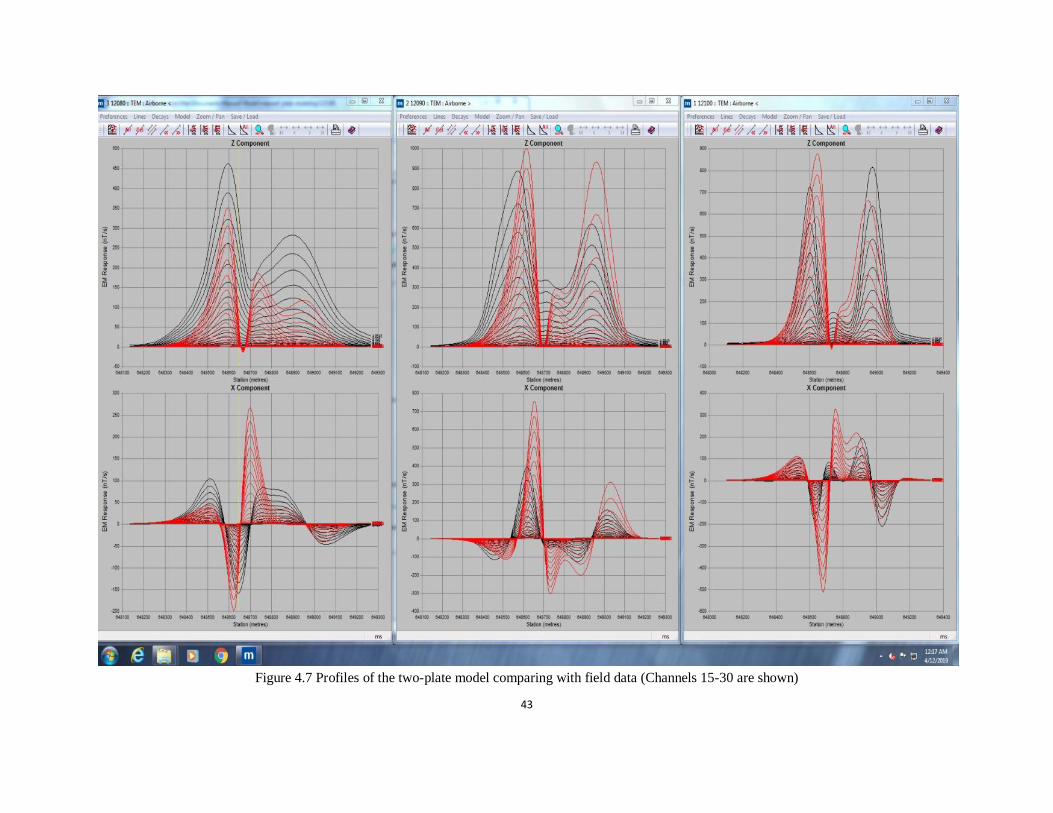
Figure 4.7 shows the Z component and X component electromagnetic response of this two-plate
model comparing with the field data along the Flight Line L12080, L12090 and L12100. It can
be told that the two-plate model has a reasonably good fit on all three flight lines.
Then the two plates obtained from the combined three flight line model are used to check against
tie line response (Tie Line T19080).
As shown in Figure 4.8, this two-plate model has a acceptably good fit with the tie line field data
as well.

42
Figure 4.6 Plate modelling of L12080, L12090, L12100
43
Figure 4.7 Profiles of the two-plate model comparing with field data (Channels 15-30 are shown)

44
Figure 4.8 Plate modelling of T19080 (Channels 15-30 are shown)

45
Chapter 5
Results
Two potential areas, Area 1 and Area 2, are demonstrated in chapter 4. Both magnetic anomalies
and electromagnetic anomalies are detected there and the electromagnetic anomalies are good for
the thin plate modelling. Depth estimate of the targets are conducted using magnetic data and
electromagnetic data separately in chapter 3 and chapter 4.
Figure 5.1 shows the depth estimate from the Radial Frequency Spectrum method applied to
magnetic data in Area 1. The first straight line segment in Figure 5.1 indicates a depth of 71.19m
from source to the magnetometer which reveals a depth of 36.19m from source to ground surface
(the magnetometer is 35m above ground). Figure 5.2 shows the depth estimate from the Radial
Frequency Spectrum method applied to magnetic data in Area 2 and it indicates the depth of the
target is 58m from source to the magnetometer and 23m from source to surface.
Figure 5.3 and Figure 5.4 display the results of the depth estimate of t ilt derivative method
applied to magnetic data in Area 1 and Area 2 separately. The perpendicular distance between 45°
and -45° contour lines indicates twice the depth and in this case Area 1 target has a depth of 58m
from source to ground surface and it is suggesting that the Area 2 target is at the surface.

46
Figure 5.1 Radial frequency spectrum method applied to magnetic data in Area 1
Figure 5.2 Radial frequency spectrum method applied to magnetic data in Area 2

47
Figure 5.3 Tilt derivative method applied to magnetic data in Area 1
Figure 5.4 Tilt derivative method applied to magnetic data in Area 2
A
No
rth
ing
Easting

48
Above results are compared with the Maxwell thin plate models obtained from electromagnetic
data in chapter 4 to make sure the magnetic anomalies and the electromagnetic anomalies are
reflecting the same source at the same depth (Table 5.1).
Depth from EM anomaly
Depth from MAG anomaly,
radial frequency spectrum
method
Depth from MAG
anomaly, tilt derivative
method
Area
1 53m top of conductor 36m 58m
Area
2
21m top of first conductor,
60m top of second
conductor
22m 0m
Table 5.1 Comparison of depth estimate from electromagnetic anomalies and magnetic anomalies
Both depth estimate methods used on the magnetic data have different assumptions and so some
differences in depths are expected. From the above table, depths from electromagnetic anomalies
are consistent with depths from magnetic anomalies in Area 1 and Area 2. Therefore it is
reasonable to say that Area 1 and Area 2 both have sources that are conductive and magnetic.
The two areas can be viewed as potential areas for VMS deposits and the Maxwell thin plate
models give us the potential targets’ orientation and size as well.

49
Chapter 6
Conclusions
In the HELITEM system, the transmitter and receiver coils are attached to a flying helicopter and
there is a coil coupling effect produced as a result of the motion of the receiving coil in the static
geomagnetic field. The industry assumes that this electromagnetic induction is a constant during
a pulse time and corrects it as a part of the leveling. However, in chapter 2 it is proved that the
coil coupling effect cannot be viewed as a constant during a pulse time especially in the case of
deposits with long time constants and high horizontal magnetic gradients.
Volcanogenic massive sulfide (VMS) deposits which are the potential targets in this study are
very likely to be conductive and magnetic at the same time compared to their hosting
environment. Figure 3.1 and figure 3.2 are the co-location maps of electromagnetic and magnetic
anomalies of Hollingdale Lake block and south Botham Bay block. Contour maps of residual
magnetic intensity (RMI) are used as base maps and the red circles indicate where
electromagnetic anomalies and magnetic anomalies exist at the same location, but not necessarily
at the same depth.
Chapter 3 applied radial frequency spectrum method and tilt derivative method separately to do
depth estimate using magnetic data. Chapter 4 used Maxwell thin plate modeling to do depth
estimate from electromagnetic data and plate modeling can also refine the conductor’s depth
extent, size, shape and conductivity. As a result, it is found that the depths from electromagnetic
anomalies are consistent with depths from magnetic anomalies in Area 1 (figure 4.2) and Area 2

50
(figure 4.5). Therefore the two areas both have targets that are conductive and magnetic at the
same time and can be viewed as potential areas for VMS deposits.
6.1 RECOMMENDATIONS
This study here investigated on an airborne magnetic and HELITEM survey on Flin Flon area
and provided a procedure to locate potential VMS deposits and refine the targets’depth,
orientation, depth extent, size, shape and conductivity. However, the thin plate modelling might
not perfectly describe the targets in the field. Further ground surveys are needed on the potential
areas.
To improve the performance and effectiveness of the HELITEM system, it is necessary to apply
a three component magnetometer instead of only measuring the total field of the magnetic data.
The coil coupling effect discussed in chapter 2 is not a huge problem. It won't cause a difference
at many places, but at places where the magnetic field is highly variable or where
electromagnetic time constants are relatively long, by correcting this effect in a better way could
provide better estimates of the time constant.
Only two anomalies were fully investigated. Both proved to be co-located in three dimensions as
magnetic and conductive targets. Therefore, a full investigation of other anomalies may discover
more co-located prospective targets.

51
REFERENCES
Adam, S. (2012). Detection of Perfect-conducting Targets with Airborne Electromagnetic
Systems. PhD thesis, University of Toronto.
Bob, L. (2014). Report on Thin Plate Modeling of VTEM data.
Comparison of different airborne TEM systems. Retrieved July 15, 2017 from
https://geomodel.info/tdem/help/en/airborne_tem.htm?id=1
Dawn, Z. (2013). Flin Flon Project 2013 Airborne Magnetic and HELITEM Survey Assessment
report.
Edward, R., Michael, C. (2018). Electromagnetics.
Flin Flon History. Retrieved July 16, 2017 from
https://www.cityofflinflon.ca/history-of-flin-flon
Fugro Airborne Surveys, Geophysical Survey Report to BFR Copper & Gold Inc. (2013)
Galley, A.G., Syme, E.C., & Bailes, A.H. (2007). Metallogeny of the Paleoproterozoic Flin Flon
Belt, Manitoba and Saskatchewan. In Goodfellow W.D. (ed.), Mineral Deposits of
Canada: A Synthesis of Major Deposit Types, District Metallogeny, the Evolution of
Geological Provinces, and Exploration Methods (pp. 509-531). Geological Association
of Canada.
Ghosh, M.K. (1972). Interpretation of Airborne EM (Electromagnetic) Measurements Based on
Thin Sheet Models. PhD thesis. University of Toronto.
Gibson, H. et al. (2013). Field Trip Guidebook -FT-C3: The Volcanological and Structural
Evolution of the Paleoproterozoic Flin Flon Mining District, Manitoba: The Anatomy of
a Giant VMS System Open File Report OF 2013-6.

52
Grant, F.S. & West, G.F. (1965). Interpretation Theory in Applied Geophysics. McGraw-Hil
Book Company.
Hunt, C.P., Moskowitz, B.M., and Banerjee, S.K. (1995). Magnetic properties of rocks and
minerals.InAhrens, T.J. (ed.),Rock physics and phase relations-A handbook of physical
constants(pp. 189–204). American Geophysical Union.
Jean, M.L. (2015). Airborne Electromagnetic Systems - State of the Art and Future Directions.
CSEG Recorder,40,No.6.
Jinming, L. (2005). Geoelectric Field and Electrical Exploration (p.2). Geological Publishing
House.
Keating, P.B. (1988). The Inversion of Time-domain Airborne Electromagnetic Data Using the
Plate Model. PhD thesis. McGill University.
Maxwell - Industry Standard Geophysical EM Data Modeling - EMIT. Retrieved from
http://www.electromag.com.au/maxwell.php
Merriam, J. (2018). General Rules for Depth Estimates. [Unpublished class notes].
Miller, H.G. and Singh, V. (1994). Potential field tilt - a new concept for the location of potential
field sources. Journal of Applied Geophysics, 32, 213-217.
Palacky, G.J. (1987). Resistivity characteristics of geologic targets. In M. Nabighian, editor,
Electromagnetic Methods in Geophysical Applications Volume 1, Theory, (pp. 53-129).
Society of Exploration Geophysicists.
Reynolds, J. (1997). An Introduction to Applied and Environmental Geophysics (pp. 15-89). John
Wiley.
Richard, S. (2010). Airborne electromagnetic methods: applications to minerals, water
andhydrocarbon exploration. CSEG Recorder, 3,7-10.

53
Robert S. Carmichael (1989). Practical handbook of physical properties of rocks and minerals.
CRC Press.
Salem, A., Williams, S., Fairhead, J. D., Ravat, D., and Smith, R. (2007). Tilt-depth method:A
simple depth estimation method using first-order magnetic derivatives, The Leading Edge,
26, 1502-1505.
Simard, R-L., MacLachlan, K., Gibson, H.L., DeWolfe, Y.M., Devine, C.A., Kremer, P.D.,
Lafrance B., Ames, D., Syme, E.C., Bailes, A.H., Bailey, K., Price, D., Pehrsson, S.,
Lewis, E.M., Lewis, D. and Galley, A.G. (2013). Geology of Flin Flon area, Manitoba
and Saskatchewan (parts of NTS 63K12, 13) (Geoscientific Report GR2012-2). Manitoba
Innovation, Energy and Mines, Manitoba Geological Survey.
Touloukian, Y. S., Judd, W. R., Roy, R. F. (1989). Physical Properties of Rocks and Minerals.
Purdue Research Foundation.
Yusheng, Z., Shuzhen, Y. & Keqin, C. (2011). Mineral Deposits (3rd Edition) (pp. 216-222).
Geological Publishing House.