1

Investigation of the genetic structure of some common bean (Phaseolus vulgaris L.) 1

commercial varieties and genotypes used as a genitor with SSR and SNP markers 2

3

4

Omer AVICAN1,2

and Behiye Banu BILGEN3,

* 5

6

7

1 Agricultural Biotechnology Department, Graduate School of Natural and Applied 8

Sciences, Tekirdağ Namık Kemal University, Tekirdağ, Turkey 9

2 May-Agro Seed Company, Bursa, Turkey 10

3 Agricultural Biotechnology Department, Faculty of Agriculture, Tekirdağ Namık 11

Kemal University, Tekirdağ, Turkey 12

13

14

*Correspondence: Dr. Behiye Banu Bilgen, Tekirdağ Namık Kemal University, Faculty 15

of Agriculture, Agricultural Biotechnology Department, Tekirdağ, Turkey. Tel: (+90) 16

282 250 22 91; Fax: (+90) 282 250 22 99; E-mail: bbilgen@nku.edu.tr 17

16-digit ORCID: 0000-0001-8323-2509 18

19

20

Acknowledgements 21

We gratefully acknowledge Hasan Ozgur SIGVA for scientific and technical support for 22

SNP analysis. 23

24

25

26

27

28

RESEARCH ARTICLE 29

30

31

32

2

Abstract 1

2

Common bean is a species belonging to the Phaseolus genus of the Leguminosae family. It has economic 3

importance due to being rich in protein, vitamin A and C, and minerals. Being one of the most cultivated 4

species of legumes, the determination of genetic diversity in bean genotypes or populations has an 5

important role in terms of our genetic resources. The objective of this study was to evaluate the genetic 6

structure of 94 genotypes which were cultivated in different parts of the world and our country with SSR 7

and SNP markers. 10 SSR loci and 73 SNP primers were used for the determination of genetic structure 8

in commercial cultivars and breeding lines. All of the SSR and SNP loci used in the study were found to 9

be polymorphic. A total of 89 alleles were identified for 10 SSR loci. Mean number of alleles per locus 10

(Na=8.9), effective allele number (Ne=3.731), Shannon information index (I=1.468), observed 11

heterozygosity (Ho=0.023), and expected heterozygosity (He=0.654) were calculated based on SSR 12

analysis. According to the results of Bayesian-based STRUCTURE analysis using SSR and SNP data, 94 13

bean genotypes were genetically divided into three main clusters. According to genetic similarity based 14

UPGMA dendrogram obtained from SSR and SNP analysis, 94 bean genotypes were divided into 2 main 15

clusters. The obtained results provide important information about the genetic structures of the studied 16

bean cultivars and breeding lines. With the obtained results, it will be possible to develop breeding 17

programs to develop new cultivars by using our gene resources. 18

19

Keywords: Bean breeding, genetic diversity, Phaseolus vulgaris, SSR, SNP 20

21

3

Introduction 1

2

Common bean (Phaseolus vulgaris L.) belongs to the Leguminosae family which consists of 727 genera 3

and approximately 19,000 species. Some economically important species such as beans, chickpeas, 4

lentils, soya, broad beans, and peas are members of this family. Five species belonging to the genus 5

Phaseolus were cultivated for human nutrition in the world (P. vulgaris, P. coccineus, P. acutifolius, P. 6

lunatus, and P. polyanthus (Gaitan-Solis et al. 2002; Lewis et al. 2005). Leguminosae is the second 7

largest flowering plant family with 1013 species belonging to 71 genera in Turkey. Around 400 of these 8

species are endemic to Anatolia with the rate of 40% endemism (Erik and Tarikahya 2004; Toksoy et al. 9

2015). 10

11

Phaseolus vulgaris is the most preferred type of bean species for economic and scientific 12

purposes. The P. vulgaris is native to America and it was believed that domestication occurs from 13

northern Andean and from Mesoamerican populations as two gene pools (Cortes 2013; Cortes and Blair 14

2017; Assefa et al. 2019). Common bean was brought to Europe at the beginning of the 16th century as an 15

ornamental plant. After the introduction of common bean lines, their agriculture increased over time and 16

started to be grown in almost every part of the world (Rodino and Drevon 2004). Common bean 17

cultivation in Turkey, especially for fresh pod and dry seed, dates back to the 17th century (Bozoglu and 18

Sozen 2007). 19

20

Common bean is an important part of the human diet due to its higher protein content (>22% of 21

their dry weight) compared to some cereals such as rice and wheat (Alzate-Marin et al. 2003; 22

Chandrakanth and Hall 2008). The fresh pods and seeds of common bean have approximately 90% water, 23

and they are rich in A and C vitamins. Due to the high nutritional value, being suitable for consumption in 24

different ways (fresh, dry, canned, pickled, etc.), being rich in minerals such as phosphorus and iron 25

besides its protein source, common bean is one of the vegetables with the highest consumption in our 26

country (Akcin 1973). The bean, which has an important position in agricultural production, stands out 27

because it contains the protein, vitamins, complex carbohydrates, and minerals (Ca, Mg, K, Cu, Fe, Mg, 28

and Zn) necessary for a healthy life (Miklas et al. 2006; Marotti et al. 2007; Blair 2013). In addition to 29

being consumed as a nutrient, beans are an important type of plant due to enriching the structure of the 30

soil, increasing the amount of organic matter in the soil, accumulating nitrogen, and using plant residues 31

as a component of commercial feed mixtures (Smith and Huyser 1987). 32

33

Fresh common bean production in Turkey is 547,349 tons and dry bean production is 279,518 34

tons annually (TUIK, 2020). Phaseolus vulgaris is the most cultivated legume plant in the world with 35

19,042,406 tons of fresh pods and 20,698,984 tons of dry seed production (Blair et al. 2006; Galvan et al. 36

2006; Miklas et al. 2006; Benchimol et al. 2007). The top three producers of fresh beans in the world are 37

China, Indonesia, and Turkey according to average production from 1994 to 2018. In addition, India, 38

Brazil, and Myanmar take the first three places in the average production of dry beans for the 1994-2018 39

4

range (FAO 2019). The large genetic diversity of beans is one of the reasons for such wide cultivation in 1

the world and Turkey and also the increased usage of common bean in breeding studies over the years. 2

3

Turkey is significantly rich in plant genetic resources due to its location at the crossroads of the 4

Mediterranean and the Near East gene centers. Moreover, Turkey has extensive biodiversity in terms of 5

habitat types, geomorphological structure, climate, and topographic features (Özhatay and Byfield 2005; 6

Özhatay et al. 2011). To protect the plant gene resources of our country, it is necessary to determine the 7

genetic diversity, genetic and morphological characterizations of our plant resources and also evaluate the 8

potentials of the species for various studies such as breeding. Especially with the advances in molecular 9

biology and genetics in the last 50 years, the emergence and development of modern biotechnology have 10

gained importance. The recent developments in DNA marker technology has reached high levels and has 11

provided valuable tools in various genetic analyses, from phylogenetic analysis to the cloning of genes. It 12

is possible to easily determine the genetic structure, create molecular maps, and label the characters of 13

interest by PCR-based markers. Researchers have utilized various molecular markers to conduct 14

molecular genetic studies in common bean populations/genotypes (Metais et al. 2001, 2002; Duran et al. 15

2005; Sicard et al. 2005; Angioi et al. 2010; Buah et al. 2017; Carucci et al. 2017). 16

17

In Turkey, the number of studies in which bean gene resources are defined by morphological or 18

molecular methods has started to increase in recent years. In this study, the aims were: 1) to identify the 19

genetic structure of studied common bean cultivars and breeding lines by SSR and SNP markers, 2) to 20

determine lines that can be used for the establishment of breeding programs by revealing genetic 21

relationships between studied common bean cultivars and breeding lines. 22

23

Materials and methods 24

25

Plant materials 26

27

In this study, a total of 94 bean genotypes (Phaseolus vulgaris, Phaseolus acutifolius, and Phaseolus 28

coccineus) were used. These included 79 commercial bean varieties that were cultivated in different 29

regions of the world and Turkey and 15 breeding lines used in our breeding programs. The bean 30

genotypes included in the study were P. vulgaris nanus: Determinate-Bush and P. vulgaris comminus: 31

Indeterminate-Climber bean forms (Table 1). Each bean genotype was grown in the greenhouse under 32

controlled conditions. Fresh leaf samples (300 mg) from 94 genotypes were collected in a 96-well Qiagen 33

tissue collection plate and they were stored at - 80ºC until DNA extraction. 34

35

DNA extraction 36

37

5

DNA extraction was performed with Qiagen DNA Extraction Instrument (QIAcube-HT). Each tissue 1

sample was ground using Tissue Lyser II for 2 min. The quantification and qualification of isolated DNAs 2

were performed with Thermo Scientific™ NanoDrop™ One Microvolume UV-Vis Spectrophotometer. 3

The DNA samples were preserved at - 20ºC till PCR analysis. 4

5

SSR analysis 6

7

Ten SSRs (BM141, BM143, BM152, BM160, BM172, GATS91, PV-at002, PV-ctt001, PV-ag001, and 8

PV-at007) were used for the genetic characterization of P. vulgaris genotypes (Yu et al. 2000; Gaitan-9

Solis et al. 2002). The fluorescently-labeled M13-tailed primer method was used for PCR amplification 10

(Schuelke 2000). The characteristics of the SSR primers were indicated in Table 2. 11

12

The PCR amplifications were performed as described in Yu et al. (2000) and Gaitan-Solis et al. 13

(2002) with the Applied Biosystems® Veriti™ Thermal Cycler. PCR products were controlled by 2% 14

agarose gel electrophoresis (1X TBE buffer, 110 V, 120 min). Gel Imaging System Vilber Lourmat 15

Quantum ST5 was used to visualize the agarose gels. The size of SSR fragments was determined by 3500 16

Genetic Analyzer (Applied Biosystems, Life Technologies, UK) capillary electrophoresis and 17

GeneMapper Software 5.0 (Applied Biosystems). 18

19

SNP Analysis 20

21

128 SNP loci represented 11 P. vulgaris chromosomes were selected from Blair et al. (2013) for 22

genotyping of 94 bean samples. For the SNP analysis Roche LightCycler® DNA Master HybProbe 23

Master Mix and ROCHE -LightCycler® 480 Instrument II Real Time PCR were used. 24

25

Data analysis 26

27

For each SSR locus, observed allele size range (bp) and observed allele number were determined. In 28

statistical analysis of SSR data, allele frequencies, allele numbers (Na), effective allele numbers (Ne), 29

Shannon’s information index (I), heterozygosity levels (Ho and He), and polymorphic information 30

contents (PIC) were estimated by the software GenAlEx Version 6.3 (Peakall and Smouse 2006). 31

32

Population structure based on SSR and SNP data was evaluated using STRUCTURE 2.3.4 33

(Pritchard et al. 2000) as described in Blair et al. (2009). Analyses had a burn-in length of 50,000 34

iterations and a run length of 100,000 iterations after burning. Ten replicates were carried out for each K 35

value (K=1 to K=10) (Evanno et al. 2005). STRUCTURE HARVESTER was used in order to determine 36

the best K value (Earl and vonHoldt 2012). NTSYS-pc Version 2.2 was used to analyse SSR data and 37

construct a dendrogram (Rohlf 2002). 38

6

1

In the SNP analysis, after the Real Time PCR process was completed, the genotypes in the SNP 2

region were determined by Melting Point analysis. The binomial data matrix was created by scoring the 3

raw data obtained in the SNP analysis according to present (1) or absent (0). NTSYS-pc Version 2.2 4

computer program was used to evaluate the distance matrix and dendrograms (Rohlf 2002). Phylogenetic 5

trees were created using UPGMA and SAHN grouping programs in grouping similar data to create 6

similarity dendrograms of the studied genotypes. 7

8

Results 9

10

The polymorphism level of studied 10 SSR loci was estimated as 100%. Totally 89 alleles (mean value = 11

8.9 alleles/locus) were determined. Evaluating all studied commercial varieties and breeding lines, 12

BM141, GATS91, and PV-at007 loci have the highest number of alleles (13 alleles), and BM160 has the 13

lowest number of alleles (3 alleles). 11 alleles were observed in BM143 and BM152 loci. The remaining 14

SSR loci have 7 or 6 alleles (Table 3). Table 3 indicates genetic diversity parameters estimated in the 15

studied P. vulgaris genotypes with 10 SSR loci. PIC values were calculated for SSR loci ranged from 16

0.854 to 0.289. The mean PIC value was estimated relatively high (0.621). Based on SSR analysis, the 17

overall mean number of effective alleles per locus (Ne) was 3.731 ± 0.628 (varied from 1.440 to 7.539). 18

The overall average value of Shannon’s information index (I) was calculated as 1.468. The highest value 19

of I was observed in the GATS91 locus (2.211) and the lowest in the BM160 locus (0.579). Estimated 20

values of mean expected heterozygosity (He) and observed heterozygosity (Ho) were 0.654 and 0.023, 21

respectively (Table 3). 22

23

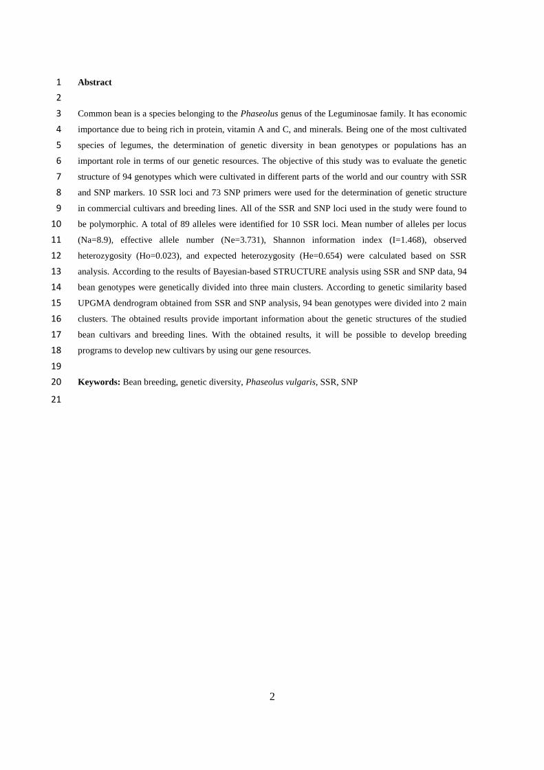
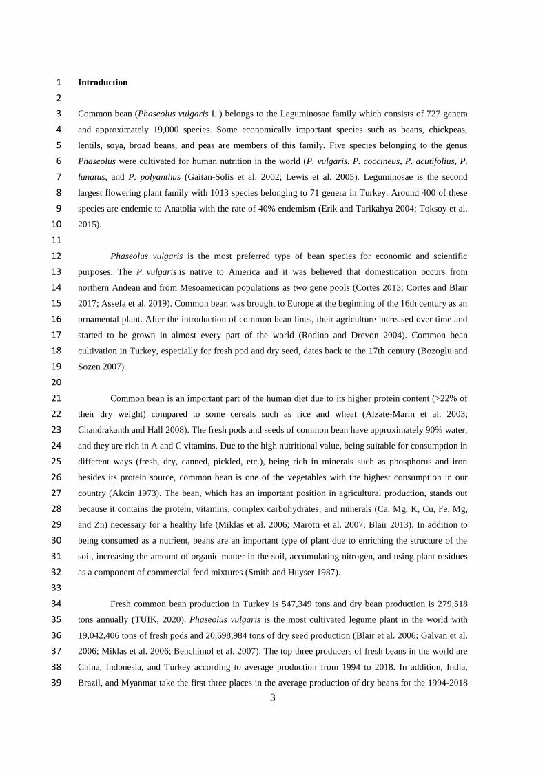
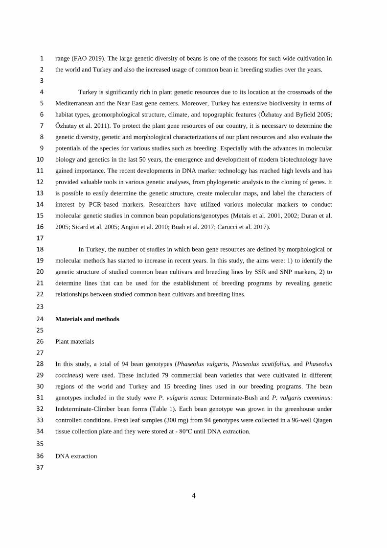
The ideal K value was calculated by STRUCTURE HARVESTER (Earl and vonHoldt 2012) 24

program in the SSR based STRUCTURE analysis for 94 different genotypes (Pritchard et al. 2000). The 25

optimal number of subpopulations was found for K = 3 (Fig. 1). Bayesian-based STRUCTURE analysis 26

showed that 94 bean genotypes were distributed between 3 main groups (Fig. 2). NTSYS-pc Version 2.2 27

was used to evaluate the distance matrix and dendrogram (Fig. 3). Genetic diversity was found in the 28

range of 0.17 - 1.0 for all studied bean genotypes. Some of the genotypes such as OT1/SK15, SK11/SB2, 29

OT28/SK7/SB7, OB3A/ST3 had genetic diversity value of 1.0. Two main clusters were observed for 94 30

bean genotypes in the diversity matrix based dendrogram. Cluster-1 had 7 genotypes and Cluster-2 with 3 31

subgroups had 87 genotypes. 32

33

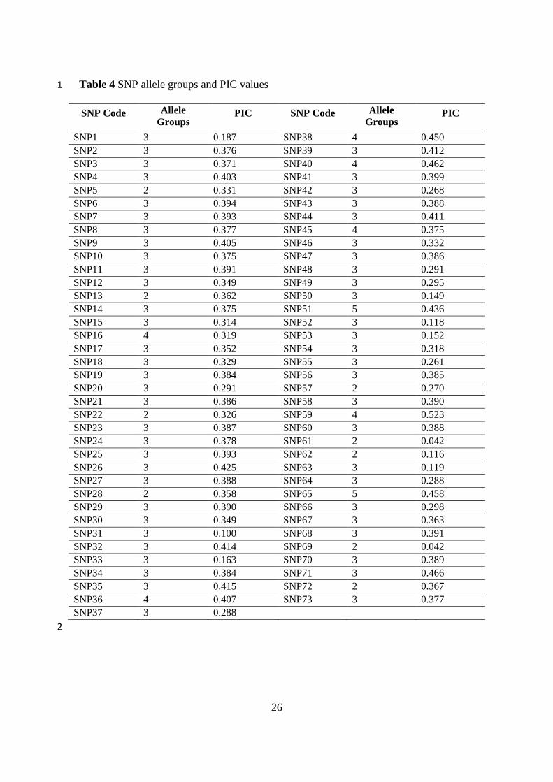
According to SNP analysis, 73 out of 128 studied SNP primers were polymorphic for the studied 34

P. vulgaris genotypes. Evaluating polymorphic SNP primers’ melting peak profiles, with each peak as an 35

allele, revealed highest allele group for SNP51 and SNP65 (5 alleles) primers. SNP13, SNP22, SNP28, 36

SNP61, SNP62, SNP69 and SNP72 primers had the lowest allele groups (2 alleles). The number of allele 37

groups and PIC values for SNP primers were given in Table 4. Calculated PIC values were varied 38

7

between 0.042 and 0.523. The mean PIC value was 0.337. SNP59 has the highest PIC value (0.523), 1

whereas SNP61 and SNP69 had the lowest PIC value (0.042). 2

3

The binomial data matrix was created by scoring the raw data obtained in the SNP analysis 4

according to the presence (1) or absence (0). The ideal K value was calculated by STRUCTURE 5

HARVESTER (Earl and vonHoldt 2012) program in the SSR based STRUCTURE analysis for 94 6

different genotypes (Pritchard et al. 2000). The optimal number of subpopulations was found for K = 3 7

(Fig. 4). Bayesian-based STRUCTURE analysis showed that 94 bean genotypes were distributed between 8

3 main groups (Fig. 5). NTSYS-pc Version 2.2 was used to evaluate the distance matrix and 9

dendrograms. The dendrogram created as a result of the SNP analysis is given in Figure 6. When the 10

dendrogram was examined, it was observed that the genetic diversity varied between 0.46 and 1.00. 94 11

bean genotypes used in the study are divided into 2 main clusters in the dendrogram. At the same time, 12

the two main clusters were divided into subgroups, differentiating bean varieties to a large extent and 13

gave successful results in obtaining the expected subgroups. The degree of kinship of bean genotypes was 14

determined with the help of Euclidean similarity index coefficients, and 3D graphics were created for 15

SNP (Fig. 7). Clusters formed by the studied bean genotypes were observed in accordance with the results 16

in UPGMA dendrograms. 17

18

Discussion 19

20

DNA fingerprinting studies using molecular markers (especially SSR and SNP markers) have a high 21

impact on revealing the differences between genotypes (Assefa et al. 2019). In this study, important 22

information about the genetic structure of 94 genotypes from commercial bean varieties and breeding 23

genotypes cultivated in the world and different regions of Turkey has been obtained via molecular 24

markers. 89 polymorphic bands were obtained by using 10 SSR primers. The mean number of 25

polymorphic bands per primer is 8.9. Blair et al. (2006) were performed SSR analysis (129 SSRs) in order 26

to determine the genetic structure of 43 P. vulgaris genotypes and 1 P. acutifolius obtained from different 27

regions of America, and the polymorphism rate obtained with genomic microsatellites was determined as 28

(0.446). In the study of Kwak et al. (2009), the average number of alleles was determined as 16 with 26 29

SSRs in bean genotypes collected from different geographical regions. Burle et al. (2010) were analysed 30

67 SSRs in 279 bean genotypes collected from Brazil and the average number of alleles was calculated as 31

6. Since Brazil is one of the gene centers of the bean, high genetic diversity has been reported among the 32

genotypes there. In Cabral et al. (2011), 16 SSR markers were used to determine genetic diversity in 57 33

bean genotypes collected from the Brazilian region, 13 SSRs were found to be polymorphic, and the 34

number of alleles obtained from these markers was calculated as 29 and the average number of alleles per 35

locus was calculated as 2.2. Khaidizar et al. (2012) reported 72 alleles at 30 SSR loci in bean genotypes 36

sampled from North Anatolia. Bilir et al. (2019), a total of 192 alleles were identified in 13 SSR markers, 37

and the average number of alleles per locus was reported as 14.8. In the study of Ekbic and Hasancaoglu 38

8

(2019), it was stated that 63 alleles (polymorphism rate 73%) belonging to 18 SSR loci in bean genotypes 1

and the average number of alleles per locus was 2.55. The average number of polymorphic bands 2

obtained by the researchers is close to the values we obtained from this study. 3

4

Shannon information index (I), which is one of the genetic diversity parameters, was calculated 5

from 0.579 to 2.211. Hence, this high I value (mean 1.468) indicates high variation within genotypes. The 6

mean observed heterozygosity (Ho) was calculated as 0.023 and the mean expected heterozygosity (He) 7

was calculated as 0.654. Since the genotypes used in this study belongs to commercial varieties and 8

breeding materials, most of the samples have homozygous genotypes and therefore Ho was low. In Bilir 9

et al. (2019), the observed heterozygosity was calculated as 0.452 and the expected heterozygosity was 10

0.724. Valentini et al. (2018) reported that genetic diversity (h) on 18 SSR loci in 109 bean genotypes 11

sampled from Brazil was 0.44. In Valentini et al. (2018), 4 groups were observed in which two Andean 12

and two Mesoamerican genotypes clustered within themselves at K=4. Pereira et al. (2019) reported He 13

as 0.55 and Ho as 0.05 in 17 bean varieties. Pereira et al. (2019) using the toucher method and evaluating 14

27 SSR loci, 17 bean genotypes formed 4 different groups in their clustering analysis. In the study of 15

Carucci et al. (2017), the genetic structure of Italian local bean cultivars was analysed with 12 SSR loci, 16

the Ho value was calculated as 0.24. 17

18

According to the results of the Bayesian-based STRUCTURE analysis based on the SSR data 19

conducted within the scope of the study, 94 bean genotypes were genetically divided into 3 main groups. 20

However, phylogenetic trees were created using UPGMA and SAHN grouping gave 2 main groups. 21

When the results of STRUCTURE analysis and UPGMA dendrogram were compared, it has been 22

observed that obtained SSR data could not able to differentiate bean genotypes exactly. Such a result may 23

be due to the type and number of markers selected and used in this study. Therefore, it was planned to 24

select and use a different marker type and SNP analysis was performed. Burle et al. (2010) reported that 25

279 bean genotypes found in Brazil were divided into two groups (K=2), Andean and Mesoamerican, as a 26

result of STRUCTURE analysis. Blair et al. (2012) reported that 108 bean genotypes were divided into 5 27

groups as Andean, Colombian, Ecuadorian, Northern Peruvian, Guatemalan, and Mesoamerican. 28

29

For SNP analysis, 73 of 128 SNP primers were selected from different regions of 11 30

chromosomes of P. vulgaris, and they were determined as polymorphic. The mean PIC value was 31

calculated as 0.337. In Cortes et al. (2011), the SNP diversity was performed in beans, the mean PIC 32

value of 94 SNP primers in 70 bean genotypes (28 Andean and 42 Mesoamerican) was reported as 0.437. 33

In the study, 2 main clusters with Andean and Mesoamerican gene pools were observed in 70 bean 34

genotypes cultured and it was reported that SNP analysis differentiated these groups as expected. Blair et 35

al. (2013), in a study conducted on P. vulgaris to screen for parental polymorphism and to determine 36

genetic diversity, 736 SNPs were primarly scored in 236 different bean genotypes and the mean PIC 37

value was calculated as 0.328. The mean PIC value of the SNP primers we used in our study was 38

determined between the average PIC values obtained by Cortes et al. (2011) and Blair et al. (2013). SNP 39

9

markers are highly sensitive markers based on single nucleotide polymorphism, and also the SNP primers 1

have a very high power to discriminate between genotypes/populations. In the study conducted by Nemli 2

(2013), 105 SNP markers were used to determine genetic diversity in 66 bean genotypes. The PIC values 3

obtained in the study were calculated between 0.97 and 0.04 (mean PIC value=0.65). 4

5

According to the results of the Bayesian-based STRUCTURE analysis based on the SNP data, 94 6

bean genotypes were genetically divided into 3 main groups. UPGMA dendrogram gave 2 main groups. 7

Based on the dendrogram created as a result of SNP analyses, it was observed that the genetic diversity 8

ranged between 0.46 and 1.00. When the dendrogram and STRUCTURE results were examined in detail, 9

it has been observed that obtained SNP data could differentiate bean genotypes successfully as expected. 10

In addition, the genotypes of P. acutifolius and P. coccineus species used as standard (control) varieties 11

appeared in separate groups. Thus, SNP is an efficient and effective approach for genotyping the bean 12

genotypes and analysing genetic relatedness for large-scale screening. In Cortes et al. (2011), KASPar 13

technology was used to develop SNP markers in 70 bean genotypes belonging to the Andean and 14

Mesoamerican gene pools. In that study, 84 genomic and 10 EST-SNP markers were developed and it 15

was reported that the Mesoamerican and Andean gene pools were successfully separated using these 16

primers. Compared to the Mesoamerican gene pool, more diversity was observed in individuals belonging 17

to the Andean gene pool. In addition, it has been reported that SSR and SNP markers are ideal markers 18

when used together in bean diversity studies. 19

20

Various DNA marker systems are used in genetic diversity studies, and the comparison of the 21

use of these systems is extremely important for molecular plant breeding studies and analysis. 22

Interlaboratory transfer of the DNA marker systems is necessary for standardization and comparison of 23

the data obtained in order to obtain reproducible results. Thus, the financial costs of the work done are 24

reduced and time can be saved. Garcia et al. (2004) used different marker systems (SSR, RFLP, AFLP, 25

and RAPD) to determine genetic diversity in tropical maize species. Geleta et al. (2006) reported that 26

both SSR and AFLP techniques were effective in their genetic diversity study among Sorghum 27

genotypes. Cortes et al. (2011) reported that SSR and SNP markers are ideal markers when used together 28

in diversity studies in beans. In the study conducted by Ulukapı and Onus (2012), genetic analyses were 29

made using SCAR and SSR markers in beans, and a UPGMA dendrogram was created based on SCAR 30

and SSR data of 39 genotypes. 31

32

Although the classical breeding studies in many agricultural plant species have reached the 33

desired rate, the use of molecular markers in the development of new genotypes and varieties has made 34

significant contributions to breeding programs. Classical and molecular breeding programs are created by 35

adding DNA markers that provide valuable data to existing breeding programs that are developing very 36

rapidly. It is important to reveal the genetic relationship between bean species, breeding lines under 37

development in bean breeding programs, and existing commercial bean varieties in detail, as well as in 38

family selections, genetic analyses for various purposes, and in the planning of breeding programs. 39

10

Genetic diversity analyses of owned gene resources also allow the use of data at molecular, geographic, 1

functional, and morphological levels (Lu et al. 2009). Genetic distance and proximity studies provide the 2

emergence of differences between the studied genotypes and contribute to increasing the genetic diversity 3

in the gene pool in breeding programs. The more genetic distance the genotypes have from each other, the 4

greater the variation seen. These openings seen in breeding genotypes shape the selection and the more 5

variation is obtained, higher the chance of success of the breeding program, which makes it easier for the 6

breeder to reach the goal. Performing genetic analyses in genetic diversity studies, determining distance 7

and proximity conditions, contributes to the creation of new populations and to obtain high yielding 8

combinations with heterosis. Plant breeders use the evaluation of genetic diversity using various methods 9

as an alternative selection method, the genetic diversity data obtained helps to organize the studied 10

genotypes into groups. Thus, the creation of the most promising hybrid combinations among genotypes 11

with known morphological, agronomic, and genetic features allows the creation of combinations that can 12

be cost and time effective (Souza et al. 2008). In this study, it was aimed to determine the genetic 13

closeness-distances by obtaining the bean species, breeding lines and commercial varieties, and 14

phylogenetic tree from the data obtained by using molecular methods and to use these data in the breeding 15

program. The importance of the study is clearly revealed, as it reveals the possibility of increasing the 16

chance of success both in the selections to create new strong populations and in the selections in the 17

formation of productive hybrids, by revealing the kinship relations between the lines via molecular 18

markers. 19

20

Declarations 21

Funding: This study was funded by Tekirdağ Namık Kemal University, Scientific Research Projects Unit 22

(Project No: NKUBAP.03.YL.18.171). 23

24

Compliance with ethical standards 25

26

Conflict of interest: The authors declare that they have no conflict of interest. 27

28

Research involving human participants or animals: This article does not contain any studies with 29 human participants or animals performed by any of the authors. 30 31

References 32

Akcin A (1973) Erzurum şartlarında yetiştirilen kuru fasulye çeşitlerinde gübreleme. ekim zamanı ve sıra 33

aralığının tane verimine etkisi ile bu çeşitlerin bazı fenolojik. morfolojik ve teknolojik karakterleri 34

üzerine bir araştırma. Atatürk Üniversitesi Ziraat Fakültesi Dergisi 4(2):65-76. (In Turkish) 35

Alzate-Marin A, Costa M, Sartorato A, Peloso J, Borro E, Moreira M (2003) Genetic variability and 36

pedigree analysis of Brazilian common bean elite genotypes. Scientia Agricola 60(2):283-290. 37

11

Angioi S A, Rau D, Attene G, Nanni L, Bellucci E, Logozzo G, Negri V, Spagnoletti Z, PL Papa R 1

(2010) Beans in Europe: origin and structure of the European landraces of Phaseolus vulgaris L. 2

Theor Appl Genet 121:829-843. 3

Assefa T, Mahama AA, Brown AV, Cannon EKS, Rubyogo JC, Rao IM, Blair MW, Cannon SB (2019) 4

A review of breeding objectives, genomic resources and marker-assisted methods in common 5

bean (Phaseolus vulgaris L.). Mol Breeding 39:20. 6

Benchimol LL, Campos T, Carbonell SAM, Colombo CA, Chioratto AF, Formighieri EF, Souza AP 7

(2007) Structure of genetic diversity among common bean (Phaseolus vulgaris L.) varieties of 8

Mesoamerican and Andean origins using new developed microsatellite markers. Genet Resour 9

Crop Evol 54:1747-1762. 10

Bilir O, Yuksel Ozmen C, Ozcan S, Kibar U (2019) Genetic analysis of Turkey common bean (Phaseolus 11

vulgaris L.) genotypes by simple sequence repeats markers. Russian Journal of Genetics, 55:61-12

70. 13

Blair MW, Giraldo MC, Buendia HF, Tovar E, Duque MC, Beebe SE (2006) Microsatellite marker 14

diversity in common bean (Phaseolus vulgaris L.). Theor Appl Genet 113:100-109. 15

Blair MW, Diaz LM, Buendia HF, Duque MC (2009) Genetic diversity. seed size associations and 16

population structure of a core collection of common beans (Phaseolus vulgaris L.). Theor Appl 17

Genet 119:955-972. 18

Blair MW, Soler A, Cortes AJ (2012) Diversification and population STRUCTURE in common beans 19

(Phaseolus vulgaris L.). PLoS ONE, 7(11): e49488. 20

Blair MW (2013) Mineral biofortification strategies for food staples: The example of common bean. J 21

Agric Food Chem 61:8287-8294. 22

Blair MW, Cortes AJ, Penmetsa RV, Farmer A, Carrasquilla-Garcia N, Cook DR (2013) A high-23

throughput SNP marker system for parental polymorphism screening and diversity analysis in 24

common bean (Phaseolus vulgaris L.). Theor Appl Genet 126(2):535-48. 25

Bozoglu H, Sozen O (2007) Some agronomic properties of the local population of common bean 26

(Phaseolus vulgaris L.) of Artvin province. Turk J Agric For 31:327-334. 27

Buah S, Buruchara R, Okori P (2017) Molecular characterisation of common bean (Phaseolus vulgaris 28

L.) accessions from southwestern Uganda reveal high levels of genetic diversity. Genet Resour 29

Crop Evol 64:1985-1998. 30

Burle ML, Fonseca JR, Kami JA, Gepts P (2010) Microsatellite diversity and genetic STRUCTURE 31

among common bean (Phaseolus vulgaris L.) landraces in Brazil, a secondary center of diversity. 32

Theor Appl Genet 121:801-813. 33

Cabral PDS, Soares TCB, Lima ABP, De Miranda FD, Souza FB, Gonçalves LSA (2011) Genetic 34

diversity in local and commercial dry bean (Phaseolus vulgaris) accessions based on 35

microsatellite markers. Genetics and Molecular Research 10(1):140-149. 36

Carucci F, Garramone R, Aversano R, Carputo D (2017) SSR markers distinguish traditional Italian bean 37

(Phaseolus vulgaris L.) landraces from Lamon. Czech J Genet Plant Breed 53(4):168-171. 38

Chandrakanth E, Hall TC (2008) Phaseolin: structure and evolution. The Open Evolution Journal 2:66-74. 39

12

Cortes AJ, Blair MW (2017) Lessons from common bean on how wild relatives and landraces can make 1

tropical crops more resistant to climate change. In: Grillo O (ed) Rediscovery of landraces as a 2

resource for the future. InTech ISBN 978-953-51-5806-6 3

Cortes AJ, Chavarro MC, Blair MW (2011) SNP marker diversity in common bean (Phaseolus vulgaris 4

L.). Theor Appl Genet 123:827-845. 5

Cortes AJ (2013) On the origin of the common bean (Phaseolus vulgaris L.) American Journal of Plant 6

Sciences 4:1998-2000. 7

Duran LA, Blair MW, Giraldo MC, Macchiavelli R, Prophete E. Nin JC, Beaver JC (2005) 8

Morphological and molecular characterization of common bean landraces and cultivars from the 9

Caribbean. Crop Science 45:1320-1328. 10

Earl DA, vonHoldt BM (2012) STRUCTURE HARVESTER: A website and program for visualizing 11

STRUCTURE output and implementing the Evanno method. Conserv Genet Resour 4:359-361. 12

Ekbic E, Hasancaoglu EM (2019) Morphological and molecular characterization of local common bean 13

(Phaseolus vulgaris L.) genotypes. Applied Ecology and Environmental Research 17(1):841-853. 14

Erik S, Tarikahya B (2004) Türkiye florası üzerine. Kebikeç 17:139-163 (in Turkish). 15

Evanno G, Regnaut S, Goudet J (2005) Detecting the number of clusters of individuals using the software 16

STRUCTURE: a simulation study. Mol Ecol 14:2611-2620. 17

FAO 2019 Food and Agriculture Organization of the United Nations. FAOSTAT statistical database. 18

[Rome]:FAO. 19

Gaitan-Solis E, Duque MC, Edwards KJ,. Tohme J (2002) Microsatellite repeats in common bean 20

(Phaseolus vulgaris): isolation, characterization, and cross-species amplification in Phaseolus 21

spp. Crop Science 42:2128-2136. 22

Galvan MZ, Menendez-Sevillano MC, De Ron AM, Santalla M, Balatti PA (2006) Genetic diversity 23

among wild common beans from northwestern Argentina based on morpho-agronomic and RAPD 24

data. Genet Resour Crop Evol 53:891-900. 25

Garcia AAF, Benchimol LL, Barbosa AMM, Geraldi IO, Junior CLS, Souza AP (2004) Comparison of 26

RAPD, RFLP, AFLP and SSR markers for diversity studies in tropical maize inbred lines. Genet 27

Mol Biol 27:579-588. 28

Geleta N, Labuschagne MT, Viljoen CD (2006) Genetic diversity analysis in sorghum germplasm as 29

estimated by AFLP, SSR and morpho-agronomical markers. Biodivers Conserv 15:3251. 30

Khaidizar MI, Haliloglu K, Elkoca E, Aydın M, Kantar F (2012) Genetic diversity of common bean 31

(Phaseolus vulgaris L.) landraces grown in Northeast Anatolia of Turkey assessed with simple 32

sequence repeat markers. Turkish Journal of Field Crops 17(2):145-150. 33

Kwak M, Gepts P (2009) Structure of genetic diversity in the two major gene pools of common bean 34

(Phaseolus vulgaris L., Fabaceae). Theor Appl Genet 118(5):979-992. 35

Lewis G, Schrire B, Mackinder B, Lock M (2005) Legumes of the World. Kew. UK: Royal Botanical 36

Gardens. 37

Lu Y, Yan J, Guimaraes CT, Taba S, Hao Z, Gao S, Chen S, Li J, Zhang S, Vivek BS, Magorokosho C, 38

Mugo S, Makumbi D, Parentoni SN, Shah T, Rong T, Crouch JH, Xu Y (2009) Molecular 39

13

characterization of global maize breeding germplasm based on genome-wide single nucleotide 1

polymorphisms. Theor Appl Genet 120:93-115. 2

Marotti I, Bonetti A, Minelli M, Catizone P, Dinelli G (2007) Characterization of some Italian common 3

bean (Phaseolus vulgaris L.) landraces by RAPD, Semi-Random and ISSR molecular markers. 4

Genet Resour Crop Evol 54:175-188. 5

Metais I, Aubry C, Hamon B, Jalouzot R, Peltier D (2001) Assessing common bean genetic diversity 6

using RFLP, DAMD-PCR, ISSR, RAPD and AFLP markers. Acta Hort (ISHS) 546:459-461. 7

Metais I, Hamon B, Jalouzot R, Peltier D (2002) Structure and level of genetic diversity in various bean 8

types evidenced with microsatellite markers isolated from a genomic enriched library. Theor Appl 9

Genet 104(8):1346-1352. 10

Miklas PN, Kelly JD, Beebe SE, Blair MW (2006) Common bean breeding for resistance against biotic 11

and abiotic stresses: from classical to MAS breeding. Euphytica 147:105-131. 12

Nei M (1987) Molecular Evalutionary Genetics. Columbia University Press, NY. 512 p. 13

Nemli S (2013) Fasulye (Phaseolus vulgaris L.)’de Ekonomik Öneme Sahip Bazı Agronomik 14

Karakterleri Kontrol Eden DNA Markırlarının İlişki Haritalaması ile Saptanması. Doktora Tezi, 15

Ege Üniversitesi Fen Bilimleri Enstitüsü, İzmir. 16

Özhatay N, Byfield A (2005) Türkiye’nin önemli bitki alanı. Doğal Hayatı Koruma Vakfı 476s. İstanbul. 17

Özhatay FN, Kültür Ş, Gürdal MB (2011) Check-list of additional taxa to the supplement flora of Turkey 18

V. Turkish Journal of Botany 35:589-624. 19

Peakall R, Smouse PE (2006) GENALEX 6: Genetic Analysis in Excel. Population Genetic Software for 20

Teaching and Research. Molecular Ecology Notes 6:288-295. 21

Pereira HS, Mota APS, Rodrigues LA, de Souza TLPO, Melo LC (2019) Genetic diversity among 22

common bean cultivars based on agronomic traits and molecular markers and application to 23

recommendation of parent lines. Euphytica 215:38. 24

Pritchard JK, Stephens M, Donnelly P (2000) Inference of population structure using multilocus genotype 25

data. Genetics 155:945-959. 26

Rodino AP, Drevon JJ (2004) Migration of a grain legume Phaseolus vulgaris in Europe. In: Werner 27

D. (eds) Biological Resources and Migration. Springer, Berlin, Heidelberg 28

Rohlf FJ (2002) NTSYS-pc: Numerical Taxonomy System Version 2.1. Setauket: Exeter. 29

Schuelke M (2000) An Economic Method for the Fluorescent Labeling of PCR Fragments. Nature 30

Biotechnology 18:233-234. 31

Sicard D, Nanni L, Porfiri O, Bulfon D, Papa R (2005) Genetic diversity of Phaseolus vulgaris L. and P. 32

coccineus L. landraces in central Italy. Plant Breeding 124:464-472. 33

Smith KJ, Huyser W (1987) World distribution and significance of soybean. In: Soybeans: Improvement, 34

production and uses. Wilcox. J.R. (ed). 2nd edition. Agronomy Monographs No 16: American 35

Society of Agronomy. 1-22. Madison. Wisconsin. 36

Souza SGH, Pipolo VC, Ruas CF (2008) Comparative analaysis of genetic diversity among the maize 37

inbred lines (Zea mays L.) obtained by RAPD and SSR markers. Brazilian Archives of Biology 38

and Technology 51(1):183-192. 39

14

Toksoy S, Ozturk M, Sagiroglu M (2015) Phylogenetic and cladistic analyses of the enigmatic genera 1

Bituminaria and Cullen (Fabaceae) in Turkey. Turk J Bot 39:60-69. 2

TUIK 2020 Bitkisel üretim istatistikleri (Crop Production Statistics). http://www.tuik.gov.tr [Access date: 3

04 June 2021] 4

Ulukapı K, Onus AN (2012) Molecular characterization of some selected landrace green bean (Phaseolus 5

vulgaris L.) Genotypes. J Agric Sci 18:277-286. 6

Valentini G, Gonçalves-Vidigal MC, Elias JCF, Moiana LD, Mindo NNA (2018) Population structure 7

and genetic diversity of common bean accessions from Brazil. Plant Molecular Biology Reporter 8

36:897-906. 9

Yu K, Park SJ, Poysa V, Gepts P (2000) Integration of simple sequence repeat (SSR) markers into a 10

molecular linkage map of common bean (Phaseolus vulgaris L.). The American Genetic 11

Association 91:429-434. 12

13

15

Figure legends 1

2

Fig. 1 Delta K graph for obtaining optimal K value for 94 bean genotypes with 10 SSRs 3

Fig. 2 Population structure of the 94 bean genotypes genotyped with 10 SSRs assuming K = 3 4

Fig. 3 Distance matrix based dendrogram constructed by using 10 SSRs 5

Fig. 4 Delta K graph for obtaining optimal K value for 94 bean genotypes with 78 SNPs 6

Fig. 5 Population structure of the 94 bean genotypes genotyped with 73 SNPs assuming K = 3 7

Fig. 6 Distance matrix based dendrogram constructed by using SNPs 8

Fig. 7 3D graphic obtained using the Euclidean similarity index as a result of SNP analyses 9

10

16

1

Fig. 1 Delta K graph for obtaining optimal K value for 94 bean genotypes with 10 SSRs 2

3

17

1

2

Fig. 2 Population structure of the 94 bean genotypes genotyped with 10 SSRs assuming K = 3 3 4

5

18

1

2

Fig. 3 Distance matrix based dendrogram constructed by using 10 SSRs 3

4

19

1

2

Fig. 4 Delta K graph for obtaining optimal K value for 94 bean genotypes with 78 SNPs 3

4

20

1

Fig. 5 Population structure of the 94 bean genotypes genotyped with 73 SNPs assuming K = 3 2

21

1

Fig. 6 Distance matrix based dendrogram constructed by using SNPs 2

3

4

5

22

1

Fig. 7 3D graphic obtained using the Euclidean similarity index as a result of SNP analyses 2

3

4

5

6

7

8

23

Table 1 Phaseolus vulgaris, Phaseolus acutifolius, and Phaseolus coccineus genotypes 1

used for the assessment of SSR and SNP diversity 2

3

Genotype Abbreviations Studied number

Dwarf Bean Semi Dry

or Dwarf Borlotti OB

11

Dwarf Dry Bean OK 4

Dwarf Slicing Bean OT 41

Pole Semi Dry or Pole

Borlotti SB

8

Pole Dry Bean SK 16

Pole Slicing Bean ST 11

Phaseolus acutifolius P. acutifolius 2

Phaseolus coccineus P. coccineus 1 4

5

24

Table 2 SSR and M13 primers used in the study 1

2

Primer Sequence 5' 3'

M13-FAM

BM141-F

BM141-R

5'-FAM-TGTAAAACGACGGCCAGT 3'

5' TGTAAAACGACGGCCAGTTGAGGAGGAACAATGGTGGC 3'

5' CTCACAAACCACAACGCACC 3'

M13-PET

BM143-F

BM143-R

5'-PET-TGTAAAACGACGGCCAGT 3'

5' TGTAAAACGACGGCCAGTGGGAAATGAACAGAGGAAA 3'

5' ATGTTGGGAACTTTTAGTGTG 3'

M13-NED

BM152-F

BM152-R

5'-NED-TGTAAAACGACGGCCAGT 3'

5' TGTAAAACGACGGCCAGTAAGAGGAGGTCGAAACCTTAAATCG 3'

5' CCGGGACTTGCCAGAAGAAC 3'

M13-VIC

BM160-F

BM160-R

5'-VIC-TGTAAAACGACGGCCAGT 3'

5' TGTAAAACGACGGCCAGTCGTGCTTGGCGAATAGCTTTG 3'

5' CGCGGTTCTGATCGTGACTTC 3'

M13-FAM

BM172-F

BM172-R

5'-FAM-TGTAAAACGACGGCCAGT 3'

5' TGTAAAACGACGGCCAGTCTGTAGCTCAAACAGGGCACT 3'

5' GCAATACCGCCATGAGAGAT 3'

M13-FAM

GATS91-F

GATS91-R

5'-FAM-TGTAAAACGACGGCCAGT 3'

5' TGTAAAACGACGGCCAGTGAGTGCGGAAGCGAGTAGAG 3'

5' TCCGTGTTCCTCTGTCTGTG 3'

M13-VIC

PV-at002-F

PV-at002-R

5'-VIC-TGTAAAACGACGGCCAGT 3'

5' TGTAAAACGACGGCCAGTGTTTCTTCCTTATGGTTAGGTTGTTTG 3'

5' TCACGTTATCACCAGCATCGTAGTA 3'

M13-PET

PV-ctt001-F

PV-ctt001-R

5'-PET-TGTAAAACGACGGCCAGT 3'

5' TGTAAAACGACGGCCAGTGAGGGTGTTTCACTATTGTCACTGC 3'

5' TTCATGGATGGTGGAGGAACAG 3'

M13-NED

PV-ag001-F

PV-ag001-R

5'-NED-TGTAAAACGACGGCCAGT 3'

5' TGTAAAACGACGGCCAGTCAATCCTCTCTCTCTCATTTCCAATC 3'

5' GACCTTGAAGTCGGTGTCGTTT 3'

M13-NED

PV-at007-F

PV-at007-R

5'-NED-TGTAAAACGACGGCCAGT 3'

5'TGTAAAACGACGGCCAGTAGTTAAATTATACGAGGTTAGCCTAAATC 3'

5' CATTCCCTTCACACATTCACCG 3'

3

25

Table 3 Genetic diversity parameters of studied 10 SSR loci (N = Sample size, Na = mean number of alleles per locus, Ne = effective number of alleles, I 1

= Shannon’s information index, Ho = observed Heterozygosity, He = expected heterozygosity (Nei 1987), PIC = Polymorphic information contents) 2

3

Locus N Observed allele

size range (bp)

Most frequent allele

frequency

(allele size, bp)

Na Ne I Ho He PIC

BM141 94 196-252 0.510 (243) 13 3.096 1.560 0.021 0.677 0.644

BM143 94 133-187 0.432 (149) 11 4.001 1.756 0.011 0.750 0.723

BM152 94 104-150 0.489 (108) 11 3.458 1.689 0.021 0.711 0.686

BM160 94 198-203 0.805 (198) 3 1.479 0.579 0.042 0.324 0.289

BM172 94 94-128 0.474 (112) 6 2.967 1.292 0.021 0.663 0.608

GATS91 94 232-276 0.208 (248) 13 7.539 2.211 0.031 0.867 0.854

PV-at002 94 258-268 0.828 (262) 6 1.440 0.696 0.010 0.306 0.294

PV-ctt001 94 160-193 0.354 (193) 7 3.672 1.469 0.042 0.728 0.683

PV-ag001 94 157-175 0.422 (175) 6 2.934 1.264 0.021 0.659 0.597

PV-at007 94 210-234 0.274 (212) 13 6.723 2.166 0.011 0.851 0.836

Mean 94 - - 8.9 3.731 1.468 0.023 0.654 0.621

Standard Error - - - 1.169 0.628 0.171 0.004 0.061 0.058

4

26

Table 4 SNP allele groups and PIC values 1

SNP Code Allele

Groups PIC SNP Code Allele

Groups PIC

SNP1 3 0.187 SNP38 4 0.450

SNP2 3 0.376 SNP39 3 0.412

SNP3 3 0.371 SNP40 4 0.462

SNP4 3 0.403 SNP41 3 0.399

SNP5 2 0.331 SNP42 3 0.268

SNP6 3 0.394 SNP43 3 0.388

SNP7 3 0.393 SNP44 3 0.411

SNP8 3 0.377 SNP45 4 0.375

SNP9 3 0.405 SNP46 3 0.332

SNP10 3 0.375 SNP47 3 0.386

SNP11 3 0.391 SNP48 3 0.291

SNP12 3 0.349 SNP49 3 0.295

SNP13 2 0.362 SNP50 3 0.149

SNP14 3 0.375 SNP51 5 0.436

SNP15 3 0.314 SNP52 3 0.118

SNP16 4 0.319 SNP53 3 0.152

SNP17 3 0.352 SNP54 3 0.318

SNP18 3 0.329 SNP55 3 0.261

SNP19 3 0.384 SNP56 3 0.385

SNP20 3 0.291 SNP57 2 0.270

SNP21 3 0.386 SNP58 3 0.390

SNP22 2 0.326 SNP59 4 0.523

SNP23 3 0.387 SNP60 3 0.388

SNP24 3 0.378 SNP61 2 0.042

SNP25 3 0.393 SNP62 2 0.116

SNP26 3 0.425 SNP63 3 0.119

SNP27 3 0.388 SNP64 3 0.288

SNP28 2 0.358 SNP65 5 0.458

SNP29 3 0.390 SNP66 3 0.298

SNP30 3 0.349 SNP67 3 0.363

SNP31 3 0.100 SNP68 3 0.391

SNP32 3 0.414 SNP69 2 0.042

SNP33 3 0.163 SNP70 3 0.389

SNP34 3 0.384 SNP71 3 0.466

SNP35 3 0.415 SNP72 2 0.367

SNP36 4 0.407 SNP73 3 0.377

SNP37 3 0.288

2