Embed Size (px)
Citation preview

INVESTIGATION OF THE COMPETITIVE EFFECTS OF COPPER AND ZINC
ON FULVIC ACID COMPLEXATION: MODELING AND
ANALYTICAL APPROACHES
by
Bethany J. Baker

Copyright by Bethany J. Baker 2012
All Rights Reserved
ii
A thesis submitted to the Faculty and the Board of Trustees of the Colorado School of
Mines in partial fulfillment of the requirements for the degree of Master of Science (Chemistry
and Geochemistry).
Golden, Colorado
Date ________________________
Signed: _____________________________
Bethany J. Baker
Signed: _____________________________
Dr. James F. Ranville
Thesis Advisor
Golden, Colorado
Date ________________________
Signed: _____________________________
Dr. David T. Wu
Professor and Head
Department of Chemistry and Geochemistry

iii
ABSTRACT
Cu and Zn are physiologically vital metals facilitating the proper functioning of many
enzymes. However, a flux in anthropogenic activities have elevated the concentrations of these
metals in natural waters causing the biological requirements to be exceeded and raising concern
in how these metals will affect aquatic organisms. When multiple metals exist in natural waters,
a non-additive toxicological effect can occur, where the sum of the metal concentrations
becomes more or less harmful than that of the individual metals themselves. The most
bioavailable, and thus the most toxic solution species, of both Cu and Zn are the divalent metal
cations (Cu2+
and Zn2+
). Metal speciation in natural waters is controlled by many water
chemistry parameters, most importantly pH and the presence of organic and inorganic ligands.
The use of both modeling and analytical techniques can help quantify the chemical species and
examine their role in aquatic toxicity.
This thesis gives insight into the competition of trace metals in natural waters for
complexation to organic and inorganic ligands. The purpose of this work was to help explain the
observed synergistic toxicological effects on the tested specimen, D. magna, occurring when Cu
and Zn are together in solution. A series of geochemical models were generated in Visual
MINTEQ to identify the major complexes and ions resulting from the toxicity testing conditions.
These modeled results were a basis for setting up a series of experiments and were also used for
explaining the resulting analytical data. The two analytical approaches were the Cu2+
-ISE and Fl
FFF-ICP-MS. Modeling and ISE results provide support for the hypothesis that Cu and Zn
compete for complexation with organic ligands. Although Fl FFF-ICPMS did not provide
quantitative support for this, it did prove to be useful for characterizing metal-DOC complexes.
iv
TABLE OF CONTENTS
ABSTRACT ................................................................................................................................... iii
LIST OF FIGURES ..................................................................................................................... viii
LIST OF TABLES ...........................................................................................................................x
LIST OF ABBREVIATIONS ........................................................................................................ xi
ACKNOWLEDGMENTS .............................................................................................................xv
DEDICATION ............................................................................................................................. xvi
CHAPTER 1 INTRODUCTION .....................................................................................................1
1.1 Copper and Zinc in the Environment .......................................................................3
1.2 Research Motivation ................................................................................................3
1.3 Hypothesis to be Tested ...........................................................................................9
1.4 Natural Organic Matter ..........................................................................................10
1.4.1 Metal Complexation to Natural Organic Matter ........................................11
1.5 Geochemical Methods to Analyze Metal Complexes ............................................12
1.6 Analytical Techniques to Analyze Metal Complexes ............................................12
1.6.1 Cupric-Ion Selective Electrode ..................................................................13
1.6.2 Flow Field-Flow Fractionation with Inductively Coupled Plasma-
Mass Spectrometry Detection ....................................................................13
1.7 Thesis Organization ...............................................................................................14
CHAPTER 2 MODELING APPROACHES .................................................................................15
2.1 Introduction .............................................................................................................15
2.2 Chemical Speciation Modeling ...............................................................................16

v
2.2.1 Implications of DOC on Metal Speciation Estimated by the SHM .........17
2.3 Visual MINTEQ Modeling for Simulated Freshwater ...........................................20
2.3.1 Cu Complexes in Simulated MHW .........................................................21
2.3.2 Cu-Organic Complexes in Simulated MHW ...........................................22
2.3.3 Organic Complexes in Simulated Freshwater..........................................24
2.3.4 Inorganic Complexes in Simulated Freshwater .......................................25
2.3.5 Summary of Organic and Inorganic Complexes ......................................27
2.4 Toxicity Modeling ..................................................................................................29
2.5 Conclusions .............................................................................................................29
CHAPTER 3 CUPRIC-ION SELECTIVE ELECTRODE ............................................................31
3.1 Introduction .............................................................................................................31
3.2 Cupric-Ion Selective Electrode Theory ..................................................................32
3.2.1 Potentiometric Titration Theory ..............................................................33
3.3 Experimental ...........................................................................................................33
3.3.1 Sample Preparation ..................................................................................34
3.3.2 Cupric-Ion Selective Electrode Instrumentation ......................................34
3.3.3 Acquiring a Nernstian Response ..............................................................35
3.3.4 Copper Titrations .....................................................................................36
3.3.5 Zinc Titrations ..........................................................................................36
3.4 Results and Discussion ...........................................................................................37
3.4.1 Cu Titration of EPA MHW without DOC ...............................................38
3.4.2 Cu Titration of EPA MHW with DOC ....................................................40
3.4.3 Zn Titration of Cu and EPA MHW with DOC ........................................44

vi
3.4.4 Cu and Zn in SRFA Solution after 24-hour Equilibration .......................48
3.5 Synthesis of Modeled Data .....................................................................................50
3.5.1 Explanation of Variability between Modeled and Experimental
Data Regarding DOC ..............................................................................50
3.6 Conclusions .............................................................................................................51
CHAPTER 4 FLOW FIELD-FLOW FRACTIONATION WITH INDUCTIVELY COUPLED
PLASMA-MASS SPECTROMETRY DETECTION ...........................................53
4.1 Introduction .............................................................................................................53
4.2 Fl FFF Theory .........................................................................................................54
4.3 Experimental ...........................................................................................................57
4.3.1 Sample Preparation ..................................................................................57
4.4 Fl FFF-ICP-MS Instrumentation.............................................................................58
4.4.1 Fl FFF Instrumental Operations ...............................................................59
4.4.2 Fl FFF Hyphenation with ICP-MS ..........................................................60
4.5 Calibration...............................................................................................................61
4.6 Sample Recovery ....................................................................................................62
4.7 Results & Discussion ..............................................................................................63
4.7.1 Identification of SRFA using Fl FFF-ICP-MS ........................................64
4.7.2 Data Analysis of Cu-FA and Zn-FA Complexes by Fl FFF-ICP-MS .....66
4.7.3 Identification of Cu-FA and Zn-FA Complexes by Fl FFF-ICP-MS ......66
4.8 Synthesis of Modeled Results .................................................................................72
4.9 Visual MINTEQ Modeling for Experimental Fl FFF-ICP-MS Conditions............72
4.9.1 Cu Complexes using Experimental Fl FFF-ICP-MS Conditions in
Visual MINTEQ......................................................................................73

vii
4.9.2 Cu-Organic Complexes using Experimental Fl FFF-ICP-MS
Conditions in Visual MINTEQ ...............................................................74
4.9.3 Cu- and Zn-Organic Complexes using Experimental Fl FFF-ICP-
MS Conditions in Visual MINTEQ ........................................................75
4.10 Visual MINTEQ Modeling using D. magna Testing Conditions ..........................76
4.10.1 Cu-Organic Complexes using D. magna Testing Conditions with
20 ppm SRFA ........................................................................................77
4.11 Conclusions ............................................................................................................79
CHAPTER 5 SUMMARY AND CONCLUSIONS ......................................................................81
REFERENCES CITED ..................................................................................................................87

viii
LIST OF FIGURES
Figure 1.1 Dose-response curves of a 48 h. acute toxicity test performed on D. magna ..........7
Figure 2.1 Theorized fulvic acid structure ..............................................................................17
Figure 2.2 Effects on major aqueous Cu complexes in simulated EPA MHW modeled
in Visual MINTEQ ................................................................................................21
Figure 2.3 Effects on major aqueous Cu complexes in simulated EPA MHW with
DOC modeled in Visual MINTEQ ........................................................................23
Figure 2.4 Effects on major aqueous components in EPA MHW modeled in Visual
MINTEQ using the SHM .......................................................................................24
Figure 2.5 Effects on FA-Cu & Cu2+
with increasing Zn concentration in EPA MHW
modeled in Visual MINTEQ using the SHM ........................................................26
Figure 2.6 Effects on major aqueous Cu and Zn complexes in simulated EPA MHW
with DOC modeled in Visual MINTEQ ................................................................27
Figure 2.7 Effects on free Cu2+
with increasing [Zn] in EPA MHW modeled in Visual
MINTEQ ................................................................................................................28
Figure 3.1 Calibration plot displaying Nernstian response of the Cu2+
-ISE ...........................35
Figure 3.2 Cu(NO3)2 titrated into EPA MHW without DOC ..................................................39
Figure 3.3 Percent bound Cu in EPA MHW without DOC ....................................................40
Figure 3.4 Cu(NO3)2 titrated into EPA MHW with 6 ppm SRFA ..........................................41
Figure 3.5 Percent bound Cu in EPA MHW with 6 ppm SRFA .............................................42
Figure 3.6 Combined Cu(NO3)2 titrated into EPA MHW with and without 6 ppm
SRFA......................................................................................................................43
Figure 3.7 Zn(NO3)2 titrated into EPA MHW with 6 ppm SRFA ..........................................45
Figure 3.8 Zn(NO3)2 titrated into EPA MHW with 6 ppm SRFA and Cu(NO3)2 ..................46
Figure 3.9 Percent bound Cu in EPA MHW with 6 ppm SRFA following Zn(NO3)2
titration ...................................................................................................................47

ix
Figure 3.10 Combined Zn(NO3)2 titrated into EPA MHW with 6 ppm SRFA after
rapid and 24-hour titration .....................................................................................49
Figure 4.1 Schematic of the separation component of the symmetrical Fl FFF channel ........55
Figure 4.2 FFF-UV fractogram for calibration PSS standards and experimental linear
regression curve .....................................................................................................62
Figure 4.3 FFF-UV fractogram of 60 ppm SRFA at a lower UV sensitivity and 20
ppm SRFA at a higher UV sensitivity ...................................................................64
Figure 4.4 Fl FFF-ICP-MS fractogram of 20 ppm SRFA solution .........................................65
Figure 4.5 Fl FFF-UV fractogram of Cu in a 20 ppm SRFA solution ....................................67
Figure 4.6 Fl FFF-ICP-MS overlay fractograms of Cu in a 20 ppm SRFA solution ..............68
Figure 4.7 Fl FFF-UV fractogram of Cu and Zn in a 20 ppm SRFA solution ........................69
Figure 4.8 Fl FFF-ICP-MS fractogram of Cu and Zn in a 20 ppm SRFA solution ................70
Figure 4.9 Fl FFF-ICP-MS fractogram of Cu and Zn in a 20 ppm SRFA solution
followed by field off injected Cu concentrations ...................................................71
Figure 4.10 Effects on major aqueous Cu complexes in Fl FFF-ICP-MS data modeled
in Visual MINTEQ ................................................................................................73
Figure 5.1 Zn(NO3)2 titrated into Cu(NO3)2 solution prepared in EPA MHW with 6
ppm SRFA .............................................................................................................84

x
LIST OF TABLES
Table 2.1 Laboratory water composition input into Visual MINTEQ ...................................16
Table 2.2 Effect of increasing [Zn]T to the sum of the Cu-organic and Cu-inorganic
complexes ..............................................................................................................29
Table 4.1 Fl FFF instrumentation parameters used for separation and characterization .......60
Table 4.2 ICP-MS instrumentation parameters used for separation and characterization .....60
Table 4.3 Integration values of Fl FFF-ICP-MS fractogram of Cu in a 20 ppm SRFA
solution ...................................................................................................................68
Table 4.4 Integration values of Fl FFF-ICP-MS fractogram of Cu and Zn in a 20
ppm SRFA solution................................................................................................70
Table 4.5 Effects on major aqueous Cu complexes using experimental FFF-ICP-MS
conditions with DOC modeled in Visual MINTEQ ..............................................74
Table 4.6 Effects on major aqueous Cu and Zn complexes using experimental FFF-
ICP-MS conditions with DOC modeled in Visual MINTEQ ................................75
Table 4.7 Effect of increasing [Zn]T to the sum of the Cu-organic complexes and
free Cu2+
when [Cu]T remains constant at 25 µg·L-1
under D. magna
testing conditions ...................................................................................................77
Table 4.8 Effect of increasing [Zn]T to the sum of the Cu-organic complexes and
free Cu2+
when [Cu]T remains constant at 50 µg·L-1
under D. magna
testing conditions ...................................................................................................78
Table 4.9 Effect of increasing [Zn]T to the sum of the Cu-organic complexes and
free Cu2+
when [Cu]T remains constant at 100 µg·L-1
under D. magna
testing conditions ...................................................................................................78

xi
LIST OF ABBREVIATIONS
Alkalinity .....................................................................................................................................Alk
Aluminum ion ............................................................................................................................. Al3+
Amines ..................................................................................................................................... RNH2
Arbitrary units .............................................................................................................................. a.u.
Bicarbonate ............................................................................................................................. HCO3-
Bidentate copper fulvic acid species ...................................................................................... FA2Cu
Bidentate zinc fulvic acid species ........................................................................................... FA2Zn
Biotic Ligand Model ................................................................................................................. BLM
Cadmium ....................................................................................................................................... Cd
Calcium ion ................................................................................................................................ Ca2+
Calcium carbonate ................................................................................................................. CaCO3
Carbonate ................................................................................................................................. CO32-
Carbonic acid ........................................................................................................................ H2CO3*
Carbon dioxide ............................................................................................................................ CO2
Carboxylic .............................................................................................................................. COOH
Celsius ........................................................................................................................................... °C
Copper ........................................................................................................................................... Cu
Copper carbonate ................................................................................................................... CuCO3
Copper(II) nitrate ............................................................................................................... Cu(NO3)2
Coulombs ........................................................................................................................................ C

xii
Counts per second ........................................................................................................................ cps
Cupric-Ion Selective Electrode ........................................................................................... Cu2+
-ISE
Daphnia magna .................................................................................................................. D. magna
Deionized water, ultrapure and UV treated via Barnstead system ............................................... DI
Dissociation constant ...................................................................................................................pKa
Dissolved organic carbon .......................................................................................................... DOC
Divalent Cu ................................................................................................................................ Cu2+
Divalent Zn ................................................................................................................................ Zn2+
Environmental Protection Agency ............................................................................................. EPA
Environmental Protection Agency’s moderately hard water .......................................... EPA MHW
Ethylenediaminetetraacetic acid ............................................................................................. EDTA
Faraday’s constant .......................................................................................................................... F
Flow field-flow fractionation ..................................................................................................Fl FFF
Flow field-flow fractionation-inductively coupled plasma-mass spectrometry ...... Fl FFF-ICP-MS
Field-flow fractionation .............................................................................................................. FFF
Fulvic acid .................................................................................................................................... FA
Humic acid ................................................................................................................................... HA
Humic substances......................................................................................................................... HS
Inductively coupled plasma-mass spectrometry .................................................................. ICP-MS
Inductively coupled plasma-atomic emission spectrometry .............................................. ICP-AES
International Humic Substances Society .................................................................................. IHSS
Ion selective electrode..................................................................................................................ISE
Joules................................................................................................................................................ J

xiii
Kelvin .............................................................................................................................................. K
Kilodalton ................................................................................................................................... kDa
Lethal accumulation to 50% of species .....................................................................................LA50
Lethal concentration to 50% of species ..................................................................................... LC50
Lethal dosage to 50% of species ................................................................................................LD50
Magnesium ion.......................................................................................................................... Mg2+
Manganese ion .......................................................................................................................... Mn2+
MegaOhm ................................................................................................................................... MΩ
Millimolar ................................................................................................................................... mM
Millivolts ......................................................................................................................................mV
Molar ........................................................................................................................... M (moles·L-1
)
Monodentate copper fulvic acid species ................................................................................ FACu+
Monodentate zinc fulvic acid species .................................................................................... FAZn+
Natural organic matter ............................................................................................................. NOM
Oxygen ............................................................................................................................................ O
Parts-per-billion ............................................................................................................. ppb (µg·L-1
)
Parts-per- million ......................................................................................................... ppm (mg·L-1
)
Phenolic........................................................................................................................................ OH
Potassium nitrate ......................................................................................................................KNO3
Stockholm Humic Model .......................................................................................................... SHM
Sulfuric acid ............................................................................................................................ H2SO4
Suwannee River fulvic acid .....................................................................................................SRFA
Temperature .................................................................................................................................... T

xiv
Thiol ........................................................................................................................................... RSH
Total Cu ...................................................................................................................................... CuT
Total organic carbon ..................................................................................................................TOC
Total Zn ....................................................................................................................................... ZnT
Ultraviolet absorbance (signal) .................................................................................................... UV
Visible absorbance (signal) .......................................................................................................... Vis
Zinc ............................................................................................................................................... Zn
Zn(II) nitrate....................................................................................................................... Zn(NO3)2

xv
ACKNOWLEDGMENTS
This thesis project would have never succeeded without the expertise, guidance, and support of
my adviser, Dr. James F. Ranville. I would like to also acknowledge Dr. Anthony J. Bednar for
his assistance in creating the framework to this project. Additionally, I would like to express
appreciation to my committee members, Dr. Bettina M. Voelker and Dr. S. Kim R. Williams, for
extending their knowledge and wisdom that helped shape the direction of my project.
Recognition is also given to the Colorado School of Mines for their support as well as granting
me this thesis. Finally, I would like to recognize my mother, father, and the spectacular Jordan T.
Speidel for their continual support and encouragement to which no gesture of appreciation could
ever relay my gratitude.

xvi
DEDICATION
I dedicate this thesis first and foremost to my loving parents, Paul Baker & Elaine Baker, and
also to my grandparents, Benjamin & Mildred Baker and Bradley & Mary Ann Smith, for
inspiring me to become more than I ever thought I could be. I would also like to dedicate this
work to the four chemistry professors at the South Dakota School of Mines & Technology, Dr.
David Boyles, Dr. Daniel Heglund, Dr. Justin Meyer, and Dr. Zhengtao Zhu. These professors
are not only educators who laid the groundwork for my chemistry endeavors during my
undergraduate career, they are also exemplary individuals who strive to make a difference in the
world in which we live and encourage their students to do the same.

1
CHAPTER 1
INTRODUCTION
Copper (Cu) and zinc (Zn) are important metals both technologically and physiologically
as they exist in a myriad of everyday products and are vital to many biological functions,
including the proper functioning of many enzymes. Anthropogenic activities and natural erosion
processes have elevated the concentrations of these metals in some natural waters to the point of
being toxic to aquatic organisms ranging from plankton to fish.[1]
Metals are often nexus and
create a combined toxicological effect, where the sum of the metal concentrations become
harmful when a certain concentration level is achieved. Divalent metals can be present as a
variety of aqueous species, including the free cation (MZ+
), or as inorganic or organic complexes,
for example, M-OH+ and M-fulvic acid, respectively. Studies have shown that the divalent
cationic species of Cu and Zn (Cu2+
and Zn2+
) are the most toxic forms of their respective species
since they are often the most bioavailable. However, these species are not necessarily the most
dominant, with speciation depending on the pH and chemical composition of the water.[2] Metal
speciation in natural waters is not simple to determine, but the use of both modeling and
analytical techniques can help quantify the chemical species.
One approach to determine the speciation of dissolved metals in natural waters is through
the use of geochemical modeling. Many models are available, but generally they all rely on a
similar set of thermodynamic constants for the various complex formation reactions. This
approach, therefore, takes into account various components of natural waters such as alkalinity,
concentration of the water constituents (metals, natural organic matter, and salts), pH, and redox

2
conditions. A major difference among the various models can be how they treat the metal
complexation behavior of natural organic matter.
Other models, such as the biotic ligand model (BLM), are applied to not only compute
aqueous speciation, but also to evaluate water quality standards. By including a term to account
for the metal binding to a complexation site on the organism (i.e. the biotic ligand), the BLM is
used to relate aqueous metal speciation to the observed toxicity to aquatic organisms. This allows
evaluation of toxicity over a range of environmental conditions.[3] An important aspect of this
type of model is the ability to assess dose-response relationships for test organisms. Single metal
toxicity has been an area heavily investigated, but there is currently a knowledge gap when
considering how multiple metals affect aquatic toxicity. Computations suggest that when multi-
ple metals are competing for binding sites, whether on the aquatic organism itself or on an
inorganic or organic constituent, a non-additive effect often occurs. In an effort to validate
modeling outputs and partially fill the knowledge gaps existing with multi-metal competition,
analytical techniques for metal speciation determination were also employed and are described in
this thesis.
Specifically, the analytical approaches used to measure the interactions of Cu2+
and Zn2+
with natural organic matter (fulvic acid) were the cupric ion selective electrode (Cu2+
-ISE) and
flow field-flow fractionation coupled with inductively coupled plasma with mass spectrometry
(Fl FFF-ICP-MS). The Cu2+
-ISE was used to quantitatively determine the amount of Cu2+
being
displaced from aqueous complexes by the addition of a Zn salt. Conversely, qualitative measure-
ments were done using the Fl FFF-ICP-MS, whereby the measurement of bound metal to fulvic
acid was observed via element fractograms.

3
1.1 Copper and Zinc in the Environment
Both Cu and Zn are naturally abundant metals being prevalent in rocks, in soils derived
from weathering and erosion, and in waters world-wide. Appreciable levels of Cu and Zn are
present in rocks within the Earth’s crust, where the abundance of Cu is approximately 60 ppm by
weight and the abundance of Zn is 75 ppm by weight.[4]
With regards to their chemical properties, Cu and Zn are comparable. For instance, the
oxidation states of Cu and Zn are same. Naturally, Cu and Zn both exist as the neutral, zero-
valent species (Cu0 and Zn
0), the singly charged cation (Cu
1+ and Zn
1+), and the doubly charged
cation (Cu2+
and Zn2+
). Likewise, in oxygenated waters, Cu2+
and Zn2+
are both dominant in
natural waters at pH values less than 7.[2]
1.2 Research Motivation
Both Cu and Zn have industrially and physiologically vital uses and their magnitude of
worth has been well-documented throughout the ages. The first metal to ever be described was
Cu and this dates back to 8700 B.C. when Egyptians used it for coins and pendants. Today, Cu is
primarily mined for its ductile qualities as it has high electrical and thermal conductivities. Zn
was first recorded in 20 B.C. by the Romans who used its ores to produce brass. During the early
19th
century, the French discovered that Zn could be used for hot-dip galvanizing to prevent
corrosion, which is its primary use today. Because of their many uses, Cu and Zn are in the top
four of the most heavily mined metals in the world with 16 million tons of Cu and 12.4 million
tons of Zn mined annually.[4]
Physiologically, Cu & Zn are both trace metal micronutrients necessary for most organ-
isms to survive. For instance, they are co-factors in many enzymatic activities. One specific

4
enzyme is Cu, Zn superoxide dismutase which performs a critical function in the cellular defense
against reactive oxygen species by catalyzing the disproportionation of the superoxide radical
(O2-*
) to hydrogen peroxide (H2O2) and molecular oxygen (O2) via the cyclic reduction and re-
oxidation of the Cu ion. Although organisms need these metals for proper biological functioning,
they can become toxic in excessive concentrations.[5]
The weathering and erosion of metallic elements from rocks and sediments have been
introducing metals into natural waters for centuries as part of the earth’s geological cycle. These
naturally occurring metals are transported through aquatic environments independently of human
activities. However, with the increase of anthropogenic activities world-wide, metal con-
centrations are significantly elevated in aquatic systems. In fact, it is estimated that there is about
twenty times more Zn in some aquatic systems than would be there from natural processes.[6]
Currently, most metal contamination occurs from mining, waste water treatment, urban-
ization and industrialization, and agricultural run-off. Once these metals reach aquatic systems,
they can be volatilized to the atmosphere, dissolved into the water, or stored in the riverbed
sediments.[7] Of greatest concern to non-bottom feeder aquatic biota are the metals that are
dissolved in the water, as these cations create the greatest risk of exposure and can be the most
harmful to these organisms when natural levels are exceeded. Beyond the harmful effects Cu and
Zn pose on aquatic organisms, there is also some concern in how these metals will ultimately
affect humans.
Elevated concentrations Cu and Zn can become toxic, especially their divalent species
(Cu2+
and Zn2+
). An excessive Cu concentration in humans is known to cause cognitive
impairment and hepatic necrosis. Zn concentrations exceeding the biological requirements in
humans are thought to be a possible activator to Alzheimer’s disease. However, Zn poisoning is

5
a rare occurrence in humans. In fact, Zn has saved millions of lives of kids who suffer from
chronic diarrhea, the second leading cause of death to young people, which can result from
drinking contaminated water. Remediation of this problem is done by giving children oral
supplements of Zn and rehydration salts, a remedy that has saved approximately 1.5 million
children annually.[8]
In aquatic species, Cu bioconcentrates (the accumulation of a chemical in the tissues of
an organism as a result of direct exposure to the surrounding medium) and can cause the
organism to be poisoned. Excessive Cu concentrations in aquatic organisms also decrease the
ability for the individual to withstand environmental stresses.[9] Furthermore, Cu can inhibit
important ion channels such as the sodium and potassium pump. In a similar fashion, Zn has the
ability to affect the calcium channel in aquatic biota. Ion channels serve to transport select ions
into and out of the cell membrane. By doing so, these channels keep a proper charge potential on
the surface of the membrane. Any imbalance causes failure of the cells to signal various
pathways and can ultimately lead to cell death.[10]
Specific to aquatic systems, understanding how Cu2+
and Zn2+
behave in aquatic
organisms is most important due to the toxicity of these ions. In order to understand how metals
affect aquatic biota, the bioavailability (amount available for an organisms to take up) of Cu and
Zn must be assessed. If more of a toxic form is available for an organism to uptake then more
toxicological effects will be seen. In the 1970’s, Pagenkopf and co-workers were the first to
describe how bioavailability and toxicity are affected by water chemistry, specifically metal ion
activity. They successfully illustrated that the level of natural organic matter (NOM) and, in turn,
dissolved organic carbon (DOC), in waters affects the free Cu2+
, which is the most bioavailable
species.[11] This effect occurs due to Cu2+
, as well as other metal ions, being able to complex

6
with DOC which basically inhibits these metals from being bioavailable. More on this topic is
given in Section 1.4 where a detailed discussion on NOM and complexation is described.
Then, in 1978, Anderson and Morel performed a landmark study observing the effects of
Cu on a dinoflagellate—a particular strain of algae.[11] Anderson and Morel were the first to
experimentally show the effect of chelators to inhibit free metal via observing the death of the
dinoflagellate. Instead of using NOM in this study, ethylenediaminetetraacetic acid (EDTA) was
used, which is analogous to NOM in its chelating capability. It was observed that without EDTA
present, the lethal concentration of dissolved Cu to 50% of the population (LC50) was about 150
µg·L-1
. However, when EDTA was present in solution, there was a significant increase in the
LC50 to approximately 350 µg·L-1
with regards to the total dissolved Cu concentration. When
this data was plotted against the free Cu2+
, instead of total dissolved Cu, all of the data collapsed
to a single dose-response curve, indicating that Cu toxicity is a unique function of free ion
activity and is the parameter that should be used in toxicity studies, not the total dissolved metal.
Furthermore, the converged data plotted against Cu2+
had an LC50 of about 750 parts-per-trillion
(ppt) which is three orders of magnitude lower in concentration than when the dose-response
curve was plotted against dissolved Cu without any EDTA present.[11] This observation was
significant because it revealed that the free metal ions were much more effective than total
dissolved metal at demonstrating toxicity and provided a more adequate approach for estimating
toxicity of a metal. Prior to this understanding, many toxicity tests were under-predicting the
amount of metal needed to become toxic to aquatic organisms.
Previous work performed at the Colorado School of Mines (M. Pontasch of the Ranville
Group, manuscript in preparation) aimed to report on the complexation of multiple metals in
natural waters and their inherent toxicological effects on the freshwater flea, Daphnia magna (D.
7
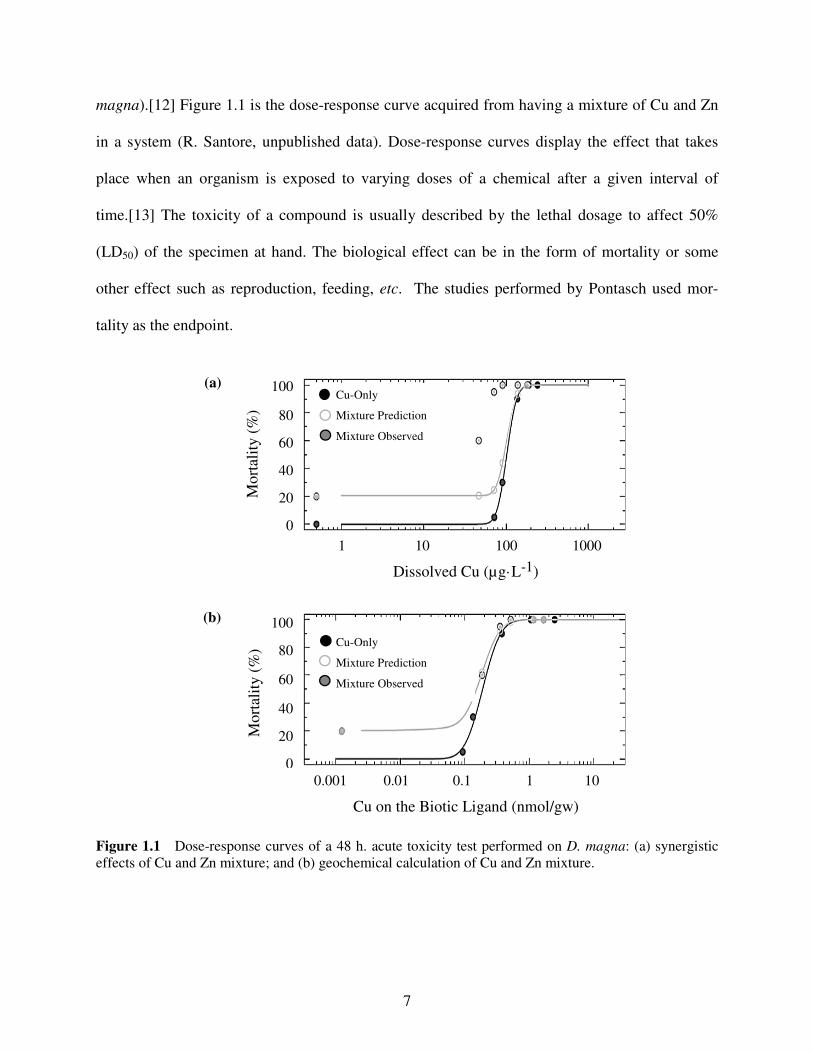
magna).[12] Figure 1.1 is the dose-response curve acquired from having a mixture of Cu and Zn
in a system (R. Santore, unpublished data). Dose-response curves display the effect that takes
place when an organism is exposed to varying doses of a chemical after a given interval of
time.[13] The toxicity of a compound is usually described by the lethal dosage to affect 50%
(LD50) of the specimen at hand. The biological effect can be in the form of mortality or some
other effect such as reproduction, feeding, etc. The studies performed by Pontasch used mor-
tality as the endpoint.
Figure 1.1 Dose-response curves of a 48 h. acute toxicity test performed on D. magna: (a) synergistic
effects of Cu and Zn mixture; and (b) geochemical calculation of Cu and Zn mixture.
(b)
(a)
Cu-Only
Mixture Prediction
Mixture Observed
Dissolved Cu (µg·L-1)
Cu on the Biotic Ligand (nmol/gw)
Cu-Only
Mixture Prediction
Mixture Observed
Dissolved Cu (µg·L-1)
Cu on the Biotic Ligand (nmol/gw)
1 10 100 1000
Cu-Only
Mixture Prediction
Mixture Observed
0.001 0.01 0.1 1 10
100
80
60
40
20
0
Mort
alit
y (
%)
100
80
60
40
20
0
Mort
alit
y (
%)

8
The experiment illustrated in Figure 1.1 used a constant Zn concentration equal to 330
µg·L-1
. This concentration is the value determined to yield approximately 20% mortality in the
D. magna in a Zn-only exposure and was used to confirm Zn was in solution. The test solution
was Environmental Protection Agency (EPA) moderately hard laboratory water, which also
contained 3 mg·L-1
dissolved organic carbon (6 mg·L-1
International Humic Substances Society
Suwannee River fulvic acid). While the Zn concentration was held constant, varying concen-
trations of Cu were added into the system. Percent mortality of the D. magna is shown plotted
against dissolved Cu in Figure 1.1(a). The Cu-only dose-response curve is represented by the
solid black circles. Probit analysis of the data is shown as a solid line, which displays an LD50 of
about 100 µg·L-1
. The actual observed toxicity in the Cu and Zn mixture is shown as the solid
grey circles. Predicted toxicity is represented by the open symbols and its probit line.
The prediction of the Cu and Zn mixture dose-response curve comes from the assumption
that two metals in a system will lend a response that is the sum of the two individual dose-
response curves (i.e. additive behavior). When the Cu and Zn mixture curve are simply added,
the predicted LD50 is 90 µg·L-1
. However, what is actually observed is a much lower LD50
(approximately 50 µg·L-1
) than the additive prediction, demonstrating a synergistic effect.
Figure 1.1(b) shows data from the same toxicity test but with a different data treatment.
In this case, the BLM was used to account for multiple metals competing for complexation with
constituents in the water such as DOC. The model is also able to predict how much of each metal
will bind to the aquatic organism as a biotic ligand. However, competition for binding to the
biotic ligand was not allowed for, due to the lack of data. In essence, the more metal that is
bound to DOC in the water, the less available it is to be bound to the biotic ligand. However, if
more metal cations are present in solution, a higher chance of metals being displaced from the

9
DOC can occur which would then be available to bind to the biotic ligand on the organism. The
BLM computation showed this effect in Figure 1.1(b). The amount of Cu predicted to be
accumulated at the BLM is essentially the same for both the Cu-only and the Cu-Zn mixture
tests. These results are consistent with the central hypothesis of the BLM stating that there exists
a critical metal accumulation level at which mortality occurs (LA50). When geochemical pro-
cesses are taken into account, the predicted dose-response curve of the Cu and Zn mixture
correlates well to the actual observed data.
1.3 Hypothesis to be Tested
In order to explain the observed synergistic toxic effects of Cu and Zn on the tested
species, D. magna, a hypothesis was formulated that Zn, at levels on the order of a few hundred
µg·L-1
, can displace Cu from the fulvic acid. BLM modeling provided by HydroQual
(environmental consulting firm, Mahwah, New Jersey) supported this hypothesis, which was
shown in Figure 1.1(b). As part of the work reported in this thesis, another model, Visual
MINTEQ, was applied to further examine the speciation of Cu and Zn in the test media. The
results from the model data in conjunction with the previous toxicity testing data helped set up a
series of experiments to further test the hypothesis using two analytical techniques, namely Cu2+
-
ISE and Fl FFF-ICP-MS. The work presented in this thesis gives insight on multi-metal
competition of trace metals in natural waters. By understanding the competitive interactions of
Cu2+
and Zn2+
, an understanding of their inherent ecotoxicity can be predicted and effective ways
to remediate these metals can be proposed.

10
1.4 Natural Organic Matter
Natural organic matter (NOM) is used to describe material resulting from the decom-
position of biomass. NOM in ocean water differs greatly than that from coastal or fresh waters.
In open marine waters, organic matter is considered mainly autochthonous since it is produced
within the water body.[14] Conversely, shoreline areas and fresh water has mostly allochthonous
NOM, which is introduced into the water from the surrounding soils, primarily from the
decomposition of terrigenous plants.[15],[16] Typically, terrigenous organic matter is composed
of 50% carbon by weight.[17] Therefore, solutions made with 6 mg·L-1
of NOM should have
approximately 3 mg·L-1
DOC present. Because not all biomass is generated from a single
biological source, it is difficult to classify NOM. The humic fraction portion of NOM can be
generalized as humic substances.
Humic substances are a heterogeneous group of molecular organic molecules that are
ubiquitous in the environment and easily form complexes with metals such as Cu2+
and Zn2+
.[18]
Three broad operationally-defined classes are used to describe humic substances: fulvic acid
(FA), humic acid (HA), and humin. FAs are yellow to tan in color, have a low molecular weight
of 0.5 to 2.0 kDa, and are soluble across the entire pH range. HAs are tan to brown in color, 1 to
10 kDa, and are soluble at a pH greater than 2. Finally, humin is black in color, exhibits quite
large molecular weights (usually ≤300 kDa), and is insoluble at all pHs.[18],[19]
Specific to this work, Suwannee River fulvic acid (SRFA) was the sole humic substance
used in complexation modeling and experiments. The reason for using SRFA is three-fold. First,
FA comprises the largest concentration of all humic substances in natural waters.[19] Second,
SRFA is a reference material from the International Humic Substances Society (IHSS) and it is

11
easy to obtain the freeze-dried standard. Finally, SRFA has been studied by numerous authors
and is well-characterized.
1.4.1 Metal Complexation to Natural Organic Matter
Complexation of Cu or Zn by natural organic matter (NOM) can significantly lower the
free Cu2+
and Zn2+
activity relative to the total dissolved metal, thus allowing for only a
miniscule fraction to be free Cu or Zn. Even though the fraction of Cu and Zn can be quite low in
aquatic systems, the bioavailability of this free metal to aquatic biota can still result in aquatic
toxicity.[20] In order to gauge the level of toxicity in aquatic systems, an understanding of the
binding of metals by NOM is necessary and is the focus of this work.
Humic substances have many groups capable of deprotonating that are available for both
monodentate and bidentate ligand binding (M-L and M-L2) and also have the capacity for cation
exchange, allowing for metal-NOM complexation. Various functional groups can be found in
NOM. The most abundant are the oxygen (O) containing functional groups of carboxylics
(COOHs) and phenolics (OHs).[21],[22] Less abundant functional groups, including amines
(RNH2) and thiols (RSH), can also have an important role in complexation, but little is known
about these groups.[21] The functional groups in humic substances behave as acids and
dissociate at pH values characteristic of the respective group’s acidity constants. The pKa values
for the major functional groups vary. Carboxyls have a pKa between 4—6, phenols are between
9—11, and amines and thiols range between 8.5—12.5. More on this topic, as well as a
hypothetical structure of a humic substance, can be found in Section 2.2.1.

12
1.5 Geochemical Methods to Analyze Metal Complexes
Through the use of geochemical modeling, major aqueous complexes of Cu and Zn can
be simulated under the toxicity testing conditions of the D. magna experiments. By modeling
these conditions, both the organic- and inorganic-Cu complexes can be analyzed to determine if
significant release of Cu2+
is occurring with the addition of Zn. Since the D. magna toxicity tests
suggest that Zn2+
could be competing with Cu2+
for binding sites on the DOC, modeling can
specify concentrations and conditions needed for competition, assuming there are limited binding
sites available to the metal cations.
1.6 Analytical Techniques to Analyze Metal Complexes
Various analytical techniques have been utilized for characterizing metal complexation.
These methods include: anodic stripping voltammetry; field-flow fractionation (FFF) and size
exclusion chromatography, both with inductively coupled plasma-mass spectrometry detection
(ICP-MS); and ion selective electrodes (ISE). The analytical technique chosen should be a
reflection on the sample and its necessary matrix, as well as a consideration of the characteristics
being analyzed. For example, molecular weight distributions of metal complexes can be
determined using Fl FFF-ICP-MS.
In this study, a cupric-ion selective electrode (Cu2+
-ISE) and a flow field-flow fraction-
ator (Fl FFF) coupled to an ICP-MS were the two analytical approaches used to observe metal-
fulvate complexes. The Cu2+
-ISE was chosen as it is a robust technique and has been well-
established in regards to environmental samples. Fl FFF-ICP-MS was selected as the Fl FFF
offers superb molecular weight separation that does not harm the sample and the ICP-MS can
determine metals present in the ppt range.

13
1.6.1 Cupric-Ion Selective Electrode
Cupric-ion selective electrodes (Cu2+
-ISE) have been described in the literature to
successfully measure the complexation of NOM with cupric ions, without any pretreatment.[23]
With respect to humic substances, it is opportune to not pretreat samples as they are prone to
decarboxylation and oxidation and can also sorb with any of the chemicals used in the pretreat-
ment process.[24],[25] A comprehensive analysis of Cu2+
-ISE is detailed in Chapter 3.
1.6.2 Flow Field-Flow Fractionation with Inductively Coupled Plasma-Mass Spectrome-
try Detection
A flow field-flow fractionator (Fl FFF) is traditionally equipped with an ultraviolet (UV)
absorbance detector when determining environmental samples because the organic molecules
present in the sample can be characterized with the proper UV filter. However, the detector(s)
used are dependent on the requirements of the sample and the type of analysis that is to be
achieved. Addition of ICP-MS as a detector allows for the investigation of the molecular weight
distribution of metal complexes.
The main attribute of an FFF is that separation can be achieved without harming the
sample being measured. Polydispersed samples, like those of many environmental samples, are
best characterized if separated so that only simple fragments are introduced for chemical
analysis.[26] FFF is able to separate samples very quickly and selectively as it can be focused on
different working size ranges by changing various parameters, such as its flow rate or carrier
fluid matrix.[26] One of the best attributes of FFF is its ability to easily couple to other
instruments. For this work, the hyphenation of an Fl FFF to inductively coupled plasma with
mass spectrometry detection (ICP-MS) was used. This coupling allows for superior separation by
14
the Fl FFF while also being able to quantify metals at the ppt range by the ICP-MS. A more
detailed description on Fl FFF-ICP-MS is given in Chapter 4.
1.7 Thesis Organization
This chapter was meant to introduce Cu and Zn by demonstrating their significance as
metals that are both physically and physiologically important. Mixtures of Cu and Zn have
shown a more-than-additive toxicological effect on the tested specimen, D. magna. To under-
stand this synergy, a series of geochemical models were utilized to determine if significant
freeing of Cu from the organic matter is occurring with the addition of Zn. This work is detailed
in Chapter 2. Since theoretical data is not enough to explain toxicity testing data alone, two
analytical approaches were taken. The first was the Cu2+
-ISE which quantitatively observed Cu2+
and its fluxes from the addition of a Zn salt, with the results being presented in Chapter 3. The
second analytical approach presents the qualitative results of the complexation of Cu and Zn with
SRFA using Fl FFF-ICP-MS. These results are shown in Chapter 4. Finally, Chapter 5
summarizes the main points of each chapter and concludes the thesis.

15
CHAPTER 2
MODELING APPROACHES
2.1 Introduction
Cu and Zn are essential trace metal nutrients necessary for the survival of aquatic biota.
However, when the biological requirements are exceeded, Cu and Zn can become toxic to these
organisms. Elevated levels of Cu and Zn come from anthropogenic activities, primarily mining,
farming, industrial activities and municipal or industrial wastewaters that release metals into the
water system.[27] Because metals can sorb to particles and sediments in waterways, the analysis
of sediment cores can give historical trends in metal concentrations. These cores have
demonstrated that there has been an increase of Cu and Zn in sediments over the past few
decades.[28],[29] The continual upward trend of Cu and Zn being present in waters raises
concern for not only the health of aquatic biota but also that of humans as well.
The divalent species of Cu and Zn (Cu2+
and Zn2+
) are particularly important as they can
be the most toxic. Aquatic organisms are especially harmed by Cu2+
and Zn2+
as they affect their
ionic regulatory systems. In an effort to identify the bioavailability and the environmental fate
and transport of these divalent species to assess the threat they pose to aquatic life, their chemical
speciation needs to be identified.[30] Trace metals like Cu and Zn can exist as many aqueous
species, with the toxicity of these metals being more of a function of their ion activity of the free
ion and less of a function of total metal concentration. Often, speciation of trace metals like Cu
and Zn are dominated by complexes containing humic substances.[31],[33] Because not all
species are easily measured by an analytical method and the environmental concentrations of

16
metals are often too low for analytical techniques, geochemical computational models are
utilized.[30]
2.2 Chemical Speciation Modeling
The speciation of dissolved metals in natural waters can be determined through the use of
geochemical computational modeling.[30],[33],[34] Specific to this project, a Windows free-
ware program, Visual MINTEQ (version 3.0, 2012, KTH Royal Institute of Technology,
Stockholm, Sweden), was utilized. The model can account for various components of natural
waters such as alkalinity (Alk), concentration of the water constituents (metals, natural organic
matter, and salts), pH and temperature. National Institute of Standards and Technology critical
stability constants are the majority of the complexation constants used in the Visual MINTEQ
database.[35]
Table 2.1 Laboratory water composition input into Visual MINTEQ based on toxicity test constituents.
Constituent Concentration (mg·L-1
)
Cl- 1.8
K+ 1.8
Mg2+
12.5
Ca2+
13.5
Na+ 24.0
SO42-
90.0
Alkalinity (mg CaCO3·L-1
) 55.0
Examining a modeling approach described as “Simulated Freshwater” encompasses the
bulk of this chapter. The model set used for the Simulated Freshwater components consist of pH,
DOC values, and metal concentrations that are synonymous with those commonly found in rivers
and streams. This approach has moderately hard water (MHW) constituents with concentrations
outlined by the EPA.[36] The specific concentrations used can be found in Table 2.1, whereby
the six ions listed are components in MHW. The Alk is reported as milligrams of calcium

17
carbonate per liter of water (mg CaCO3·L-1
). Ion speciation was computed using the database
equilibrium constants in Visual MINTEQ.
2.2.1 Implications of DOC on Metal Speciation Estimated by the SHM
Humic substances greatly affect the binding and transport of trace metals which, in turn,
affects the toxicity and transport of these metals in natural waters. Because terrigenous organic
matter is composed of 50% of carbon by weight, the effects of SRFA on the binding of Cu and
Zn can be modeled by inputting DOC, which is half of the total SRFA concentration in solution.
There are multiple models containing DOC but the one presented here is the Stockholm Humic
Model (SHM) because of its known success in accurately describing metal and DOC
complexation. Much of the success of the SHM is due to its ability to predict site heterogeneity
of humic binding sites and apply electrostatic interactions which provides a realistic approach in
predicting ligand interactions.[37]
Figure 2.1 Theorized fulvic acid structure denoting the various positions of carboxylic and phenolic
groups (adapted from MacCarthy).[18]
Humic substances are heterogeneous in nature and their structure is not well-defined.
Because organic matter differs from region to region, it is difficult to characterize the
decomposed matter. However, it is known that humic substances are generally composed of

18
simple, oxygen-containing functional groups namely: alcohols, carboxyls, hydroxyls, phenols,
and sulfur-containing groups, specifically thiols.[38]-[40] The most important metal binding
functional groups, however, are presumed to be carboxylic and phenolic OHs.[39] These groups
easily deprotonate becoming attractive binding sites for metal cations. However, the positions of
these metal binding groups on the humic substance vary in location. For instance, there are
carboxylic groups off of cyclic ethers and others being on aliphatic chains as shown in Figure
2.1.
The asymmetric distribution of nearby electronegative groups influence the degree of
proton dissociation and affect the metal binding strength.[21],[41] To account for site variability,
the SHM calculates the total amount of proton-dissociating sites of the various groups. The site
density consists of the sum of all the groups, but carboxylic and phenolic groups particularly
comprise most of the density. The SHM denotes carboxylic acid sites as Type A sites and are
considered to be very strong sites with a pKa ranging from 4—6 therefore dominating metal
complexation at pH values less than 7. The phenolic groups, falling in the category of Type B
sites are dominant at pKas ranging from 9—11, thus having dominance at higher pHs. The Type
A and B groups are important to distinguish because some metals preferentially bind to the Type
A strong acid sites which are less abundant whereas other metals bind to Type B sites which are
less acidic but are more dense in the humic substance.[21]
Equation 2.1 shows a generic humic substance functional group () at first being bound
to a proton (). Dissociation yields a negatively charged humic molecule () and a proton
(), which are then both available for binding other constituents. The dissociation of this
reactant is determined by the intrinsic dissociation constant ().[21]
↔ + , (2.1)
19
The SHM estimates eight sites on the humic substance in which a metal can bind and are
denoted by Equations 2.2a and 2.2b. Said equations each use fitting parameters to account for
site variability. The first set of sites shown in Equation 2.2a are the Type A groups (strong acid
sites) and are mostly attributed to the carboxylic groups. The second sites denoted in Equation
2.2b are meant to represent the Type B groups (weak acid sites) which are assigned primarily to
phenolic groups. The values do not necessarily describe discrete sites but rather serve as a
vehicle for the SHM to describe the inherent variability in humic substances’ acid-base equil-
ibria.[21]
= 1 − 4: = −()
∆ (2.2a)
= 5 − 8: = !"#$% −(&')
∆ !"#$% (2.2b)
Along with understanding the acid dissociation, it is also important to account for binding
interactions and site heterogeneity. Cu and Zn can either bind to humic substances via
monodentate or bidentate chelation. Although Equations 2.3—2.6 use Cu as an example, the
same equations can also be applied for Zn. Equation 2.3 predicts the reaction stability for the
monodentate interaction of Cu. Here, Cu2+
is bound to the humic substance () at one of the
monodentate sites, leaving the complex with a positive charge. The mondentate Cu interaction is
described by its intrinsic binding constant (()*).[21]
+,+ ↔ H + +,, ()* (2.3)
()* must account for the heterogeneity of sites on the humic substance so it is adjusted
with a heterogeneous metal fitting parameter (∆.) as shown in Equation 2.4. Fulvic acid has
varying binding strengths of carboxylic and phenolic groups since the location of the group on
the humic substance varies which was displayed in Figure 2.1. As such, a distribution term

20
(∆.) is meant to account for the variability of complexation sites and has four sub-sites of
differing metal-humic complexation affinity.[21]
()*,/ = ()* + 0 ∙ ∆., 0 = 0, 1, 2, 3 (2.4)
The other type of metal binding is via bidentate chelation where there are two sites on the
same humic substance that binds Cu or Zn. Equation 2.5 predicts the reaction stability for the
bidentate interaction of the metal, where Cu2+
is bound to the humic substance () at two sites,
yielding a neutral complex. The bidentate Cu interaction is described by its intrinsic binding
constant (()5).[21]
+,$+2 ↔ 2H + +,, ()5 (2.5)
Again, there is a heterogeneity fitting term that is associated with the metal’s intrinsic
binding constant. The only difference between Equation 2.4 and Equation 2.6 is that the
bidentate calculation has a heterogeneity term that is doubled to account for each site of action.
()5,/ = ()5 + 20 ∙ ∆., 0 = 0, 1, 2, 3 (2.6)
2.3 Visual MINTEQ Modeling for Simulated Freshwater
The exact concentrations used for the Simulated Freshwater analyses are equivalent to the
concentrations used in the toxicity tests for D. magna. The inputs consisted of the MHW
constituents listed in Table 2.1, pH equal to 8.35, and varying concentrations of Cu, Zn, or both
metals together, typically in the µg·L-1
range. By modeling the conditions that the D. magna
incur during the toxicity tests, the activity coefficients of Cu and Zn and their competition for
binding sites on the DOC can be determined.

21
2.3.1 Cu Complexes in Simulated MHW
Visual MINTEQ was used to model the log activity of various important Cu complexes
as a function of the log of the total Cu (CuT) placed into the simulation EPA MHW and is shown
in Figure 2.2(a). The input Cu concentrations were 1 µg·L-1
to 1 mg·L-1
. Without any organic
matter present, a constantly linear relationship exists between the increasing Cu and its
associated inorganic Cu complexes.
Figure 2.2 Effects on major aqueous Cu complexes in simulated EPA MHW modeled in Visual
MINTEQ when: (a) [Cu] varies from 1 µg·L-1
to 1 mg·L-1
at pH = 8.35; and (b) [Cu] = 100 µg·L-1
and pH
varies from 2 to 9.
(a)
(b)

22
The most abundant constituent is Cu carbonate (CuCO30
(aq)) which would be expected
because carbonates readily form due to the dissolving of carbon dioxide (CO2) from the
atmosphere into the water. Also, the modeled pH was 8.35, which is relatively close to the CO32-
pKa of 10.3. Free copper (Cu2+
) is predicted to be approximately two orders of magnitude lower
in concentration than the most abundant species, CuCO30
(aq).
In Figure 2.2(b), Cu concentrations were held constant at 100 µg·L-1
and pH values were
varied from 2 to 9 to better understand the major complexes that form in EPA MHW. The Cu
concentration of 100 µg·L-1
was chosen as this was the LD50 of the D. magna during the acute
toxicity tests. At lower pHs, Cu2+
is the dominant species until the pH reaches approximately 6.
At higher pH values, the species CuCO30
(aq) becomes dominant, which agrees with the findings
in Figure 2.2(a).
2.3.2 Cu-Organic Complexes in Simulated MHW
Before modeling the behavior of Cu when Zn is present in waters with organic matter, a
model of how Cu behaves in EPA MHW with DOC present was assessed using Visual
MINTEQ. Figure 2.3(a) displays the log activity of various important Cu complexes as a
function of the log of the total Cu (CuT) placed into the simulated EPA MHW with 6 ppm
SRFA (3 mg·L-1
DOC). The two dominating species are the bidentate Cu-FA species (FA2Cu)
and the cuprous-FA hydroxide species (FA2CuOH(aq)) until after about 1.0·10-5
M and 5.8·10-6
M, or 650 µg·L-1 and 370 µg·L
-1, respectively of Cu is added. At this juncture, the FA2Cu and
FA2CuOH(aq) complexes are secondary to the CuCO30
(aq) complex. This is important because
when Cu is the only metal present, the organic complexes become less prominent after
approximately 370 µg·L-1
has been placed into the water, while many of the inorganic complexes
are rapidly increasing.

23
Figure 2.3 Effects on major aqueous Cu complexes in simulated EPA MHW with DOC modeled in
Visual MINTEQ when: (a) [Cu] varies from µg·L-1
to 1 mg·L-1
at pH = 8.35; and (b) [Cu] = 100 µg·L-1
and pH varies from 4 to 9.
The dominant species from varying the Cu concentrations are similar to those species
present when varying the pH from 4 to 9. In Figure 2.3(b), Cu concentrations were held constant
at 100 µg·L-1
while the pH was varied. Again, 100 µg·L-1
Cu was chosen since this is the
approximate LD50 of D. magna. Similar to Figure 2.3(a), the major complexes that form in EPA
MHW with DOC present is FA2Cu until the pH equals 8 at which point FA2CuOH(aq) becomes
the dominant species. It is important to note that under these conditions, Figure 2.3(b)
(a)
(b)

24
demonstrates that the Cu2+
species is orders of magnitude lower than many of the other
complexes. Since most of the toxicity data occurs at a pH of approximately 8.35, it is important
to note that the predicted Cu2+
activity at this pH is 5.0·10-9
M.
2.3.3 Organic Complexes in Simulated Freshwater
Figure 2.4 displays log activity of various important organic complexes as a function of
the log of the total Zn (ZnT) placed into the system. EPA MHW with 6 ppm SRFA (3 mg·L-1
DOC) was modeled in Visual MINTEQ. Into the simulated solution, a Cu concentration of 100
µg·L-1
was added and held constant while Zn concentrations were varied from 10 µg·L-1
to 1
mg·L-1
. The Cu concentration of 100 µg·L-1
is the approximate LD50 of the D. magna determined
by acute toxicity tests. By sweeping the Zn concentration in this simulation, the concentration at
which bound Cu begins to be freed can be determined.
Figure 2.4 Effects on major aqueous Cu complexes in simulated EPA MHW with DOC modeled in
Visual MINTEQ with 3 mg·L-1 DOC, pH = 8.35, [Cu]T = 100 µg·L
-1, and [Zn]T varying from 10 µg·L
-1
to 1 mg·L-1
.

25
The model displays a significant increase in Cu2+
occurring when approximately 1.5·10-6
M, or about 100 µg·L-1
, of Zn is added into the system. As expected, a similar upward trend is
noticed at the same concentration for monodentate binding of Cu and fulvic acid (FACu+). These
two curves, shown in Figure 2.4, are zoomed in and displayed in Figure 2.5(a) in order to better
perceive the increase. As the FACu+
ligand increases, there appears to only be a slight decrease
in the bidentate Cu and fulvic acid (FA2Cu) complex as seen in Figure 2.5(b). However, since
the concentration of the FA2Cu complex is nearly two orders of magnitude higher in activity than
that of the FACu+
ligand, this decrease is actually quite significant. When the FA2Cu complex
dissociates into one FA molecule with two available binding ligands and one Cu2+
, a total of
2·10-8
Cu2+
dissociates into the solution. The released bidentate FA is complexing with Cu in the
monodentate form and also with Zn in both monodentate (FAZn+) and bidentate (FA2Zn)
complexes. Of the 2·10-8
Cu2+
that becomes displaced overall, 1.2·10
-9 of the ion binds as the
FACu+
complex and 8·10-10
is freed as Cu2+
. This corresponds to 2·10-9
, or 10%, of the 2·10-8
Cu2+
displaced from the FA2Cu complex, leaving 1.8·10-8
of Cu2+
unaccounted for. Therefore, it
appears that there is more Cu2+
than what is getting freed from the Cu-FA complexes, suggesting
that not 100% of all the Cu is bound to the NOM. By way of viewing the raw data values, nearly
all of the Cu2+
that becomes free from FA complexation forms inorganic complexes in the EPA
MHW.
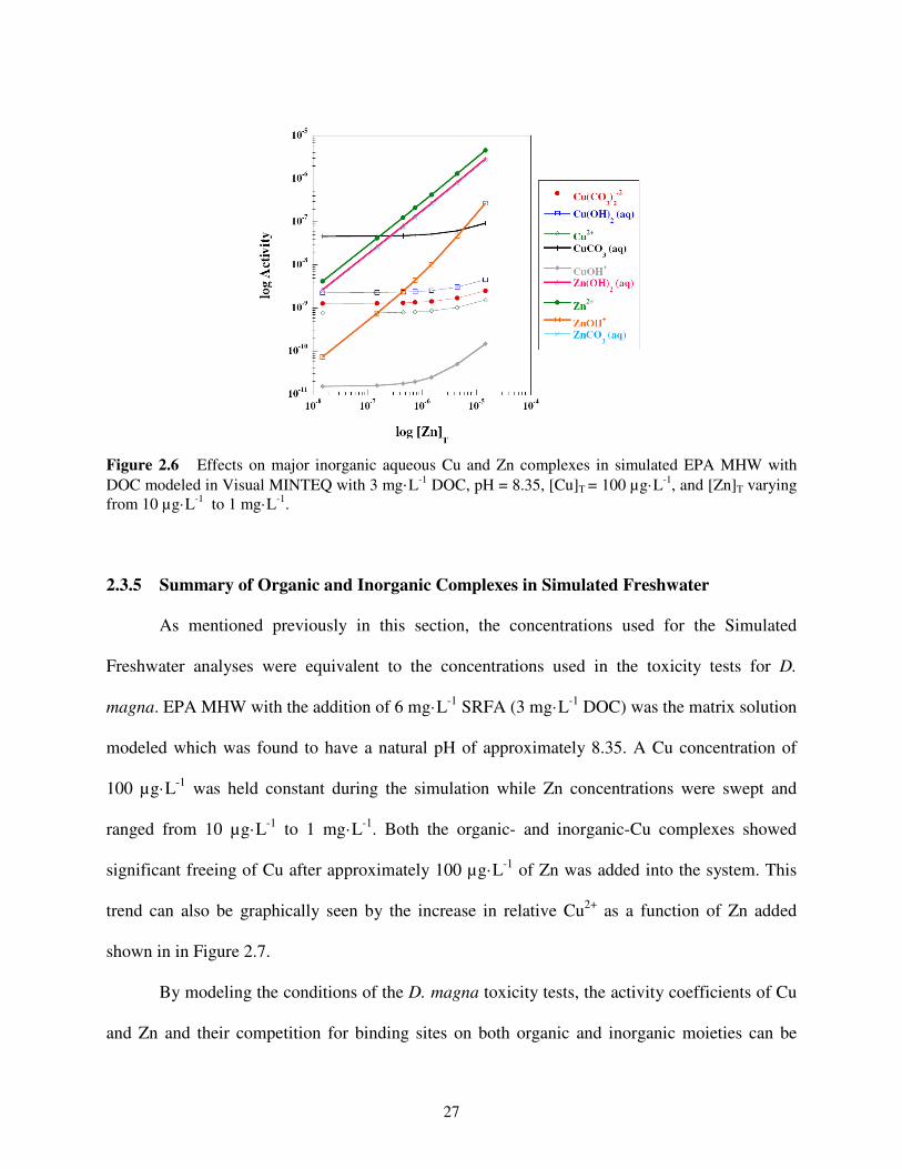
2.3.4 Inorganic Complexes in Simulated Freshwater
The log activity of the important inorganic complexes as a function of the log of the total
Zn (ZnT) placed into the system was also modeled using Visual MINTEQ and is shown in Figure
2.6. Again, EPA MHW with 6 mg·L-1
SRFA (3 mg·L-1
DOC) was the matrix modeled to observe

26
the effects of Cu and Zn competition. Into the simulated solution, a Cu concentration of 100
µg·L-1
was added and held constant while Zn concentrations were swept and ranged from 10
µg·L-1
to 1 mg·L-1
. For consistency, the pH was held constant at 8.35 and 100 µg·L-1
of Cu was
chosen since this was the approximate LD50 of the D. magna. By sweeping the Zn concentration
in this simulation, the concentration at which bound Cu begins to be freed can be determined.
Figure 2.5 Effects on FA-Cu and Cu2+
with increasing Zn concentration in EPA MHW with DOC
modeled in Visual MINTEQ with 3 mg·L-1 DOC, pH = 8.35, [Cu]T = 100 µg·L
-1, and [Zn]T varying from
10 µg·L-1
to 1 mg·L-1
, with: (a) zoomed in to show the increasing trend of FACu+ and Cu
2+; and (b)
zoomed in to show the decreasing trend of FA2Cu.
Similar to the organic complexes, the first modeled point displaying a significant increase
in free Cu2+
occurs when approximately 1.5·10-6
M, or about 100 µg·L-1
, of Zn is added into the
system. This same Zn concentration also causes an upward trend for all of the Cu-inorganic
complexes displayed in Figure 2.6. As would be expected, a linear relationship exists between
the Zn activity and the total Zn being added. Likewise, the carbonate and hydroxide complexes
with Zn are also linear, displaying a direct relationship between the Zn added and its appropriate
complex that is formed.
(a) (b)
27
Figure 2.6 Effects on major inorganic aqueous Cu and Zn complexes in simulated EPA MHW with
DOC modeled in Visual MINTEQ with 3 mg·L-1 DOC, pH = 8.35, [Cu]T = 100 µg·L
-1, and [Zn]T varying
from 10 µg·L-1
to 1 mg·L-1
.
2.3.5 Summary of Organic and Inorganic Complexes in Simulated Freshwater
As mentioned previously in this section, the concentrations used for the Simulated
Freshwater analyses were equivalent to the concentrations used in the toxicity tests for D.
magna. EPA MHW with the addition of 6 mg·L-1
SRFA (3 mg·L-1
DOC) was the matrix solution
modeled which was found to have a natural pH of approximately 8.35. A Cu concentration of
100 µg·L-1
was held constant during the simulation while Zn concentrations were swept and
ranged from 10 µg·L-1
to 1 mg·L-1
. Both the organic- and inorganic-Cu complexes showed
significant freeing of Cu after approximately 100 µg·L-1
of Zn was added into the system. This
trend can also be graphically seen by the increase in relative Cu2+
as a function of Zn added
shown in in Figure 2.7.
By modeling the conditions of the D. magna toxicity tests, the activity coefficients of Cu
and Zn and their competition for binding sites on both organic and inorganic moieties can be

28
evaluated. Typically, NOM in natural waters dominates the speciation of the metals present so a
more in-depth approach in determining the role of the fulvic acid and, consequently, the effect of
Cu and Zn binding to DOC was taken and compared to the inorganic complexes.
Figure 2.7 Effects on free Cu2+
with increasing [Zn] relative to 1 µg·L-1
Zn in EPA MHW modeled in
Visual MINTEQ.
Table 2.2 displays the total Zn added and the correlating summed molar values of the
organic as well as the inorganic complexes that form with Cu. The final column presents the free
Cu2+
concentration that is estimated by the model. The Cu-organic complexes are shown to
decrease with the addition of Zn while the Cu-inorganic complex concentrations are increasing.
Based on these values, it is clear to see that as more Zn is being added into the system, more Cu
is becoming unbound denoted by the Cu2+
values increasing. Though the amount of Cu2+
is
subtle, it agrees with the hypothesis of Zn displacing Cu. According to the data shown in Table
2.2, most of all bound Cu is to the NOM since the Cu organic complexes show a whole order of
magnitude higher concentration than the Cu-inorganic complexes.

29
Table 2.2 Effect of increasing [Zn]T to the sum of the Cu-organic and Cu-inorganic complexes.
[Zn]T (M) Σ Cu-Organic
Complexes (M)
Σ Cu-Inorganics
Complexes (M) Free Cu
2+ (M) CuT (M)
1.53•10-8 1.50•10-6
5.58•10-8 7.75•10-10
1.56•10-6
1.53•10-7 1.50•10-6
5.65•10-8 7.84•10-10
1.56•10-6
4.59•10-7 1.50•10-6
5.78•10-8 8.03•10-10
1.56•10-6
7.64•10-7 1.50•10-6
5.92•10-8 8.22•10-10
1.56•10-6
1.53•10-6 1.50•10-6
6.25•10-8 8.69•10-10
1.56•10-6
4.59•10-6 1.48•10-6
7.50•10-8 1.04•10-9
1.56•10-6
1.53•10-5 1.44•10-6
1.12•10-7 1.56•10-9
1.56•10-6
2.4 Toxicity Modeling
Other models not only account for speciation but also consider water quality standards
and toxicity to aquatic organisms in order to calculate toxicity over a range of environmental
conditions.[3] An important aspect of this type of model is the ability to assess dose-response
relationships. Single metal toxicity has been an area heavily investigated, but there is currently a
knowledge gap when considering how multiple metals compete with one another.
Modeling in Visual MINTEQ suggests that when Cu and Zn metals are competing for
binding sites, whether on the aquatic organism itself or on an inorganic or organic constituent, a
synergistic effect often occurs. In an effort to understand the modeling’s outputs and partially fill
the knowledge gaps existing with multi-metal competition especially in regards to DOC binding,
analytical techniques were employed and are described in this thesis.
2.5 Conclusions
Major aqueous complexes of Cu and Zn were determined by simulating the toxicity
testing conditions of D. magna using Visual MINTEQ. The SHM was chosen for modeling DOC
since it can predict site heterogeneity and, therefore, ligand interactions with metals. To account

30
for site variability, the SHM calculates the total amount of proton-dissociating sites of the
various groups, whereby a fitting parameter is employed to estimate the variances of humic
substances’ acid-base equilibria.
Both the organic- and inorganic-Cu complexes showed significant freeing of Cu after
approximately 100 µg·L-1
of Zn was added into the modeled system. Similarly, data from Table
2.2 demonstrates that with the addition of Zn, a decrease in the Cu-Organic complexes occurs.
For instance, when only 1 µg·L-1
of Zn is present in the model, 96% of the CuT remains bound to
the DOC. When 1 mg·L-1
of Zn is present in the model, 92% of the CuT is bound to the DOC.
Based on these values, the theoretical data agrees with the hypothesis, suggesting that Zn2+
is
outcompeting Cu2+
for binding sites on the DOC.

31
CHAPTER 3
CUPRIC-ION SELECTIVE ELECTRODE
3.1 Introduction
The binding of trace metals like Cu and Zn to humic substances controls the chemical
speciation of the metal by forming a complex, essentially lessening the amount of free metal that
is bioavailable that could be toxic to aquatic organisms.[31],[42] The use of ion selective
electrodes (ISEs) to study competition between metals and humic substances has been an area
heavily researched since the late 1980’s. During this time, aquatic geochemistry models were
advancing quickly and much data was required for their operation. Of particular interest were the
known toxic species of Cu and cadmium (Cd). However, most studies were related to the
interference Cu and Cd had on the uptake of other trace metal nutrients, especially in regards to
aluminum (Al3+
), manganese (Mn2+
), iron (Fe3+
), and zinc (Zn2+
).[43]-[49] The competition of
metal ions with hard water constituents such as magnesium ion (Mg2+
) and calcium ion (Ca2+
)
were also thoroughly studied.[50],[51] Similarly, there was focused attention on the complex-
ation of Cu2+
and Cd2+
with fulvic acid because often this binding lessened the toxicity to aquatic
organisms in natural waters.[38],[52],[53] Understanding the behavior of toxic metal ions greatly
allows for predicting ecotoxicity.
Particular to this project, the behavior of Cu and Zn in the presence of fulvic acid is
evaluated. Although there are many studies outlining the complexation of Cu with naturally
occurring organic macromolecules like fulvate, there is very little data existing between the
competitive interactions of Cu and Zn on DOC. There is, however, information on the binding
capacities of Cu2+
and Zn2+
to soil humic acids using fluorescence spectroscopy and literature

32
acknowledging the fact that competitive interactions are seen between Cu2+
and Zn2+
for binding
to cellular ligands.[44],[45],[54]
One way of characterizing a metal that is bound to the DOC in fulvic acid is to determine
the concentration of free ions in solution. This can be done by using an ISE such as the Cu2+
ion
selective electrode (Cu2+
-ISE), where any cupric ions that have been displaced from the DOC
will be detected. Therefore, if a Cu-fulvate complex exists but the introduction of Zn causes Cu
to be displaced, then an increase in Cu2+
should occur and can be detected by the Cu2+
-ISE.
3.2 Cupric-Ion Selective Electrode Theory
Cu2+
-ISEs have been used extensively in the past and are still applicable today. As is
typical with many ISEs, the Cu2+
-ISE has a crystal membrane that probes for one specific ion in
solution; in this case, the cupric ion. When the membrane comes into contact with a Cu2+
, a
potential develops. The potential is measured against a constant reference potential. If more Cu2+
exists in solution then the potential will be higher.
6 = 67 +.'7'9:
#;· (=) (3.1)
The total measured electrode potential of the sensing and reference electrodes (6) is
measured in millivolts (mV) and relates to the concentration of Cu2+
in solution through the
Nernst equation shown in Equation 3.1. The reference potential (67) is a constant value and is
characteristic to the particular ion selective electrode and reference pair. The logarithm of the
activity of the measured ion is denoted as (=). If a plot of 6 is generated as a function of
(=), then the slope of the line will be the value of .'7'9:
#;, where is the gas constant
measured in J·K-1
mol-1
. > denotes the absolute temperature measured in K, ? represents the
number of electrons, and @ is Faraday’s constant measured in Coulombs (C).
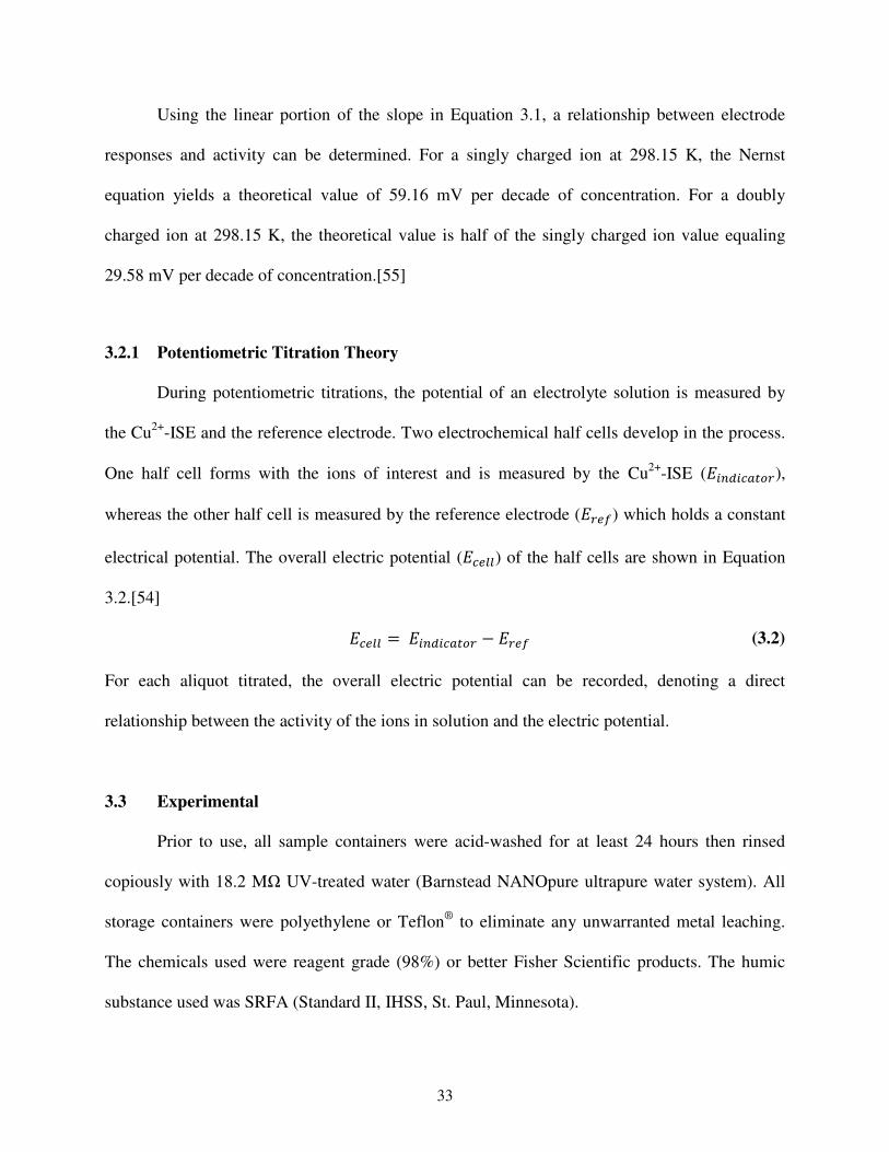
33
Using the linear portion of the slope in Equation 3.1, a relationship between electrode
responses and activity can be determined. For a singly charged ion at 298.15 K, the Nernst
equation yields a theoretical value of 59.16 mV per decade of concentration. For a doubly
charged ion at 298.15 K, the theoretical value is half of the singly charged ion value equaling
29.58 mV per decade of concentration.[55]
3.2.1 Potentiometric Titration Theory
During potentiometric titrations, the potential of an electrolyte solution is measured by
the Cu2+
-ISE and the reference electrode. Two electrochemical half cells develop in the process.
One half cell forms with the ions of interest and is measured by the Cu2+
-ISE (6#ABCD$E),
whereas the other half cell is measured by the reference electrode (6E"F) which holds a constant
electrical potential. The overall electric potential (6B"%%) of the half cells are shown in Equation
3.2.[54]
6B"%% =6#ABCD$E − 6E"F (3.2)
For each aliquot titrated, the overall electric potential can be recorded, denoting a direct
relationship between the activity of the ions in solution and the electric potential.
3.3 Experimental
Prior to use, all sample containers were acid-washed for at least 24 hours then rinsed
copiously with 18.2 MΩ UV-treated water (Barnstead NANOpure ultrapure water system). All
storage containers were polyethylene or Teflon®
to eliminate any unwarranted metal leaching.
The chemicals used were reagent grade (98%) or better Fisher Scientific products. The humic
substance used was SRFA (Standard II, IHSS, St. Paul, Minnesota).

34
3.3.1 Sample Preparation
Concentrated stock solutions of 2·10-1
M copper(II) nitrate (Cu(NO3)2) and zinc(II)
nitrate (Zn(NO3)2) were prepared and then diluted so that final concentrations were 2·10-2
M,
2·10-3
M, and 2·10-4
M. A sub-sample was taken of each stock solution for analysis on
inductively coupled plasma with atomic emission spectrometry (ICP-AES) detection for con-
firmation of the metal concentrations.
All samples were prepared in EPA MHW. The specific concentrations of each constituent
are outlined by the EPA.[36] The Alk was equivalent to 24.5±0.3 mg CaCO3·L-1
when there was
not any NOM in solution and the pH was adjusted to 6.25. However, when the pH was left
unadjusted (~8.35), the Alk was equal to 55.0 mg CaCO3·L-1
. A stock solution of 6 ppm (3
mg·L-1
DOC) of SRFA was prepared in some of the EPA MHW and was used for titrating in
Cu(NO3)2. Another solution containing 2·10-6
M Cu(NO3)2 was made in the 6 ppm SRFA
prepared in EPA MHW and was used for titrating in Zn(NO3)2. The concentrations were
calculated by mass and confirmed by a PerkinElmer ICP-MS (NexION 300 ICP-MS,
PerkinElmer, Waltham, MA, USA).
A stock solution of 6 ppm (3 mg·L-1
DOC) of SRFA was made and used for all of the
analytical experiments for consistency. The concentration was calculated by mass and confirmed
by a Shimadzu total organic carbon (TOC) analyzer (Shimadzu TOC 1000 Carbon Analyzer,
Columbia, MD, USA). These solutions were stored in polyethylene or Teflon®
containers and
were placed in a 4°C refrigerator when not in use to limit any degradation that could occur.
3.3.2 Cupric-Ion Selective Electrode Instrumentation
An Orion Cu2+
double junction ion selective electrode (Cu2+
-ISE) was used for
selectively probing the free Cu2+
in solution. The Cu2+
-ISE was placed in a Teflon®
stopper with

35
three holes atop. One of these holes was for the Cu2+
selective probe (Orion, model 942900),
another hole was for the reference electrode (Orion, model 900200) and the final hole was for the
pH probe. The probes were connected to a Thermo Orion2 Star digital pH/millivolt/temperature
meter. Prior to use, the Cu2+
-ISE was cleaned and filling solution was replaced if needed.
Periodically, the Cu2+
selective probe would be resurfaced by polishing the probe. Because
sunlight altered the Cu2+
-ISE reading, the instrument was placed in a location away from direct
exposure.[23]
3.3.3 Acquiring a Nernstian Response
Prior to each experiment, the electrode was calibrated using a 0.1 M potassium nitrate
(KNO3) background electrolyte that was pH adjusted to 4 in order to eliminate Cu complexation
with hydroxides, carbonates, and fulvates which occur at pH values greater than 5.5. Aliquots of
2·10-2
M Cu(NO3)2 were placed into solution until a total volume of 2 mLs were added. For each
sample, a pH reading was taken at room temperature.
Figure 3.1 Calibration plot displaying Nernstian response of the Cu2+
-ISE using Cu(NO3)2 at pH of 4.

36
The total mV change can be determined and used for reconciling if proper functioning of
the Cu2+
-ISE is occurring. In all of the calibrations, the Nernstian slope was found to be 29.5±1.0
mV, which was in good agreement with the Nernst equation which predicts an exact value of
29.58 mV for a divalent cation. A typical experimental Nernstian graph is shown in Figure 3.1,
whereby mV readings are plotted as a function of log10 concentration.
3.3.4 Copper Titrations
Once the Cu2+
-ISE was calibrated and giving a Nernstian response, both of the probes
were soaked in a 0.025 M sulfuric acid (H2SO4) solution for approximately 30 minutes in order
to rid the selective electrode of any cupric ions on the membrane. Once the response was static,
the electrodes were considered to be conditioned and ready for measurements.
Potentiometric titrations were performed by placing aliquots of the 2·10-4
M to 2·10-1
M
Cu(NO3)2 stock solutions into either EPA MHW by itself or into the 6 ppm (3 mg·L-1
DOC)
SRFA solution. The pHs of the starting solutions was that of the EPA MHW itself which ranged
between 8.1 and 8.3. Additional titrations were performed in solutions that were adjusted to a pH
of 6.25 for comparison of organic to inorganic complexes.
3.3.5 Zinc Titrations
Similar to the Cu titrations, the Cu2+
-ISE was calibrated to assure the electrodes were
giving a Nernstian response. Once this was achieved, both of the probes were soaked in a 0.025
M sulfuric acid (H2SO4) solution for approximately 30 minutes to eliminate any cupric ions that
could be on the membrane of the selective electrode. Once the response was giving a static
reading, the electrodes were considered to be conditioned and ready for measurements.

37
Potentiometric titrations were performed by placing aliquots of the 2·10-4
M to 2·10-1
M
Zn(NO3)2 stock solutions into a solution of 6 ppm (3 mg·L-1
DOC) SRFA prepared in EPA
MHW with a 2·10-6
M Cu(NO3)2 or 2·10-5
M Cu(NO3)2 concentration. Again, the pHs of the
solutions prior to titrating was that of the EPA MHW itself which ranged between 8.1 and 8.3.
Additional titrations were performed in a solution that was adjusted to a pH of 6.25 for
comparison of organic to inorganic complexes.
3.4 Results and Discussion
The data presented here reflects that of the experimental data as well as the computational
values gained from modeling the experimental conditions in Visual MINTEQ. The model was
used to compute Cu and Zn complexes based on the toxicity test aquatic conditions. The effect of
aquatic fulvic acid, inorganic complexation, and competitive binding with other trace elements,
like that of the hard water constituents of Ca2+
and Mg2+
, with Cu and Zn was modeled to
compare against the experimental data.
In the case of the experimental data, each titration was performed at least in duplicate and
at times in triplicate. The error bars represent twice the standard deviation. At very low Cu
concentrations, the Cu2+
-ISE was not able to properly detect the Cu2+
ions in solution since it was
at its lower limit of sensitivity. This is shown by some of the early points in the titration curve
showing little increase in mV as Cu2+
is added and cannot be used to accurately describe the free
Cu2+
in solution. In these cases, the error bars are either non-existent or demonstrate small error
since the Cu2+
-ISE is not detecting specific ions in solution but rather just giving a reading for
the potential of the inert electrolyte in solution. Once the Cu2+
-ISE begins to detect Cu2+
, the
error bars are larger in the lower concentrations and then demonstrate less error at high

38
concentrations. This is expected since at higher concentrations, the Cu2+
-ISE is sensing Cu2+
that
is more in its detection range.
In all of the titration graphs, the Nernst slope has a y-intercept of 10-8
and extends upward
following a straight line. The bound Cu was that which deviated below the Nernstian slope.
Because the pH of the electrolyte solution was adjusted to 4 when performing the Nernstian
response of the Cu2+
-ISE electrode, it is assumed that any Cu(NO3)2 added will be uncomplexed,
free Cu2+
since the pH is below the range of both inorganic and organic complexation. This was
also shown previously in Figure 2.2(b).
3.4.1 Cu Titration of EPA MHW without DOC
The results of Cu(NO3)2 being titrated into EPA MHW without any DOC present is
shown in Figure 3.2. The effect of EPA MHW constituents on the binding of Cu is demon-
strated. Free cupric ions (log free [Cu2+
]) extrapolated from the Cu2+
-electrode are plotted
against the total copper (CuT) of the system. The blue straight line denotes the Nernstian slope
and the red dots represent the actual data given from the Cu2+
-electrode.
Inorganic complexation with the major components of carbonates and hydroxides
generally occur at pH values above 6.3 and 8.0, respectively. Therefore, by adjusting the pH to
6.25, most of the binding can be attributed to Alk constituents. However, adjusting the pH of the
solution also adjusts the Alk of the system. Alk tests revealed that the EPA MHW at a pH of 6.25
has an Alk equal to 24.5±0.3 mg of CaCO3·L-1
. Unadjusted EPA MHW, however, is approx-
imately twice the Alk of the adjusted EPA MHW with an Alk equal to 55.0 mg of CaCO3·L-1
.
When the pH is unadjusted and remains the natural pH of the EPA MHW, significant binding of
the cupric ion occurs which is shown in Figure 3.2(b). For a direct comparison to the toxicity
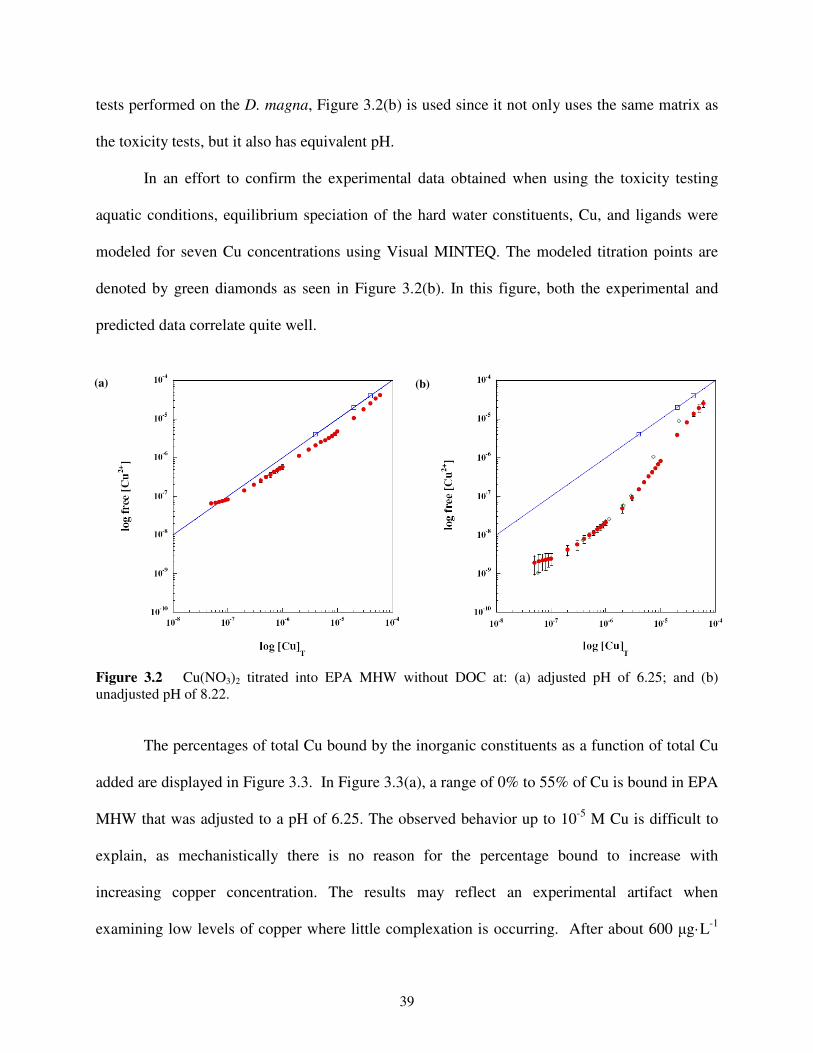
39
tests performed on the D. magna, Figure 3.2(b) is used since it not only uses the same matrix as
the toxicity tests, but it also has equivalent pH.
In an effort to confirm the experimental data obtained when using the toxicity testing
aquatic conditions, equilibrium speciation of the hard water constituents, Cu, and ligands were
modeled for seven Cu concentrations using Visual MINTEQ. The modeled titration points are
denoted by green diamonds as seen in Figure 3.2(b). In this figure, both the experimental and
predicted data correlate quite well.
Figure 3.2 Cu(NO3)2 titrated into EPA MHW without DOC at: (a) adjusted pH of 6.25; and (b)
unadjusted pH of 8.22.
The percentages of total Cu bound by the inorganic constituents as a function of total Cu
added are displayed in Figure 3.3. In Figure 3.3(a), a range of 0% to 55% of Cu is bound in EPA
MHW that was adjusted to a pH of 6.25. The observed behavior up to 10-5
M Cu is difficult to
explain, as mechanistically there is no reason for the percentage bound to increase with
increasing copper concentration. The results may reflect an experimental artifact when
examining low levels of copper where little complexation is occurring. After about 600 µg·L-1
(a) (b)

40
of Cu is added into the system, oversaturation occurs as the Cu concentration is much higher
than the carbonates in the water. Especially at a lower pH, metal binding is less prominent since
the dissolution of carbonic acid (H2CO3*) and bicarbonate (HCO3
-) are more prominent than
carbonate (CO32-
) yielding a lower carbonate Alk, thus leading to less overall metal
complexation.
Figure 3.3 Percent bound Cu in EPA MHW without DOC at: (a) adjusted pH of 6.25; and (b)
unadjusted pH of 8.22.
Figure 3.3(b) has all the same conditions as Figure 3.3(a) except the pH of the EPA
MHW is unadjusted and has a natural pH value of 8.22, resulting in the sample having a higher
carbonate Alk. With more Alk present, a larger amount of Cu is bound. The system is able to
bind an average of 97% of the Cu until nearly 1 mg·L-1
of Cu is added.
3.4.2 Cu Titration of EPA MHW with DOC
The concentration of free Cu2+
as a function of CuT in a system containing 6 ppm (3
mg·L-1
DOC) is shown in Figure 3.4. Again, the blue straight line denotes the Nernstian slope
(a) (b)

41
where unbound, free Cu2+
exists and the red dots represent the experimental data given from the
Cu2+
-ISE. Organic complexation has major binding pH values between 3.0 and 5.5, which
correlate to the dissociation values of carboxylic acid, the major binding constituent of fulvic
acid. Therefore, by adjusting the pH to 6.25, most of the binding can be attributed to organic
complexation and is exhibited in Figure 3.4(a). Other titrations were performed in a solution with
an unadjusted pH of 8.05 as seen in Figure 3.4(b).
Figure 3.4 Cu(NO3)2 titrated into EPA MHW with 6 ppm SRFA (3 mg·L-1 DOC) at: (a) adjusted pH of
6.25; and (b) unadjusted pH of 8.05.
The experimental data was also compared to a modeled titration in Visual MINTEQ.
These modeled results are denoted by green diamonds as seen in Figure 3.4(b). In this figure, the
experimental and predicted data deviate when low Cu concentrations are present. This is likely
due to the model not having the ability to accurately predict the strength of all of the DOC
binding sites. A thorough description of this topic can be found in Section 3.5: Synthesis of
Modeled Data.
(a) (b)

42
Figure 3.5 Percent bound Cu in EPA MHW with 6 ppm SRFA (3 mg·L-1 DOC) at: (a) adjusted pH of
6.25; and (b) unadjusted pH of 8.05.
The percentages of total Cu bound by fulvic acid and inorganic constituents are displayed
in Figure 3.5. A range of 15% to 88% of Cu is bound when the solution was adjusted to a pH of
6.25 shown in Figure 3.5(a). Maximum Cu binding is observed when 25 µg·L-1
is added into the
system. The presence of fulvic acid drastically increases the amount of Cu bound, which is
evident when comparing Figures 3.3(a) and 3.5(a). Even at low pHs, which favors free cupric
ions, there are still significant Cu complexes forming. In Figure 3.5(b), the same conditions exist
as in Figure 3.5(a), with the only difference being that the natural pH of the SRFA solution was
retained at a value of 8.05. Because more carbonate Alk is present than at a pH of 6.25, a much
larger amount of Cu is bound across a wide concentration range. An average of 99% of the Cu
remained bound until a total of 1 ppm of Cu was titrated.
The effects of Cu being titrated into EPA MHW with and without the presence of 6 ppm
SRFA (3 mg·L-1
DOC) at the pH of the natural water is combined and shown in Figure 3.6. Free
Cu2+
concentration is plotted as a function of CuT in the system as well as their modeled titration
(a) (b)

43
curves. Again, the blue straight line denotes the Nernstian slope where unbound, free Cu2+
exists.
The top red line represents the experimental data given from the Cu2+
-electrode when Cu(NO3)2
is only titrated into EPA MHW with its respective modeled data being represented by the solid
light green diamonds as shown in Figure 3.6(a). The bottom brown line represents the
experimental data from the Cu(NO3)2 being titrated into EPA MHW containing 6 ppm SRFA (3
mg·L-1
DOC) with its associated modeled data shown as the dark green diamonds seen in Figure
3.6(b).
Figure 3.6 Cu(NO3)2 titrated into EPA MHW: (a) without any SRFA at an unadjusted pH of 8.22; and
(b) with 6 ppm (3 mg·L-1 DOC) SRFA at an unadjusted pH of 8.05.
By way of directly comparing the effects of Cu binding to inorganic complexes in the
EPA MHW and Cu binding with DOC to form mostly organic complexes, the binding strength
of SRFA to form Cu-FA complexes over Cu-inorganic complexes can be observed in Figure 3.6.
Comparing single points in both of the titration curves can attest to the significant binding
capacity FA moieties possess. When 1·10-6
M (63.5 µg·L-1
) of Cu(NO3)2 is input to the system
where SRFA is not present, 97.6% of Cu is bound, whereas with SRFA present, 99.4% of Cu is
(a)
(b)

44
bound. The binding effects of Cu and SRFA are even more apparent at higher titration points.
When 1·10-5
M (635 µg·L-1
) of Cu(NO3)2 is titrated, 91.7% of Cu is bound in the system
containing only EPA MHW, while the system with SRFA still binds 96.9% of the Cu.
Figure 3.6 suggests that Visual MINTEQ can better predict the freed Cu2+
when
competition is limited to inorganic constituents of MHW than when organic molecules are also
introduced. In fact the experimental data in Figure 3.6(a) only deviates from the modeled data by
~6%. On the other hand, there is much more variation seen in Figure 3.6(b). At low
concentrations, the model predicts the first titration point to be ~60,000% lower than what was
found experimentally. However, at higher concentrations, deviation is ~5% different between
experimental and modeled values.
The discrepancy in the data could be attributed to instrumental error or inaccuracies in
Visual MINTEQ itself. One explanation is that a low-level measurement of the sample could not
be achieved since the concentration is below the sensing capabilities of the Cu2+
-ISE. Another
rationalization could be that the model does not have the power to predict the proper partitioning
of the SRFA and may be predicting too much or too little charge to accurately describe binding
site availabilities.
3.4.3 Zn Titration of Cu and EPA MHW with DOC
Although the Orion manual, as well as literature, explains that Zn ions will not be sensed
by the Cu2+
-ISE, a Zn titration into a solution of 6 ppm (3 mg·L-1
DOC) prepared in EPA MHW
was still performed.[57] The results of the titration can be seen in Figure 3.7. When Zn is added,
the electrode does sense ions in solution but this is attributed to the inert background electrolyte.

45
There is not an increase shown with each aliquot of Zn being added into solution demonstrating
that the Cu2+
-ISE does not sense Zn2+
.
Figure 3.7 Zn(NO3)2 titrated into EPA MHW with 6 ppm SRFA (3 mg·L-1 DOC) at an unadjusted pH of
7.97.
Titrations were performed in an effort to understand the competitive effects of Cu and Zn
for binding to DOC sites. A plot of the free Cu2+
concentration extrapolated from the Cu2+
-
electrode as a function of total zinc (ZnT) placed into either a 2·10-6
M or 2·10-5
M Cu(NO3)2
solution containing 6 ppm (3 mg·L-1
DOC) prepared in EPA MHW is shown in Figure 3.8. The
Cu was allowed to equilibrate in solution for 24 hours prior to titrating in Zn to assure Cu
binding to sites on the DOC of the SRFA was near equilibrium. If displacement of Cu by Zn is
occurring for binding sites then more free Cu will be detected in solution. The blue straight line
denotes the total Cu concentration placed into solution, the experimental data for free Cu are the
red dots, and the modeled data from Visual MINTEQ are the green diamonds.
Zn(NO3)2 titrations performed using a constant 2·10-6
M Cu(NO3)2, or 127 µg·L-1
Cu,
background are shown in Figure 3.8(a). The more Zn that is added, the more free Cu that is
detected. Even though the freed Cu2+
is nearly insubstantial compared to the CuT of the system,

46
this small increase of a toxic metal ion could greatly affect an aquatic organism such as D.
magna, which are susceptible to minute variations in trace metals. Figure 3.8(a) seems to agree
with the initial hypothesis of this work that Zn is displacing Cu. However, it cannot be
experimentally confirmed by the electrode method whether Zn is outcompeting Cu for binding
sites on the DOC or the inorganic ligands. It is possible, though, to compare the results to the
modeled species distribution to confirm competition is occurring at DOC binding sites. The
increase in Cu2+
as more Zn is titrated is also demonstrated with the modeled points, denoted as
green diamonds, further confirming the hypothesis.
Figure 3.8 Zn(NO3)2 titrated into EPA MHW with 6 ppm SRFA (3 mg·L-1 DOC) at: (a) 2·10
-6 M
Cu(NO3)2 present, pH of 7.80; and (b) 2·10-5
M Cu(NO3)2 present, pH of 7.75.
One possible explanation for the model predicting more free Cu2+
in Figure 3.8 than what
the experimental data suggests is that the binding constant of Zn (KaZn) within the program could
be too strong, making it more difficult for Cu to be bound to DOC. Another explanation involves
the kinetics of the Cu2+
binding to the SRFA. Cu(NO3)2 was equilibrated in the EPA MHW
containing SRFA for at least 24 hours prior to titrating in Zn(NO3)2. Therefore, Cu2+
would bind
(a) (b)

47
at a fairly fast rate at the strong sites (carboxylic groups) since the pH of the water is
approximately 8, much higher than the pKa of the carboxylic groups. Conversely, a much slower
binding rate is occurring at the weak sites (phenolic groups) since the solution is below the pKa
of the weak sites. However, since the Cu(NO3)2 was equilibrated for 24 hours, some of these
weaker sites are able to complex. Even though weak sites are not as capable of binding, they
often have high site density in fulvic acid, thus have the ability to take a large role in binding.
Since the experimental Cu2+
had time to fill both the strong and some weak sites of the SRFA
solution, more of the Cu2+
will be bound compared to the modeled results which assumes a rapid
titration. This most likely explains the discrepancy between experimental and modeled results.
Figure 3.9 Percent bound Cu in EPA MHW with 6 ppm SRFA (3 mg·L-1 DOC) when Zn(NO3)2 is
titrated into solution with: (a) 2·10-6
M Cu(NO3)2 present, pH of 7.80; and (b) 2·10-5
M Cu(NO3)2 present,
pH of 7.75.
Figure 3.9 displays the percentages of total Cu bound by fulvic acid and inorganic
constituents as a function of total Zn added. In this figure, it is important to note that the y-axis
has a truncated range from previous graphs with only displaying 99% to 100% Cu bound. The
percent Cu bound when the concentration is constant at 2·10-6
M Cu(NO3)2 and Zn is being
(a) (b)
48
titrated into the SRFA solution is shown in Figure 3.9(a). Here, the average percent bound Cu for
the entire titration is 99.8%. After approximately 1·10-5
M (~650 µg·L-1
) of Zn has been titrated
into solution, free Cu2+
appears to begin an exponential increase, but in fact is increasing at a
very slow rate. In fact, after 1.5·10-4
M (~10 mg·L-1
) of Zn has been titrated, 99.5% of Cu is still
bound in solution.
The results of having a whole order of magnitude higher in Cu concentration of 2·10-5
M
Cu(NO3)2 present while Zn is titrated into a SRFA solution can be seen in Figure 3.9(b). Having
a higher background Cu concentration caused slightly less overall Cu to be freed during the
titration as 0.3% more was bound in the 2·10-5
M Cu(NO3)2 than in the 2·10-6
M Cu(NO3)2
solution after 10 mg·L-1
Zn had been titrated. Interestingly, both the solution with 2·10-5
M
Cu(NO3)2 and the solution containing 2·10-6
M Cu(NO3)2 demonstrated similar trends in their
curves with the biggest resemblance being that Cu complexes start to break down after 1·10-5
M
(~650 µg·L-1
) Zn has been titrated into solution.
3.4.4 Cu and Zn in SRFA Solution after 24-hour Equilibration
Pre-titrated samples of various concentrations ranging from 5·10-8
M to 1.3·10-4
M of
Zn(NO3)2 (~3 µg·L-1
to ~9 mg·L-1
Zn) were placed into a solution containing 2·10-6
M Cu(NO3)2
and 6 ppm (3 mg·L-1
DOC) prepared in EPA MHW. Similar to the other Cu and Zn titrations, the
effect of free Cu2+
concentration as a function of ZnT placed into the solution was plotted and is
shown as the green dots in the (b) line in Figure 3.10. These samples allowed for both Cu and Zn
to equilibrate in solution for 24 hours to take a more realistic approach.
Figure 3.10 combines data from the 24-hour titration and Figure 3.8(a) to show the
differences in the free Cu2+
concentration extrapolated from the Cu2+
-electrode as a function of

49
total zinc (ZnT). The red dots denote are data from Figure 3.8(a) where Cu(NO3)2 was
equilibrated for 24 hours in EPA MHW with 6 ppm (3 mg·L-1
DOC) SRFA. The green diamonds
represent data from Cu(NO3)2 equilibrating with EPA MHW containing 6 ppm (3 mg·L-1
DOC)
SRFA for 24 hours and then another equilibration after Zn was added.
Figure 3.10 Zn(NO3)2 titrated into EPA MHW with 6 ppm SRFA (3 mg·L-1 DOC) with a pH of 7.80:
(a) rapid titration of 2·10-6
M Cu(NO3)2 present; and (b) 24-hour equilibration of 2·10-6
M Cu(NO3)2
present.
Figure 3.10 exemplifies the fact that rapid titrations versus equilibrated samples yield
much different results. When Cu is added to solution, there is immediate binding of the metal
and the strong groups (carboxylic acid) on the SRFA. This is clearly demonstrated in Figure
3.4(b) where Cu2+
is shown to bind to the SRFA but not as strongly as when Cu is allowed to
equilibrate for 24 hours in EPA MHW containing SRFA as was shown in Figure 3.8(a).
However, when allowed to equilibrate for extended periods (≥24 hours) the weaker sites
(phenolic groups) of the SRFA begin to demonstrate that they play a key role in the chelation of
Cu2+
. Figure 3.10 demonstrates the role of strong and weak binding sites as the Cu(NO3)2 was
allowed to equilibrate for at least 24 hours prior to adding Zn(NO3)2 which was then equilibrated
(a)
(b)

50
again for 24 hours. The amount of free Cu2+
is almost a whole order of magnitude lower than the
rapid titration.
Although rapid titrations are more practical since aliquots of solution can be added and
monitored sequentially with little H2CO3* affecting the sample, it appears that the 24-hour
samples lend a more realistic interpretation of the free metal available. About a 45% difference
in Cu2+
exists between the two titration approaches. Such a difference in Cu2+
could definitely
have a critical effect on D. magna. However, although the actual data points differ spatially,
they have nearly identical Cu binding percentages. In fact, the difference of bound Cu between
the two data sets averages to 0.12%. The two curves in Figure 3.10 also share similarities in that
Cu is freed as more Zn is added, which agrees with the hypothesis.
3.5 Synthesis of Modeled Data
While Visual MINTEQ is capable of simulating a titration, this method was not
employed as the pH of the experimental titration varied slightly with each addition of metal.
Therefore, eight points were chosen from the experimental data and input into the model with
each point’s correlating pH, temperature and Alk.
3.5.1 Explanation of Variability between Modeled and Experimental Data Regarding
DOC
The data presented here reflects that of the experimental data as well as the computational
values gained from modeling the experimental conditions in Visual MINTEQ. There was
generally good agreement between the experimental and modeled points for all of the titrations.
However, in some cases, the experimental and modeled points varied from each other at lower

51
pH values when they contained humic substances. This is likely due to the fact that the DOC
used in the model is based on the SHM.
In the SHM, a discrete-site approach is taken to illustrate the dependence of the
dissociation of the humic substance as a function of pH. These discrete sites have differing acid
strengths and therefore will have differing intrinsic dissociation constants. For the SHM, eight
sites are assigned to each humic molecule whereby four sites are strong acid sites and are used to
describe the carboxylic acid groups in the molecule, and the other four sites are weak acid sites
which are attributed mostly to the phenolic groups in the molecule.[21] The SHM uses seven
adjustable parameters that are inputs for the SHM to describe the proton dissociation reaction
that is occurring. The parameters are generic values taken from an average of various humic
substances.[37] The variability between humic substances from different regions and
environments could have different metal binding characteristics thus explaining why modeled
data points and experimental data points differ. Furthermore, generic values of fulvic acid in the
SHM (as well as other geochemical models like NICA-Donnan) have been shown to, at times,
not satisfactorily illustrate Cu2+
activity for samples.[58]
3.6 Conclusions
A Cu2+
-ISE was used to determine the amount of free Cu2+
that is displaced as more
Zn(NO3)2 was titrated into a solution of 6 ppm (3 mg·L-1
DOC) SRFA prepared in EPA MHW
with a 2·10-6
or 2·10-5
M Cu(NO3)2 concentration. The experimental titrations were compared
with modeled titrations performed in Visual MINTEQ. In cases where titrations were done into
EPA MHW without any SRFA present, the experimental data was nearly identical to the
modeled data. However, the addition of DOC caused experimental data to deviate from the
modeled titration. This is likely due to the model not having the ability to accurately predict all

52
of the dissociation constants associated with SRFA, making binding sites appear to become more
or less available to form complexes with metal ions.
By observing the increase in Cu2+
, an estimate of the bioavailability of this ion can be
made and related to the toxicity tests of the D. magna. Experimental titrations demonstrated that
as more Zn is being added into the system, there, consequently, is more Cu2+
that is becoming
unbound denoted by its increase in all of the titrations. This not only agrees with the modeled
data in Chapter 2, it also supports the toxicity results and, correspondingly, the hypothesis that
Zn displaces Cu which would indeed cause more Cu2+
to be bioavailable and be more toxic to D.
magna among other aquatic organisms.

53
CHAPTER 4
FLOW FIELD-FLOW FRACTIONATION WITH INDUCTIVELY COUPLED
PLASMA-MASS SPECTROMETRY DETECTION
4.1 Introduction
Field-flow fractionation (FFF) was engineered and patented by J. Calvin Giddings in
1966.[59] FFF is a separation technique to which a force field is applied perpendicular to a flow
stream in a narrow channel.[59],[60]. A variety of gradients can be applied but commercially
available ones include: thermal (thermal FFF), centrifugal (sedimentation FFF), electrical fields
(electrical FFF), magnetic (magnetic FFF), or flow field (Fl FFF).[61]-[63] Fl FFF was the sub-
technique utilized for this work because of its ability to separate and characterize natural colloids
(up to 1 µm) and nanoparticles (1-100 nm). Additionally, Fl FFF is the most universally and
most frequently used of all the sub-techniques since it lends rapid analyses, is absent of shear
forces, has adjustable separation parameters, and can be interfaced with other analytical
techniques.[60],[63]
Although Giddings successfully demonstrated the separation versatility of FFF through a
variety of samples ranging from polystyrene particles to proteins, the technique was not widely
used until it was hyphenated with other techniques in the late 1980’s and early 1990’s. Coupling
instruments allow for better detection and a wider versatility of samples. Specifically, the hy-
phenation of FFF with inductively coupled plasma-mass spectrometry (ICP-MS) is beneficial
when analyzing metal-containing environmental samples because the particles in the sample are
not only size-fractionated, but are also quantified in the ppt range.[64]

54
Beckett and co-workers were the first to suggest hyphenating FFF and ICP-MS in
1991.[65],[66] One year later, Beckett published his work with FFF and ICP-MS, although at
this time the samples were run off-line which required flash freezing all of the samples and
digesting with nitric acid (HNO3) then running the sample in an ICP-MS.[66],[67] In 1992,
Taylor and co-workers reported the first on-line coupling of Fl FFF with ICP-MS and determined
the particle size and elemental distribution of trace metals in environmental water samples.[68]
Since the initial introduction of online Fl FFF-ICP-MS, multiple fields have utilized the powerful
technique varying from food sciences to pharmaceuticals. However, the environmental sciences
are currently the most dominant in the Fl FFF-ICP-MS realm.
Fl FFF-ICP-MS has not yet been used as an analytical tool for determining the binding of
Cu or Zn to SRFA in an effort to understand the bioavailability of these metals. In order to try to
further explain the analytical results found using the Cu2+
-ISE in Chapter 3 regarding the appar-
ent increase in Cu2+
as more Zn is placed into solution with and without DOC, Fl FFF-ICP-MS
was employed. The work presented in this chapter takes a qualitative approach concerning multi-
metal competition of trace metals in natural waters. A total understanding of the competitive
interactions of Cu2+
and Zn2+
is not demonstrated. Instead, the practicability of Fl FFF-ICP-MS
as a powerful separation technique as well as a metal quantifier is investigated in this proof of
concept study.
4.2 Fl FFF Theory
Fl FFF, as shown in Figure 4.1, employs a hydrodynamic field that is comprised of a
cross flow running perpendicular to the channel flow. Fractionation of the sample occurs in a
thin channel that is composed of one block (if asymmetrical FFF) or two blocks (if symmetrical
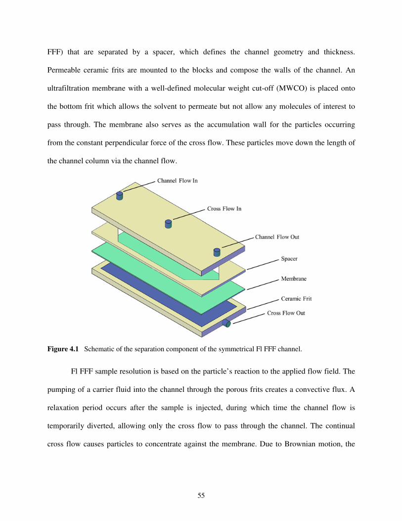
55
FFF) that are separated by a spacer, which defines the channel geometry and thickness.
Permeable ceramic frits are mounted to the blocks and compose the walls of the channel. An
ultrafiltration membrane with a well-defined molecular weight cut-off (MWCO) is placed onto
the bottom frit which allows the solvent to permeate but not allow any molecules of interest to
pass through. The membrane also serves as the accumulation wall for the particles occurring
from the constant perpendicular force of the cross flow. These particles move down the length of
the channel column via the channel flow.
Figure 4.1 Schematic of the separation component of the symmetrical Fl FFF channel.
Fl FFF sample resolution is based on the particle’s reaction to the applied flow field. The
pumping of a carrier fluid into the channel through the porous frits creates a convective flux. A
relaxation period occurs after the sample is injected, during which time the channel flow is
temporarily diverted, allowing only the cross flow to pass through the channel. The continual
cross flow causes particles to concentrate against the membrane. Due to Brownian motion, the

56
particles diffuse against the cross flow. Because each particle size has its own unique diffusion
coefficient, a positional equilibrium is achieved by the balancing of the diffusive flux.
Particles sharing the same diffusion coefficient move through the channel in an
equilibrium cloud that has a thickness () that is affected by both the cross flow velocity (G) and
the diffusion coefficient of the particles (H).[64] and H are directly proportional whereas and
G are inversely proportional. Therefore, when H is a small value and/or if G is a large value,
will be smaller which correlates to the sample having a longer retention time in the channel.[69]
This relationship is shown in Equation 4.1.
=I
J
(4.1)
After relaxation, the channel flow is redirected back through the channel and a laminar
flow is achieved. Laminar flow allows for orderly displacement of particles parallel to the
channel.[70] However, the particles do not all move at the same rate due to a parabolic distri-
bution of flow velocities across the channel, causing a higher flow profile in the middle of the
channel and a lower flow profile towards the walls of the channel where there is more friction.
Thus, the smaller particles tend to reach an equilibrium position faster than larger particles since
they have higher diffusion rates and, subsequently, the smaller particles will elute first while the
larger particles elute last.
In some cases there are sample constituents that remain unrelaxed throughout the entire
run and will reach the detector before even the smallest particle does appearing as a response.
These particles form a so-called “void” peak, but are not considered in data calculations. The
relationship between the retention time (KE) of the sample, the channel thickness (L), and cross
flow force (@) are relatable through Equations 4.2 and 4.3, where K7 is the void volume, M is
Boltzmann’s constant, and > is the absolute temperature.

57
DN
DO=
P
%=
|;|P
R:
(4.2)
@ = S|G| = M>|J|
I= 3TU|G|V (4.3)
The retention time in the channel is proportional to the channel flow rate, the channel thickness,
the viscosity of the carrier fluid (U), the cross flow velocity, and the hydrodynamic diameter of
the particle (V). Equations 4.2 and 4.3 describe how the sample’s retention time correlates to the
sizing of the particles in the sample. Since the void time is the length of time it takes to get one
full channel volume through the column, the sample elution time can be calculated and directly
correlated to particle size. Simply, the retention time of a particle is related to the channel flow
rate. In this way, fractograms of intensity as a function diameter can be graphed for easy
analysis.
4.3 Experimental
Prior to use, all sample containers were acid-washed for at least 24 hours then rinsed
copiously with deionized water with a resistivity of 18.2 MΩ cm (Barnstead NANOpure
ultrapure water system). All storage containers were polyethylene or Teflon®
to eliminate any
unwarranted metal leaching. The chemicals used were reagent grade (98%) or better Fisher
Scientific products. ICP-MS stock Cu and Zn metals stabilized in HNO3 (High Purity Standards,
Charleston, South Carolina, USA) were used in all of the samples. The humic substance used
was SRFA (Standard II, IHSS, St. Paul, Minnesota).
4.3.1 Sample Preparation
Vials containing Cu, Zn, or both were prepared so that final concentration of Cu was
1.57·10-6
M (100 µg·L-1
) and final concentrations of Zn were 1.53·10-4
M (10 mg·L-1
). A sub-

58
sample was taken of each stock solution for analysis on an ICP-AES for confirmation of the
metal concentrations.
All samples were prepared in 18.2 MΩ UV-treated water (Barnstead NANOpure ultra-
pure water system) containing either 20 ppm (10 mg·L-1
DOC) or 60 ppm (30 mg·L-1
DOC) of
SRFA. Samples were then equilibrated for at least 24 hours to ensure metal binding to sites on
the DOC. The concentrations were calculated by mass and confirmed by a total organic carbon
(TOC) Shimadzu TOC 1000 Carbon Analyzer (Shimadzu, Columbia, MD, USA). These solu-
tions were stored in polyethylene or Teflon®
containers and were placed in a 4°C refrigerator
when not in use to limit any degradation that could occur.
The Fl FFF carrier fluid was composed of 4 mM sodium chloride (NaCl, analytical grade,
Fisher Scientific) and 0.1 mM sodium azide (NaN3, a microbiocide, analytical grade, various
sources). Generally, higher ionic strength lends to better peak resolution but poorer overall
sample recovery. Although 4 mM NaCl is considered moderate ionic strength, several other
groups have run samples in a much higher ionic strength (10 mM NaCl) and had recoveries that
were acceptable.[71]
4.4 Fl FFF-ICP-MS Instrumentation
The Fl FFF model used for analysis was an F-1000 fractionation channel (formerly
FFFractionation, Salt Lake City, Utah, USA; now Postnova Analytics, Salt Lake City, Utah,
USA and Landsberg, Germany). The sample was introduced into the fractionator via a stainless
steel Rheodyne 50 µL injection loop. A silicone-coated regenerated cellulose membrane with a
molar mass cut-off of 1 kDa (Postnova Analytics, Salt Lake City, Utah, USA) was placed upon
the spacer with a thickness of 254 µm. Two Accu-flow Series II high performance liquid

59
chromatography (HPLC) pumps (Fisher Scientific, Pittsburg, Pennsylvania, USA) were used to
move the carrier fluid through the channel and cross flows.
An online ISCO Model 229 ultraviolet/visible (UV/Vis) absorbance detector (Teledyne
ISCO, Inc., Lincoln, Nebraska, USA) with a 254 nm filter was used to characterize the sample
and to detect the polystyrene sulfonate (PSS) size standards (American Polymer Standards
Corporation, Mentor, Ohio, USA). UV254 is used as it is near the absorbance band for both the
PSSs and fulvic acid. This wavelength is frequently used in analyses of aquatic environmental
samples since this is the intense emission line for spectrometers with mercury-vapor lamps.[72]
A Truflow flow monitor (0-4 mL range, Glass Expansion, West Melbourne, Australia) was used
to gauge the flow rate of the sample and was located downstream of the UV/Vis detector but
upstream of the ICP-MS. UV/Vis data acquisition was obtained through the FFFractionation
software FLOW (version 2.0.0 alpha 3).
4.4.1 Fl FFF Instrumental Operations
The full operation of Fl FFF is detailed in this section. First, an injection-relaxation
occurs whereby fresh carrier liquid composed of sodium chloride (NaCl, analytical grade, Fisher
Scientific) and sodium azide (NaN3, a microbiocide, analytical grade, various sources) is
delivered via one of the HPLC pumps (pump 1). Pump 1 transports the carrier fluid at a rate of
1.0 mL·min.-1
to the inlet of the channel and served as the channel flow. Concurrently, the carrier
fluid was also delivered at a rate of 3.0 mL·min.-1
by the other HPLC pump (pump 2), which
served as the cross flow. A relaxation period of 2 minutes occurred following sample injection.
Relaxation enables the sample components to achieve an equilibrium position before the run
begins. Following relaxation, the six-port switching valve opens the main flow outlet allowing

60
for the channel flow to push the particles through the system. Specific analytical parameters for
separation of the sample using the Fl FFF are shown in Table 4.1.
Table 4.1 Fl FFF instrumentation parameters used for separation and characterization of Cu- and Zn-FA
complexes.
Parameter Description
Fl FFF Postnova F-1000 symmetrical
Injection Volume 50 µL loop
Membrane 1 kDa regenerated cellulose
Carrier Fluid 4mM NaCl, 0.1mM NaN3
Channel Flow 1.0 mL·min.-1
Cross Flow 3.0 mL·min.-1
Relaxation Time 2.0 min.
Fractogram Time 12 min.
Absorbance λ 254 nm
UV Detector ISCO 229
4.4.2 Fl FFF Hyphenation with ICP-MS
The Fl FFF was interfaced to a PerkinElmer NexION 300Q ICP-MS (PerkinElmer,
Waltham, Massachusetts, USA) and the PerkinElmer software (version 1.3) was used for
elemental analysis. The Cu isotopes monitored were 63
Cu and 65
Cu and the Zn isotopes
monitored were 66
Zn and 68
Zn. The integration dwell time was 250 ms, resulting in
approximately one data point being collected each second.
Table 4.2 ICP-MS instrumentation parameters used for separation and characterization of Cu- and Zn-
FA complexes by Fl FFF-ICP-MS.
Parameter Description
ICP-MS PerkinElmer NexION 300Q
Masses Monitored 63
Cu, 65
Cu, 66
Zn, 68
Zn
Dwell time per AMU 250 ms
All samples were run online, which allows for the isotope intensities to be monitored as
the fractionated sample elutes from the Fl FFF in real time. An 115
In internal standard was chosen
61
as it is monoisotopic and did not interfere with the isotopes being analyzed. An internal standard
was used to monitor if instrumental drift occurred. Because no significant instrument drift was
detected, the analyte concentrations remained absolute without any normalization. Specific ana-
lytical parameters for characterization of the sample using ICP-MS are shown in Table 4.2.
4.5 Calibration
Molecular weight and concentration calibrations for the Fl FFF and concentration
calibrations for the ICP-MS should be done if analyzing the data quantitatively. There are
multiple calibration approaches that are considered acceptable when analyzing fractograms. For
ICP-MS fractograms, one of the most common and versatile methods for converting metal
intensity to a concentration is to inject various metals with known masses and create a calibration
curve by correlating their peak area to a concentration. Similarly, a molecular weight calibration
can be performed by correlating the peak maximum elution time to known molecular weight
standards’ elution times.[73]
However, with regards to this project, only a qualitative approach was taken, thus exact
concentrations were not determined. Nevertheless, a calibration for Fl FFF using PSS standards
(American Polymer Standards Corporation, Mentor, Ohio, USA) was performed. The PSSs were
used for obtaining the molecular weight of the samples. By way of injecting a known PSS
molecular weight sample into the fractionator, the particle molecular weight as a function of its
elution time can be plotted. So long as the operating conditions of the fractionator are identical
for the calibration and for the experimental data, the metal-fulvic acid complexes can be
characterized via UV absorption.

62
Prior to sampling, the Fl FFF was calibrated using at least three PSSs. These PSS samples
had seven different standard sizes of 1.43, 3.42, 4.80, 6.50, 10.43, 15.45, 20.00, and 31.00 kDa
and each were made to have a final concentration of approximately 30 mg·L-1
. A typical FFF-
UV fractogram is displayed in Figure 4.2 whereby three molecular weights (1.43, 6.50, and
15.45 kDa) are depicted. By way of extrapolating the maximum UV absorbance of each standard
particle and correlating that to an elution time, a calibration plot of these standard sizes can be
created and is shown in the inset of Figure 4.2. For most of the calibrations, the linearity of the
slope was found to be 0.995±0.005.
Figure 4.2 FFF-UV Fractogram for calibration using 1.43, 6.50 and 15.45 kDa PSS standards where
UV λ = 254 nm, channel flow = 1.0 mL·min.-1
., cross flow = 3.0 mL·min.-1
. Inset: Experimental linear
regression curve for sizing where Fl FFF-UV absorbance at peak maximum is plotted as a function of
time.
4.6 Sample Recovery
Since the interest was to qualitatively analyze the fractograms, sample recoveries were
not taken into account. However, studies have shown that sample recovery is rarely 100% of the

63
injected sample, often ranging between 85% to 99%.[72],[74] The phenomenon is often
attributed to the adhesion of the sample to the membrane.[69],[74] The use of a regenerated
cellulose membrane instead of a polyether sulfone membrane can increase recovery, especially
with environmental samples which often contain humic substances.[75] Furthermore, it is
speculated that samples adjusted to a higher pH have a higher recovery than those at more acidic
pHs.[76] For the sake of maintaining the integrity of a given environmental sample, however, it
would not be more important to have a higher recovery over characterizing the sample under
relevant conditions.
4.7 Results & Discussion
A proof of concept study utilizing Fl FFF-ICP-MS to qualitatively determine the
competitive interactions of Cu and Zn for binding to sites on the SRFA complex was performed.
Results from the toxicity tests with the D. magna indicated that the LD50 of Cu was
approximately 100 µg·L-1
. Based on these results, the Cu concentration chosen for all of the
samples was 100 µg·L-1
whereas the Zn concentration was either 0 µg·L-1
or 10 mg·L-1
. If Zn
were displacing Cu from the SRFA, it would be more evident at a higher concentration of 10
mg·L-1
than at one that was closer or matched the Cu concentration. However, the matrix used
for these samples was not EPA MHW, but rather 18.2 MΩ UV-treated water (Barnstead
NANOpure ultrapure water system). This was to focus on the interactions of Cu and Zn with the
fulvic acid in order to efficiently develop an analytical procedure. The NANOpure water re-
mained unbuffered at a pH of 5.9 so that organic complexes that formed would not be competing
with any inorganic complexes. However, the pH decreased to 4.5 with the addition of the 20 ppm
SRFA. The effect of adding Cu or Zn, however, did not change the pH of the 20 ppm SRFA in

64
NANOpure water and remained at 4.5. The SRFA concentration was increased to 20 ppm,
therefore also increasing the DOC concentration to 10 mg·L-1
. The increase of the SRFA
concentration was so that the Cu- and Zn-organic complexes could be detectable in the
fractograms. The qualitative results using Fl FFF-ICP-MS provides limited agreement with the
hypothesis, yet the practicability of this analytical technique is demonstrated.
4.7.1 Identification of SRFA using Fl FFF-ICP-MS
Initially, a ten-fold increase of the SRFA concentration utilized in the toxicity tests was
used for preparing samples. However, 60 ppm SRFA (30 mg·L-1
DOC) overloaded the UV
detector and required a lower sensitivity to be used. Instead of reducing the detector sensitivity,
the SRFA solution was reduced to 20 ppm SRFA (10 mg·L-1
DOC). Figure 4.3(a) displays the 60
ppm SRFA Fl FFF-UV fractogram at the lower UV detector sensitivity whereby the relative
intensity is actually lower than the less concentrated 20 ppm SRFA fractogram shown in Figure
4.3(b).
Figure 4.3 Fl FFF-UV fractogram of: (a) 60 ppm SRFA (30 mg·L-1
DOC) at a lower UV sensitivity; and
(b) 20 ppm SRFA (10 mg·L-1
DOC) at a higher UV sensitivity.
(a) (b)
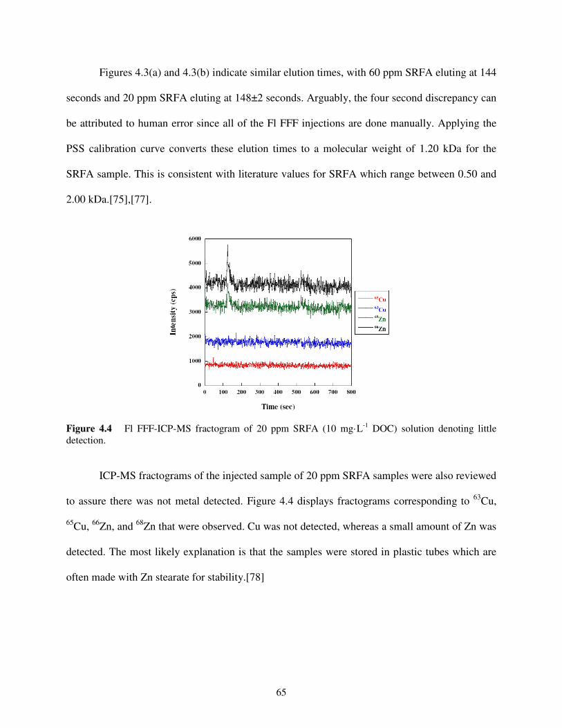
65
Figures 4.3(a) and 4.3(b) indicate similar elution times, with 60 ppm SRFA eluting at 144
seconds and 20 ppm SRFA eluting at 148±2 seconds. Arguably, the four second discrepancy can
be attributed to human error since all of the Fl FFF injections are done manually. Applying the
PSS calibration curve converts these elution times to a molecular weight of 1.20 kDa for the
SRFA sample. This is consistent with literature values for SRFA which range between 0.50 and
2.00 kDa.[75],[77].
Figure 4.4 Fl FFF-ICP-MS fractogram of 20 ppm SRFA (10 mg·L-1
DOC) solution denoting little
detection.
ICP-MS fractograms of the injected sample of 20 ppm SRFA samples were also reviewed
to assure there was not metal detected. Figure 4.4 displays fractograms corresponding to 63
Cu,
65Cu,
66Zn, and
68Zn that were observed. Cu was not detected, whereas a small amount of Zn was
detected. The most likely explanation is that the samples were stored in plastic tubes which are
often made with Zn stearate for stability.[78]

66
4.7.2 Data Analysis of Cu-FA and Zn-FA Complexes by Fl FFF-ICP-MS
A Cu-FA or Zn-FA complex could be given a relative concentration based on an ICP-MS
intensity calibration curve which exchanges the ordinate axis of the Fl FFF-UV fractogram from
intensity to concentration. However, since the focus of these experiments was to qualitatively
analyze the Cu-FA complexes, the actual concentration of Cu that is bound in a Cu-FA complex
was not determined. Instead, peak areas were summed using the trapezoidal rule and used to
compare the masses of the complexes. Baseline corrections of the Fl FFF-UV fractograms were
done using the FFFAnalysis software. Baseline corrections of the Fl FFF-ICP-MS fractograms,
however, were accomplished by subtracting out the value for the average of the last 180 data
points which are basically flat-lined and show little deviation from data point-to-data point.
Equation 4.4 describes the peak summation approach taken, where the mass (W) equals a
data point collected at a given time (K) and the time associated to the preceding collected point
(K&). The time element is multiplied by the Fl FFF channel flow rate (q) as well as the
concentration (+). The data points for summation are collected by the ICP-MS ().
W = (K − K&) ∗ Y ∗Z[\Z
(4.4)
By way of applying Equation 4.4 to every point gathered from the eluted ICP-MS peak,
the sum of all the points associated can give way to the Cu or Zn that is bound to the SRFA.
From a qualitative point of view, these masses can simply be summed and left as an arbitrary
value and not related to a specific concentration.
4.7.3 Identification of Cu-FA and Zn-FA Complexes by Fl FFF-ICP-MS
To understand the effects of Cu in relationship to the metal binding to SRFA or being
displaced by Zn, various samples were prepared for analysis by Fl FFF coupled to an ICP-MS. A

67
Cu concentration of 100 µg·L-1
was used in all of the samples while the Zn concentration varied
between 0 µg·L-1
and 10 mg·L-1
. The matrix used for these samples was deionized water with a
resistance of 18.2 MΩ cm (Barnstead NANOpure ultrapure water system) containing 20 ppm
SRFA (10 mg·L-1
DOC). All samples were left unbuffered which resulted in a pH of 4.5 whether
metals were present or not. Again, this was for the simplicity of viewing the competitive effects
of Cu and Zn with DOC sites without the added difficulty of analyzing hard water complexes.
Figure 4.5 is an Fl FFF-UV fractogram generated from the injection of a Cu sample with
a concentration of 100 µg·L-1
in a 20 ppm SRFA (10 mg·L-1
DOC) solution. The peak maximum
has an elution time of 146 seconds correlating to a molecular weight of approximately 1.1 kDa.
The UV data gathered from the Fl FFF affirmed the presence of a SRFA which is consistent with
the elution of 20 ppm SRFA shown in Figure 4.3(b) which had a molecular weight of 1.2 kDa.
Figure 4.5 Fl FFF-UV fractogram of 100 µL·L-1
Cu in a 20 ppm SRFA (10 mg·L-1
DOC) solution.
Once the UV data confirmed the presence of SRFA, the MS data from the ICP-MS was
used to identify if any Cu, Zn, or both metals were bound to the DOC. If bound, the metals
would be evident in the ICP-MS fractograms. If unbound, the metals should theoretically remain

68
in their ionic form and pass through the Fl FFF membrane since the MWCO was 1 kDa and Cu2+
and Zn2+
are much smaller than this cut-off.
The resulting FFF-ICP-MS fractogram for the injection of a 100 µg·L-1
Cu sample in a 20
ppm SRFA (10 mg·L-1
DOC) solution is shown in Figure 4.6. Peak area analyses were
performed of the fractogram using Equation 4.4 and the results are shown in Table 4.3. Area
summations yielded values of approximately 1300 arbitrary units (a.u.) of 65
Cu and 2800 a.u. of
63Cu. However, there were also 200 a.u. of
68Zn and 300 a.u. of
66Zn detected. Again, this is
most likely due to Zn being a plasticizing agent and could be leaching into the samples. The Zn
values shown in Table 4.3 were subtracted from subsequent samples containing Zn in order to
normalize the data. The strength in Fl FFF in generating highly reproducible fractograms is also
shown in Figure 4.6, where overlays of the fractograms are congruent.
Figure 4.6 Fl FFF-ICP-MS overlay fractograms of replicate runs of 100 µg·L-1
Cu in a 20 ppm SRFA
(10 mg·L-1
DOC) solution.
Table 4.3 Integration values of Fl FFF-ICP-MS fractogram of 100 µg·L-1
Cu in a 20 ppm SRFA (10
mg·L-1
DOC) solution.
65Cu (a.u.)
63Cu (a.u.)
68Zn (a.u.)
66Zn (a.u.)
1300±100 2800±250 200±50 300±50

69
A Fl FFF-UV fractogram of a Cu and Zn sample with a concentration of 100 µg·L-1
and
10 mg·L-1
, respectively, in a 20 ppm SRFA (10 mg·L-1
DOC) solution is shown in Figure 4.7. A
large Zn concentration was used to clearly see the effects Zn has on Cu complexes. As with the
other samples, the UV data affirmed the presence of SRFA and paralleled the other UV data
collected. The peak maximum had an elution time of 148 seconds correlating to a molecular
weight of approximately 1.2 kDa. Fl FFF-ICP-MS fractograms detected that both Cu and Zn
were bound to the DOC is shown below in Figure 4.8.
Figure 4.7 Fl FFF-UV fractogram of 100 µL·L-1
Cu and 10 mL·L-1
Zn in a 20 ppm SRFA (10 mg·L-1
DOC) solution.
Equation 4.4 was again applied to sum the fractogram peaks and the results are shown in
Table 4.4. Summation values did not demonstrate a significant decrease in Cu with Zn present in
a high concentration (10 mL·L-1
). There was again approximately 1300 arbitrary units (a.u.) of
65Cu detected which is equivalent to the sample containing only 100 µg·L
-1 Cu and 0 µg·L
-1 Zn.
Similarly, 63
Cu summations resulted in a value of 2750 a.u. which also correlates to a decrease in
~2% of 63
Cu with Zn present. The resultant Zn values from peak summation yielded 2700 a.u. of
68Zn and 4300 a.u. of
66Zn, which compare relatively well with their expected isotopic ratio. The

70
natural isotopic abundance for 68
Zn and 66
Zn are 18.8% and 27.9%, respectively. Data from the
fractograms estimates an isotopic abundance of 18.0% and 28.7% for 68
Zn and 66
Zn,
respectively.
Figure 4.8 Fl FFF-ICP-MS fractogram of 100 µg·L-1
Cu and 10 mg·L-1
Zn in a 20 ppm SRFA (10
mg·L-1
DOC) solution.
Table 4.4 Integration values of Fl FFF-ICP-MS fractogram of 100 µg·L-1
Cu and 10 mg·L-1
Zn in a 20
ppm SRFA (10 mg·L-1
DOC) solution.
Sample 65
Cu (a.u.) 63
Cu (a.u.) 68
Zn (a.u.) 66
Zn (a.u.)
100 µL·L-1
Cu 1300±100 2800±250 200±50 300±50
100 µL·L-1
Cu, 10 mL·L-1
Zn 1300±125 2750±300 2700±300 4300±450
To determine the amount of unbound metal that did not pass through the Fl FFF membrane
thus reaching the ICP-MS, a sample with a Cu concentration of 100 µg·L-1
in a 20 ppm SRFA
solution was injected followed by a field off injection of two Cu concentrations. The Cu
concentrations used were Cu-only samples of 10 µg·L-1
and 100 µg·L-1
. Figure 4.9 displays the
resulting Fl FFF-ICP-MS fractogram.
Specific to this project, the second field off Cu injection of 100 µg·L-1
shown is most
important as it is relatable to all of the other Cu samples which also had concentrations of 100

71
µg·L-1
. The peak area summations resulted in values of approximately 1400 a.u. of 63
Cu and
3000 a.u. of 65
Cu for the 100 µg·L-1
Cu-only injection. Overall, these differ from values in Table
4.4 by about 10%. Since field off injections allows both free and complexed metal to reach the
detector, these results demonstrate that approximately 10% of each sample containing 100 µg·L-1
Cu is Cu2+
. However, results from Figure 4.9 were not used to normalize Fl FFF-ICP-MS data
since Zn injections were not also performed. It is expected, though, that Zn would have similar
results since Cu2+
and Zn2+
are similar in atomic mass.
Figure 4.9 Fl FFF-ICP-MS fractogram of 100 µg·L-1
Cu in a 20 ppm SRFA (10 mg·L-1
DOC) solution
then field off Cu concentrations of 10 µg·L-1
and 100 µg·L-1
.
Overall, samples with a Cu concentration of 100 µg·L-1
and a Zn concentration of 10
mg·L-1
in a 20 ppm SRFA (10 mg·L-1
DOC) solution do not suggest that Zn preferentially binds
to DOC since there is only a slight decrease in Cu (<2%). This decrease in Cu is more likely
attributed to fluctuations in the instrument than an actual detectable decrease in Cu. Fl FFF-ICP-
MS does not suggest that the presence of Zn could outcompete Cu for binding sites on the DOC
under these conditions. However, it should be noted that since there was an increase in SRFA
concentration for the Fl FFF-ICP-MS samples, it could be that there are simply too many binding
field off

72
sites available thus no detectable competition is occurring. Future work should be done with higher
metal concentrations to account for the higher SRFA concentration before discounting Fl FFF-ICP-
MS from future complexation experiments. Since the results are inconclusive, further analysis using
geochemical modeling was done in an effort to determine conditions that would corroborate with the
toxicity testing data of the D. magna for future experimentation.
4.8 Synthesis of Modeled Results
The activity coefficients of free Cu and Zn and their competition for binding sites on the
DOC can be determined by modeling the FFF-ICP-MS conditions. Two different approaches
were taken with respect to modeling the Fl FFF-ICP-MS conditions in Visual MINTEQ. First,
the same Fl FFF-ICP-MS experimental conditions of DOC and metal concentrations, solution
matrix, pH, and temperature were modeled and the results are shown in Section 4.9. Then, a
simulation using a higher DOC concentration, but otherwise identical conditions to those found
in the toxicity tests of D. magna, was performed. This was to examine the metal concentrations
needed in a sample in order to detect a noticeable decrease in metal abound to SRFA. The results
of this simulation are displayed in Section 4.10.
4.9 Visual MINTEQ Modeling for Experimental Fl FFF-ICP-MS Conditions
The metal concentrations used for the Fl FFF-ICP-MS were synonymous with those used
in the toxicity tests for D. magna. However, the matrix used for these samples was not EPA
MHW, but rather 18.2 MΩ UV-treated water (Barnstead NANOpure ultrapure water system).
This was to focus on the interactions of Cu and Zn with the fulvic acid. The NANOpure water
remained unbuffered at a pH of 5.9 so that the organic complexes that formed would not be
competing with any inorganic complexes. The SRFA concentration was increased to 20 ppm and

73
60 ppm, therefore also increasing the DOC concentrations to 10 mg·L-1
and 30 mg·L-1
,
respectively, so that the Cu- and Zn-organic complexes could be detectable in the fractograms.
Varying concentrations of Cu, Zn, or both metals together, typically in the µg·L-1
range were
modeled.
4.9.1 Cu Complexes Using Experimental Fl FFF-ICP-MS Conditions in Visual MINTEQ
Visual MINTEQ was used to model the log activity of various important Cu complexes
as a function of the log of the total Cu (CuT) placed into the NANOpure water which remained
unbuffered at a pH of 5.9. To remain consistent with the approximate LD50 concentration of the
D. magna determined by acute toxicity tests, an input Cu concentration of 100 µg·L-1
was
modeled.
Figure 4.10 Effects on major aqueous Cu complexes in Fl FFF-ICP-MS Data modeled in Visual
MINTEQ without DOC present when [Cu] = 100 µg·L-1
at pH of 5.9.
Without any organic matter present, the model predicts that 97 µg·L-1
of the 100 µg·L-1
CuT exists as free Cu2+
. Since 18.2 MΩ UV-treated water is used, this result is expected since
most of the Cu would remain in its ionic form. A distribution of the Cu complexes can be seen in
Figure 4.10.

74
4.9.2 Cu-Organic Complexes using Experimental Fl FFF-ICP-MS Conditions in Visual
MINTEQ
A simulation was performed in Visual MINTEQ to determine how Cu behaves in the
presence of Zn in NANOpure water with either 20 ppm or 60 ppm SRFA (10 mg·L-1
and 30
mg·L-1
DOC, respectively) present in solution. The two dominating species are the bidentate Cu-
FA species (FA2Cu) and the cuprous-FA gel fraction species (FA-Cu+2G) for both the 20 ppm
and 60 ppm SRFA concentrations.
The FA-Cu+2G species is used to describe the gel volume of the fulvic acid. It is
theorized that humic substances have similar properties as a polyelectrolyte gel and are able to
fold, causing shielding of some of its charges.[19],[49] The folded portion of the humic sub-
stance has potential from the deprotonation of carboxylic and phenolic groups that in-part
constitute the humic substance. Charges in this folded portion screen other ions in solution and
are dubbed the “gel.” In the SHM, gels are thought to behave as a separate phase with both
screening and non-screening counterions.[21]
Table 4.5 Effects on major aqueous Cu complexes using experimental FFF-ICP-MS conditions with
DOC = 10 mg·L-1
or 30 mg·L-1
modeled in Visual MINTEQ when [Cu] = 100 µg·L-1
and pH = 5.9.
DOC [Cu]T (M) Σ Cu Organics (M) Σ Cu Inorganics (M) Free Cu2+
(M)
10 mg•L-1
1.573•10-6
1.572•10-6
2.337•10-11
9.227•10-10
30 mg•L-1
1.573•10-6
1.573•10-6
2.252•10-12
8.891•10-11
The organic complexes of FA2Cu and the FA-Cu+2G account for 65% and 25% of the
bound Cu in the 20 ppm SRFA system, respectively. Under these conditions, the model predicts
only 0.06% of Cu exists as Cu2+
demonstrating that Cu is almost fully bound. Similarly, FA2Cu
and the FA-Cu+2G bind 72% and 24% of the Cu in the 60 ppm SRFA system, respectively. As
would be expected, the higher SRFA concentration yields a lower percentage of free Cu. In this

75
case the model predicts only 0.01% Cu2+
. Results of the Cu-organic complexes at 20 ppm and 60
ppm SRFA are shown in Table 4.5.
4.9.3 Cu- and Zn-Organic Complexes using Experimental Fl FFF-ICP-MS Conditions in
Visual MINTEQ
NANOpure water with 20 ppm and 60 ppm SRFA (10 mg·L-1
and 30 mg·L-1
DOC) were
modeled in Visual MINTEQ. Into the simulated solution, a Cu concentration of 100 µg·L-1
and a
Zn concentration of 10 mg·L-1
was added. The Cu concentration of 100 µg·L-1
is the approx-
imate LD50 of the D. magna determined by acute toxicity tests. The effects of Zn on bound Cu
can be characterized based on the increase or decrease of the freed Cu with the introduction of
Zn.
Table 4.6 Effects on major aqueous Cu and Zn complexes using experimental FFF-ICP-MS conditions
with DOC = 10 mg·L-1
or 30 mg·L-1
modeled in Visual MINTEQ when [Cu] = 100 µg·L-1
, [Zn] = 10
mg·L-1
and pH = 5.9.
DOC [Cu]T,
[Zn]T (M) Σ Cu Organics (M) Σ Cu Inorganics (M) Free Cu2+
(M)
10 mg•L-1
1.573•10
-6,
1.529•10-4
1.477•10
-6 7.960•10
-8 1.649•10
-9
30 mg•L-1
1.573•10
-6,
1.529•10-4
1.540•10
-6 1.760•10
-8 2.604•10
-10
Under the experimental Fl FFF-ICP-MS conditions, the model predicts Cu2+
to be
significantly bound. The bidentate Cu fulvic acid (FA2Cu) complex is the dominating species
under these conditions. The biggest difference between the results shown in Table 4.6 and those
in Table 4.5, is that the free Cu increases by ~55.0% with the addition of Zn when 20 ppm SRFA
(10 mg·L-1
) is present, and ~35% when 60 ppm SRFA is modeled. However, with such a
minimal change in the Cu-FA complexes, it would be impossible to detect a sizeable decrease
using Fl FFF as an analytical method under these conditions. Further analysis on the effects of

76
Cu and Zn binding to a higher concentration of DOC being implemented into the model is
explained in Section 4.10.
4.10 Visual MINTEQ Modeling using D. magna Testing Conditions
Visual MINTEQ was also used to examine the concentrations of Cu and Zn needed in
order for a noticeable decrease in Cu bound to SRFA to be seen. A simulation using a higher
SRFA concentration of 20 ppm (10 mg·L-1
DOC), but otherwise identical conditions of those
found in the toxicity tests of D. magna, was performed. Originally, 60 ppm (30 mg·L-1
DOC)
SRFA was also considered for the simulations as it is a magnitude higher than the concentration
used in the toxicity tests and would be a simple multiplier. However, after modeling the effects
of the metal-organic complexation interactions at 20 ppm and reviewing that 97% or more of Cu
remained bound to the Cu-fulvate even when large concentrations of Zn was present, the 60 ppm
concenetration was not computed.
The CuTs placed into the simulated EPA MHW with SRFA ranged from 25 µg·L-1
to 100
µg·L-1
. Without any Zn present, nearly all of the Cu species existed as organic complexes.
However, the introduction of Zn displaced some of these complexes generating an increase in
Cu2+
. The ZnTs used in the simulations were either 0 µg·L-1
, 500 µg·L-1
or 5 mg·L-1
.
4.10.1 Cu-Organic Complexes using D. magna Testing Conditions with 20 ppm SRFA
The behavior of Cu-FA complexes when Zn is present in simulated EPA MHW with 20
ppm SRFA (10 mg·L-1
DOC) was modeled using Visual MINTEQ. It was determined that the
optimum metal concentrations for the most Cu-FA displacement occurred when 50 µg·L-1
of Cu
and 5 mg·L-1
of Zn were present in solution. It is conjectured that even more displacement of Cu-

77
FA complexes would occur at even higher Zn concentrations. However, any concentration above
5 mg·L-1
is unnatural and would not be applicable in the context of toxicity studies.
Table 4.7 Effect of increasing [Zn]T on the sum of the Cu-organic complexes and free Cu2+
when [Cu]T
remains constant at 25 µg·L-1
using D. magna testing conditions.
[Cu]T (µg·L-1
) [Zn]T (µg·L-1
) Σ Cu Organics (M) Σ Cu Inorganics (M) Free Cu2+
(M)
25 0 3.90•10-7
8.90•10-11
1.23•10-12
25 500 3.89•10-7
1.06•10-9
1.47•10-11
25 5000 3.81•10-7
8.79•10-9
1.24•10-10
First, the CuT concentration of the system was 25 µg·L-1
without any Zn present. Then, a
low and a high concentration of Zn was added, correlating to 500 µg·L-1
and 5 mg·L-1
,
respectively. The results of these varying concentrations are shown in Table 4.7. Without any Zn
present, the Cu-FA complexes have a summed concentration of 3.90·10-7
M. Even with a large
amount of Zn such as 5 mg·L-1
added into the simulation, the Cu-FA complexes only decrease to
3.81·10-7
M. The Zn concentration increased 5,000-fold, yet the amount of Cu that was displaced
from the DOC only decreased by ~2%. An analytical technique like that of Fl FFF does not have
a detector that is able to identify a 2% decrease since the decrease could just as easily be
attributed to instrument noise than a justifiable decrease in Cu-FA complexation. However, there
appears to be a sizeable increase in the free Cu that could be detected by integrating the initial Fl
FFF-ICP-MS fractogram that does not contain any Zn versus those fractograms with Zn present.
The only analytical restraint is the low level of Cu present. However, most ICP-MS’ have a
detection limit down to the ppt range if properly optimized.
Next, the CuT concentration of the system was increased to 50 µg·L-1
. Modeling was
performed without any Zn present, with a Zn concentration of 500 µg·L-1
and also a Zn
concentration of 5 mg·L-1
. Without any Zn present, the Cu-FA complexes have a summed
concentration of 7.79·10-7
M. When 500 µg·L-1
Zn is placed into the simulated solution, the Cu-

78
FA complexes slightly decrease to 7.77·10-7
M. The results of these varying concentrations are
shown in Table 4.8.
Table 4.8 Effect of increasing [Zn]T to the sum of the Cu-organic complexes and free Cu2+
when [Cu]T
remains constant at 50 µg·L-1
using D. magna testing conditions.
[Cu]T (µg·L-1
) [Zn]T (µg·L-1
) Σ Cu Organics (M) Σ Cu Inorganics (M) Free Cu2+
(M)
50 0 7.79•10-7
3.90•10-10
5.33•10-12
50 500 7.77•10-7
2.83•10-9
3.87•10-11
50 5000 7.59•10-7
1.95•10-8
2.81•10-10
Increasing the Zn concentration to 5 mg·L-1
still only displaces ~3% Cu2+
from the Cu-
FA complexes. This percentage is higher than the data shown in Table 4.7, but this difference is
still too small to determine in the UV fractogram with a high confidence interval. However,
similar to data in Table 4.7, there is a sizeable increase in Cu2+
that could be detected by
integrating the initial Fl FFF-ICP-MS fractogram that does not contain any Zn versus those
fractograms with Zn present.
Table 4.9 Effect of increasing [Zn]T has to the sum of the Cu-organic complexes and free Cu2+
when
[Cu]T remains constant at 100 µg·L-1
using D. magna testing conditions.
[Cu]T (µg·L-1
) [Zn]T (µg·L-1
) Σ Cu Organics (M) Σ Cu Inorganics
(M) Free Cu
2+ (M)
100 0 1.56•10-6
2.60•10-9
3.60•10-11
100 500 1.55•10-6
8.51•10-9
1.18•10-10
100 5000 1.51•10-6
4.69•10-8
6.78•10-10
Finally, the D. magna LD50 Cu concentration of 100 µg·L-1
was modeled. Again,
simulations were performed without any Zn present, with a Zn concentration of 500 µg·L-1
and
also a Zn concentration of 5 mg·L-1
. When only Cu is present, the Cu-FA complexes have a
summed concentration of 1.56·10-6
M. When 500 µg·L-1
Zn is placed into the simulated solution,
the Cu-FA complexes are basically unaffected and have a concentration of 1.55·10-6
M.

79
Increasing the Zn concentration to 5 mg·L-1
yields a total Cu-FA complex concentration of
1.51·10-6
M. The results of varying Zn concentrations with a Cu concentration equal to 100
µg·L-1
are shown in Table 4.9.
Regardless of the Cu concentration, the Cu-organic complexes are shown to decrease
with the addition of Zn while the Cu2+
concentrations are increasing. Based on these trends, it is
clear to see that as more Zn is being added into the system, more Cu is becoming unbound
denoted by the Cu2+
values increasing. Although the modeled data agrees with the hypothesis of
Zn displacing Cu, the most significant change shown in the Cu-FA complexes occurred when the
concentration of Cu was 50 µg·L-1
and the concentration of Zn was 5 mg·L-1
in the simulated
EPA MHW with 20 ppm SRFA solution and this decrease was only ~3%. To be able to
confidently attribute the decrease in Cu-FA complexes to Zn displacement using Fl FFF-ICP-MS
and not instrumental noise, a decrease on the order of ≥25% or more would be necessary.
4.11 Conclusions
The hyphenation of Fl FFF with ICP-MS was used as a proof of concept study for future
analytical work regarding multi-metal competition in aqueous systems. It was demonstrated that
the UV data gathered from the Fl FFF was successful in affirming the presence of a SRFA
complex while MS data from the ICP-MS verified that Cu, Zn, or both metals were indeed bound
to the SRFA.
Results from the interactions of Cu and Zn with the SRFA demonstrated that when the
two metals were present in solution, the Cu bound to the fulvate decreased but not significantly
enough to be attributed to Zn outcompeting Cu for binding sites on the DOC. Although this
decrease is not necessarily seen in the Fl FFF UV data, it would also not be expected since the

80
amount of metal bound to the SRFA would not decrease. For instance, if 100 µg·L-1
of Cu is
initially bound to the fulvate and then 100 µg·L-1
Zn is introduced into the sample, any Cu that
becomes displaced by Zn will not by detected by the Fl FFF UV since it would pass through the
membrane. The Zn that displaces Cu from the fulvate will bind to the site that Cu once was
creating a UV signal that is paralleled with the UV signal seen when only Cu-FA is bound.
The qualitative results using Fl FFF-ICP-MS provides inconclusive agreement with the
hypothesis. This study was meant as a basis for forthcoming analytical procedures involving
multi-metal competition. However, the modeled work presented gives insight on multi-metal
competition of the trace metals of Cu and Zn in natural waters. Although information gained from the
experimental Fl FFF-ICP-MS fractograms cannot solely depict metal-FA competition, they can be
used to complement other analytical techniques.

81
CHAPTER 5
SUMMARY AND CONCLUSIONS
It is well-known that Cu and Zn are both physically and physiologically important as
these metals exist in a myriad of everyday products and are vital to the proper functioning of
many enzymes as well as other biological functions. However, anthropogenic activities and
natural erosion processes have elevated the concentrations of these metals in natural waters
causing toxicity to aquatic organisms. When multiple metals are in solution, a non-additive
toxicological effect can occur, where the sum of the metal concentrations becomes more harmful
than that of the individual metals. Studies by Pontasch showed that toxicological effects on the
freshwater flea, D. magna, occurs at a lower concentration when Cu and Zn are both present than
when each metal is alone in solution. The apparent synergy was hypothesized to be attributed to
Zn2+
outcompeting Cu2+
for binding sites on the DOC. Since Cu is orders of magnitude higher in
toxicity than Zn, an increase in bioavailable Cu2+
would lead to a lower LD50 than expected.
The work presented in this thesis gives insight on multi-metal competition of trace metals
in natural waters. The purpose of this project was to help explain the observed synergistic
toxicological effects on the tested specimen, D. magna, occurring when Cu and Zn were together in
solution. A series of geochemical models were generated in Visual MINTEQ to identify the
major complexes and ions resulting from the toxicity testing conditions. These modeled results
were a basis for setting up a series of experiments and were also used for explaining the resulting
analytical data. The two analytical approaches were the Cu2+
-ISE and Fl FFF-ICP-MS.
Chapter 2 focused on the modeling aspect of the project which was performed in Visual
MINTEQ. This particular geochemical model allowed for inputting exact values of Alk, mod-

82
erately hard water constituents, and pH that were used in the toxicity tests of the D. magna. DOC
was also added into the simulated system using the SHM approach which predicts site
heterogeneity of humic binding sites through estimating acid dissociation sites on the humic
substance and, therefore, its associated negative charge which is available for binding cationic
metal species, such as Cu2+
and Zn2+
. The predictions of the intrinsic binding constants and
electrostatic interactions allows for a realistic approach in predicting ligand interactions.
Modeling was performed for conditions with and without DOC to compare the inorganic-
with the organic-metal complexes. Both inorganic- and organic-Cu complexes showed signif-
icant freeing of Cu when greater than approximately 100 µg·L-1
of Zn was placed into the
modeled system. Similarly, the calculated data demonstrated that with the addition of Zn, a
decrease in the Cu-organic complexes occurs. For instance, when only 1 µg·L-1
of Zn is present
in the model, 96% of the CuT remains bound to the DOC. When 1 mg·L-1
of Zn is present in the
model, 92% of the CuT is bound to the DOC. Based on the calculated values modeled in Visual
MINTEQ, there was agreement with the original hypothesis demonstrating that Zn2+
is out-
competing Cu2+
for binding sites on the SRFA.
Since theoretical data is not enough to explain toxicity testing data alone, two analytical
approaches were taken. Chapter 3 focused on the first analytical approach of the Cu2+
-ISE, which
quantitatively observed Cu2+
and its release from complexation by the addition of a Zn salt that
was titrated into an EPA MHW solution with and without DOC present. It was determined that
the percentage of bound Cu without DOC present was less than when DOC was present,
demonstrating that DOC is better at complexing than inorganic ligands. The binding effects of
Cu and SRFA are even more apparent at higher titration points where the average bound Cu was
≥5% more than when Cu is bound in a system containing only EPA MHW.

83
It was also shown that Visual MINTEQ was better at predicting freed Cu2+
when
competition was limited to the inorganic constituents of MHW than when SRFA was introduced.
This was indicated by the experimental Cu titrations deviating by <6% from the modeled when
only inorganics were present in solution. Conversely, there were magnitudes of difference
between the experimental Cu titration points and the model prediction points at very low
concentrations when DOC was present. However, at higher concentrations, deviation was ≤5%
between experimental and modeled values when DOC was in the titrand solution. The deviation
at low concentrations was most likely due to instrumental error since there was a low-level
measurement of the sample, being below the sensing capabilities of the Cu2+
-ISE.
Chapter 3 was also successful in quantitatively observing the freeing of Cu2+
with the
addition of a Zn salt. Titrations were performed into an EPA MHW solution with Cu and DOC
present. It was determined that the overall release of Cu2+
agreed relatively well with the
modeled titration done in Visual MINTEQ, although the modeled results seemed to over-predict
the Cu2+
activity. This over-prediction was attributed to differences in the time allowed for Cu to
equilibrate. If the sample was equilibrating for 24 hours or more in the SRFA solution then both
the strong sites and weak sites of the SRFA would be able to complex the Cu2+
as opposed to
only the strong sites chelating, which is what the model predicts.
By observing the increase in Cu2+
, an estimate of the bioavailability of this ion can be
made and related to the toxicity tests of the D. magna. Experimental titrations demonstrated that
as more Zn was added into the system, more Cu2+
was released which was denoted by its
increase in all of the titrations. Figure 5.1 plots log free Cu2+
concentration as a function of the
log CuT concentration. This data comes from Chapter 3 whereby Zn(NO3)2 was titrated into
2·10-6
M Cu(NO3)2 solution prepared with 6 ppm (3 mg·L-1
) SRFA in EPA MHW. The

84
concentration marked by the purple dot is ~330 µg·L-1
(5·10-6
M) of Zn. This was the Zn con-
centration that was held constant during all of the D. magna toxicity tests performed by Pontasch
as was denoted in Figure 1.1. The purple dot represents the transitional area where a small
increase in Zn leads to a large increase in Cu2+
concentration, as indicated by the increase in
slope. Although regions at higher concentrations of titrated Zn have a greater increase in Cu2+
released, these concentrations are biologically irrelevant as the concentration would not exist in a
natural water source capable of sustaining life.
Figure 5.1 Zn(NO3)2 titrated into 2·10-6
M Cu(NO3)2 solution prepared in EPA MHW with 6 ppm (3
mg·L-1
) SRFA.
Chapter 4 focused on the second analytical approach of Fl FFF-ICP-MS. A more
qualitative approach was taken to establish a proof of concept to pave the way for future
experimentation. In all of the samples, the concentrations of Cu and SRFA were held constant
while Zn concentrations were either absent or at a high concentration for purposes of quali-
tatively determining if the Cu-FA complex was being affected by Zn.

85
Through peak area analysis, it was determined that even when the Zn concentration was
magnitudes higher than the concentration of Cu in a sample, there was little effect (<2%) on Cu
counts detected by the ICP-MS. Based on the hypothesis, it was thought that Zn2+
was out-
competing Cu2+
for binding sites on the DOC. Therefore, as more Zn was placed into the sample
there would be more Cu that would be getting displaced from the fulvate and would be shown by
a decrease in Cu counts. A dual explanation for this lack of decrease was considered. First, the
SRFA concentration used for the Fl FFF-ICP-MS samples was 20 ppm (10 mg·L-1
) which is
greater than a three-fold increase from the concentration used during the toxicity tests and the
Cu2+
-ISE experiments. Accordingly, there are significantly more binding locations available for
Cu and Zn chelation, and competition may not even be occurring at these low metal and high
SRFA concentrations. Second, Fl FFF-ICP-MS was primarily measuring the Cu- and Zn-FA
complexation and not the free Cu2+
or Zn2+
. Based on the computational and analytical data
given throughout this thesis in Chapters 2 and 3, it would be quite difficult to detect a significant
increase or decrease in the Cu- and Zn-FA complexes simply from the release of the free metal
ions since their activities were seen to be at least two orders of magnitude lower than the major
inorganic- and organic- complexes.
Although Fl FFF-ICP-MS has limitations with regards to speciation, it is capable in
quantifying metal-NOM complexes. Qualitatively speaking, the practicability of this analytical
technique was clearly demonstrated. However, this approach could even be more powerful if
quantitative results had been obtained and used to measure specific concentrations of the
samples. As far as a proof of concept, Fl FFF-ICP-MS has proven to be an effective analytical
approach in characterizing environmental samples containing metals and NOM; however, it
could not be a stand-alone technique.

86
Preliminary toxicity data from the D. magna displayed a synergistic toxicological effect
occurring when Cu and Zn were together in solution. The BLM was used to account for multiple
metals competing for complexation with DOC constituents in the water and the acute toxicity
data seemed to match the model output. Therefore, it was hypothesized that Zn2+
was out-
competing Cu2+
for binding sites on the DOC. Both the computational results gained from Visual
MINTEQ and the experimental results obtained from the analytical technique of Cu2+
-ISE were
successful in charting the increase in Cu2+
with each additional aliquot of Zn titrated, agreeing
with the hypothesis. Similarly, the analytical technique of Fl FFF-ICP-MS demonstrated that Cu
and Zn were indeed bound to the NOM and lent insights for future experimentation. The work
presented in this thesis helps to explain multi-metal competition of trace metals in natural waters.
By identifying the competitive interactions of Cu2+
and Zn2+
, an understanding of their inherent
ecotoxicity can be predicted and effective ways to remediate these metals can be proposed.
87
REFERENCES
[1] Peterson, R. “Influence of copper and zinc on the growth of freshwater alga,
Scenedesmus quadricauda: The significance of chemical speciation.” Environ. Sci.
Technol., 1982, 16(8), 443–447.
[2] Stumm, W. and Morgan, J.J. Aquatic chemistry: An introduction emphasizing chemical
equilibria in natural water, 2nd
Edition, John Wiley & Sons, New York, 1981.
[3] Balistrieri, L.S. & Blank, R. G., “Dissolved and labile concentrations of Cd, Cu, Pb, and
Zn in the South Fork Coeur d'Alene River, Idaho: Comparisons among chemical
equilibrium models and implications for the biotic ligand model.” Applied Geochemistry,
2008, 23(12), 3355-3371.
[4] U.S. Geological Survey, Mineral Commodity Summaries, January 2012, 188-189. URL http://minerals.usgs.gov/minerals/pubs/commodity/zinc/
[5] Tainer, J.A.; Getzoff, E.D.; Richardson, J.S.; Richardson, D.C. “Structure and mechanism
of copper, zinc superoxide dismutase.” Nature, 1983, 306, 284-287.
[6] International Zinc Association, Resource Center, 2011. URL http://zinc.org
[7] Meade, R.H. “Contaminants in the Mississippi River.” USGS Circular 1133, U.S.
Geological Survey: Reston, VA, 1995.
[8] Tolcin, A.C. “2010 Minerals Yearbook – Zinc [Advance Release].” USGS Minerals
Yearbook, U.S. Geological Survey: Reston, VA, 2012, 84.1-84.11.
[9] Zamuda, C.D., Sunda, W.G. “Bioavailability of dissolved copper to the American Oyster
Crassostrea virginica. I. Importance of chemical speciation.” Mar. Biol. 1982, 66, 77-82.
[10] Wu, C.C.; Rice, W.J.; Stokes, D.L. “Structure of a copper pump suggests regulatory role
for its metal-binding domain,” Structure, 2008, 16(6), 976-985.
[11] Pagenkopf, G.K.; Russo, R.C.; and Thurston, R.V. “Effect of Complexation on Toxicity
of Copper to Fishes.” J. Fish. Res. Board Can. 1974, 31, 462-465.
[12] Pontasch, M. Toxicity of copper and zinc mixtures to Daphnia magna. M.S. Thesis,
Colorado School of Mines, Golden, Colorado, 2011.
[13] Christensen, E.R. “Dose-response functions in aquatic toxicity testing and the Weibull
Model.” Water Res., 1984, 18(2), 213-221.

88
[14] Stuermer, D.H.; and Harvey, G.R. “Structural studies on marine humus.” Mar. Chem.
1978, 6, 55-70.
[15] Aiken, G.R.; McKnight, D.M.; Wilson, R.L.; and MacCarthy, P. Humic Substances in
Soil, Sediment, and Water, John Wiley: New York, 1985.
[16] Crawford R.L. Lignin Biodegradation and Transformation, John Wiley & Sons: New
York, 1981.
[17] Morel & Hering Principles and Applications of Aquatic Chemistry, 2nd
Edition, John
Wiley & Sons: New York, 1993.
[18] MacCarthy, P. “The principles of humic substances.” Soil Sci., 2001, 166, 738-751.
[19] Stevenson, F. J. Humus Chemistry: Genesis, Composition, Reactions. John Wiley &
Sons: New York, 1982.
[20] Allen, H.E.; Hanson, D.L., “The importance of trace metal speciation to water quality
criteria.” Water Environ. Res., 1996, 68, 42-54.
[21] Gustafsson, J.P. “Modeling the acid-base properties and metal complexation of humic
substances with the Stockholm Humic Model.” J. Colloid Interf. Sci., 2001, 244, 102–
112.
[22] Essington, M.E. Soil and Water Chemistry: an Integrative Approach. CRC Press: Boca
Raton, Florida, 2004.
[23] Buffle, J.; Greter, F.L.; Haerdl, W. “Measurement of complexation properties of humic
and fulvic acids in natural waters with lead and copper ion-selective electrodes.” J. Anal.
Chem., 1977, 49(2), 216-222.
[24] Durst, R.A. “Ion-Selective Electrodes.” Institute for Materials Research, U.S. Department
of Commerce, Symposium at the National Bureau of Standards, Gaithersburg, MD, 1969.
[25] Bresnahan, W.T.; Grant, C.L.; Weber, J.H. “Stability constants for the complexation of
copper(II) ions with water and soil fulvic acids measured by an ion selective electrode.”
Anal. Chem., 1978, 50, 1675-1679.
[26] Giddings, J.C. “Field-flow fractionation: separation and characterization of macro-
molecular-colloidal-particulate materials,” Science, 1993, 260, 1456-1465.
[27] Centers for Disease Control and Prevention, “Copper and drinking water from private
wells.” CDC: Atlanta, GA, 2011. URL http://www.cdc.gov/healthywater/drink- ing/Private/wells/disease/copper.html

89
[28] National Oceanic and Atmospheric Administration, “Historical trends in the
accumulation of chemicals in Puget Sound.” National Status and Trends Program for
Marine Environmental Quality, NOAA Technical Memorandum NOS ORCA 111: Silver
Spring, MD, 1997.
[29] Land, L.F., et. al. “Water Quality in the Trinity River Basin, Texas, 1992-5.” USGS
Circular 1171, U.S. Geological Survey: Austin, TX, 1998.
[30] Hanrahan, G. Modeling of Pollutants in Complex Environmental Systems, 2nd
Edition,
ILM Publications: Glendale, AZ, 2010.
[31] Lu, Y. & Allen, H.E. “Characterization of copper complexation with natural Dissolved
Organic Matter (DOM) – link to acidic moieties of DOM and competition by Ca and
Mg.” Water Res., 2002, 36(20), 5083-5101.
[32] Tipping, E. “Humic Ion-Binding Model VI: An improved description of the interactions
of protons and metal ions with humic substances.” Aquat. Geochem. 1998, 4, 3-48.
[33] Butler, B.A.; Ranville, J.F.; Ross, P.E. “Observed and modeled seasonal trends in
dissolved and particulate Cu, Fe, Mn, and Zn in a mining-impacted system.” Water Res.,
2008, 42, 3135 – 3145.
[34] Gustafsson, J.P.; Pechová, P.; Berggren, D. “Modeling metal binding to soils: The role of
organic matter.” Environ. Sci. Technol., 2003, 37, 2767-2774.
[35] Gustafsson, J.P.; Persson, I.; Kleja, D.B.; van Shaik, J.W.J. “Binding of iron(III) to
organic soils: EXAFS spectroscopy and chemical equilibrium modeling.” Environ. Sci.
Technol., 2007, 41, 1232–1237.
[36] Environmental Protection Agency, “Methods for measuring the acute toxicity of effluents
and receiving waters to freshwater and marine organisms.” EPA 821-R-02-012, Section
7, October 2002. URL http://water.epa.gov/scitech/methods/cwa/wet/upload/ 2007_07_10_methods_wet_disk2_atx.pdf
[37] Gustafsson, J.P.; Pechovà, P.; Berggren, D. “Modeling metal binding to soils: The role of
natural organic matter.” Environ. Sci. Technol., 2003, 37, 2767-2774.
[38] Cabaniss, S.E. & Shuman, M.S. “Copper binding by dissolved organic matter.” Geochim.
Cosmochim. Ac., 1988, 52, 185-193.
[39] Gamble, D.S. “Cu(II) titration of FA ligand sites with theoretical potentiometeric and
spectrophotometric analysis. Anal. Chem. 1980, 52, 1901-1908.
[40] Averett, R.C.; Leenheer, J.A.; McKnight, D.M.; and Thorn, K.A. “Humic substances in
the Suwannee River, Georgia: Interactions, properties and proposed structures.” USGS
Open File Report 87-557, U.S. Geological Survey: Denver, CO, 1989.

90
[41] Lohr, S.C. & Cox, M.E. “The influence of vegetation and soil type on the speciation of
iron in soil water.” Eur. J. Soil Sci., 2012, 63, 377–388.
[42] Tipping, E. “Modeling the competition between alkaline earth cations and trace metal
species for binding by humic substances.” Environ. Sci. Technol. 1993, 27, 520-529.
[43] Price, C.A. & Quigley, J.W. “A method for determining quantitative zinc requirements
for growth.” Soil Sci., 1966, 101, 11-16.
[44] Rueter, J.G., Jr & Morel, F.M.M. “The interaction between zinc deficiency and copper
toxicity as it affects the silicic acid uptake mechanisms in Thalassiosira pseudonana.”
Limnol. Oceanogr., 1981, 26, 67-73.
[45] Stoecker, D.K.; Sunda, W.G.; Davis, L.H. “Effects of copper and zinc on two plaktonic
ciliates.” Mar. Biol. 1986, 92(1), 21-29.
[46] Gavis, J.; Guillard, R.R.L.; Woodward, B.L. “Cupric ion activity and the growth of
phytoplankton clones isolated from different marine environments.” J. Mar. Res., 1981,
39, 315-333.
[47] Harrison, G.I. & Morel, F.M.M. “Antagonism between cadmium and iron in the marine
diatom Thalassiora weissflogii.” J. Phycol., 1983, 19, 495-507.
[48] Xue, H. & Sunda, W.G. “Comparison of [Cu2+
] measurements in lake water determined
by ligand exchange and cathodic stripping voltammetry and by ion-selective electrode.”
Environ. Sci. Technol., 1997, 31(7), 1902–1909.
[49] Oakden, J.M.; Oliver, J.S.; Flegal, A.R. “EDTA chelation and zinc antagonism with
cadmium in sediment: effects on the behavior and mortality of two infaunal amphipods.”
Mar. Biol., 1984, 84, 125-130.
[50] Hering, J.G. & Morel, F.M.M. “Humic acid complexation of calcium and copper.”
Environ. Sci. Technol.,1988, 22, 1234-1237.
[51] Benedetti, M.; Milne, C.; Kinniburgh, D.; van Riemsdijk. W.; & Koopal, L. “Metal ion
binding to humic substances: Application of non-ideal competitive adsorption model.”
Environ. Sci. Technol., 1995, 29, 446-457.
[52] McKnight, D.M.; Feder, G.; Thurman, E.M.; & Wershaw, R.L. “Complexation of copper
by aquatic humic substances from different environments.” Sci. Total Env., 1983, 28, 65-
76.
[53] Fish, W. & Morel, F.M.M. “Characterization of organic copper-complexing agents re-
leased by Daphnia magna.” Can. J. Fish. Aquatic Sci., 1983, 40, 1270-1277.

91
[54] Hernández, D.; Plaza, C.; Senesi, N.; Polo.A. “Detection of copper(II) and zinc(II)
binding to humic acids from pig slurry and amended soils by fluorescence spectroscopy.”
Environ. Poll., 2006, 143, 212-230.
[55] Pinazo, A.; Wen X.; Pérez, L.; Infante, M-R.; Franses, E.I. “Aggregation behavior in
water of monomeric and gemini cationic surfactants derived from arginine.” Langmuir,
1999, 15, 3134-3142.
[56] Parczewski, A. “Signal processing with a summing operational amplifier in
multicomponent potentiometric titrations.” Talanta, 1987, 34 (6), 586-588.
[57] Westall, J.C.; Morel, F.M.M.; Hume, D.N. “Chloride interference in cupric ion selective
electrode measurements.” Anal. Chem., 1979, 51 (11), 1792-1798.
[58] Olsson, S.; van Schaik, J.W.J.; Gustafsson, J.P.; Kleja, D.B.; van Hees, P.A.W.
“Copper(II) binding to dissolved organic matter fractions in municipal solid waste
incinerator bottom ash leachate,” Waste Manage., 2009, 29(2), 506-512.
[59] J.C. Giddings, “New separation concept based on a coupling of concentration and flow
non-uniformities”, Separation Sci., 1996, 1, 123-126.
[60] Giddings, J.C.; Yang, F.J; Myers, M.N. “Theoretical and experimental characterization of
flow field-flow fractionation.” Anal. Chem. 1976, 48, 1126-1132.
[61] Thompson, G.H.; Myers, M.N.; Giddings, J.C. "Thermal field-flow fractionation of
polystyrene samples.” Anal. Chem., 1969, 41, 1219-1222.
[62] Giddings, J.C.; Yang, F.J.F.; Myers, M.N. “Sedimentation field-flow fractionation.”
Anal. Chem., 1974, 46, 1917-1924.
[63] Giddings, J.C.; Yang, F.J.F.; Myers, M.N. “Flow field-flow fractionation: A versatile
new separation method.” Science, 1976, 193(4259), 1244-1245.
[64] Baalousha M.; Stolpe B.; Lead, J. “Flow field-flow fractionation for the analysis and
characterization of natural colloids and manufactured nanoparticles in environmental
systems: A critical review.” J Chromatogr A. 2011, 1218(27), 4078-4103.
[65] Beckett, R. “Field-flow fractionation-ICP-MS: A powerful new analytical tool for
characterizing macromolecules and particles," At. Spectrosc, 1991, 12, 229-232.
[66] Chittleborough, D.J.; Hotchin, D.M.; Beckett, R. “Sedimentation field-flow fractionation
of soil colloids.” Soil Sci. 1992, 153, 341-348.
[67] Taylor, H.E.; Garbarino, J.R.; Murphy, D.M.; Beckett, R. “Inductively coupled plasma-
mass spectrometry for use as an element specific detector for field flow fractionation
particle separation.” Anal Chem. 1992, 64, 2036-2041.

92
[68] Siripinyanond, A. & Barnes, R.M. “Flow field-flow fracationation-inductively coupled
plasma-mass spectrometry of chemical mechanical polishing slurries.” Spectrochim. Acta
B. 2002, 57, 1885-1896.
[69] Williams, S.K.R.; Caldwell, K.D. Field Flow Fractionation in Biopolymer Analysis, 1st
Edition, Springer-Verlag/Wien: New York, 2012.
[70] Noakes, C. & Sleigh, A. Real Fluids. “An Introduction to Fluid Mechanics.” University
of Leeds, 2009. URL http://www.efm.leeds.ac.uk/CIVE/FluidsLevel1/Unit00/ index.html
[71] Römer, I, et. al. “Aggregation and dispersion of silver nanoparticles in exposure media
for aquatic toxicity tests.” J. Chromatogr. A., 2011, 1218, 4226-4233.
[72] Neubauer, E.; Kammer, F.V.D.; Hofmann, T. “Influence of carrier solution ionic strength
and injected sample load on retention and recovery of natural nanoparticles using flow
field-flow fractionation.” J. Chromatogr. A., 2011, 1218, 6763-6773.
[73] Dubascoux S., et. al. “Field-flow fractionation and inductively coupled plasma mass
spectrometer coupling: History, development and applications. J. Anal. Atom. Spectrom.,
2010, 25, 613-623.
[74] Poda, A.R., et. al. “Characterization of silver nanoparticles using flow field flow
fractionation interfaced to inductively coupled plasma mass spectrometry.” J.
Chromatogr. A., 2011, 1218(27), 4219-4225.
[75] Thang, N.M..; Geckeis, H.; Kim, J.I.; Beck, H.P. “Application of the flow field flow
fractionation (FFFF) to the characterization of aquatic humic colloids: evaluation and
optimization method.” Colloids Surf., A, 2001, 181, 289-301.
[76] Lesher, E.K. Development and Application of Flow Field-Flow Fractionation-Inductively
Coupled Plasma-Mass Spectrometry for Analysis of Uranium Speciation and Transport
in the Presence of Nanoparticulate Ligands. Ph.D. Thesis, Colorado School of Mines,
Golden, Colorado, 2011.
[77] Logan, B.E. Environmenetal Transport Processes, 2nd
Edition, John Wiley & Sons:
Hoboken, NJ, 2012.
[78] Murphy, J. Additives for Plastics Handbook, 2nd
Edition, Elsevier Science Ltd.: New
York, 2002.