Embed Size (px)
Citation preview

Investigation of Flow Characteristics in anAirlift-Driven Raceway Reactor for Algae Cultivation
Using Computational Fluid Dynamics
John Bush
May 11, 2012
Abstract
Currently, open ponds are the most common choice for outdoor algae cultivation due to their lowcost relative to enclosed photobioreactors. However, efforts must be made to increase their oper-ational efficiency and biomass productivity. Algae require adequate mixing in order to maximizeexposure to essential nutrients for growth, and they must be exposed to sufficient sunlight in orderto achieve optimal photosynthetic productivity. In an open pond reactor, algae cells must expe-rience vertical movement from dark regions at the bottom of the reactor to light regions near thesurface. Typically, mixing is characterized by flow velocity and turbulence, but this is an inad-equate method to characterize the light/dark cycle experienced by the algae cells. In this study,a theoretical method using a computational fluid dynamics (CFD) approach is presented whichwas used to study the flow characteristics of an airlift-driven raceway reactor. The CFD approachwas developed using ANSYS Fluent software. Predicted mass flow rate in the raceway showsgood agreement to experimental data. The discrete phase model employed suggests that the use ofmultiple airlift pumps also provides enhanced vertical mixing along the raceway.

Acknowledgements
This work was completed as a graduate independent study course in partial fulfillment of the re-quirements of Master of Science at the Colorado School of Mines. I would like to thank myadvisor, Dr. David Munoz, for his support and guidance throughout the duration of this project,without which this work would not have been possible.
I would also like to express my gratitude to Dr. Nirmala Khandan and Balachandran Ketheesan ofNew Mexico State University for their willingness to collaborate with me on this project, and forproviding the experimental configuration and data upon which this study is based.
1
Contents
1 Literature Review 6
1.1 Introduction . . . . . . . . . . . . . . . . . . . . . . . . . . . . . . . . . . . . . . 6
1.1.1 Hydrodynamic and Fluid Characteristics . . . . . . . . . . . . . . . . . . . 7
1.1.2 Computational Methods . . . . . . . . . . . . . . . . . . . . . . . . . . . 8
1.2 Objectives . . . . . . . . . . . . . . . . . . . . . . . . . . . . . . . . . . . . . . . 9
2 Investigation of Airlift-Driven Raceway 10
2.1 Introduction . . . . . . . . . . . . . . . . . . . . . . . . . . . . . . . . . . . . . . 10
2.2 Experimental Configuration . . . . . . . . . . . . . . . . . . . . . . . . . . . . . . 10
2.3 CFD Methodology . . . . . . . . . . . . . . . . . . . . . . . . . . . . . . . . . . 11
2.3.1 Geometry . . . . . . . . . . . . . . . . . . . . . . . . . . . . . . . . . . . 11
2.3.2 Mesh . . . . . . . . . . . . . . . . . . . . . . . . . . . . . . . . . . . . . 13
2.3.3 Solver and Models . . . . . . . . . . . . . . . . . . . . . . . . . . . . . . 15
2.3.4 Boundary Conditions . . . . . . . . . . . . . . . . . . . . . . . . . . . . . 16
2.3.5 Solution Methods . . . . . . . . . . . . . . . . . . . . . . . . . . . . . . . 19
2.3.6 Discrete Phase Model . . . . . . . . . . . . . . . . . . . . . . . . . . . . 20
2.4 Results and Discussion . . . . . . . . . . . . . . . . . . . . . . . . . . . . . . . . 21
2.4.1 Raceway Velocity . . . . . . . . . . . . . . . . . . . . . . . . . . . . . . . 21
2.4.2 Particle Tracking . . . . . . . . . . . . . . . . . . . . . . . . . . . . . . . 24
2.5 Limitations . . . . . . . . . . . . . . . . . . . . . . . . . . . . . . . . . . . . . . 29
2

3 Investigation of Straight-Channel Raceway 30
3.1 Introduction . . . . . . . . . . . . . . . . . . . . . . . . . . . . . . . . . . . . . . 30
3.2 CFD Methodology . . . . . . . . . . . . . . . . . . . . . . . . . . . . . . . . . . 31
3.2.1 Geometry . . . . . . . . . . . . . . . . . . . . . . . . . . . . . . . . . . . 31
3.2.2 Mesh . . . . . . . . . . . . . . . . . . . . . . . . . . . . . . . . . . . . . 31
3.2.3 Boundary Conditions . . . . . . . . . . . . . . . . . . . . . . . . . . . . . 31
3.2.4 Solution Methods . . . . . . . . . . . . . . . . . . . . . . . . . . . . . . . 32
3.2.5 Discrete Phase Model . . . . . . . . . . . . . . . . . . . . . . . . . . . . 33
3.3 Results and Discussion . . . . . . . . . . . . . . . . . . . . . . . . . . . . . . . . 33
3.3.1 Flow Rate . . . . . . . . . . . . . . . . . . . . . . . . . . . . . . . . . . . 33
3.3.2 Particle Tracking . . . . . . . . . . . . . . . . . . . . . . . . . . . . . . . 33
3.4 Limitations . . . . . . . . . . . . . . . . . . . . . . . . . . . . . . . . . . . . . . 35
4 Conclusions and Future Work 38
A A User Defined Function (UDF) to record particle position and velocity in the un-
steady discrete phase model (DPM) 42
3
List of Figures
2.1 Geometry and mesh used for Reactor 1 . . . . . . . . . . . . . . . . . . . . . . . . 14
2.2 Reactor 1 area-weighted average x-velocity at inlet . . . . . . . . . . . . . . . . . 22
2.3 Reactor 1 area-weighted average x-velocity at outlet . . . . . . . . . . . . . . . . . 22
2.4 Reactor 2 area-weighted average x-velocity at inlet . . . . . . . . . . . . . . . . . 23
2.5 Reactor 2 area-weighted average x-velocity at outlet . . . . . . . . . . . . . . . . . 23
2.6 Reactor 1 measured raceway velocity vs. average predicted velocity at inlet . . . . 25
2.7 Reactor 1 measured raceway velocity vs. average predicted velocity at outlet . . . . 25
2.8 Reactor 2 measured raceway velocity vs. average predicted velocity at inlet . . . . 26
2.9 Reactor 2 measured raceway velocity vs. average predicted velocity at outlet . . . . 26
2.10 Reactor 1 y-position history by particle ID (1600 mL/min air flow rate) . . . . . . 28
2.11 Reactor 1 y-position history by particle ID (2400 mL/min air flow rate) . . . . . . 28
3.1 Geometry and mesh used for straight-channel raceway study . . . . . . . . . . . . 32
3.2 Straight-channel inlet/outlet velocity convergence history (5.30 cm/s flow rate) . . 34
3.3 Straight-channel inlet/outlet velocity convergence history (6.41 cm/s flow rate) . . 34
3.4 Straight-channel y-position history by particle ID (5.30 cm/s flow rate) . . . . . . . 36
3.5 Straight-channel y-position history by particle ID (6.41 cm/s flow rate) . . . . . . . 36
4
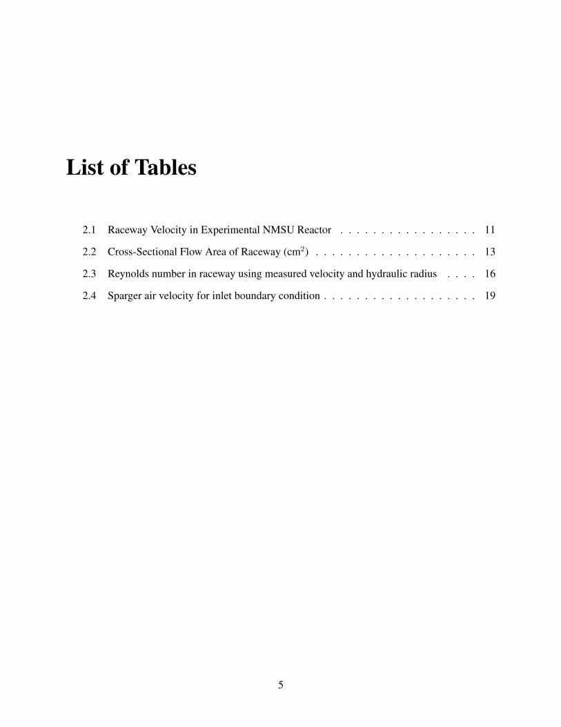
List of Tables
2.1 Raceway Velocity in Experimental NMSU Reactor . . . . . . . . . . . . . . . . . 11
2.2 Cross-Sectional Flow Area of Raceway (cm2) . . . . . . . . . . . . . . . . . . . . 13
2.3 Reynolds number in raceway using measured velocity and hydraulic radius . . . . 16
2.4 Sparger air velocity for inlet boundary condition . . . . . . . . . . . . . . . . . . . 19
5
Chapter 1
Literature Review
1.1 Introduction
Microalgae are a promising potential resource for a wide variety of uses. Interest in cultivation of
microalgae for food, lipids, pharmaceuticals, biofuels, carbon sequestration, and pollution mitiga-
tion has grown rapidly in recent years. Microalgae are photoautotrophs, and utilize photosynthesis
to convert solar energy into sugars for growth. Unlike higher plants, however, microalgae are sim-
ple aquatic organisms and do not need to maintain structural and resource-gathering components
such as stems, roots, and leaves. For this reason, microalgae have great potential for the mass
production of valuable resources.
Commercial cultivation of microalgae has occurred for over 40 years [14], however commercial
viability has been restricted mostly to high-value strains such as Spirulina for health food and
other supplements. Interest has grown in more recent years to cultivation of microalgae for use in
renewable fuels production, and although the technical feasibility of producing large amounts of
biofuels from algae is promising, the high cost of production compared to the relatively low price
of fuels remains an obstacle [10].
Significant challenges exist for the cultivation and harvest of microalgae. Algae have specific re-
6

quirements for light, CO2, temperature, and pH for optimal growth. In addition, other specific
requirements or nutrients may be required, depending on the species and the particular resource
for which it is grown. Large-scale algae cultivation may be conducted in open ponds or closed
photobioreactors, and each presents a unique set of unique benefits and disadvantages [11]. Closed
systems allow for greater control of nutrient, pH, and CO2 balance, and reduce the possibility
of contamination by native algae strains or other organisms. However, open pond systems are
much less expensive to build and maintain, which is an important consideration for fuels or sim-
ilar low-value products. Both approaches remain active areas of research in both academia and
industry.
1.1.1 Hydrodynamic and Fluid Characteristics
While the basic science of the growth requirements of various strains of microalgae is still being
explored to determine their potential for commercial cultivation, work must also continue to opti-
mize the engineering of large scale operations. Commercial algae cultivation as an industry may,
in some ways, be compared to the agriculture industry since both essentially involve using photo-
synthesis as a means of converting solar energy into useful products. However, unlike traditional
agriculture, which has thousands of years of history and development by mankind, large scale al-
gae cultivation has only been in development for a few decades at most, and there remain many
unknowns in the technical challenges involved in such systems.
Hydrodynamic and fluid characteristics of algae growth systems are important factors affecting
their success for a number of reasons. Algae must be maintained at proper pH, CO2, O2, and nutri-
ent balance for optimal growth. Since the algae are living organisms that consume these resources
and produced waste products from their metabolism, they interact and affect the environment they
live in. Any potential cultivation system must ensure that the algae experience adequate mixing
to ensure these conditions remain within the tolerance levels of the particular species being grown
in the system. In addition, algae require appropriate amounts of solar irradiation to provide the
7

energy required for photosynthesis. Dense cultures of algae may cause rapid attenuation of sun-
light with depth due to scattering by the water and absorption by the algae cells, so the region of
adequate solar irradiation is limited to the first few centimeters of growing medium. This places
limitations on the total depth and size of algae growth reactors. However, it has been shown that
optimal growth is obtained not necessarily by constant irradiation of direct sunlight, but rather by
the experience of a light/dark cycle by the individual cells [13]. Just as too little sunlight may result
in poor growth and death of algae cells, the algae may experience photoinhibition, in which they
experience poor growth or death due to too much sunlight. Finally, as algae are living organisms
they may be damaged under conditions of high shear, which may be a concern for systems utilizing
mechanical methods for circulation such as impellers or paddle wheels.
1.1.2 Computational Methods
All of the above mentioned factors are heavily influenced and in some cases may be controlled
by the fluid characteristics of an algae cultivation system, and optimization requires a thorough
investigation of these characteristics. As computational power has increased, computational fluid
dynamics (CFD) has emerged as a powerful tool in the analysis of complex fluid flows, including
research involving both closed and open bioreactors for algae growth [3]. This approach may allow
mixing characteristics, light access, and other important hydrodynamic factors to be investigated
without the need for full-scale construction of experimental photobioreactors (PBRs). Several
novel geometries have been studied using CFD methods, including torus shapes [8] and spiral
types [12] that have been shown to be improvements over traditional tubular PBR designs.
While the CFD approach is well-suited to analysis of the physical characteristics of fluid flow ,
it also may be combined with statistical methods to model the irradiation history of individual
cells, including consideration of light attenuation. Several methods have been considered or im-
plemented for this purpose, including a Beer-Lambert type relation or Monte Carlo simulation
[9]. Computational fluid dynamics may also be used to predict particle movement through a fluid
8

medium. This has important applications in optimization of algae growth systems, since it may
be used to track the potential movement of algae cells through the system. These methods have
been shown good agreement to experimental measurements in bubble column photobioreactors
[7]. Growth models may also be incorporated into CFD code as a predictive tool in investigations
related to the variation of fluid properties and their effects on the algae culture [5].
1.2 Objectives
The objective of this work is to implement a mathematical model of an airlift-driven raceway reac-
tor using computational fluid dynamics. Hydrodynamic and fluid characteristics are important in
reducing the energy requirements of algae growth systems while optimizing growth conditions, and
mathematical models can be powerful predictive tools utilized in the design of such systems.
The model developed here is based on experimental reactors developed and studied at New Mexico
State University [6]. In addition to creating a model that may be used to predict raceway velocity
under various operating regimes, the model will be used to predict the vertical mixing behavior in
a reactor of this type. A discrete phase model will be implemented to simulate the movement of a
sample of individual algae cells through this system and their positions recorded as they progress.
The results of the CFD simulation will then be compared to the vertical mixing behavior in a
straight-channel raceway configuration.
9
Chapter 2
Investigation of Airlift-Driven Raceway
2.1 Introduction
This chapter presents the methods used to investigate the flow characteristics of an airlift-driven
raceway reactor for algal cultivation. The investigation was based upon an experimental reactor
that has been developed at New Mexico State University. Data obtained from NMSU was used to
validate the CFD model presented here.
2.2 Experimental Configuration
Validation of the CFD model presented here was conducted by comparison to experimental mea-
surements of raceway velocity in an airlift-driven raceway reactor obtained by Ketheesan [6] at
New Mexico State University. The raceway section was composed of a semicircular section of
PVC pipe with an inner diameter of 14.5 cm. The airlift systems were fabricated from plexiglass
pipe of 6.875 cm inner diameter fitted with a center divider of width 1/10” (0.0254 cm). The center
divider extends down the length of the pipe to a distance of 6 cm from the bottom such that the pipe
functions as a U-tube with both downcomer and riser. The riser side of the pipe was fitted with
10

Table 2.1: Raceway Velocity in Experimental NMSU Reactor
Total Air Flow Reactor 1 Uncertainty Reactor 2 Uncertainty(mL/min) Velocity (cm/s) (+/- cm/s) Velocity (cm/s) (+/- cm/s)
1200 4.3523 0.0613 7.5171 0.13421600 5.2985 0.0906 8.2689 0.16212000 6.0932 0.1195 9.1876 0.19982400 6.4140 0.1322 10.3361 0.2521
rectangular 0.5′′ × 0.5′′ × 1.5′′ air spargers that produce the bubbles which drive the flow.
Two reactor configurations with different riser heights were evaluated in the experimental inves-
tigation at NMSU. The raceway sections were identical in both configurations, which consisted
of a smoothed rectangular arrangement 167.5 cm in length and 76 cm in width. Each reactor had
four airlift columns, positioned at the beginning and end of each of the longer raceway channels.
Reactor 1 had a riser height of 48 cm, and Reactor 2 had a riser height of 72 cm. For the liquid
circulation velocity tests, Reactor 1 was filled to a total volume of 20 L, and Reactor 2 was filled
to a total volume of 23 L.
In the experimental study, velocity in the raceway was determined using a tracer pulse injection
method for total airflow rates of 1200, 1600, 2000, and 2400 mL/min. Velocity measured in the
raceway for the four flow regimes is presented in Table 2.1.
2.3 CFD Methodology
2.3.1 Geometry
A 3D model of a proposed airlift-driven raceway reactor was developed using SolidWorks 2011-
2012. The model was developed as a single part containing the entire fluid region for the CFD
analysis at the same scale as the experimental NMSU reactor. Since the experimental reactor is
bilaterally symmetrical, only one-half of the system was modeled in SolidWorks to reduce compu-
11
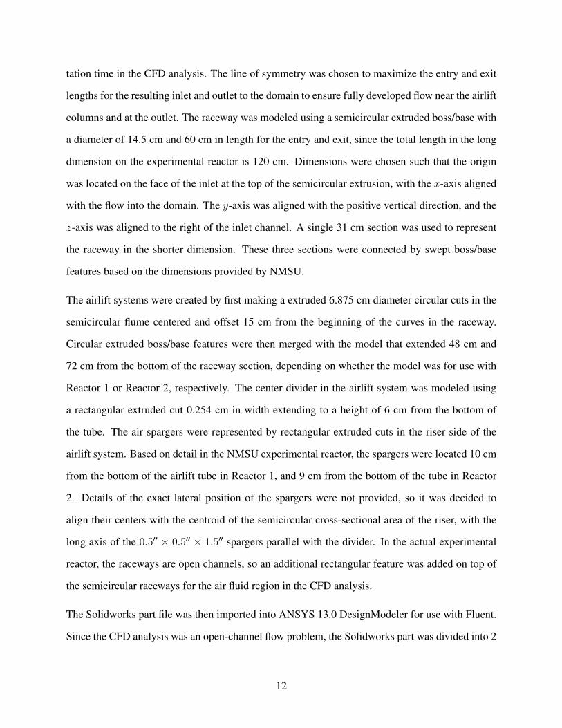
tation time in the CFD analysis. The line of symmetry was chosen to maximize the entry and exit
lengths for the resulting inlet and outlet to the domain to ensure fully developed flow near the airlift
columns and at the outlet. The raceway was modeled using a semicircular extruded boss/base with
a diameter of 14.5 cm and 60 cm in length for the entry and exit, since the total length in the long
dimension on the experimental reactor is 120 cm. Dimensions were chosen such that the origin
was located on the face of the inlet at the top of the semicircular extrusion, with the x-axis aligned
with the flow into the domain. The y-axis was aligned with the positive vertical direction, and the
z-axis was aligned to the right of the inlet channel. A single 31 cm section was used to represent
the raceway in the shorter dimension. These three sections were connected by swept boss/base
features based on the dimensions provided by NMSU.
The airlift systems were created by first making a extruded 6.875 cm diameter circular cuts in the
semicircular flume centered and offset 15 cm from the beginning of the curves in the raceway.
Circular extruded boss/base features were then merged with the model that extended 48 cm and
72 cm from the bottom of the raceway section, depending on whether the model was for use with
Reactor 1 or Reactor 2, respectively. The center divider in the airlift system was modeled using
a rectangular extruded cut 0.254 cm in width extending to a height of 6 cm from the bottom of
the tube. The air spargers were represented by rectangular extruded cuts in the riser side of the
airlift system. Based on detail in the NMSU experimental reactor, the spargers were located 10 cm
from the bottom of the airlift tube in Reactor 1, and 9 cm from the bottom of the tube in Reactor
2. Details of the exact lateral position of the spargers were not provided, so it was decided to
align their centers with the centroid of the semicircular cross-sectional area of the riser, with the
long axis of the 0.5′′ × 0.5′′ × 1.5′′ spargers parallel with the divider. In the actual experimental
reactor, the raceways are open channels, so an additional rectangular feature was added on top of
the semicircular raceways for the air fluid region in the CFD analysis.
The Solidworks part file was then imported into ANSYS 13.0 DesignModeler for use with Fluent.
Since the CFD analysis was an open-channel flow problem, the Solidworks part was divided into 2
12

Table 2.2: Cross-Sectional Flow Area of Raceway (cm2)
Configuration Experimental CFD Model
Reactor 1 31.58 31.582Reactor 2 23.68 23.685
bodies using a slice by plane operation in DesignModeler. This was done to improve the meshing
and post-processing for the liquid and gas regions in the CFD analysis. A new zx plane was added
to the model, offset -3.681 cm in the y direction from the origin for Reactor 1, and -4.335 cm for
Reactor 2. This plane represented the approximate level of the free surface, and was chosen so
that the resulting cross-sectional flow area of the raceway closely matched that of the experimental
reactor, as shown in Table 2.2.
2.3.2 Mesh
Meshing was performed using ANSYS 13.0 Meshing software. An automatic patch conform-
ing/sweeping method was chosen based on the CFD physics preference for the basic mesh with
only a few slight modifications from the default settings. The advanced size function was used
based on proximity and curvature, with the relevance center set to medium. Smoothing, transition,
and span angle center were set to medium, slow, and fine, respectively. Default settings were used
for curvature normal angle, number of cells across gap, minimum and maximum size of elements
and faces, and growth rate. Minimum edge size was set to 0.00254 m since this was the width of
the center divider in the airlift system.
Defeaturing was used to improve the mesh near the edges of the center divider. Since these were
in fact rectangular in shape with a face only 0.254 cm in width at the top and bottom, the initial
mesh resulted in elements with a very high skewness in these areas. Pinch tolerance was therefore
set to 0.003 m in order to eliminate these faces and the resulting high-skewness elements.
The resulting mesh for Reactor 1 consisted of 26,304 nodes and 124,032 elements, with a minimum
13
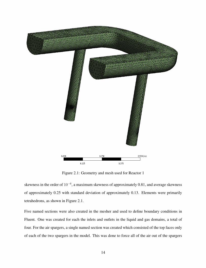
Figure 2.1: Geometry and mesh used for Reactor 1
skewness in the order of 10−6, a maximum skewness of approximately 0.81, and average skewness
of approximately 0.25 with standard deviation of approximately 0.13. Elements were primarily
tetrahedrons, as shown in Figure 2.1.
Five named sections were also created in the mesher and used to define boundary conditions in
Fluent. One was created for each the inlets and outlets in the liquid and gas domains, a total of
four. For the air spargers, a single named section was created which consisted of the top faces only
of each of the two spargers in the model. This was done to force all of the air out of the spargers
14

to be released from their top surfaces in the CFD simulations, reducing the total number of inlet
surfaces from 12 to 2 for the air. Moreover, with this assumption all of the air entering the system
is given an initial velocity in the direction of flow, which reduces the discretization needed around
the air spargers required to avoid a diverging solution. Although this is not entirely the case in
the experimental reactor, it was considered to be a reasonable assumption that would considerably
reduce computational time and improve convergence in the CFD analysis
2.3.3 Solver and Models
The CFD analysis was performed using ANSYS Fluent 13.0. Although the flow regimes investi-
gated represent quasi-steady conditions with constant airflow rates and relatively constant veloc-
ity in the raceway, the nature of the problem incorporating multiphase flow with a free surface
makes it impractical to achieve a steady state CFD solution. Therefore, a transient simulation was
performed using the pressure-based solver and gravitational acceleration set to -9.81 m/s2 in the
y-direction. For tracking the interface between the phases, the volume of fluid (VOF) model was
used with the open channel flow option enabled, which has been shown to an effective method
for multiphase flows when tracking a free surface is important [4]. It has also been shown to be
an effective model in CFD simulations of the hydrodynamics of bubble columns [1]. The explicit
scheme was used to calculate the volume fraction with implicit body force enabled. Since the ve-
locity measurements of the experimental reactor were performed using water as the working fluid,
air was chosen to be the primary phase and water was chosen as the secondary phase. However,
considering that even a dense algae culture contains a very small fraction of biomass, the use of
water to represent the heavier phase is a reasonable assumption for the intent and purpose of this
investigation. The choice of the heavier phase as the secondary phase is important for the open
channel flow options in the VOF model [2]. In order to accurately model the interface between the
air and water phases, a constant surface tension of 0.072 N/m was applied in the phase interaction
settings. A standard operating pressure of 101,325 Pa was applied, using a specified operating
15
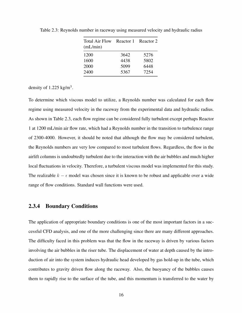
Table 2.3: Reynolds number in raceway using measured velocity and hydraulic radius
Total Air Flow Reactor 1 Reactor 2(mL/min)
1200 3642 52761600 4438 58022000 5099 64482400 5367 7254
density of 1.225 kg/m3.
To determine which viscous model to utilize, a Reynolds number was calculated for each flow
regime using measured velocity in the raceway from the experimental data and hydraulic radius.
As shown in Table 2.3, each flow regime can be considered fully turbulent except perhaps Reactor
1 at 1200 mL/min air flow rate, which had a Reynolds number in the transition to turbulence range
of 2300-4000. However, it should be noted that although the flow may be considered turbulent,
the Reynolds numbers are very low compared to most turbulent flows. Regardless, the flow in the
airlift columns is undoubtedly turbulent due to the interaction with the air bubbles and much higher
local fluctuations in velocity. Therefore, a turbulent viscous model was implemented for this study.
The realizable k − ε model was chosen since it is known to be robust and applicable over a wide
range of flow conditions. Standard wall functions were used.
2.3.4 Boundary Conditions
The application of appropriate boundary conditions is one of the most important factors in a suc-
cessful CFD analysis, and one of the more challenging since there are many different approaches.
The difficulty faced in this problem was that the flow in the raceway is driven by various factors
involving the air bubbles in the riser tube. The displacement of water at depth caused by the intro-
duction of air into the system induces hydraulic head developed by gas hold-up in the tube, which
contributes to gravity driven flow along the raceway. Also, the buoyancy of the bubbles causes
them to rapidly rise to the surface of the tube, and this momentum is transferred to the water by
16

friction and wake effects in the bubbles. While these interactions are complex, they can be resolved
and accounted for in the CFD solver with the appropriate boundary conditions and initial setup,
including a reasonable estimate of the final flow velocity.
Unfortunately, in the general case for problems of this type is that it is not known a priori what
the final flow velocity will be, since it is dependent on the air flow rate. One potential approach
would have been to model the entire reactor in the CFD analysis, initialize the domain with the
appropriate water level and beginning the transient simulation at the moment the air begins to
enter the system. This approach was considered inefficient as it would be very computationally
expensive due to the size of the domain, as well as potentially requiring a large number of time
steps to reach quasi-steady conditions. Therefore, the choice was made to split the domain in half
along the center line of symmetry, which reduced the size of the domain significantly and resulted
in definitive inlet and outlet boundary conditions for the raceway.
Raceway Inlets and Outlets
This approach did present some challenges in the decision of how to treat the inlets and outlets,
however. Velocity inlets, in which the fluid is given a specified velocity at the inlet, are typically
preferred for most CFD applications, however as stated earlier the raceway velocity in this type of
problem is not generally known prior to solving. Therefore, a pressure inlet boundary condition
with the open channel option selected was utilized for both the inlet in the water region as well
as the air region, with water selected as the secondary phase for the inlet. For Reactor 1, the free
surface level was specified to be -3.681 cm with the bottom level at -7.25 cm, which is the location
of the bottom of the raceway channel. For Reactor 2, the free surface level was specified to be
-4.335 cm with the bottom level also at -7.25 cm. Resulting inlet velocity was specified to be
normal to the boundary, with turbulence specified to be 10% intensity with a hydraulic diameter
of 8.3911 cm. These were considered to be reasonable assumptions since the inlet was far from
the airlift systems and the flow in this region should be stable and fully developed, and since the
17
volume of water in the system is not changing the free surface level should remain more or less
constant.
In addition to specifying the free surface level, the pressure inlet boundary condition requires input
regarding the energy added to the flow at the inlet. This can be given in the form of an upstream
velocity, or a total height specification. This presented a conundrum for the same reasons as the
velocity inlet boundary condition, since the inlet and outlet flow velocity is dependent on the
solution itself and therefore inappropriate to be used as a specified initial condition. Ultimately,
it was decided for the scope of this project to use the specified upstream velocity approach, and
utilize the measured experimental raceway velocities for each flow regime. However, this approach
put severe limitations on the general applicability of this CFD model, since it is limited to cases
for which there is already a well-known raceway velocity.
For the outlets in the raceway, a pressure outlet boundary condition with the open channel option
was used. The same turbulence settings as the inlets were used, with the backflow direction speci-
fied to be normal to the boundary. Also, the same settings were used in the open channel settings
with regard to the free surface and bottom levels. In the pressure outlet boundary condition, no
velocity specification is required.
Air Spargers
A velocity inlet was defined for the air spargers, which as stated earlier consisted of the upper faces
only of both spargers. Velocity was specified by magnitude normal to the boundary, and turbulence
intensity was specified to be 10% with a hydraulic diameter of 10.7 cm. Velocity was determined
for each flow regime based on the assumption that the volume flow rate for each flow regime was
divided evenly among the four spargers in the entire system, and the further assumption that all
of the air distributed to each sparger was released from the top surface only. Velocity was then
calculate by dividing the volume flow rate by the surface area of the top of the spargers. Velocity
calculations for each flow regime are summarized in Table 2.4.
18

Table 2.4: Sparger air velocity for inlet boundary condition
Total Air Flow Sparger Air Flow Sparger Air Flow Sparger Air Velocity(mL/min) (mL/min) (cm3/s) (cm/s)
1200 300 5 1.0331600 400 6.667 1.3782000 500 8.333 1.7222400 600 10 2.067
Other Boundaries
Other boundaries were considered to be stationary walls with a no-slip shear condition. Since the
actual experimental reactor was compose of PVC and plexiglass, the walls were treated as smooth.
It is worth noting that this boundary condition includes the upper surface of the domain. Although
in reality this surface is open to the atmosphere, a wall boundary condition was specified since
specification as an outlet would have a tendency towards divergence in the solution due to the
adjacent surfaces at the inlet are pressure inlets.
2.3.5 Solution Methods
The PISO scheme with default settings for skewness and neighbor correction was selected for
pressure-velocity coupling with the PRESTO scheme used for spatial discretization of pressure.
First order upwind schemes were used for momentum, turbulent kinetic energy, and turbulent
dissipation rate. These methods have been shown to be effective for CFD simulations of bubble
columns with the VOF multiphase model [1]. The geo-reconstruct scheme was chosen for the
volume fraction, and a first order implicit scheme was used for the transient formulation. Under-
relaxation factors for pressure, density, body forces, momentum, turbulent kinetic energy, turbulent
dissipation rate, and turbulent viscosity were 0.3, 1, 1, 0.7 0.8, 0.8, and 1, respectively.
In order to track the raceway velocity, volume flow rate, and mass balance as the solution pro-
gressed in time, a series of surface monitors were assigned to the relevant boundary conditions.
19

Raceway velocity was recorded using an area-weighted average surface integral of x-velocity at
the water inlet and water outlet boundary conditions. Similarly, volume flow rate was recorded at
these boundaries as well. Mass balance was calculated using a surface monitor of mass flow rate
at the water inlet and outlet, air inlet and outlet, and air sparger boundaries. These monitors were
calculated and written to a text file every 10 time steps.
At the beginning of the calculation, the solution was initialized by first filling the entire domain
with the air phase, then patching the water phase into the appropriate cells which lie below the
specified free surface level. No initial velocity was specified, and the entire system was assumed
to be rest. Calculation of the solution began at time t = 0 when the air spargers are first turned
on, and therefore were given the initial velocity conditions as specified in Table 2.4 for each flow
regime. This was a transient simulation using a fixed time step of 0.001 seconds. The maximum
iterations were time step was limited to 50.
2.3.6 Discrete Phase Model
One of the objectives of this project was to investigate the movement of individual algae cells
through the system to gain insight on the vertical mixing behavior important for the cells to
achieve an adequate light/dark cycle for their growth. To accomplish this, a discrete phase model
(DPM) was employed after the simulation had run for enough time to achieve quasi-steady condi-
tions.
Due to the transient nature of the problem, unsteady particle tracking was selected for the DPM,
where the particles were tracked with the fluid flow time step. Since the size of most algae cells
are very small, and have a similar density to water, the DPM was kept simple by assumption of the
cells as spherical particles of 10 µm in diameter with a density of 998.2 kg/m3.
From observations of raceway velocity recorded in the surface monitors, quasi-steady conditions
were observed after approximately 20 seconds of flow time in Reactor 1, so it was decided to begin
20
the DPM tracking at 30 seconds of flow time. A single surface injection was made at this time by
specifying an injection start time of 30.000 seconds and stop time of 30.001 seconds.
By default, Fluent only displays the current position of particles in the unsteady discrete phased
model. Since we were interested in tracking the position of the particles as they moved through the
domain over time, a user defined function (UDF) was employed to record the position and velocity
of each particle every 100 time steps (0.1 s flow time) and write the information to a text file for
postprocessing.
2.4 Results and Discussion
2.4.1 Raceway Velocity
Since the flow for this problem is quasi-steady at best, it could not be assumed that the velocity
recorded by the surface integral monitors at the inlets and outlets for any particular time step was
an accurate representation of the measured velocity in the experimental reactor. Therefore, a time-
averaged raceway velocity was determined by calculating the mean velocity after quasi-steady
conditions were reached.
As indicated in Figures 2.2, 2.3, 2.4, and 2.5, strongly oscillating flow is observed after the intro-
duction of air from the spargers during the first 15 seconds of flow time for both reactor configu-
rations under all of the air flow rates investigated. While this could be result of the time required
for convergence of the numerical solution, it is also a physically realistic result due to the sudden
introduction of energy into the system and the resulting change in momentum of the water. Re-
gardless, the simulation was considered to have reached quasi-steady conditions after 20 seconds
of flow time for all configurations and flow regimes.
To determine a predicted bulk flow velocity in the raceway from the CFD results, an average
velocity at the inlet and outlet was calculated using the mean area-weighted average surface integral
21

Figure 2.2: Reactor 1 area-weighted average x-velocity at inlet
Figure 2.3: Reactor 1 area-weighted average x-velocity at outlet
22
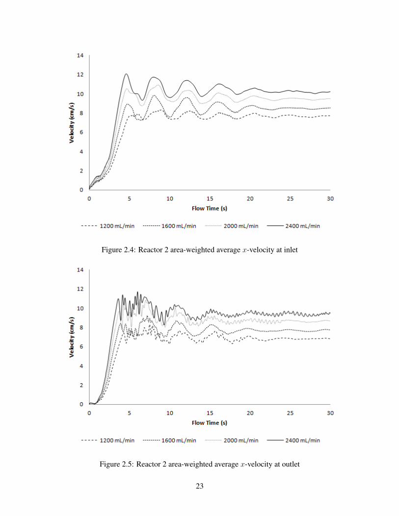
Figure 2.4: Reactor 2 area-weighted average x-velocity at inlet
Figure 2.5: Reactor 2 area-weighted average x-velocity at outlet
23

of x-velocity at the water-inlet and water-outlet boundary conditions over a 10 second time period,
beginning at time step 20000 (20 s flow time). Since these boundary conditions were defined by
the specified free surface level of the water, and a significant entry and exit length was available
for the inlet and outlet boundaries, respectively, it can be assumed that the area-weighted surface
integral over these surfaces provide an accurate representation of the bulk velocity of the water in
the raceway.
Using this approach, the predicted velocity in Reactor 1 showed good agreement with experimental
measurements, especially when calculated from the inlet boundary, as shown in Figure 2.6. Error
bars indicate the uncertainty in the experimental measurements for each flow regime, and the
predicted velocity calculated is near or within the experimental uncertainty. However, it should
be noted that predicted velocity from the outlet boundary condition was significantly different
than that predicted at the inlet. Moreover, whereas the velocity predicted the inlet boundary was
greater than the experimental measurements, the velocity predicted at the outlet was less than the
experimental measurements for all flow regimes, and fell outside the range of uncertainty, as shown
in Figure 2.7.
Predictions for Reactor 2 did not match the experimental measurements quite as well as those
for Reactor 1. Again, the velocity predicted using the inlet boundary tended to be higher than the
experimental measurements, with a notable exception at air flow rates of 2400 mL/min. At this flow
regime, the velocity predicted at the inlet was slightly lower than the experimental measurements,
and within the range of uncertainty of those measurements, as indicated in Figure 2.8. Velocity
predicted using the outlet boundary was consistently lower than the experimental measurements,
as shown in Figure 2.9.
2.4.2 Particle Tracking
The unsteady discrete phase model (DPM) was employed in the Reactor 1 study for air flow rates
of 1600 mL/min and 2400 mL/min to to simulate the movement algae through the reactor. The
24
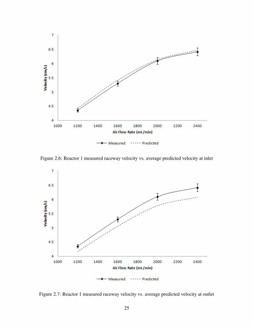
Figure 2.6: Reactor 1 measured raceway velocity vs. average predicted velocity at inlet
Figure 2.7: Reactor 1 measured raceway velocity vs. average predicted velocity at outlet
25
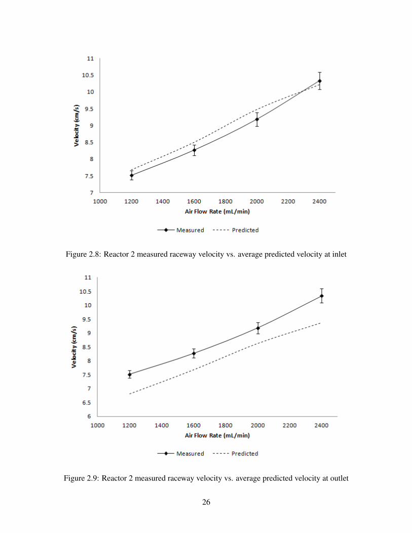
Figure 2.8: Reactor 2 measured raceway velocity vs. average predicted velocity at inlet
Figure 2.9: Reactor 2 measured raceway velocity vs. average predicted velocity at outlet
26

particles were released as a single surface injection at 30 seconds flow time and tracked for an
additional 30 seconds of flow time. Position and velocity were recorded every 100 time steps (0.1
s) with a UDF. The surface injection method places one particle per face at the chosen surfaces
and automatically assigns an ID number to each particle, which was used by the UDF to track
each unique particle through the domain. A selection of 8 particles from the the DPM results were
then chosen based on initial vertical and horizontal position to represent the general behavior of the
algae. The main parameter of interest in this study was the vertical mixing intensity experienced by
the algae cells as they move through the raceway, since that is an important factor in determining
whether or not each cell receives an equal and adequate amount of solar irradiance required for
their growth.
As indicated in the y-position history plots shown in Figures 2.10 and 2.11, a significant amount
of vertical movement is experienced by all of the representative particles as they move through
the inlet channel, the airlift column, and then through the U-shaped section of the raceway. In
both flow regimes, the plots suggest that the particles generally move towards the surface as they
approach the downcomer of the bubble column at about 35 seconds of flow time, then spend a few
seconds near the surface as they come out of the riser tube between about 42-45 seconds flow time.
After this they tend to show random behavior as some of them move towards the bottom again,
others stay near the top, while others exhibit an oscillatory behavior between about 45-60 seconds
flow time. This behavior is indicative of the turbulent conditions induced by the bubble columns
and the rapid shift in momentum experienced by the water as it moves from the riser tube back
to the raceway. Since the behavior of an arbitrary particle in this simulation is rather chaotic and
random, it can be assumed that vertical mixing does indeed take place in this configuration, and
when utilized in an algae cultivation system will lead to adequate and equal solar irradiation for
the algae cells over time.
27
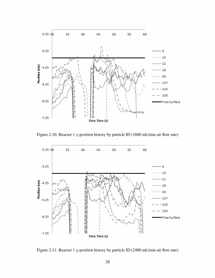
Figure 2.10: Reactor 1 y-position history by particle ID (1600 mL/min air flow rate)
Figure 2.11: Reactor 1 y-position history by particle ID (2400 mL/min air flow rate)
28
2.5 Limitations
The CFD model presented here does a fairly acceptable job of matching the experimental flow
conditions, as illustrated in the raceway velocity study. However, it required input from the experi-
mental measurements as initial conditions. It is not known how accurately the model would predict
the flow conditions without such a well known initial guess so close to the final result. Therefore,
it cannot be assumed that this model will be applicable to scenarios where the raceway velocity
is not well known. This places severe limitations on the broader application of this model as a
predictive tool for other configurations and flow regimes. Such scenarios may include changes in
geometry or flow rate. A more robust model which utilizes an adaptive upstream velocity at the
boundary condition as opposed to a constant upstream velocity, for example, may be required for
use in such studies.
29

Chapter 3
Investigation of Straight-Channel
Raceway
3.1 Introduction
Typically, open raceway reactors are driven by paddlewheel systems to provide the circulation re-
quired to keep the algae cells in suspension. The use of airlift pumps has been shown by Ketheesan
[6] to be a more energy efficient method to achieve adequate flow velocity in the raceway. How-
ever, there may be other benefits to this approach which have not yet been explored. One of the
primary objectives of this study was to compare the vertical mixing behavior in an airlift-driven
raceway compared to a traditional paddlewheel-driven system, since this is an important factor
affecting the overall productivity of open algae cultivation systems. Therefore, a comparison study
was performed of a simple straight-channel open raceway reactor, without the airlift system, but
otherwise of the same dimensions as the study presented in Chapter 2. While this is not a complete
representation of a paddlewheel driven system, since a paddlewheel would have its own unique
dynamic characteristics and turbulence it would add to the flow, it does provide a basic example of
fluid movement through a raceway channel for comparison.
30
3.2 CFD Methodology
3.2.1 Geometry
The same Solidworks model that was used for the airlift-driven reactors was used for the straight-
channel study, the only difference was that the airlift columns were removed and the channel had
a smooth bottom throughout its length. The Solidworks model was then imported into ANSYS
DesignModeler and divided into a two-body part at y = −3.681 using a similar technique as
described for the airlift-driven system.
3.2.2 Mesh
Since the straight-channel raceway contained much simpler geometry than the airlift driven race-
way model, the meshing was more straightforward. The same settings were used as those used in
the airlift raceway, except there was no need for advanced defeaturing and pinch controls. The re-
sulting automatic meshing method resulted in a swept mesh of 11,076 nodes and 8,883 elements,
primarily hexahedrons as seen in Figure 3.1. Minimum skewness was in the order of 10−5, the
maximum was about 0.39, and the average was about 0.10 with a standard deviation of about
0.11.
3.2.3 Boundary Conditions
The solver and models used for the CFD analysis were essentially the same as those used for the
airlift pump study. The only difference were the boundary conditions, Since there are no airlift
columns and the associated air-inlet boundary to add momentum and drive the flow, the pressure
inlet boundary condition would have resulted in low or zero flow velocity and was inappropriate to
use in this case. A velocity inlet boundary condition was chosen instead. Two different cases were
investigated in which the inlet velocity was specified as 5.30 cm/s and 6.41 cm/s, representing
31

Figure 3.1: Geometry and mesh used for straight-channel raceway study
the 1600 mL/min and 2400 mL/min airflow rates in the previous study, respectively. Both inlet
boundaries for the air and water regions were given the initial velocity, with the specification of
the volume fraction of the water phase in the two regions to be 0 and 1, respectively. A pressure
outlet with the open channel option and specified free surface level at -3.681 cm was used for the
outlet boundary condition.
3.2.4 Solution Methods
The solution was initialized in a similar manner as was used for the airlift-driven raceway study.
However, to aid convergence and reduce the computational time, most of the domain was given an
initial velocity equal to that of the inlet boundary condition. This was done by patching the appro-
priate velocity into the cells below the free surface level and within 3 distinct regions containing the
straight sections of the channel. The inlet region was given a velocity in the positive x-direction,
the region perpendicular to this was given an initial velocity in the negative z-direction, and the
outlet region was given a velocity in the negative x-direction. The curved sections were simply
left static, which did lead to somewhat increased convergence time in the first few time steps, but
32
overall this initialization seemed effective in reducing the total time required to solve.
3.2.5 Discrete Phase Model
A discrete phase model was employed for particle tracking in this study. Methods and settings
were identical to those described in Chapter 2.
3.3 Results and Discussion
3.3.1 Flow Rate
The area-weighted velocity at the inlet and outlet boundaries were monitored as they were in the
airlift-driven reactor study. Since the inlet boundary velocities were specified, these values were
constant, but the outlet velocity displayed an oscillatory behavior in the transient simulation as
seen in Figures 3.2 and 3.3. Even with the initialization procedure described above, this oscillatory
behavior was seen for a much longer duration of flow time than occurred for the airlift-driven
raceway study, even as long as 60 seconds flow time which was the maximum runtime of the
simulations. Nevertheless, the outlet velocity did seem to be converging towards the specified inlet
velocity, at least in the 5.30 cm/s case as seen in Figure 3.2. The 6.41 cm/s case did not show quite
as good of agreement between the inlet and outlet velocity, and appeared to be converging toward
a slightly reduced velocity at the outlet, as can be seen in Figure 3.3.
3.3.2 Particle Tracking
Particle tracking results from the DPM were noticeably different than those for the airlift-driven
study for both velocity cases investigated. Particles were tracked for 30 seconds of flow time,
which is approximately the time required for them to pass through the entire raceway channel if
33

Figure 3.2: Straight-channel inlet/outlet velocity convergence history (5.30 cm/s flow rate)
Figure 3.3: Straight-channel inlet/outlet velocity convergence history (6.41 cm/s flow rate)
34

moving through the centerline at the bulk raceway velocity for the two cases study, although the
average time required would understandably be slightly greater for the 5.30 cm/s case than for the
6.41 cm/s case since the bulk velocity is lower.
Select particles were plotted by particle ID in Figures 3.4 and 3.5. Very little vertical movement
was seen for at least the first 10 seconds after the particles were injected, between 30-40 seconds
flow time. The greatest vertical movement was seen between about 40-50 seconds of flow time
before the particles tended to stabilize somewhat for the last 10 seconds of tracking. This may
be due to mixing caused by the geometry of the reactor, as the particles moved through the the
U-shaped section of the raceway.
Of particular interest is the noticeable separation of the particles into two general trajectories. With
a few exceptions, particles initially near the surface tended to stay near the surface, and those near
the bottom tended to remain close to the bottom. This suggests that in this particular configuration,
vertical turnover is not prone to occur, which may lead to uneven distribution of solar irradiance
among individual algae cells in an algae cultivation reactor of this type. It is also observed that for
the most part, the particles near the surface tend to experience more vertical movement than those
near the bottom. This is to be expected since the flow regime, although slightly turbulent overall,
may still contain regions of laminar-type flow, particularly close to the walls due to the no-slip
boundary condition.
3.4 Limitations
While this study does present a general comparative model illustrating the general behavior of par-
ticles through a smooth, straight-channel raceway under under the flow conditions investigated, it
falls short of being a thorough investigation the behavior in a paddlewheel-driven raceway reactor.
The inlet velocity boundary condition was treated as constant and uniform with very little initial
turbulence. This is not an accurate representation of the initial conditions provided by an actual
35

Figure 3.4: Straight-channel y-position history by particle ID (5.30 cm/s flow rate)
Figure 3.5: Straight-channel y-position history by particle ID (6.41 cm/s flow rate)
36

paddlewheel moving through the water, which imparts not only a horizontal momentum but also
a vertical momentum as the angle of the blades change. Accurate mathematical modeling of this
type of configuration would be better accomplished by incorporating a sliding or dynamic mesh to
represent the paddle blades, and is beyond the scope of this study.
37

Chapter 4
Conclusions and Future Work
This study presented a mathematical model of an airlift-driven raceway reactor using computa-
tional fluid dynamics. The model was used to predict the velocity in the raceway channel and
compared to experimental measurements of a similar reactor. The model was then used to predict
the vertical mixing behavior in a reactor of this type, and to gain insight on the vertical movement
of individual algae cells as they move through the reactor using a discrete phase model, which was
then compared to the vertical mixing behavior in a straight channel raceway configuration.
Raceway velocity predictions showed relatively good agreement to experimental measurements,
although as stated in Section 2.3.4 the accuracy of the solution is likely to be highly dependent on
the accuracy of the initial guess of the velocity upstream of the pressure inlet. Future work may
include a more robust model capable of adapting this upstream velocity to fit the solution as it
progresses through time steps. This could likely be accomplished rather easily with a user defined
function (UDF) that updates the upstream velocity value at the current time step to match the
predicted outlet velocity at the previous time step. Due to the symmetry condition employed by this
study, these velocity profiles should technically be the same, so this approach should improve the
accuracy of the model, although some experimentation may be required to determine the specific
algorithm that would result in convergence of the predicted velocity.
38
In this preliminary study, the airlift-driven reactor does show improved vertical mixing behavior
over the straight-channel reactor. However, several improvements may be made to the models
used for particle tracking in both configurations. Due to the relatively low Reynolds number of
the raceway flow in all of the configurations here, a turbulent dispersion model was not employed
in the discrete phase model, since this may lead to non-physical results for these types of flows.
However, in the absence of a turbulent dispersion model a finer discretization is recommended
for the raceway regions in order to improve the accuracy of the particle tracks. In addition, a
number of recommendations may be made to the straight-channel reactor study in order to more
accurately model the mixing behavior in a paddlewheel driven reactor, including the incorporation
of a sliding-mesh model as described in Section 3.4.
39

Bibliography
[1] A. Akhtar. Cfd simulations for continuous flow of bubbles through gas-liquid columns: Ap-plication of vof method. Chemical Product and Process Modeling, 2(1):1–19, 2007.
[2] ANSYS 13.0. Fluent User’s Guide, ANSYS Inc.
[3] J.P. Bitog, I.-B. Lee, C.-G. Lee, K.-S. Kim, H.-S. Hwang, S.-W. Hong, I.-H. Seo, K.-S.Kwon, and E. Mostafa. Application of computational fluid dynamics for modeling and de-signing photobioreactors for microalgae production: A review. Computers and Electronicsin Agriculture, 76(2):131 – 147, 2011.
[4] C.W. Hirt and B.D. Nichols. Volume of fluid (vof) method for the dynamics of free bound-aries. Journal of computational physics, 39(1):201–225, 1981.
[5] S.C. James and V. Boriah. Modeling algae growth in an open-channel raceway. Journal ofComputational Biology, 17(7):895–906, 2010.
[6] B. Ketheesan and N. Nirmalakhandan. Development of a new airlift-driven raceway reactorfor algal cultivation. Applied Energy, 2011.
[7] H.P. Luo and M.H. Al-Dahhan. Verification and validation of cfd simulations for local flowdynamics in a draft tube airlift bioreactor. Chemical Engineering Science, 66(5):907–923,2011.
[8] J. Pruvost, L. Pottier, and J. Legrand. Numerical investigation of hydrodynamic and mixingconditions in a torus photobioreactor. Chemical engineering science, 61(14):4476–4489,2006.
[9] R. Rosello Sastre, Z. Csögör, I. Perner-Nochta, P. Fleck-Schneider, and C. Posten. Scale-down of microalgae cultivations in tubular photo-bioreactors–a conceptual approach. Journalof biotechnology, 132(2):127–133, 2007.
[10] J. Sheehan et al. A look back at the US Department of Energy’s Aquatic Species Program:Biodiesel from algae, volume 328. National Renewable Energy Laboratory Golden, CO,1998.
[11] C.U. Ugwu, H. Aoyagi, and H. Uchiyama. Photobioreactors for mass cultivation of algae.Bioresource Technology, 99(10):4021 – 4028, 2008.
[12] LB Wu and YZ Song. Numerical investigation of flow characteristics and irradiance historyin a novel photobioreactor. African Journal of Biotechnology, 8(18), 2010.
40
[13] X. Wu and J.C. Merchuk. A model integrating fluid dynamics in photosynthesis and photoin-hibition processes. Chemical Engineering Science, 56(11):3527–3538, 2001.
[14] L. Xu, P.J. Weathers, X.R. Xiong, and C.Z. Liu. Microalgal bioreactors: Challenges andopportunities. Engineering in Life Sciences, 9(3):178–189, 2009.
41
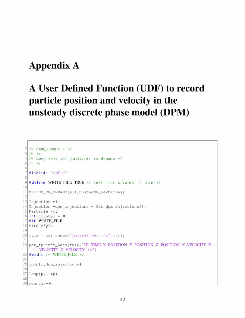
Appendix A
A User Defined Function (UDF) to recordparticle position and velocity in theunsteady discrete phase model (DPM)
12 / * dpm_sample . c * /3 / * * /4 / * Loop ove r a l l p a r t i c l e s i n domain * /5 / * * /67 # i n c l u d e " udf . h "89 # d e f i n e WRITE_FILE TRUE / * t e x t f i l e c r e a t e d i f t r u e * /
1011 DEFINE_ON_DEMAND (all_unsteady_particles )12 {13 Injection *I ;14 Injection *dpm_injections = Get_dpm_injections ( ) ;15 Particle *p ;16 i n t counter = 0 ;17 # i f WRITE_FILE18 FILE *fyle ;1920 fyle = par_fopen ( " p a r c e l s . o u t " , " a " , 1 , 1 ) ;2122 par_fprintf_head (fyle , " ID TIME X−POSITION Y−POSITION Z−POSITION X−VELOCITY Y←↩
−VELOCITY Z−VELOCITY \ n " ) ;23 # e n d i f / * WRITE_FILE * /2425 loop (I ,dpm_injections )26 {27 loop (p ,I−>p )28 {29 counter++;
42
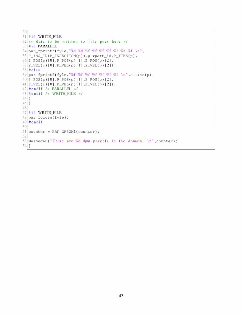
3031 # i f WRITE_FILE32 / * d a t a t o be w r i t t e n t o f i l e goes h e r e * /33 # i f PARALLEL34 par_fprintf (fyle , "%d %d %f %f %f %f %f %f %f \ n " ,35 P_INJ_ID (P_INJECTION (p ) ) ,p−>part_id ,P_TIME (p ) ,36 P_POS (p ) [ 0 ] ,P_POS (p ) [ 1 ] ,P_POS (p ) [ 2 ] ,37 P_VEL (p ) [ 0 ] ,P_VEL (p ) [ 1 ] ,P_VEL (p ) [ 2 ] ) ;38 # e l s e39 par_fprintf (fyle , "%f %f %f %f %f %f %f \ n " ,P_TIME (p ) ,40 P_POS (p ) [ 0 ] ,P_POS (p ) [ 1 ] ,P_POS (p ) [ 2 ] ,41 P_VEL (p ) [ 0 ] ,P_VEL (p ) [ 1 ] ,P_VEL (p ) [ 2 ] ) ;42 # e n d i f / * PARALLEL * /43 # e n d i f / * WRITE_FILE * /44 }45 }4647 # i f WRITE_FILE48 par_fclose (fyle ) ;49 # e n d i f5051 counter = PRF_GRSUM1 (counter ) ;5253 Message0 ( " There a r e %d dpm p a r c e l s i n t h e domain . \ n " ,counter ) ;54 }
43