INVESTIGATION OF CORROSION OF MSE WALLS IN NEVADA

INVESTIGATION OF CORROSION OF MSE WALLS IN NEVADA

Final Report to:

NEVADA DEPARTMENT OF TRANSPORATION

1263 South Stewart Street

Carson City, Nevada 89712

by:

Raj V. Siddharthan, Ph.D., P.E.

John Thornley, M.S.

and

Barbara Luke, Ph.D., P.E.

Research Report No. 2010-01

September 2010

UNIVERSITY OF NEVADA, RENO

Geotechnical Engineering Program Department of Civil and

Environmental Engineering

College of Engineering

University of Nevada

Reno, Nevada 89557

ii

Abstract

Nevada has over 150 mechanically stabilized earth (MSE) retaining walls at 39

locations. Recently, high levels of corrosion were observed due to accidental discovery

at two of these locations, specifically I-515/Flamingo Road and I-15/Cheyenne Avenue

intersections. The resulting investigations of these walls produced direct measurements

regarding the corrosion losses of the soil reinforcements, which included both bare steel

and galvanized steel and electrochemical properties of the MSE backfill in order to

identify its aggressiveness. One of the three walls at the Flamingo intersection was

replaced with a cast-in-place tie-back wall at great expense because of the significant

metal loss due to corrosion. The initial Flamingo investigation focused on average

uniform corrosion loss values from the direct reinforcement measurements and laboratory

backfill test results based on a variety of test methods. The investigation results are

reevaluated in this report, through the incorporation of statistical analysis in order to

effectively undertake a prediction that includes the variability in electrochemical

properties.

The investigation found that the original MSE backfill approval test results are

significantly different from those measured in the subsequent investigations. A

correlation has been developed between two distinctly different soil resistivity laboratory

test methods, namely the Nevada T235B and AASHTO T-288 methods. The Nevada test

method under predicts the corrosive nature of backfill soils when compared to the

AASHTO test method. A Nevada test predicting mildly corrosive backfill would be

iii

evaluated as corrosive using the AASHTO procedure. As the Flamingo and Cheyenne

investigations show, this has proved detrimental to the service lives of MSE structures.

The internal stability analysis of the two remaining MSE walls at the Flamingo

intersection were also analyzed using corrosion loss models developed from the statistical

analysis of the direct measurements. The results of the analysis from these two

intersections were subsequently extrapolated to other Nevada MSE walls. Through

review of the backfill approval data, specific Nevada MSE walls have been ranked

relative to estimated backfill aggressiveness and specific suggestions for future corrosion

analysis are recommended. There are four groups of evaluation methods that have been

identified in this research. Each of these methods has its own usefulness, but some will

be more costly than others. The four groups of evaluation methods for existing walls

include representative backfill soil testing, installation of non-stressed soil

reinforcements, nondestructive monitoring methods, and destructive direct observational

methods.

iv

Acknowledgements

First and foremost, I would like to give special thanks to my wife Jean, who has

been so supportive of my educational endeavors. I would also like to thank my advisor,

Raj Siddharthan, whose patience, guidance, and direction have helped me develop a more

fundamental understanding of critical engineering concepts. Gary Norris, with his love

of teaching and deep understanding of soil behavior, has been a great mentor as well.

Special thanks are also due to George Fernandez, for his assistance in statistical analysis

methods.

I would also like to thank the personnel at the Nevada Department of

Transportation for their assistance in this research. Those who deserve specific attention

include J. Mark Salazar, Abbas Bafghi, Todd Stefonowicz, and William Blake. In

addition, our sincere thanks are due to other research panel members, Daniel Alzamora,

Roma Clewell, Cole Mortensen, David Mrowiec, Terry Philbin and Jason Van Havel for

their valuable input. Without their insight and contribution this research would not be as

complete or as useful for future work.

v

Table of Contents

1.0 Introduction .................................................................................................................1

1.1 Project Information ....................................................................................................4

1.1.1 Scope of Project ...................................................................................................4

1.2 Organization of the Report .........................................................................................5

2.0 Historical Background................................................................................................7

2.1 Historical Corrosion Studies ......................................................................................7

2.1.1 National Bureau of Standards Circular 579 .........................................................8

2.1.2 Reinforced Earth Company Study .......................................................................9

2.2 Historical Field Investigations .................................................................................11

2.2.1 Caltrans 14 Wall Study ......................................................................................11

2.2.2 South African Wall Study .................................................................................13

2.2.3 Flamingo Wall Study .........................................................................................14

2.3 Soil Reinforcement Corrosion Surveys ....................................................................16

2.3.1 AMSE Survey ....................................................................................................17

2.3.2 NCHRP Survey .................................................................................................19

2.3.3 Oregon Department of Transportation Survey ..................................................21

2.4 Soil Reinforcement Corrosion Recommendations and Practices .............................22

2.4.1 Early Years ........................................................................................................23

2.4.2 FHWA ...............................................................................................................24

2.4.3 AASHTO ...........................................................................................................26

2.4.4 Nevada Department of Transportation ..............................................................28

2.4.5 Local States .......................................................................................................30

3.0 Corrosion Background .............................................................................................32

3.1 Corrosion of Buried Steel .........................................................................................32

3.1.1 Corrosion Mechanisms ......................................................................................32

3.1.2 Corrosive Measures of Backfill .........................................................................37

3.1.3 Estimated Corrosion Rates ................................................................................37

vi

3.2 Summary of Electrochemical Testing Methods .......................................................40

3.2.1 Soil Resistivity...................................................................................................41

3.2.1.1 Soil Resistivity Correlation ........................................................................44

3.2.2 Soluble Salts ......................................................................................................47

3.2.2.1 Chloride Content ........................................................................................47

3.2.2.2 Sulfate Content ...........................................................................................49

3.2.3 Soil pH ...............................................................................................................51

4.0 Nevada Case Studies .................................................................................................53

4.1 Flamingo Walls ........................................................................................................53

4.1.1 Field Investigation .............................................................................................55

4.1.1.1 Information Collected ................................................................................56

4.1.1.2 Testing Results ...........................................................................................57

4.1.1.3 Flamingo Field Investigation Conclusions .................................................58

4.1.2 Further Analysis of Data Collected ...................................................................59

4.1.2.1 Corrosion Rates from Direct Diameter Measurements ..............................60

4.2.2.2 Evaluation of Backfill.................................................................................65

4.1.2.2.1 Statistical Evaluation of Soil Resistivity Test Results ........................69

4.1.2.2.2 Statistical Evaluation of Chloride Content Test Results .....................71

4.1.2.2.3 Statistical Evaluation of Sulfate Content Test Results ........................72

4.1.2.2.4 Statistical Evaluation of pH Test Results ............................................72

4.1.2.3 Potential Effects on Wall Stability .............................................................73

4.2 Cheyenne Wall Study ...............................................................................................78

4.2.1 Sampling and Measuring of Soil Reinforcements .............................................81

4.2.2 Cheyenne Analysis – Soil Reinforcements .......................................................82

4.2.2.1 Estimated Corrosion Rate ...........................................................................83

4.2.3 Cheyenne Analysis – Backfill Soils ..................................................................85

4.2.3.1 Statistical Evaluation of Soil Resistivity Test Results ...............................86

4.2.3.2 Statistical Evaluation of Chloride Content Test Results ............................87

4.2.3.3 Statistical Evaluation of Sulfate Content Test Results ...............................87

vii

4.2.3.4 Statistical Evaluation of pH Test Results ...................................................87

4.2.4 Further Evaluation of Cheyenne Walls .........................................................88

4.3 Concluding Remarks Regarding Both Case Studies ................................................88

5.0 Nevada MSE Wall Database Development.............................................................90

5.1 MSE Wall Data Collection .......................................................................................90

5.1.1 Information Collected ........................................................................................92

5.1.2 MSE Wall Database ..........................................................................................97

5.1.3 Materials Testing Spreadsheets .......................................................................101

5.2 Limitations of Data Collection ...............................................................................103

6.0 Prediction of Corrosion Behavior of Other Nevada MSE Walls ........................104

6.1 Evaluation of Historical Nevada MSE Backfills ....................................................104

6.2 Methods for Future Evaluation of Existing MSE Walls ........................................111

6.2.1 Representative Backfill Soil Testing ...............................................................111

6.2.2 Installation of Non-Stressed Soil Reinforcements ..........................................114

6.2.3 Nondestructive Monitoring Methods ..............................................................115

6.2.4 Destructive Direct Observational Methods .....................................................116

6.3 Future MSE Wall Investigation Recommendations ...............................................117

7.0 Conclusion and Recommendations .......................................................................119

Recommendations ........................................................................................................121

References .......................................................................................................................124

Appendix A .....................................................................................................................207

viii

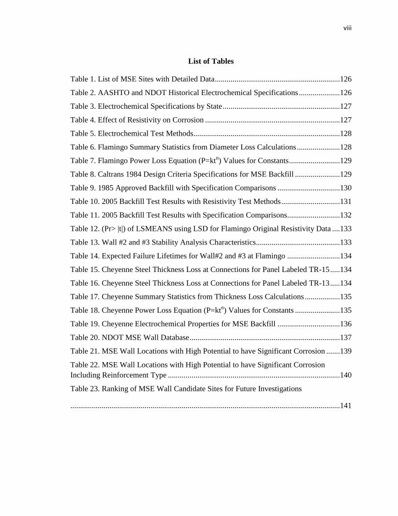
List of Tables

Table 1. List of MSE Sites with Detailed Data ................................................................126

Table 2. AASHTO and NDOT Historical Electrochemical Specifications .....................126

Table 3. Electrochemical Specifications by State ............................................................127

Table 4. Effect of Resistivity on Corrosion .....................................................................127

Table 5. Electrochemical Test Methods ...........................................................................128

Table 6. Flamingo Summary Statistics from Diameter Loss Calculations ......................128

Table 7. Flamingo Power Loss Equation (P=ktn) Values for Constants ..........................129

Table 8. Caltrans 1984 Design Criteria Specifications for MSE Backfill .......................129

Table 9. 1985 Approved Backfill with Specification Comparisons ................................130

Table 10. 2005 Backfill Test Results with Resistivity Test Methods ..............................131

Table 11. 2005 Backfill Test Results with Specification Comparisons...........................132

Table 12. (Pr> |t|) of LSMEANS using LSD for Flamingo Original Resistivity Data ....133

Table 13. Wall #2 and #3 Stability Analysis Characteristics ...........................................133

Table 14. Expected Failure Lifetimes for Wall#2 and #3 at Flamingo ...........................134

Table 15. Cheyenne Steel Thickness Loss at Connections for Panel Labeled TR-15 .....134

Table 16. Cheyenne Steel Thickness Loss at Connections for Panel Labeled TR-13 .....134

Table 17. Cheyenne Summary Statistics from Thickness Loss Calculations ..................135

Table 18. Cheyenne Power Loss Equation (P=ktn) Values for Constants .......................135

Table 19. Cheyenne Electrochemical Properties for MSE Backfill ................................136

Table 20. NDOT MSE Wall Database .............................................................................137

Table 21. MSE Wall Locations with High Potential to have Significant Corrosion .......139

Table 22. MSE Wall Locations with High Potential to have Significant Corrosion

Including Reinforcement Type ........................................................................................140

Table 23. Ranking of MSE Wall Candidate Sites for Future Investigations

..........................................................................................................................................141

ix

List of Figures

Figure 1. MSE Wall Located at South McCarran and I-80 .............................................142

Figure 2. Equivalence in Resistivity of Soluble Salts ......................................................143

Figure 3. Distribution of pH Measurements for MSE Backfills in the AMSE Survey ...144

Figure 4. AASHTO Sacrificial Loss Model for Galvanized Steel with AASHTO

Approved Backfill Specifications ....................................................................................145

Figure 5. 1990 FHWA Sacrificial Loss Model for Black Steel with AASHTO Approved

Backfill Specifications .....................................................................................................146

Figure 6. Idealized Corrosion Morphology with and without Zinc Coating ...................147

Figure 7. Metal Loss as a Function of Resistivity for Galvanized Steel..........................148

Figure 8. Metal Loss as a Function of Resistivity for Black Steel ..................................149

Figure 9. Correlation Relationship Between Nevada T235B and AASHTO T-288 Soil

Resistivity Test Methods..................................................................................................150

Figure 10. Correlation Relationship Residuals for the Nevada T235B and AASHTO T-

288 Soil Resistivity Test Methods ...................................................................................151

Figure 11. Soluble Salts vs. Metal Loss After 10 Years ..................................................152

Figure 12. Distribution of pH Measurements for NDOT Approved Backfill..................153

Figure 13. pH vs. Resistivity Measurements for NDOT Approved Backfill ..................154

Figure 14. Methods used to Calculate and Evaluate the Corrosion Severity Ratio .........155

Figure 15. Distribution of Corrosion Rates Normalized with Respect to FHWA (1990)

Design Rates for Flamingo Walls #2 and #3 ...................................................................156

Figure 16. Distribution of Diameter Measurements for Flamingo Walls #2 and #3 .......157

Figure 17. Extrapolation of Corrosion Loss Models from Flamingo Diameter

Measurements ..................................................................................................................158

Figure 18. Extrapolation of Corrosion Loss Models from Flamingo Diameter

Measurements (Reproduced from Figure 17 for Clarity) ................................................159

Figure 19. Potential Corrosion Loss Predicted by Flamingo Corroded Diameter

Measurements Compared to Caltrans (1984) Model .......................................................160

Figure 20. Ranges of Original Flamingo Measured Resistivity Values ..........................161

Figure 21. Original Flamingo Measured Resistivity LSD Analysis Results ...................162

Figure 22. Original Flamingo Measured Resistivity Analysis Residuals ........................163

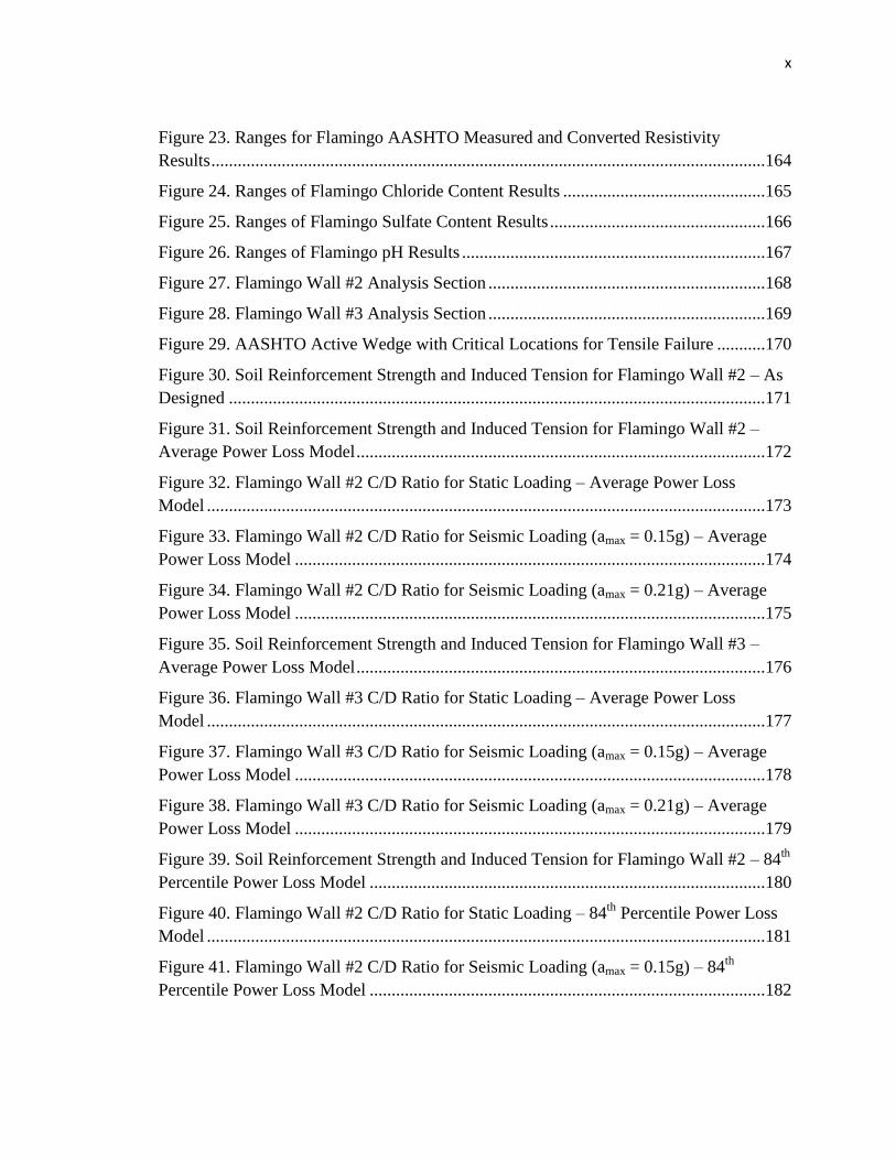
x

Figure 23. Ranges for Flamingo AASHTO Measured and Converted Resistivity

Results ..............................................................................................................................164

Figure 24. Ranges of Flamingo Chloride Content Results ..............................................165

Figure 25. Ranges of Flamingo Sulfate Content Results .................................................166

Figure 26. Ranges of Flamingo pH Results .....................................................................167

Figure 27. Flamingo Wall #2 Analysis Section ...............................................................168

Figure 28. Flamingo Wall #3 Analysis Section ...............................................................169

Figure 29. AASHTO Active Wedge with Critical Locations for Tensile Failure ...........170

Figure 30. Soil Reinforcement Strength and Induced Tension for Flamingo Wall #2 – As

Designed ..........................................................................................................................171

Figure 31. Soil Reinforcement Strength and Induced Tension for Flamingo Wall #2 –

Average Power Loss Model .............................................................................................172

Figure 32. Flamingo Wall #2 C/D Ratio for Static Loading – Average Power Loss

Model ...............................................................................................................................173

Figure 33. Flamingo Wall #2 C/D Ratio for Seismic Loading (amax = 0.15g) – Average

Power Loss Model ...........................................................................................................174


Power Loss Model ...........................................................................................................175

Figure 35. Soil Reinforcement Strength and Induced Tension for Flamingo Wall #3 –

Average Power Loss Model .............................................................................................176

Figure 36. Flamingo Wall #3 C/D Ratio for Static Loading – Average Power Loss

Model ...............................................................................................................................177


Power Loss Model ...........................................................................................................178


Power Loss Model ...........................................................................................................179

Figure 39. Soil Reinforcement Strength and Induced Tension for Flamingo Wall #2 – 84th

Percentile Power Loss Model ..........................................................................................180

Figure 40. Flamingo Wall #2 C/D Ratio for Static Loading – 84th

Percentile Power Loss

Model ...............................................................................................................................181

Figure 41. Flamingo Wall #2 C/D Ratio for Seismic Loading (amax = 0.15g) – 84th


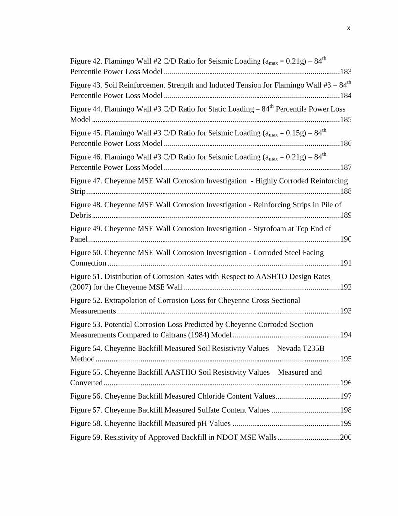
xi



Figure 43. Soil Reinforcement Strength and Induced Tension for Flamingo Wall #3 – 84th


Figure 44. Flamingo Wall #3 C/D Ratio for Static Loading – 84th

Percentile Power Loss

Model ...............................................................................................................................185





Figure 47. Cheyenne MSE Wall Corrosion Investigation - Highly Corroded Reinforcing

Strip ..................................................................................................................................188

Figure 48. Cheyenne MSE Wall Corrosion Investigation - Reinforcing Strips in Pile of

Debris ...............................................................................................................................189

Figure 49. Cheyenne MSE Wall Corrosion Investigation - Styrofoam at Top End of

Panel .................................................................................................................................190

Figure 50. Cheyenne MSE Wall Corrosion Investigation - Corroded Steel Facing

Connection .......................................................................................................................191

Figure 51. Distribution of Corrosion Rates with Respect to AASHTO Design Rates

(2007) for the Cheyenne MSE Wall ................................................................................192

Figure 52. Extrapolation of Corrosion Loss for Cheyenne Cross Sectional

Measurements ..................................................................................................................193

Figure 53. Potential Corrosion Loss Predicted by Cheyenne Corroded Section

Measurements Compared to Caltrans (1984) Model .......................................................194

Figure 54. Cheyenne Backfill Measured Soil Resistivity Values – Nevada T235B

Method .............................................................................................................................195

Figure 55. Cheyenne Backfill AASTHO Soil Resistivity Values – Measured and

Converted .........................................................................................................................196

Figure 56. Cheyenne Backfill Measured Chloride Content Values .................................197

Figure 57. Cheyenne Backfill Measured Sulfate Content Values ...................................198

Figure 58. Cheyenne Backfill Measured pH Values .......................................................199

Figure 59. Resistivity of Approved Backfill in NDOT MSE Walls ................................200

xii

Figure 60. AASHTO Resistivity Data for MSE Wall Contracts in Nevada – All

Districts ............................................................................................................................201

Figure 61. AASHTO Resistivity Data for MSE Wall Contracts in Nevada – District 1

Only..................................................................................................................................202

Figure 62. AASHTO Resistivity Data for MSE Wall Contracts in Nevada – District 2

Only..................................................................................................................................203

Figure 63. Chloride Data for MSE Wall Contracts in Nevada ........................................204

Figure 64. Sulfate Data for MSE Wall Contracts in Nevada ...........................................205

Figure 65. Power Analysis Results Identifying Minimum Statistically Significant Sample

Size ...................................................................................................................................206

Chapter One

Introduction

One of the most cost effective earth retaining structures used in transportation

applications around the United States is the mechanically stabilized earth wall system,

which are commonly referred to as MSE walls. These wall systems are comprised of a

wall facing, typically concrete, that is oriented in a near vertical to vertical direction

(Figure 1). Behind the facing there is a soil mass that has reinforcement inclusions which

stabilize the backfill soils and allow for vertical construction. Such walls are typically

found in tight intersections where room for slopes is not available. The soil

reinforcements provide tensile strength which is an ability that the soil does not have.

The spacing of the soil reinforcements, or inclusions, is relatively close together,

approximately two feet apart vertically. These soil reinforcements and their interaction

with the soil create the internal stability of the wall.

In Nevada, over 150 MSE walls have been constructed using metal

reinforcements. It is well documented that when metals are buried they can experience

corrosion due to the electrochemical interaction with the soil. This also holds true for soil

reinforcements used in MSE walls. Part of the design process involves adding extra steel

cross sectional area, also referred to as sacrificial thickness, to account for metal loss due

to corrosion. MSE backfill soils that are mild to non-corrosive only are allowed by

specifying a series of pass/fail controls (specifications) in order to limit the amount of

corrosion. Specific metal loss models have been developed from corrosion studies in

order to quantify the sacrificial thickness estimates. When the combination of sacrificial

2

thickness and mildly corrosive soils are used together, MSE walls are expected to

perform as desired.

However, if adequate sacrificial thickness is not used, or an aggressive

environment exists in the backfill there will be high rates of corrosion, which can directly

affect the internal stability of an MSE wall. At two locations in Las Vegas, Nevada,

MSE wall soil reinforcements were found to have high amounts of corrosion. These two

locations include the three MSE walls at the I-515/ Flamingo intersection and one MSE

wall at the I-15/Cheyenne intersection. The former wall reinforcement corrosion was

found by accident during construction of a soundwall at the top of one wall. The later

was also found by accident during demolition of a portion of an MSE wall for an

expansion project.

The Flamingo intersection is of significant interest because the case study is well

documented. In 2004, the reinforcements in the largest of the three walls were found to

be so corroded that the Federal Highway Administration recommended the wall be

mitigated. A cast-in-place tie-back wall was constructed in front of the existing MSE

wall. Also during that time, McMahon & Mann Consulting Engineers (MMCE) were

hired to investigate the corrosion of all three MSE walls at this intersection. Their

investigation, under the direction of Dr. Kenneth Fishman, evaluated the corrosive nature

of the backfill and collected and performed direct measurements of the soil

reinforcements for the three MSE walls. From their analysis, uniform average corrosion

loss rates were estimated. Stability analyses were also performed for the remaining two

MSE walls at the intersection based on remaining reinforcement capacity.

3

The Flamingo MSE wall investigation led NDOT to wonder how many other

MSE walls may be experiencing stability issues due to high rates of corrosion. The

research presented in this report is focused on developing a systematic approach to

answer this question. There are other MSE wall case studies that can be used to help in

this research, such as the South African MSE wall case study and the Caltrans Mariposa

MSE wall case study. However, the data collected by MMCE presents a detailed MSE

wall evaluation within Nevada. While MMCE focused on a uniform corrosion loss

evaluation, further analysis, which focuses on a statistical evaluation of loss

measurements to predict future stability issues due to corrosion loss, is presented in this

report. The two remaining unmitigated walls at Flamingo are the focus of the stability

analysis because they have not been mitigated and possess the ability to cause disruption

to the transportation corridor and potential loss of life if they fail. A statistical approach

has also been used to evaluate the characteristics of the backfill sampled in 2005 from

behind the MSE walls and make comparisons to the data from approved backfill sources

prior to construction in 1985.

The results from the statistical analyses performed provide the framework to

select other walls that may be experiencing similar rates of corrosion. A database of

existing MSE walls has been developed in order to aide in the selection of suspect walls.

Wall locations and characteristics of the walls at those locations have been collected and

included in the database. From this database, walls can be ranked in order of perceived

severity so that future MSE wall evaluations can be performed. Specific methods for

future analysis have also been developed and presented in this report as well.

4

1.1 Project Information

This research is a result of previous investigations and measurements produced by

several groups including Nevada Department of Transportation (NDOT) and McMahon

& Mann Consulting Engineers at the three MSE walls located at the I-515/Flamingo

Road intersection in Las Vegas, Nevada. A proposal for further investigation into the

severity of corrosion of MSE wall reinforcements was proposed by Drs. Raj Siddharthan

and Barbara Luke from the University of Nevada in Reno and Las Vegas, respectively.

The scope of the proposal is outlined below. The research and results presented in this

report use this scope as a framework to identify potential corrosion problems, quantify

these problems, and make predictions about their potential to affect other MSE walls in

Nevada.

1.1.1 Scope of Project

To identify the extent of the elevated levels of corrosion for walls across Nevada,

a series of six tasks were defined in the proposal to NDOT. These tasks are as follows:

1. Develop an Inventory of NDOT MSE Walls and Literature Survey;

2. Synthesize Available Field Inspection Database on the Behavior of Nevada MSE

Walls;

3. Review the Report Relative to the Flamingo MSE Walls Prepared by McMahon

& Mann, Consulting Engineers;

5

4. Assemble Data on MSE Wall Corrosion Performance and Specifications from

Other States;

5. Identify and Synthesize Data on Important Factors that Affect Corrosion of

Nevada MSE Walls; and

6. Select Candidate Sites for Phase II Investigation.

1.2 Organization of the Report

This report is divided into seven chapters where the introduction and conclusions

and recommendations are the first and last chapters. In Chapter 2 there is a thorough

discussion of the history of MSE wall corrosion background. This background starts with

a development of historical buried metal corrosion studies relevant to MSE walls. There

are several important MSE wall case histories that are summarized because of their

relevance. This chapter also gives historical background regarding the agencies that have

developed specification guidelines for corrosion issues related to soil reinforcements in

MSE walls. Chapter 3 focuses on the mechanisms of corrosion of buried metals and

discusses the testing issues and methods used to identify corrosive backfills. In this

chapter an important development of the correlation between the Nevada T325B and

AASHTO T-288 soil resistivity test methods is developed.

In Chapter 4 two crucial MSE wall corrosion case studies that have been

conducted in Nevada are discussed. These two case studies include MSE walls at the I-

515/Flamingo intersection and the I-15/Cheyenne intersection. Statistical analysis of the

6

reinforcement section loss due to corrosion is performed. Statistical analysis of the

differences in electrochemical properties measured in the backfill approval process

compared to the in-place sample properties is also presented. Wall stability analyses are

conducted for two Flamingo MSE walls as well.

Chapter 5 and 6 include proactive discussion of other MSE walls in Nevada that

may be experiencing corrosion. Chapter 5 focuses on a database of the NDOT MSE

walls and their characteristics. Chapter 6 is a detailed discussion of which NDOT MSE

walls should be investigated further. A suggested evaluation sequence and statistical

sampling practice is also introduced.

The conclusions of the report and recommendations for Phase II work are

included in Chapter 7. Recommendations for modification to current NDOT practices

with respect to MSE wall corrosion are also discussed. The tables and figures referred to

throughout the report are included after the text. The references follow the figures.

There is an appendix (Appendix A) at the end of the report. In this appendix, sample

calculations for the MSE wall stability analysis are included.

7

Chapter Two

Historical Background

In order to better understand the issues related to corrosion of MSE walls a

summary of some historical background has been included in this chapter. Corrosion

studies have been conducted on metals buried in soil. These represent the basis for the

estimation of sacrificial steel thickness that needs to be added in order to account for the

natural phenomenon of corrosion. While the inclusion of sacrificial steel has been

successful with a number of walls located around the globe there are a number of walls

that have been found to perform poorly. A summary of some of these walls has been

included to highlight some of the issues that still remain. In recent years, because of the

unknowns that still surround corrosion of MSE walls, surveys of MSE wall owners,

typically state DOTs, have been conducted. Three of these surveys, which represent the

most recent surveys, give an overall idea of the number of MSE walls that exist in the

United States and some of the findings of walls that have faced corrosion issues. Finally,

this chapter also identifies the specific historical recommendations and practices by

FHWA, AASHTO, and Nevada.

2.1 Historical Corrosion Studies

While there has been a number of corrosion studies of metals buried in soil, there

are two that stand out for MSE wall corrosion issues. These are the forty-five year study

performed by the National Bureau of Standards and a study performed by a French

laboratory in conjunction with the Reinforced Earth Company. The first is a general

study of an assortment of metals in a variety of soil types and environmental conditions.

8

The latter is more specific to MSE walls focusing on soils and conditions that are more

representative of MSE wall construction practices.

2.1.1 National Bureau of Standards Circular 579

In April 1957 the National Bureau of Standards (NBS, now the National Institute

of Standards and Technology) released its NBS Circular 579 (Romanoff 1989). This

circular was the result of a forty-five year study (commissioned in 1910) of underground

corrosion of metals in different environments which is considered by many as the

beginning of concentrated research on the effects different soil conditions on the

corrosion of metals. One of the outcomes of this research is an understanding that pH,

soil resistivity, and soluble salts, in conjunction with moisture content, affect the rate at

which corrosion occurs. From this understanding engineers are able to estimate metal

loss of buried metal structures, such as pipelines and, more important to this paper, the

metal loss of soil reinforcements for MSE walls.

From this extensive study several concepts of the corrosive nature of soil became

apparent. The development of the empirical relationship of time and metal loss

(measured by pitting depth) is expressed as,

P=ktn (2.1)

where P is the pit depth at time t, and k and n are constants that depend on the soil and

metal characteristics, respectively. It was typically seen that the corrosion rate was

higher at original burial and tended to tapper off to a lower rate as time since burial

9

continued. Much of the current practice in metal loss assumption stems from this study.

However, it was widely understood that soils which were used in these tests were not

entirely representative of the soils used in the typical construction of MSE walls.

Specifically there were only a few sites where sands and gravels with low fines content

and low plasticity were tested. Further studies were subsequently conducted in order that

the constants in Equation 2.1 could be more representative of the backfill materials used

in MSE wall construction.

2.1.2 Reinforced Earth Company Study

The Reinforced Earth Company along with the Laboratorie Central des Ponts et

Chaussees (LCPC) and Terre Armee International realized the limitations of the NBS

study with respect to MSE wall corrosion (Darbin et al. 1988). In 1974 these two groups

combined efforts to study the effects of MSE backfill on soil reinforcements, more

specifically buried galvanized and bare steel reinforcements. The reinforcements were

tested in controlled soil boxes containing a variety of soil types with differing

electrochemical characteristics. Also included in this study was the evaluation metal loss

of in-service soil reinforcements of forty existing Reinforced Earth Company walls

located in France.

The environmental controls of some of the tests included five soil types and a

variety of water contents. Electrochemical effects of chlorides and sulfates were

evaluated using one soil type and various levels of the soluble salts along with varying

10

water contents. The reinforcements used in the tests included black steel (not galvanized)

and steel that was galvanized, but with different thicknesses of zinc coatings.

In order to evaluate the metal loss of the samples due to corrosion two methods

were used, which included container tests and electrochemical tests. With the container

tests samples were accurately weighed, buried and exhumed at specific time intervals and

then cleaned and weighed again. The difference in weight was then converted to a

uniform metal loss. The samples that were measured electrochemically using

polarization resistance measurements were then compared to the container tests, which

showed that in most cases both predicted similar uniform metal loss rates. Although

much of the data revolves around uniform loss, the authors pointed out that once the

galvanized coating had been oxidized the underlying steel became pitted and it was

confined to localized regions (Darbin et al. 1988).

After a ten year study of these buried reinforcements, conclusions were drawn as

to the applicability of the NBS data and new design methods especially concerning

buried steel with galvanized coatings. It was found that water content, sulfates and

chlorides all played significant roles in the rate of corrosion of steel reinforcements

within MSE backfill. More precise values for the constants for input into Equation 2.1

were also developed from the ten years of data based on the “practice to restrict

extrapolations to a period lasting no more than ten times the duration of the actual

measurements” on a logarithmic scale (Darbin et al. 1988, pg. 1031).

11

2.2 Historical Field Investigations

One of the primary and effective methods for learning about corrosion and its

effects on soil reinforcements is to conduct field investigations of existing MSE walls.

These types of investigations are very costly and in transportation corridors cause extra

burden on the population that depend on their usefulness. With that in mind it is

important to review case studies and investigations that others have performed so that

lessons can be learned. The following case studies highlight some of the many studies

that have been performed in the United States, as well as other countries.

2.2.1 Caltrans 14 Wall Study

The California Department of Transportation (Caltrans) undertook a survey and

investigation of fourteen Mechanically Stabilized Embankments located across the state

(Jackura et al. 1987). Since 1979 Caltrans has implemented the practice of installing

non-stressed rods or coupons into the MSE backfill. These rods are removed and

inspected at specific time intervals and the corrosion loss is measured and compared to

the design assumptions. In 1985 Caltrans removed and inspected the sample coupons

from a wall located in Mariposa County. There was severe pitting corrosion on the

samples, which were only six years old. From these observations Caltrans decided to

investigate the Mariposa wall site as well as thirteen other wall sites.

Although the Mariposa County wall experienced higher than expected corrosion,

the other thirteen walls in the investigation were observed to have lower rates than the

designed corrosion rates. The Mariposa wall was constructed with plain steel

12

reinforcements that did not have a galvanized coating. However, three other walls also

were constructed with plain steel reinforcements, but exhibited a more uniform corrosion

and the loss rate was lower than the design rate assumed by Caltrans. The Mariposa wall

experienced pitting corrosion and even when the pitted areas were excluded, the uniform

loss was 167% of the Caltrans design values. It appeared that the galvanized

reinforcements had good coverage and were performing in an acceptable manner.

Caltrans’ summary of other walls states that those with galvanized coatings did not have

very many locations where the base steel had been exposed. It is interesting to note that

the walls that were investigated were between three and fourteen years old. The current

AASHTO design assumption (AASHTO 2007) is that the galvanized coating should last

at least sixteen years. Therefore, it should not be a surprise that the younger walls did not

have exposed base steel.

During the investigation Caltrans noted that there were differences in soil density

between soils near the facing of the walls and soils found further from the wall facing.

They noticed that there appeared to be a looser area within three feet of the facing while

becoming increasingly dense as samples were retrieved farther from the facing. This is

most likely due to constructions practices, including using lower compactive efforts near

the first three feet from the facing. This practice proved to create an environment that

was conducive to corrosion because of aeration differentials near the face and further

back into the reinforce soil. More on this phenomenon can be found in Chapter 3. The

other issue that was noticed at the Mariposa site was that the backfill consisted of a rocky

fill and cohesive fines which differs from backfill that is commonly used. There is a

13

similarity here to the next MSE wall that had a poor performance history located in South

Africa.

2.2.2 South African Wall Study

At the Tweepad mining operation in South Africa, a series of Reinforced Earth

Company walls were constructed in 1978 and 1979 at heights of up to 41 meters to

support a gravity separation plant (Blight and Dane 1989). In 1980, there was a failure of

a MSE wall at another mine in South Africa because of corrosion of the steel reinforcing

strips in the backfill. As a result of this failure, the Tweepad mine became interested in

the potential for corrosion of the soil reinforcements of their MSE walls. The

investigation that resulted found that the metal strips had experienced corrosion in the

form of severe pitting. Over the next several years the wall performance was monitored.

The monitoring included strip tension measurements and outward deformation

measurements. All of the walls at the complex showed deformation by rotation about the

base without much translation. Eight years after construction the walls were removed

and new MSE walls were constructed in their place.

The original construction practices, design methods and backfill materials were

then evaluated because the shorter service life of eight years or 26% of the original thirty

year design life posed a serious concern. During the design phase the electrochemical

requirements of the backfill material were relaxed because the mine only needed a thirty

year design as opposed to the seventy year design that typically accompanies the more

stringent electrochemical requirements. The ancient beach sand containing high salt

14

content was used for the backfill and it was compacted using sea water, which introduced

more soluble salts, as well. Despite these corrosion concerns, galvanized strips with one

millimeter of sacrificial steel were used and thought to be sufficient for the thirty year

design life.

The Tweepad MSE wall investigation concluded that the most significant

mechanism of corrosion was differential aeration. The cause of the differential aeration

was the inclusion of clay lumps in the backfill. In areas where the clay lumps were in

contact with the soil reinforcing strips pitting developed. As will be discussed in Chapter

3, differential aeration is caused by varying oxygen levels along the surface of the steel

causing regions where differential oxygen levels occur to become anodic, which can

result in localized pitting.

There were several lessons learned from this wall study. The reconstruction of

these walls included a more controlled gradation of backfill with a limited amount of

fines passing the 75 μm sieve in order to eliminate the prominence of clay lumps. Limits

on electrochemical properties of the backfill, including the use of fresh water instead of

sea water, were recommended for durability. With these modifications in the design and

construction it is believed that the new walls will survive the design life required for

mining operations.

2.2.3 Flamingo Wall Study

As discussed in the previous chapter, a series of three MSE walls at the

intersection of I-515 and Flamingo Road in Las Vegas, Nevada is the starting point of the

15

research presented in this report. In 2004, after approximately twenty years of service

life, a contractor of Nevada Department of Transportation (NDOT) was excavating at the

top of one of these MSE walls for the construction of new sound walls along I-515.

During the process of the excavation some of the upper layer steel reinforcements were

accidentally penetrated. The reinforcements that were visible appeared to be highly

corroded, to the point that NDOT halted work on the sound walls and began a

reinforcement corrosion investigation.

With the assistance and advisement of the Federal Highway Administration

(FHWA), NDOT excavated several test pits at the top of the tallest wall. Soil and steel

samples were collected and electrochemical tests were conducted on the soil. The results

of the electrochemical tests, including soil resistivity, pH, sulfates and chlorides, showed

that the backfill soils had significantly higher than recommended levels of sulfates. The

soil resistivity was found to be significantly lower than the backfill that was approved

during construction in 1985. The steel reinforcements in the MSE wall backfill were

highly corroded with some of the steel bars having only pencil tip thick cross sections

remaining. McMahon & Mann Consulting Engineers were asked to perform a more

thorough and detailed investigation into the corrosion of these three walls. More test pits

were advanced into the upper surfaces of these walls, samples were exhumed and

measurements of the diameter of the remaining steel were taken at hundreds of locations.

Backfill soils were also sampled and laboratory measurements including index testing

and electrochemical testing was performed.

16

Some of the results of this investigation show that these three walls have

experienced corrosion at a significantly higher rate than was anticipated during design.

The wall was constructed using black or uncoated steel welded wire grids, which is not

common in MSE wall construction. These steel reinforcements experienced significant

pitting corrosion and it was noticed that the reinforcements located in the differential

compaction zone directly behind the facing had developed pitting corrosion, likely due to

differential aeration through the development of macro cells. The backfill soils consisted

of generally silty gravels and as previously stated had high sulfate contents and low

resistivity. The tallest wall, thirty-two feet at its highest point, was retrofitted with a tie-

back wall because it was decided that the wall had experienced such a high amount of

corrosion that it was no longer an effective retaining structure. The other two walls

remain in place due to their lower heights. More on the analysis of this study and the

measurements that were performed can be found in Chapter 4.

2.3 Soil Reinforcement Corrosion Surveys

There are three recent corrosion surveys detailed here. These surveys are aimed

at collecting data on MSE walls across the United States and internationally. One of the

underlying aims of each of these surveys is to obtain a better understanding of MSE wall

behavior with respect to soil reinforcement corrosion. Because of the existence of these

three surveys there was no necessity to develop another survey, since it would be similar

to the three surveys detailed below.

17

2.3.1 AMSE Survey

In 2006, the Association of Metallically Stabilized Earth (AMSE) published a

series of recommendations for AASHTO to consider with regards to corrosion of steel

reinforcements in soil (AMSE 2006). Included in this publication was a request for

AASHTO to consider reducing the corrosion rates used to calculate the amount of

sacrificial steel required for the design of MSE walls. Using research and a survey of

walls located in the United States and internationally, AMSE detailed its concerns

regarding what it saw as the overly conservative current AASHTO guidelines. One of

the main contentions raised in this 2006 paper is that, in general, MSE walls with

galvanized steel reinforcements have behaved very well over the past thirty years (the

typical design life is seventy-five years). There have been a few specific sites that have

performed poorly, but there are issues that were found at each of these sites that do not fit

within the normal trend of data across the United States.

A substantial number of investigations were cited by this 2006 paper that have

been performed by state DOTs, other agencies, and member companies of AMSE. These

results support the idea that many of the walls that have undergone investigations show

corrosion rates equal to or less than the AASHTO guidelines require for design and

construction.

When closely looking at the survey data, some very interesting observations can

be made. The survey includes a catalogue of 780 MSE walls randomly sampled from the

approximately 40,000 walls that have been constructed since the early 1970’s in the

18

United States. Almost half of the walls in the database are located in the western United

States, and it should be noted that this database may only be representative of walls that

have been constructed prior to 1990. From the survey data it can be seen that galvanized

strip reinforcements were more commonly used throughout the United States, with the

exception of the western states where galvanized welded wire mesh and barmat type

reinforcements are more common.

As has been emphasized in previous discussions, the backfill material is the most

significant factor in the corrosion issue. Of the thirty-eight states that provided 253

backfill records, there were 194, 133, and 130 records of measurements of resistivity,

chlorides and sulfates, respectively. A large majority of the wall data that is presented

shows soil resistivity data of greater than 10,000 ohm-cm, which is considered non-

corrosive. As will be mentioned in Chapter 3, there is a relationship between resistivity

and chlorides and sulfates (Figure 2, Elias 1990). However, it is commonly seen that

resistivity is a useful overall predictor of corrosion resulting from salt content, including

chlorides and sulfates.

Of the 780 walls in the AMSE catalog there are eleven wall locations that have

been specified as poorly performing. This may seem like a small percentage, but high

corrosion rates found in at least one of these wall locations (Nevada Flamingo Walls) was

only discovered by accident during excavation of a soundwall footing above the MSE

wall. It should also be noted that the resistivity of this backfill was assumed to be greater

than 3,000 ohm-cm until electrochemical tests were performed subsequently. This is

interesting because the survey results lead one to believe that only thirteen walls have soil

19

resistivity at or below the 3,000 ohm-cm range. This may not be an entirely accurate

representation of backfill characteristics, as will be discussed in Chapter 3, 4, and 6. It

should be noted that there are very few walls in the United States that have been

investigated with the use of physical measuring of cross sectional area loss.

Also, the pH appears to be within the ranges where, by definition, acidic or

alkaline conditions do not exist (Figure 3). There are many references that suggest that

pH is not a good measure of soil aggressiveness (Zhang 1996) as much of the time the pH

falls between the accepted range of 5 to 10 for backfill soils. With the limitations in

corrosion prediction using pH and a good portion of data falling within generally

accepted values, minimal importance will be placed on pH data later in this paper.

One of the final issues that is presented by this survey is that of monitoring

practices. From the survey results it appears that walls constructed between 1970 and

1980 are the ones most commonly monitored for metal loss. The southeastern U.S. far

surpasses other regions in regards to conducting these monitoring practices. The metal

loss monitoring practices are typically of the non-destructive type, such as polarization

resistance and half-cell potential measurements.

2.3.2 NCHRP Survey

One of the more recent publications presenting data and information about

corrosion practices and issues (for MSE walls, soil nail walls, and soil and rock anchors)

in the United States is a National Cooperative Highway Research Program (NCHRP)

project conducted for the Transportation Research Board and identified as NCHRP 24-28

20

(2007). An interim report presenting the findings of Phase 1 in a multiphase project

included a ten question survey that was sent to all fifty States and Washington D.C.

Thirty-two replies were received and several with additional comments to the initial

survey. This survey was also sent to several jurisdictions in Canada, where seven of

seven jurisdictions replied to the survey. One of the purposes of the survey was to

identify the number and ages of metallic earth reinforcements located in each jurisdiction.

Also addressed in the survey are questions regarding accelerated corrosion issues and

corrosion monitoring practices. The survey concludes with questions about the potential

willingness to share information and plans for wall demolition and reconstruction.

The specific data that has been collected in the survey portion of the project has

been focused on inventory quantification. There are a couple of important conclusions

that can be made from this survey. There are a large number of states that have dozens to

hundreds of MSE walls. There are also a number of states that are willing to share their

data with the NCHRP project.

The interim report also includes information regarding the specific findings of

several studies that have been conducted on MSE walls. One of the more interesting

summaries of information is located in a table discussing MSE wall locations that have

detailed data. This table has been reproduced as Table 1. There are seven states that

have been included in the table. There is a rating of backfill conditions that range from

poor to good.

21

Four of the seven states have backfill conditions that have a portion in the

poor region of the range.

Three of the four of these states, including California and Nevada, also

have direct physical measurements that have been collected.

None of the states with good ratings have any direct physical

measurements.

This may be an important issue because as discussed with walls such as those found at

the Flamingo site in Nevada, the outward appearance is not an indicator of a distressed

condition. However, the Flamingo walls had undergone significant corrosion at higher

rates than were anticipated.

2.3.3 Oregon Department of Transportation

In a research study, published in May 2008, performed by Oregon State

University for Oregon Department of Transportation a survey of states and their MSE

wall practices was presented (Raeburn et al. 2008). The questions of the survey revolve

around the goal of obtaining information regarding the practices of other states with

respect to materials used in MSE walls and corrosion issues. Altogether it consists of

nine questions that focused on metallic soil reinforcement use, poor performance, and

corrosion. There are not many quantitative results from this survey, which suggests that

state DOTs do not really feel there is a problem with their MSE walls with respect to

corrosion. The supporting evidence is that five of the eight responding DOTs said that

22

they have not taken any measurements of corrosion rates on their walls. As has been

seen in other MSE walls, without investigations into corrosion rates, either through

thoughtful investigation (Caltrans Mariposa wall) or by accident (NDOT Flamingo walls)

one cannot be sure that corrosion issues do not exist without proper monitoring of

existing MSE walls. If state DOTs do not make observations to compare measured

corrosion rates to the rates used in the design process, they could be in a similar situation

to Nevada DOT who did not know of corrosion issues until accidental discovery. This

can be a very costly method of corrosion monitoring.

One other conclusion that can be drawn is the significance of the use of steel

reinforcements in the construction of MSE walls. Of the seven respondents, four states

reported that 80% to 100% of their MSE walls were constructed with steel

reinforcements in the past five years, including Nevada reporting 100%. This is

significant because it has only recently been an accepted option for DOTs to construct

MSE walls with materials other than steel, such as geosynthetic reinforcement which

have different corrosion resistance characteristics. Five of seven respondents report that

at least 80% of their entire MSE wall inventory consists of walls constructed with

metallic soil reinforcements.

2.4 Soil Reinforcement Corrosion Recommendations and Practices

The information in this section is meant to provide a historical background for the

development of today’s corrosion standards and specifications. While this section reports

on the limitations on soil properties, these values can vary greatly depending on which

23

test method is used to measure these properties. Although AASHTO has specified

certain test methods, many state DOTs have also selected their own test methods. Each

of the test methods will not necessarily produce similar results. More discussion of these

test methods and their potential for variation is included in Chapter 3. The information

below is only meant to provide a context for how the specifications have evolved over

time. These historical changes are related to laboratory corrosion testing and observation

of existing structures and their performance. While some of the changes in the

specifications over time can be linked to testing method and observation, some of the

changes appear to be more related to the fact that corrosion in MSE wall inclusions is still

not as well understood as engineers would like since the cost of destructive testing and

mitigation is high, a conservative solution of providing sacrificial steel has become the

preferred design approach.

2.4.1 Early Years

Many of the corrosion recommendations from the early years of steel

reinforcement use were the result of field tests and observations from studies such as the

NBS forty-five year tests and the French laboratory studies, as well as observations from

buried pipe groups. The concept of an addition of sacrificial thickness, which was

pioneered by the Reinforced Earth Company, was based on an assumed metal loss rate

for the design life of the structure. In 1978 the French Ministry of Transport had

electrochemical backfill requirements of a pH range of 5-10, a minimum soil resistivity

of 1,000 ohm-cm, a maximum chloride content of 200 parts per million (ppm) and a

maximum sulfate content of 1,000 ppm (Blight and Dane 1989).

24

Prior to this there are very limited quantifiable requirements that have been

recommended. As will be seen below it was not until the 1990s that the American

Association of State Highway and Transportation Officials (AASHTO) included any

requirements into their Standard Specifications for Highway Bridges. It is interesting to

note that a majority of the walls included in the AMSE survey (discussed earlier) were

constructed prior to the incorporation of corrosion loss rates in AASHTO design. This is

not to say that designers did not include sacrificial steel in their wall designs. However,

these walls may have been constructed with more aggressive backfill or less sacrificial

steel, or both.

2.4.2 FHWA

For more than twenty years the Federal Highway Administration (FHWA) has

published guides and resources to assist engineers in the design of MSE walls. There are

two publications that will be the focus of this historical background (Elias 1990). The

first, FHWA-RD-89-86, published in 1990, presented a very thorough set of guidelines

and theory of corrosion of steel and geosynthetic reinforcements buried in soil. This

publication included the French and German study data, NBS Circular 579 corrosion

concepts, as well as data and standards collected from other agencies, both internationally

and in the United States.

One of the main objectives of the 1990 FHWA publication is to provide

background theory and information regarding the current understanding with respect to

corrosion issues specifically for MSE walls. Soil backfill electrochemical topics are

25

discussed and there is a significant detailing of the tests and their strengths and

weaknesses at measuring the important electrochemical properties. The corrosion

mechanisms that result because of soil aggressiveness are also summarized. With the

development of the background thoughts and current considerations FHWA presented

corrosion rates that it felt were properly conservative to address both pitting and galvanic

corrosion. More on these two types of corrosion are included in Chapter 3. It appears

that AASHTO drew their first corrosion recommendations from this document.

In 2000, FHWA published a follow-up report that also addressed corrosion of

MSE soil reinforcements, and both metal and geosynthetic reinforcements were included

again (Elias 2000). This document is very similar to the previous version with respect to

metal corrosion issues. Some of the modifications made in this version are more

readable; however, some important information regarding test methods was excluded.

Both of these publications prove to be very valuable reading for metal corrosion

background information. Much of the reasoning behind the current thoughts on corrosion

rates and metal loss design considerations is presented in these publications. The strong

point of the 1990 publication is that it discusses a variety of test methods that can be used

to evaluate the electrochemical characteristics for backfill materials. However, the

current practice tends to incorporate the test methods discussed in the 2000 version,

making the 1990 version useful only as a historical context of some past practices.

26

2.4.3 AASHTO

The literature review of the AASHTO Standard Specifications for Highway

Bridges began with the review of the eleventh edition (AASHTO 1973) because NDOT

constructed its first MSE wall in Lovelock, Nevada in 1974. With a thorough review of

the eleventh edition it was found that there was no reference to the design of MSE walls

(or Reinforced Earth walls, as they were known at the time) in the Division 1 section and

there was also no mention of corrosion or backfill properties in the Division 2, or

construction section of the edition. It is worth noting that there is very little information

about any retaining walls in this edition. This holds true through the fourteenth edition

(AASHTO 1989).

In 1992 the fifteenth edition was released. With its release was a watershed of

design specifications and requirements for retaining walls in general. More specifically,

it is the first time that MSE type walls are mentioned. This is likely the result of the

above mentioned 1990 FHWA publication (Elias 1990). Included in Division 1 design

section are design life requirements of seventy-five years and 100 years for permanent

and critical structures, respectively. The concept of sacrificial thickness was also

included and standard corrosion loss rates were specified. In Division 2, the construction

division, gradation and electrochemical limits are placed on the backfill materials used in

construction of MSE walls. Although, it is important to note that there are no

specifications regarding which test procedures should be used to verify the

electrochemical limits of the backfill (AASHTO 1992). The AASHTO electrochemical

27

specifications are presented in Table 2 in a timeline fashion including the NDOT

specifications to show their relationship over time.

The sixteenth edition was presented in 1996. In this edition the specifications for

standard corrosion rates and electrochemical properties were modified, but again did not

specify the test procedures to use to verify these properties (AASHTO 1996). There were

some other changes in the corrosion issues related the MSE walls in the seventeenth

edition (AASHTO 2002). The electrochemical requirements were moved into the design

section (Division 1), but more importantly the test procedures were specified as

AASHTO testing procedures. Along with this inclusion there is more discussion with

respect to corrosion including the following statement. “These sacrificial thicknesses

account for the potential pitting mechanisms and much of the uncertainty due to data

scatter, and are considered to be maximum anticipated losses for soils which are defined

as nonaggressive” (AASHTO 2002 pg.152). Up until this edition, the epoxy coating of

steel was included as an option. However, there is a note that states that there is no

sufficient data to support the practice of epoxy coating the soil reinforcements. The most

recent AASHTO publication is the LRFD Bridge Design Specifications (AASHTO

2007). Other than the significant change from ASD design methods to LRFD design

methods the information regarding electrochemical testing and accountability of

corrosion through the addition of sacrificial steel remains the same as the 17th

edition.

28

2.4.4 Nevada Department of Transportation

A review of the Nevada Department of Transportation Standard Specifications for

Road and Bridge Construction (also referred to as the Silver Book) gives a historical

context for corrosion specifications in Nevada. Using the 1968 Specifications as a

starting point there were no references to corrosion of MSE walls or MSE walls in

general until the 1986 Silver Book. Between the 1976 and 1986 versions of the Standard

Specifications there was at least one set of interim provisions. However, these

memorandums were not readily available. The only records for these electrochemical

corrosion requirements for backfill soils were found on the laboratory testing records of

backfills that the contractor submitted for acceptance testing prior to use. One example

of this can be found in the MSE backfill test data for Contract 1918. This set of

electrochemical specifications is included in Table 2. More on the approval practices is

discussed later in this section.

In the 1986 Silver Book there are several limiting characteristics of soils to be

used in MSE wall backfill. These are presented in tabular form in a timeline relationship

with AASHTO specifications (Table 2). The pH has an acceptable range between five

and ten while the measured soil resistivity had a minimum limit of 3,000 ohm-cm. Both

the chlorides and sulfates were bounded by maximum allowable values of 200 and 1,000

parts per million (ppm), respectively. These values compare well with the French

Ministry of Transport limitations except for the resistivity minimum value which was

increased from 1,000 to 3,000 ohm-cm. As discussed earlier, it was not until the 15th

edition in 1992 that AASHTO published electrochemical specifications for MSE backfill.

29

The next Silver Book that was published was in 1996. In this publication, as with

the 1996 AASHTO specifications the electrochemical specifications were modified to

what they are today. Both the pH and resistivity remained the same when compared to

the 1986 Silver Book. The permitted salt content was reduced for chlorides from 200 to

100 ppm while the sulfates were reduced significantly from 1,000 to 200 ppm. Similar

guidelines have been presented by FHWA in their 1990 Task Force 27 recommendations,

1990 corrosion guidelines (Elias 1990) and the 2000 FHWA corrosion guidelines (Elias

2000). These electrochemical specifications are also the same as those found in both the

current NDOT Silver Book (2001) and AASHTO specifications (2007 LRFD with 2008

Interim).

With the exception of one or two recent walls, the practice of acceptance testing

prior to backfill use by the contractor has been the main method for measuring the

electrochemical properties. The contractor will submit samples, NDOT personnel will

test the soils and either approve the source or deny the specific source until further testing

proves the source is acceptable. This will occur prior to the construction of the MSE

walls. It should be noted that a review of the approved and rejected sources shows that in

many instances a single source will provide backfill soil samples that are within and

outside the specifications, but once the source provides material passes, that source is

approved. There are a variety of questionable issues that are present in this practice.

These will be discussed in detail in Chapter 4 and 6.

As previously mentioned, there are a handful of walls that have a different set of

methods for the acceptance of MSE backfill. Several recent NDOT wall construction

30

specifications (production testing) have required (e.g., I-15 North Design Built Project in

Las Vegas) that the contractor stockpile a certain amount of potential backfill material on

the jobsite prior to construction of the MSE walls. The acceptance test samples are taken

directly from these jobsite stockpiles and then tested by NDOT personnel. If the material

is accepted then it is used for construction. However, if the jobsite stockpile is rejected

that stockpile cannot be used as MSE backfill. This provides a more controlled

atmosphere where soils that are to be used are more representatively sampled and tested.

2.4.5 Local States

The literature review in this research included the review of the current MSE

backfill corrosion practices for other western states surrounding Nevada including

California, Oregon, Utah and Arizona. Western states have been the focus of this section

because they are most likely to represent similar challenges with aggressive arid desert

soils that are found in Nevada. Table 3 presents the electrochemical specifications for

each of these states. When found, a test method is also specified for each electrochemical

backfill property. This is a critical piece of information because of the wide variety of

test methods used and the range of values that can be produced by each test for the same

test sample. In many instances the chloride and salt content tests are not evaluated if the

resistivity is a minimum of 5,000 ohm-cm. This is due to the thought that these soils will

not likely have large salt contents and the soils can be classified as mildly corrosive

(FHWA 2000). Specifications for states that have not been included in this table can be

found on the FHWA state specification information clearinghouse

(http://fhwapap04.fhwa.dot.gov/nhswp/index.jsp).

http://fhwapap04.fhwa.dot.gov/nhswp/index.jsp

31

Along with the importance of soil aggressiveness is the type of steel

reinforcement used. All of the states included in Table 3 have specified that the steel

inclusions should be galvanized per ASTM A-123. This is an aim to insure that the

corrosion rate will be similar or less than that of the specified rate loss of metals provided

in the current AASHTO design guidelines.

32

Chapter Three

Corrosion Background

3.1 Corrosion of Buried Steel

Corrosion of metal reinforcements in soil is a natural phenomenon where the

metal attempts to return to its fundamental state. Typical metals, like galvanized steel

reinforcements, corrode back to a more stable state of salts and oxides when left alone in

soil. It is important to have an understanding of the mechanisms of corrosion of steel in

soil. With this understanding potentially problematic situations can be reduced or

avoided altogether. Corrosion mechanisms require an environment that is conducive to

electron transfer. One way to deal with this issue effectively is to control the

environment in such a way that electron transfer is made more difficult. It has been

found that there are certain variables that can estimate the ability of the soil to hinder

electron transfer. These variables include soil resistivity, soluble salt content and pH.

With limits placed on these variables of backfill soils, corrosion rates can be estimated

and taken into account by way of additional steel and/or galvanization for a non-

structural sacrificial coating. The following sections discuss the corrosion mechanisms,

predictive measures and expected corrosion rates.

3.1.1 Corrosion Mechanisms

The corrosion mechanism for steel and other ferrous metals is typically

electrochemical in nature. Electron flow from the anodic portion of the metal surface to

cathodic portion is dependent on the existence of an electrolyte surrounding the metal

inclusion in the soil. This exchange can typically occur at two levels, commonly referred

33

to as micro and macro cells. While there are a variety of forms of these two types of

corrosion, only two will be discussed here because of their significant effect on the

corrosion experienced by MSE walls in typical backfill environments. These two

corrosion types include pitting corrosion and galvanic corrosion for micro and macro cell

corrosion mechanisms, respectively.

In the case of micro cells or localized corrosion, pitting corrosion is most

commonly discussed in the literature, based on observations during site investigations

and laboratory testing. Pitting corrosion occurs in areas on the metal surface where there

are micro irregularities. These surface irregularities can create an electrolytic cell where

an anode and cathode are developed. The area required for an anode is typically very

small while the cathodic region is significantly larger. This cell can create a very large

electrical potential that allows electron flow at an increased rate compared to the

surrounding surface area. With this higher rate of exchange of metal ions from the anode

to the cathode, significant metal loss can result. These areas are commonly referred to as

pitted regions on the surface of the metal. These pitted areas are described as deep or

shallow, where the deep regions produce deep cavities of metal loss over a small area and

the shallow pits affect larger areas but are not as deep (ASM International 1987).

Differential pH levels are created within the pit that, with an effective electrolyte, will

allow the metal ions to leave the surface on the anode side of the metal and then be

deposited on the cathode side of the electrolytic cell. Soil saturation plays an important

role in the creation of an electrolyte. Without proper levels of saturation an effective

electrolyte is not developed. In the French laboratory tests in the 1970s it was found that

34

saturation ranges of 30% to 50% produced the highest potential for corrosion to occur

(Darbin et al. 1988). In the case of the Flamingo walls the saturation levels were

estimated as ranging from 25% to 40% (Fishman 2005). Many MSE walls will likely

have an optimal amount of saturation because of the use of water to compact the soil,

which is locked into place. There are seasonal variations in moisture content that can

make electrolytic cells stronger during certain times of the year. The process of pitting

corrosion is a self-sustaining process that can result in significant metal loss compared to

situations where uniform metal loss occurs (ASM International 1987). Several studies,

such as the NBS forty-five year experiment, have shown that pitting can occur at three to

five times the rate of uniform metal loss (Romanoff 1989). While there is always a

possibility that metals buried in soils can experience pitting corrosion, there are methods

to reduce the likelihood or severity. The most common methods used in MSE wall

structures include the use of mildly to non- corrosive soils and the use of galvanized

coatings on the reinforcements (Scully 1990). The addition of this coating allows for

more uniform corrosion by preventing pitting regions to form (Porter 1994). There is a

plethora of evidence that shows that with the proper use of these two methods, namely

prevention and protection, the probability of pitting corrosion is low (AMSE 2006).

The second type of corrosion that can be expected in steel reinforcements found

in MSE wall backfill is typically called galvanic corrosion. In order to have galvanic

corrosion, there are three main requirements that must be met. First, the metals must

have different surface electric potentials. Second, they must also be coupled with the

same electrolytic region. Third, there needs to be a common path where electron flow

35

can occur. Geometry for this flow is critical. Areas where there are few corners and

obstructions are more likely to have galvanic cells (ASM International 1987). In the case

of metallic soil reinforcements, the geometry is very susceptible to galvanic corrosion.

This is due to the fact that the reinforcements are typically welded wire mesh, barmat

grids and long ribbed strips.

Two possible situations where galvanic corrosion can occur include backfill

differences in aeration and moisture content. Aeration differentials across a metal

inclusion, especially significant differentials over a short distance, can create an

environment where an electron exchange can occur rapidly. An example of this was seen

in the clay lumps in a gravelly soil as seen in the South African MSE wall study that was

described in Chapter 2 (Blight and Dane 1989). There are also situations that occur in the

typical construction of an MSE wall that can develop into a differential aeration. It is

common to specify different compaction techniques directly behind the facing (typically

in the first three feet) of an MSE wall (Elias 2000). In many investigations, including

Flamingo, it was found that the level of compaction was lower in this region than at a

farther distance from the wall. Although in the case of Flamingo the backfill was coarser

pea gravel material near the face to aide the compaction process, which can also result in

differential aeration due to grain size distribution changes. The primary reason for this

practice is to avoid placement of heavy compaction equipment near the MSE wall facing

which can result in larger lateral earth pressures and significant movements of the facing

units. The practice of varied compaction techniques results in the development of two

zones of different relative compaction. It has been found that the interface of these two

36

zones is likely to develop an aeration differential resulting in higher corrosion rates than

were found farther from the wall facing. The second possibility of galvanic corrosion in

MSE walls is found where there are differences in levels of saturation along the metal

reinforcement. There are several instances where this can occur. One of the most

common includes infiltration of water at the boundaries of the MSE wall structure, such

as water from roadway runoff at the top of the wall or leaking storm drain pipe works

located within the reinforced MSE backfill.

While the potential for micro and macro cell corrosion may appear dire there is a

natural phenomenon that can lessen the rates of these corrosion losses over time. In the

case of steel reinforcements in mildly corrosive soils, a surface film around the metal can

be developed to protect the metal from continual loss at the original rate. This creation of

a surface film is referred to as passivity. Passivity is developed by a buildup or saturation

of metal oxides which will create a layer of protection along the metal inclusion’s

surface. In characterized corrosion rates used for design the idea of passivity is included

in the estimation of the loss rate of the galvanized coating. However, it should be noted

that pitting corrosion is significantly more difficult to passivate than galvanic corrosion

(ASM International 1987). In backfills that are considered moderately to highly

corrosive it may be difficult to develop passivity for either case and corrosion rate loss

assumptions become insufficient estimators of corrosion loss. Passivity is a very

important assumption in the corrosion rate estimations that have occurred historically.

37

3.1.2 Corrosive Measures of Backfill

Although the mechanism for corrosion exists in all backfills, the rate at which this

mechanism occurs is a function of the aggressiveness of the soil. There are several

characteristics that define the aggressiveness of the backfill soil. These include the

existence of bacteria and soluble salt content including chlorides, sulfates, and

bicarbonates. Typically, by designating a limit of organic material in MSE backfill, the

bacterial aggressiveness can be avoided. The soluble salt content is measured and

controlled by several methods. It is common to limit the chloride and sulfate contents

directly through backfill acceptance tests. Also very acidic and very alkaline soils (low

and high pH, respectively) have been identified as having high salt contents. A majority

of soils available for use as backfill material are within the moderate range with respect

to pH (a pH range of five to ten). However, even with a neutral pH a soil can have a high

soluble salt content. It has been found that a good predictor of soluble salt content is the

measure of a soil’s resistivity. The aggressiveness of soils has been classified by several

agencies based on measured resistivity. Table 4 has a one of the more common ratings

scale recommended by FHWA (Elias 2000). Because it is not reasonable to identify each

type of salt contained in MSE backfill, many agencies will limit the chlorides and sulfates

along with limits on pH and soil resistivity to account for other salts.

3.1.3 Estimated Corrosion Rates

As discussed earlier, corrosion is a natural and expected phenomenon. The rate at

which corrosion or metal loss occurs is what engineers are concerned with in design,

38

whether it is for pipelines, buried utilities, steel piling foundations, or MSE wall

structures. As has been previously discussed there have been a variety of investigations

into the rate at which this happens. Starting with the forty-five year NBS study a power

equation was developed (Equation 2.1). From this power equation and further studies a

simpler bilinear model was developed which included a higher rate of corrosion earlier in

the service life of the buried steel and then an attenuation of metal loss over time due to

passivity of the soil surrounding each steel inclusion. It has been found that the passivity

of the surrounding soils typically does not occur for more aggressive soils because the

electron transfer does not reach a level of exchange close to equilibrium within the

typical design life of the structure.

It is common for agencies to use the bilinear loss model in specifying the metal

loss that can be expected over the service life of an MSE wall. However, the bilinear loss

model changes depending on the metals used in the inclusions. A review of the AMSE

white paper survey shows that a majority of MSE walls are constructed using galvanized

steel reinforcements (AMSE 2006). The loss model used for galvanized reinforcements

has three phases in the AASHTO specifications (Figure 4). The first phase is the initial

loss rate of the galvanized coating of 15μm/side/year. This rate is continued for the

initial two years of service life. At that point the soil is assumed to be passivated and the

rate is reduced 4μm/side/year until the galvanized coating is entirely lost. Many

manufacturers provide a minimum of an 86μm galvanized coating for the steel

reinforcements. Based on this minimum coating it is assumed that for a uniform metal

loss the galvanized coating will be removed after sixteen years of service life (30μm in

39

the first two years and 56μm over the next fourteen years). The third phase is the metal

loss of the exposed bare steel. In less aggressive soils typically used in MSE backfill the

soil surrounding the steel inclusion is passivated and a loss rate of 12μm/side/year is

expected. This rate is assumed constant until the end of the design life of the structure.

For a seventy-five year design life the steel reinforcements will be designed with a cross

section to meet a specified tensile capacity and then a sacrificial thickness is added to the

structural cross section. Typical sacrificial thicknesses that are added include an increase

of 708μm/side of steel on top of the above mentioned 86μm/side of galvanized coating.

There are a few MSE walls, including the Flamingo wall in Las Vegas, which

have been designed and constructed with steel reinforcements that have not been

galvanized. Although the loss model is bilinear the rates are different than for galvanized

reinforcements. This is due to the fact that the galvanized coating protects the steel and

provides the means for a more uniform surface corrosion. Without the galvanized

coating the initial rate of metal loss is significantly higher (Figure 5 and 6). However,

with less aggressive soils that are typically used in MSE backfill the soil surrounding the

steel inclusion is passivated and the rate attenuates to a similar rate seen in bare steel after

the galvanized coating is corroded. As was stated earlier, it is not common to have soil

reinforcements that are not galvanized because of the distinct benefits of reduced

corrosion rates and increased potential for uniform corrosion.

It is important to keep in mind that a corrosion rate is based on the actual soil

properties. For example, when the AASHTO metal loss rate is used in MSE wall design

it is assumed that the backfill meets the soil electrochemical properties also specified by

40

AASHTO. When deviations from those soil properties are allowed there needs to be

some compensation for the corrosion or metal loss rate that is to be expected. There are

numerous recent studies that show a large number of MSE walls across the United States

which have performed well and have experienced low levels of corrosion. These walls

also typically meet the electrochemical guidelines specified by AASHTO. However,

there are walls, such as the Flamingo MSE wall in Las Vegas, Nevada, that have

performed poorly. During the 2004 investigation, the Flamingo walls were also found to

have very corrosive backfill even though the original backfill approval showed

electrochemical measurements were within the AASHTO specifications. Table 2

includes the NDOT and AASHTO historical electrochemical requirements for MSE

backfill. Only small adjustments were made to the metal loss rates, but the

electrochemical requirements have, in almost all cases, become more stringent. While

the electrochemical limits appear to be equivalent, the methods used to measure these

values are obtained by different means, particularly with respect to soil resistivity.

3.2 Summary of Electrochemical Testing Methods

In order to ensure that aggressive soils are not used in MSE wall backfill

specifications have been identified by AASHTO to meet the corrosion models used in

calculating the amount of sacrificial steel needed for a specific design life. As was seen

in the discussion of the history of the specifications, it was not until recently that

AASHTO included test methods in its specifications (AASHTO 2002). However, test

methods were suggested in several FHWA guidelines in publications dating back to as

early as 1990 (Elias 1990). These earlier suggested test methods revolve around ASTM

41

tests, but in later FHWA manuals AASHTO test methods are suggested with the note that

ASTM soluble salt content test methods are more accurate and reproducible (Elias 2000).

Detailed below are the test methods for four typical electrochemical tests with special

attention to the Nevada and AASHTO test methods.

3.2.1 Soil Resistivity

One of the best methods to evaluate the corrosive nature of soil is to measure its

resistivity (Figures 7 and 8). There are a variety of standard methods that are used

depending on the regulating body in charge of quality assurance. The three primary test

methods discussed here include the NDOT Nevada T235B Standard Test Method for the

Determination of Minimum Resistivity of Soil, the AASHTO T-288 Standard Method of

Test for Determining Minimum Laboratory Soil Resistivity, and the ASTM G 57

Standard Test Method for Field Measurement of Soil Resistivity Using the Wenner Four-

Electrode Method. Although there are many soil resistivity test methods in use across the

United States these three tests will be the focus because they have been used in

previously published documents directly related with the corrosion studies for NDOT at

the Flamingo walls. Soil resistivity is a measure of the effective pathway of ion exchange

in soil. It is primarily used as an estimate of the soluble salt content, or ions and cations

that are dissolved in a saturated soil matrix. This indirect measurement of salt content is

believed to be one of the better measures used to predict the corrosive nature of soils.

Current practice for NDOT projects, which dates back to at least 1980, and as

specified in the Standard Specifications for Road and Bridge Construction (Silver Book),

42

requires the planned MSE backfill soil resistivity to be measured using the NDOT

Nevada T235B test method. This test procedure is based on the 1978 California Test 424

developed by Caltrans. The minimum limits in the specifications are 3,000 ohm-cm with

limitations on the soluble salt content or 5,000 ohm-cm without limitations on the soluble

salt content. The test is performed on backfill material that passes the #4 (4.75mm) sieve

and this soil is soaked in distilled water for a minimum of twenty-four hours. After the

soaking period, the distilled water is decanted into another container where the

conductivity of the decanted water is then measured using a probe and the decanted

water. Resistivity, the inverse of conductivity, is then reported to the nearest whole

number. If there are discrepancies between multiple labs’ test results NDOT specifies

that the AASHTO T-288 Test method be used as the referee test method. There are no

precision or bias statements for this method.

The procedure for the AASHTO T-288 soil resistivity test method is substantially

different from the Nevada test method. In the AASHTO test method a device called a

soil box is used to measure the resistivity. Soils that are tested are limited to material

passing the #10 (2.00mm) sieve. Distilled water is added to the dry sample and allowed

to hydrate for a minimum of twelve hours. The hydrated soil sample is then placed in the

soil box and the resistivity is measured using a two electrode soil box. The soil is

removed and more distilled water is added and mixed then the soil is returned to the soil

box and the resistivity is measured again. This process is repeated until the resistivity has

reached a minimum value. With this method of measurement the soil resistivity is

directly measured at various saturation levels in order to find the worst case situation. It

43

should be noted that the technician performing this test must make sure that the minimum

value is actually reached. Some NDOT personnel have noticed that there is a possibility

of a false minimum value with a slight rise in resistivity before dropping again. This is

especially true for soil samples that are close to the specification limits and less important

when the minimum resistivity of the sample is much greater or has been found to be

lower than the specifications allow. There are no precision or bias statements for this test

method.

The last resistivity test method to be discussed, ASTM G 57, is performed in a

similar manner to the AASHTO T-288 soil resistivity test. The major differences are

found in the type of soil box used and the saturation of the soil sample when the

measurements are performed. The ASTM method specifies the use of a four electrode

soil box. This soil box may be more precise in its measurements than the two probe soil

box because of polarization effects. However, this test does not strictly specify that a

minimum resistivity should be attained. There are some recommendations regarding

saturation and compaction among others, but addressing those factors is up to the testing

agency. There are precision and bias statements for this test method.

The first two test methods are most relevant to NDOT specifications at this time.

As will be seen in the following section, the NDOT soil resistivity test method tends to

over-predict the soil resistivity when compared to the AASHTO test method. A

correlation between these two methods has been developed using data sets of soil tests

where NDOT personnel have performed both tests side-by-side. During an interview

with NDOT Materials personnel it was revealed that the Nevada test method produces

44

different results on the same soil if the sample is allowed to soak for longer than the

allotted twenty-four hour period (Blake 2009). It was suggested that future testing be

done to compare the AASHTO resistivity test results to the Nevada samples where the

Nevada samples are allowed to soak for longer time periods. This would provide the

soaked samples time for the salts to go into solution. The ASTM test procedure is

presented here because there are test results for field corrosion investigations that have

been measured using the four electrode soil box and it is important for the reader to

understand that there are potentially significant differences between all three test methods

for the same soil.

3.2.1.1 Soil Resistivity Correlation

Through review of historical data it was realized that there were a number of data

sets where series of individual samples had been tested using both the Nevada and

AASHTO test procedures. There were several situations where these data sets were

created. The first was a series of samples that were tested in a referee testing situation

during a contract dispute between NDOT and a contractor. The second included a

number of samples that the NDOT materials laboratory used to compare time differences

between the two methods. Most recently NDOT materials personnel have been

conducting the soil resistivity tests side by side on MSE backfill samples to compare the

results. The Nevada test method is still the approved method in the NDOT Silver Book,

but a case can be made as to the significant difference between the two methods and the

results they provide from the same soil samples.

45

A collection of 114 tests was found through the historical review and data

collection of MSE walls in Nevada. In all of these cases the each sample was tested

using the Nevada T235B soil resistivity test method as well as the AASHTO T-288 test

method. Not all of the tests were performed on MSE wall backfill. Nine of the 114 tests

or less than 8% of the tests were conducted on backfills to be used in other applications

such as general backfill and base material supporting pavement. However, all were

conducted on granular backfill samples. A plot of the data is presented in Figure 9 on a

log-log scale. A regression analysis shows that there is a correlation between the two

tests and that the NDOT test results can be converted to estimated AASHTO test results

and that the Nevada test method consistently over-predicted the resistivity of soil

samples. The following correlation equation has been developed as,

y = 0.859x0.963

(3.1)

where x represents the measured Nevada soil resistivity and y represents the estimated

AASHTO soil resistivity. This can be useful in evaluating historical MSE wall data for

NDOT walls. The percent difference between the two test methods is, on average, 31%

different. With the consistent over-prediction of resistivity, which is not conservative,

using the Nevada test method it will be likely that there are a number of walls that have

resistivity values lower that what was desired and that the soils used may be more

corrosive than anticipated. The plot in Figure 9 include the minimum value lines

demarking passing and failing test results for both test methods in order to distinguish the

differences between the test results. It is interesting to note that of the 114 test

comparisons ninety-one, or approximately 80%, fall below the minimum resistivity

46

requirement set by AASHTO while only forty-three of the 114 tests, or approximately

38%, fall below the 3,000 ohm-cm minimum Nevada requirement. Further evaluation

shows that forty-eight of the 114 tests, or 42%, are higher than the required minimum

resistivity when using the Nevada test method, but would not be considered acceptable

when using the AASHTO test method (data points located in the lower right hand side of

the graphed quadrants). This evaluation supports the concept that the Nevada T235B test

method, as it is performed, produces results that are less conservative than the AASTHO

T-288 soil resistivity test method.

While this is a useful comparison it should be kept in mind that more test results

will assist in developing a stronger relationship. The R-squared term of 0.925 (base 10

log units) would suggest a strong correlation while the plotted residuals show that the

data may not have enough randomness to provide a strong correlation (Figure 10). The t-

distribution test produces a value of thirty-seven, thus proving that the correlation

coefficient, R-squared, to be statistically significant. The F-distribution test results have

a value of 1,386 which proves that the null hypothesis tested should be rejected and the

correlation is significant statistically. This correlation can be seen as one of many tools

that can be used in evaluating the likelihood of increased corrosion rates in existing MSE

walls throughout Nevada. For example, a sample that would be accepted with a

measured resistivity of 3,000 ohm-cm using the Nevada test method can be converted to

an equivalent value of 1,916 ohm-cm with the AASHTO test method. However, using

the original value of 3,000 ohm-cm, which would be categorized as “moderately

47

corrosive” based on Table 4, will now be considered “corrosive” with the AASHTO

converted value of 1916 ohm-cm.

3.2.2 Soluble Salts

While the measure of soil resistivity is an indirect measure of the soluble salt

content of a backfill soil there are two soluble salts that are evaluated during a typical

acceptance process. These two salts are chlorides and sulfates. In the following sections

the Nevada and AASHTO tests methods for determining these two salt contents are

discussed. While these test methods do measure a portion of the salts in the backfill soils

they do not necessarily give a complete measurement of either salt. It is suggested by

Elias that one of the only ways to make a complete measurement of these salts and any

others is to perform chromatography tests such as those used in ASTM D-4327-88 (Elias

2000). While neither of these tests includes chromatography, they do give a basic

approximation of the chloride and sulfate contents and, in the case of the AASHTO test,

are widely used across the United States to quantify the existence of these two salts.

3.2.2.1 Chloride Content

It has long been recognized that chlorides are more aggressive and cause

corrosion at a higher level that sulfates (Figure 11). In order to measure the chloride

content in backfill soils, there are several tests that can be performed. Many of the major

testing agencies, such as ASTM, AWWA, EPA, Caltrans, Nevada, and AASHTO have

testing procedures to measure the chloride level. AASHTO does have a recommended

testing procedure, T-291, which is specified in their current specifications for MSE wall

48

backfill practices. NDOT also has a test procedure used for the same measurements.

Both of these methods are discussed below. Although the other methods from different

testing agencies were incorporated in other MSE wall corrosion research in Nevada they

will not be addressed here since these tests are not as common in MSE backfill approval

for state DOTs. However, it is important to bear in mind that different test methods will

produce different results, and some of those may be significantly different. Also, because

of this variation in results by method it may not be acceptable to combine and average

results from different test methods.

The AASHTO T-291 Standard Method of Test for Determining Water-Soluble

Chloride Ion Content in Soil contains two options for measuring the chloride content of

MSE backfill material. The first method is a Mohr titration method and the second

method that is suggested in this test procedure is a pH/mV meter analysis. There are no

precision or bias statements for this test method.

Until 2004 NDOT performed an unnumbered test method for both the chlorides

and sulfates. In the earlier test for chloride content, a backfill soil sample (portion

passing the No. 4 sieve) is saturated and agitated and then soaked for twenty-four hours.

The liquid solution is decanted off and a measured amount of potassium chromate is

added to the decanted solution. This solution is titrated to its endpoint with silver nitrate.

The chloride content is estimated by multiplying the milliliters of silver nitrate added to

the solution. There are no precision or bias statements for this test method.

49

After a memorandum in January 2004, the materials testing laboratory at NDOT

was informed that all chloride and sulfate tests were to conform to AASHTO T-291

Method A and AASHTO T-290 Method B, respectively. Although the directive was

given in 2004 it is likely that the change in test methods was not made until sometime in

2005 (Blake 2009). There were no correlation evaluations performed to identify any

differences between the NDOT and AASHTO test methods. Hence, it is difficult to make

any strong statements regarding the differences between the two methods.

3.2.2.2 Sulfate Content

As has been discussed previously, sulfates are less aggressive than chlorides.

However, from the review of the Flamingo backfill test data sulfates were present in

significant levels compared to chlorides. Therefore, it is important to discuss the

methods of quantification for this soluble salt. As with the chloride discussion, there are

a large number of test methods that can be used to measure the sulfate content in backfill

soil. These include methods from ASTM, AWWA, EPA, Caltrans, Nevada, and

AASHTO. Although these methods have been used in backfill testing for the Flamingo

MSE wall investigation these tests do differ from each other. Only the NDOT and

AASHTO test methods will be discussed in this section, primarily because, in the

instance of the NDOT test, it was used extensively for approving historical backfills and

the AASHTO test method is the currently recommended method for state DOTs to

incorporate in their approval processes. It cannot be overstated that these different tests

produce differing results and should not be combined without great care and correlation.

50

In the same memorandum dated January 2004, NDOT materials testing

procedures were to change from the Nevada test method to the AASHTO T-290 Method

B for measuring the sulfate content in MSE backfill soils. Prior to this time the method

for measuring the sulfate content was a very obscure method with a high likelihood for

differences to result between technicians. The original preparation of the sample is the

same as the chloride test method. In the test for sulfate content a backfill soil sample is

saturated and agitated and then soaked for twenty-four hours. The liquid solution is

decanted off and filtered then a measured amount of methyl orange indicator is added to

the decanted solution. This solution is titrated to its end with sulfuric acid then barium

chloride is stirred in and the sample is allowed to stand for a few minutes. If there is any

cloudiness in the solution’s appearance, a few drops of hydrochloric acid are added. If

the cloudiness clears then it is a result of carbonates in the solution and if the cloudy

appearance continues then it is due to the existence of sulfates. To measure the sulfate

content the solution is poured into a hand-marked graduated tube and the tube is placed

between the technician and a fifty watt light bulb. At the point where the cross over the

light bulb becomes blurry the measure on the graduated tube is read as the sulfate

content. There are no precision or bias statements for this test method.

This test has been replaced by the AASHTO T-290 Method B (Turbidimetric

Method) test to measure sulfates. The AASHTO test method consists of a sieved sample

passing the No. 10 sieve that is saturated in distilled water and centrifuged. The sample

is filtered, if required, and then glycerin and sodium chloride are added. At this point the

filtered solution is mixed with barium chloride and placed in a photometer and measured.

51

This number is then converted to a sulfate ion content based on the amount of other

constituents that were added to the solution during the test. There are no precision or bias

statements for this test method.

There are some obvious issues with these two test methods. There is a significant

amount of error that is introduced in the measurements provided by the Nevada test

method. In the AASHTO T-290 scope discussion it is stated that Method A (gravimetric

method) is a better method of characterizing the sulfate content but that Method B

produces results more quickly. It should be noted that these two tests are not necessarily

good measures of the actual sulfate content. FHWA does state that the chromatography

analysis, as used in ASTM D-4327-88, is still the best method to evaluate the actual

sulfate content in a MSE backfill soil.

3.2.3 Soil pH

While the pH level of soils used in backfill is routinely measured, there is a broad

range within which they can fit and still be approved. As has been detailed earlier, that

range has a lower bound of 5 and an upper bound of 10. As was seen in the AMSE

survey (Figure 3) there are very few soils outside of this range (with a significant

majority falling between seven to nine) that have been used as backfill in MSE wall

applications (AMSE 2006). The pH values from approved backfill in Nevada MSE walls

support this conclusion as well. The distribution of pH measurements, from 92 approved

samples show that the values range between 7 and 9, with seventy-one samples having a

pH of 8 (Figure 12). A plot of resistivity versus corrosion for NDOT approved backfill

52

shows that there is no clear relationship between the two measurements (Figure 13).

With the scatter depicted in this figure it can be observed that the two measures are

independent and cannot be used to evaluate each other. Early studies of corrosion of

galvanized steel culverts and review of other studies have attempted to relate the soil pH

to a rate of corrosion, but have found that it is not a good predictor of potential corrosion

rates (Zhang 1996). However, the importance of pH, especially within the limited range

of MSE wall specifications has been judged to be of lesser importance than soil resistivity

and salt content. With this in mind the test methods for determining pH will not be

discussed here. However, for the reader’s information, NDOT typically uses the Nevada

T-238A test method while FHWA recommends the AASHTO T-289 test method for

determining soil pH (Elias 2000).

53

Chapter Four

Nevada Case Studies

Since 2004, there have been two MSE wall corrosion investigations conducted in

Nevada by NDOT personnel and others. The first was conducted in 2004 at the I-

515/Flamingo Road intersection in Las Vegas, Nevada. The second was conducted in

2008 by NDOT personnel and the author, at the I-15/Cheyenne Avenue intersection, also

in Las Vegas, Nevada. At each of these intersections the MSE walls were discovered to

have suffered significant corrosion. These discoveries were based on chance due to

excavation or removal for other projects. During field visits to these sites it was noticed

that each of these wall locations did not seem to show any outward signs of distress that

would cause the observer any cause for concern. Although these wall corrosion

investigations have been referred to in other chapters they will be further detailed here.

From the study of the conclusions drawn from each of these investigations better

predictions can be made with respect to other MSE walls in Nevada, and more

specifically in southern Nevada.

4.1 Flamingo Walls

The MSE walls constructed at the intersection of I-515 and Flamingo Road are a

series of three Hilfiker Retaining Walls. These walls were designed in 1984 and

constructed in 1985 to exposed facing heights of up to thirty-two feet. The walls were

constructed using welded wire fabric (WWF) grids varying in diameter with depth. The

steel used in the WWF was not galvanized and left bare. It was known at the time that

54

this practice was not common but that with sufficient sacrificial steel the soil

reinforcements would behave in a satisfactory manner.

As mentioned previously, the MSE wall corrosion investigation at the Flamingo

walls was initiated because of observations of highly corroded soil reinforcements. The

soil reinforcements were found by accident in January 2004 while a contractor was

excavating sound wall footings at the top of the tallest of the three walls along I-515.

During the excavation process some of the soil reinforcing steel was uncovered and on-

site personnel observed that some of the steel had corroded to such a state that there was

very little cross section remaining. NDOT advanced three test pits to depths of three feet

below existing grade at the top of this wall (Wall #1) to make further observations. At

that point NDOT contacted FHWA with the thought that certain engineering decisions

needed to be made with respect to the stability of the walls at this site. FHWA and

NDOT made observations of soil reinforcements in six test pits advanced to depths of six

feet below the existing grade behind the facing at the top of the tallest wall, Wall #1 of 3.

At that point it was decided that this MSE wall did not have the structural capacity to

perform as designed for the seventy-five year design life required.

The next steps were two fold. NDOT hired a consulting company to design a

retaining wall that would provide a seventy-five year design life while not requiring the

removal of the existing MSE wall, which would disturb the traffic flow of I-515

significantly. The resulting design suggested mitigation by constructing a cast-in-place

tie-back wall in front of the existing MSE wall. At the same time NDOT hired McMahon

and Mann Consulting Engineers, P.C. (MMCE) to assess the condition of the three walls

55

at the intersection and provide estimates of the remaining service life of the soil

reinforcements for the remaining two walls that had not been mitigated (Fishman 2005).

4.1.1 Field Investigation

There were several methods used to sample reinforced soils from behind the MSE

walls. Soil samples were collected through borings behind the walls during the design of

the sound walls and for the design of the cast-in-place tie-back wall constructed as a

mitigation effort for the first wall. NDOT and FHWA excavated nine test pits at the top

of Wall #1 and MMCE advanced a total of four test pits to depths of five feet below the

top surfaces of Walls #2 and #3. Backfill samples were also retrieved from behind lower

sections of the MSE walls by advancing test pits through the facing of the walls. FHWA

personnel collected samples of soil from nine locations while MMCE collected soil

samples from seven other test pit locations advanced in the MSE wall facing.

During the field investigation activities MMCE also instrumented the three walls

with monitoring stations where measurements of half-cell potential and corrosion rates

could be observed indirectly. These monitoring stations are connected to forty-five

existing soil reinforcements and to thirty-six “dummy” coupons (non-stressed metallic

inclusions) including bare steel and galvanized steel rods. Measurements at these

monitoring stations were conducted using a polarization resistance (PR) monitor, and

these stations can be used for future measurements as well.

56

4.1.1.1 Information Collected

Testing the soil and steel reinforcements collected from these borings and test pits

provided insights into the properties of the soil and corrosion rates experienced over the

approximately twenty years of service for the Flamingo MSE walls. Index testing and

electrochemical testing of the retrieved soil samples included sieve analysis, moisture

content, organics content, pH, resistivity, chloride content, and sulfate content. Four

testing laboratories were used during the testing process. However, there was no

duplication of tests performed by multiple labs. One other issue with the testing by four

different testing laboratories is that different test procedures were used by each of the

laboratories (Table 5). This produces results that are difficult to compare, as discussed in

Chapter 3, and should not necessarily be averaged to identify an average overall

condition. Statistical analysis of the electrochemical test results between laboratories is

presented in later in this chapter. These test results are also compared with the original

data from 1985 for soils that had been approved for use in the backfill during

construction of the three walls.

While soil measurements are useful to identify the corrosive nature of the

environment the most useful measurements include the WWF diameter measurements

from steel samples removed from behind the three walls. Twenty-nine reinforcement

samples were retrieved from Wall #1 and eighteen were collected from Walls #2 and #3.

These samples each contained several wires, both longitudinal and transverse in

orientation. MMCE personnel measured the diameters at approximately 2,800 locations

on these thirty-seven samples. The locations that were measured were brushed with a

57

wire brush and pliers prior to measurements and in cases where the cross section loss did

not appear uniform three measurements were performed at 120° apart and averaged to use

as one approximate diameter.

4.1.1.2 Testing Results

The testing of the soils and steel samples produced several results that pointed to a

corrosive environment and steel that corroded at a higher than anticipated rate. In

general, the soil near the facing of the wall had a different gradation and compaction than

the soil found further away from the wall facing. The backfill soils consisted of poorly

graded gravels, silty gravels, and poorly graded sands to silty sands. From the

electrochemical testing results the soils in the backfill were found to have a resistivity of

1,000 ohm-cm and a sulfate content of 660ppm. The median pH was 9 and the chloride

content was typically below 50ppm. These characteristics identify the soils used in MSE

wall backfill as being corrosive (Table 4). These characteristics are far different from the

accepted limits in the wall specifications that were approved for use and were detailed on

the 1985 materials test reports. This is a cause for concern, and in later sections we

intended to undertake statistical comparisons to deal with this inconsistency.

The investigators for MMCE found that the steel sample measurements, both

direct diameter measurements and PR monitor measurements, appear to be similar with

respect to estimated corrosion rate. The calculations performed for the direct

measurement diameters work towards an assumed uniform corrosion rate measurement

that can be compared with the PR monitor measurements, which produces a uniform

58

corrosion rate measurement. The uniform measurement produced by direct

measurements is calculated by “the integration of the measured diameters divided by the

total length of the wires included in the sample” (Fishman 2005, pg. 7). From this it was

found that the corrosion rates are estimated to range from 5.2 μm/year to 29 μm/year with

a mean corrosion rate of 14 μm/year. This can be compared to the PR results of 0.75

μm/year to 76 μm/year with an average of 11.8 μm/year and 8.9 μm/year for the months

of March and August, respectively. The change in average corrosion rates between

March and August is likely due to seasonal variations in saturation in the backfill.

Several of the steel samples were examined using x-ray spectroscopy techniques. These

metallurgical analyses found that there were no anomalies in the steel that would make it

perform better or worse than the typical steel used in soil reinforcement.

4.1.1.3 Flamingo Field Investigation Conclusions

The field investigation performed by MMCE produced several interesting

observations. They characterized backfill as very corrosive. The steel samples were

observed to have corroded at least two feet from the front facing of the walls, to distances

of at least five feet from the facing (the limits of excavation), which indicates that macro

cell corrosion occurred. The PR measurements provided similar results to those found

from idealized uniform corrosion loss calculations of the directly measured diameters.

This is an important comparison because no steel samples were collected at depths

greater than five feet from the top surfaces of the walls. It can be assumed that the

correlation between the direct measurements and PR measurements at shallow depths can

59

be extrapolated to greater depths and one can assume that the steel located at these

greater depths has experienced similar corrosion rates.

Calculations of remaining service life found that the grids used in the soil

reinforcement had 38% of their original capacity and that Walls #2 and #3 had locations

where the steel been stressed between 0.69fy and 0.78fy, where the design capacity was

likely to be 0.48fy. It was also observed that the ratio of the average maximum corrosion

loss and the idealized uniform corrosion loss ranged between 3 and 5. This is also an

observation that had been made at other sites by other investigators. There are two

methods for calculating anticipated corrosion. The MMCE report used a ratio of years of

anticipated corrosion (the point where measured data “fits” the expected loss model)

divided by the service life of the reinforcement (b/a ratio in Figure 14). Using this

method, the walls were found to have experienced 2.5 times the corrosion rate that is

typically anticipated. This corrosion rate is from the stress calculations, and not from the

PR and direct measurements. These observations were found to hold true for all three

walls.

4.1.2 Further Analysis of Data Collected

The results of the investigation identify the MSE walls at the I-515/Flamingo

Road intersection as highly corroded and in need of repair. However, review of the

diameter loss measurements led the author to evaluate the corrosion loss using a slightly

different method. It is this author’s opinion that more weight should be placed on the

direct diameter measurements and the corrosion rates that can be obtained from these

60

measurements. The methods of polarization resistance and half-cell potential

measurements have been found very useful as non-destructive tests, but these

measurements produce an estimated corrosion rate that assumes a uniform corrosion loss.

Review of the diameter measurements shows that uniform loss did not occur, therefore

this assumption is less than accurate. Even though the idealized loss rates calculated

from the direct measurements show good comparisons to the PR measurements, there is

an inconsistency between this comparison and the calculation of remaining service life

based on the evaluation of stress capacities of the grids. This fact has also been observed

by others (Chapter 2), especially in aggressive backfills, such as those found in the

Flamingo backfill. More attention has been paid to the direct diameter measurements by

the author with the goal of identifying a corrosion rate that can be used to extrapolate

future corrosion behavior in the wall backfill for the two remaining walls.

4.1.2.1 Corrosion Rates from Direct Diameter Measurements

The diameter measurements performed by MMCE were taken and further analysis

of corrosion rate, based on cross sectional area loss, was undertaken. These calculations

were performed for all locations measured. However, special focus was placed on Walls

#2 and #3 because they have not been mitigated at this time and the location of the

samples collected were identified in a more precise way than those found in the Wall #1

data. Summary statistics of the each type of calculation have been included in Table 6.

There are three ways that the diameter measurements were used to calculate corrosion

loss, which, in turn, can be used to evaluate a loss model that is more appropriate for the

Flamingo wall backfill. The first is to calculate an estimated corrosion radial loss rate to

61

compare with values used during the original design process. It is also useful to calculate

the ratio of actual corrosion to the anticipated design life corrosion rates. This ratio,

defined as the corrosion severity ratio, represents a normalized rate of corrosion where

the expected rate of corrosion is normalized to a value of one (d/c in Figure 14). Figure

15 shows the distribution of the corrosion severity ratio data. Any corrosion that occurs

at a higher rate, as observed from diameter measurements, will have a ratio of observed

to anticipated rates greater than one. As an example, there are 38 of the 275 diameter

measurements that have experienced rates of corrosion at six to eight times higher than

was anticipated. This graphic is a clear indication that there are higher than normally

expected rates of corrosion occurring in the Flamingo MSE wall backfill. The third

evaluation that can be conducted for insight into the corrosion behavior is to calculate an

estimated corrosion life. This was undertaken by assuming the bilinear model suggested

by FHWA, which identifies the corrosion history. From this the diameter loss can be

approximated by pseudo-service life ages. As the age increases the diameter decreases,

and an approximate overall pseudo-age of specimens can be compared to the actual age

of the walls. In this case the actual age of the walls are twenty years, but the pseudo-age

of the walls are much older. Descriptive statistical results from these three evaluations

are included in Table 6.

An evaluation of the diameter measurements from Walls #2 and #3 shows that the

distribution in not precisely normal (Figure 16). This observation requires careful

evaluation of the descriptive statistics detailed in Table 6, where the mean and median

values are not equivalent. The use of the mean or average value to approximate the

62

corrosion rate that can be expected may not be appropriate in conservative designs.

Therefore, a statistics based approach is attempted below. Some may feel that the median

value is a more appropriate statistical parameter to use when the distribution is not clearly

normally distributed. The confidence interval of 95% was also used so that the likely

range of the mean can be estimated. The fourth statistical parameter that can be used for

corrosion rate evaluation, which is commonly used in earthquake risk analysis, is the use

of the 84th

percentile. Using these four statistical parameters a corrosion model can be

developed that can predict future wall behavior at Flamingo and can lead to a better

characterization and will constrain the loss rates that will eventually lead to wall failure.

The models that have been created are based on Equation 2.1, where the “k” values have

been adjusted, using standard “n” values from other research, to “fit” the measured radial

loss at the Flamingo walls with their twenty years of service life. Subsequently, one can

extrapolate the loss rate over time.

A comparison of the results obtained by evaluating the different statistical results

from the Flamingo diameter measurements is useful when identifying how the MSE wall

reinforcing elements will behave over time under the current corrosive environment.

Table 7 identifies the “k” values calculated from the area loss statistics found in Table 6.

Based on research conducted by NBS (Romanoff 1989) and FHWA (Elias 1990), an “n”

value of 0.80 is seen as a representative value for bare steel that did not have a galvanized

coating (Elias 2000). These estimated loss models can then be compared to the bilinear

loss model (Figure 5) and the power loss model (Equation 2.1) used by FHWA. Elias

notes that the power equation that is suggested in the NBS study may not be

63

representative of the more restrictive backfill used in MSE wall construction. This

difference is seen when comparing these two predictive loss models in Figures 17 and 18

(grey linear and curvilinear lines). On the right side of the figure there is a designation

between the two loss regions. The first loss region includes the loss of sacrificial

thickness as per the FHWA 1990 bilinear loss model (Figure 5). Ideally this thickness

will only be reached at the end of the design life of the structure. The upper region

represents the loss of structural steel. Once the sacrificial steel is removed the structural

section begins to experience loss. This is problematic because the structural section

provides the tensile stability for the MSE wall.

It should be noted that this loss is calculated based on direct measurements, and is

not based on a uniform loss assumption. By looking at the comparisons of the average

loss measurement and the confidence interval of that calculation in Figures 17 and 18, it

can be seen that these values predict a significantly more corrosive environment than the

backfills expected by FHWA and are somewhat more corrosive than what would be

predicted by the NBS model.

In order to compare the Flamingo measurement data further, an analysis using

Caltrans 1984 design criteria was conducted. The Caltrans 1984 design criteria was

discussed in a corrosion investigation report conducted by Caltrans in 1987, and

discussed in Chapter 2 (Jackura et al. 1987). Caltrans developed this set of criteria after

reviewing the NBS report data and identifying characteristics they felt were important

predictors of behavior. In these criteria soils were identified in six different classes,

starting with select granular backfill versus normal backfill. A review of the gradation

64

curves presented in the Flamingo investigation identified the Flamingo backfill as

“normal backfill”, and not “select granular backfill”. The three different backfill types in

this classification include normal and alkaline, acidic, and corrosive categories. These

three predictive curves for normal backfill are included in Figure 19. These curves are

based on area loss due to corrosion. The measured Flamingo data point, with 95%

confidence interval, for twenty years of life was included on the figure to identify where

the measured loss is located on the range of backfills. The Flamingo measured loss data

identifies the backfill to be less corrosive than the corrosive backfill identified by

Caltrans. As seen in Table 8, Caltrans has identified corrosive backfill as having a

minimum resistivity of less than 1,000 ohm-cm. The Flamingo backfill has a slightly

higher soil resistivity average value of 1,000 ohm-cm (Fishman 2005). This relationship

does not identify any differences that may exist as a result of the differences between soil

resistivity test methods.

From the diameter measurements performed during the MMCE investigation

predictive corrosion rates have been calculated. It is interesting to note that the PR

monitoring measurements and the idealized uniform loss calculations discussed in a

previous section showed that the corrosion rate was approximately 14 μm/year. To put

this in perspective, the corrosion rate that would be expected from bare steel samples in

backfill that is considered to be mildly corrosive should be about 15.3 μm/year according

to the FHWA 1990 bilinear loss model for black steel (Figure 5). PR measurements

relate well with uniform corrosion loss calculations according to Fishman (2005). But

analysis with point-by-point direct measurement data is more appropriate for failure

65

analysis as breakage can occur anywhere along the reinforcements. The estimated radial

corrosion loss is, on average, 56 μm/year. If these walls are going to fail they will not fail

because of an “idealized” corrosion rate based on uniform loss. They will fail because of

localized corrosion creating cross sectional areas that do not meet the capacity required to

carry the wall loading, either under static or seismic conditions.

4.1.2.2 Evaluation of Backfill

The backfill electrochemical test data, measured at the time of Flamingo

construction in 1985, shows that the resistivity is suitably high and the salt contents that

were measured were low enough to satisfy even today’s requirements (Table 9). There

are five backfill sources that were approved during the construction. Initially a total of

nine samples were tested. Only the five shown in Table 9 were approved for use as MSE

backfill. It is not clear which of the five approved backfills were used during the

construction process, which means that all tests need to be included in the evaluation

because it is a possibility that at least one, and possibly all approved sources were used at

some point in the construction of the three MSE walls at the Flamingo intersection. The

approved backfill test data from 1985 in Table 9 shows many of the samples would have

been approved in 1985, with the exception of one test, if today’s NDOT specifications

(2007) were used.

As has been discussed in detail in Chapter 3, there is a significant difference

between the AASHTO T-288 and Nevada T235B soil resistivity test methods. In order to

evaluate that data in a meaningful way, based on the correlation between the test

66

methods, the Nevada test values have been converted using Equation 3.1 to estimated

AASHTO values. Table 9 also shows that only, two of the five samples would have been

rejected if the converted AASHTO soil resistivity test results had been used. The

historical timeline of the backfill specifications can be reviewed in Table 2. These

observations do not provide clear proof that an evaluation using the 1985 approval data

would be cause for concern with respect to corrosion.

While the 1985 data suggests that the MSE backfill is only moderately corrosive,

the 2005 data suggests that the backfill is actually very corrosive. The response of the

soil reinforcements supports this finding. The data collected during the MMCE

investigation in 2005 is included in Table 10. The soil resistivity test method is also

included in this table. With a brief glance through the data measured in 2005 it is

obvious that the backfill is corrosive. The same evaluation that was conducted for the

backfill approved for construction in 1985 can be repeated here. These comparisons are

presented in Table 11. A review of the data that was measured for backfill samples

retrieved in 2005 shows a large range of values. A variety of test procedures were used

to evaluate the backfill properties. These test methods are identified in Table 5. The first

three test results produced by NDOT (specified by MSE Fill as the backfill sample

location) were produced using the Nevada soil resistivity test method. These three results

have been converted to an estimated AASHTO soil resistivity using Equation 3.1 for

better comparability with other AASHTO test results. It is unfortunate that there was no

replication of tests between testing laboratories so that repeatability of these test

procedures can be evaluated. It is also unfortunate that all of the four electrochemical

67

tests were not conducted on all of the samples, although this is likely due to the fact that

many of these samples were obtained by soil borings and a larger sample size would be

required to conduct all of the testing. Of the nineteen soil resistivity tests conducted, six

would have been approved (approximately 32% passing) for either specification time

period (1986 and 2007). When evaluating the chloride contents there are only three of

thirty tests which would have been rejected in 1985 and currently (90% passing). There

is a stark contrast when an evaluation of the sulfates is performed. There are fourteen

tests out of thirty that do not pass when using the 1986 criteria (approximately 53%

passing), but only five of these are passing tests when the 2007 test specifications are

used (approximately 17%). It is obvious from the evaluation of these recent backfill tests

that the sulfate content and the low resistivity prove that this backfill can be classified as

very corrosive. Of the twelve samples where all three electrochemical tests were

performed there are only three, or 25%, that would be approved under today’s standards.

These basic evaluations are useful in identifying that the backfill used in construction

may be different than the backfill that was approved for use during construction in 1985.

It is generally believed that the backfill, once placed behind the walls, does not

undergo a significant change in electrochemical composition throughout its depth. In

order to identify whether there is some significance in the differences between the

originally approved backfill and the backfill that was sampled and tested in 2005 a

statistical evaluation is required.

The Analysis of Variance (Anova) is a useful statistical tool that can be used to

evaluate the correlation between datasets of backfill properties obtained in 1985 and

68

2005. The hypothesis tested here was whether there is any statistical difference in

properties between the backfill that was approved in 1985 and the backfill sampled in

2005. In addition, the Anova analysis used the data from different laboratories as

independent datasets. This is important because it can lead to an understanding of issues

that could be affecting other walls in Nevada. In these statistical evaluations a sample

size greater than one is required. Therefore, the sample tested at the Geotechnics

laboratory was not included. A systematic removal of outliers was also performed in

order to reduce their effects on the analyses.

It may be noted the proposed statistical evaluation can provide more insight into

the similarities or differences between backfill approved in 1985 and the 2005

investigation, and results from laboratory results, indirectly evaluating the differences

between test methods. SAS Macro FIXQL, developed by Dr. George Fernandez, was

used to perform the Anova analyses with SAS 9.1 statistical software (Fernandez 2009).

The program assumes equal treatment of variances using the general linear model

(GLM). The first evaluation is that the data relationship has a probability greater than the

F-statistic (Pr>F). If this value is less than 0.05 there is statistical significance between at

least one of the datasets compared others. There are four datasets that were analyzed

including the 1985 NDOT approved backfill, the 2005 NDOT tests, the 2005 Terracon –

Sparks tests, and the 2005 Terracon – Las Vegas tests. The Least Significant Difference

(LSD) Analysis was also used to identify statistical differences between datasets and to

support other evaluation methods (Kuehl 2000). This analysis did not evaluate results for

a Bonferroni analysis because this method is conservative and can, in some cases, mask

69

the existence of statistical significance. Analysis was conducted for soil resistivity,

chloride content, sulfate content, and pH. The statistical evaluation of each of these

measures is discussed in greater detail in the author’s thesis (Thornley 2009). A

summary of the results of the analysis are discussed below.

4.1.2.2.1 Statistical Evaluation of Soil Resistivity Test Results

There are four distinct sets of data that have been included in this analysis. The

original data collected from 1985 approved backfill testing reports is compared to the

2005 results of the three testing laboratories, namely NDOT, Terracon – Las Vegas, and

Terracon – Sparks. A graphical presentation of the average values and ranges of each

dataset is included in Figure 20. As mentioned previously, the data from Geotechnics

was removed because it had only one sample test. One of the assumptions that is made in

this evaluation is that the backfill that is tested is fairly uniform and similar. The original

data was evaluated statistically first. The data that is evaluated has not been modified

from the original test results, even in the cases where the Nevada test method was

performed. In this instance the original approved backfill test data is statistically

different when compared to all three laboratory datasets from the 2005 investigation.

From this analysis it can be seen that the recent datasets also are statistically different

from the originally approved test data. This may be a result of using different test

methods or it may be that the approved backfill is dissimilar from the backfill sampled

from behind the Flamingo walls.

70

An example of the type of analysis that was performed for the electrochemical

properties of the backfill is included for the above case. The Anova evaluation gives a

value of 0.0215 for the Pr>F statistic using the GLM procedure. This provides the initial

insight that at least one set of data is statistically different from the others because the

value obtained is less than 0.05. A P-value of 0.0923 supports the assumption that the

values in the datasets are normally distributed. In order to identify which sample groups

are statistically different the results in Table 12 can be reviewed. If the value in the table

detailing the least squares means values is less than 0.05 there is statistical significance

between the two compared datasets. In this instance the original approved backfill test

data is statistically different when compared to all three laboratory datasets from the 2005

investigation. A further evaluation, using the LSD method (critical value = 2620)

provides a graphical evaluation of the results (Figure 21). A review of the residuals,

presented in Figure 22, shows that there are no outlying data points.

Although it is interesting to make a general review of the original datasets it is

important to realize that these datasets should not really be compared directly because of

the differences in test methods. The three test methods used for resistivity measurements

(Nevada T235B, AASHTO T-288, and ASTM G57) are distinctly different methods of

measurement. A correlation, presented in Chapter 3, between the AASHTO and Nevada

soil resistivity test methods has been developed. In this case it is useful to repeat the

above statistical analysis using direct AASHTO resistivity measurements along with

converted AASHTO values. In order to accomplish this, the test data from 1984 was

converted to AASHTO estimated data using Equation 3.1. There are also three NDOT

71

test results from 2005 that were acquired using the Nevada test method. These have been

converted as well. The test data from Terracon – Las Vegas has been excluded because it

was obtained using the ASTM soil resistivity test procedures and no correlation has been

developed between the AASHTO and ASTM soil resistivity test methods. This data is

presented graphically in Figure 23, showing the average values and ranges of the

datasets. The analysis of this data also showed that the originally approved backfill is

significantly different from the backfill sampled in 2005.

There are two conclusions that can be drawn from these results. The first is that

the statistical evaluation presents a case where it appears that the originally approved data

are statistically different from the backfill that was sampled in 2005 from behind that

MSE walls at the Flamingo intersection. The second is that there is a fair amount of

variability in test data. As stated in Chapter 3, there have not been any precision or bias

statements for the AASHTO T-288 soil resistivity test method. This questions the

procedure of measuring statistical significance with a small dataset. Either way the

backfill is evaluated, the backfill that has been used in the construction of the MSE walls

at the Flamingo intersection are much lower resistivity than measured resistivity of the

backfill samples tested in the approval process.

4.1.2.2.2 Statistical Evaluation of Chloride Content Test Results

A similar statistical method of analysis has been used for chloride. Again, there

are four sets of data that can be evaluated in this case. The 1985 test data only provided

two results from the five source samples. An Anova evaluation shows that there is

72

statistical significance between at least one of the datasets when compared to others.

However, the P-value was less than the value of 0.05 required in order to support the

assumption of normality in the data. Figure 24 shows the measured data ranges and

average values. Without looking at a larger collection of datasets, or datasets with similar

test methods, it becomes a difficult task to identify why the results are varying depending

on the statistical approach. With a P-value that does not support the normality

assumption the statistical significance found between datasets should be used with care.

4.1.2.2.3 Statistical Evaluation of Sulfate Content Test Results

It may be noted from Table 11, the sulfate limits have been exceeded by most of

the samples. The four datasets are presented graphically with their respective averages

and ranges in Figure 25. The main issue is that there is a large amount of data that

identifies higher sulfate values than is currently allowed. This higher content, in

conjunction with low soil resistivity, supports the fact that the soil is more corrosive than

those backfills preferred for use in MSE backfill.

4.1.2.2.4 Statistical Evaluation of pH Test Results

Even though pH has not been a focus of the evaluations for corrosive backfill

because of the normal range where the data fall, thoroughness requires the statistical

evaluation of the pH test data here as well. While the pH measurements are within the

specified range of 5 to 10, as presented in Figure 26, there is statistical difference

between at least one of the datasets compared to others. The statistical differences found

73

may either be due to the different testing procedures or variation in soil samples.

However, all of the test results meet the specifications for pH in MSE backfill.

4.1.2.3 Potential Effects on Wall Stability

While it is useful to compare the electrochemical test results and the diameter loss

measurements, it is more useful to use this knowledge to evaluate the potential stability

issues to the existing MSE walls at Flamingo. The results from the previous two analyses

support the conclusion that the Flamingo walls have experienced high rates of corrosion

because of corrosive backfill. NDOTs mitigating construction of a tie-back wall in front

of the MSE Wall #1 also supports this conclusion. However, there are two remaining

walls that have not been mitigated. With the development of predictive loss rates

outlined in previous sections this evaluation, it is possible to address the stability concern.

The approach for the analysis of the two remaining MSE walls is based on the

current practice for MSE wall design and analysis, as presented by AASHTO in the 4th

edition of the Load and Resistance Factor Design (LRFD) bridge design specifications

(AASHTO 2007). Using this approach with the design methodology currently used an

analysis of the existing wall internal stability based on tensile strength of the soil

reinforcements has been conducted for both of the remaining MSE walls at the Flamingo

intersection. Both static and seismic evaluations were conducted. The two seismic cases

that were used include the design motion at the surface of amax = 0.15g identified by

NDOT Bridge Division and also the input motion of amax = 0.21g calculated from United

74

States Geological Survey (USGS). The calculations for the USGS input motion is

included in Appendix A.

From these LRFD static and seismic analyses a capacity to demand ratio is

calculated (C/D ratio), replacing the technique (Allowable Stress Design – ASD) of

calculating the Factor of Safety, as has been common in the past. The load and resistance

factors are included in each calculation instead of using a factor of safety, resulting in a

need to have a C/D ratio greater than one for adequate design and analysis. Design

characteristics that are similar in both walls are included in Table 13. The evaluated

sections of Wall #2 and #3 have effective heights of 32 and 15.5 feet and have the

geometries as shown in Figures 27 and 28, respectively. These geometries are the same

as those evaluated by MMCE, however their evaluation was based on a factored tensile

capacity of the wall reinforcements at one instant in time. Using the predictive loss

curves developed in the earlier section, the wall behavior can be evaluated over time.

When using the LRFD method, a factor is placed on the yield stress of the steel.

This effectively keeps the yield stress of the soil reinforcements within the linear-elastic

region of the stress-strain behavior of the steel. When evaluating the life expectancy of

these MSE walls the full yield strength of 70ksi is used for both static and seismic cases.

It should be noted that the difference between static and seismic response may be smaller

than one might expect given the lower design excitation level at Las Vegas. This is due

to the fact that the yield strength is multiplied by a resistance factor for the seismic case

of 0.85, while the static case uses a resistance factor of 0.65. The stability calculations

assume that the reinforcements will fail along the edge of the backfill failure wedge as

75

seen in Figure 29. Sample MSE wall internal stability calculations have been included in

Appendix A.

Two estimated loss models are used for analysis. The first estimated loss model

evaluates the results of corrosion if the soil reinforcements experience losses at the

average power loss model (k = 103 in Equation 2.1) calculated from the diameter loss

measurements. The second loss model evaluation identifies the wall behavior

expectations if the 84th

percentile loss rate is assumed (k = 180 in Equation 2.1). For

structures that have importance and safety requirements, such as these retaining walls,

this is an appropriately more conservative estimate of the expected behavior, especially

because the full yield stress is included in this stability analysis. When evaluating other

permanent structures it is common to evaluate the 84th

percentile (average value plus one

standard deviation) case when there is some uncertainty, in order to be conservative.

The tensile capacity of the soil reinforcements can be compared to the tensile load

introduced by the backfill soil on the soil reinforcements. As a baseline case, the original

steel cross sections are used to calculate initial internal stability of Wall #2 (Figure 30).

A C/D ratio can be calculated by dividing the capacity of the reinforcement strength by

the stress applied by the static and seismic loads. This baseline analysis has also been

used to evaluate the initial internal stability of Wall #3. With the baseline case

established, further analysis accounting for corrosion using the power loss models has

been conducted. The results of stability calculations estimating the corrosion of the

Flamingo walls are presented for three time periods in a snapshot fashion. These

snapshots are in twenty-five year increments starting with a twenty-five year service life.

76

As the time progresses, calculated capacity becomes smaller, as a result of the corrosion

losses. In the case of Wall #2 the average corrosion loss rate tensile values are presented

in Figure 31. After seventy-five years there is very little to no capacity remaining in the

reinforcements.

Using the average power loss model, the regions where a W7 WWF grid has been

used there is an estimated corrosion loss of 3,260μm per side, equivalent to 0.128 inches

per side. The original bar diameter is 0.298 inches, as specified by Hilfiker Retaining

Walls. This results in roughly 0.042 inches of diameter remaining, or an equivalent cross

sectional loss of 98%. This is an overall loss that includes sacrificial and structural

sections.

When evaluating the 84th

percentile predictive loss model the situation is

significantly worse. In the case of Wall #2, which is constructed using three different

WWF sizes, including W7, W9.5, and W12 with diameters of 0.298, 0.348, and 0.391

inches, respectively as specified by Hilfiker Retaining Walls (Figure 27), there is no

remaining steel cross sectional area after about forty-five years of service life. However,

it is more likely that Wall #2 would fail prior to complete loss of cross sectional area.

Using the 84th

percentile analysis with the larger two longitudinal bars it is apparent that

the remaining cross sections of the W9.5 and W12 bars will be corroded to zero cross

sectional area at approximately 55 years and 60 years of service life, respectively.

The LRFD procedure of stability analysis is based on the C/D ratio. In Figure 32

the C/D ratio values are presented in the same snapshot method for the static case, using

77

the average power loss model. Figures 33 and 34 present the two possible seismic

responses based on an input motion of 0.15g and 0.21g, respectively. In the case of Wall

#3 the average corrosion power loss model tensile values are presented in Figure 35. In

Figure 36 the C/D ratio values are presented in the same snapshot method for the static

case. Figures 37 and 38 present the two possible seismic responses based on an input

motion of 0.15g and 0.21g, respectively.

The 84th

percentile tensile capacity values for Wall #2 are presented in Figure 39.

These tensile values can also be evaluated in a clearer fashion by observing the C/D ratio

values in the static and seismic cases. Wall #2 values are presented in Figures 40 through

42 for the static and two seismic cases, including the 0.15g and 0.21g input motions,

respectively. The figures presenting the Wall #3 tensile capacity and C/D ratio values are

located in Figures 43 through 46.

There are several potential failures that can occur as these two walls continue to

corrode. The use of either of the loss models identifies that there is serious concern with

the future stability of Flamingo MSE Walls #2 and #3, as is seen in Figures 32-34, 36-38,

40-42, and 44-46. The estimated number of service life years each wall can expect until a

C/D ratio of 1 is reached is presented in Table 14 for both the average and 84th

percentile

power loss models.

In the case of Wall #2 there are three zones resulting from the use of three

different diameter longitudinal steel bars were used varying with depth (Figure 31). Wall

#3 has only one zone of reinforcements because it included the use of only W7

78

reinforcement grids. The bottom portion of each of these zones experiences higher

horizontal stresses than the top of the zones. This will likely be the location of failure for

each zone. There is another consideration for this failure to happen. The zone of

corrosion should be at the edge of the active portion of the backfill and not in the active

wedge directly behind the wall facing as shown in Figure 29. As one layer of grids

looses tensile capacity the horizontal stresses will be shed to the grids above and below

the failed grid resulting in higher stresses in the surrounding grids, which have

experienced similar high rates of corrosion. This distribution of horizontal stresses will

likely have a domino effect and the walls may not be effective as retaining structures.

The evaluation of the failure progression is outside of the scope of this evaluation.

However, a review of the case study of the South African Mine MSE walls, discussed in

Chapter 2 will give some insight into wall behavior as MSE walls approach failure due to

higher than anticipated rates of corrosion. The MSE walls in South Africa experienced

rotation with little translation about their bases with time. As the measured deformations

continued to increase, the owners decided that even a few centimeters of outward

movement at the height of forty-one meters was too much and the walls were demolished

and replaced.

4.2 Cheyenne Wall Study

In September 2008, two University of Nevada, Reno civil engineering graduate

students, including the author, and a representative from NDOT travelled to Las Vegas,

NV to visit an intersection where a portion of an MSE wall was being removed and

replaced. The existing wall is a Reinforced Earth Company galvanized tie strip wall and

79

the new wall was designed to be the same type of wall. The contractor had removed a

portion of the existing MSE wall for realignment of the southbound on-ramp for I-15

from Cheyenne Avenue. The existing MSE wall was constructed in approximately 1998

to 1999 under Contract Number 2853. The new construction work is under Contract

Number 3313. This work included removal of approximately 110 ft of existing MSE

wall and replacement with a newly aligned 344 ft section of MSE wall. The new wall

was designed to be connected by a slip joint to the remaining existing wall.

The contractor began removing the existing wall and informed NDOT that there

appeared to be an unusual amount of corrosion on the soil reinforcing steel (Figure 47).

Upon arriving at the site it was found that all of the planned removal had occurred. There

were removed panels near the site and some steel strips placed in a pile with rebar scraps

(Figure 48). Most of the strips had been cut from the facing units making it difficult to

identify the location in the wall (vertical location), distance from facing unit, and which

part of the strip was the top surface during service life. There was a stockpile of removed

backfill material that was located near the wall.

Several measurements and observations were noted while evaluating the panels

located onsite. It was difficult to know the orientation and location of each panel was

located unless it was a top panel. The top panels had Styrofoam pieces near the top

where the coping had been placed on top of them (Figure 49). Many of the other panels

that were not top panels had obvious corrosion damage, suggesting that corrosion had

occurred at the surface and at depths below the surface. It appeared that there was

variability in corrosion locations. Some of the bolts and nuts used for connecting the

80

strips to the panels showed significant corrosion, others showed more corrosion on the

nut side, and others showed no corrosion at all. None were noticed to have any

significant corrosion on the bolt head and with no corrosion on the nut.

A small survey of the panels at the site found that there was a random distribution

of panel connections that were corroded. This randomness presented itself both on

individual panels and from panel to panel. Two of the panel connection pieces that

showed significant loss in section were measured along their edges to quantitatively

evaluate the section loss. Three edges of the connection are exposed while the fourth is

encased in concrete in the panel. One of these connection pieces had lost its entire

thickness due to corrosion in one spot and a hole had developed to nearly a half inch in

diameter (Figure 50). The other had lost significant section thickness along one edge.

The thicknesses measured can be found in Tables 15 and 16. For reference, a section of a

connection piece that had not experienced obvious corrosion was measured and it was

found to be 0.192 inches thick. Using this comparison a percentage of remaining

thickness was calculated and is in parentheses next to each measurement in Tables 15 and

16. Based on the assumption that the AASHTO loss model (Figure 4) is applicable, at

ten years of service 0.038 inches should be lost from each side for a total loss of 0.076

inches. Approximately 60% of the original thickness should remain after seventy-five

years of service life. However, as seen in Tables 15 and 16, there are already two

measurements that have surpassed this value at only nine years of service while other

measurements are approaching the 60% thickness value.

81

4.2.1 Sampling and Measuring of Soil Reinforcements

After a short site reconnaissance a number of reinforcing strips were chosen for

further analysis. Strips varying from no apparent corrosion to strips with significant loss

of steel were selected for measuring and evaluation. These strips were transported to the

University of Nevada, Reno and were given identifications, photographed, cleaned and

measured. The cleaning process included using a stiff wire brush and brushing surfaces

that were to be measured. In order to clean the surfaces more thoroughly, a pickling

process, which removes the corroded galvanized coating, would need to be used. This

process was not readily available, so the surfaces were brushed. Therefore, the thickness

measurements may be less conservative with respect to section loss because of over

prediction of remaining section thickness. However, many of the cross sectional areas

did not have any remaining galvanized coating on the surface.

In all, there were twenty samples that were identified as facing connecting strips

because of the hole located at one end of the strip, and seven strips that had been cut at

both ends. The length of soil reinforcing strips that were collected for measurements

totaled to more than forty-six feet. With the intention to identify the cross sectional loss

or remaining capacity for the strips, several measurements were performed. Unlike a

majority of the Flamingo wall bar measurements, the strip cross sectional area estimation

required several measurements at each cross section. The width of each of the selected

corroded sections was measured. Then the thickness of both edges at the identified cross

section was measured. If there appeared to be any uneven thickness distribution across

the section a central measurement was taken. The width measurement multiplied by the

82

average thickness measurement was calculated to represent the cross sectional area. A

total of ninety-nine cross sections were estimated from 304 measurements producing an

average of more than two cross sectional estimations per foot of sampled soil reinforcing

strip. The measurements were obtained by using a caliper with a sensitivity of ±0.0005

inches.

During the site investigation, four soil samples were selected for evaluation.

NDOT personnel performed soil resistivity, pH, soluble sulfates, and chlorides testing for

the samples. NDOT procedures regarding test methods were used for the selected

electrochemical tests. However, in order to compare to AASHTO test results, the soil

resistivity tests were performed using both the NDOT and AASHTO test methods. This

allowed for further comparison to between NDOT and AASHTO test method results.

Three samples that were collected were from randomly chosen locations. One sample

was taken from the stockpiled backfill material located onsite and two samples were

taken at the northern end of the removed section of the MSE wall. One of these sample

locations was a few feet from the previous face of the wall while the other was taken

from the same location perpendicular to the wall face but approximately twelve feet into

the backfill (horizontally). The fourth sample was taken from backfill soil surrounding a

strip that had not been removed and appeared quite rusty.

4.2.2 Cheyenne Analysis – Soil Reinforcements

After the cross sectional areas were estimated, an evaluation of the section loss

was performed. The original design calculations were not available for this evaluation.

83

With the absence of the original calculations, including calculated sacrificial thickness,

other similar designs from the late 1990s were used instead. It is a fairly common

practice to use 86μm galvanized coating and a sacrificial steel thickness of 885μm for a

total thickness of 971μm per side to be achieved. From a quality control standpoint, it is

likely that the original thickness on the reinforcing strips was thicker in order to ensure

that there was a minimum galvanized coating thickness of 86μm. Measurements of the

strip thicknesses that appeared to be in good condition show that this is a fair assumption.

Therefore, the original cross sectional area used in calculations is based on only the

minimum required sacrificial thickness. This is a conservative assumption with respect

to average cross sectional area loss estimation, but would be less conservative for

estimating corrosion rate loss. It is interesting to note that the design calculations that

were reviewed in order to estimate the original cross sectional area showed that designers

only included thickness loss and did not include width loss in their corrosion loss

calculations with respect to sacrificial thickness. This is a practice that was noticed in

many of the collected contract design calculations for Reinforced Earth Company walls.

4.2.2.1 Estimated Corrosion Rate

Following the same practice that was used in the Flamingo wall analysis,

estimated corrosion rates have been calculated for the removed Cheyenne MSE wall.

The backfill soils used in the construction of the MSE walls at Cheyenne have produced

higher than anticipated levels of corrosion. The measured loss of cross sectional area

presented in Table 17 has been used to evaluate the corrosion rate that occurred with

84

respect to the expected or AASHTO design corrosion rate. The distribution of corrosion

rates that were calculated from loss measurements is shown graphically in Figure 51.

From this it can be seen that the distribution is not strictly normal, and this is

corroborated by comparing the cross sectional mean and median values in Table 17. The

mean value suggests that the corrosion rate is more than six times the expected corrosion

rate for a nine year old wall, using the corrosion severity ratio (d/c in Figure 14). Based

on current understanding and accepted practice, the Equation 2.1 power loss model has

been used to estimate future corrosion based on the measurements that were obtained

after nine years of service life. The use of an “n” value of 0.65 is common to both Darbin

and Elias and is present in their recent publications (Darbin et al. 1988, Elias 2000).

From the use of this “n” value and knowing the measured loss statistics, a number of “k”

parameters can be estimated and used in evaluation of expected corrosion loss models

(Table 18). From these Figure 52 is developed. Also included in Figure 52 are the NBS

galvanized steel model and the AASHTO bilinear model. The sacrificial thickness loss

and the structural steel thickness loss regions have been identified so that it can be

appreciated that with a higher than expected corrosion rate, the structural cross sectional

area will be lost, which results in a direct loss of tensile capacity as the service life

increases. Therefore, as with the Flamingo wall evaluation future stability calculations

should be evaluated using the mean and 84th

percentile values.

An evaluation of the measured cross sectional area loss can also be evaluated

using the Caltrans 1984 design criteria for backfill, as was done with the Flamingo data.

The percentage of area loss with 95% confidence interval is plotted in Figure 53. The

85

sieve analyses performed for the backfill testing identify the Cheyenne backfill as being

in the normal range and not “select granular fill”, as specified by Caltrans. The area loss

is higher than would be expected when the electrochemical measurements in Table 19 are

compared to the backfill classification specified by Caltrans in Table 8. It would be

expected that the area loss would plot to the right of the corrosive backfill curve in Figure

53. Therefore, the electrochemical test results underestimate the corrosiveness of the

backfill with respect to the loss measurements. There is significant difference between

the low corrosion normal backfill curve and the loss data, which supports the general

concept that there is a corrosion problem at this wall location.

4.2.3 Cheyenne Analysis – Backfill Soils

As stated previously, four soil samples were retrieved directly from the MSE wall

backfill at I-15 and Cheyenne Avenue. These samples were tested and then compared to

the results from the original backfill approved for use in the original construction in 1998.

The results from the laboratory testing are reproduced in Table 19. Highlighted cells

identify results that do not pass the current electrochemical specifications. A graphical

representation of the ranges of the measured electrochemical properties is included in

Figures 54 through 58. The 2008 testing occurred at an opportune time because a

systematic evaluation of the Nevada and AASHTO soil resistivity test methods was being

pursued, as discussed in Chapter 3. This allowed NDOT to evaluate the backfill using

both the Nevada T235B and AASHTO T-288 soil resistivity test methods. Figures 54

and 55 identify the stark contrast between the results produced by these two test methods.

While there are test results that fall below the minimum resistivity using the Nevada test

86

method, the average and range of data that do not pass increases significantly when the

AASHTO soil resistivity test method is used.

Below is a discussion of the statistical analysis of each of the electrochemical

properties measured during the approval of backfill in 1998 and backfill evaluation of

backfill in 2008. The statistical analysis uses the same Anova analysis that was used in

the Flamingo evaluation. The only difference is that there are only two datasets instead

of four and the overall number of samples is smaller.

4.2.3.1 Statistical Evaluation of Soil Resistivity Test Results

Two data sets were used in the statistical evaluation of the soil resistivity test

results. The first evaluation used the Nevada test method results from both datasets and

compared their statistical similarity. The initial analysis shows that there are no statistical

differences between the two datasets. The NDOT test procedure does not have any

precision or bias statements, where the datasets can be evaluated further.

The second, more interesting evaluation incorporates the use of the AASHTO

measurements in the 2008 dataset and AASHTO correlated results using Equation 3.1.

The converted data range is identified in Figure 54. Results from the Anova analysis on

these two datasets suggested that there is statistical difference between the two data sets.

This is to be expected when measured corrosion rates are higher than the predicted

corrosion rates.

87

4.2.3.2 Statistical Evaluation of Chloride Content Test Results

The chloride content measured for each dataset shows that both datasets have

values that are lower than the maximum values allowed for backfill approval. However

the datasets are evaluated to identify significant changes from approved backfill in 1998

compared to the samples in 2008. However, a post-priori power analysis suggests that

there is not enough data to support or reject this result.

4.2.3.3 Statistical Evaluation of Sulfate Content Test Results

While the statistical analysis of the chloride contents has found that there is no

significance between the two datasets, this is not true for the sulfate content. There is a

significant difference between the two datasets. It is interesting to note that this was also

the case for the Flamingo analysis. This may be a result of backfill differences, but it

may also be related to the fact that NDOT changed testing procedures, as discussed in

Chapter 3.

4.2.3.4 Statistical Evaluation of pH Test Results

The pH values measured in 1998 and 2008 were evaluated to identify if there is

any statistical significance. The datasets, when evaluated using the Anova statistical

analysis, suggest that there is statistical significance. With possible statistical differences

in pH and statistical differences in sulfate contents and resistivity results, the statistical

analysis suggests that there is some difference between the backfill that was approved in

1998 and the backfill that was sampled in 2008.

88

4.2.4 Further Evaluation of Cheyenne Walls

The portion of the MSE wall at Cheyenne that was evaluated no longer exists.

However, there are several other MSE walls that were constructed in 1998 that still exist.

The wall design details and shop drawings could not be located during this research.

Without the design details, further evaluation was not produced using the estimated

corrosion rates from power loss models , as has been done with the Flamingo MSE walls.

However, knowing that there is an issue with increased corrosion rates at this wall, it

would be prudent to perform an analysis of the existing walls. It is apparent that the soils

approved for construction were, for the most part, within the required specifications, but

the backfill sampled and tested from behind the Cheyenne wall are not within the limits

used in practice today. Other walls at this site may be in the same condition and should

be evaluated with this possibility in mind.

4.3 Concluding Remarks Regarding Both Case Studies

There are several conclusions that can be drawn from the review of both of these

case studies. The conclusions revolve around the results from the backfill testing analysis

and the direct measurements from corroded metal reinforcements retrieved from the MSE

walls. The data suggests that the soils are more corrosive than originally believed during

the approval process. The resulting corrosive environment has produced significantly

higher rates of corrosion than was anticipated during the design of these MSE walls. This

directly affects the stability of these walls. It should be noted that current thoughts in the

MSE wall industry suggest that walls with galvanized coatings will perform adequately

89

under the current conservative AASHTO guidelines, and that walls such as the Flamingo

wall performed poorly because it did not incorporate galvanized coatings. This may be

generally true, but as seen at Cheyenne, there is specific and great potential that southern

Nevada walls may be at risk to higher than anticipated corrosion rates.

The backfill statistical analysis suggests that the approved backfill may not be the

same material used during construction. There are several conclusions that can be drawn

from the statistical evaluation of the backfills from both walls. The first is that the

backfill that was approved during construction is not statistically similar to the backfill

used during construction. There are some possibilities to explain this difference. One

option is that the approved backfill is not the same as the backfill used in construction.

The other is that the testing that was done did not characterize the material effectively.

This leads to the second conclusion. The historical testing methods that were used in

Nevada to characterize the backfill are not adequate in identifying the corrosive nature of

the backfill used in MSE walls. The sulfate and resistivity test results in both wall cases

identify significant differences between the approved backfill and the backfill that was

used. This is either because the test methods are not effective or because the materials

were different. This is an important issue because there are more wall locations in

Nevada that could be experiencing higher rates of corrosion because corrosive backfills

may have been used in construction. The following two chapters will identify the

number of walls that NDOT has and also present a methodical and systematic way to

evaluate them.

90

Chapter Five

Nevada MSE Wall Database Development

It is obvious from Chapter 4 that there are at least two wall locations in Nevada

that have experienced high rates of corrosion. In order to identify other walls that may

have the potential to be affected by high corrosion rates an analysis of the walls that have

been constructed is required. A first step in this undertaking is the development of a

database of existing MSE walls. Such a database of Nevada walls has been developed

containing a list of forty-one locations where at least one wall has been constructed. Of

these forty-one locations it is believed that forty of them still have MSE walls, as only

one wall location in Washoe County was removed from the inventory because it was

removed during a lane widening project. The following sections detail the development

of the database and other information that was collected in order to aide in the selection

of walls that should be investigated for potentially higher rates of corrosion than were

anticipated during design.

5.1 MSE Wall Data Collection

The information required to develop a comprehensive database was found through

a multifaceted approach, including review of contract bid items, construction records, as-

built drawings, materials testing data, and others. The first task was to develop a listing

of all of the wall locations in Nevada within NDOT’s sphere of influence. Starting from

contract bid records dating back to 1986, NDOT personnel created a spreadsheet of

structures that had been built. There were twenty-seven wall locations identified through

this spreadsheet. NDOT personnel identified a Lovelock MSE wall as the first MSE wall

91

to be built in Nevada. A review of the contract bidding history was completed back to

1973, which is one year prior to the first Lovelock MSE wall. Seven more MSE walls

were identified through this review. At this point thirty-four wall locations had been

identified. It was thought that this was a fairly comprehensive list. However, several

interviews with NDOT personnel who reviewed the list helped to identify other walls that

were not included in the initial list. These interviews along with observations while

conducting site visits to wall locations on the list helped increase the number of NDOT

wall locations to a total of forty-one.

Once the wall locations were identified and contract numbers found it was

possible to start collecting the pertinent information regarding corrosion issues. Through

an extensive literature review of the factors that can affect corrosion rates and a review of

design methodologies, several key elements were collected for each wall location. These

details and the information collected were found by reviewing archived documents in

microfilm, searching through boxes of construction reports and design information, and

sorting through files of testing data. All of the data collected was found in the Carson

City records office, Bridge Division storage shed, and Materials Division storage files.

Some of the documentation that was found for some walls could not be found for other

walls either because the documents had been destroyed, misfiled, or were just missed by

the author during the sifting of thousands of pages of documents. More on this can be

found in later sections of this chapter.

92

5.1.1 Information Collected

The information that has been collected for the wall locations included in this

database can be divided into several main groups. These include general NDOT

information, physical location, physical characteristics, geotechnical and structural design

information, and materials testing data. The fields included in each of these groups of

information have been detailed below. Also included in the discussion of the fields are

the justifications for assumptions made regarding the infilling of data in instances where

proof could not be found in the data collection. If the data in the fields are based on

assumptions the data is followed with a (?) to specify that the data was not found but can

be assumed with a fair amount of certainty.

General NDOT information

o Contract number – This is a number that is given to each project and a

useful identifier when trying to find information from archived records

and from Bridge and Materials Divisions’ files.

o Date of drawing – Each as-built that was found in the records building

had a date on the front page of the design drawing package.

o Date of contract – The date signifies the date the contract was signed. It

can be assumed that construction on the project started after this date.

This date was not always available and MSE wall construction dates were

difficult to ascertain.

93

o District – Nevada is divided into three districts.

District 1 contains the southern portion of the state including Las

Vegas and Clark County.

District 2 includes the cities of Reno and Carson City and Washoe

County.

District 3 contains the northeastern portion of the state including

the cities of Elko and Winnemucca.

o Demography – The walls have been characterized as either urban or rural

depending on their location

Physical location

o County – This identifies the county where the wall is located.

o Intersection – A majority of the MSE walls found are centered about

intersections. Where possible, a descriptor is used to more closely identify

the wall location with respect to major intersections.

Physical characteristics

o Number of walls – This is the number of walls constructed at the wall

location. Walls have been counted as individual walls as identified by

NDOT as-built drawings. In the case of back-to-back walls the number of

walls is counted as two walls.

94

o Maximum height – The maximum height of the walls constructed at each

location is considered the exposed height of the wall from finished grade

at the toe of the wall to the top of the wall where it meets the coping.

o Facing area – This measure is one of the methods of payment for MSE

wall construction and is well documented in the bidding documents. It is

based on the amount of facing panel area that will be constructed,

regardless of wall type.

o Backfill volume – This measure is one of the methods of payment for

MSE wall construction and is well documented in the bidding documents.

It is based on the amount of backfill estimated for MSE wall construction.

o Wall manufacturer – There are several wall manufacturers who have

wall systems used in Nevada. Identifying the wall manufacturer can aide

the identification of soil reinforcement used in the MSE walls. There are

cases where there was no documentation identifying the manufacturer or

other design issues. If a site was visited during the field visit portion of

this research and the panel type was a specific manufacturer’s product the

field was filled with this assumption. An example of this was described

earlier where a wall in District 2 was visited and it was obvious that the

wall facing was a Reinforced Earth Company shaped facing (Figure 1).

o Wall reinforcement type – The type of soil reinforcement used is a key

issue with evaluating whether the wall should be evaluated further for

95

potential of high corrosion. There are typically two types including ribbed

steel strips and welded wire fabric (WWF) soil reinforcements. Barmat

soil reinforcements are a possible third type, but no walls were found to

use this reinforcement type. All of these reinforcement types can also

have a galvanized coating.

Geotechnical and structural design information

o Design life – The walls found are permanent structures and it is common

to have seventy-five to one hundred year design lives. Although some of

the older walls in the database do not have defined design lives in the

documentation that was found, the 1986 NDOT Silver Book states that the

design life should not be less than seventy-five years. Where this Silver

Book edition was referred to in wall documents it was assumed that the

design life should be at least seventy-five years.

o Galvanization life – In several of the MSE wall location files the design

calculations were found. These calculations included calculated loss rates

for the galvanized coatings.

o AASHTO standards – These standards help identify the practices used

during the wall construction. Assumptions were made based on dates of

drawings and information found for other chronological walls when this

information was not found.

96

o NDOT standards – These standards help identify the practices used

during the wall construction. Assumptions were made based on dates of

drawings and information found for other chronological walls when this

information was not found.

o Retained backfill internal friction angle – This is a design input

parameter for wall stability calculations.

o Retained backfill unit weight – This is a design input parameter for wall

stability calculations.

o Reinforced backfill internal friction angle – This is a design input

parameter for wall stability calculations.

o Reinforced backfill unit weight – This is a design input parameter for

wall stability calculations.

o Design methodology – There are only a handful of walls that have

specified design methodologies. This can be useful for future wall

evaluations.

o Seismic characteristics – This set of data includes the seismic

acceleration (in % g) and the percentage of peak ground acceleration used

in design.

o Sliding coefficient – This is an input parameter for design.

97

Materials testing data

o Soil resistivity – These are results of backfill resistivity measurements

conducted by the NDOT materials laboratory using the Nevada T235 test

method.

o Chloride content (Cl) – This is the quantity of chloride ions in parts per

million (ppm) in the approved backfill materials that may have been used

in the MSE wall construction. Until 2004, an unnumbered Nevada test

method was used. The current practice is to use AASHTO T-291 to

measure the chloride content.

o Sulfate content (SO4) – This is the quantity of sulfate ions in parts per

million (ppm) in the approved backfill materials that may have been used

in the MSE wall construction. Until 2004, an unnumbered Nevada test

method was used. The current practice is to use AASHTO T-290 to

measure the sulfate content.

o pH – This is the measured pH level of the backfill soils approved for use

in MSE wall backfill typically using the Nevada T238 test method.

5.1.2 MSE Wall Database

The data fields included in the MSE wall database were first included in a

spreadsheet format. Although the data is still in that format for NDOT personnel that

prefer to use a spreadsheet program, the data has also been populated into a Microsoft

98

Access© database. This allows for more capabilities that can aide the user in reviewing

important information with respect to each wall location. There are several pieces of

information that have been included in the database that have not been included in the

spreadsheet. Wall photos from site visits have been attached to the database to aid future

investigators with wall identification. Some of the more important notes from the field

site visit observations have been included as well. On request of the Bridge Division, a

scanned-in PDF version of wall locations collected from the as-built drawings have been

attached to the database too. An abbreviated version of the database, with some of the

more pertinent details, is included in Table 20.

There are some interesting statistics and conclusions that can be drawn from

review of the database of collected MSE wall information. The data that is discussed

here will only include thirty-nine of the forty-one wall locations because, as detailed

previously, one of the wall locations has been decommissioned, and there are two wall

contracts (3148 and 3292) which represent the same location where walls have not been

completed. The wall construction dates range from 1974 to present. There are a total of

154 walls located at these thirty-nine locations. Of the thirty-nine locations thirty-one

have been located in urban locations and eight are in rural areas. Steel strips and welded

wire mesh are the two different types of soil reinforcements. All of the walls using steel

strips have also been identified or are assumed to have galvanized coatings. These walls,

at the fifteen wall locations, are Reinforced Earth Company walls and the galvanization

practice has been used historically by the company. The welded wire fabric walls, used

99

at nineteen locations, include seventeen walls that incorporate galvanized coatings and

two walls that do not have galvanized coatings.

Some of the more pertinent information regarding the MSE walls can also be

evaluated by district. There are three districts in Nevada. In District 1, the southern

Nevada district that includes Las Vegas, there are eighteen wall locations with a total of

ninety walls at these locations. These wall construction dates range from 1981 to present.

All of the wall locations have been classified as urban locations. Of the eighteen wall

locations, there are five known wall manufacturer/designer groups. Three of the eighteen

wall locations are not readily identified as any of the five wall manufacturer groups

because the historical literature did not identify them and the wall locations were not

visited by the author. Six of the wall locations known were constructed using Reinforced

Earth Company Wall design and materials. SSL Company designed and provided panels

for four of the wall locations, while VSL Corporation and Hilfiker Retaining Walls each

were used at two wall locations. Foster Geotechnical and Retained Earth design and

manufactured panels were used at one wall location. Of the known wall types, six used

galvanized steel strips, eight used galvanized welded wire fabric (WWF), and one used

welded wire fabric that was not galvanized. The one wall where the WWF was not

galvanized was the Flamingo wall, which has been discussed in some detail in Chapter 4.

The maximum wall heights range from fifteen feet to more than forty-five feet for the

wall locations in District 1.

The second district, District 2, includes Reno, Sparks, and Carson City. The first

MSE wall constructed in Nevada at Lovelock is also located in this district. The dates of

100

construction for these walls range from 1974 until present time, with several walls

currently under construction. There are nineteen wall locations constructed in District 2

with a total number of walls at all of these locations summing to sixty-one. There is a

repeat of walls in Contracts 3148 and 3292, so the more recent contract is included in the

count. There are thirteen wall locations that have been classified as urban and six

locations that have been classified as rural. Of these nineteen wall locations there are

nine locations with Reinforced Earth Company walls, three locations with VSL

Corporation walls, three with SSL Corporation walls, and two Hilfiker Retaining Wall

Company walls. Two of the wall types are unknown due to lack of data. The soil

reinforcement types include nine walls with galvanized steel tie strips, eight with

galvanized welded wire fabric, and one wall with welded wire fabric that was not

galvanized. One wall location soil reinforcement type was not identified. The maximum

wall heights range from eight feet to sixty-four feet for the wall locations in District 2.

District 3, which includes the cities of Winnemucca and Elko, has two wall

locations. One, located in Winnemucca, is classified as urban and the other is classified

as rural. There are a total of three walls at these two locations. Two of the walls located

in Winnemucca are Hilfiker Retaining Wall Company walls that used galvanized welded

wire mesh. The other wall location was not identified as any specific company.

Discussions with NDOT personnel identified the facing materials as modular or

segmental blocks, but it was not clear what type of metallic soil reinforcement was used.

The maximum wall heights range from twelve feet to fourteen feet for the wall locations

in District 3.

101

The widespread use of galvanized coatings on the soil reinforcing materials can

give the illusion that there should not be many walls that will have experienced corrosion

rates similar to those seen in the Flamingo walls. However, as seen in the galvanized

Cheyenne wall, the caveat is that the backfill soil needs to be mildly corrosive to non-

corrosive in its electrochemical behavior for standard rates of corrosion. On the other

hand, if the backfill is corrosive much higher rates of corrosion are expected. With this

understanding, a collection and evaluation of data regarding backfill materials and their

characteristics was compiled. The materials testing results are not included in the

database, due to the difficulty in detailing the large datasets found for each MSE wall

location. These have been included in a spreadsheet instead.

5.1.3 Materials Testing Spreadsheets

The Materials Division at NDOT has performed tests on backfill that was

submitted for acceptance purposes during the MSE construction process. A majority of

the MSE wall locations have test results that have been included in this spreadsheet.

There are only a handful of contracts that did not have electrochemical testing data. Out

of the thirty-nine distinct and existing MSE wall locations, backfill data was collected for

twenty-nine of them. It is interesting to note that electrochemical testing data was not

found at all prior to Contract 1918 (1982). While both approved and rejected testing

results were collected when found for each contract, only the approved data has been

included in this spreadsheet. This is based on the assumption that only approved backfill

was used in MSE backfill. There may be an issue with this assumption as discussed in

the statistical analysis section of the Flamingo wall backfill in Chapter 4.

102

The fields of data that were included in this section include soil resistivity,

chloride and sulfate contents, and pH level. Soil resistivity test data has been the primary

focus of the analysis and in the prioritization process used to select MSE walls that

should be further investigated for corrosion problems. There are several reasons that

resistivity is focused on so heavily. A correlation between the Nevada and AASHTO test

methods has been developed that allows for conversion of historic Nevada test data into

AASHTO test data. The correlation shows that the Nevada test method consistently

over-predicts the soil resistivity compared to the AASHTO test method, which is not

conservative. More on this correlation has been discussed in Chapter 3. Another reason

for the focus on resistivity is that it has been shown to be an effective tool to predict the

corrosive nature of backfill soils (Elias 2000). The chloride and sulfate contents are

useful as well, but the resistivity test is an indirect measure of the overall salt content.

One other useful development from this collection of data is the ability to look at

backfill source trends. The data presented in Chapter 6 can also be used to show that

there are several pits that consistently supply backfill materials that have passing soil

resistivity results with the Nevada test method, but would likely not have passing tests if

the AASHTO test method was used. While this is not to say that the source pits cannot

provide backfill that is not aggressive it does show that there are trends in areas of source

materials that the Materials Division may want to be aware of or keep in mind for future

projects.

103

5.2 Limitations of Data Collection

The wall locations identified in this database may not include all of the wall

locations that NDOT currently has in Nevada. Significant effort went into identifying as

many walls and as many characteristics of those walls as was reasonably possible. Other

walls may be added to this list, based on other observations and future contracts.

However, the author believes that a significant majority of the existing wall locations

have been identified.

104

Chapter Six

Prediction of Corrosion Behavior of Other Nevada MSE Walls

One of the main tasks of this research is to identify if there is potential for higher

than expected rates of corrosion at other MSE walls in Nevada. As was seen in Chapter

4, there are two walls that have been identified as having detrimental rates of corrosion.

These two case studies suggest that a careful review of other walls is needed to ascertain

safety of those walls. In both case studies the MSE walls were only identified after

accidental discovery of corroded soil reinforcements. This is not the most effective

practice in identification of other MSE walls with high rates of corrosion. There are

some methods that have been proposed over the years that aide in the evaluation process.

However, with thirty-nine wall locations and 154 walls at those locations, a systematic

approach is much more useful. The following sections provide some guidance with

respect to evaluating existing MSE walls with the data that is readily available. This will

be a major first step in selecting candidate sites for future investigations. The following

sections make it clear that the two sites that have been investigated recently are not likely

to be the only sites that have experienced significant corrosion issues.

6.1 Evaluation of Historical Nevada MSE Backfills

One of the activities that was conducted in this research detailed in Chapter 5

involved collecting background data for the MSE walls owned by NDOT, located across

Nevada. In this background research the Materials Division records were reviewed for

backfill test data with respect to electrochemical testing. This data is available because

during the construction process the contractor constructing the MSE walls submits

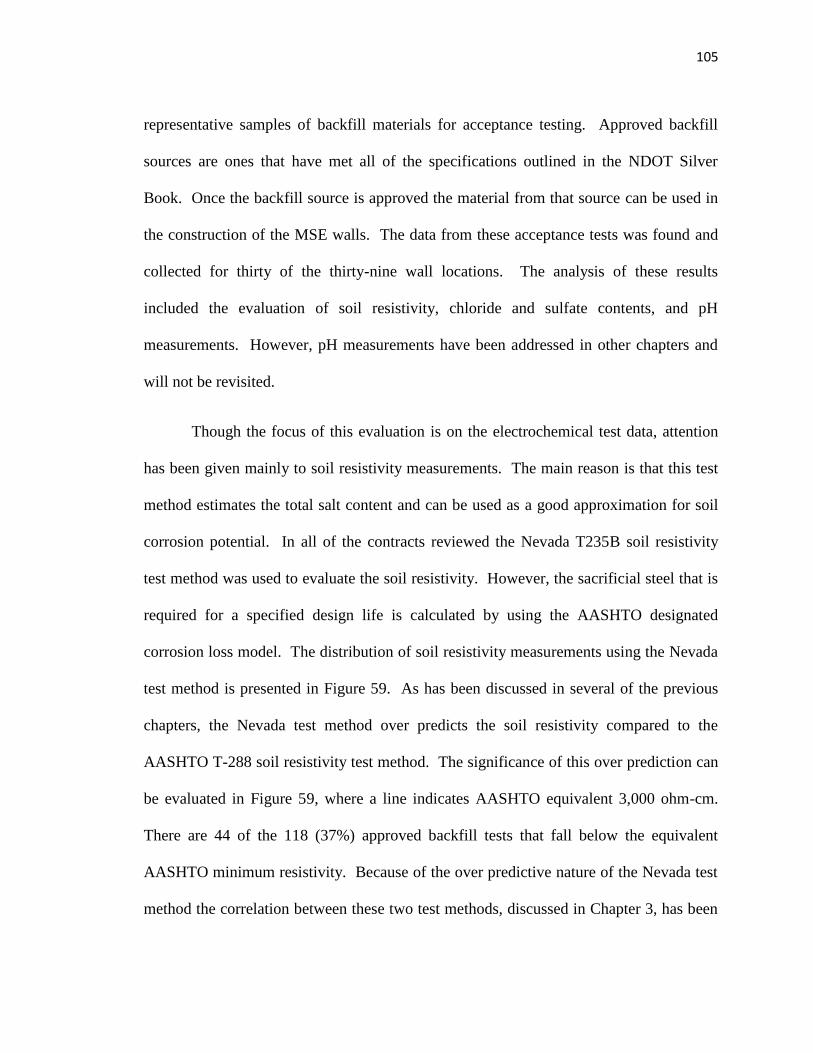
105

representative samples of backfill materials for acceptance testing. Approved backfill

sources are ones that have met all of the specifications outlined in the NDOT Silver

Book. Once the backfill source is approved the material from that source can be used in

the construction of the MSE walls. The data from these acceptance tests was found and

collected for thirty of the thirty-nine wall locations. The analysis of these results

included the evaluation of soil resistivity, chloride and sulfate contents, and pH

measurements. However, pH measurements have been addressed in other chapters and

will not be revisited.

Though the focus of this evaluation is on the electrochemical test data, attention

has been given mainly to soil resistivity measurements. The main reason is that this test

method estimates the total salt content and can be used as a good approximation for soil

corrosion potential. In all of the contracts reviewed the Nevada T235B soil resistivity

test method was used to evaluate the soil resistivity. However, the sacrificial steel that is

required for a specified design life is calculated by using the AASHTO designated

corrosion loss model. The distribution of soil resistivity measurements using the Nevada

test method is presented in Figure 59. As has been discussed in several of the previous

chapters, the Nevada test method over predicts the soil resistivity compared to the

AASHTO T-288 soil resistivity test method. The significance of this over prediction can

be evaluated in Figure 59, where a line indicates AASHTO equivalent 3,000 ohm-cm.

There are 44 of the 118 (37%) approved backfill tests that fall below the equivalent

AASHTO minimum resistivity. Because of the over predictive nature of the Nevada test

method the correlation between these two test methods, discussed in Chapter 3, has been

106

applied to these data sets as well; thus allowing an equivalent AASHTO soil resistivity

estimate. It is apparent from this figure that there are a significant number of approved

backfills, which are considered corrosive to very corrosive may have been used as the

MSE wall backfill in Nevada.

The AASHTO resistivity estimates (Equation 3.1) of the thirty wall locations

where test data was found are presented in Figure 60. The maximum, minimum, and

average values reported are presented so that the range of values can be seen. The wall

construction has also been divided into decades so that one can evaluate which walls are

older. While the test data represents the samples that were submitted and approved for

use, the data does not necessarily represent the backfill that was used, as seen in the

statistical analysis of the Flamingo and Cheyenne backfill data. A contractor could

supply several samples for source approval. Many of those sources can be approved, but

the contractor may only use a few of them. What is unknown is, once the approval

process is completed whether the contractor used the approved soils with higher or lower

resistivity values. These results can be used as a starting point for the wall prioritization

process. It is also interesting to note that for the Flamingo and Cheyenne data, both

approval data from prior to construction and subsequent on-site investigation data have

been included as a frame of reference for potential variation in backfill characteristics.

These sets of data can be used as anchoring points when evaluating other walls because

both of these walls had approval data during construction, while their more recent on-site

investigation data falls significantly below the original data.

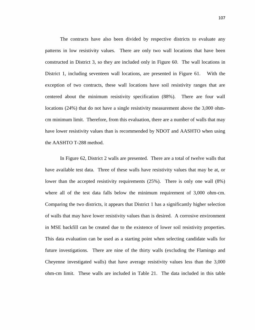
107

The contracts have also been divided by respective districts to evaluate any

patterns in low resistivity values. There are only two wall locations that have been

constructed in District 3, so they are included only in Figure 60. The wall locations in

District 1, including seventeen wall locations, are presented in Figure 61. With the

exception of two contracts, these wall locations have soil resistivity ranges that are

centered about the minimum resistivity specification (88%). There are four wall

locations (24%) that do not have a single resistivity measurement above the 3,000 ohm-

cm minimum limit. Therefore, from this evaluation, there are a number of walls that may

have lower resistivity values than is recommended by NDOT and AASHTO when using

the AASHTO T-288 method.

In Figure 62, District 2 walls are presented. There are a total of twelve walls that

have available test data. Three of these walls have resistivity values that may be at, or

lower than the accepted resistivity requirements (25%). There is only one wall (8%)

where all of the test data falls below the minimum requirement of 3,000 ohm-cm.

Comparing the two districts, it appears that District 1 has a significantly higher selection

of walls that may have lower resistivity values than is desired. A corrosive environment

in MSE backfill can be created due to the existence of lower soil resistivity properties.

This data evaluation can be used as a starting point when selecting candidate walls for

future investigations. There are nine of the thirty walls (excluding the Flamingo and

Cheyenne investigated walls) that have average resistivity values less than the 3,000

ohm-cm limit. These walls are included in Table 21. The data included in this table

108

presents the salt content data ranges as well, in order to further fine-tune the selection

process.

The test results from the soluble salts, including chlorides and sulfates have been

included in Figures 63 and 64, respectively. A vast majority of the test samples fall

below the minimum limits recommended relative to soluble salts. Only twenty-five

contracts have been included here. Five of the thirty contracts with resistivity data did

not have soluble salt data. This is because the resistivity values were greater than 5,000

ohm-cm. The current practice is to waive the soluble salt testing requirements if the

resistivity is above this value. Therefore, five contracts do not have this data for any of

their approved samples. Only one wall location, not including the Flamingo walls, has

chloride values greater than the current maximum 100ppm limit while two wall locations

(excluding the Flamingo walls) are above the sulfate maximum limit of 200ppm. These

walls also had very low resistivity values, as is seen in Table 21.

From these figures a better prediction can be made regarding which walls should

be evaluated in the continuing Phase II study of MSE wall corrosion. Comparing the data

of the Flamingo and Cheyenne case histories with the data of other contracts, it is

possible to evaluate the likelihood of other walls that may be experiencing higher rates of

corrosion. The list of wall locations in Table 21 presents a starting point for this

evaluation.

The issue of wall age is important. More concern should be given to older walls

that with higher rates of corrosion will have serious limitations on their service lives. On

109

the other hand, newer walls offer the opportunity to be evaluated with less concern for

short term failure, where monitoring techniques would provide estimates of service life

reduction before issues related to mitigation are required.

As was seen in the Flamingo walls, twenty years can be considered the service

life of a wall constructed with aggressive soils. There are two other wall locations in Las

Vegas that are older than the Flamingo walls. One of these walls is on the list of

potential walls to be investigated because of the potentially aggressive backfill. The

other wall was constructed prior to some of the materials testing requirements that were

imposed in backfill approval processes. Due to the apparent aggressiveness of soils in

Las Vegas, the walls constructed (year 1981) under Contract 1916 should be considered

as well. Both of these wall locations are over twenty-five years old and the approval test

results for backfill used in Contract 1918 are considered corrosive.

Soil reinforcement type should also be a consideration when prioritizing which

MSE wall locations to investigate. The walls from Table 21 have been included in Table

22 which details the soil reinforcement type at each wall location. This table also

includes Contract 1916, which was identified above as having a high probability for

higher than anticipated rates of corrosion. By chance four wall locations with galvanized

tie strip reinforcements and four wall locations with galvanized WWF reinforcements

have been identified. There are two wall locations where the soil reinforcement types

have not been identified. Eight of the ten wall locations are located in the Las Vegas

area. Soil reinforcement type is a factor in corrosion mechanisms since one

reinforcement type may perform better than another.

110

The three MSE wall locations that were constructed prior to any of the Las Vegas

walls include two wall locations on State Route 431 on the Mount Rose Highway and the

first walls constructed in Nevada in Lovelock. None of these contracts included materials

testing data for the backfills used. The two wall locations on State Route 431 were likely

constructed using decomposed granite backfill because of material availability in that

area. The walls constructed in Lovelock in 1974 were investigated a few years ago. No

personnel at NDOT could locate the report or conclusions from the report regarding this

investigation. However, their general consensus was that the walls and soil

reinforcements were found to be in good condition. From these findings it can be

assumed that the walls constructed prior to Contract 1916 should not be the focus for

further immediate investigation.

There are two walls that should be included in the list for monitoring efforts. The

first is the other Flamingo walls where corrosion issues have already been identified and

monitoring stations have been installed. The second wall location should be the

remaining Cheyenne walls. The removed wall section had high rates of corrosion.

Therefore it is likely that other walls at that location should be evaluated. Table 23 ranks

all of the walls that had soil resistivity average values that fell below the minimum soil

resistivity requirements when the AASHTO correlation was used. Once the walls have

been ranked a work plan can be developed. Suggested practices are detailed below.

Recommendations have been included in the final chapter regarding which methods the

author suggests for each wall in future investigations.

111

6.2 Methods for Future Evaluation of Existing MSE Walls

Once the MSE wall locations are selected there are several methods of analysis

that can be used. Direct observation of the outside of the wall is not likely to be useful.

During the site visits conducted by the author it was observed that even walls such as the

Flamingo walls did not show outward signs of distress that could be directly related to

corrosion. There were instances where walls were not exactly vertical, but these could be

cases created during construction. There are four groups of evaluation methods that will

be identified in this research. Each of these methods has its own usefulness, but some

will be more costly than others. The four groups of evaluation methods for existing walls

include representative backfill soil testing, installation of non-stressed soil

reinforcements, nondestructive monitoring methods, and destructive direct observational

methods.

6.2.1 Representative Backfill Soil Testing

A review of the electrochemical properties measured at the Flamingo and

Cheyenne MSE wall case studies shows that the backfill that was used in MSE wall

construction is statistically different from the approved backfill for several of the

properties evaluated. When this understanding is extrapolated, there may be other walls

that could be in similar conditions. After selecting wall locations that warrant further

investigation, the first step in analysis is to identify a more accurate representation of the

electrochemical and physical properties of the soils of in-place backfills. While the

methods of evaluating the electrochemical properties have been discussed in previous

112

chapters, the methods for obtaining a statistically significant number of samples have not

been introduced. With the variation of soil characteristics that is likely to occur in the

backfill for these walls, it is important to obtain a representative number of samples that

will be needed to address the variability that can be expected.

A power analysis was used to identify the number of samples required to obtain

representative sampling (Fernandez 2009). The resistivity results from the Flamingo wall

data were used because the original approved backfill dataset was found to be statistically

different from the 2005 investigation backfill dataset. A coefficient of variation (COV)

of each sample set was calculated. The 1985 dataset has a COV of 33.6% and the 2005

dataset has a COV of 106%. The later value is too large to develop any meaningful

sampling statements. Because of the large variations in data and the relatively small data

sets it was decided to perform a logarithmic transformation on the data and recalculate

the COVs. After a logarithmic transform the resulting COVs are 4.47% and 13.9% for

the 1985 and 2005 data, respectively. Using these values in a power analysis can yield a

number of samples that should be tested in order to have a sample power of 0.80 or

greater. The transformed data suggest that nine samples are needed for a sample power

greater than 0.80, while twelve samples are required for a sample power greater than 0.90

(Figure 65).

The samples retrieved from the Flamingo MSE wall backfill were obtained from

behind all three walls. There are a total of 29,100 square feet of facing and 16,100 cubic

yards of backfill used at the three Flamingo MSE walls. The number of samples obtained

from the Flamingo MSE walls can be normalized with respect to either of these values in

113

order to identify the number of samples required for statistically meaningful sampling

programs at other walls. If the square footage of facing is used, three samples should be

collected from each 10,000 square feet of facing for a sample power of 0.80 and four

samples should be collected from each 10,000 square feet of facing for a sample power of

0.90.

A general rule of thumb for sample testing suggests that three samples should be

the minimum number collected. As was mentioned on several occasions, there are no

precision and bias statements to use in evaluation of test results for the AASHTO

resistivity method. Therefore, more samples are required in order to ensure that the

variability in the backfill and testing procedures are reduced. A reduction in sensitivity

has also been introduced in the use of a logarithmic transformation of the data. With

these issues of variability and sensitivity, it is recommended that the results from the

power analysis are doubled. This author suggests that six samples are retrieved per

10,000 square feet of wall facing. This will reduce the likelihood of misidentifying

backfill characteristics that are different from the originally approved backfill.

The sampling of backfill soils will likely be conducted using test boring

equipment. The methods of sampling will be similar to those used in current

geotechnical soil exploration practices. It should be kept in mind that the active wedge

interface starting at a distance equal one third of the wall height behind the wall face is a

critical area regarding corrosion. Sampling should be random in location with emphasis

given to this critical area. Consideration should also be given to depth into the backfill

and location along the walls. Field observations will need to be made regarding sample

114

similarities to other samples collected and types of materials collected. Future statistical

evaluation will be required when several samples appear to be dissimilar in gradation and

appearance.

Further modification of this specification can be made as the variation in

measurements is reduced. In general, an assumption of homogeneity is made regarding

the backfill at each wall location. However, there are many wall locations where several

walls have been constructed and large quantities of backfill were required. There is a

possibility that some of these wall MSE walls may have been constructed with backfill

from several sources, thus creating a need to use a block sampling evaluation.

6.2.2 Installation of Non-Stressed Soil Reinforcements

Since 1979, Caltrans has included inspection rods (or coupons) into their MSE

wall backfills (Jackura et al. 1987). It was the practice of systematically evaluating these

inspection rods that allowed them to identify the Mariposa wall (Chapter 2) that was

experiencing higher than anticipated corrosion rates. During the Flamingo investigation

there were “dummy” coupons installed into the backfill so that corrosion evaluations

could continue (Fishman 2005). One option that can assist in identifying other NDOT

MSE walls that are experiencing higher rates of corrosion is to install both galvanized

and bare steel inspection rods or coupons that are not part of the structural components of

the MSE walls with the provision that they can be removed at specified time intervals. It

is suggested that the Caltrans method, which has proved to be successful, be used for the

evaluation of corrosion. It is recommended that NDOT develop a monitoring procedure

115

and evaluation as a part of their highway/bridge maintenance program to evaluate the

corrosion status of these coupons on a regular basis.

An important issue is that these inspection rods should be evaluated by direct

observation. Both galvanized and bare steel samples should be used so that the rate of

corrosion of each material can be evaluated. This will also enable the prediction of

corrosion of galvanized steel once the protective coating has been depleted. It is

important to keep some of the corrosion behaviors presented in Chapter 3 in mind when

evaluating the bare steel samples in the early years because of passivity effects. The next

section will introduce the use of nondestructive blind measurements, but those methods

produce a uniform corrosion rate estimate. As has been seen in the Flamingo and

Cheyenne walls, a uniform measurement is not a conservative estimate of what is actually

occurring in the backfill. However, the estimates of uniform corrosion rate can be useful

in providing an estimate of the average corrosion and can also bracket that estimate.

6.2.3 Nondestructive Monitoring Methods

There are a large number of publications and articles that have addressed the use

of indirect measurements of corrosion in MSE backfill. The current FHWA manual on

corrosion and degradation of MSE wall soil reinforcements commits a whole chapter to

this issue (Elias 2000). There are also other publications that present methods of

installation and observation for polarization resistance (PR) monitoring and half-cell

potential measurements (Elias 2000). The existing MSE wall soil reinforcements that are

under investigation can be connected to these devices in order to make measurements and

116

evaluations. However, there are numerous publications that specify that these

measurements need to be carefully analyzed so that interpretations are more accurate.

The issue is that there is no baseline reading that was performed at the initial installation

of the soil reinforcement (NCHRP 24-28 2007). Without this baseline measurement the

person evaluating the measurements has to make an assumption about the original state

of the steel reinforcement.

One method of using the indirect measurement techniques is to couple it with the

previous method of observation rods and “dummy” coupons. Using direct observations

with PR monitoring can be a very useful method of evaluation. The observation rods can

be extracted at intervals of several years while the PR monitoring measurements are

taken at seasonal intervals. The combination of these two methods can be a powerful tool

in corrosion rate estimation.

6.2.4 Destructive Direct Observational Methods

The final of the four general methods for estimating corrosion involves

destructive testing. Both the Flamingo and Cheyenne walls were investigated using

destructive methods. Advancing test pits into the MSE wall backfill, either at the top or

into the facing, is required to make direct observations of the soil reinforcements. This is

a method that should be considered as a last resort. After using the previous three

methods in concert to identify walls that have experienced higher rates of corrosion, this

destructive method can be used to identify the severity of the corrosion. Once the

severity is evaluated, mitigation efforts can be undertaken. Proper implementation of the

117

first three methods can reduce the potential possibility that a wall needs to be investigated

in this destructive manner.

6.3 Future MSE Wall Investigation Recommendations

There are a number of walls that have presented themselves as potential

candidates for future evaluation. Methods for these future evaluations are also presented

in this chapter. The evaluation process can be performed in a series of steps, starting with

the lowest expense and increasing as the evaluation continues. The first step will be to

identify the corrosive nature of the backfill that has been used in the construction of these

walls. The method for analysis has been referred to in Section 6.2.1 above. One clear

finding from the Flamingo and Cheyenne backfill analyses is that the corrosive nature of

the soils used as backfill were not clearly identified during the construction process. The

existing backfills need to be evaluated prior to any further wall evaluation.

Once the backfill at a specific wall location is truly identified as corrosive the

evaluation should progress to step two, identified in Section 6.2.2, which involves the

installation of monitoring devices. This is especially useful for the more recently

constructed MSE walls as corrosion assessment of coupons and PR measurements can be

monitored over a longer period of time. However, the older walls, constructed in the

1980s should be considered higher risk walls, and should be treated accordingly. It is

clear that the existing two Flamingo walls will not have service lives of seventy-five

years, even if less conservative estimates of loss are used. Even though the two wall

locations in Las Vegas that are older than the Flamingo walls and have been constructed

118

using galvanized soil reinforcements, they are suspect if their backfill soils are found to

be corrosive in step one of the investigation.

The more recent walls offer a great opportunity for proactive predictions of

corrosion rates and should be treated as such. They should be monitored regularly once

their in-place backfills have been evaluated and found to be corrosive. The corrosive

nature of Nevada’s soils has been clearly documented and the MSE walls that have been

constructed should be evaluated further so that potentially catastrophic failures can be

avoided in the future.

119

Chapter Seven

Conclusion and Recommendations

Mechanically stabilized earth walls are a practical solution as retaining structure,

and have been incorporated in a large number of NDOT projects resulting in over 150

walls in Nevada. However, as is commonly practiced with other structures, these

retaining walls require periodic monitoring and performance evaluations. It appears that

corrosion monitoring is an important component in the successful performance of MSE

walls. As has been noted several times in this report, exterior evaluations or observations

of wall facing during site visits are not a sufficient method for corrosion monitoring.

This is especially true because no baseline comparison of deformation measurements

exists. Corrosion monitoring can only be conducted by evaluation of the soil and

reinforcement conditions behind the wall facing. This is evidenced by the fact that two

MSE wall locations (I-515/Flamingo and I-15/Cheyenne intersections) have been found

to have high rates of corrosion that directly affect their abilities to perform adequately

over their designated service lives. One of the three MSE walls at the Flamingo

intersection has been retrofitted with a cast-in-place tie-back wall, at a great expense due

to the effects of high levels of corrosion on the soil reinforcements. Only accidental

discovery of corroded reinforcements led to these discoveries. Outward observations of

these walls showed no signs of distress that would lead to the conclusion that the soil

reinforcements were experiencing detrimental loss in cross sectional area due to

corrosion. These higher rates of corrosion were produced for both galvanized and bare

steel reinforcements demonstrating that galvanized MSE wall reinforcements are also

subject to advanced corrosion in Nevada.

120

The Flamingo and Cheyenne wall corrosion issues are well documented and

identified. However, the question now is, how many other walls in Nevada are

experiencing higher than anticipated rates of corrosion. This is not a simple question to

answer and the investigation attempts to answer this important question. There is

significant potential for other walls to have high rates of corrosion because of the

unintentional use of aggressive MSE backfill in Nevada. The use of the Nevada T235B

test method, which over predicts the soil resistivity, has allowed the use of more

corrosive soils in Nevada MSE walls. The Nevada T235B test method measures the

conductivity of water from a saturated backfill soil solution. This method of resistivity

measurement is significantly different from the AASHTO T-288 test method which uses

a soil box to measure backfill resistivity directly. A correlation between the Nevada

T235B and AASHTO T-288 resistivity test methods shows that the Nevada test method

is not conservative with respect to identifying aggressive soils. Because of this, the

corrosive nature of the backfill used in other Nevada MSE walls has been reevaluated.

The results in Chapter 6 show that there are at least nine more MSE wall locations that

may have been constructed with aggressive soils. The use of these aggressive soils

directly affects the internal stability of these walls and these walls need to be investigated

further.

The originally approved backfill test data for the Flamingo MSE walls is

misleading in its characterization of the aggressiveness of the backfill, which was

subsequently demonstrated by MMCE. This provides the need for the immediate

evaluation of other Nevada walls. This is substantiated by the statistical analysis of

121

backfill properties in this report. The statistical analysis focused on the electrochemical

properties of the initially approved backfill for the Flamingo and Cheyenne case studies

and compared that to the properties of the backfill that was actually used in the

construction of the walls. The results from this analysis show that the characterization of

backfill approved during construction did not effectively predict the corrosive nature of

the backfill that was used in MSE wall construction. Because this method of backfill

approval has been widely used in Nevada, this practice needs reevaluation as this may

have occurred at other Nevada wall locations. Statistical methods for obtaining

representative samples are presented so that effective characterization that includes the

variability in corrosive material properties can be accounted for.

Recommendations

The recommendations for the future can be divided into two main categories. It is

recommended that existing MSE walls in Nevada be evaluated for the potentially

detrimental effects of corrosive backfill. It is also recommended the newly adopted

practices by NDOT regarding the approval of MSE backfill (production testing) be

included as a requirement in future MSE wall construction. The support for these

recommendations has been developed within this report and will be summarized below.

Two MSE wall locations with high rates of corrosion were identified completely

by accident. It is now clear that there are other walls in the NDOT inventory that are

likely to be in the same condition. Twelve of the best candidate wall locations have been

122

identified in Chapter 6 (Table 23). An investigation of these MSE walls should include

the following four recommendations:

1. Representative backfill soil testing – all walls should be evaluated to ensure

proper characterization of the backfill (i.e. project testing) that was used during

construction (Section 6.2.1);

2. Installation of non-stressed (dummy) soil reinforcements in newer walls and as

needed in most critical existing walls (as identified in this report – see Table 23)

– reinforcement coupons should be installed so that baseline loss measurements

can be estimated (Section 6.2.2);

3. Nondestructive monitoring methods – monitoring of corrosion loss, especially

including the Flamingo walls, which have monitoring stations already, should be

conducted (Section 6.2.3). It is recommended that NDOT develop a monitoring

procedure and evaluation as a part of their highway/bridge maintenance program

to evaluate the corrosion status of these coupons on a regular basis (e.g. Caltrans

procedure).

4. Destructive direct observational methods – walls that are found to have aggressive

backfills (based on post-construction electrochemical testing of backfill soils)

should be investigated further for direct observation of soil reinforcements

(Section 6.2.4).

123

A combination of these four approaches would have a significant impact on the

safety of Nevada walls. The ability to monitor corrosion rates throughout the design life

of an MSE wall is strongly recommended given the history and findings of MSE wall

corrosion studies and the aggressive nature of the soils in Nevada. This proactive

approach will give NDOT the ability to prevent failures in its MSE walls caused by

internal stability due to high rates of corrosion.

124

References

AASHTO (1973). Standard Specifications for Highway Bridges, 11th

Edition. American

Association of State Highway and Transportation Officials, Washington D.C.


Edition. American



Edition. American



Edition. American



Edition. American



Edition. American


AASHTO (2007). LRFD Bridge Design Specifications, 4th

Edition. American


AMSE 2006. Reduced Zinc Loss Rate for Design of MSE Structures. Association of

Metallically Stabilized Earth, McLean, Virginia, 2006

ASM International. Metals Handbook, 9th

Edition. Vol. 13. Metals Park, Ohio, 1987.

Blake, William. Personal interview. February 20, 2009.

Blight, G.E. and M.S.W. Dane. “Deterioration of a Wall Complex Constructed of

Reinforced Earth.” Geotechnique Vol. 39.1. March 1989.

Darbin, M., J.M. Jailloux, and J. Montuelle. Durability of Reinforced Earth Structures:

The Results of a Long-term Study Conducted on Galvanized Steel. Proceedings –

Institution of Civil Engineers. Part 1 Design and Construction, Vol. 84. 1988.

Elias, Victor. Durability/Corrosion of Soil Reinforced Structures. FHWA-RD-89-186,

Washington D.C., 1990.

Elias, Victor. Corrosion/Degradation of Soil Reinforcements for Mechanically Stabilized

Earth Walls and Reinforced Soil Slopes. FHWA-NHI-00-044, Washington D.C., 2000.

Elias, Victor, Barry R. Christopher, and Ryan R. Berg, Mechanically Stabilized Earth

Walls and Reinforced Slopes Design and Construction Guidelines. FHWA-NHI-00-043,

Washington D.C., 2001.

Fernandez, George. SAS Applications (http://www.ag.unr.edu/gf/) 2009.

http://www.ag.unr.edu/gf/

125

Fishman, Kenneth L. Consultant’s Report: Corrosion Evaluation of MSE Walls I-

515/Flamingo Road Las Vegas, Nevada. McMahon & Mann Consulting Engineers, P.C.

May 2005.

Jackura, K.A., Gary A. Garofalo, and Darrell Beddard, Investigation of Corrosion at 14

Mechanically Stabilized Embankment Sites. Sacramento, California: California

Department of Transportation, 1987.

Kuehl, Robert O. Design of Experiments: Statistical Principles of Research Design and

Analysis, 2nd

Edition. New York: Duxbury, 2000.

NCHRP 24-28, LRFD Metal Loss and Service-Life Strength Reduction Factors for Metal

Reinforced Systems in Geotechnical Applications, Phase 1 Interim Report. April 2007.

NDOT (1968), Standard Specifications for Road and Bridge Construction. Nevada

Department of Transportation, Carson City, Nevada, 1968.









Porter, Frank C. Corrosion Resistance of Zinc and Zinc Alloys. New York: Marcel

Dekker, 1994.

Raeburn, Christopher L. M. Murat Monkul, and Marvin R. Piles. Evaluation of Corrosion

of Metallic Reinforcements and connections in MSE Retaining Walls, Project 643.

FHWA-OR-RD-08-10, Washington D.C. 2008.

Romanoff, Melvin. Underground Corrosion. National Bureau of Standards Circular 579.

Houston: National Association of Corrosion Engineers, 1989

Scully, J.C. The Fundamentals of Corrosion, 3rd

Edition. Oxford: Pergamon, 1990.

Thornley, John D. Use of Statistical Methods to Study Corrosion Aggressiveness at

Nevada Mechanically Stabilized Earth Wall Sites. Thesis, University of Nevada, 2009.

Ann Arbor: UMI, 2009.

Zhang, Xiaoge Gregory. Corrosion and Electrochemistry of Zinc. New York: Plenum,

1996.

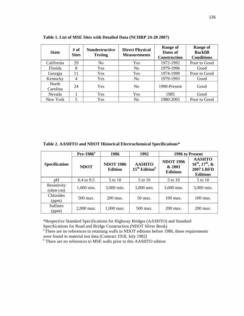
126

Table 1. List of MSE Sites with Detailed Data (NCHRP 24-28 2007)

State # of

Sites

Nondestructive

Testing

Direct Physical

Measurements

Range of

Dates of

Construction

Range of

Backfill

Conditions

California 29 No Yes 1972-1992 Poor to Good

Florida 8 Yes No 1979-1996 Good

Georgia 11 Yes Yes 1974-1990 Poor to Good

Kentucky 4 Yes No 1979-1993 Good

North

Carolina 24 Yes No 1990-Present Good

Nevada 1 Yes Yes 1985 Good

New York 5 Yes No 1980-2005 Poor to Good

Table 2. AASHTO and NDOT Historical Electrochemical Specifications*

Specification

Pre-1986a

1986 1992 1996 to Present

NDOT NDOT 1986

Edition

AASHTO

15th

Editionb

NDOT 1996

& 2001

Editions

AASHTO

16th

, 17th

, &

2007 LRFD

Editions

pH 6.4 to 9.5 5 to 10 5 to 10 5 to 10 5 to 10

Resistivity

(ohm-cm) 1,000 min. 3,000 min. 3,000 min. 3,000 min. 3,000 min.

Chlorides

(ppm) 500 max. 200 max. 50 max. 100 max. 100 max.

Sulfates

(ppm) 2,000 max. 1,000 max. 500 max. 200 max. 200 max.

*Respective Standard Specifications for Highway Bridges (AASHTO) and Standard

Specifications for Road and Bridge Construction (NDOT Silver Book) a There are no references to retaining walls in NDOT editions before 1986, these requirements

were found in material test data (Contract 1918, July 1982) b There are no references to MSE walls prior to this AASHTO edition

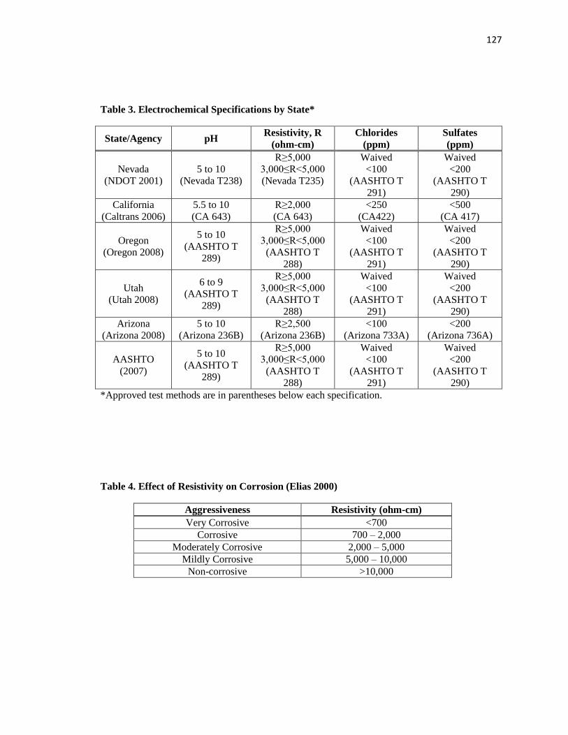
127

Table 3. Electrochemical Specifications by State*

State/Agency pH Resistivity, R

(ohm-cm)

Chlorides

(ppm)

Sulfates

(ppm)

Nevada

(NDOT 2001)

5 to 10

(Nevada T238)

R≥5,000

3,000≤R<5,000

(Nevada T235)

Waived

<100

(AASHTO T

291)

Waived

<200

(AASHTO T

290)

California

(Caltrans 2006)

5.5 to 10

(CA 643)

R≥2,000

(CA 643)

<250

(CA422)

<500

(CA 417)

Oregon

(Oregon 2008)

5 to 10

(AASHTO T

289)

R≥5,000

3,000≤R<5,000

(AASHTO T

288)

Waived

<100

(AASHTO T

291)

Waived

<200

(AASHTO T

290)

Utah

(Utah 2008)

6 to 9

(AASHTO T

289)

R≥5,000

3,000≤R<5,000

(AASHTO T

288)

Waived

<100

(AASHTO T

291)

Waived

<200

(AASHTO T

290)

Arizona

(Arizona 2008)

5 to 10

(Arizona 236B)

R≥2,500

(Arizona 236B)

<100

(Arizona 733A)

<200

(Arizona 736A)

AASHTO

(2007)

5 to 10

(AASHTO T

289)

R≥5,000

3,000≤R<5,000

(AASHTO T

288)

Waived

<100

(AASHTO T

291)

Waived

<200

(AASHTO T

290)

*Approved test methods are in parentheses below each specification.

Table 4. Effect of Resistivity on Corrosion (Elias 2000)

Aggressiveness Resistivity (ohm-cm)

Very Corrosive <700

Corrosive 700 – 2,000

Moderately Corrosive 2,000 – 5,000

Mildly Corrosive 5,000 – 10,000

Non-corrosive >10,000

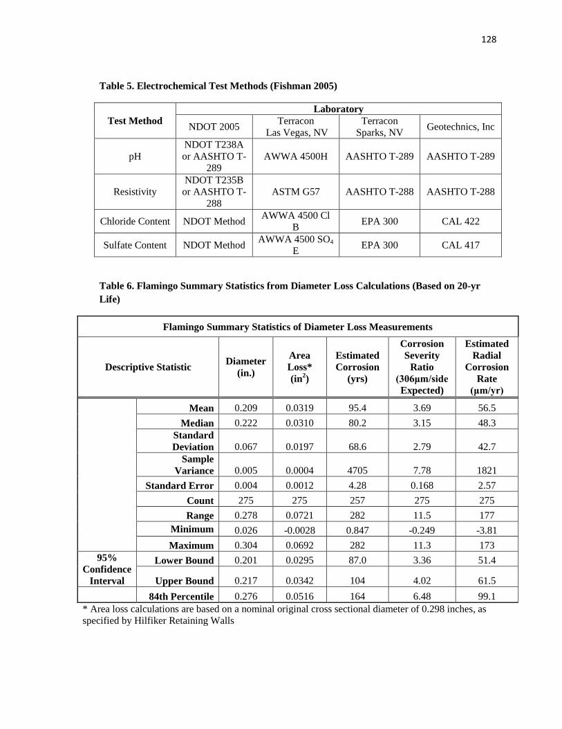
128

Table 5. Electrochemical Test Methods (Fishman 2005)

Test Method

Laboratory

NDOT 2005 Terracon

Las Vegas, NV

Terracon

Sparks, NV Geotechnics, Inc

pH

NDOT T238A

or AASHTO T-

289

AWWA 4500H AASHTO T-289 AASHTO T-289

Resistivity

NDOT T235B

or AASHTO T-

288

ASTM G57 AASHTO T-288 AASHTO T-288

Chloride Content NDOT Method AWWA 4500 Cl

B EPA 300 CAL 422

Sulfate Content NDOT Method AWWA 4500 SO4

E EPA 300 CAL 417

Table 6. Flamingo Summary Statistics from Diameter Loss Calculations (Based on 20-yr

Life)

Flamingo Summary Statistics of Diameter Loss Measurements

Descriptive Statistic Diameter

(in.)

Area

Loss*

(in2)

Estimated

Corrosion

(yrs)

Corrosion

Severity

Ratio

(306μm/side

Expected)

Estimated

Radial

Corrosion

Rate

(μm/yr)

Mean 0.209 0.0319 95.4 3.69 56.5

Median 0.222 0.0310 80.2 3.15 48.3

Standard

Deviation 0.067 0.0197 68.6 2.79 42.7

Sample

Variance 0.005 0.0004 4705 7.78 1821

Standard Error 0.004 0.0012 4.28 0.168 2.57

Count 275 275 257 275 275

Range 0.278 0.0721 282 11.5 177

Minimum 0.026 -0.0028 0.847 -0.249 -3.81

Maximum 0.304 0.0692 282 11.3 173

95%

Confidence

Interval

Lower Bound 0.201 0.0295 87.0 3.36 51.4

Upper Bound 0.217 0.0342 104 4.02 61.5

84th Percentile 0.276 0.0516 164 6.48 99.1

* Area loss calculations are based on a nominal original cross sectional diameter of 0.298 inches, as

specified by Hilfiker Retaining Walls

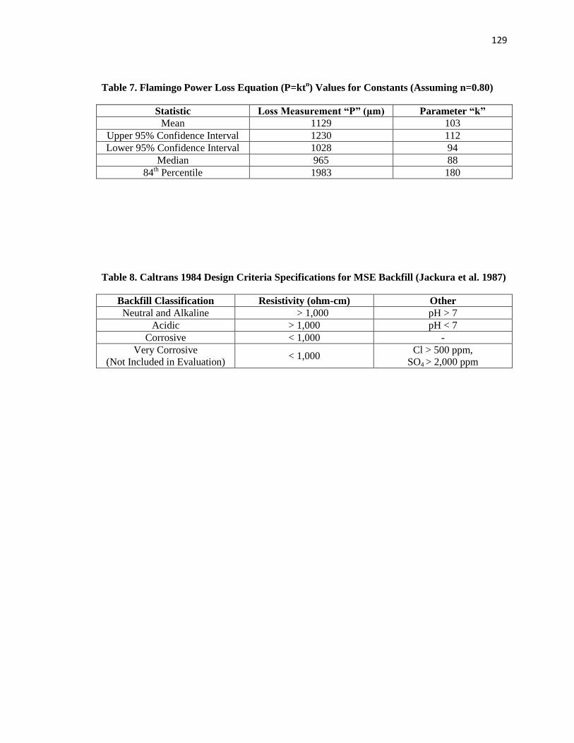
129

Table 7. Flamingo Power Loss Equation (P=ktn) Values for Constants (Assuming n=0.80)

Statistic Loss Measurement “P” (μm) Parameter “k”

Mean 1129 103

Upper 95% Confidence Interval 1230 112

Lower 95% Confidence Interval 1028 94

Median 965 88

84th Percentile 1983 180

Table 8. Caltrans 1984 Design Criteria Specifications for MSE Backfill (Jackura et al. 1987)

Backfill Classification Resistivity (ohm-cm) Other

Neutral and Alkaline > 1,000 pH > 7

Acidic > 1,000 pH < 7

Corrosive < 1,000 -

Very Corrosive

(Not Included in Evaluation) < 1,000

Cl > 500 ppm,

SO4 > 2,000 ppm

130

Tab

le 9

. 19

85

Ap

pro

ved

Ba

ckfi

ll w

ith

Sp

ecif

icati

on

Com

pari

son

s

Shad

ed c

ells

did

no

t pas

s.

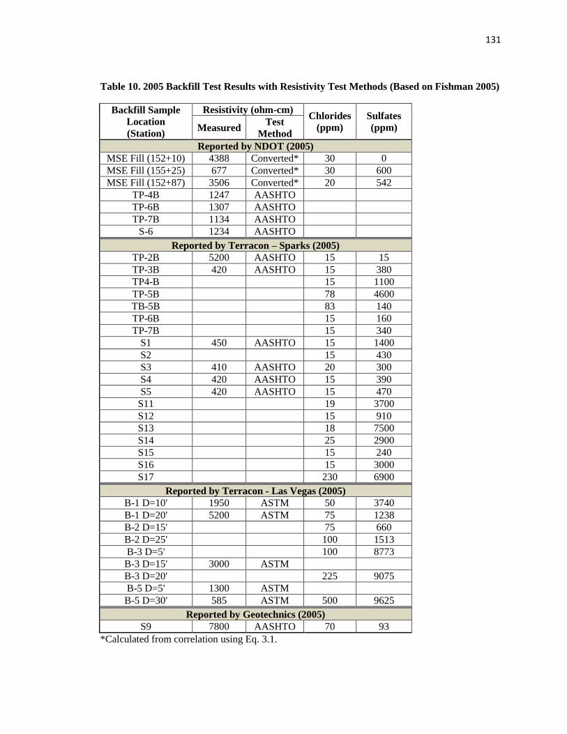
131

Table 10. 2005 Backfill Test Results with Resistivity Test Methods (Based on Fishman 2005)

Backfill Sample

Location

(Station)

Resistivity (ohm-cm) Chlorides

(ppm)

Sulfates

(ppm) Measured Test

Method

Reported by NDOT (2005)

MSE Fill (152+10) 4388 Converted* 30 0



TP-4B 1247 AASHTO

TP-6B 1307 AASHTO

TP-7B 1134 AASHTO

S-6 1234 AASHTO

Reported by Terracon – Sparks (2005)

TP-2B 5200 AASHTO 15 15

TP-3B 420 AASHTO 15 380

TP4-B 15 1100

TP-5B 78 4600

TB-5B 83 140

TP-6B 15 160

TP-7B 15 340

S1 450 AASHTO 15 1400

S2 15 430

S3 410 AASHTO 20 300

S4 420 AASHTO 15 390

S5 420 AASHTO 15 470

S11 19 3700

S12 15 910

S13 18 7500

S14 25 2900

S15 15 240

S16 15 3000

S17 230 6900

Reported by Terracon - Las Vegas (2005)

B-1 D=10' 1950 ASTM 50 3740

B-1 D=20' 5200 ASTM 75 1238

B-2 D=15' 75 660

B-2 D=25' 100 1513

B-3 D=5' 100 8773

B-3 D=15' 3000 ASTM

B-3 D=20' 225 9075

B-5 D=5' 1300 ASTM

B-5 D=30' 585 ASTM 500 9625

Reported by Geotechnics (2005)

S9 7800 AASHTO 70 93

*Calculated from correlation using Eq. 3.1.

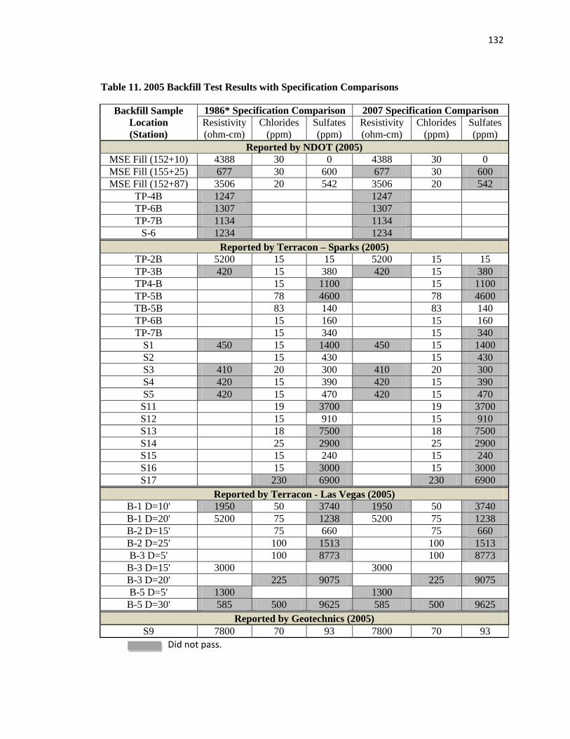
132

Table 11. 2005 Backfill Test Results with Specification Comparisons

Backfill Sample

Location

(Station)

1986* Specification Comparison 2007 Specification Comparison

Resistivity

(ohm-cm)

Chlorides

(ppm)

Sulfates

(ppm)

Resistivity

(ohm-cm)

Chlorides

(ppm)

Sulfates

(ppm)

Reported by NDOT (2005)

MSE Fill (152+10) 4388 30 0 4388 30 0

MSE Fill (155+25) 677 30 600 677 30 600

MSE Fill (152+87) 3506 20 542 3506 20 542

TP-4B 1247 1247

TP-6B 1307 1307

TP-7B 1134 1134

S-6 1234 1234

Reported by Terracon – Sparks (2005)

TP-2B 5200 15 15 5200 15 15

TP-3B 420 15 380 420 15 380

TP4-B 15 1100 15 1100

TP-5B 78 4600 78 4600

TB-5B 83 140 83 140

TP-6B 15 160 15 160

TP-7B 15 340 15 340

S1 450 15 1400 450 15 1400

S2 15 430 15 430

S3 410 20 300 410 20 300

S4 420 15 390 420 15 390

S5 420 15 470 420 15 470

S11 19 3700 19 3700

S12 15 910 15 910

S13 18 7500 18 7500

S14 25 2900 25 2900

S15 15 240 15 240

S16 15 3000 15 3000

S17 230 6900 230 6900

Reported by Terracon - Las Vegas (2005)

B-1 D=10' 1950 50 3740 1950 50 3740

B-1 D=20' 5200 75 1238 5200 75 1238

B-2 D=15' 75 660 75 660

B-2 D=25' 100 1513 100 1513

B-3 D=5' 100 8773 100 8773

B-3 D=15' 3000 3000

B-3 D=20' 225 9075 225 9075

B-5 D=5' 1300 1300

B-5 D=30' 585 500 9625 585 500 9625

Reported by Geotechnics (2005)

S9 7800 70 93 7800 70 93

Did not pass.

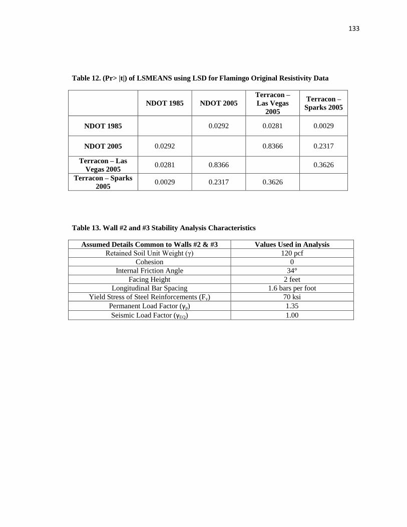
133

Table 12. (Pr> |t|) of LSMEANS using LSD for Flamingo Original Resistivity Data

NDOT 1985 NDOT 2005

Terracon –

Las Vegas

2005

Terracon –

Sparks 2005

NDOT 1985 0.0292 0.0281 0.0029

NDOT 2005 0.0292 0.8366 0.2317

Terracon – Las

Vegas 2005 0.0281 0.8366 0.3626

Terracon – Sparks

2005 0.0029 0.2317 0.3626

Table 13. Wall #2 and #3 Stability Analysis Characteristics

Assumed Details Common to Walls #2 & #3 Values Used in Analysis

Retained Soil Unit Weight (γ) 120 pcf

Cohesion 0

Internal Friction Angle 34°

Facing Height 2 feet

Longitudinal Bar Spacing 1.6 bars per foot

Yield Stress of Steel Reinforcements (Fy) 70 ksi

Permanent Load Factor (γp) 1.35

Seismic Load Factor (γEQ) 1.00

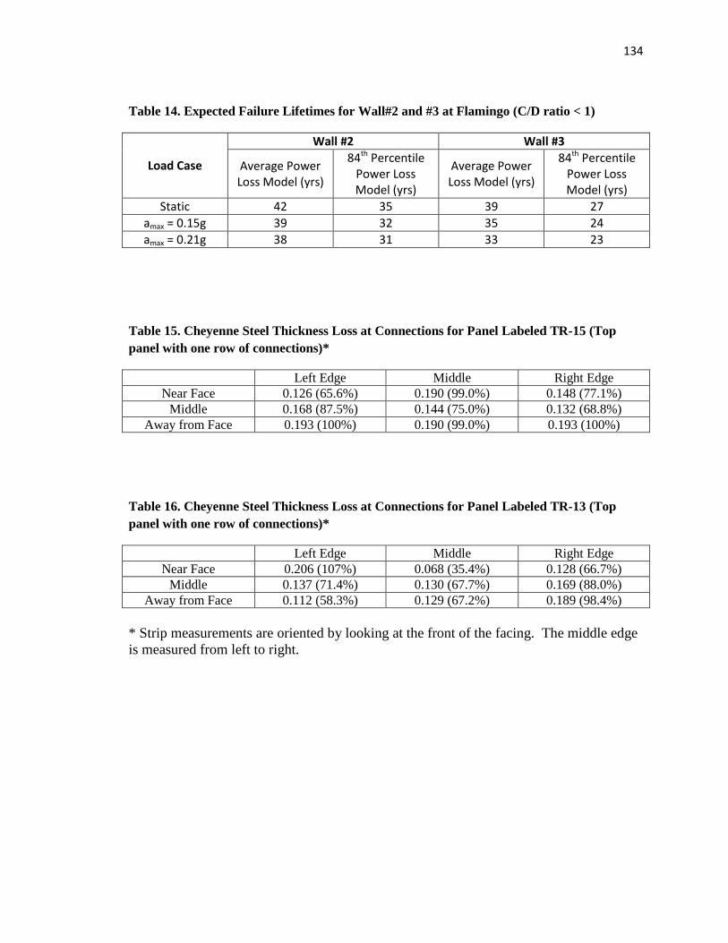
134

Table 14. Expected Failure Lifetimes for Wall#2 and #3 at Flamingo (C/D ratio < 1)

Load Case

Wall #2 Wall #3

Average Power Loss Model (yrs)

84th Percentile Power Loss Model (yrs)

Average Power Loss Model (yrs)

84th Percentile Power Loss Model (yrs)

Static 42 35 39 27

amax = 0.15g 39 32 35 24

amax = 0.21g 38 31 33 23

Table 15. Cheyenne Steel Thickness Loss at Connections for Panel Labeled TR-15 (Top

panel with one row of connections)*

Left Edge Middle Right Edge

Near Face 0.126 (65.6%) 0.190 (99.0%) 0.148 (77.1%)

Middle 0.168 (87.5%) 0.144 (75.0%) 0.132 (68.8%)

Away from Face 0.193 (100%) 0.190 (99.0%) 0.193 (100%)

Table 16. Cheyenne Steel Thickness Loss at Connections for Panel Labeled TR-13 (Top

panel with one row of connections)*

Left Edge Middle Right Edge

Near Face 0.206 (107%) 0.068 (35.4%) 0.128 (66.7%)

Middle 0.137 (71.4%) 0.130 (67.7%) 0.169 (88.0%)

Away from Face 0.112 (58.3%) 0.129 (67.2%) 0.189 (98.4%)

* Strip measurements are oriented by looking at the front of the facing. The middle edge

is measured from left to right.

135

Table 17. Cheyenne Summary Statistics from Thickness Loss Calculations (Based on 9-yr

Life)

Cheyenne Summary Statistics of Cross Sectional Loss Measurements

Descriptive Statistic Area

(in2)

Area

Loss*

(in2)

Estimated

Corrosion

(yrs)

Corrosion

Severity

Ratio

(54μm/side

Expected)

Estimated

Overall

Corrosion

Rate/Side

(μm/yr)

Mean 0.295 0.0573 39.4 6.83 41.0

Median 0.305 0.0475 34.9 5.66 34.0

Standard

Deviation 0.0396 0.0396 21.9 4.73 28.4

Sample

Variance 0.00157 0.00157 480 22.3 804

Standard

Error 0.00398 0.00398 2.21 0.475 2.85

Count 99 99 98 99 99

Range 0.170 0.170 99.7 20.2 121

Minimum 0.183 -3.99 E-05 0.107 -0.00733 -0.0440

Maximum 0.352 0.170 99.8 20.2 121

95%

Confidence

Interval

Lower Bound 0.287 0.0494 35.0 5.90 35.4

Upper Bound 0.303 0.0651 43.7 7.76 46.5

84th

Percentile 0.256 0.0969 61.3 11.6 69.3

* Area loss calculations are based on an average original cross sectional area of 0.3524 inches2, as

specified by Reinforced Earth Company design calculations

Table 18. Cheyenne Power Loss Equation (P=ktn) Values for Constants (Assuming n=0.65)

Statistic Loss Measurement “P”

(μm) Parameter “k”

Mean 369 88

Upper 95% Confidence Interval 419 100

Lower 95% Confidence Interval 318 76

Median 306 73

84th

Percentile 624 150

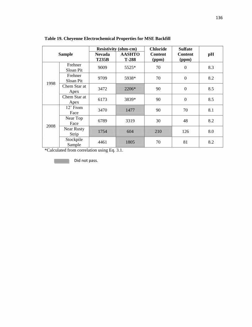
136

Table 19. Cheyenne Electrochemical Properties for MSE Backfill

Sample

Resistivity (ohm-cm) Chloride

Content

(ppm)

Sulfate

Content

(ppm)

pH Nevada

T235B

AASHTO

T-288

1998

Frehner

Sloan Pit 9009 5525* 70 0 8.3

Frehner

Sloan Pit 9709 5938* 70 0 8.2

Chem Star at

Apex 3472 2206* 90 0 8.5

Chem Star at

Apex 6173 3839* 90 0 8.5

2008

12’ From

Face 3470 1477 90 70 8.1

Near Top

Face 6789 3319 30 48 8.2

Near Rusty

Strip 1754 604 210 126 8.0

Stockpile

Sample 4461 1805 70 81 8.2

*Calculated from correlation using Eq. 3.1.

Did not pass.

137

Table 20. NDOT MSE Wall Database

Contract

Number

Date of

Drawing

Date of

Contract District County Intersection

No. of

Walls

Maximum

Height (ft.) Wall Manufacturer

Wall

Reinforcement

Type

3324 1-Aug-2006 16-Aug-2007 1 Clark SR 160 and Jones Blvd 6 45.1 Reco Tie Strips - galv.

3320 13-Jul-2006 21-Nov-2006 2 Storey

USA Parkway Truckee Bridge

(Storey County Side) 3 20 SSL WWF - galv.

3313 20-Jun-2008 1 Clark I-15 and Cheyenne Ave 1 15 Reco Tie Strips - galv.

3296 29-Nov-2005 3-Apr-2006 2 Carson

US 50 to Spooner Summit

(Underpass) 6 34 Reco Tie Strips - galv.

3292 28-Jan-2005 6-Nov-2006 2 Washoe

I-580 between Bower's and Mt

Rose 8 64.0 WWF - galv.

3290 1-Sep-2005 26-Jan-2006 1 Clark

I-15 and SR 146 Near Southern

Highlands Pkwy 6 45.6 SSL WWF - galv.

3260 8-Jun-2005 28-Sep-2005 1 Clark Summerlin Pkwy and US 95 3 SSL WWF - galv.

3254 8-Nov-2004 1-Mar-2005 2 Storey V&T RR 1 or 2 20+

Hilfiker Retaining

Walls WWF - ungalv.

3237 15-Jul-2004 17-Nov-2004 2 Lyon Fernley Alt 95 to Alt 50 6 31.25

3215 20-Apr-2004 12-Apr-2005 1 Clark

US 95 Between Ranch and M.L.

King 10 21.3 Reco Tie Strips - galv.

3189 14-Aug-2003 8-Dec-2003 1 Clark I-15 and Lamb Blvd. 4 32 SSL WWF - galv.

3161 24-Mar-2003 3-Sep-2003 1 Clark

US 95 & Rainbow and

Summerlin 2 40.3 SSL WWF - galv.

3154 7-Oct-1999 15-Aug-2003 2 Carson US 395 and Jumbo Ct 1 9.8 SSL WWF - galv.

3150 26-Mar-2003 21-Jul-2003 1 Clark US 95 and Lake Mead Dr. 12 33.6

Foster Geotech -

Retained Earth WWF - galv.

3148 16-Jan-2003 15-Oct-2003 2 Washoe

I-580 between Bower's and Mt

Rose 2 64.0 SSL WWF - galv.

3090 26-Sep-2001 1-Jul-2002 2 Washoe Spaghetti Bowl (US 395 & I-80) 7 25.3

3003 23-Nov-1999 21-Mar-2000 1 Clark I-15 and Sahara to Charleston 3

2995 3-Nov-1999 24-Feb-2000 2 Carson US 395 and College Parkway 2 16 Reco Tie Strips - galv.

2957 25-Feb-1999 2-Jul-1999 2 Washoe S. McCarran and I-80 2 21.6 Reco (?) Tie Strips - galv. (?)

2927 4-Nov-1998 2-Feb-1999 2 Washoe

Clear Acre and US 395 (Does

not exist) 1 11.7 Reco Tie Strips - galv.

*Reco = Reinforced Earth Company

138

Table 20. NDOT MSE Wall Database – Continued (*Reco = Reinforced Earth Company)

Contract

Number

Date of

Drawing

Date of

Contract District County Intersection

No. of

Walls

Maximum

Height (ft.) Wall Manufacturer

Wall

Reinforcement

Type

2881 9-Mar-1998 15-Jun-1998 3 Humbolt US 95 in Winnemucca 2 14.4

Hilfiker Retaining

Walls WWF - galv.

2853 25-Aug-1997 1 Clark I-15 and Cheyenne Ave 7 37.3 Reco Tie Strips - galv.

2830 22-Jul-1997 1 Clark I-15 and US 95 6 21.6

2795 31-Dec-1996 2 Washoe I-80 and Pyramid Way 7 28 Reco Tie Strips - galv.

2779 19-Aug-1996 1 Clark I-15 and Spring Mountain Rd 15 31

2776 28-Jun-1996 1-Aug-1996 3 Elko

SR 225 North of Wild Horse

Reservoir 1 12

2674 19-Nov-1995 1-Jan-1996 2 Washoe

US 395 and S. Virginia &

Kietzke 2 12

VSL Corp - Retained

Earth WWF - galv.

2593 19-Aug-1993 1 Clark I-15 and Desert Inn Rd 4 41

VSL Corp - Retained

Earth WWF - galv.

2571 18-May-1993 1-Oct-1993 1 Clark I-15 and Sahara 1? 28.3

VSL Corp - Retained

Earth WWF - galv.

2567 28-Apr-1993 4-Oct-1993 2 Washoe

US 395 and S. Virginia (btwn

Zolezzi & Mt Rose) 2-3 22.5 Reco Tie Strips - galv.

2260 3-Feb-1988 1-Apr-1988 2 Washoe I-80 and Sparks Blvd 4 35.8 VSL Corp. WWF - galv.

2203 2-Apr-1987 2 Washoe

US 395 and Huffaker and Del

Monte 4 17.2

Hilfiker Retaining

Walls WWF - galv.

2202 23-Feb-1987 1-Jun-1987 1 Clark US 95 and Union Pacific RR 2 30

Hilfiker Retaining

Walls WWF - galv.

2121 12-Dec-1985 1-Mar-1986 2 Washoe

US 395 and Plumb Lane

(Airport) 3 25 VSL Corp. WWF - galv.??

2066 5-Nov-1984 1 Clark US 95 and Flamingo 3 32

Hilfiker Retaining

Walls WWF - ungalv.

1919 7-Jan-1982 2 Pershing I-80 and Lovelock Main Street 2 13 Reco Tie Strips - galv.

1918 7-Jan-1982 1 Clark I-515 and Charleston 4 17.5 Reco Tie Strips - galv.

1916 23-Jun-1981 1 Clark I-515 and L.V. Blvd 1 19 Reco Tie Strips - galv.

1800 21-Mar-1979 2 Washoe SR 27 and Incline 2 19 Reco Tie Strips - galv.

1578 27-Apr-1976 2 Washoe SR 27 and Tahoe Meadows 1 8 Reco Tie Strips - galv.

1483 14-Nov-1973 2 Pershing I-80 and Big meadow Ranch Rd 2 19 Reco Tie Strips - galv.

139

Tab

le 2

1. M

SE

Wal

l L

oca

tio

ns

wit

h H

igh P

ote

nti

al t

o h

ave

Sig

nif

ican

t C

orr

osi

on

(E

xcl

udin

g F

lam

ing

o a

nd

Ch

eyen

ne)

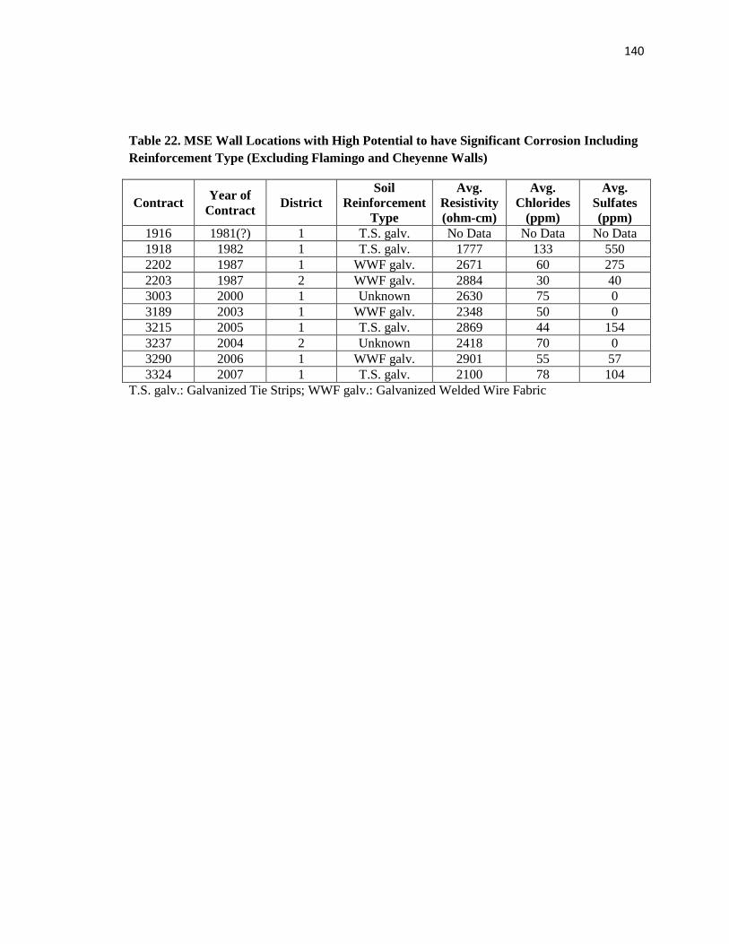
140

Table 22. MSE Wall Locations with High Potential to have Significant Corrosion Including

Reinforcement Type (Excluding Flamingo and Cheyenne Walls)

Contract Year of

Contract District

Soil

Reinforcement

Type

Avg.

Resistivity

(ohm-cm)

Avg.

Chlorides

(ppm)

Avg.

Sulfates

(ppm)

1916 1981(?) 1 T.S. galv. No Data No Data No Data

1918 1982 1 T.S. galv. 1777 133 550

2202 1987 1 WWF galv. 2671 60 275

2203 1987 2 WWF galv. 2884 30 40

3003 2000 1 Unknown 2630 75 0

3189 2003 1 WWF galv. 2348 50 0

3215 2005 1 T.S. galv. 2869 44 154

3237 2004 2 Unknown 2418 70 0

3290 2006 1 WWF galv. 2901 55 57

3324 2007 1 T.S. galv. 2100 78 104

T.S. galv.: Galvanized Tie Strips; WWF galv.: Galvanized Welded Wire Fabric

141

Tab

le 2

3.

Ra

nk

ing

of

Nev

ad

a M

SE

Wall

Can

did

ate

Sit

es f

or

Fu

ture

In

ves

tigati

on

Shad

ed C

ells

do

no

t p

ass.

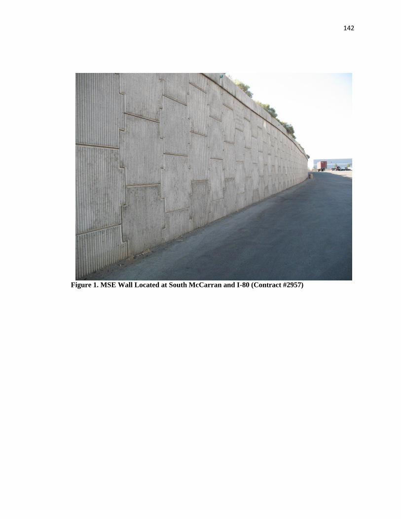
142

Figure 1. MSE Wall Located at South McCarran and I-80 (Contract #2957)

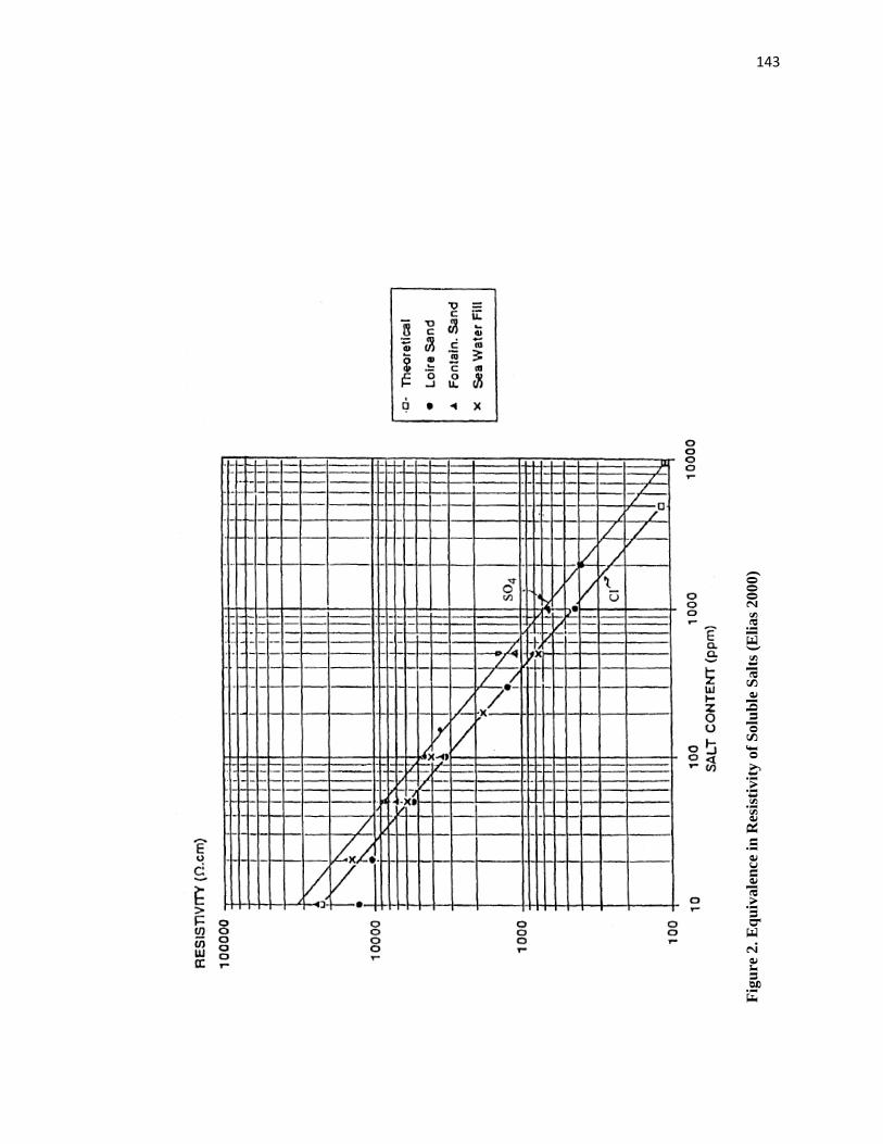
143

Fig

ure

2. E

qu

ivale

nce

in

Res

isti

vit

y o

f S

olu

ble

Salt

s (E

lias

2000)

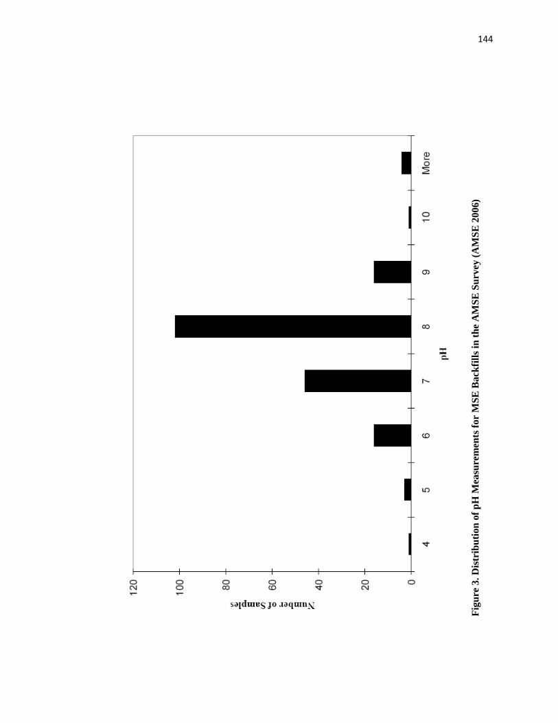
144

Fig

ure

3. D

istr

ibu

tio

n o

f p

H M

easu

rem

ents

for

MS

E B

ack

fill

s in

th

e A

MS

E S

urv

ey (

AM

SE

20

06)

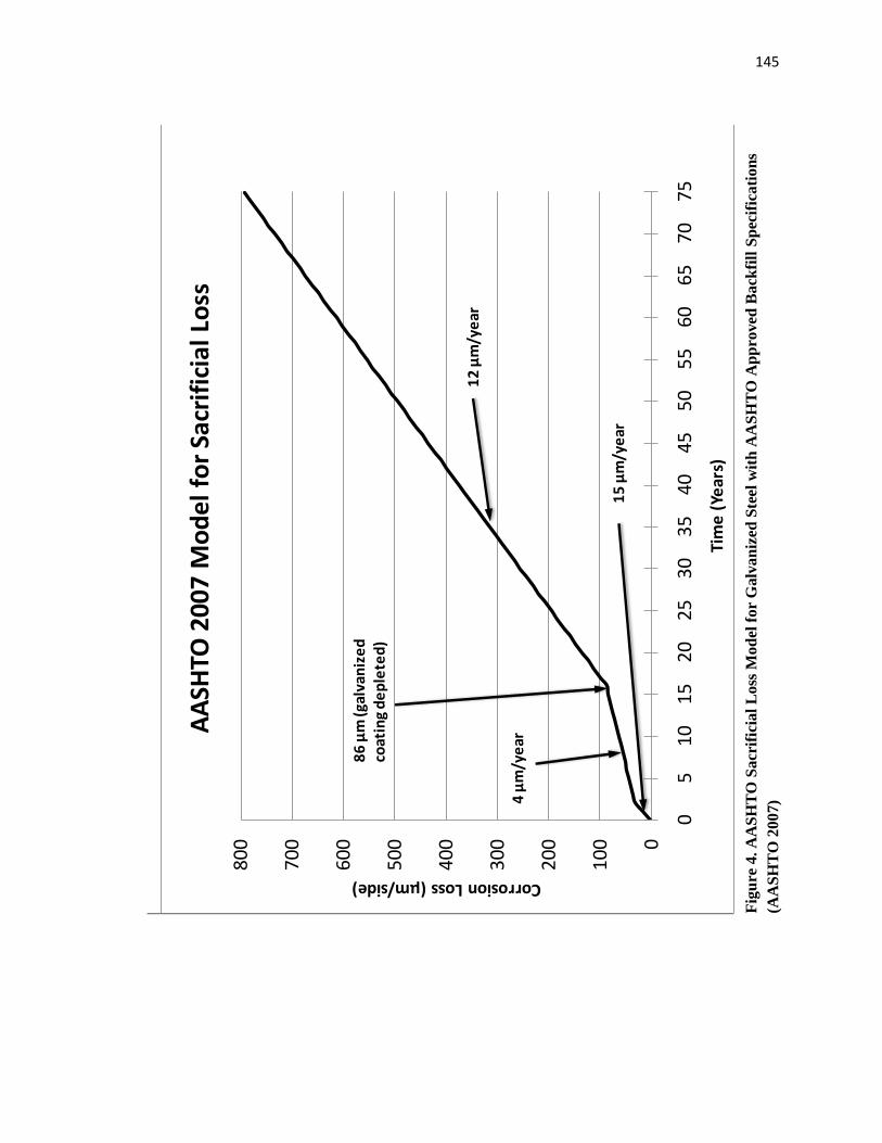
145

Fig

ure

4. A

AS

HT

O S

acr

ific

ial

Loss

Mod

el f

or

Galv

an

ized

Ste

el w

ith

AA

SH

TO

Ap

pro

ved

Ba

ckfi

ll S

pec

ific

ati

on

s

(AA

SH

TO

20

07)

0

10

0

20

0

300

40

0

50

0

60

0

70

0

80

0

05

1015

20

2530

35

4045

50

55

6065

70

75

Corrosion Loss (μm/side)

Tim

e (

Year

s)

AA

SHTO

200

7 M

od

el f

or

Sacr

ific

ial L

oss

12

μm

/ye

ar

86

μm

(gal

van

ize

d

coat

ing

de

ple

ted

)

4 μ

m/y

ear

15

μm

/ye

ar

146

Fig

ure

5. 1

99

0 F

HW

A S

acr

ific

ial

Loss

Mod

el f

or

Bla

ck S

teel

wit

h A

AS

HT

O A

pp

rov

ed B

ack

fill

Sp

ecif

ica

tio

ns

(Eli

as

19

90

)

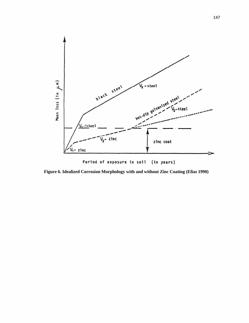
147

Figure 6. Idealized Corrosion Morphology with and without Zinc Coating (Elias 1990)

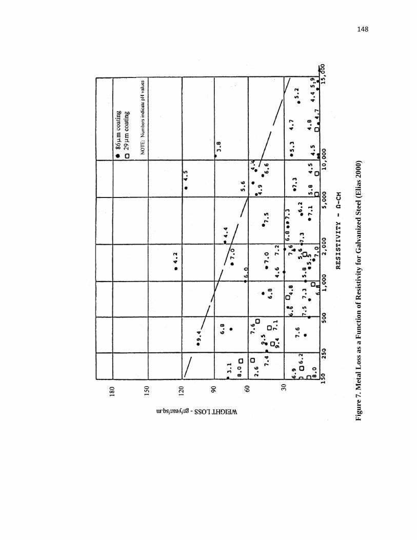
148

Fig

ure

7.

Met

al

Loss

as

a F

un

ctio

n o

f R

esis

tivit

y f

or

Galv

an

ized

Ste

el (

Eli

as

20

00

)

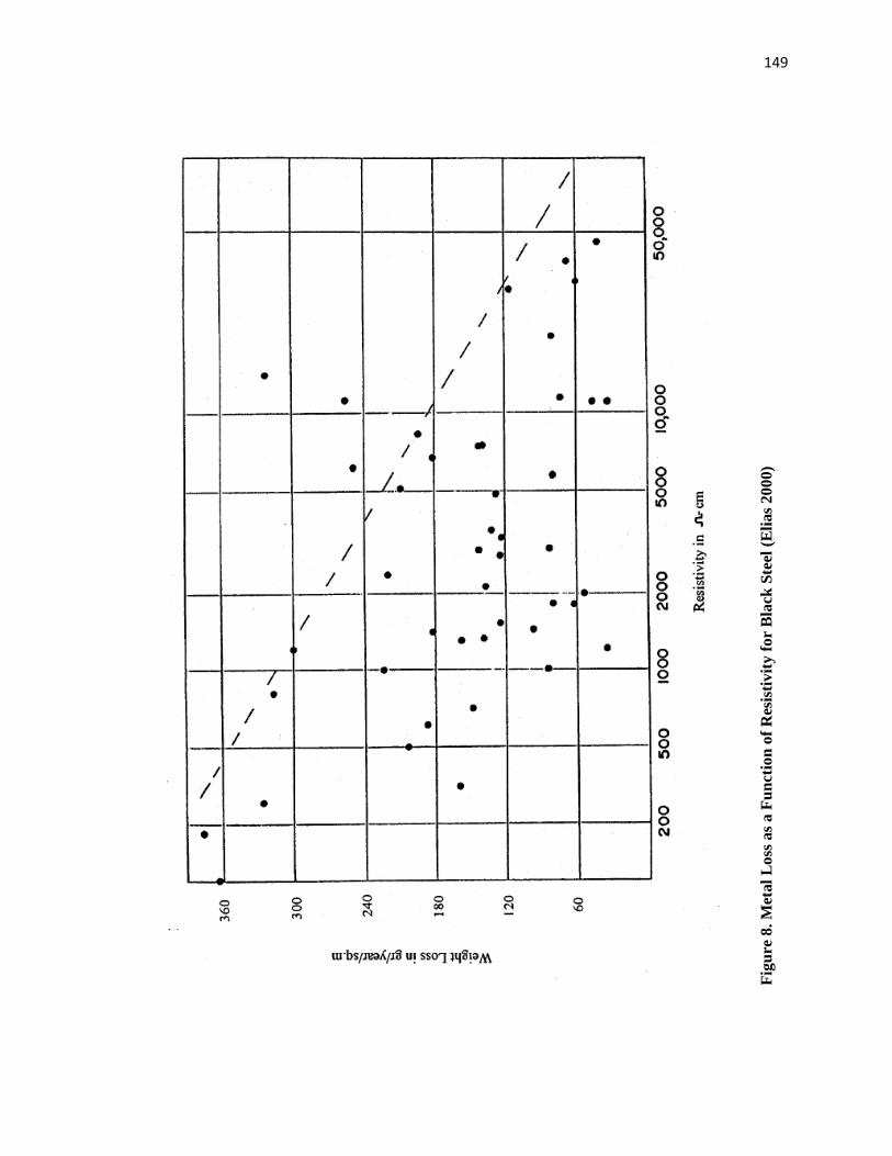
149

Fig

ure

8. M

etal

Lo

ss a

s a

Fu

nct

ion

of

Res

isti

vit

y f

or

Bla

ck S

teel

(E

lias

2000)

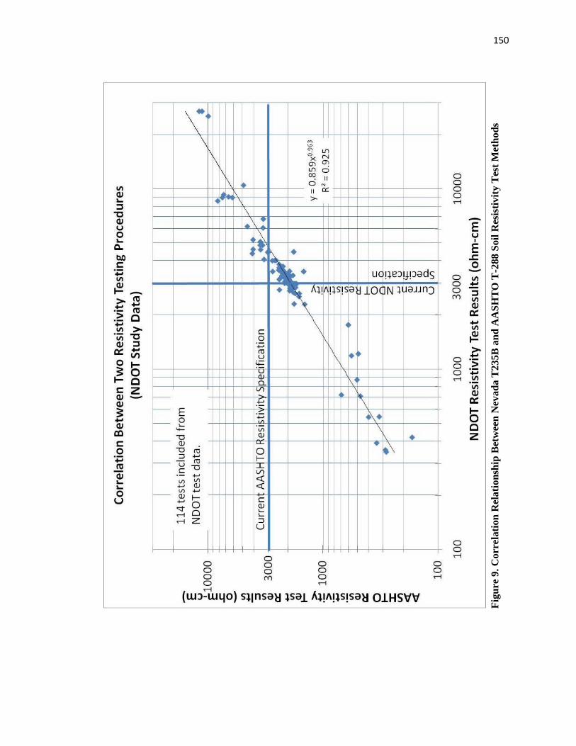
150

Fig

ure

9. C

orr

elati

on

Rel

ati

on

ship

Bet

wee

n N

evad

a T

235B

an

d A

AS

HT

O T

-288

Soil

Res

isti

vit

y T

est

Met

ho

ds

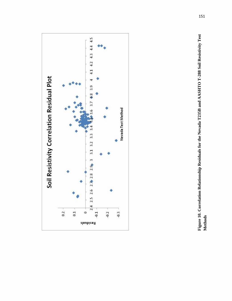
151

Fig

ure

10

. C

orr

elati

on

Rel

ati

on

ship

Res

idu

als

for

the

Nev

ad

a T

235B

an

d A

AS

HT

O T

-28

8 S

oil

Res

isti

vit

y T

est

Met

ho

ds

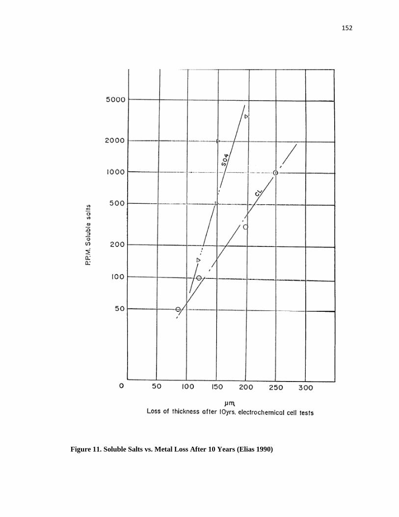
152

Figure 11. Soluble Salts vs. Metal Loss After 10 Years (Elias 1990)

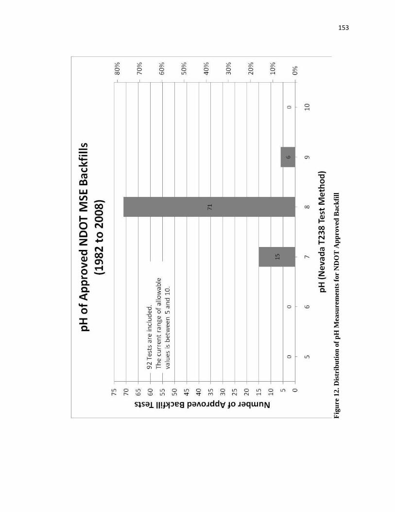
153

Fig

ure

12

. D

istr

ibu

tio

n o

f p

H M

easu

rem

ents

for

ND

OT

Ap

pro

ved

Back

fill

154

Fig

ure

13

. p

H v

s. R

esis

tivit

y M

easu

rem

ents

for

ND

OT

Ap

pro

ved

Back

fill

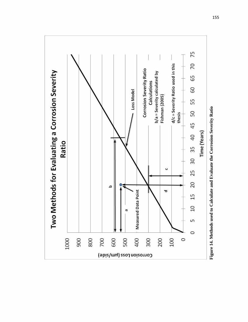
155

Fig

ure

14

. M

eth

od

s u

sed

to C

alc

ula

te a

nd

Evalu

ate

th

e C

orr

osi

on

Sev

erit

y R

ati

o

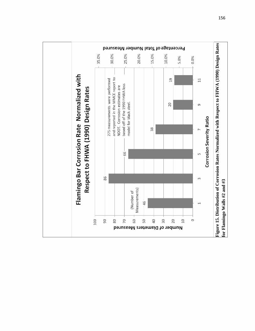
156

Fig

ure

15.

Dis

trib

uti

on

of

Corr

osi

on

Rate

s N

orm

ali

zed

wit

h R

esp

ect

to F

HW

A (

19

90

) D

esig

n R

ate

s

for

Fla

min

go W

all

s #2 a

nd

#3

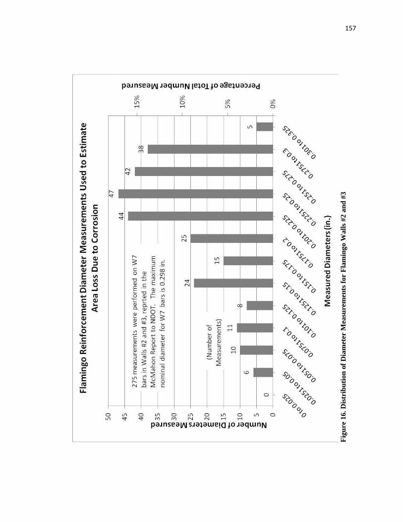
157

Fig

ure

16

. D

istr

ibu

tio

n o

f D

iam

eter

Mea

sure

men

ts f

or

Fla

min

go W

all

s #2 a

nd

#3

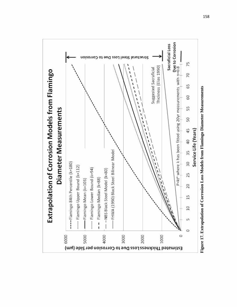
158

Fig

ure

17

. E

xtr

ap

ola

tio

n o

f C

orr

osi

on

Loss

Mod

els

from

Fla

min

go D

iam

eter

Mea

sure

men

ts

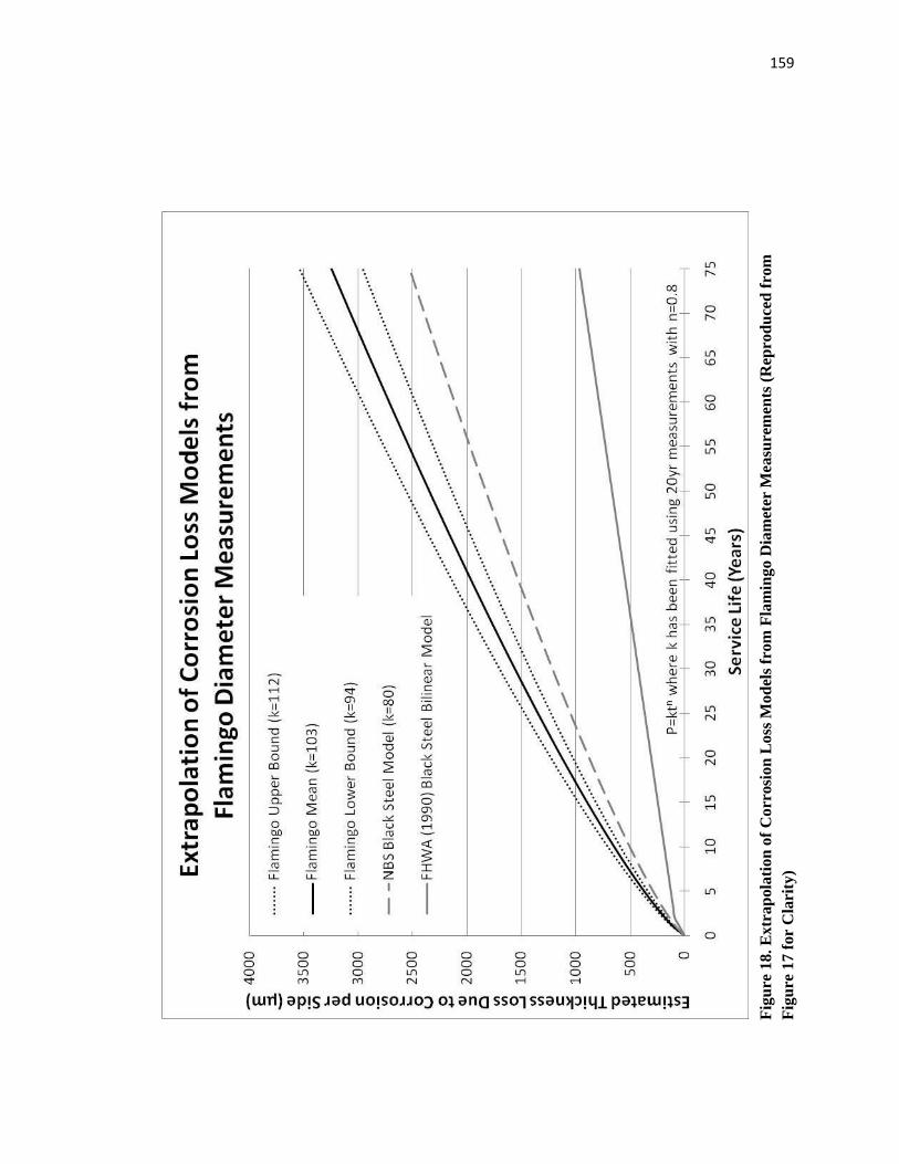
159

Fig

ure

18

. E

xtr

ap

ola

tio

n o

f C

orr

osi

on

Loss

Mod

els

from

Fla

min

go D

iam

eter

Mea

sure

men

ts (

Rep

rod

uce

d f

rom

Fig

ure

17

for

Cla

rity

)

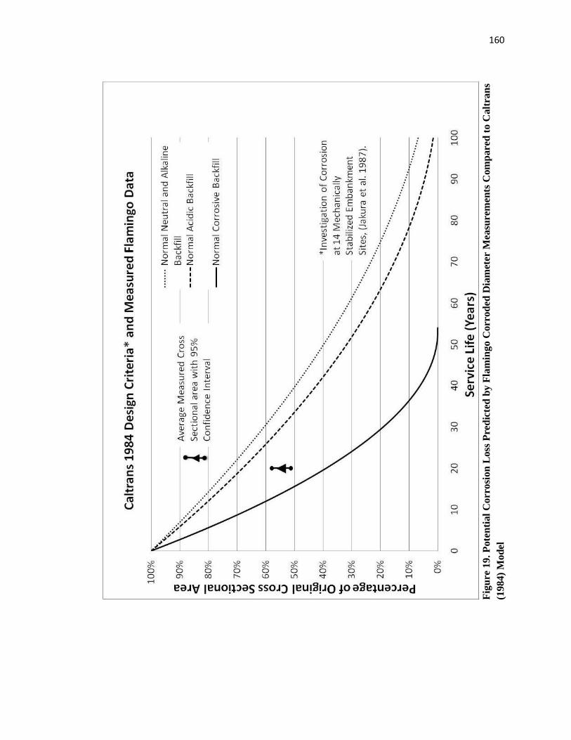
160

Fig

ure

19

. P

ote

nti

al

Corr

osi

on

Loss

Pre

dic

ted

by F

lam

ingo C

orr

od

ed D

iam

eter

Mea

sure

men

ts C

om

pare

d t

o C

alt

ran

s

(19

84)

Mo

del

161

Fig

ure

20

. R

an

ges

of

Ori

gin

al

Fla

min

go M

easu

red

Res

isti

vit

y V

alu

es (

by L

ab

ora

tory

)

162

Fig

ure

21

. O

rig

inal

Fla

min

go M

easu

red

Res

isti

vit

y L

SD

An

aly

sis

Res

ult

s

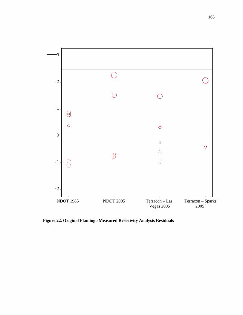
163

Figure 22. Original Flamingo Measured Resistivity Analysis Residuals

Stu

de

nt

Re

sid

ua

l

-2

-1

0

1

2

3

testgroup

NPT_85 NT_2005 T_LV T_Sparks NDOT 1985 NDOT 2005 Terracon – Las Terracon – Sparks

Vegas 2005 2005

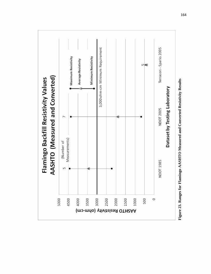
164

Fig

ure

23

. R

an

ges

for

Fla

min

go A

AS

HT

O M

easu

red

an

d C

on

ver

ted

Res

isti

vit

y R

esu

lts

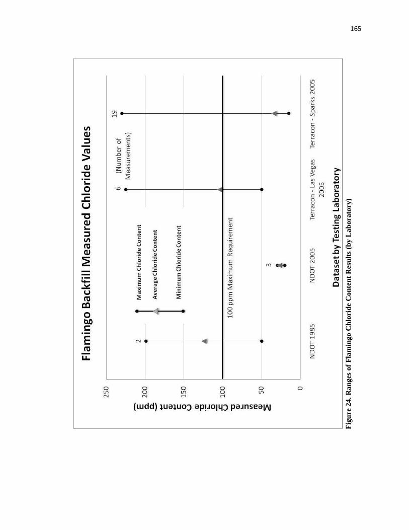
165

Fig

ure

24

. R

an

ges

of

Fla

min

go C

hlo

rid

e C

on

ten

t R

esu

lts

(by L

ab

ora

tory

)

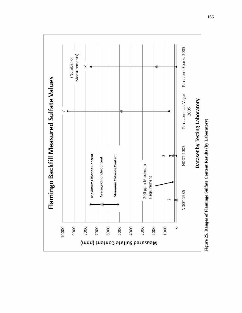
166

Fig

ure

25

. R

an

ges

of

Fla

min

go S

ulf

ate

Con

ten

t R

esu

lts

(by L

ab

ora

tory

)

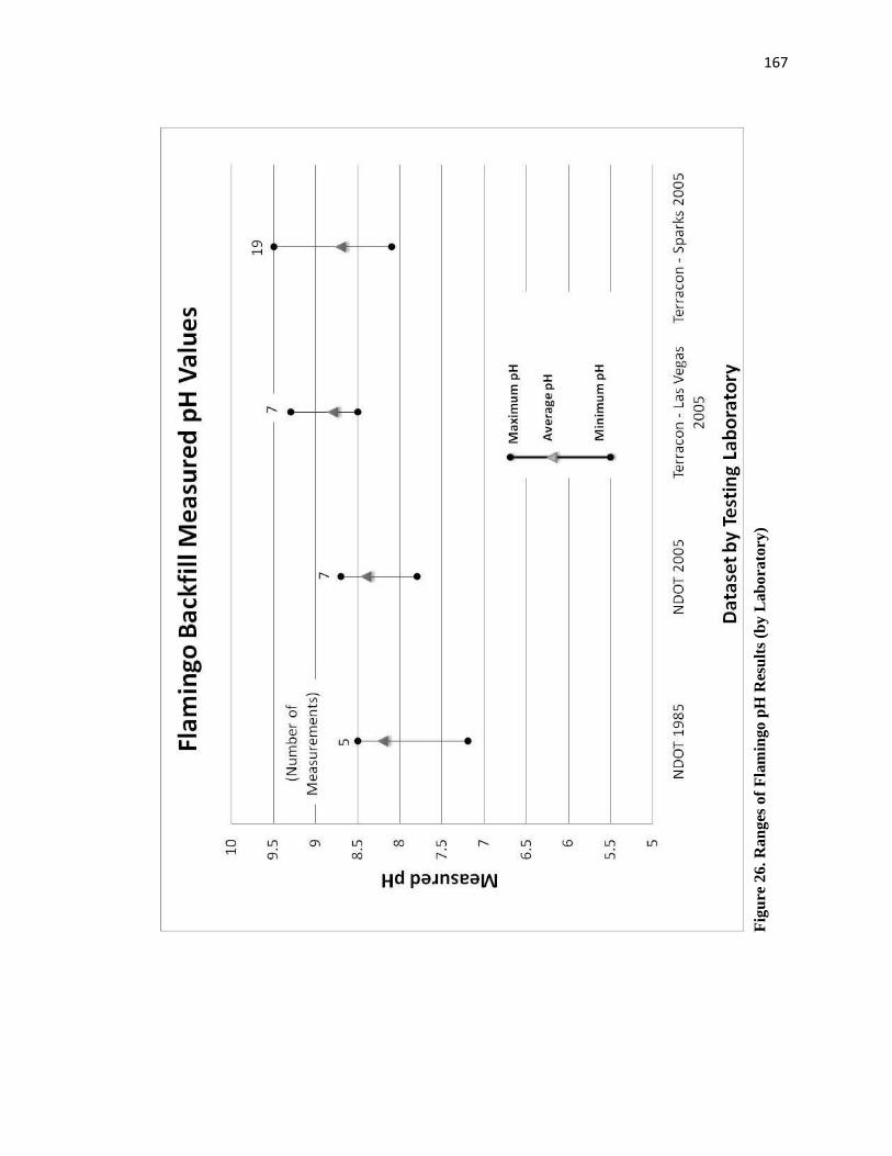
167

Fig

ure

26

. R

an

ges

of

Fla

min

go p

H R

esu

lts

(by L

ab

ora

tory

)

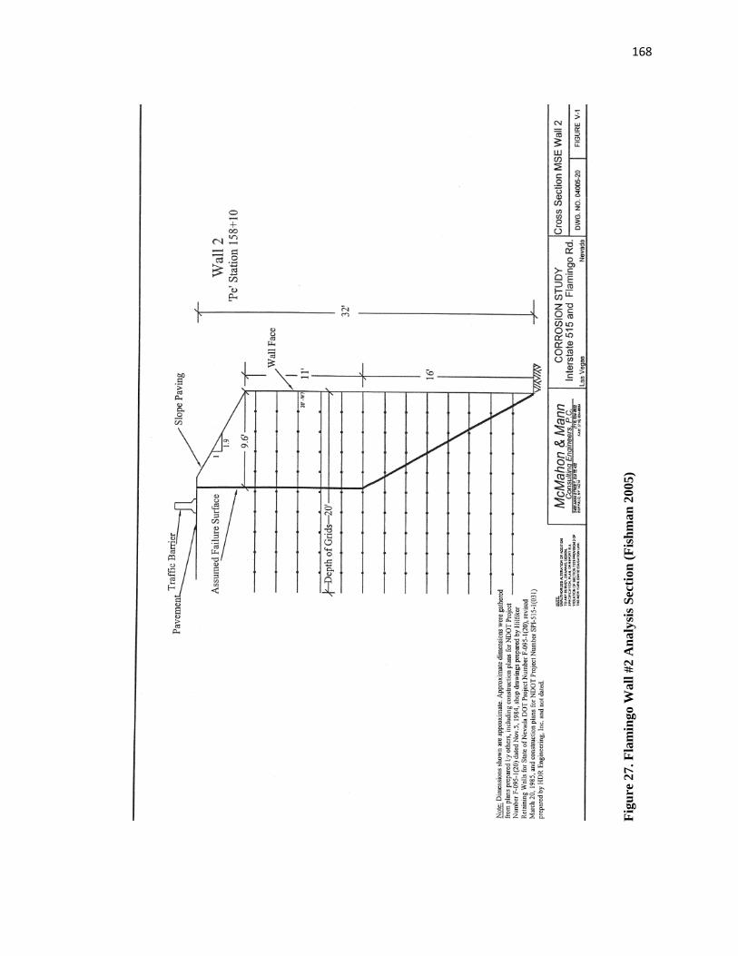
168

Fig

ure

27

. F

lam

ing

o W

all

#2

An

aly

sis

Sec

tion

(F

ish

man

2005)

169

Fig

ure

28

. F

lam

ing

o W

all

#3

An

aly

sis

Sec

tion

(F

ish

man

2005)

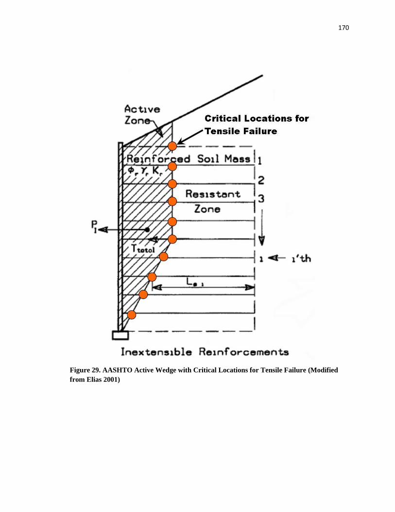
170

Figure 29. AASHTO Active Wedge with Critical Locations for Tensile Failure (Modified

from Elias 2001)

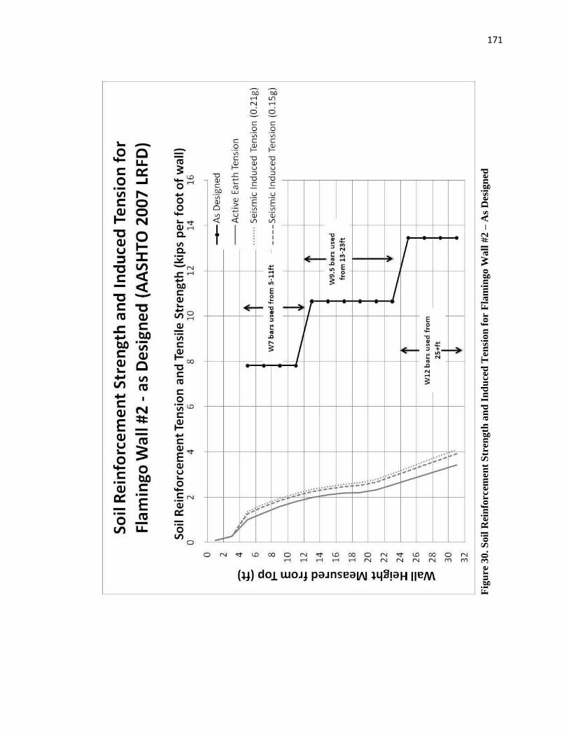
171

Fig

ure

30.

Soil

Rei

nfo

rcem

ent

Str

ength

an

d I

nd

uce

d T

ensi

on

for

Fla

min

go W

all

#2

– A

s D

esig

ned

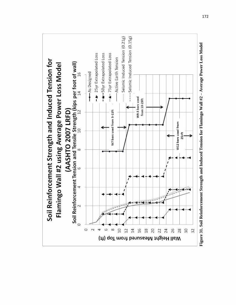
172

Fig

ure

31.

Soil

Rei

nfo

rcem

ent

Str

ength

an

d I

nd

uce

d T

ensi

on

for

Fla

min

go W

all

#2

– A

ver

age

Po

wer

Lo

ss M

od

el

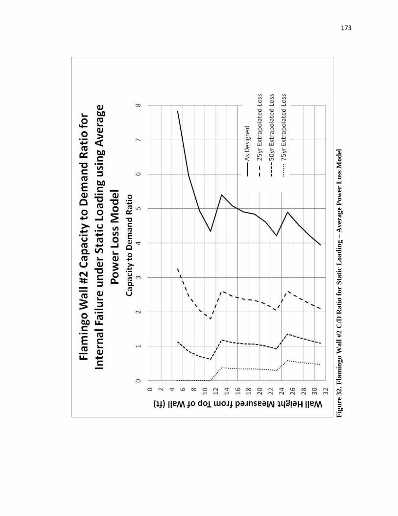
173

Fig

ure

32

. F

lam

ing

o W

all

#2 C

/D R

ati

o f

or

Sta

tic

Load

ing –

Aver

age

Pow

er L

oss

Mo

del

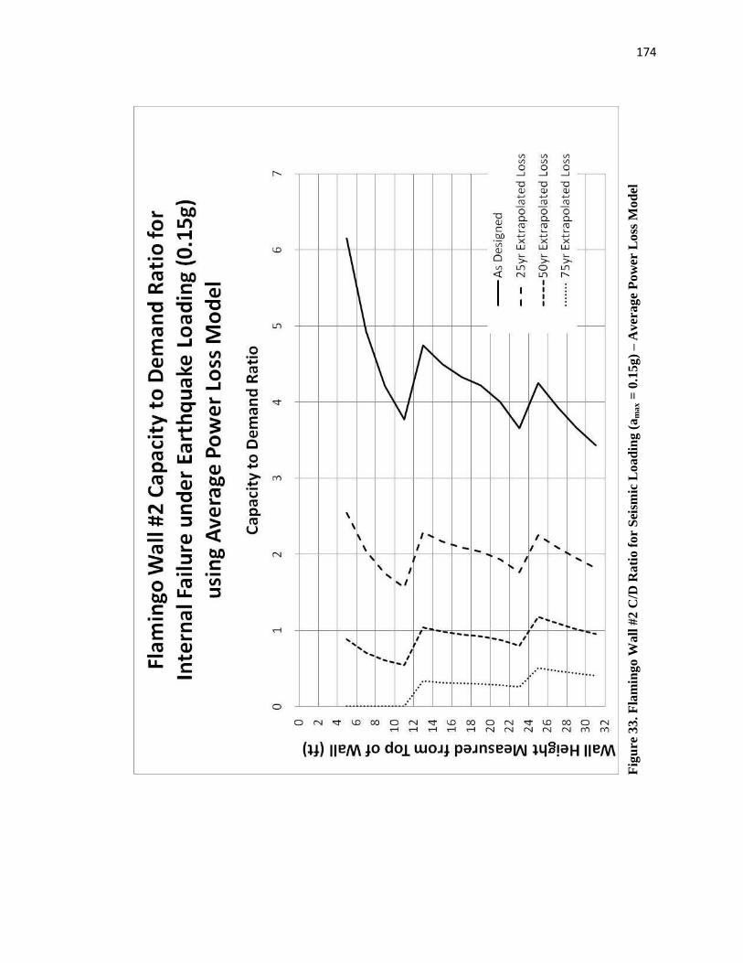
174

Fig

ure

33

. F

lam

ing

o W

all

#2 C

/D R

ati

o f

or

Sei

smic

Load

ing (

am

ax =

0.1

5g)

– A

ver

ag

e P

ow

er L

oss

Mo

del

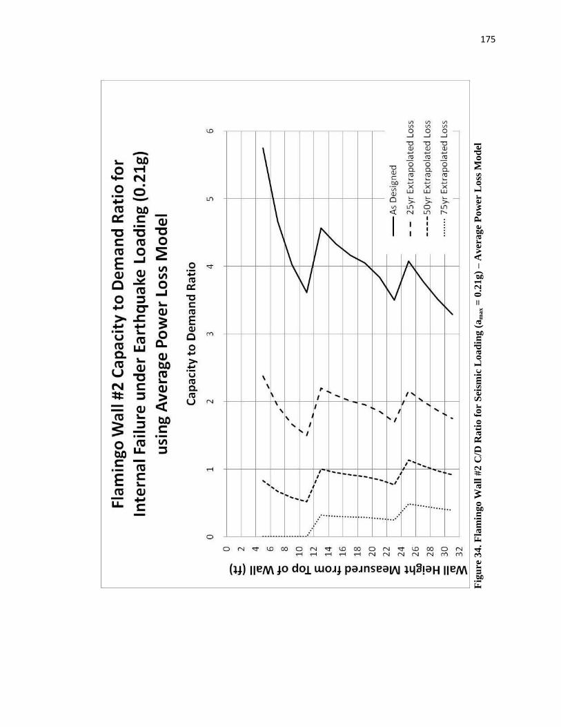
175

Fig

ure

34

. F

lam

ing

o W

all

#2 C

/D R

ati

o f

or

Sei

smic

Load

ing (

am

ax =

0.2

1g)

– A

ver

ag

e P

ow

er L

oss

Mo

del

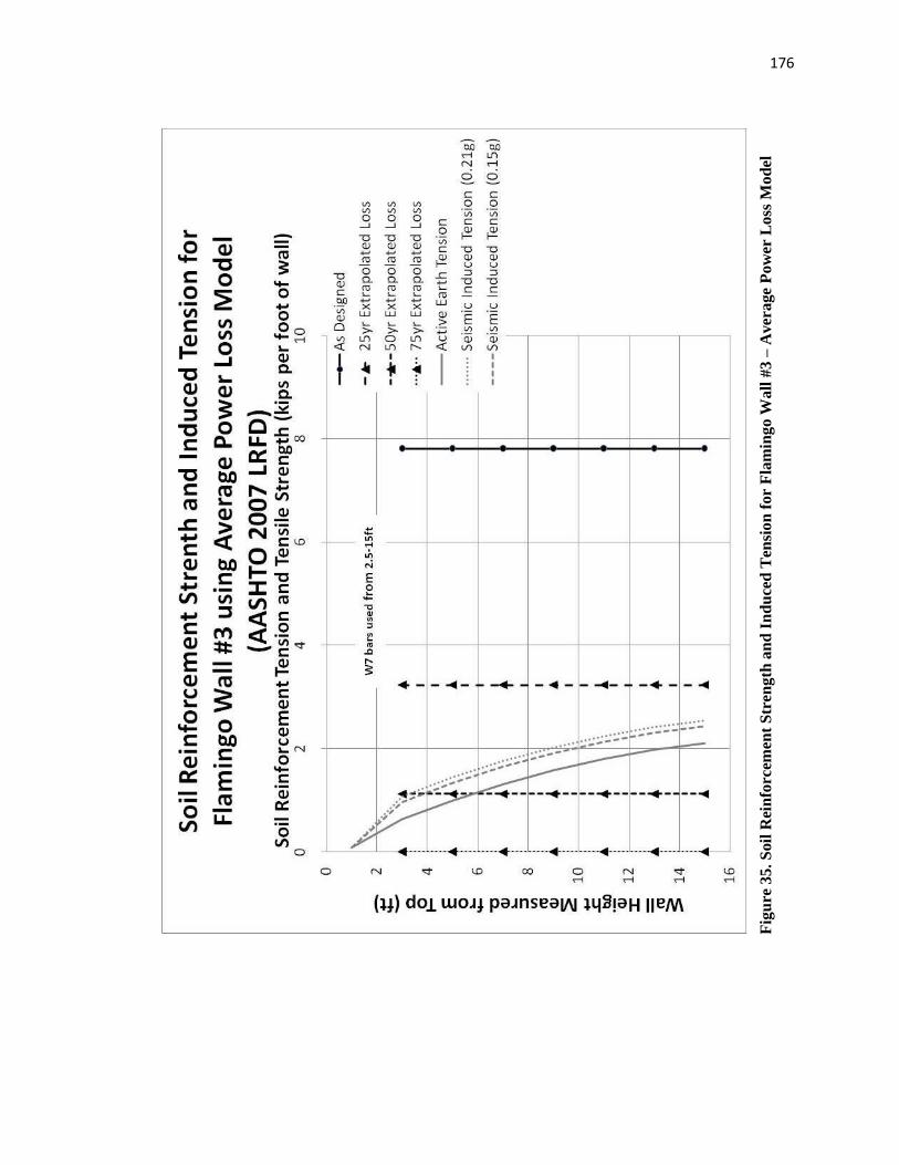
176

Fig

ure

35.

Soil

Rei

nfo

rcem

ent

Str

ength

an

d I

nd

uce

d T

ensi

on

for

Fla

min

go W

all

#3

– A

ver

age

Po

wer

Lo

ss M

od

el

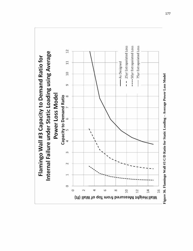
177

Fig

ure

36

. F

lam

ing

o W

all

#3 C

/D R

ati

o f

or

Sta

tic

Load

ing –

Aver

age

Pow

er L

oss

Mo

del

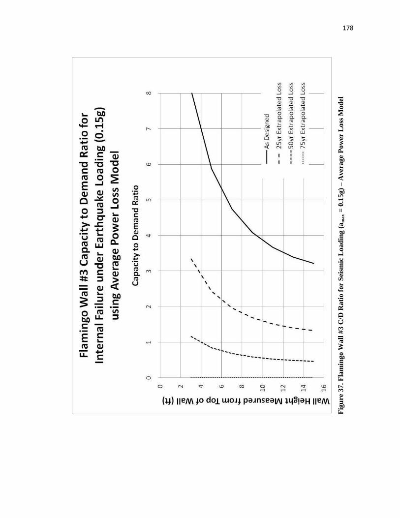
178

Fig

ure

37

. F

lam

ing

o W

all

#3 C

/D R

ati

o f

or

Sei

smic

Load

ing (

am

ax =

0.1

5g)

– A

ver

ag

e P

ow

er L

oss

Mo

del

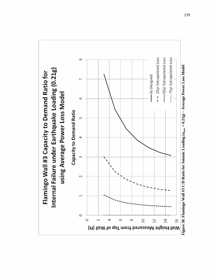
179

Fig

ure

38

. F

lam

ing

o W

all

#3

C/D

Rati

o f

or

Sei

smic

Load

ing (

am

ax =

0.2

1g)

– A

ver

age

Po

wer

Lo

ss M

od

el

180

Fig

ure

39.

Soil

Rei

nfo

rcem

ent

Str

ength

an

d I

nd

uce

d T

ensi

on

for

Fla

min

go W

all

#2 –

84

th P

erce

nti

le P

ow

er L

oss

Mod

el

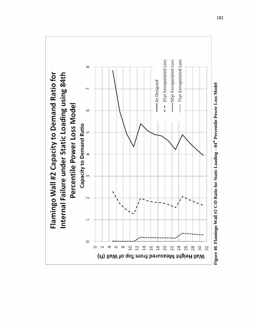
181

Fig

ure

40. F

lam

ing

o W

all

#2 C

/D R

ati

o f

or

Sta

tic

Load

ing –

84

th P

erce

nti

le P

ow

er L

oss

Mo

del

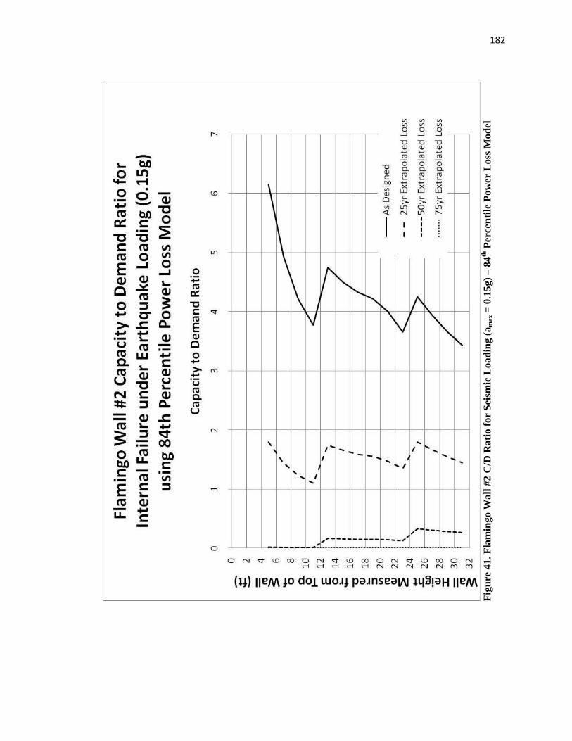
182

Fig

ure

41. F

lam

ing

o W

all

#2 C

/D R

ati

o f

or

Sei

smic

Load

ing (

am

ax =

0.1

5g)

– 8

4th

Per

cen

tile

Po

wer

Loss

Mo

del

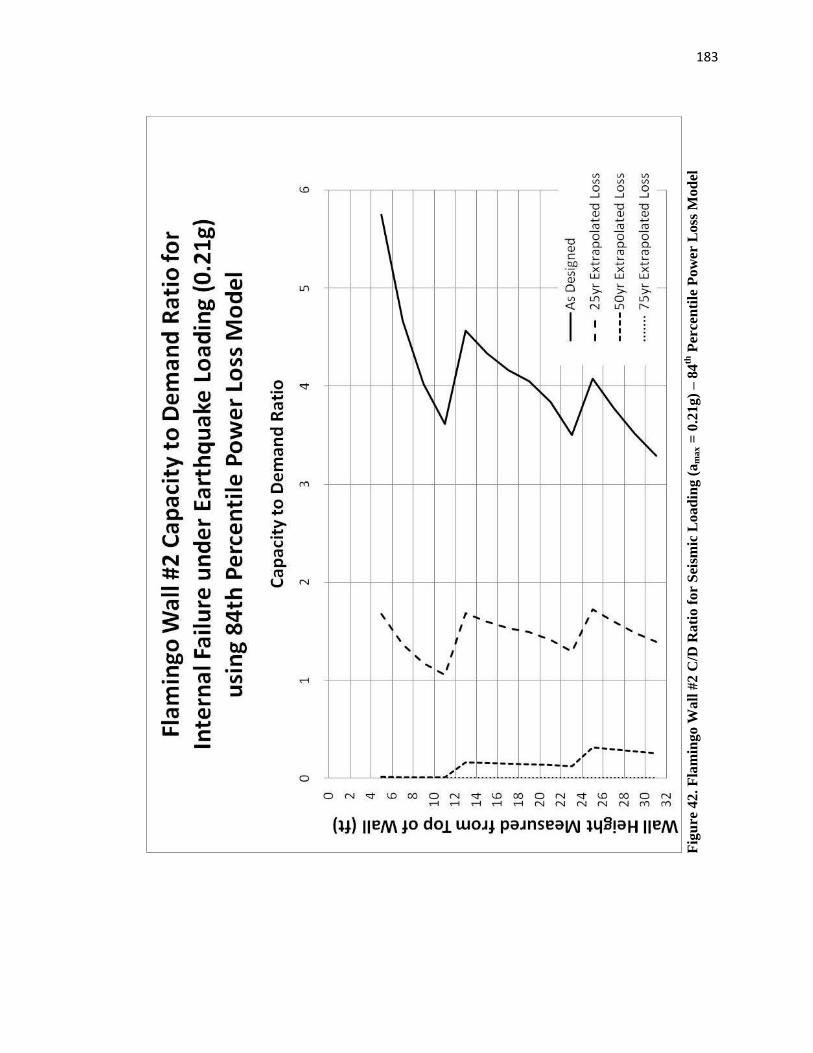
183

Fig

ure

42.

Fla

min

go

Wall

#2 C

/D R

ati

o f

or

Sei

smic

Load

ing (

am

ax =

0.2

1g)

– 8

4th

Per

cen

tile

Po

wer

Loss

Mo

del

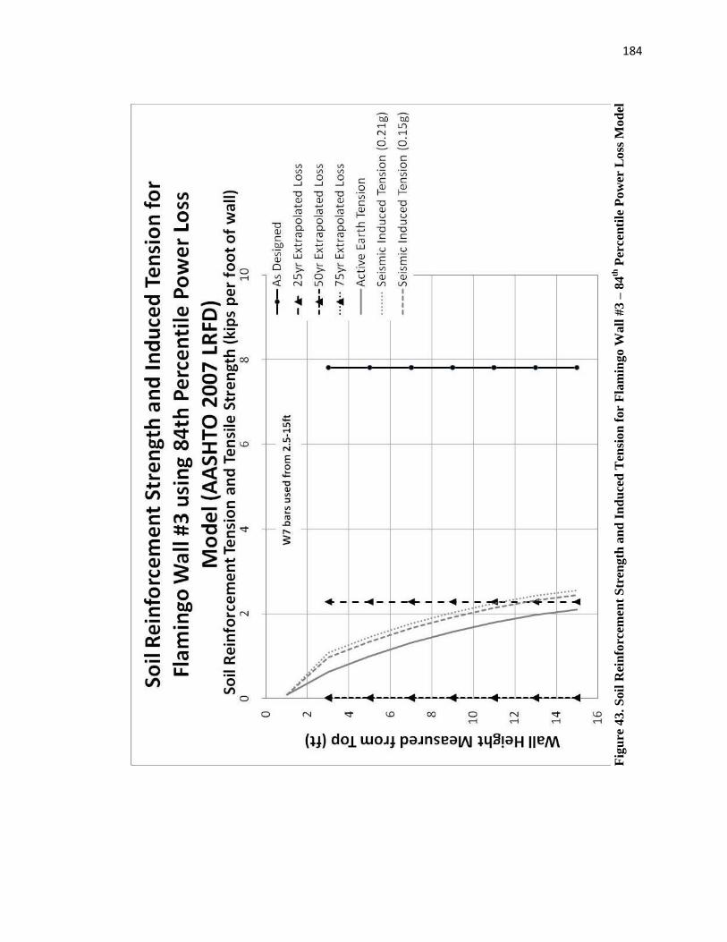
184

Fig

ure

43

. S

oil

Rei

nfo

rcem

ent

Str

ength

an

d I

nd

uce

d T

ensi

on

for

Fla

min

go W

all

#3

– 8

4th

Per

cen

tile

Po

wer

Lo

ss M

od

el

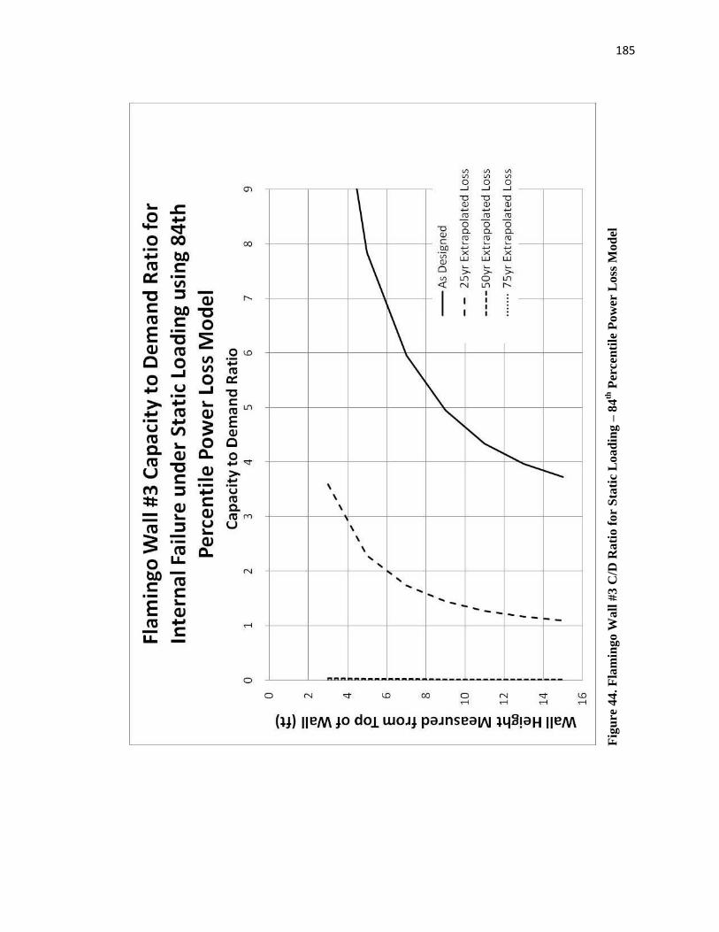
185

Fig

ure

44

. F

lam

ing

o W

all

#3 C

/D R

ati

o f

or

Sta

tic

Load

ing –

84

th P

erce

nti

le P

ow

er L

oss

Mo

del

186

Fig

ure

45. F

lam

ing

o W

all

#3 C

/D R

ati

o f

or

Sei

smic

Load

ing (

am

ax =

0.1

5g)

– 8

4th

Per

cen

tile

Po

wer

Loss

Mo

del

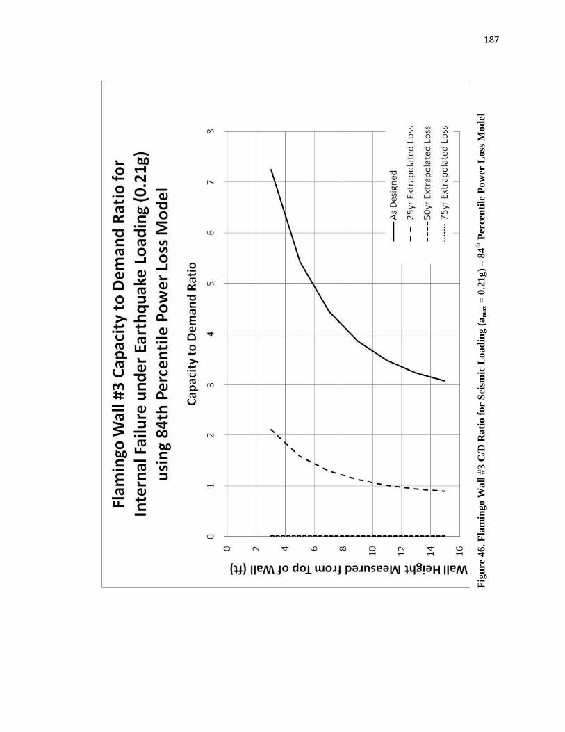
187

Fig

ure

46

. F

lam

ing

o W

all

#3 C

/D R

ati

o f

or

Sei

smic

Load

ing (

am

ax =

0.2

1g)

– 8

4th

Per

cen

tile

Po

wer

Loss

Mo

del

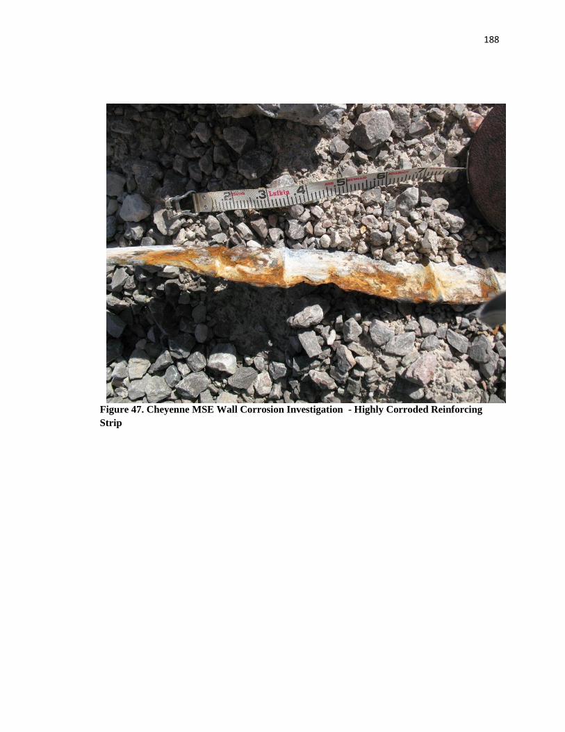
188

Figure 47. Cheyenne MSE Wall Corrosion Investigation - Highly Corroded Reinforcing

Strip

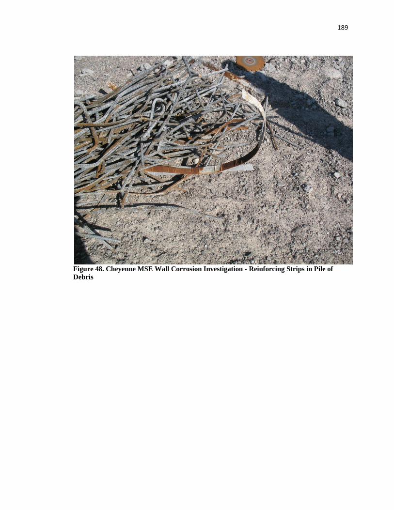
189

Figure 48. Cheyenne MSE Wall Corrosion Investigation - Reinforcing Strips in Pile of

Debris

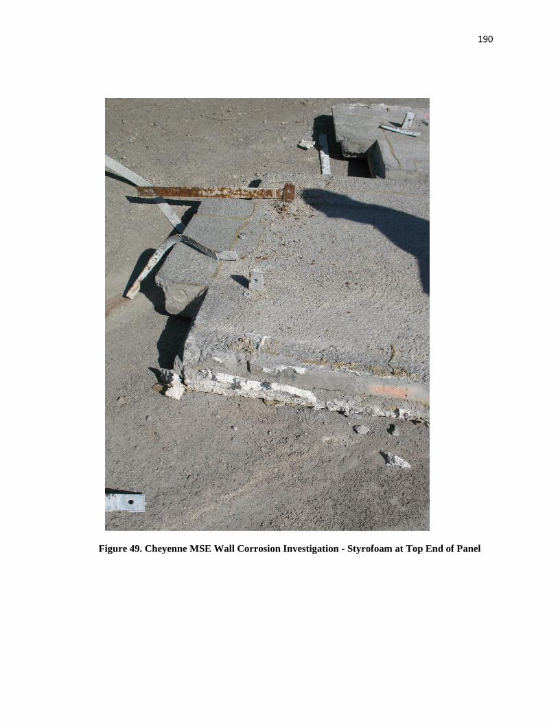
190

Figure 49. Cheyenne MSE Wall Corrosion Investigation - Styrofoam at Top End of Panel

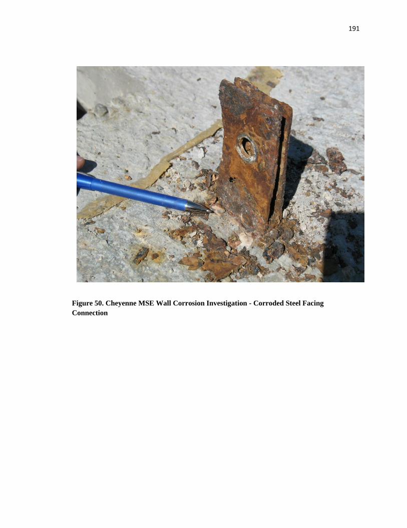
191

Figure 50. Cheyenne MSE Wall Corrosion Investigation - Corroded Steel Facing

Connection

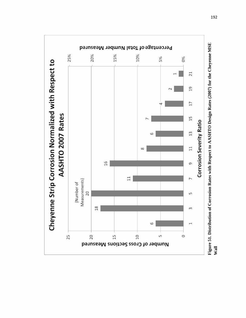
192

Fig

ure

51. D

istr

ibu

tio

n o

f C

orr

osi

on

Rate

s w

ith

Res

pec

t to

AA

SH

TO

Des

ign

Ra

tes

(20

07)

for

the

Ch

eyen

ne

MS

E

Wa

ll

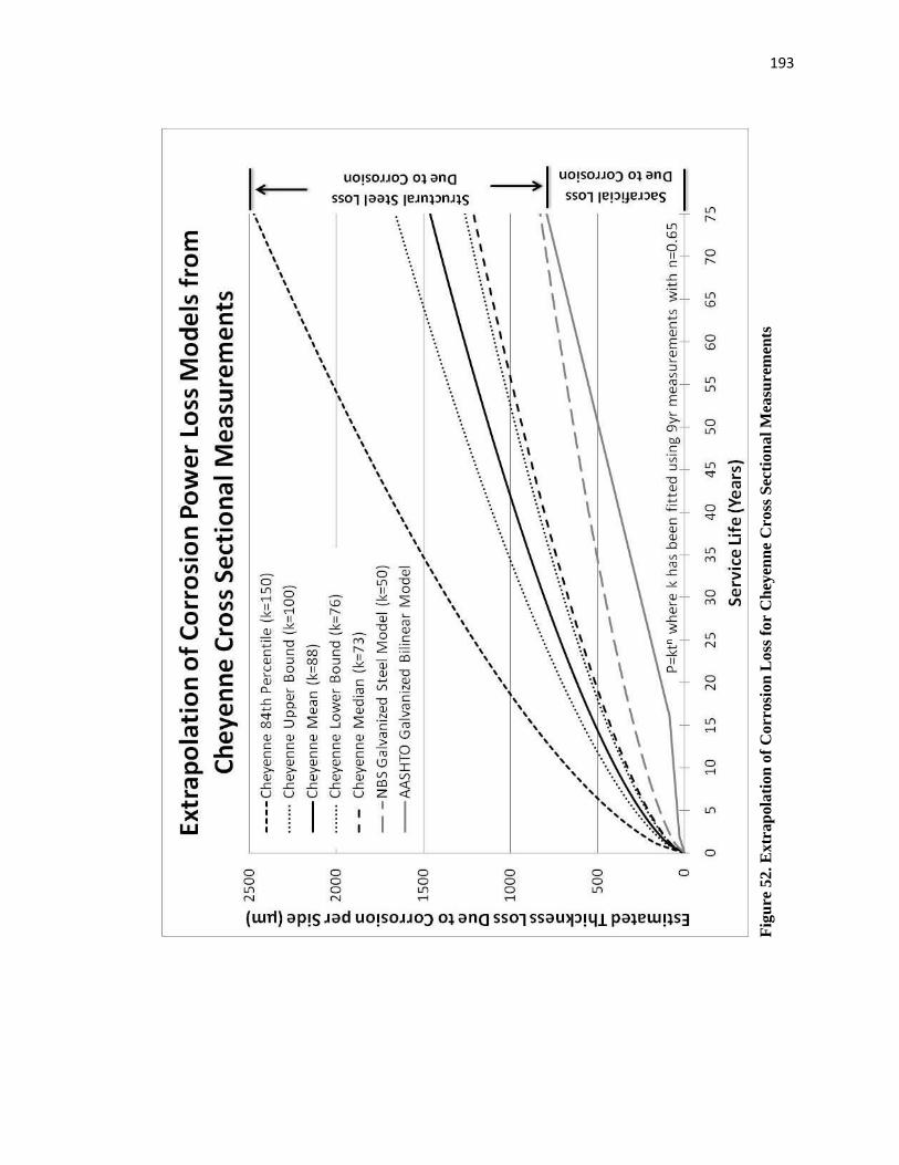
193

Fig

ure

52

. E

xtr

ap

ola

tion

of

Corr

osi

on

Loss

for

Ch

eyen

ne

Cro

ss S

ecti

on

al

Mea

sure

men

ts

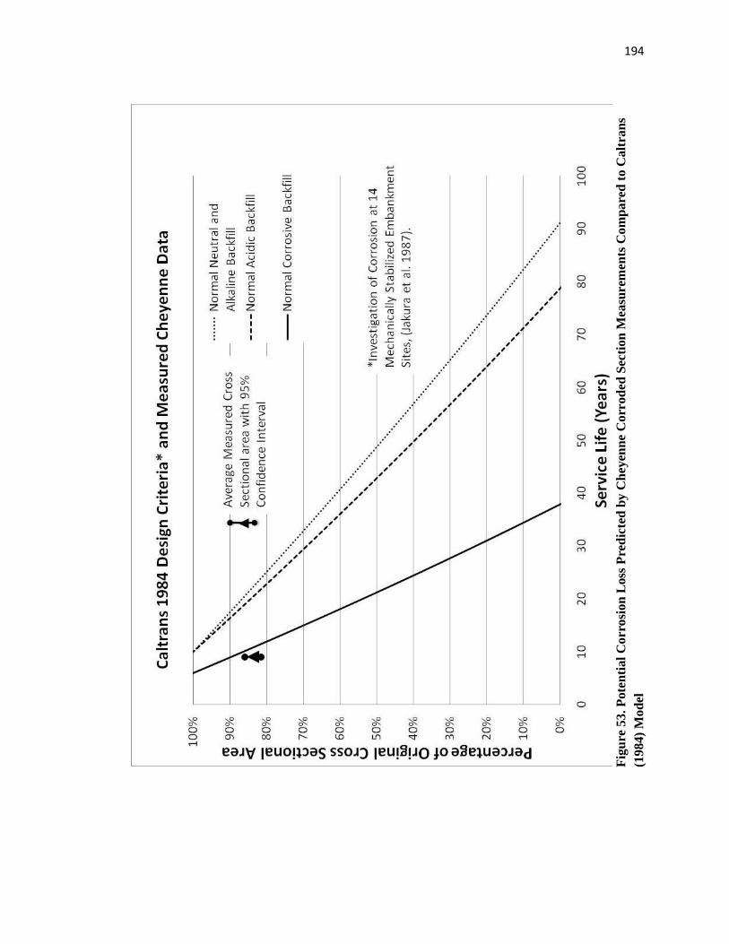
194

Fig

ure

53

. P

ote

nti

al

Co

rrosi

on

Loss

Pre

dic

ted

by C

hey

enn

e C

orr

od

ed S

ecti

on

Mea

sure

men

ts C

om

pa

red

to

Calt

ran

s

(19

84)

Mo

del

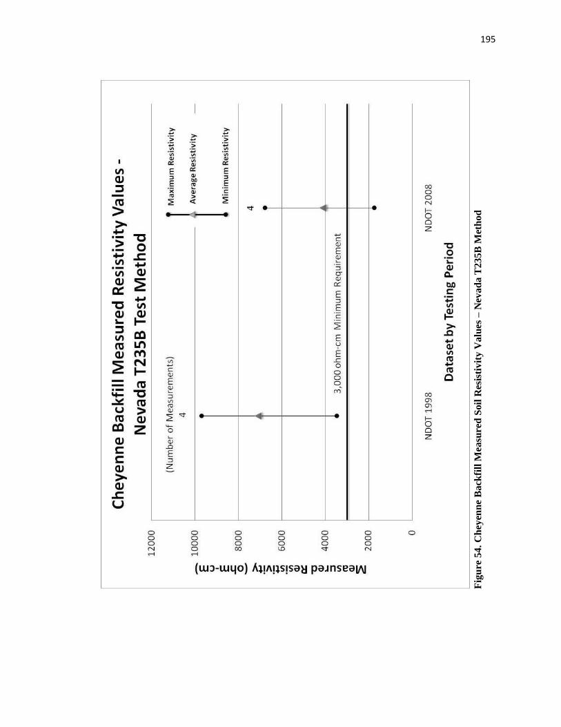
195

Fig

ure

54.

Ch

eyen

ne

Back

fill

Mea

sure

d S

oil

Res

isti

vit

y V

alu

es –

Nev

ad

a T

235

B M

eth

od

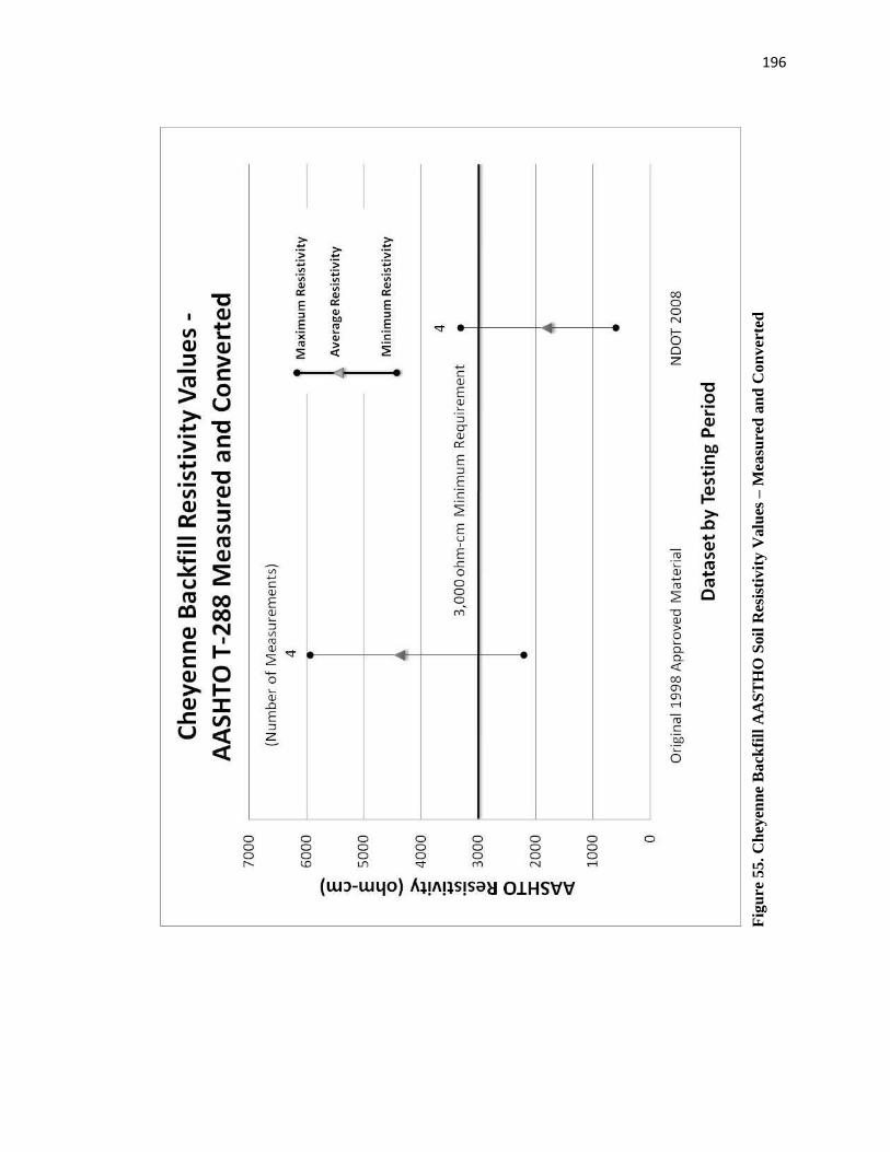
196

Fig

ure

55. C

hey

enn

e B

ack

fill

AA

ST

HO

Soil

Res

isti

vit

y V

alu

es –

Mea

sure

d a

nd

Co

nv

erte

d

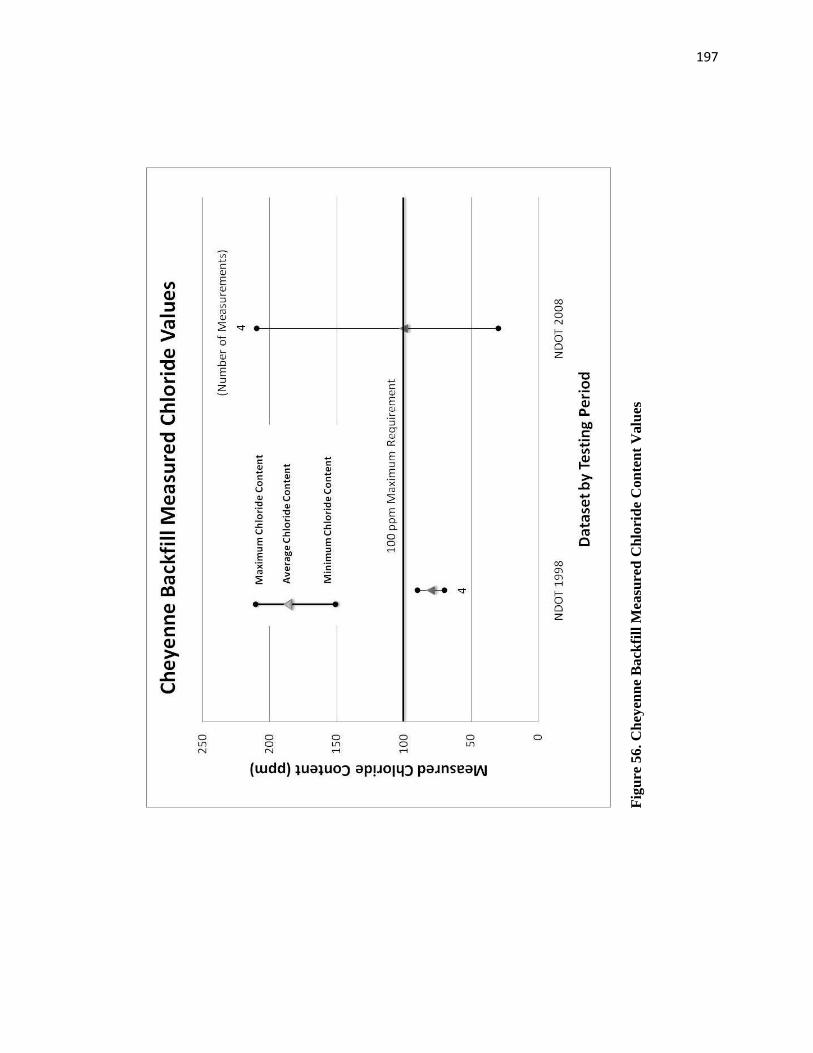
197

Fig

ure

56

. C

hey

enn

e B

ack

fill

Mea

sure

d C

hlo

rid

e C

on

ten

t V

alu

es

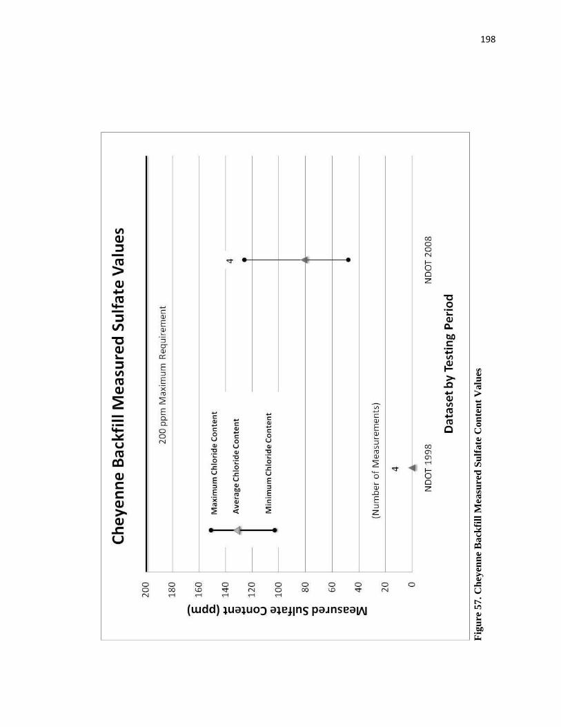
198

Fig

ure

57

. C

hey

enn

e B

ack

fill

Mea

sure

d S

ulf

ate

Con

ten

t V

alu

es

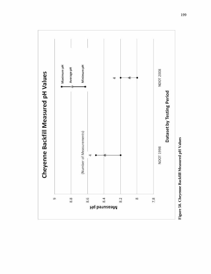
199

Fig

ure

58

. C

hey

enn

e B

ack

fill

Mea

sure

d p

H V

alu

es

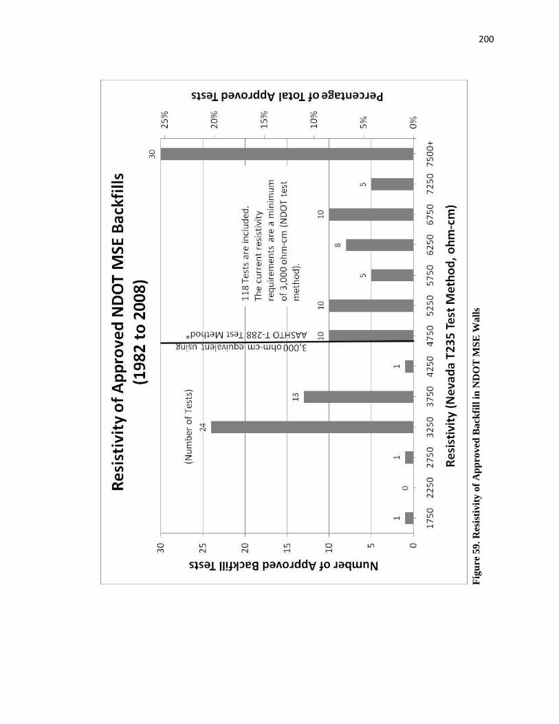
200

Fig

ure

59

. R

esis

tivit

y o

f A

pp

roved

Back

fill

in

ND

OT

MS

E W

all

s

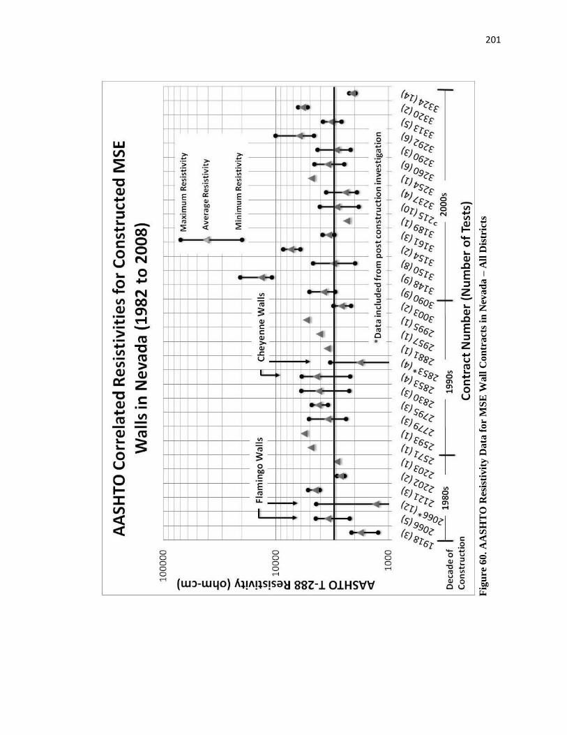
201

Fig

ure

60

. A

AS

HT

O R

esis

tivit

y D

ata

for

MS

E W

all

Con

tract

s in

Nev

ad

a –

All

Dis

tric

ts

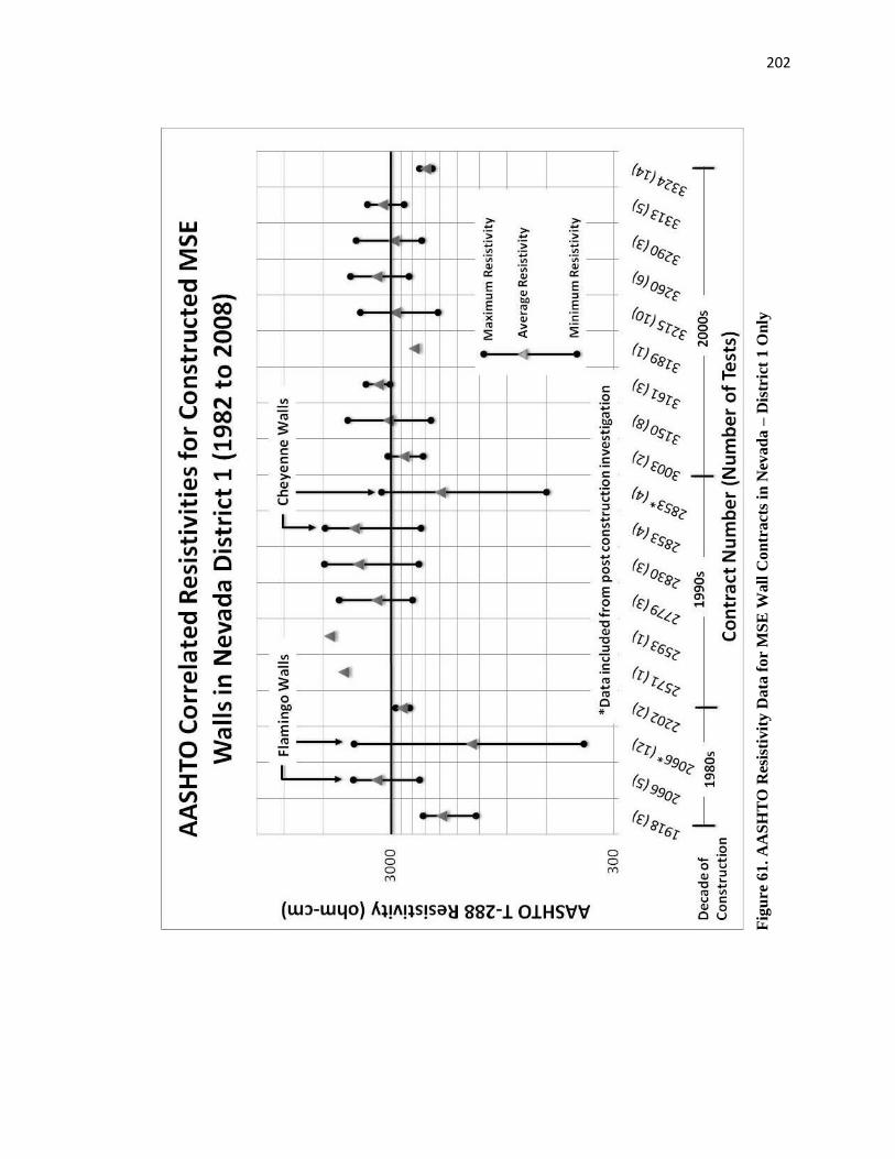
202

Fig

ure

61

. A

AS

HT

O R

esis

tivit

y D

ata

for

MS

E W

all

Con

tract

s in

Nev

ad

a –

Dis

tric

t 1

On

ly

203

Fig

ure

62

. A

AS

HT

O R

esis

tivit

y D

ata

for

MS

E W

all

Con

tract

s in

Nev

ad

a –

Dis

tric

t 2

On

ly

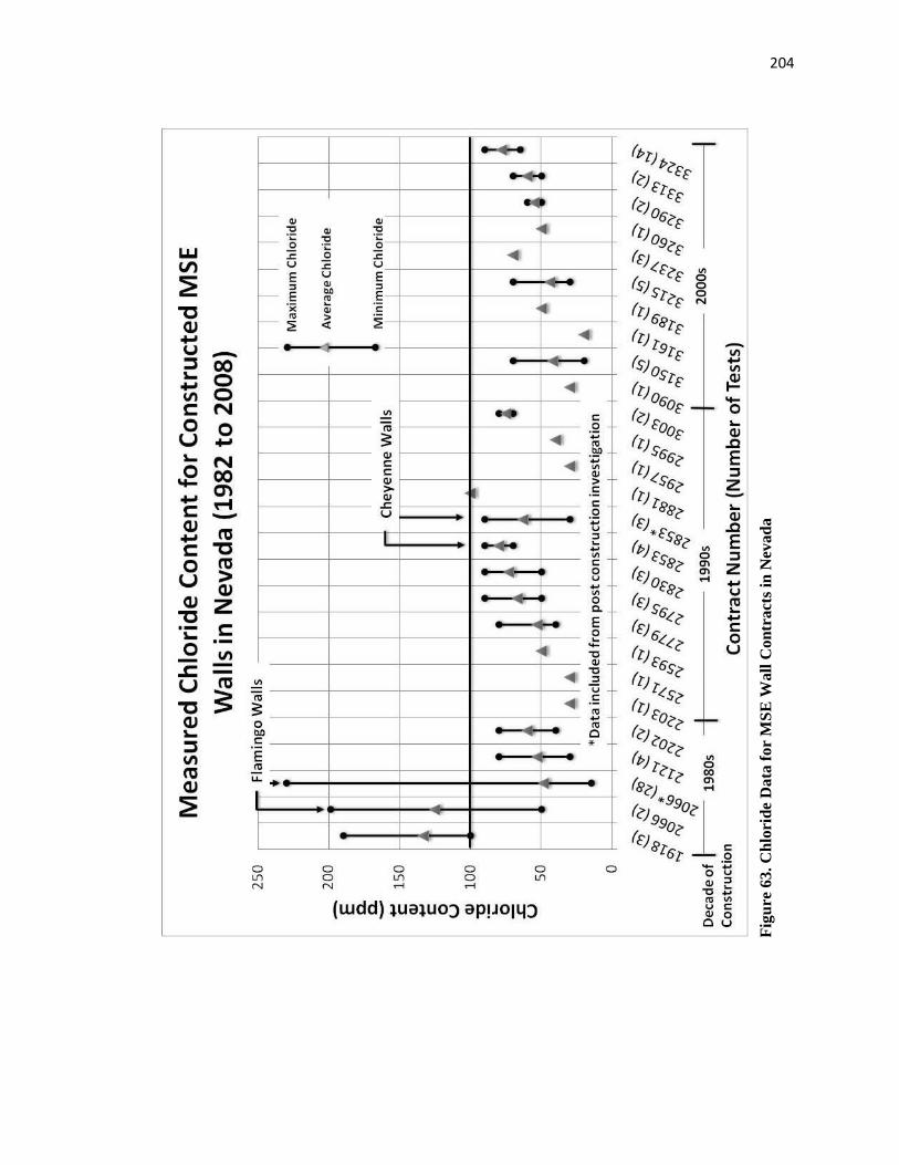
204

Fig

ure

63.

Ch

lori

de

Data

for

MS

E W

all

Con

tract

s in

Nev

ad

a

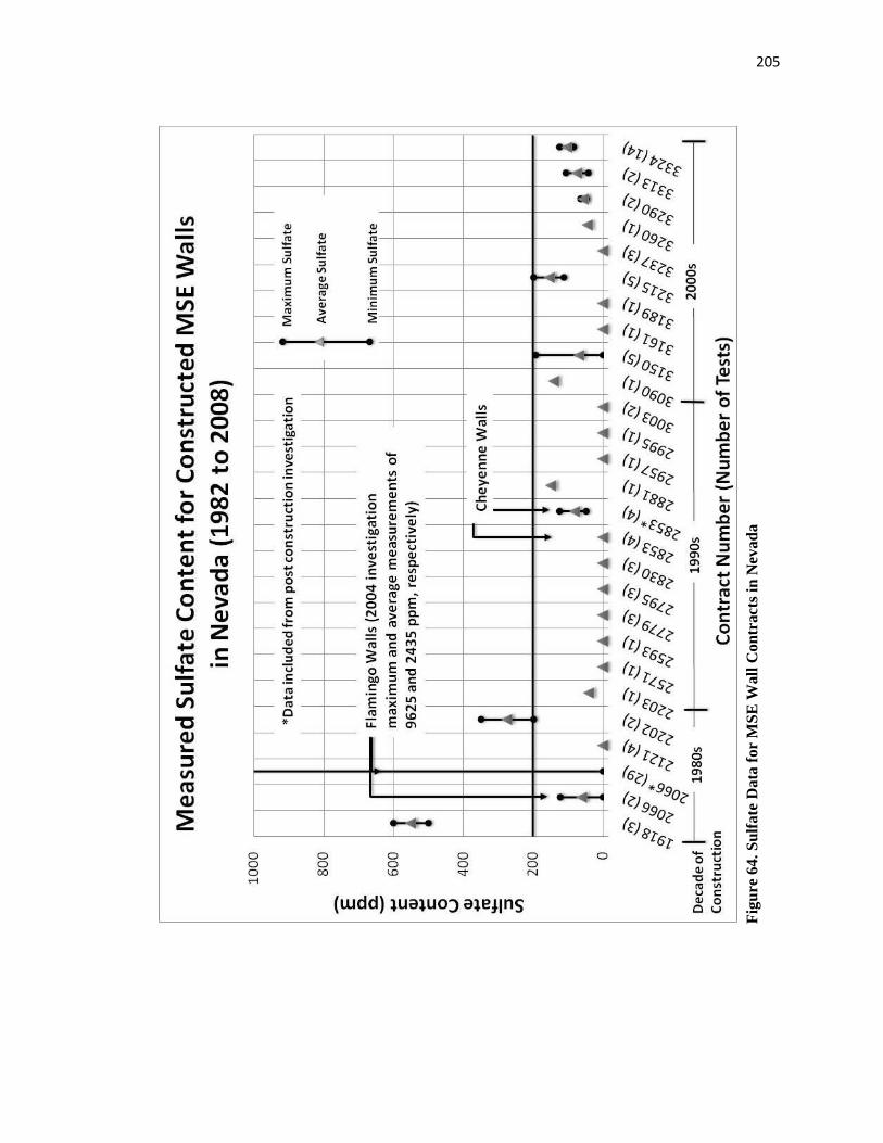
205

Fig

ure

64

. S

ulf

ate

Da

ta f

or

MS

E W

all

Con

tract

s in

Nev

ad

a

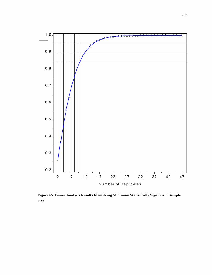
206

Figure 65. Power Analysis Results Identifying Minimum Statistically Significant Sample

Size

GROUP cv15ef20111

Po

we

r

0 .2

0.3

0.4

0.5

0.6

0.7

0.8

0.9

1.0

Num ber of Rep licates

2 7 12 17 22 27 32 37 42 47

1

1

1

1

1

1

1

1

1

1

1

11

11

1 1 1 1 1 1 1 1 1 1 1 1 1 1 1 1 1 1 1 1 1 1 1 1 1 1 1 1 1 1 1

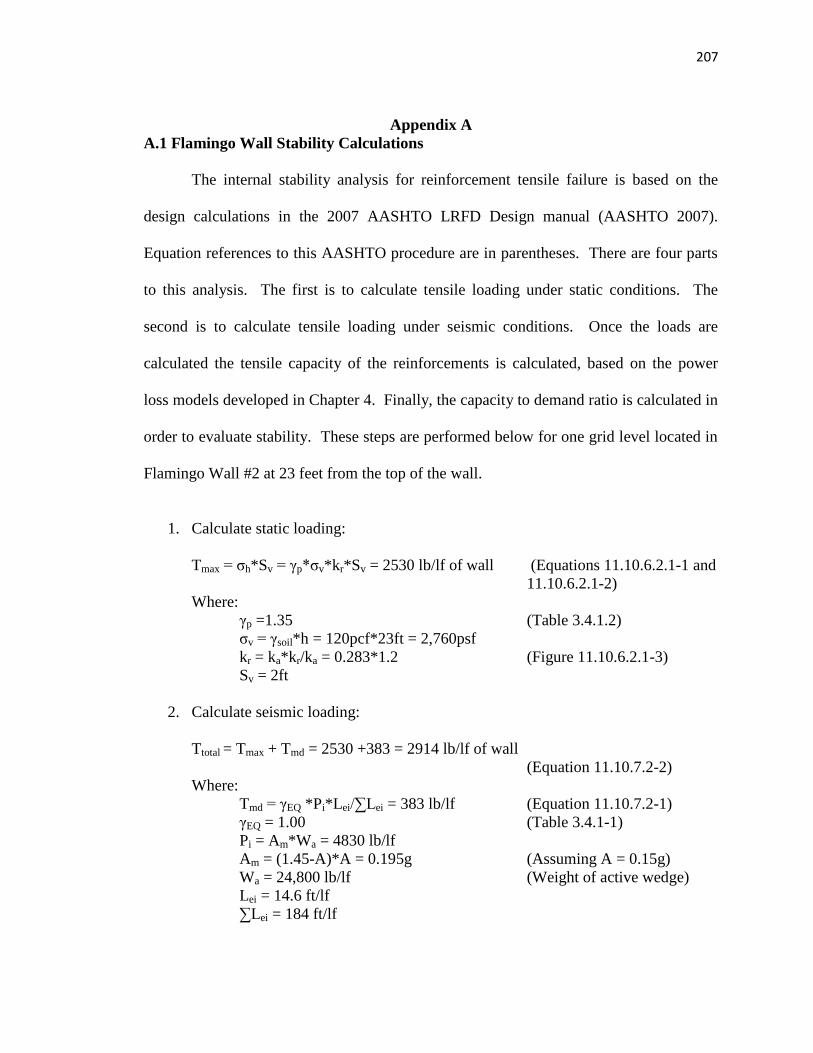
207

Appendix A

A.1 Flamingo Wall Stability Calculations

The internal stability analysis for reinforcement tensile failure is based on the

design calculations in the 2007 AASHTO LRFD Design manual (AASHTO 2007).

Equation references to this AASHTO procedure are in parentheses. There are four parts

to this analysis. The first is to calculate tensile loading under static conditions. The

second is to calculate tensile loading under seismic conditions. Once the loads are

calculated the tensile capacity of the reinforcements is calculated, based on the power

loss models developed in Chapter 4. Finally, the capacity to demand ratio is calculated in

order to evaluate stability. These steps are performed below for one grid level located in

Flamingo Wall #2 at 23 feet from the top of the wall.

1. Calculate static loading:

Tmax = σh*Sv = γp*σv*kr*Sv = 2530 lb/lf of wall (Equations 11.10.6.2.1-1 and

11.10.6.2.1-2)

Where:

γp =1.35 (Table 3.4.1.2)

σv = γsoil*h = 120pcf*23ft = 2,760psf

kr = ka*kr/ka = 0.283*1.2 (Figure 11.10.6.2.1-3)

Sv = 2ft

2. Calculate seismic loading:

Ttotal = Tmax + Tmd = 2530 +383 = 2914 lb/lf of wall

(Equation 11.10.7.2-2)

Where:

Tmd = γEQ *Pi*Lei/∑Lei = 383 lb/lf (Equation 11.10.7.2-1)

γEQ = 1.00 (Table 3.4.1-1)

Pi = Am*Wa = 4830 lb/lf

Am = (1.45-A)*A = 0.195g (Assuming A = 0.15g)

Wa = 24,800 lb/lf (Weight of active wedge)

Lei = 14.6 ft/lf

∑Lei = 184 ft/lf

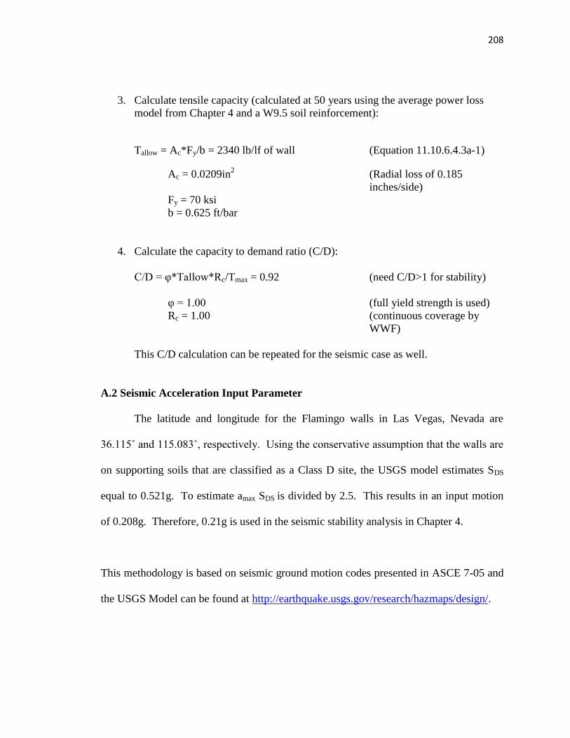
208

3. Calculate tensile capacity (calculated at 50 years using the average power loss

model from Chapter 4 and a W9.5 soil reinforcement):

Tallow = Ac*Fy/b = 2340 lb/lf of wall (Equation 11.10.6.4.3a-1)

Ac = 0.0209in2 (Radial loss of 0.185

inches/side)

Fy = 70 ksi

b = 0.625 ft/bar

4. Calculate the capacity to demand ratio (C/D):

C/D = φ*Tallow*Rc/Tmax = 0.92 (need C/D>1 for stability)

φ = 1.00 (full yield strength is used)

Rc = 1.00 (continuous coverage by

WWF)

This C/D calculation can be repeated for the seismic case as well.

A.2 Seismic Acceleration Input Parameter

The latitude and longitude for the Flamingo walls in Las Vegas, Nevada are

36.115˚ and 115.083˚, respectively. Using the conservative assumption that the walls are

on supporting soils that are classified as a Class D site, the USGS model estimates SDS

equal to 0.521g. To estimate amax SDS is divided by 2.5. This results in an input motion

of 0.208g. Therefore, 0.21g is used in the seismic stability analysis in Chapter 4.

This methodology is based on seismic ground motion codes presented in ASCE 7-05 and

the USGS Model can be found at http://earthquake.usgs.gov/research/hazmaps/design/.

http://earthquake.usgs.gov/research/hazmaps/design/

Documents

INVESTIGATION OF CORROSION OF MSE WALLS IN NEVADA