Embed Size (px)
Citation preview

LUND UNIVERSITY
PO Box 117221 00 Lund+46 46-222 00 00
Investigation of a Biofilm Reactor Model with Suspended Biomass
Masic, Alma
2013
Link to publication
Citation for published version (APA):Masic, A. (2013). Investigation of a Biofilm Reactor Model with Suspended Biomass.
Total number of authors:1
General rightsUnless other specific re-use rights are stated the following general rights apply:Copyright and moral rights for the publications made accessible in the public portal are retained by the authorsand/or other copyright owners and it is a condition of accessing publications that users recognise and abide by thelegal requirements associated with these rights. • Users may download and print one copy of any publication from the public portal for the purpose of private studyor research. • You may not further distribute the material or use it for any profit-making activity or commercial gain • You may freely distribute the URL identifying the publication in the public portal
Read more about Creative commons licenses: https://creativecommons.org/licenses/Take down policyIf you believe that this document breaches copyright please contact us providing details, and we will removeaccess to the work immediately and investigate your claim.
INVESTIGATION OF A BIOFILM REACTOR
MODEL WITH SUSPENDED BIOMASS
ALMA MASIC
Faculty of EngineeringCentre for Mathematical Sciences
Mathematics

MathematicsCentre for Mathematical SciencesLund UniversityBox 118SE-221 00 LundSweden
http://www.maths.lth.se/
Doctoral Theses in Mathematical Sciences 2013:1ISSN 1404-0034
ISBN 978-91-7473-465-2LUTFMA-1047-2013 © Alma Masic, 2013
Printed in Sweden by MediaTryck, Lund 2013
Abstract
Biofilms are compact, sessile microbial communities that attach to surfaces in aqueousenvironments. In wastewater treatment, they are especially important for removal ofphosphorus and nitrogen, which, if released into a receiving water body, can cause severeeutrophication. Mathematical models of biofilms in wastewater are used to understandthe underlying processes and to describe and analyze biofilm development. Althoughbiofilm reactors always contain an amount of suspended biomass, this biomass is mostlyneglected in mathematical models of biofilm reactors. This thesis is based on four paperswhich investigate the role of suspended biomass in biofilm reactors. A one-dimensionalmathematical model of biofilm and suspended biomass in a continuous stirred tank reac-tor is presented and analyzed in the first paper. The underlying model is a hybrid modelof chemostat-like mass balances for the substrate and biomass in the reactor, coupled witha free boundary value problem for the substrate in the biofilm. In a single species singlesubstrate setting, stability conditions for washout and persistence are given. It is foundthat biofilm and suspended biomass are either both present in the reactor or completelywashed out. Numerical simulations show that biofilm dominates over suspended biomassin the longterm reactor performance, but that suspended biomass is relatively more effi-cient at substrate removal. The model is extended to a microbially and algebraically morecomplex multi-species multi-substrate model in the third paper, describing two-step ni-trification in a Moving Bed Biofilm Reactor (MBBR). Nitrogen enters the reactor in theform of ammonium and leaves as nitrate after an intermediate conversion to nitrite. Nu-merical simulations show that suspended biomass does not contribute significantly to theoverall reactor performance, but is substantial in the intermediate processes. In the secondpaper, the biofilm model is numerically validated against microelectrode measurements ofoxygen gradients across the biofilm depth of a nitrifying biofilm attached to a suspendedcarrier harvested from an MBBR. Finally, a single species single substrate case with a lim-ited amount of substrate and treatment time is considered as a two-objective optimizationproblem. With the bulk flow velocity as the control, different classes of admissible func-tions are investigated. It is found that, given the uncertainties in the initial data, noneof the other functions perform better than the constant flow rate, i.e. the uncontrolledreactor.
iii

iv
Populärvetenskapligsammanfattning
Hantering av avlopp och avfall är en del av alla människors vardag. Vår hälsa och miljöpåverkas av metoderna vi tillämpar för att ta hand om rester från hushåll och industrier.Genom teknikens utveckling används idag bakterier i vattenreningsverk där avloppsvat-ten renas från alla skadliga föremål och föreningar. Med hjälp av matematiska uttryck ochanalyser, i samspel med biologiska, fysikaliska och kemiska experiment, kan dessa ren-ingsprocesser undersökas och förhoppningsvis förbättras. I den här avhandlingen vändsstrålkastarljuset mot så kallade biofilmer, som är betydande för borttagning av kväve ochfosfor ur avloppsvatten.
Bakterier som hopar sig på en blöt yta bildar ofta biofilmer med helt andra egenskaperän de fria bakterierna. Biofilmer skyddar bakterierna från exempelvis antibiotika, men debromsar samtidigt tillflödet av näringsämnen. Ett typexempel på biofilmer är vanligtplack som bildas på tänderna. Om placken inte tas bort kan den bilda tandsten ochorsaka karies. Trots att biofilmer ofta kopplas samman med sjukdomar och förfall finnsdet flera användningsområden där de kan göra nytta.
I avloppsvattenrening har man länge använt bakterier i form av aktivt slam, där bak-terierna växer och förökar sig genom att bryta ner olika näringsämnen som finns i avlopps-vattnet. En pågående övergödning av vattendrag på grund av för höga halter av kväve ochfosfor i reningsverkens utloppsvatten ökar kraven på förbättrade reningsmetoder. Ett sättatt ytterligare rena avloppsvattnet är att använda biofilmer som ger utrymme för specialis-erade bakterier att bryta ner kväve och ta upp fosfor. Kväve kommer in till reningsverketi form av ammonium som finns i urin och lämnar det slutligen som oskadlig kvävgas.
Matematiska modeller i form av differentialekvationer har länge använts för att beskrivaoch förstå bakteriernas mekanismer och deras roll i reningen av vatten. Modellerna vari-erar i komplexitet och detaljrikedom beroende på hur många element och processer debeskriver. Många är därför mycket komplicerade och svåra att lösa analytiskt och måsteberäknas numeriskt med hjälp av datorer. Enklare modeller, där många mindre viktigaprocesser försummas, kan däremot ofta studeras med exakt matematik.
v
Biofilmssystem i vattenreningsverk brukar alltid ha en liten andel bakterier som flyteromkring i vattnet. Dessa bakterier, så kallad suspenderad biomassa, kommer antingenin till reaktorn med det orenade vattnet eller lossnar från biofilmen. Den suspenderadebiomassan måste tas bort från det renade vattnet innan det kan fortsätta vidare i ren-ingsverket och ut till ett vattendrag. Trots detta försummas den fria biomassan oftast itraditionella biofilmsmodeller.
I den här avhandlingen undersöks effekterna av suspenderad biomassa i matematiskabiofilmsmodeller av avloppsvattenrening. En relativt enkel endimensionell modell meden bakteriesort och ett näringsämne presenteras och analyseras både analytiskt och nu-meriskt. Det visar sig att suspenderad biomassa och biofilm måste samexistera. I ettlängre tidsperspektiv kommer biofilmen att dominera den suspenderade biomassan. Sus-penderad biomassa är dock relativt sett bättre på att bryta ner näringsämnet än biofilmmen effekten är oftast obetydlig eftersom dess andel i allmänhet är ganska liten.
En mer varierande bild ges av en nitrifikationsmodell där två olika bakteriesorter ochtre näringsämnen samt syre finns i reaktorn. Lämpliga parametrar framtogs i en förstastudie där simulerade syrekoncentrationer jämfördes med uppmätta tvärs igenom biofil-men. Ytterligare numeriska simuleringar visar att reaktorns totala prestanda inte påverkasnämnvärt av suspenderad biomassa i och med att biofilmen står för störst andel nedbryt-ning. Däremot spelar den suspenderade biomassan en tydlig roll i processens mellanstegoch mellanprodukter. Slutsatsen är att suspenderad biomassa inte behöver inkluderas ibiofilmsmodeller om reaktorns prestationsförmåga står i fokus.
I en efterföljande studie undersöks vad som händer i en situation där tillgången tillnäringsämnet samt behandlingstiden är begränsade. Frågan ställs om en sådan reaktor kanförbättras genom styrning av flödet mellan förvaringsreaktorn och behandlingsreaktorn.Ett optimerat styrningsproblem formuleras och löses för olika typer av flödesreglering.Den bästa kandidaten, en så kallad off-on-funktion där flödet är avstängt till en börjanmedan bakterierna etablerar sig, är inte avsevärt bättre än ett vanligt konstant flöde. Slut-satsen blir att ett styrt flöde inte har några nämnvärda fördelar gentemot en konstantflödeshastighet.
vi

Preface
This thesis considers the problem of mathematical modeling of biofilm reactors whichinclude suspended biomass. Such a model is formulated and analyzed both mathemati-cally and numerically in the first paper. The next paper investigates a nitrifying biofilmin a Moving Bed Biofilm Reactor through microelectrode measurements and numericalsimulations. In the third paper the main model from the first paper is used and extendedby introduction of microbial and physical complexity from the nitrification model of thesecond paper. The extended model is analyzed by means of extensive numerical simula-tions. In the last paper an optimization problem is presented and studied. The aim of theproblem is to find a flow regime between a storage reactor and a treatment reactor thatwill increase the substrate removal efficiency and decrease process duration.
The work of this thesis has been funded by the Knowledge Foundation, Malmö Uni-versity and Lund University.
The thesis consists of the following four papers:
I A. Mašic and H.J. Eberl, (2012), "Persistence in a single species CSTR modelwith suspended flocs and wall attached biofilms", Bulletin of Mathematical Biology,74(4):1001-1026.
II A. Mašic, J. Bengtsson and M. Christensson, (2010), "Measuring and modelingthe oxygen profile in a nitrifying Moving Bed Biofilm Reactor", Mathematical Bio-sciences, 227(1):1-11.
III A. Mašic and H.J. Eberl, (Aug 2012), "A modeling and simulation study of the roleof suspended microbial populations in nitrification in a biofilm reactor", submittedto Bulletin of Mathematical Biology.
IV A. Mašic and H.J. Eberl, (Feb 2013), "On optimization of substrate removal in abioreactor with wall attached and suspended bacteria", submitted to MathematicalBiosciences and Engineering.
vii

viii
Acknowledgments
I have had the privilege to meet and interact with various people during my years as aPhD student, many of whom have contributed to make this journey worthwhile. First,I would like to thank my supervisors Per Ståhle and Johan Helsing for all their helpand advice. Their constructive comments during the examination of this thesis haveconsiderably improved its quality. I would also like to acknowledge the help from myprevious supervisors Anders Heyden and Niels Christian Overgaard.
I will forever be most indebted to Hermann Eberl of University of Guelph, Canada.He has been my main collaborator, providing genuine support and guidance along theway. His enthusiasm for and knowledge of mathematics have been contained in countlesse-mails and long discussions, which have been crucial for my work. I would particularlylike to emphasize the amount of work he has invested in the finalization of this thesis, withan unfailing attention to detail. Collaboration with such a generous and inspiring personcontinues to be effortless and I hope we will have plenty of opportunities to work togetheragain. I would also like to thank him for inviting me to visit Guelph and devoting his timeto our discussions during my research stays. My visits were greatly eased by the assistanceand kindness of Mallory Frederick Jutzi, Hedia Fgaier, Ranga Sudarsan, Vardayani Ratti,Blessing Uzor, Fazal Abbas and Sandy Smith, who all welcomed me as one of their own.
My interdisciplinary work would have been a mystery were it not for the considerablehelp and support I have received from Magnus Christensson, Jessica Bengtsson, MariaJohansson, Eva Tykesson and Jenny Kruuse at AnoxKaldnes in Lund. They have pa-tiently taught me so much about biofilms and wastewater treatment, always providingexplanations for a curious mathematician. I would also like to express my gratitude totheir colleagues who have shown a friendly work environment and invited me to eat many"fredagsbulle" over the years.
I am sincerely thankful for the generosity and understanding shown by Kalle Åströmat the Centre for Mathematical Sciences. Andrey Ghulchak contributed with ideas andhelpful conversations, which I truly appreciate. Furthermore, I want to thank MikaelAbrahamsson at the mathematical library, who has eagerly helped me find many impor-tant, but obscure books and papers. I have had several interesting discussions with RobertAlmstrand, Malte Hermansson and Fred Sörensson of Gothenburg University and would
ix
like to thank them for all their competent and insightful comments.I was fortunate to be able to share my experience with fellow graduate students Mat-
tias Hansson and Ketut Fundana. They have selflessly provided support and encourage-ment, especially during the rough patches of this project. The help of Sami Brandt, whostarted out as a post-doc and became a friend of ours, is highly appreciated. I will miss allour joint activities, many of which have turned into anecdotes. Good future to all of us!
Christina Bjerkén and Ulf Hejman of Malmö University showed enthusiasm andcompetence during our short collaboration, which I am very grateful for. It has also beena pleasure to spend time with the graduate students involved in the research programBiofilms – Research Center for Biointerfaces at Malmö University.
Without my family and friends, who have provided endless support and appreciation,I would not have been where I am today. I will always cherish the love and kindness theyhave shown me.
Stort tack till mina kära vänner Arsine Bellarian, Džana Džemidžic, Karin Fremlingoch Aida Hadžialic som alltid har trott på mig. Den här avhandlingen hade inte blivit såbra utan det villkorslösa stöd ni har givit mig. Även Šeherzada Catak och Berina Ibrovichar hjälpt mig och stöttat mig. Jag är lyckligt lottad som har sådana underbara vänner.
Ich bedanke mich auch herzlich bei Maren Kus, für ihre Freundschaft, Unterstützung,Aufmerksamkeit und Gastfreundschaft.
Mojim dragim roditeljima Fatimi i Ramizu, najvece hvala na podršci i povjerenju kojesu mi pokazali. Vaša beskonacna ljubav, pomoc i bodrenje su mi olakšali i omogucili putkroz moje dugogodišnje školovanje. Pružili ste mi veliki oslonac u životu i uvijek ste setrudili da osigurate bolju buducnost za mene i za Adnana. Zbog toga cu vam vjecnobiti zahvalna i ponosna na sve što sam postigla. Moj lijepi i voljeni brat Adnan mi jetakoder uvijek pružao podršku i pomoc, na cemu sada iskreno zahvaljujem (yoshi hugs!).Nana Ružica i deda Ismet su s ponosom i ljubavlju pratili moje uspjehe, ohrabrivali mei podupirali. Deda bi sada sigurno bio presretan da je docekao objavljivanje mog rada.Hvala vam oboma na potpori. Takoder zahvaljujem mojoj dragoj tetki Melihi, tetkuSamiru i rodicama Nejli, Sabini i Emini, koji su bili uz mene, pružali mi pomoc i pov-jerenje. Hvala i ostaloj rodbini u Bosni i Hercegovini i širom svijeta.
Posebno hvala mojim prijateljima na velikodušnoj podršci: Ajana Sadikovic, AjdinSadikovic, Irma Hodžic i Zlatan Balta, Lamija i Edin Karabegovic, Mehmed Jakic, MirzaJelacic, Senad Zjajo.
Podršku mi je takoder pružila i porodica Colo. Konacno hvala mom dragom Atifu,koji je bio uz mene u dobru i u zlu, uvijek sa velikim razumijevanjem i dubokom ljubavlju.Tvoja podrška, pamet, nježnost i briga su mi mnogo znacile. Ti si jedna poduzetna imaštovita duša, koja me inspiriše i motiviše. Hocemo li sada na more?
x

Contents
Abstract iii
Populärvetenskaplig sammanfattning v
Preface vii
Acknowledgments ix
1 Introduction 11.1 Background . . . . . . . . . . . . . . . . . . . . . . . . . . . . . . . 11.2 Overview of the thesis . . . . . . . . . . . . . . . . . . . . . . . . . . 2
2 Biofilms in wastewater treatment 72.1 Biofilms . . . . . . . . . . . . . . . . . . . . . . . . . . . . . . . . . 7
2.1.1 Heterogeneity: spatial structure, diffusion gradients and micro-bial populations . . . . . . . . . . . . . . . . . . . . . . . . . 9
2.1.2 Harmful and beneficial biofilms . . . . . . . . . . . . . . . . . 142.1.3 Attachment and detachment . . . . . . . . . . . . . . . . . . 15
2.2 Wastewater treatment . . . . . . . . . . . . . . . . . . . . . . . . . . 172.2.1 Moving Bed Biofilm Reactor . . . . . . . . . . . . . . . . . . 192.2.2 Nitrification . . . . . . . . . . . . . . . . . . . . . . . . . . . 20
3 Biofilm modeling 233.1 Mathematical models in biology . . . . . . . . . . . . . . . . . . . . . 23
3.1.1 Chemostat . . . . . . . . . . . . . . . . . . . . . . . . . . . . 243.1.2 Conservation of mass, diffusion and transport . . . . . . . . . . 27
3.2 Biofilm models . . . . . . . . . . . . . . . . . . . . . . . . . . . . . . 293.2.1 Overview . . . . . . . . . . . . . . . . . . . . . . . . . . . . 293.2.2 The one-dimensional Wanner-Gujer model . . . . . . . . . . . 303.2.3 Biofilm models in wastewater applications . . . . . . . . . . . . 32
xi

3.2.4 Advantages and disadvantages of simple models . . . . . . . . . 36
4 Conclusions and outlook 43
Bibliography 47
Paper I 59
Paper II 90
xii
Chapter 1
Introduction
1.1 Background
Biofilms are ubiquitous microbial aggregates that coat surfaces in an aqueous environ-ment. As aggregates they exhibit different features than free floating cells, for examplean increased antibiotic resistance and the experience of concentration gradients from thebulk liquid toward the inner parts of the biofilm. The best and most studied example ofbeneficial biofilms is their use in wastewater treatment. Bacteria have been used in biolog-ical treatment even before biofilms were considered, for example in trickling filters, wherewastewater was trickled over a bed of rocks on which bacteria had accumulated. Thebacteria typically consume substrates from the wastewater and produce compounds thatare safe for release into the environment. Here, the term substrate is used in a biochem-ical sense, denoting a substance that provides energy for the metabolism of the bacteria.Biofilms are used in wastewater treatment to allow for slow growing bacteria to grow andremain in the reactor while treating the wastewater. Removal of nitrogen and phosphorushas increased in significance due to possible eutrophication in water bodies that receivewastewater discharges when high levels of these chemical compounds are released. Nitro-gen is, therefore, removed in an aerobic process called nitrification in which ammoniumis converted first to nitrite and then to nitrate by two different bacterial species.
Mathematical models of wastewater treatment processes and biofilms in particularhave been used to understand the underlying mechanisms and structures of these com-plex processes. The more we learn about biofilms from laboratory studies the more com-ponents we can incorporate into our models. On the other hand, the results from amathematical study (either analytical or numerical) may confirm hypotheses or ask newquestions which close the loop in a symbiotic relationship between experimentalists andmathematicians. There now exist all kinds of different models ranging from simple one-dimensional to complicated three-dimensional descriptions of biofilm wastewater pro-
1
CHAPTER 1. Introduction
cesses. Simpler models allow for more analysis, but may often lack in proper descriptionof biofilm structure or heterogeneity. Complicated models involve many components andproduce a detailed multi-dimensional description and can often only be solved numeri-cally using large computation power.
Biofilm systems always have a certain amount of suspended biomass present in thereactor, even if it is much less than the biomass found in an activated sludge reactor.The suspended biomass, a result of detachment from the biofilm and possibly addition ofbiomass through the influent, can (re-)attach to the biofilm. However, traditional biofilmmodels have typically neglected the existence and effects of suspended biomass in thereactor, even when the detachment process is included. While this can be a reasonableassumption for certain lab-scale reactors in which suspended biomass is almost immedi-ately washed out, it may be important for biofilm reactors where the suspended biomassis retained long enough for (re-)attachment to occur, which influences biofilm growth.
The main objective of this thesis is to investigate the role of suspended biomass inbiofilm reactor models. Suspended biomass and biofilms interact through attachmentand detachment of bacterial cells. In this thesis, the following questions, among others,are asked: How much does suspended biomass contribute to the reactor performance?Which mode of growth will dominate, sessile or suspended? Is it possible for the twobiomass forms to out-compete each other? When is it necessary to include suspendedbiomass in biofilm models?
The investigation is based on a dynamic one-dimensional mathematical model ofbiofilm and suspended biomass in a continuous stirred tank reactor, which is presentedin this thesis. The model is mathematically and numerically analyzed. Furthermore,the single species single substrate model is extended through incorporation of microbialcomplexity in order to represent a nitrifying moving bed biofilm reactor in a wastewa-ter setting. The nitrification model is assessed through comparison with microelectrodemeasurements of oxygen concentration gradients. Finally, optimization of a bioreactor bycontrol of the flow rate is investigated.
1.2 Overview of the thesis
Due to the interdisciplinarity of the thesis, the biological background is given in Chapter2 and the mathematical framework in Chapter 3. Both chapters are mainly intendedas an overview of the research field and to provide the necessary context for the prob-lems addressed in the papers. Conclusions and future work are presented in Chapter 4.The scientific contributions of this thesis are contained in the four papers that follow inthe last part of the thesis. They are also summarized here below with specified authorcontributions.
2

1.2. Overview of the thesis
PAPER I — Persistence in a single species CSTR model with suspendedflocs and wall attached biofilms
Alma Mašic and Hermann Eberl
In this paper we investigate the role of suspended biomass in a biofilm reactor. Weformulate and study a one-dimensional mathematical model of suspended and wall-attached microbial populations and resource dynamics in a continuous stirred tank reac-tor (CSTR). The starting model is a free boundary value problem for a parabolic partialdifferential equation which we formally can rewrite as a model of ordinary differentialequations (ODE) and then study with elementary ODE techniques. For a single speciessingle substrate setting our analysis shows that the stability of the washout equilibriumdepends on the dilution rate and on the growth and decay rates of the suspended flocsand the biofilm. We compare our results with the algebraically and physically less com-plex Freter model (a model of a chemostat with wall-attachment) and find that the Freterresults largely carry over. If the trivial equilibrium is unstable the system will attain a non-trivial equilibrium at which biomass is present in the reactor in both modes of growth.Numerical simulations show that biofilms will dominate as mode of growth in a majorityof the studied cases. The longterm behavior of the system depends on operating condi-tions of the reactor. Furthermore, it is observed that suspended biomass is relatively moreefficient at substrate removal than biofilms are.
Author contribution: AM and HE constructed the model, developed the theoryand analyzed the results. AM implemented the model and outlined and performed thenumerical experiments. Manuscript was written and reviewed by AM and HE.
PAPER II — Measuring and modeling the oxygen profile in a nitrify-ing Moving Bed Biofilm Reactor
Alma Mašic, Jessica Bengtsson and Magnus Christensson
In this paper we validate the nitrification model against experimental data and identify re-alistic parameters for the model. We demonstrate an experimental microelectrode setup,used to measure oxygen gradients in a nitrifying biofilm on a suspended carrier from aMoving Bed Biofilm Reactor (MBBR) at different flow velocities. We incorporate theCSTR equation into a mathematical biofilm model of Wanner-Gujer type and simulatethe oxygen gradients numerically with model parameters from several sources. The un-derlying biofilm model is a combined hybrid-parabolic free boundary value problem forwhich validation of parameters suggested in the literature and identification of parametersthat are unique to this setup are performed. Our results show a dependence of biofilmand mass transfer boundary layer thickness on the bulk flow rate, implying that a decreaseof the boundary layer would enhance the utilization of oxygen. Moreover, we establish arelationship between the erosion parameter and the bulk flow rate.
3

CHAPTER 1. Introduction
Author contribution: JB designed and performed the microelectrode measurements,AM constructed the model and developed and performed the numerical simulations. AMand JB analyzed and interpreted the results and wrote and reviewed the manuscript withcontributions from MC.
PAPER III — A modeling and simulation study of the role of sus-pended microbial populations in nitrification in a biofilm reactor
Alma Mašic and Hermann Eberl
The presence and effects of suspended biomass in biofilm reactors are usually neglected intraditional biofilm models. We therefore investigate the importance of suspended biomassin a nitrifying biofilm reactor. In this paper we introduce the microbial complexity fromPaper II into the model presented in Paper I, i.e. we study a one-dimensional mathemat-ical model of a nitrifying MBBR with biofilms and suspended biomass. The resultingmodel is an ODE system that is coupled to a hyperbolic free boundary value problem bya semi-linear system of second order two-point boundary value problems. The complex-ity of the model prevents extensive analysis thereof but allows for numerical simulations.Our results show that the incorporation of suspended biomass may be neglected if the ob-jective of the study is the overall reactor performance. However, inclusion of suspendedbiomass would be significant if detailed descriptions of the intermediate steps and prod-ucts of the nitrification process are required.
Author contribution: AM constructed the model and analyzed the results with ad-vice from HE. AM implemented the model and outlined and performed the numericalexperiments. Manuscript was written and reviewed by AM and HE.
PAPER IV — On optimization of substrate removal in a bioreactorwith wall attached and suspended bacteria
Alma Mašic and Hermann Eberl
In Papers I and III we assumed an infinite supply of substrate and studied longterm effectswith regard to suspended biomass in a biofilm reactor. In this paper we pose an optimiza-tion problem for the one-dimensional single species single substrate model presented inPaper I with the aim to increase substrate removal efficiency and decrease process dura-tion. We assume that a storage tank with a limited amount of substrate is connected to thebiological treatment reactor through a controllable flow. The resulting optimal controlproblem is singular and leads to chattering control, which is not feasible from a practi-cal perspective. Our results show that the optimization problem is rather insensitive tochanges in the flow rate that deviate from the constant flow rate. We compute numericalsolutions for specific off-on flow rate functions and find that they marginally improve the
4

1.2. Overview of the thesis
reactor performance. Since they depend on initial data which cannot be controlled, wepropose that a search for a different control than the constant flow rate is not necessary.
Author contribution: AM and HE constructed the model, developed the theoryand analyzed the results. AM implemented the model and outlined and performed thenumerical experiments. Manuscript was written and reviewed by AM and HE.
5

CHAPTER 1. Introduction
6

Chapter 2
Biofilms in wastewater treatment
2.1 Biofilms
Bacteria are prokaryotic microorganisms that are found in abundance almost everywhereon Earth. Many of them play a crucial role in nutrient cycles and human health, whileothers are detrimental to the environment and our well-being. With increased knowl-edge about the ubiquity and diversity of biofilms, improved investigative methods andinterdisciplinary approaches, the biofilm research field has grown significantly since thebeginning of the 1980s. Biofilms are most easily defined as layered aggregates of micro-bial populations attached to each other or to solid surfaces in aqueous environments orsubmerged in a liquid [16, 18]. They are typically embedded in a gel-like matrix (EPS,extracellular polymeric substances) produced by the bacteria themselves, comprised ofpolysaccharides, proteins, extracellular DNA etc. [33]. Together they form a very com-plex and differentiated community with a behavior unlike that of planktonic bacteria[119]. Although this description may appear very broad, it captures something that iscommon to all biofilms. Apart from that, what identifies biofilms is their wide diver-sity and adaptation to many different situations. For example, biofilms occur naturallyin human bodies (e.g. as dental plaque), in household plumbing, on ship hulls, in hotsprings, on frozen glaciers along with other locations [17]. Biofilms are in some way moredifferent than they are similar.
A typical biofilm development has three stages: (i) attachment, (ii) growth, (iii) de-tachment, see Figure 2.1. In the initial attachment phase, bacteria adhere to coated solidsurfaces, among which we find both organic and inorganic materials [9, 106]. The wetsurfaces are coated with a thin film consisting of nutrients, proteins and other molecules,to which microbial cells adsorb. They initiate production of EPS, which entraps nutrients,microbial products and other organic and inorganic matter. This leads to an irreversiblemode of attachment and a commencing aggregation.
7

CHAPTER 2. Biofilms in wastewater treatment
Figure 2.1: The three stages of biofilm development. Image used with permission, cour-tesy of Peg Dirckx, Montana State University.
During the second stage of biofilm growth and maturation, the bacteria within thebiofilm experience an environment much different from that of planktonic bacteria. TheEPS matrix surrounds and protects the biofilm bacteria, provides nutrients and "neigh-bors" who can communicate through cell-to-cell signaling (quorum sensing) [81]. Thebiofilm attains a complex three-dimensional dynamic structure. It is throughout this stagethat biofilms develop their heterogeneous traits, such as structural diversity and distribu-tion of populations.
The final stage of the biofilm development contains detachment of cells into thesurrounding medium. Detachment processes can roughly be divided into an active and apassive form [50]. The latter involves external forces such as shear stresses, predation byhigher organisms etc. which cause a loss of biomass. Cells can leave the biofilm structureindividually or in larger clumps. Active detachment is initiated by the bacteria internally,leading to a dispersal of cells. Detached cells are able to attach and form new coloniesdownstream of the biofilm that they originated from.
What distinguishes biofilms from free floating bacteria are mainly three features,namely: the gel-like EPS-matrix that encapsulates the microorganisms within a biofilmand provides a specific environment, the exposure to concentration gradients of dissolvedcomponents across a biofilm instead of bulk liquid concentrations, and the very difficulteradication of biofilms that exhibit a strong resistance to antibiotics and drugs [20]. Thus,biofilms are able to survive in many different environments where free floating bacteriawould be eliminated, wherefore bacteria preferentially reside in biofilms.
The following sections will only cover those elements of biofilm literature that providea context and are relevant to this dissertation, rather than presenting an extensive literatureoverview.
8

2.1. Biofilms
Figure 2.2: Typical biofilm mushroom-like structure with liquid channels. Image usedwith permission, courtesy of Peg Dirckx, Montana State University.
2.1.1 Heterogeneity: spatial structure, diffusion gradients and mi-crobial populations
A mature biofilm is very responsive to its surroundings and is able to adapt to externalchanges. As a result, biofilms express various features in chemical, biological and physio-logical composition as well as structural arrangement [105], which have been observablethrough advances in microbiological and in particular microscopic tools. The confocallaser scanning microscope (CLSM) has notably enabled studies and visualizations of liv-ing, functional and hydrated biofilms more or less in their natural form.
Spatial structure
In the initial phases of biofilm formation the bacteria constitute a thin and patchy layer,which does not yet provide all the benefits of a joint sessile mode of growth, like protectionof washout. The length scale of a bacterium is in the range of micrometers, wherefore theearly biofilm is only a couple of micrometers thick. However, as the biofilm matures, itreaches thicknesses in the range of millimeters and on some occasions even centimeters.To the naked eye a biofilm is often perceived as a slime layer. Bacteria within a biofilm areencapsulated by the EPS matrix which is interspersed with water channels that providetransport of nutrients and other molecules throughout the complex structure [23].
The three-dimensional structure of a biofilm generally depends on the environmentin which the biofilm is situated [121]. Substrate concentration and availability (or dosageintervals in laboratory experiments) along with hydrodynamic conditions are among the
9

CHAPTER 2. Biofilms in wastewater treatment
factors that affect biofilm formation and development. A typical image of a biofilm is theso called mushroom structure, where liquid channels penetrate the bottom of the porousmushroom shaped biomass [110], see Figure 2.2. In Figure 2.3 a variety of differentbiofilm structures is shown, ranging from thin and dense to thick and porous biofilmswhich are attached to plastic surfaces in a wastewater treatment environment. The colorof the biofilm varies depending on the type of bacteria, on chemical reactions that takeplace in the biofilm and on the properties of the surrounding liquid.
Figure 2.3: Photographs of various biofilms attached to white plastic surfaces in wastew-ater treatment. The plastic walls are approximately 0.1 to 0.15mm thick and 0.2 to0.5mm long. Images used with permission, courtesy of AnoxKaldnes, Sweden.
Diffusion gradients
In diffusion, particles move from areas with high concentration to areas with low concen-tration down the concentration gradient without fluid motion. This process requires noinput of energy from the particles and is, therefore, often called a passive process which ismuch slower than advection (transport of solutes within a fluid by its bulk flow). A porousbiofilm with water channels as depicted in Figure 2.2 allows advection even within the ag-gregate. On the other hand, in a cell cluster where bacteria are densely packed advectioncannot take place due to physical obstacles, wherefore substrates must be transported intoand through the aggregate by diffusion. As a consequence, diffusion limitation arises inbiofilm systems as the diffusion distance increases substantially across a complex biofilmstructure [104].
The application of microsensor measurements in biofilm research has enabled visual-ization and direct observation of the distribution of a substrate in a living biofilm [18].
10
2.1. Biofilms
In combination with CLSM images, the heterogeneous structure of a biofilm has beenrevealed. The earliest and most studied microsensor used in biofilms was a sensor thatmeasures the oxygen concentration inside biofilms. Therefore, mostly aerobic and rela-tively thin biofilms could initially be analyzed. However, by now there exists a variety ofreliable microsensors measuring chemical composition across biofilms, e.g. pH, ammo-nium, carbon dioxide [22].
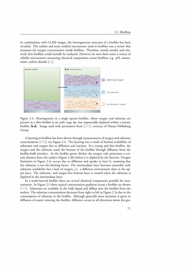
Figure 2.4: Heterogeneity in a single species biofilm, where oxygen and substrate arepresent in a thin biofilm at an early stage (a), but sequentially depleted within a maturebiofilm (b-d). Image used with permission from [105], courtesy of Nature PublishingGroup.
A layering in biofilms has been shown through measurements of oxygen and substrateconcentrations [105], see Figure 2.4. The layering was a result of limited availability ofsubstrates and oxygen due to diffusion and reaction. In a young and thin biofilm, theoxygen and the substrate reach the bottom of the biofilm through diffusion from thebiofilm-bulk interface. As the biofilm grows thicker the oxygen only penetrates a cer-tain distance from the surface (Figure 2.4b) before it is depleted by the bacteria. Oxygenlimitation in Figure 2.4c occurs due to diffusion and uptake in layer b, assuming thatthe substrate is not the limiting factor. The intermediate layer becomes anaerobic withsubstrate availability but a lack of oxygen, i.e. a different environment than in the up-per layer. The substrate- and oxygen-free bottom layer is created when the substrate isdepleted in the intermediate layer.
In a multi-layered biofilm there are several chemical components possible for mea-surement. In Figure 2.5 three typical concentration gradients across a biofilm are shown[105]. Substrates are available in the bulk liquid and diffuse into the biofilm from thesurface. The substrate concentration decreases from right to left in Figure 2.5a due to theconsumption of substrate in the biofilm. Although generally most attention is given todiffusion of matter entering the biofilm, diffusion occurs in all directions down the gra-
11
CHAPTER 2. Biofilms in wastewater treatment
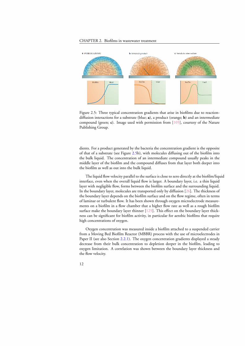
Figure 2.5: Three typical concentration gradients that arise in biofilms due to reaction-diffusion interactions for a substrate (blue; a), a product (orange; b) and an intermediatecompound (green; c). Image used with permission from [105], courtesy of the NaturePublishing Group.
dients. For a product generated by the bacteria the concentration gradient is the oppositeof that of a substrate (see Figure 2.5b), with molecules diffusing out of the biofilm intothe bulk liquid. The concentration of an intermediate compound usually peaks in themiddle layer of the biofilm and the compound diffuses from that layer both deeper intothe biofilm as well as out into the bulk liquid.
The liquid flow velocity parallel to the surface is close to zero directly at the biofilm/liquidinterface, even when the overall liquid flow is larger. A boundary layer, i.e. a thin liquidlayer with negligible flow, forms between the biofilm surface and the surrounding liquid.In the boundary layer, molecules are transported only by diffusion [26]. The thickness ofthe boundary layer depends on the biofilm surface and on the flow regime, often in termsof laminar or turbulent flow. It has been shown through oxygen microelectrode measure-ments on a biofilm in a flow chamber that a higher flow rate as well as a rough biofilmsurface make the boundary layer thinner [125]. This effect on the boundary layer thick-ness can be significant for biofilm activity, in particular for aerobic biofilms that requirehigh concentrations of oxygen.
Oxygen concentration was measured inside a biofilm attached to a suspended carrierfrom a Moving Bed Biofilm Reactor (MBBR) process with the use of microelectrodes inPaper II (see also Section 2.2.1). The oxygen concentration gradients displayed a steadydecrease from their bulk concentration to depletion deeper in the biofilm, leading tooxygen limitation. A correlation was shown between the boundary layer thickness andthe flow velocity.
12
2.1. Biofilms
Populations
Early studies of bacterial populations were based on isolation and cultivation of singlespecies bacteria on nutrient-rich media. However, many bacterial cells harvested fromnatural biofilms could not be cultured and, therefore, not studied. The turning pointto resolve this issue arrived with the employment of molecular tools, most notably insitu hybridization with rRNA probes [2]. Further combinations of fluorescence in situhybridization (FISH) with CLSM allowed identification and three-dimensional visualiza-tion and localization of microbial populations within biofilms.
Organisms, and thereby bacteria, are usually divided into groups based on the mannerthey obtain energy, their ability to fix carbon and the type of molecule they use as anelectron donor [38, Ch.1]. Organic molecules (e.g. sugars and fats) serve as electrondonors for organotrophs and inorganic molecules (e.g. iron, ammonia, hydrogen sulfide)for lithotrophs. In addition, autotrophs utilize carbon dioxide as a carbon source whileheterotrophs are unable to fix carbon dioxide and require organic compounds as theircarbon source.
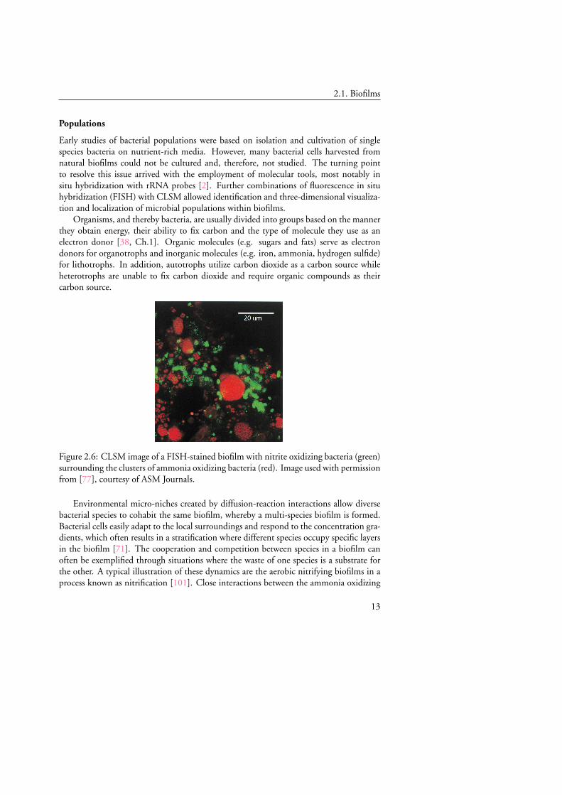
Figure 2.6: CLSM image of a FISH-stained biofilm with nitrite oxidizing bacteria (green)surrounding the clusters of ammonia oxidizing bacteria (red). Image used with permissionfrom [77], courtesy of ASM Journals.
Environmental micro-niches created by diffusion-reaction interactions allow diversebacterial species to cohabit the same biofilm, whereby a multi-species biofilm is formed.Bacterial cells easily adapt to the local surroundings and respond to the concentration gra-dients, which often results in a stratification where different species occupy specific layersin the biofilm [71]. The cooperation and competition between species in a biofilm canoften be exemplified through situations where the waste of one species is a substrate forthe other. A typical illustration of these dynamics are the aerobic nitrifying biofilms in aprocess known as nitrification [101]. Close interactions between the ammonia oxidizing
13

CHAPTER 2. Biofilms in wastewater treatment
bacteria (AOB) and the nitrite oxidizing bacteria (NOB) arise as a result of the depen-dence of NOB on AOB for substrate supply, i.e. AOB convert ammonia to nitrite whichis further converted to nitrate by the NOB. These interactions often lead to small clus-ters of nitrite oxidizing bacteria being close to or surrounding large clusters of ammoniaoxidizing bacteria, interspersed throughout the biofilm [77, 100], instead of exhibiting adistinct stratification, see Figure 2.6.
2.1.2 Harmful and beneficial biofilms
Bacterial biofilms can play both beneficial and detrimental roles in their environment de-pending on whether their formation is controlled or unintentional [11]. A strong moti-vation for research into biofilms has been their persistence and resistance to antimicrobialagents which cause severe medical effects and pose problems in the public health [40].However, recent advances in biofilm research [96] are opening doors toward utilizingbacterial biofilms commercially in the industrial production of chemicals.
Harmful biofilms
Over the years, clinical and public health microbiologists have studied numerous infec-tious diseases from a biofilm perspective. Medical device-associated infections were firstobserved in the early 1980s through detection of bacteria deposited on the surface ofindwelling devices and were the first clinical infections where a correlation to biofilmswas identified [26, 40]. Microorganisms contaminate medical devices and form singleor multi-species biofilms, which subsequently cause severe infections in the human host.Due to inherent biofilm resistance to antimicrobial agents these infections are very dif-ficult to cure [19]. Among the many examples of devices, which in association withbiofilms are known to cause infections [19], urinary catheters, sutures, contact lenses,central venous catheters and mechanical heart valves can be mentioned.
Microorganisms may also form biofilms on damaged human tissue and cause chronicinfections. A common ailment is dental plaque, a biofilm found on tooth surfaces. Dentalplaque is formed regularly in healthy persons, but may alter its microflora to contain morecariogenic strains, which can rapidly metabolize dietary sugars to acid, decreasing the localpH [64]. If left untreated, the biofilms can cause infection, tooth demineralization andtooth loss. The advantage of the easy biofilm accessibility is the possibility to mechanicallyremove biofilms through toothbrushing.
The unwanted deposition and growth of biofilms does not only cause problems inrelation to human health, it is also a common disturbance in water and industrial sys-tems where it is referred to as biofouling [32]. The phenomenon is characterized by thedevelopment of a biofilm which interferes with the proper operation of a water pipe orreactor. Bacteria are always present in the liquid phase of water systems and may uti-lize nutrients available in the water for biomass production, why it is difficult to preventbiofilm formation. A typical example of surfaces that are predisposed to biofouling are
14
2.1. Biofilms
ship hulls. Colonized surfaces can significantly reduce the speed of ships, thereby in-creasing fuel costs. Furthermore, microbially influenced corrosion (MIC), a broad termfor mechanisms by which biofilms affect corrosion of metals, is a serious problem withwidespread effects throughout our society. So far only a few mechanisms have been fullydescribed and quantified, among which the corrosion by sulfate-reducing bacteria is themost known example [58].
Beneficial biofilms
The most successful example of the benefit of biofilms is their ability to remove unwantedcompounds from wastewater in order to safely release the treated water back into the en-vironment. Bacteria have long been used in the biological treatment of wastewater inremoval of organic matter, phosphorous and nitrogen [72]. The biological treatmentincorporates various biofilm-forming bacteria that feed on nutrients present in the wa-ter. They produce compounds that are either further degraded by other bacteria or ina secondary treatment, or that can safely be released into a receiving water body. Somecompounds, like phosphorous, are only taken up by the bacteria without conversion andmoved from the water phase to the biomass.
In the field of bioremediation, a process in which microorganisms are employed in-stead of physicochemical methods to remove pollutants, the usefulness of biofilms is wellestablished. One of the advantages of biological decontamination is the rare productionof toxic intermediates [82], which otherwise tend to persist in the environment, enterthe food web and act as mutagenic or carcinogenic agents on mammals. Recent develop-ments of biofilms in wastewater bioreactors involve bioremediation of heavy metals likezinc, copper and nickel.
2.1.3 Attachment and detachment
The life cycle of a biofilm starts with the arrival of bacteria and ends with their depar-ture, i.e. the processes attachment and detachment as depicted in Figure 2.1. Particularattention has been given to biofilm attachment from a human health perspective wherebiofilm formation is undesired [25]. On the other hand, detachment is considered tobe an important factor in the field of wastewater treatment where stable biofilms serve apurpose [60]. In terms of nomenclature, both attachment and detachment are very broadterms, encompassing several processes.
Attachment
Several factors are assumed to be involved in the initial attachment of bacterial cells toa surface. Among those are mass transport, conditioning of the surface, hydrophobic-ity, surface charge and roughness [79]. Organic and inorganic molecules, along withthe bacteria, are transported to the surface and accumulate at the solid-liquid interface,
15

CHAPTER 2. Biofilms in wastewater treatment
constituting what is commonly known as a conditioning film [57]. The film containsa higher concentration of nutrients compared to the bulk liquid, with physiochemicalproperties that differ from the original unaltered surface [99].
Essentially, bacterial adhesion can be divided into two steps: reversible and irreversibleattachment [79]. The former incorporates the transport of bacteria close enough to thesurface to allow initial interaction between cells and (conditioned) surfaces. In this stepbacterial cells are able to leave the biofilm and can be easily removed by rinsing, etc. Thesecond step of adhesion involves production of EPS that binds firmly to the surface, en-tering an irreversible mode of attachment [27]. In this stage, bacteria cannot be removedwithout physical or chemical intervention, e.g. scrubbing or chemical cleaners.
Bacterial cells may also attach to the surface of a developed biofilm, a process which,however, is poorly understood. Knowledge about the mechanisms of biofilm formationplays a significant role in research about detrimental biofilms, as discussed in Section2.1.2. Attachment is also crucial in wastewater treatment applications where suspendedbiomass and biofilms are present in the same reactor and an exchange of biomass is ob-served, see Section 3.2.3.
Detachment
The final stage of the biofilm development involves active and passive loss of cells to thebulk liquid, either individually or in clusters. Detachment is a complex phenomenon,representing several different mechanisms and factors that cause biomass loss, see Figure2.7. Overall, it is a process of great importance that regulates biomass accumulation,production of suspended solids and biological survival strategies [37].
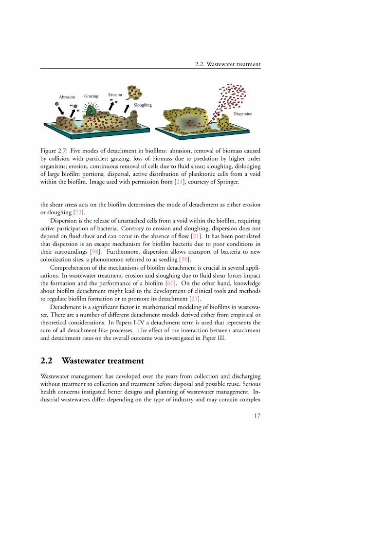
Generally, detachment is divided into five categories of processes [50, 69]: (i) abra-sion, (ii) grazing, (iii) erosion, (iv) sloughing and (v) dispersion. Grazing and abrasion arepassive processes, erosion and sloughing can be both active and passive, whereas disper-sion is always an active removal of cells, which involves mechanisms that are initiated bythe bacteria themselves. The processes are not exclusive, i.e. several modes of detachmentcan occur within the same biofilm.
Abrasion and erosion are the release of cells or small portions of the biofilm, but differin mechanism [21]. Abrasion is caused by collision with submerged particles in the bulkliquid [36]. On the other hand, erosion is caused by fluid shear in a flowing system withbiomass loss occurring when shear forces exceed the cohesiveness of the biofilm [109].
In grazing, higher order organisms cause removal of biomass through predation onbacteria in the biofilm. This process is poorly understood, but is believed to be an impor-tant factor controlling biofilm dynamics [46, 80].
Sloughing involves detachment of large intact portions of the biofilm in discreteevents, at times removing entire segments of biofilm from the substratum. Studies haveshown that local hydrodynamic conditions in relation to biofilm structure trigger biofilmdetachment, where an increase in flow velocity causes an increased amount of detachmentfrom the biofilm that is affected by the shear forces [63, 112]. The local angle at which
16
2.2. Wastewater treatment
Dispersion
Abrasion Grazing Erosion
Sloughing
Figure 2.7: Five modes of detachment in biofilms: abrasion, removal of biomass causedby collision with particles; grazing, loss of biomass due to predation by higher orderorganisms; erosion, continuous removal of cells due to fluid shear; sloughing, dislodgingof large biofilm portions; dispersal, active distribution of planktonic cells from a voidwithin the biofilm. Image used with permission from [21], courtesy of Springer.
the shear stress acts on the biofilm determines the mode of detachment as either erosionor sloughing [73].
Dispersion is the release of unattached cells from a void within the biofilm, requiringactive participation of bacteria. Contrary to erosion and sloughing, dispersion does notdepend on fluid shear and can occur in the absence of flow [21]. It has been postulatedthat dispersion is an escape mechanism for biofilm bacteria due to poor conditions intheir surroundings [98]. Furthermore, dispersion allows transport of bacteria to newcolonization sites, a phenomenon referred to as seeding [50].
Comprehension of the mechanisms of biofilm detachment is crucial in several appli-cations. In wastewater treatment, erosion and sloughing due to fluid shear forces impactthe formation and the performance of a biofilm [60]. On the other hand, knowledgeabout biofilm detachment might lead to the development of clinical tools and methodsto regulate biofilm formation or to promote its detachment [21].
Detachment is a significant factor in mathematical modeling of biofilms in wastewa-ter. There are a number of different detachment models derived either from empirical ortheoretical considerations. In Papers I-IV a detachment term is used that represents thesum of all detachment-like processes. The effect of the interaction between attachmentand detachment rates on the overall outcome was investigated in Paper III.
2.2 Wastewater treatment
Wastewater management has developed over the years from collection and dischargingwithout treatment to collection and treatment before disposal and possible reuse. Serioushealth concerns instigated better designs and planning of wastewater management. In-dustrial wastewaters differ depending on the type of industry and may contain complex
17

CHAPTER 2. Biofilms in wastewater treatment
or toxic substances, while municipal wastewater mostly consists of organic matter andnutrients in either solid or soluble form. This thesis will exclusively address municipalwastewater treatment.
The objectives of (municipal) wastewater treatment are to remove contaminants and,thereby, to produce a safe effluent which can be discharged into receiving water bodieswithout harming the environment. Generally, wastewater treatment is performed in threemajor steps: primary, secondary and tertiary treatment [91]. Primary treatment typicallyconsists of screening and settling where large particles and objects are removed and heavyand light solids are separated from the fluid. It is followed by a secondary treatmentin which a biological process takes place where microorganisms remove suspended anddissolved organic matter, as mentioned in Section 2.1.2. The increased knowledge of theeffects of chemicals and toxic compounds has resulted in the need for a tertiary treatment,which can be for example chemical or biological. Typically it involves disinfection, odorcontrol and removal of the nutrients nitrogen and phosphorous.
Microorganisms are used in the second step to remove organic matter from the fluidmost often in a process commonly known as activated sludge. The process requires anaerated reactor, a settling tank, sludge recirculation and removal of excess sludge [111].The biomass is kept in suspension in an aerated reactor where the biochemical reactionstake place. It is followed by a settling tank, in which the biomass sinks to the bottom,separating it from the clarified effluent. The settled biomass is mainly recirculated tothe aerated reactor, to preserve a high concentration of biomass, which otherwise wouldbe discharged. The remaining part, excess sludge, is removed and further treated in thesludge treatment stage.
Due to eutrophication, i.e. the over-enrichment of receiving water sources with min-eral nutrients [15], the tertiary treatment stage involves removal of nutrients. Increasedamounts of phosphorus (P) and nitrogen (N) in a lake or sea enhance the proliferationof algae and bacteria. This in turn leads to oxygen-free bottom waters due to high res-piration by the biomass, thereby causing loss of fish and other aquatic animals naturallyoccurring in the water. Although eutrophication is a natural process, the superfluous ad-dition of nutrients aggravates the development, wherefore discharge of P and N has beenincreasingly regulated in wastewater treatment. Removal of P and N is added as a tertiarytreatment stage, with the latter discussed in more detail in Section 2.2.2.
Bacteria in the form of activated sludge or biofilms are not only used in secondarytreatment, but are also present in tertiary treatment. They can be used for removal of bothphosphorus and nitrogen. Biofilm processes and the reactor setups differ from those ofactivated sludge. Instead of being suspended in the liquid, biofilm biomass is attached to asurface that is submerged in the liquid. Therefore, there is no need for settling and sludgerecirculation. Biofilms provide means for slow growing bacteria to grow and remainin a reactor. Many different biofilm reactors are available in contemporary wastewaterengineering, from fixed bed reactors such as the trickling filter, submerged fixed-filmreactors such as the rotating biological contactor to fluidized bed reactors such as the
18

2.2. Wastewater treatment
upflow sludge blanket [66]. Section 2.2.1 will cover the Moving Bed Biofilm Reactor, inwhich biofilms are attached to suspended media that move freely in the liquid.
2.2.1 Moving Bed Biofilm Reactor
The moving bed biofilm reactor (MBBR) process was developed in Norway in the late1980s to overcome the problems of existing biofilm systems used in wastewater treat-ment, while implementing the best features of the activated sludge process [74]. It hassince become a common process used in treatment plants worldwide, either as an addedtreatment unit in an existing plant or as an integral part of the plant.
a) Aeration b) Carriers c) Mechanical mixing
Figure 2.8: a) Aerobic tank with suspended carriers and aeration from the bottom. b) Dif-ferent kinds of carriers. c) Anoxic tank with suspended carriers and mechanical mixing.Images used with permission, courtesy of AnoxKaldnes, Sweden.
In an MBBR the biomass is attached to carriers (Figure 2.8b) that are suspended inthe water. The carriers are mixed in the liquid either through rising coarse air bubbles dueto aeration (Figure 2.8a) or through mechanical mixing in oxygen-free processes (Figure2.8c), and kept from leaving the reactor by a sieve. The carriers are designed with thebiofilm area as the key parameter. A reactor can be filled with varying amounts of carriers,although the standard filling fraction is 40 to 65%. Here, the filling fraction is the volumeof carrier elements relative to the water volume of the reactor in which they are suspended.
The MBBR process requires no sludge recirculation nor a large sedimentation tank,which gives it a great advantage over the activated sludge process [95]. Furthermore, it iseasily managed and can often be set up using existing tanks, thereby being cost effective.The process is compact due to high concentration of biomass which can be differentiatedwith respect to bacterial species. However, the MBBR has increased operational costsdue to larger power requirements for aeration/mixing, in particular to maintain activityduring low loading phases, and a higher initial cost of carrier acquisition. Moreover, theeffluent from an MBBR must be treated in order to remove the sloughed off biofilm fromthe treated water. This can be achieved through a variety of biomass separation methodssuch as sedimentation, flotation or filtration after the MBBR [75, 76]. The MBBR ef-fluent contains several types of particulates, among which the sloughed off biomass and
19

CHAPTER 2. Biofilms in wastewater treatment
the influent particulate matter are the most significant [47]. Compared with a standardactivated sludge reactor there is approximately ten times less suspended biomass to beseparated in the MBBR effluent, but still enough to require treatment. Hence, there isalways a certain amount of suspended biomass present even in pure MBBR systems. TheMBBR process is used in the mathematical models throughout this thesis, with particularfocus on the interaction between attached and suspended biomass in Papers I, III and IV.
2.2.2 Nitrification
The agricultural development during recent years, with emphasis on fertilization of crop-land, has increased the need for nutrient removal. High nitrogen loads promote eutroph-ication, which is harmful for the environment. Nitrogen is, therefore, removed fromwastewater through sequential processes called nitrification and denitrification, whichconvert ammonium-nitrogen from the wastewater to nitrogen gas and in lesser amountsnitrous oxide, safe for release into the atmosphere. An additional nitrogen pathway existsthrough the process anammox (anaerobic ammonium oxidation), which, however, willnot be discussed in this thesis.
Nitrification is a process in which ammonium (NH+4 ) is sequentially oxidized to
nitrate (NO−3 ) with the intermediate component nitrite (NO−2 ) [59]. The chemicalreactions are expressed as:
(i) : NH+4 + 1.5O2 → NO−2 + 2H+ + H2O (2.1)
(ii) : NO−2 + 0.5O2 → NO−3 (2.2)
where the first reaction (i) is performed by ammonium oxidizing bacteria (AOB) and thesecond reaction (ii) by nitrite oxidizing bacteria (NOB), i.e.
NH+4
AOB−−→ NO−2NOB−−−→ NO−3 . (2.3)
These bacteria use nitrogen as an electron donor, oxygen as an electron acceptor and fixcarbon from carbon dioxide, wherefore they are classified as chemolithoautotrophs, seeSection 2.1.1. Nitrification is an aerobic process, i.e. requires oxygen for the reactions totake place, why maintaining a high concentration of dissolved oxygen is a crucial task. Ifno other inhibitions are present, the first reaction (i) is the rate-limiting step of the overallconversion from ammonium to nitrate [122].
The two most common bacterial genera of AOB are the Nitrosomonas and Nitrosospira[55]. For NOB, the two most common genera are the Nitrobacter and Nitrospira [12].AOB and NOB co-habit the same space within a biofilm and benefit from the physicalproximity during the nitrification process [83], previously discussed in relation to Figure2.6. NOB consume the product that is the outcome of the first reaction performed byAOB, thereby relieving the latter from toxic waste. Optimal temperatures for growth of
20
2.2. Wastewater treatment
pure cultures were shown to be 35◦C and 38◦C for AOB and NOB, respectively [39].The specific growth rates for AOB are higher than for NOB at temperatures above 15◦C,while the opposite occurs at lower temperatures [42]. The MBBR processes used in PapersII and III are assumed to operate at a temperature of 10◦C, to represent nitrification ina colder climate. The chosen temperature is far from the optimal temperature range,bringing about slower growth rates for both species and an advantage for NOB overAOB, resulting in different interactions than would have occurred at room temperatures.In comparison with heterotrophic bacteria that consume organic matter, the growth ratesfor AOB and NOB are much slower. The nitrifiers, therefore, benefit from the protectedsurfaces on the carriers in an MBBR, which allows them to form a stable biomass withoutbeing exposed to the risk of washout. Heterotrophic biomass, on the other hand, worksvery well in an activated sludge process.
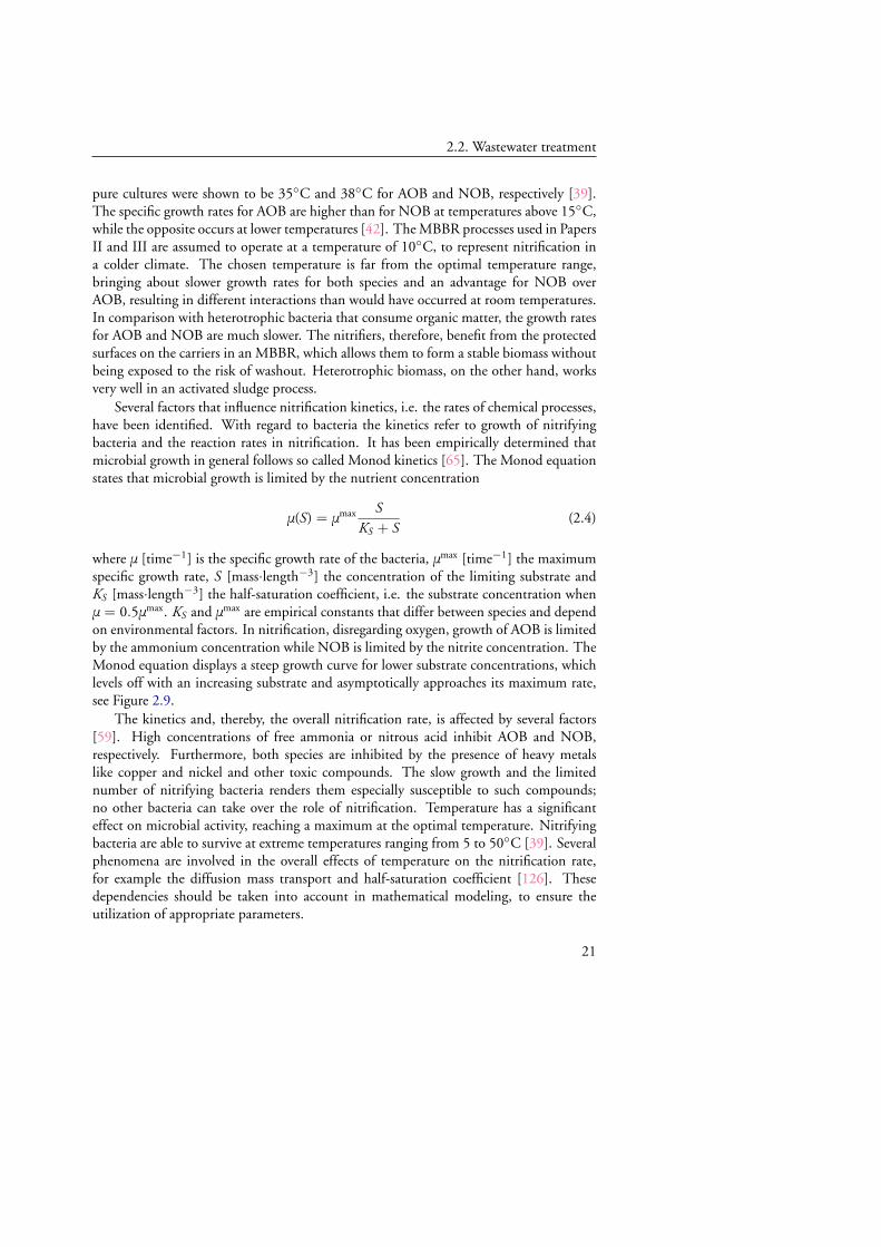
Several factors that influence nitrification kinetics, i.e. the rates of chemical processes,have been identified. With regard to bacteria the kinetics refer to growth of nitrifyingbacteria and the reaction rates in nitrification. It has been empirically determined thatmicrobial growth in general follows so called Monod kinetics [65]. The Monod equationstates that microbial growth is limited by the nutrient concentration
μ(S) = μmax SKS + S
(2.4)
where μ [time−1] is the specific growth rate of the bacteria, μmax [time−1] the maximumspecific growth rate, S [mass·length−3] the concentration of the limiting substrate andKS [mass·length−3] the half-saturation coefficient, i.e. the substrate concentration whenμ = 0.5μmax. KS and μmax are empirical constants that differ between species and dependon environmental factors. In nitrification, disregarding oxygen, growth of AOB is limitedby the ammonium concentration while NOB is limited by the nitrite concentration. TheMonod equation displays a steep growth curve for lower substrate concentrations, whichlevels off with an increasing substrate and asymptotically approaches its maximum rate,see Figure 2.9.
The kinetics and, thereby, the overall nitrification rate, is affected by several factors[59]. High concentrations of free ammonia or nitrous acid inhibit AOB and NOB,respectively. Furthermore, both species are inhibited by the presence of heavy metalslike copper and nickel and other toxic compounds. The slow growth and the limitednumber of nitrifying bacteria renders them especially susceptible to such compounds;no other bacteria can take over the role of nitrification. Temperature has a significanteffect on microbial activity, reaching a maximum at the optimal temperature. Nitrifyingbacteria are able to survive at extreme temperatures ranging from 5 to 50◦C [39]. Severalphenomena are involved in the overall effects of temperature on the nitrification rate,for example the diffusion mass transport and half-saturation coefficient [126]. Thesedependencies should be taken into account in mathematical modeling, to ensure theutilization of appropriate parameters.
21

CHAPTER 2. Biofilms in wastewater treatment
S
µ(S
)
KS
0.5 µmax
µmax
Figure 2.9: The Monod equation for microbial growth rate μ(S) on substrate S at amaximum specific growth rate μmax and a half-saturation coefficient KS .
Apart from substrate availability, it is also crucial that a high level of dissolved oxygen(DO) is present in a nitrification reactor. The nitrifiers are obligate aerobes and requirethe presence of oxygen for growth. Low DO will limit the nitrification rate, particularly inbiofilm applications where diffusion of oxygen into the biofilm will pose a second obstaclefor oxygen availability. In general, it is believed that a DO level below 2 mg/l is limitingfor nitrifying bacteria in biofilms [13]. Due to diffusion and reaction oxygen may becomelimiting in the depths of a biofilm even though the bulk concentration has a sufficientlevel of DO. The affinity for oxygen differs between AOB and NOB, where the lattergenerally requires a higher DO concentration for microbial growth [83]. In wastewatertreatment biofilm reactors there is a possibility for organic matter to enter the nitrificationreactor. If organic matter is present it will serve as a substrate for heterotrophic bacteriawhich will compete for oxygen and space with nitrifying bacteria [13]. A heterotrophiclayer may form on top of the nitrifiers in the biofilm and limit the oxygen penetration. Aslong as the nitrifiers are reached by a high enough oxygen concentration they will establishthemselves and remain in the depths of the biofilm [35]. In these cases, the heterotrophiclayer is often beneficial to the nitrifiers because it protects them from detachment.
22
Chapter 3
Biofilm modeling
3.1 Mathematical models in biology
Fibonacci (1175-1250) is often named as a pioneer in mathematical biology due to hisnumber series that aimed to represent the reproduction of rabbits [54]. The series, inwhich the next number is the sum of its two predecessors, has later also been found inother parts of nature, for example in the growth of certain shells and most notably inthe distribution of seeds in a sunflower. Over the centuries people have shown interestin understanding and deciphering our surroundings. The field of biology encompassesall living organisms, ranging from studies of among others plants and animals, cells andmolecules to evolution, populations and genetics. The resulting catalog of mathematicalmodels in biology therefore displays a similar range from small scale to large scale, sim-ple to complex, linear to nonlinear etc. Examples of biological phenomena described bymathematical models include the predator-prey model of Lotka and Volterra, infectiousdisease models, tumor cell growth models and fishery management models [70]. A com-mon misconception about mathematical models is that they are supposed to explain anddepict a phenomenon in detail, reproducing the real life behavior to its fullest. This is,however, not the case. Mathematical models are a helpful tool that through simplificationof the observed phenomenon can bring the theoretical or experimental work forward. Ithas been claimed that, more often than not, the mathematical model will predict biolog-ically infeasible results [29, Ch.3]. But the subsequent investigation of the causes thereofmay shed light onto the phenomenon itself as well as pose questions which will point theresearchers in a new direction. The most fundamental processes in biofilms are microbialgrowth and mass transfer. In the next two sections the mathematical framework for thesetwo concepts will be briefly reviewed, which will be needed later on.
23

CHAPTER 3. Biofilm modeling
3.1.1 Chemostat
In many subfields of biology it is common to study the population growth of organisms.In microbiology it is usually done through an experiment where microorganisms are sus-pended in a nutrient-rich liquid in which they proliferate [29]. Their growth is typicallyobserved through an increase in volume and density. Depending on the circumstancesduring the experiment most microorganisms show a growth that can be characterized aslogistic or exponential. A more realistic type of bacterial growth is the saturated nutri-ent consumption rate, where the growth rates are nutrient-dependent. Monod kinetics(previously discussed in Sec. 2.2.2), described by the equation μ(S) = μmax S
KS+S in (2.4),shows a growth rate that is proportional to the substrate concentration if nutrient avail-ability is limited and levels off to a constant value if nutrients are available in abundance,see Figure 2.9.
Inflow
Outflow
Figure 3.1: The chemostat with stirring and continuous inflow and outflow.
A bioreactor with stirring and continuous inflow and outflow is called a chemo-stat [102]. The chemostat provides a dynamic system for population studies and isextensively used in laboratory experiments. Nutrient is continuously supplied throughthe inflow and continuously removed through the outflow, while the liquid volume inthe reactor is kept constant, see Figure 3.1. Various microorganisms, with concentra-tions xi(t) [mass·length−3] for the i = 1, . . . , n species, are suspended in the reactor.Let Q [length3·time−1] denote the flow rate, V [length3] the reactor volume and S0
[mass·length−3] the concentration of the input nutrient. It is assumed that all compo-nents that are necessary for bacterial growth are in excess except one limiting nutrient,denoted by S(t). The flow rate Q and the input concentration S0 are kept constant alongwith all other parameters that affect microbial growth. The rates of change for the bacteria
24
3.1. Mathematical models in biology
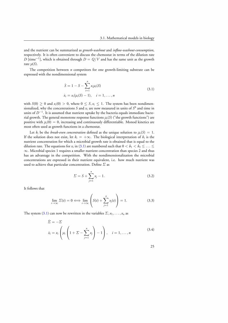
and the nutrient can be summarized as growth-washout and inflow-washout-consumption,respectively. It is often convenient to discuss the chemostat in terms of the dilution rateD [time−1], which is obtained through D = Q/V and has the same unit as the growthrate μ(S).
The competition between n competitors for one growth-limiting substrate can beexpressed with the nondimensional system
S = 1− S −n∑
i=1
xiμi(S)
xi = xi(μi(S)− 1), i = 1, . . . , n
(3.1)
with S(0) ≥ 0 and xi(0) > 0, where 0 ≤ S, xi ≤ 1. The system has been nondimen-sionalized, why the concentrations S and xi are now measured in units of S0 and time inunits of D−1. It is assumed that nutrient uptake by the bacteria equals immediate bacte-rial growth. The general monotone response functions μi(S) ("the growth functions") arepositive with μi(0) = 0, increasing and continuously differentiable. Monod kinetics aremost often used as growth functions in a chemostat.
Let bi be the break-even concentration defined as the unique solution to μi(S) = 1.If the solution does not exist, let bi = +∞. The biological interpretation of bi is thenutrient concentration for which a microbial growth rate is obtained that is equal to thedilution rate. The equations for xi in (3.1) are numbered such that 0 < b1 < b2 ≤ . . . ≤∞. Microbial species 1 requires a smaller nutrient concentration than species 2 and thushas an advantage in the competition. With the nondimensionalization the microbialconcentrations are expressed in their nutrient equivalent, i.e. how much nutrient wasused to achieve that particular concentration. Define Σ as
Σ = S +
n∑j=1
xj − 1. (3.2)
It follows that
limt→∞
Σ(t) = 0⇐⇒ limt→∞
S(t) +
n∑j=1
xj(t)
= 1. (3.3)
The system (3.1) can now be rewritten in the variables Σ , x1, . . . , xn as
Σ = −Σ
xi = xi
μi
1 + Σ −n∑
j=1
xj
− 1
, i = 1, . . . , n(3.4)
25

CHAPTER 3. Biofilm modeling
Solutions of (3.1) and (3.4) exist and are non-negative and bounded. Using (3.3) andconsidering the system (3.4) restricted to the invariant hyperplane Σ = 0, the system canbe simplified to
xi = xi
μi
1−n∑
j=1
xj
− 1
, i = 1, . . . , n (3.5)
on the positively invariant domain Ω ={
x ∈ Rn+ :∑n
j=1 xj ≤ 1}
with xi(0) > 0.
All microbial competitors with a break-even concentration that is equal to or exceedsthe nutrient concentration in the reactor, i.e. bi ≥ 1, are deemed inadequate as theywill eventually be eliminated from the reactor. Thus, only adequate competitors with0 < bi < 1 are considered. Let x1 be an adequate competitor and let
E1 = (1− b1, 0, 0, . . . , 0) (3.6)
be the equilibrium point for (x1, . . . , xn) in (3.5) at which only species x1 survives. Con-sideration of equilibrium points for other adequate species for some j ≥ 2 is not necessaryfor the statement of the main result about competitive exclusion.
Theorem 3.1.1. Let x(t) be a solution to (3.5) in Ω for which x1(0) > 0. Then
limt→∞
x(t) = E1. (3.7)
The theorem states that the microbial species with the smallest break-even concen-tration will outcompete all other species in a chemostat and remain alone in the re-actor. Lyapunov functions and the LaSalle corollary of Lyapunov stability theory are
used to prove the theorem. By defining the sets ΔA ={
x ∈ Ω :∑
j xj = 1− b1
},
ΔB ={
x ∈ Ω :∑
j xj < 1− b1
}and ΔC =
{x ∈ Ω :
∑j xj > 1− b1
}, it is shown
that a solution that starts in ΔC either moves to ΔB or remains in ΔC and converges toE1. Solutions inΔB remain in the set and converge to E1.
Theorem 3.1.1 presents a mathematical result which has subsequently been confirmedwith biological experiments. In a proper chemostat setting with several species compet-ing for one nutrient, the microbial species with the smallest break-even concentrationwill eliminate all other species from the reactor. The result is used by microbiologiststo design chemostat experiments. The chemostat is often used for bacterial enrichmentand harvesting [29, Ch.4]. Further applications include steady state analysis of differentorganisms and interactions and competition between populations. However, the resultrests on the assumption that the growth of each competitor is described by a monotonefunction and that there is no interaction between the competitors. The principle of com-
26

3.1. Mathematical models in biology
petitive exclusion does not hold if one species has a (non-competitive) growth advantageover the other [31], if there is a direct exchange of biomass between the species, or if oneof the species is protected from washout. The latter two aspects need to be considered inbiofilm reactors with suspended growth, which requires an extension of the above theory.
3.1.2 Conservation of mass, diffusion and transport
The principle of mass conservation states that all mass/matter/energy in an isolated systemis conserved. The mass conservation equation can be derived by use of the divergencetheorem [24, Ch.2].
Let V ∈ Rd , d = 1, 2, 3, denote the fixed control volume containing a substancewith concentration C (t, x) and let ∂V denote the closed surface boundary of V . Themass M (t) of the substance contained in V is the volume integral
M (t) =
˚
V
C (t, x) dV (3.8)
where dV is the differential element of the volume V . Conservation of mass implies that
rate of change of M in V = production in V︸ ︷︷ ︸source
− outflux through ∂V︸ ︷︷ ︸sink
(3.9)
which is mathematically expressed as
dMdt
=
˚
V
R dV −‹
∂V
J · n dS (3.10)
where R is the local production rate and where the second term on the right hand side is asurface integral of the total flux J of the substance in the direction of the outward normaln through the differential surface elements dS on ∂V . Applying the divergence theoremthe surface integral can be converted into a volume integral
‹
∂V
J · n dS =
˚
V
div J dV . (3.11)
Substituting (3.11) into (3.10) and using (3.8) leads to
ddt
˚
V
C (t, x) dV =dMdt
=
˚
V
R dV −˚
V
div J dV (3.12)
27

CHAPTER 3. Biofilm modeling
which can be rewritten under one integral as
˚
V
(∂Cdt− R + div J
)dV = 0. (3.13)
Since the equality in Equation (3.13) has to hold for any arbitrary volume V it followsthat
∂Cdt− R + div J = 0. (3.14)
The conservation law is expressed in its integral form in (3.13) and in its differential formin (3.14).
The expression for the flux J can be adapted to the situation at hand. An importanttransport process for particles is diffusion, in which the random and irregular motionof individuals in a group results in a movement on a macroscopic level [70]. Diffusiontransports matter down the concentration slope, i.e. from high to low concentration, alsoknown as Fick’s first law. The law states that the flux J is proportional to the gradient ofthe concentration C
J = −Dc∇C (3.15)
where Dc [length2·time−1] is the diffusion coefficient that measures the efficiency of par-ticle dispersal and ∇ denotes the gradient. Diffusion is in general a fast process locally,but an extremely slow process on longer distances [29, Ch.9]. The diffusion-reactionequation follows from (3.14) and (3.15):
∂C∂t
= R −∇ · (−Dc∇C ) (3.16)
where ∇· = div, which becomes
∂C∂t
= R + Dc∇2C (3.17)
if Dc is constant. The equation is a semilinear parabolic partial differential equation andrequires appropriate initial and boundary conditions.
Another mode of particle transport, advection (transport of particles in a fluid by thefluid flow), was discussed in Section 2.1.1. Advective flux can be described by uC whereu [length·time−1] is the average flow velocity of the liquid. Let the flux J denote bothdiffusive and advective flux
J = −Dc∇C + uC (3.18)
which, when substituted into (3.14), gives the general transport equation, also known as
28

3.2. Biofilm models
the advection-diffusion-reaction equation
∂C∂t
= R + Dc∇2C −∇(uC ). (3.19)
The transport equation, or versions thereof, will be discussed in Section 3.2 as a suitablerepresentation of biofilm development.
3.2 Biofilm models
3.2.1 Overview
Before the breakthrough of new tools like the confocal laser scanning microscope and themicroelectrode measurements that enabled detailed observation, biofilms were roughlyperceived as homogeneous layers of biomass that could grow by consuming a substratedelivered with the bulk liquid. Biofilm models are changing with advances in microbiol-ogy and with the increase in possible applications. Even within a given application there isan evolution of the model as we learn more about the biofilm system and its environmenton a physical, chemical and biological level [53]. Still, there are several obstacles thatneed to be tackled, like the influence of macroscale physical factors on biofilm composi-tion and structure. The main difficulty is to incorporate all processes of such a complexsystem, on a wide variety of time and length scales into an exhaustive and understandablemodel [113]. For example, despite the increasing knowledge about biofilms there is a lackof understanding of the crucial processes attachment and detachment of biomass, whichgovern much of the development of a biofilm. The complexity of these processes is rarelyvisible in the mathematical models where an ad hoc technique has been used in mostmodels to describe detachment by a rate proportional to the square of the biofilm height.
The varying levels of biofilm description are also apparent in mathematical modelswhich contain different levels of complexity. The most significant distinctions are madebetween one-dimensional (1D) and two- and three-dimensional models (2D/3D), dy-namic and steady state models, and single species/substrate and multi-species/-substratemodels. An increased modeling and process complexity implies an increased mathemat-ical and numerical complexity which makes the choice of model a trade-off decision.Biofilm models in wastewater engineering were comprehensively compared in [114],where it was found that numerical 1D models describe the wastewater process well andare much easier to work with than 2D/3D models. The multi-dimensional models re-quire numerical treatment and large computing power while the 1D models often allowfor mathematical analysis. The focus of this thesis will be on the one-dimensional biofilmmodel, introduced in detail in the next section.
29
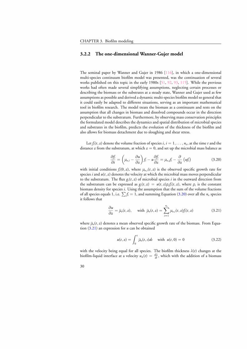
CHAPTER 3. Biofilm modeling
3.2.2 The one-dimensional Wanner-Gujer model
The seminal paper by Wanner and Gujer in 1986 [116], in which a one-dimensionalmulti-species continuum biofilm model was presented, was the continuation of severalworks published on this topic in the early 1980s [51, 92, 93, 115]. While the previousworks had often made several simplifying assumptions, neglecting certain processes ordescribing the biomass or the substrates at a steady state, Wanner and Gujer used as fewassumptions as possible and derived a dynamic multi-species biofilm model so general thatit could easily be adapted to different situations, serving as an important mathematicaltool in biofilm research. The model treats the biomass as a continuum and rests on theassumption that all changes in biomass and dissolved compounds occur in the directionperpendicular to the substratum. Furthermore, by observing mass conservation principlesthe formulated model describes the dynamics and spatial distribution of microbial speciesand substrates in the biofilm, predicts the evolution of the thickness of the biofilm andalso allows for biomass detachment due to sloughing and shear stress.
Let fi(t, z) denote the volume fraction of species i, i = 1, . . . , nx , at the time t and thedistance z from the substratum, at which z = 0, and set up the microbial mass balance as
∂fi∂t
=
(μo,i −
∂u∂z
)fi − u
∂fi∂z
= μo,ifi −∂
∂z
(ufi)
(3.20)
with initial conditions fi(0, z), where μo,i(t, z) is the observed specific growth rate forspecies i and u(t, z) denotes the velocity at which the microbial mass moves perpendicularto the substratum. The flux gi(t, z) of microbial species i in the outward direction fromthe substratum can be expressed as gi(t, z) = u(t, z)ρifi(t, z), where ρi is the constantbiomass density for species i. Using the assumption that the sum of the volume fractionsof all species equals 1, i.e.
∑fi = 1, and summing Equation (3.20) over all the nx species
it follows that
∂u∂z
= μo(t, z), with μo(t, z) =
nx∑i=1
μo,i(t, z)fi(t, z) (3.21)
where μo(t, z) denotes a mean observed specific growth rate of the biomass. From Equa-tion (3.21) an expression for u can be obtained
u(t, z) =
ˆ z
0μo(t, s)ds with u(t, 0) = 0 (3.22)
with the velocity being equal for all species. The biofilm thickness λ(t) changes at thebiofilm-liquid interface at a velocity ul(t) = dl
dt , which with the addition of a biomass
30
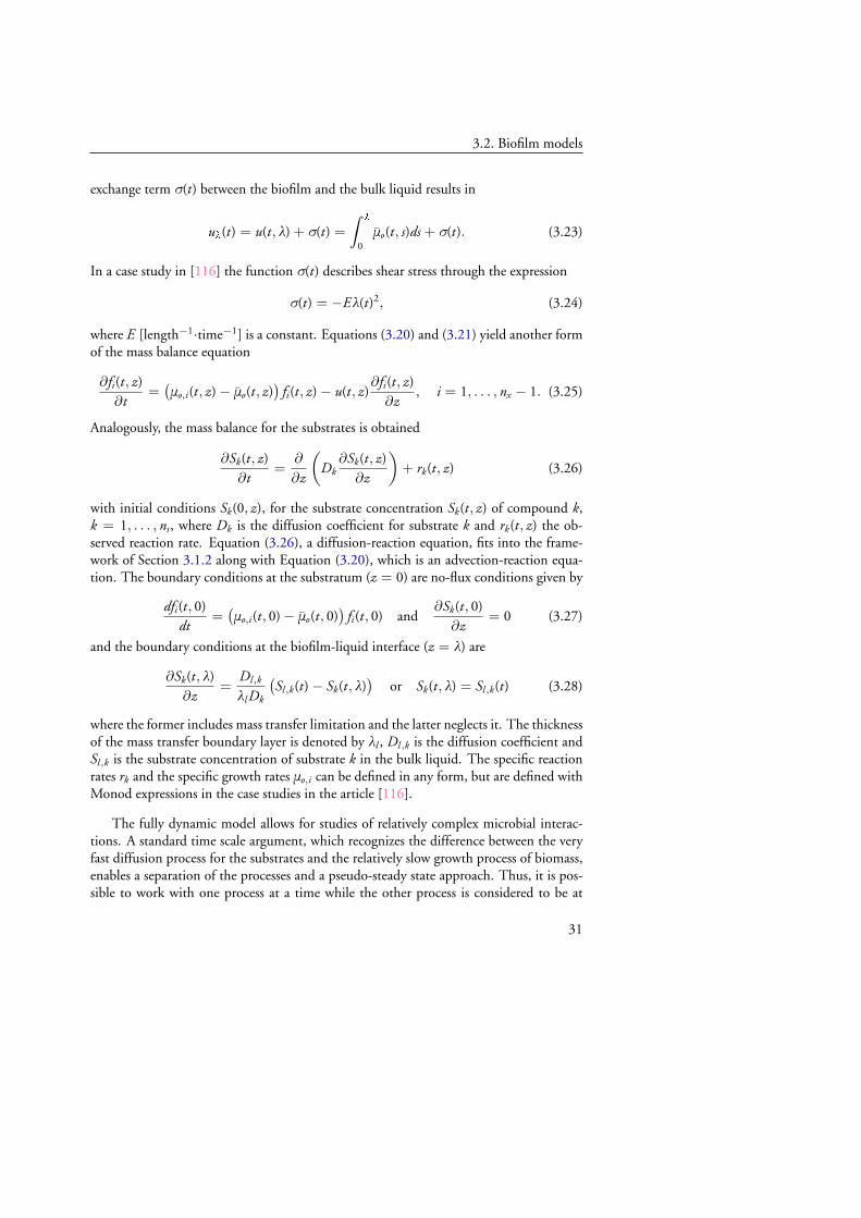
3.2. Biofilm models
exchange term σ(t) between the biofilm and the bulk liquid results in
ul(t) = u(t, λ) + σ(t) =
ˆ l
0μo(t, s)ds + σ(t). (3.23)
In a case study in [116] the function σ(t) describes shear stress through the expression
σ(t) = −Eλ(t)2, (3.24)
where E [length−1·time−1] is a constant. Equations (3.20) and (3.21) yield another formof the mass balance equation
∂fi(t, z)∂t
=(μo,i(t, z)− μo(t, z)
)fi(t, z)− u(t, z)
∂fi(t, z)∂z
, i = 1, . . . , nx − 1. (3.25)
Analogously, the mass balance for the substrates is obtained
∂Sk(t, z)∂t
=∂
∂z
(Dk
∂Sk(t, z)∂z
)+ rk(t, z) (3.26)
with initial conditions Sk(0, z), for the substrate concentration Sk(t, z) of compound k,k = 1, . . . , ns, where Dk is the diffusion coefficient for substrate k and rk(t, z) the ob-served reaction rate. Equation (3.26), a diffusion-reaction equation, fits into the frame-work of Section 3.1.2 along with Equation (3.20), which is an advection-reaction equa-tion. The boundary conditions at the substratum (z = 0) are no-flux conditions given by
dfi(t, 0)dt
=(μo,i(t, 0)− μo(t, 0)
)fi(t, 0) and
∂Sk(t, 0)∂z
= 0 (3.27)
and the boundary conditions at the biofilm-liquid interface (z = λ) are
∂Sk(t, λ)∂z
=Dl,k
λl Dk
(Sl,k(t)− Sk(t, λ)
)or Sk(t, λ) = Sl,k(t) (3.28)
where the former includes mass transfer limitation and the latter neglects it. The thicknessof the mass transfer boundary layer is denoted by λl , Dl,k is the diffusion coefficient andSl,k is the substrate concentration of substrate k in the bulk liquid. The specific reactionrates rk and the specific growth rates μo,i can be defined in any form, but are defined withMonod expressions in the case studies in the article [116].
The fully dynamic model allows for studies of relatively complex microbial interac-tions. A standard time scale argument, which recognizes the difference between the veryfast diffusion process for the substrates and the relatively slow growth process of biomass,enables a separation of the processes and a pseudo-steady state approach. Thus, it is pos-sible to work with one process at a time while the other process is considered to be at
31

CHAPTER 3. Biofilm modeling
a pseudo-steady state. This approach reduces the computational effort, but maintainsaccuracy. Investigation of the biomass volume fractions can reveal a heterogeneous lay-ering within the biofilm with respect to the different species. Wanner and Gujer used aheterotrophic-autotrophic setting in wastewater treatment (where the species both com-pete for oxygen) and numerical simulations to demonstrate the abilities of their model.
Most applications use biofilm models in the context of numerical simulations. Onlya few studies are known where biofilm models have been approached with analyticaltechniques. Existence and properties of solutions and of the corresponding steady-statesolutions of a one-dimensional biofilm model have been addressed in [88, 107]. Furtherextensions to [107] with focus on persisters and antimicrobial treatment were presentedand studied in [14, 108]. In analogy with the study in Paper I, the overall communityproductivity and system equilibria for a one-dimensional biofilm model was investigatedin [52].
3.2.3 Biofilm models in wastewater applications
The state-of-the-art biofilm model in wastewater treatment was introduced in 1996 in[117], which was an extension of the Wanner and Gujer model from [116]. The contin-uum approach and the one-dimensionality of the previous model were maintained whilenew processes and more flexibility was added in order to account for new experimen-tal findings. For example, porosity within the biofilm was included, allowing for liquidphase volume fractions between the biofilm’s particulate components. Furthermore, thenet result of biofilm cell movements within the biofilm was modeled by an effective dif-fusive flux. The model was developed for a wastewater application in which an aerobicheterotrophic-autotrophic biofilm in a completely mixed bulk liquid consumes organicmatter and ammonium. The two species compete for space and oxygen and are governedby the processes growth, inactivation and respiration. Inert matter is formed throughinactivation of active biofilm cells, constituting a third biofilm species.
Implementation of the model in AQUASIM [90] created a template for biofilm mod-els in wastewater treatment, allowing for modifications in order to represent the specificsystems at hand. It is an accessible and valuable tool for understanding biofilm processesand is, therefore, widely used in many different applications. The one-dimensional modelhas also been implemented in many other software packages, e.g. BioWin, GPS-X, Simbaand STOAT, with a comprehensive overview in [7].
Mass transfer and utilization of substrate in an autotrophic biofilm system [45] as wellas growth and decay in an autotrophic-heterotrophic biofilm [44] were investigated exper-imentally with the aim of verifying and improving the model of [117]. A different contextwas presented in [94] where the model was used to describe tolerance of biofilms with re-spect to antibiotics based on the mechanism of slow growth and nutrient limitation. Themodel was also successfully adapted to the wastewater application of nitrification anddenitrification by biofilms growing on sand grains in a sand filter [120]. Others com-
32

3.2. Biofilm models
bined removal of nitrate with removal of phosphorus in a biofilm reactor for enhancedbiological phosphorus removal and investigated diffusion limitation [30]. A more com-plex system was presented in [5] where a mixed-culture biofilm containing autotrophicdenitrifiers, sulfate reducing bacteria and heterotrophs performs oxidized nitrogen, sulfurand selenium removal.
Despite the wide applicability of different software packages there is a limitation onthe dimensionality of the model. One of the main assumptions is that the biofilm isplanar and one-dimensional, which does not suffice for describing a proper biofilm struc-ture. To broaden the understanding of the structure-environment-activity relation it isnecessary to use multi-dimensional models that describe spatial heterogeneity in multipledirections. Pure continuum models like [1] and [28], often extending the work of Wan-ner and Gujer, have been introduced along with other approaches like cellular automata[86] and individual based modeling [84]. While multidimensional models offer morecomplexity and detailed descriptions of the processes, particularly with respect to biofilmstructure [87], they also require greater computational effort and a higher level of inputand control from the user. Moreover, the use of multi-dimensional models is restrictedto very small domains, much smaller than a lab or full scale reactor. The advantages anddisadvantages of simple models will be further discussed in Section 3.2.4.
As biofilms in wastewater treatment are mostly used for nitrogen and phosphorus re-moval, these applications prevail among the biofilm models. Nitrification, i.e. conversionof ammonium to nitrate by autotrophic bacteria, is sometimes combined with organicmatter removal (aerobically by heterotrophic bacteria), denitrification [118] (anoxic con-version of nitrate to nitrogen gas by heterotrophic bacteria) or with the anammox process[41] (anoxic conversion of ammonium and nitrite to nitrogen gas by anammox bacteria).Typically, nitrification is modeled either as a one-step or a two-step process. Wanner andGujer in [116] used the former model in combination with presence of heterotrophicbacteria to account for removal of organic matter, see the stoichiometric matrix in Table3.1. Substrates are denoted by Sk, volume fractions by fi, biomass density by ρi, half-saturation Monod coefficient by K , endogenous respiration constant by b, inactivationconstant by k, maximum specific growth rate by μmax and biomass yield by Y . In theirmodel the ammonium is not converted to anything, it is only consumed and thereby re-moved. For two-step nitrification, where ammonium is converted to nitrite and furtherto nitrate, the autotrophic part in Table 3.1 is divided into several processes for the twospecies AOB and NOB and two more substrates are introduced. An example is givenin Table 3.2 from [10]. The included processes are growth, inactivation and aerobicand anoxic endogenous respiration for the biomass compounds AOB (XAOB) and NOB(XNOB) respectively for the involved dissolved compounds oxygen SO2, ammonium SNH4,nitrite SNO2 and nitrate SNO3. The anoxic reduction factor for endogenous respirationis denoted by η and the production of inert matter XI in endogenous respiration by fXI .By extending nitrification into two steps the model complexity is increased and a morerealistic description of the process is obtained. However, when nitrification is used as a
33

CHAPTER 3. Biofilm modeling
submodule in a larger model it may be desirable to maintain the one-step description inorder to allow for more modules without complicating the model extensively.
It is already apparent that biofilm models contain many parameters and constants,whose number increases with increasing model complexity. In a relatively simple modeldescribed in Table 3.1 there are 16 parameters that need to be determined or chosenfrom literature. Many parameters are difficult or even impossible to determine throughmeasurements in wastewater treatment plants or in laboratory experiments [68]. Fur-thermore, numerous parameters are specific to the environment they were measured inand depend strongly on temperature or pH. Usually the van’t Hoff-Arrhenius equation isused to estimate temperature effects on biological reaction rates μ = μ20θ
T−20, where areference rate μ20 measured at T = 20◦C and a dimensionless temperature coefficient θare used to calculate the rate at a new temperature T [126].
Activated sludge modeling is more defined with regard to both model and param-eter choice [68]. The activated sludge model No. 1 (ASM1, [43]) and its follow-upsASM2 and ASM3 have become established reference points and serve as templates fornew models. It is therefore reasonable that these models are used as submodules in In-tegrated Fixed-film Activated Sludge (IFAS) models, also known as hybrid models [61].The combined activated sludge-biofilm technology emerged in the mid-1990s as an up-grade of an existing activated sludge reactor to enhance nitrogen and phosphorus removal[89]. Addition of fixed-film media to an activated sludge reactor circumvents reconstruc-tion and extension of the reactor, which would otherwise have been required to overcometreatment problems of an insufficient reactor. The added media prolong the solids re-tention time in the reactor by allowing growth of biofilms which remain in the systemwithout a significant load increase to the final clarifier. Moreover, it increases the amountof slow-growing nitrifying bacteria that provide year round nitrification. IFAS combines"the best of two worlds" and maintains both suspended biomass in the form of activatedsludge and attached biomass as biofilms. Mathematical modeling of IFAS has followedthe growth curve of experimental advances and a significant amount of work has beendevoted to the engineers and practitioners [6]. Some models are used to evaluate stabilityand effectiveness of an IFAS upgrade [62]. The models are often largely complex as thereare many processes taking place with numerous compounds involved.
There is a natural exchange of biomass between the biofilm and activated sludge,connecting the two forms of biomass aggregates. Already in [117] it was concluded thatthe simultaneously occurring processes attachment and detachment are very important inbiofilm systems. Although often neglected in biofilm models, these processes are crucial inIFAS models. Due to the complexity of the processes, as discussed in Section 2.1.3, thereis a lack of understanding of the interaction between suspended and attached biomass[48]. More research has been done in connection with detachment than attachment asthe former has proven to be slightly easier to control and follow. It is also visible in thedifferent mathematical expressions for detachment rates which range from simple first rateequations to involved expressions concerning hydrodynamics [8]. However, most often
34

Tabl
e3.
1:St
oich
iom
etri
cm
atri
xfr
om[1
16].
Bio
mas
sco
mpo
und
iSu
bstr
ate
com
poun
dk
Proc
ess
j1
(Het
)2
(Aut
)3
(Ine
rt)
1(O
rgan
ics)
2(A
mm
)3
(Oxy
)Pr
oces
sra
teP j
Het
erot
roph
ic(H
)1.
Gro
wth
+1
––
−1 Y H
–−
aH−
Y HY H
μm
axHρ
Hf H
S 3K
3H+
S 3S 1
K1+
S 12.
End
ogen
ous
resp
irat
ion
−1
––
––
−1
b Hρ
Hf H
S 3K
3H+
S 33.
Inac
tiva
tion
−1
–+
1–
––
k Hρ
Hf H
Aut
otro
phic
(A)
4.G
row
th–
+1
––
−1 Y A
−a
A−
Y AY A
μm
axAρ
Af A
S 3K
3A+
S 3S 2
K2+
S 25.
End
ogen
ous
resp
irat
ion
–−
1–
––
−1
b Aρ
Af A
S 3K
3A+
S 36.
Inac
tiva
tion
–−
1+
1–
––
k Aρ
Af A
Obs
erve
dgr
owth
μo,
i=∑ j
P jn
ij
f iri
r k=∑ j
P jν
kjan
dco
nver
sion
rate
s
Tabl
e3.
2:St
oich
iom
etri
cm
atri
xfr
om[1
0]w
ith
two-
step
nitr
ifica
tion
.
Bio
mas
sco
mpo
und
iSu
bstr
ate
com
poun
dk
Proc
ess
jX
AO
BX
NO
BX
IS O
2S N
H4
S NO
2S N
O3
Proc
ess
rate
P jA
mm
oniu
mox
idiz
ing
bact
eria
(AO
B)
1.G
row
th+
1–
–−
3.43−
Y AO
BY A
OB
−1
Y AO
B
1Y A
OB
–μ
max
AO
BX
AO
BS O
2K
O2,
A+
S O2
S NH
4K
NH
4,A+
S NH
4
2.A
erob
icen
doge
nous
resp
irat
ion
−1
–f X
I−
(1−
f XI)
––
–b A
OBX
AO
BS O
2K
O2,
A+
S O2
3.A
noxi
cen
doge
nous
resp
irat
ion
−1
–f X
I–
––
−1−
f XI
2.86
ηb A
OBX
AO
BK
O2,
A
KO
2,A+
S O2
4.In
acti
vati
on−
1–
+1
––
––
k AO
BX
AO
B
Nit
rite
oxid
izin
gba
cter
ia(N
OB
)5.
Gro
wth
–+
1–
−1.
14−
Y NO
BY N
OB
–−
1Y N
OB
1Y N
OB
μm
axN
OBX
NO
BS O
2K
O2,
N+
S O2
S NO
2K
NO
2,N+
S NO
2
6.A
erob
icen
doge
nous
resp
irat
ion
–−
1f X
I−
(1−
f XI)
––
–b N
OBX
NO
BS O
2K
O2,
N+
S O2
7.A
noxi
cen
doge
nous
resp
irat
ion
–−
1f X
I–
––
−1−
f XI
2.86
ηb N
OBX
NO
BK
O2,
N
KO
2,N+
S O2
8.In
acti
vati
on–
−1
+1
––
––
k NO
BX
NO
B
35
CHAPTER 3. Biofilm modeling
out of convenience the simple expression σ = −Eλ2 from Wanner and Gujer [116] isused. Attachment rate rat , when included in models, is typically modeled proportionallyto the biomass X , i.e. rat = katX for some constant kat .
Keeping in mind the complexity of the attachment and detachment processes it isunsurprising that many pure biofilm models oversimplify these processes and generallyneglect the influence of any suspended biomass [68]. Even in pure biofilm applicationslike the MBBR there is a significant accumulation of suspended biomass that requires asecondary clarifier, see Section 2.2.1. Although the amount of biomass is ten times lessthan in an activated sludge reactor, the biomass may still significantly contribute to reac-tor performance. These systems differ from the IFAS technologies in which suspendedbiomass is desired and purposefully cultured. In a biofilm system the suspended biomassemerges mainly through detachment from the biofilm and possibly through particulateinfluent.
There are few studies of biofilm models in the literature which include the role ofsuspended biomass. The most established and studied model of the interaction betweensuspended and attached biomass is the Freter model [3, 4, 34, 49, 103], where suspendedand wall-attached bacteria compete for a nutrient. The wall-attached bacteria form amonolayer on the reactor wall, experiencing the same substrate and growth conditions assuspended biomass. A biofilm on the other hand can display significant heterogeneity, inparticular with respect to diffusion concentration gradients, see Section 2.1.1, wherebythe Freter model presents a too simplistic description of wall-attached bacterial growth.A similar model was introduced in [97] with mass balances for the substrates, suspendedbiomass and the biofilm including a detachment and attachment rate. However, based onthe assumption that a very thin biofilm is formed, the model did not include the effectsof diffusion within the biofilm. An extension of the model was presented in [78] wherethe substrate diffusion mechanism in the biofilm was incorporated. Both models werestudied numerically, investigating steady state solutions and reactor performance.
A simple mathematical model is presented and analyzed mathematically and numer-ically in Paper I. The one-dimensional dynamic model describes the interaction of sus-pended biomass and biofilm in a continuous-flow biofilm reactor through detachmentand attachment. Diffusion concentration gradients are experienced by the biofilm in adirection perpendicular to the substratum. The simplicity of the model allows for math-ematical analysis of the trivial equilibrium while numerical simulations demonstrate thecontributions of suspended biomass to reactor performance.
3.2.4 Advantages and disadvantages of simple models
The term simple model typically refers to a model that is one-dimensional in space andpossibly relying on further assumptions regarding dynamics and substrate fluxes. Moreassumptions lead to a simpler model because less processes and phenomena need to beconsidered by the model. Fewer and/or lower-leveled assumptions logically lead to an
36
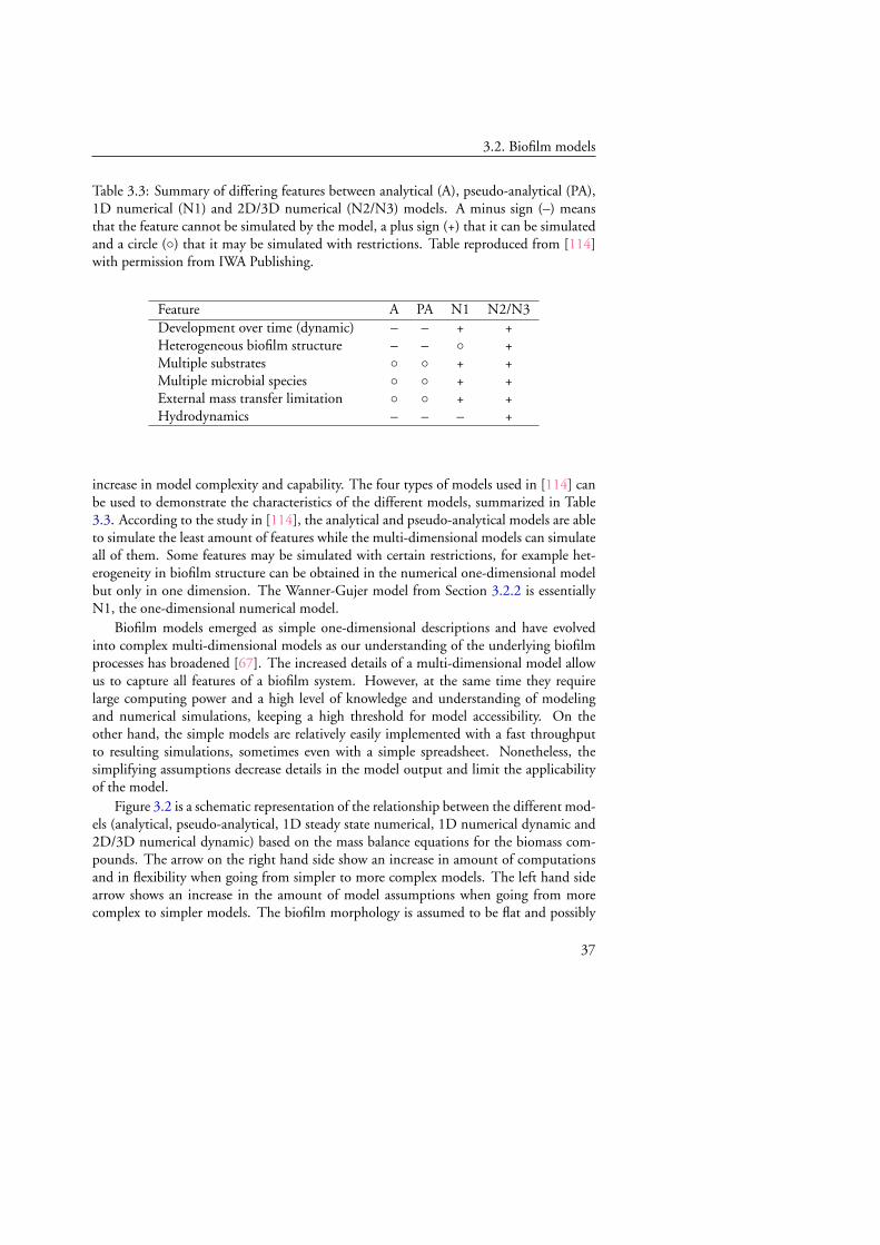
3.2. Biofilm models
Table 3.3: Summary of differing features between analytical (A), pseudo-analytical (PA),1D numerical (N1) and 2D/3D numerical (N2/N3) models. A minus sign (–) meansthat the feature cannot be simulated by the model, a plus sign (+) that it can be simulatedand a circle (◦) that it may be simulated with restrictions. Table reproduced from [114]with permission from IWA Publishing.
Feature A PA N1 N2/N3Development over time (dynamic) – – + +Heterogeneous biofilm structure – – ◦ +Multiple substrates ◦ ◦ + +Multiple microbial species ◦ ◦ + +External mass transfer limitation ◦ ◦ + +Hydrodynamics – – – +
increase in model complexity and capability. The four types of models used in [114] canbe used to demonstrate the characteristics of the different models, summarized in Table3.3. According to the study in [114], the analytical and pseudo-analytical models are ableto simulate the least amount of features while the multi-dimensional models can simulateall of them. Some features may be simulated with certain restrictions, for example het-erogeneity in biofilm structure can be obtained in the numerical one-dimensional modelbut only in one dimension. The Wanner-Gujer model from Section 3.2.2 is essentiallyN1, the one-dimensional numerical model.
Biofilm models emerged as simple one-dimensional descriptions and have evolvedinto complex multi-dimensional models as our understanding of the underlying biofilmprocesses has broadened [67]. The increased details of a multi-dimensional model allowus to capture all features of a biofilm system. However, at the same time they requirelarge computing power and a high level of knowledge and understanding of modelingand numerical simulations, keeping a high threshold for model accessibility. On theother hand, the simple models are relatively easily implemented with a fast throughputto resulting simulations, sometimes even with a simple spreadsheet. Nonetheless, thesimplifying assumptions decrease details in the model output and limit the applicabilityof the model.
Figure 3.2 is a schematic representation of the relationship between the different mod-els (analytical, pseudo-analytical, 1D steady state numerical, 1D numerical dynamic and2D/3D numerical dynamic) based on the mass balance equations for the biomass com-pounds. The arrow on the right hand side show an increase in amount of computationsand in flexibility when going from simpler to more complex models. The left hand sidearrow shows an increase in the amount of model assumptions when going from morecomplex to simpler models. The biofilm morphology is assumed to be flat and possibly
37

CHAPTER 3. Biofilm modeling
stratified in the models at the bottom of the figure. The 1D numerical dynamic modelin the middle also assume a flat biofilm surface but allow development of biofilm thick-ness and a heterogeneous microbial distribution within the biofilm. Multi-dimensionalmodels at the top of the figure include a heterogeneous biofilm surface.
Comparative studies of one- and multi-dimensional biofilm models have been per-formed in [67, 114, 123] with three benchmark problems (BM1-3) in [114]. In caseswith heterogeneous biofilm structure the various models displayed significantly differ-ent results. A two-dimensional model was able to describe the heterogeneous structurewhich led to decreases in biofilm activity and an occurrence of sloughing events [123];the one-dimensional models were unable to reproduce these local results. If global re-sults are desired, such as reactor performance, both one- and multi-dimensional modelsproduced largely the same results. Multi-species biofilms could also be represented byboth types of models, particularly with respect to substrate concentrations and fluxes.However, microbial distributions varied considerably between the models. When thecompared numerical simulations were calculated using a description of a flat biofilm theresults were not significantly different. For a relatively smooth biofilm morphology therewas a good agreement between the models. The difference was instead noticed in theefforts involved in producing the results [67]. Multi-dimensional models have higher re-quirements on input data, modifications of custom made software and ample computingresources. Numerical one-dimensional models were easily and quickly solved with avail-able software packages. Hence, simple models like the analytical, pseudo-analytical or 1Dnumerical models provide a good results-to-effort-ratio and are often recommended forusage, specifically for practitioners.
From the viewpoint of the Wanner-Gujer model, additional assumptions can bemade, which leads to more simplified models [93]. These models are often not dynami-cal and may use several approximations, but are easier to work with. On the other hand,by relaxing the assumptions more complex models are obtained [1, 28, 56, 85, 124].Different modeling approaches are used, such as individual-based modeling, cellularautomata and continuum models. Multi-dimensional, multi-species/-substrate modelsinclude many more details, but are exclusively numerical and require large computingpower. Although multi-dimensional, complex models are much better at describing localbiofilm development, they are unsuitable for large scale applications. In particular, thesemodels are not aimed at reactor scale development in the context of wastewater engineer-ing. The overall reactor system length and time scales are so much larger than the scales ofdetailed biofilm growth. The sophisticated, complex models are already computationallyheavy and are, therefore, in practice not feasible for large scale purposes. Most often, themain interest of reactor models is the longterm behavior, in which case detailed biofilmdescription is not crucial and simpler biofilm models may be used instead.
Another advantage of simple models is their suitability for mathematical analysis.Biofilm models are often collections of several types of diffusion/reaction/transport equa-tions and multi-dimensional models complicate things further. Available mathematical
38
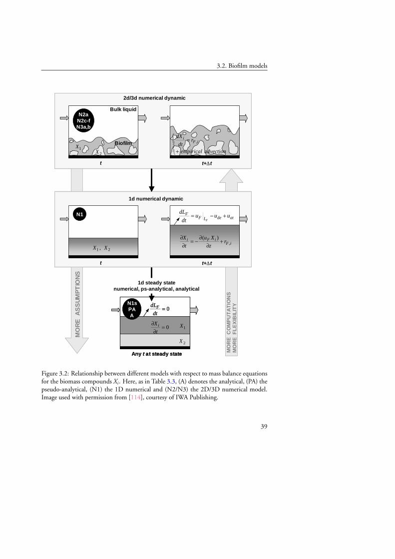
3.2. Biofilm models
Biofilm models 73
Bulk liquid
Biofilm
2d/3d numerical dynamic
t t+Δt
1d numerical dynamic
t t+Δt
Any t at steady state
1d steady state numerical, ps-analytical, analytical
,( )i F i
F iX u X
rt z
∂ ∂= − +
∂ ∂
F
FF de atL
dLu u u
dt= − +
0FdL
dt=
0iX
t
∂=
∂1X
2X
1 2,X X
1X2X
,i
F idX
rdtempirical advection
⎧ =⎪⎨⎪+⎩
MO
RE
AS
SU
MP
TIO
NS
MO
RE
CO
MP
UT
AT
ION
SM
OR
E F
LE
XIB
ILIT
Y
N2aN2c-fN3a,b
N1
N1sPAA
(b)
Figure 3.3. Schematic relationship among various models used in this report, based on derivation of mass balance equations for: (a) Soluble components; (b) Particulate (biomass) components.
Figure 3.2: Relationship between different models with respect to mass balance equationsfor the biomass compounds Xi. Here, as in Table 3.3, (A) denotes the analytical, (PA) thepseudo-analytical, (N1) the 1D numerical and (N2/N3) the 2D/3D numerical model.Image used with permission from [114], courtesy of IWA Publishing.
39

CHAPTER 3. Biofilm modeling
tools can be applied to simple or even further simplified models, depending on the spe-cific situation. Often, however, even very simple models are complex enough for reachinga limit with what is possible in mathematical analysis. There exist a few studies in whichbiofilms have been analyzed with mathematical tools. Steady state solutions of a singlespecies single substrate biofilm model with a constant bulk substrate concentration wereinvestigated in [88]. Detachment effects were not included in the model. It was shownthat the existence and stability of steady state solutions depend on biomass decay rate,maximum growth rate and bulk substrate concentration. In [107] detachment was in-cluded and global existence and properties of solutions were shown. The steady state casewas studied and existence and uniqueness of solutions were proven along with establish-ment of sufficient conditions for existence. The Freter model, describing the interactionbetween suspended and wall-attached bacteria, was analyzed in [49] where it was foundthat the trivial equilibrium (i.e. complete washout of all biomass) always exists. The sta-bility thereof depends on the growth and decay rates of the wall-attached and suspendedbiomass along with the dilution rate in the continuous-flow reactor. Moreover, it wasshown that a non-trivial equilibrium exists, but the model complexity prevented furtheranalysis.
The contribution of this thesis is to develop and study a mathematical model of abiofilm reactor with suspended growth. The main application of the models used in thisthesis is a (at times idealized) reactor in wastewater treatment. To this end, a simple,one-dimensional biofilm model has been used to describe the biofilm contribution to thereactor performance. Particular attention has been given to suspended biomass, which ismostly neglected in biofilm models.
Even though the term "simple" typically indicates a lack of complexity, the under-lying mathematical expressions are indeed rather complicated. The model presented inPaper I, with growth of biofilm and suspended biomass in a CSTR, is a hybrid modelconsisting of chemostat-like mass balances for the substrate and biomass in the reactor,coupled with a free boundary value problem for the substrate in the biofilm. The modelcould formally be rewritten as a system of ordinary differential equations to which stan-dard analytical techniques could be applied. It was shown that the stability conditionsfor the trivial equilibrium depend on the dilution rate and on the growth and decay ratesof the biofilm and the suspended biomass. In comparison with the less complex Fretermodel it was found that the main existence and stability results carry over. In the caseof an unstable washout equilibrium the system attains a non-trivial steady state at whichbiomass will exist in both forms. Numerical simulations showed that biofilm dominatesover suspended biomass in longterm reactor behavior, but that suspended biomass is rel-atively more efficient at substrate consumption.
The results from the analytical and numerical analyses in Paper I raise two follow-upquestions: (i) What happens if the substrate and treatment time are limited? (ii) What ifthe model is more biologically complex, to better represent a nitrification reactor? Thefirst question leads to an optimal control problem in Paper IV in which a biological treat-
40
3.2. Biofilm models
ment reactor is available for a limited amount of substrate stored in a buffer tank duringa limited amount of time. The aim of the optimal control problem is to increase sub-strate removal efficiency and reduce process duration while controlling the flow betweenthe buffer tank and the treatment reactor. A single species single substrate system is usedin which biofilm and suspended biomass are present. The second question leads to anextension of the model in Paper III, where a multi-substrate multi-species nitrificationmodel is presented. Ammonium oxidizing bacteria convert ammonium to nitrite, whichis in turn converted to nitrate by nitrite oxidizing bacteria. The continuous-flow stirredtank reactor is constantly oxygenated in order to supply oxygen to the aerobic reactions.The extended model requires a larger amount of parameters, why an experimental andnumerical study was performed in Paper II to validate the choice of parameters. Theunderlying model is a hybrid model consisting of a chemostat-like ordinary differentialequation model for the substrates and the suspended biomass in the reactor, coupled witha mixed hyperbolic-parabolic free boundary value problem for the biofilm. Numericalsimulations of the extended model served as a basis for the analysis.
41

CHAPTER 3. Biofilm modeling
42

Chapter 4
Conclusions and outlook
The main objective of the work presented in this thesis was to investigate the role ofsuspended biomass in biofilm reactor models. Traditional biofilm models neglect thecontribution of suspended biomass to substrate conversion. On the other hand, in modelsof the IFAS process it needs to be included as a full activated sludge model. The modelformulated in this thesis falls between these two extremes.
The model presented in Paper I is a one-dimensional biofilm reactor model of Wanner-Gujer type, based on the Freter model for wall attached bacterial growth, with a naturalexchange of biomass through attachment and detachment between the biofilm and thesuspended biomass. In a simple single species single substrate setting, but with a properdiffusion-reaction equation for the substrate in the biofilm, the model was already morecomplex than the Freter model. The analysis in Paper I showed, however, that the quali-tative results for the Freter model largely carry over. Bacteria will either be washed out orcoexist as biofilms and suspended biomass. Furthermore, numerical simulations showedthat suspended biomass was relatively more efficient at substrate removal than biofilms,even if the main contribution to removal came from the biofilm. It was found in studiesof longterm behavior that the amount of suspended biomass, relative to biofilm, dependson the dilution rate. A computational study of an extended model for the considerablymore complex multi-species multi-substrate nitrification setting in Paper III revealed thatthe incorporation of suspended biomass is significant for detailed descriptions of the pro-cesses and products in the intermediate steps of nitrification. Nevertheless, suspendedbiomass did not affect the overall reactor performance results and probably need not beconsidered if such results are the sole objective. Preparation and validation of the nitri-fication biofilm model (without suspended biomass) by comparison with microelectrodemeasurements of oxygen profiles across the biofilm was performed in Paper II. A corre-spondence between the bulk flow velocity and the thickness of the biofilm and of the masstransfer boundary layer was shown in that study, along with a dependence of the erosion
43

CHAPTER 4. Conclusions and outlook
parameter on the bulk flow velocity. The amount of wastewater to be treated is not always"infinite" and some situations require only a certain amount of wastewater to be treatedin finite time. The optimization problem presented in Paper IV addressed this situation,where the control was the flow regime between a storage tank holding the water to betreated and a treatment reactor. It was found in that study that the potential for reactorimprovement by varying the system flow rate is relatively modest. The improvement isprimarily due to an initial transient phase during which the bacteria in the reactor adjustto the environmental conditions. Since the initial conditions in the reactor are usuallynot known, the implementation of such a control is also impractical.
Simple mathematical models are considered to be a valuable tool in biofilm processresearch. They provide the opportunity for quantitative and/or qualitative analysis whileremaining informative on the overall reactor performance level. The mathematical anal-ysis builds a foundation and a framework within which further modifications and devel-opments can be made. The models presented in this thesis emphasize the significance ofsuspended biomass in biofilm models. Its effects are generally not visible on a large-scalereactor level, but may be important on a more detailed level such as the intermediatesteps in a nitrification reactor. The non-trivial equilibrium is attained when the washoutequilibrium is unstable and the two biomass forms will coexist (at some ratio). Manyinteresting applications may be (re-)evaluated with suspended biomass in mind.
The modeling community would benefit from further analytical progress in biofilmmodeling and more attention should be given to that. Mathematical tools can be usedto solidify existing or derive new models, but perhaps mostly to analyze and explain theirbehavior. There is much to learn from mathematical analysis, which is, however, rarely astraightforward task, even for relatively simple models.
The two core issues in biofilm models with suspended growth are the interactionbetween the biofilm and the suspended biomass, and the characterization of suspendedbiomass. Interaction is described by attachment and detachment processes, in this thesisexpressed as simple functions of the suspended biomass density and biofilm thickness.These processes are poorly understood in general and in biofilm reactors in particular.Many researchers use certain expressions out of convenience, but it would be helpfulto have guidelines, which expressions work best for different types of reactors. In thisthesis, suspended biomass has in essence been described as detached biofilms, even byusing the same parameters as for biofilms in the numerical simulations. There is a lackof experimental work that deals with suspended biomass in biofilm reactors. Such workwould be crucial for mathematical modeling and for understanding the role of suspendedbiomass in biofilm reactors. Regardless of the possible conclusions, there would be manythings to learn along the way.
In Paper II, the reactor flow rate was quantitatively correlated with the biomass ero-sion coefficient and the mass transfer boundary layer thickness. It would be important toinvestigate whether such results can be found for other reactor types, and if so, whetherthere is a resemblance of correlations across various reactor types.
44
A natural extension of the current work would be to consider a plug flow or horizontalflow biofilm reactor instead of a CSTR. For single species models some work has beendone in the context of the Freter model, but not considering a biofilm model to describewall attached bacteria. Such a setup could also allow for a mathematical investigationinto the role of bacterial cell yield and biofilm dispersal as a method for downstreamcolonization and biofilm proliferation. Mathematically, this would require an extensionto partial differential equations and therefore induce an additional level of complexity.
Although the optimization study presented in Paper IV led to the conclusion that thecontrolled reactor was only modestly better than the uncontrolled reactor, the approachwith optimal control problems might still be interesting for biofilm models, probably inthe context of other reactor types. Solving an optimal control problem can assist theprogress of understanding the principal features of the model. There is more to be donein regard to the optimization problem in Paper IV, where a more general solution couldbe sought both analytically and numerically. The relatively simple model is still verycomplex, using some non-standard expressions, which makes it difficult to solve. Lookinginto methods from the field of automatic control could perhaps be fruitful. Moreover,it would be interesting to investigate the optimal control problem for the multi-speciesmulti-substrate model from Paper III and compare with the results obtained in PaperIV. Would the added microbial complexity lead to qualitatively different or perhaps verysimilar results, in particular with respect to the off-on functions? Process optimization isnot unusual in wastewater engineering and an optimal control study of biofilm reactormodels would perhaps bring some new features to light. In addition, control problemsfor other types of biofilm reactors could be studied.
45

CHAPTER 4. Conclusions and outlook
46

Bibliography
[1] E. Alpkvist and I. Klapper. A multidimensional multispecies continuum modelfor heterogeneous biofilm development. Bull. Math. Biol., 69(2):765–789, 2007.
[2] R.I. Amann, W. Ludwig, and K.H. Schleifer. Phylogenetic identification and insitu detection of individual microbial cells without cultivation. Microbiol. Mol.Biol. Rev., 59(1):143–169, 1995.
[3] M.M. Ballyk, D.A. Jones, and H.L. Smith. Microbial competition in reactors withwall attachment: A mathematical comparison of chemostat and plug flow models.Microb. Ecol., 41(3):210–221, 2001.
[4] M.M. Ballyk, D.A. Jones, and H.L. Smith. The biofilm model of Freter: A review.In P. Magal and S. Ruan, editors, Structured population models in biology and epi-demiology, volume 1936 of Springer lecture notes in mathematics, pages 265–302.Springer, Berlin, 2008.
[5] J.P. Boltz, D. Brockmann, T. Sandy, B.R. Johnson, G.T. Daigger, K. Jenkins, andK. Munirathinam. Framework for a mixed-culture biofilm model to describe ox-idized nitrogen, sulfur, and selenium removal in a biofilm reactor. In Proceedingsof the Water Environment Federation, WEFTEC 2011: Session 1 through Session 10,pages 145–156, 2011.
[6] J.P. Boltz, B.R. Johnson, G.T. Daigger, and J. Sandino. Modeling integrated fixed-film activated sludge and moving-bed biofilm reactor systems I: Mathematicaltreatment and model development. Water Environ. Res., 81(6):555–575, 2009.
[7] J.P. Boltz, E. Morgenroth, D. Brockmann, C. Bott, W.J. Gellner, and P.A. Vanrol-leghem. Critical components of biofilm models for engineering practice. In Pro-ceedings of the Water Environment Federation, WEFTEC 2010: Session 21 throughSession 30, pages 1072–1098, 2010.
47

BIBLIOGRAPHY
[8] J.P. Boltz, E. Morgenroth, and D. Sen. Mathematical modelling of biofilms andbiofilm reactors for engineering design. Water Sci. Technol., 62(8):1821–1836,2010.
[9] M.G. Brading, J. Jass, and H.M. Lappin-Scott. Dynamics of bacterial biofilmformation. In H.M. Lappin-Scott and J.W. Costerton, editors, Microbial biofilms,pages 46–63. Cambridge University Press, Cambridge, United Kingdom, 1995.
[10] D. Brockmann, K.-H. Rosenwinkel, and E. Morgenroth. Practical identifiabilityof biokinetic parameters of a model describing two-step nitrification in biofilms.Biotechnol. Bioeng., 101(3):497–514, 2008.
[11] J.D. Bryers. Biofilms and the technological implications of microbial cell adhesion.Colloids Surf., B, 2(1-3):9–23, 1994.
[12] A. Cébron and J. Garnier. Nitrobacter and Nitrospira genera as representatives ofnitrite-oxidizing bacteria: Detection, quantification and growth along the lowerSeine River (France). Water Res., 39(20):4979–4992, 2005.
[13] S. Chen, J. Ling, and J.-P. Blancheton. Nitrification kinetics of biofilm as affectedby water quality factors. Aquacult. Eng., 34(3):179–197, 2006.
[14] N. Cogan, B. Szomolay, and M. Dindos. Effect of periodic disinfection on persis-ters in a one-dimensional biofilm model. Bull. Math. Biol., 75(1):94–123, 2013.
[15] D.L. Correll. The role of phosphorus in the eutrophication of receiving waters: Areview. J. Environ. Qual., 27(2):261–266, 1998.
[16] J.W. Costerton. Overview of microbial biofilms. J. Ind. Microbiol., 15(3):137–140, 1995.
[17] J.W. Costerton and H.M. Lappin-Scott. Introduction to microbial biofilms. InH.M. Lappin-Scott and J.W. Costerton, editors, Microbial biofilms, pages 1–11.Cambridge University Press, Cambridge, United Kingdom, 1995.
[18] J.W. Costerton, Z. Lewandowski, D.E. Caldwell, D.R. Korber, and H.M. Lappin-Scott. Microbial biofilms. Annu. Rev. Microbiol., 49:711–745, 1995.
[19] J.W. Costerton, P.S. Stewart, and E.P. Greenberg. Bacterial biofilms: a commoncause of persistent infections. Science, 284(5418):1318–1322, 1999.
[20] M.E. Davey and G.A. O’Toole. Microbial biofilms: from ecology to moleculargenetics. Microbiol. Mol. Biol. Rev., 64(4):847–867, 2000.
[21] D.G. Davies. Biofilm dispersion. In H.-C. Flemming, J. Wingender, andU. Szewzyk, editors, Biofilm highlights, volume 5 of Springer series on biofilms, pages1–28. Springer, Berlin, 2011.
48

BIBLIOGRAPHY
[22] D. de Beer and A. Schramm. Micro-environments and mass transfer phenomenain biofilms studied with microsensors. Water Sci. Technol., 39(7):173–178, 1999.
[23] D. de Beer, P. Stoodley, F. Roe, and Z. Lewandowski. Effects of biofilm structureson oxygen distribution and mass transport. Biotechnol. Bioeng., 43(11):1131–1138, 1994.
[24] W.M. Deen. Analysis of transport phenomena. Topics in Chemical Engineering.Oxford University Press, USA, 1998.
[25] R.M. Donlan. Biofilm formation: a clinically relevant microbiological process.Clin. Infect. Dis., 33(8):1387–1392, 2001.
[26] R.M. Donlan. Biofilms: microbial life on surfaces. Emerg. Infect. Dis., 8(9):881–890, 2002.
[27] W.M. Dunne. Bacterial adhesion: Seen any good biofilms lately? Clin. Microbiol.Rev., 15(2):155–166, 2002.
[28] H.J. Eberl, D.F. Parker, and M.C.M. van Loosdrecht. A new deterministic spatio-temporal continuum model for biofilm development. J. Theor. Med., 3(3):161–175, 2001.
[29] L. Edelstein-Keshet. Mathematical models in biology. Classics in Applied Mathe-matics. Society for Industrial and Applied Mathematics, Philadelphia, USA, 2005.
[30] C.M. Falkentoft, P. Arnz, M. Henze, H. Mosbæk, E. Müller, P.A. Wilderer, andP. Harremoës. Possible complication regarding phosphorus removal with a contin-uous flow biofilm system: Diffusion limitation. Biotechnol. Bioeng., 76(1):77–85,2001.
[31] H. Fgaier and H.J. Eberl. A competition model between Pseudomonas fluorescensand pathogens via iron chelation. J. Theor. Biol., 263(4):566–578, 2010.
[32] H.-C. Flemming. Biofouling in water systems - cases, causes and countermeasures.Appl. Microbiol. Biotechnol., 59(6):629–640, 2002.
[33] H.-C. Flemming, T.R. Neu, and D.J. Wozniak. The EPS matrix: The "house ofbiofilm cells". J. Bacteriol., 189(22):7945–7947, 2007.
[34] R. Freter, H. Brickner, J. Fekete, M. Vickerman, and K. Carey. Survival andimplantation of Escherichia coli in the intestinal tract. Infect. Immun., 39(2):686–703, 1983.
[35] H. Furumai and B.E. Rittmann. Evaluation of multiple-species biofilm and flocprocesses using a simplified aggregate model. Water Sci. Technol., 29(10-11):439–446, 1994.
49
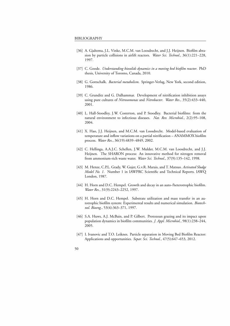
BIBLIOGRAPHY
[36] A. Gjaltema, J.L. Vinke, M.C.M. van Loosdrecht, and J.J. Heijnen. Biofilm abra-sion by particle collisions in airlift reactors. Water Sci. Technol., 36(1):221–228,1997.
[37] C. Goode. Understanding biosolids dynamics in a moving bed biofilm reactor. PhDthesis, University of Toronto, Canada, 2010.
[38] G. Gottschalk. Bacterial metabolism. Springer-Verlag, New York, second edition,1986.
[39] C. Grunditz and G. Dalhammar. Development of nitrification inhibition assaysusing pure cultures of Nitrosomonas and Nitrobacter. Water Res., 35(2):433–440,2001.
[40] L. Hall-Stoodley, J.W. Costerton, and P. Stoodley. Bacterial biofilms: from thenatural environment to infectious diseases. Nat. Rev. Microbiol., 2(2):95–108,2004.
[41] X. Hao, J.J. Heijnen, and M.C.M. van Loosdrecht. Model-based evaluation oftemperature and inflow variations on a partial nitrification – ANAMMOX biofilmprocess. Water Res., 36(19):4839–4849, 2002.
[42] C. Hellinga, A.A.J.C. Schellen, J.W. Mulder, M.C.M. van Loosdrecht, and J.J.Heijnen. The SHARON process: An innovative method for nitrogen removalfrom ammonium-rich waste water. Water Sci. Technol., 37(9):135–142, 1998.
[43] M. Henze, C.P.L. Grady, W. Gujer, G.v.R. Marais, and T. Matsuo. Activated SludgeModel No. 1. Number 1 in IAWPRC Scientific and Technical Reports. IAWQLondon, 1987.
[44] H. Horn and D.C. Hempel. Growth and decay in an auto-/heterotrophic biofilm.Water Res., 31(9):2243–2252, 1997.
[45] H. Horn and D.C. Hempel. Substrate utilization and mass transfer in an au-totrophic biofilm system: Experimental results and numerical simulation. Biotech-nol. Bioeng., 53(4):363–371, 1997.
[46] S.A. Huws, A.J. McBain, and P. Gilbert. Protozoan grazing and its impact uponpopulation dynamics in biofilm communities. J. Appl. Microbiol., 98(1):238–244,2005.
[47] I. Ivanovic and T.O. Leiknes. Particle separation in Moving Bed Biofilm Reactor:Applications and opportunities. Separ. Sci. Technol., 47(5):647–653, 2012.
50
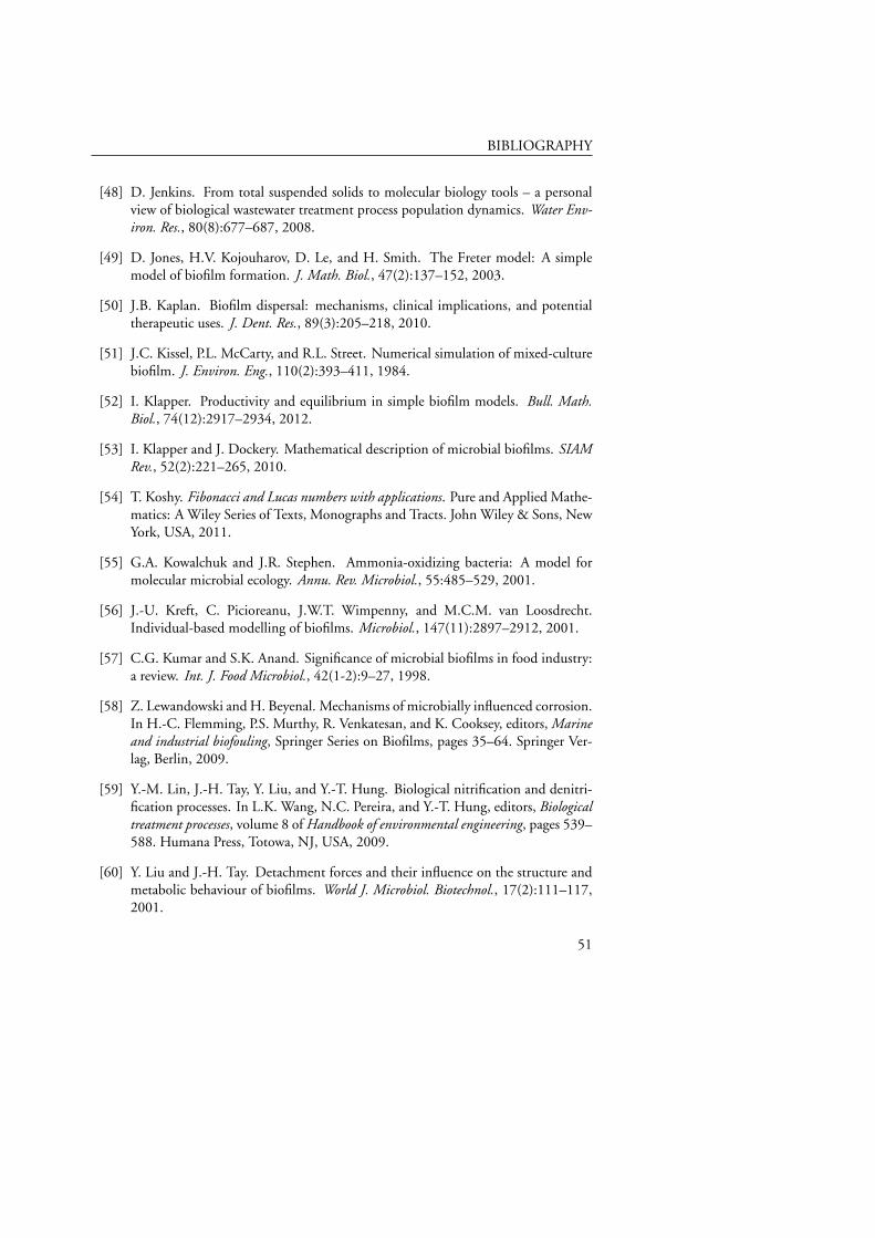
BIBLIOGRAPHY
[48] D. Jenkins. From total suspended solids to molecular biology tools – a personalview of biological wastewater treatment process population dynamics. Water Env-iron. Res., 80(8):677–687, 2008.
[49] D. Jones, H.V. Kojouharov, D. Le, and H. Smith. The Freter model: A simplemodel of biofilm formation. J. Math. Biol., 47(2):137–152, 2003.
[50] J.B. Kaplan. Biofilm dispersal: mechanisms, clinical implications, and potentialtherapeutic uses. J. Dent. Res., 89(3):205–218, 2010.
[51] J.C. Kissel, P.L. McCarty, and R.L. Street. Numerical simulation of mixed-culturebiofilm. J. Environ. Eng., 110(2):393–411, 1984.
[52] I. Klapper. Productivity and equilibrium in simple biofilm models. Bull. Math.Biol., 74(12):2917–2934, 2012.
[53] I. Klapper and J. Dockery. Mathematical description of microbial biofilms. SIAMRev., 52(2):221–265, 2010.
[54] T. Koshy. Fibonacci and Lucas numbers with applications. Pure and Applied Mathe-matics: A Wiley Series of Texts, Monographs and Tracts. John Wiley & Sons, NewYork, USA, 2011.
[55] G.A. Kowalchuk and J.R. Stephen. Ammonia-oxidizing bacteria: A model formolecular microbial ecology. Annu. Rev. Microbiol., 55:485–529, 2001.
[56] J.-U. Kreft, C. Picioreanu, J.W.T. Wimpenny, and M.C.M. van Loosdrecht.Individual-based modelling of biofilms. Microbiol., 147(11):2897–2912, 2001.
[57] C.G. Kumar and S.K. Anand. Significance of microbial biofilms in food industry:a review. Int. J. Food Microbiol., 42(1-2):9–27, 1998.
[58] Z. Lewandowski and H. Beyenal. Mechanisms of microbially influenced corrosion.In H.-C. Flemming, P.S. Murthy, R. Venkatesan, and K. Cooksey, editors, Marineand industrial biofouling, Springer Series on Biofilms, pages 35–64. Springer Ver-lag, Berlin, 2009.
[59] Y.-M. Lin, J.-H. Tay, Y. Liu, and Y.-T. Hung. Biological nitrification and denitri-fication processes. In L.K. Wang, N.C. Pereira, and Y.-T. Hung, editors, Biologicaltreatment processes, volume 8 of Handbook of environmental engineering, pages 539–588. Humana Press, Totowa, NJ, USA, 2009.
[60] Y. Liu and J.-H. Tay. Detachment forces and their influence on the structure andmetabolic behaviour of biofilms. World J. Microbiol. Biotechnol., 17(2):111–117,2001.
51
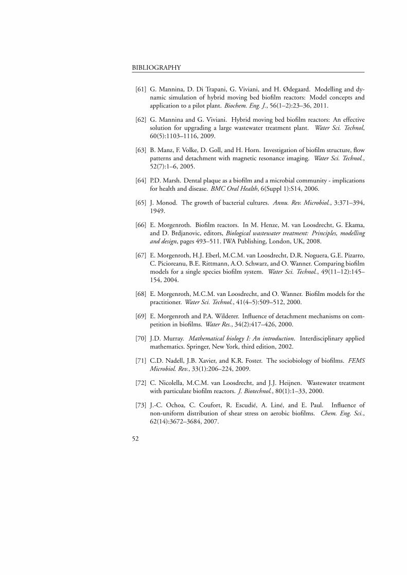
BIBLIOGRAPHY
[61] G. Mannina, D. Di Trapani, G. Viviani, and H. Ødegaard. Modelling and dy-namic simulation of hybrid moving bed biofilm reactors: Model concepts andapplication to a pilot plant. Biochem. Eng. J., 56(1–2):23–36, 2011.
[62] G. Mannina and G. Viviani. Hybrid moving bed biofilm reactors: An effectivesolution for upgrading a large wastewater treatment plant. Water Sci. Technol,60(5):1103–1116, 2009.
[63] B. Manz, F. Volke, D. Goll, and H. Horn. Investigation of biofilm structure, flowpatterns and detachment with magnetic resonance imaging. Water Sci. Technol.,52(7):1–6, 2005.
[64] P.D. Marsh. Dental plaque as a biofilm and a microbial community - implicationsfor health and disease. BMC Oral Health, 6(Suppl 1):S14, 2006.
[65] J. Monod. The growth of bacterial cultures. Annu. Rev. Microbiol., 3:371–394,1949.
[66] E. Morgenroth. Biofilm reactors. In M. Henze, M. van Loosdrecht, G. Ekama,and D. Brdjanovic, editors, Biological wastewater treatment: Principles, modellingand design, pages 493–511. IWA Publishing, London, UK, 2008.
[67] E. Morgenroth, H.J. Eberl, M.C.M. van Loosdrecht, D.R. Noguera, G.E. Pizarro,C. Picioreanu, B.E. Rittmann, A.O. Schwarz, and O. Wanner. Comparing biofilmmodels for a single species biofilm system. Water Sci. Technol., 49(11–12):145–154, 2004.
[68] E. Morgenroth, M.C.M. van Loosdrecht, and O. Wanner. Biofilm models for thepractitioner. Water Sci. Technol., 41(4–5):509–512, 2000.
[69] E. Morgenroth and P.A. Wilderer. Influence of detachment mechanisms on com-petition in biofilms. Water Res., 34(2):417–426, 2000.
[70] J.D. Murray. Mathematical biology I: An introduction. Interdisciplinary appliedmathematics. Springer, New York, third edition, 2002.
[71] C.D. Nadell, J.B. Xavier, and K.R. Foster. The sociobiology of biofilms. FEMSMicrobiol. Rev., 33(1):206–224, 2009.
[72] C. Nicolella, M.C.M. van Loosdrecht, and J.J. Heijnen. Wastewater treatmentwith particulate biofilm reactors. J. Biotechnol., 80(1):1–33, 2000.
[73] J.-C. Ochoa, C. Coufort, R. Escudié, A. Liné, and E. Paul. Influence ofnon-uniform distribution of shear stress on aerobic biofilms. Chem. Eng. Sci.,62(14):3672–3684, 2007.
52
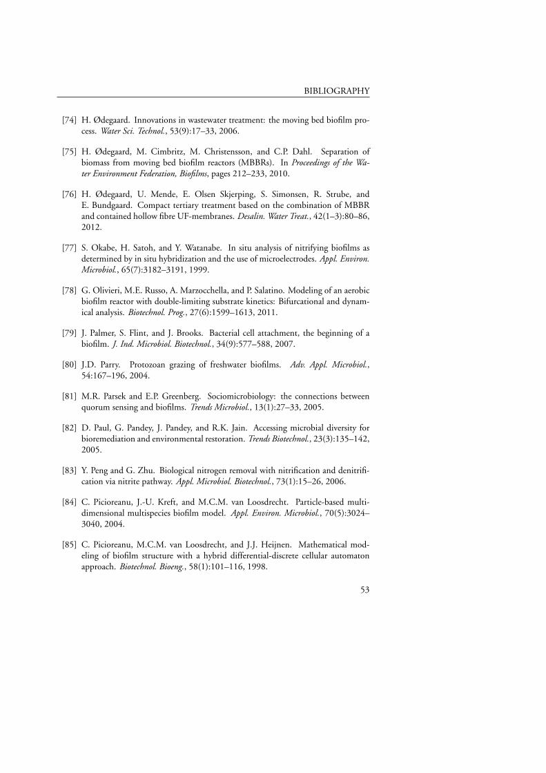
BIBLIOGRAPHY
[74] H. Ødegaard. Innovations in wastewater treatment: the moving bed biofilm pro-cess. Water Sci. Technol., 53(9):17–33, 2006.
[75] H. Ødegaard, M. Cimbritz, M. Christensson, and C.P. Dahl. Separation ofbiomass from moving bed biofilm reactors (MBBRs). In Proceedings of the Wa-ter Environment Federation, Biofilms, pages 212–233, 2010.
[76] H. Ødegaard, U. Mende, E. Olsen Skjerping, S. Simonsen, R. Strube, andE. Bundgaard. Compact tertiary treatment based on the combination of MBBRand contained hollow fibre UF-membranes. Desalin. Water Treat., 42(1–3):80–86,2012.
[77] S. Okabe, H. Satoh, and Y. Watanabe. In situ analysis of nitrifying biofilms asdetermined by in situ hybridization and the use of microelectrodes. Appl. Environ.Microbiol., 65(7):3182–3191, 1999.
[78] G. Olivieri, M.E. Russo, A. Marzocchella, and P. Salatino. Modeling of an aerobicbiofilm reactor with double-limiting substrate kinetics: Bifurcational and dynam-ical analysis. Biotechnol. Prog., 27(6):1599–1613, 2011.
[79] J. Palmer, S. Flint, and J. Brooks. Bacterial cell attachment, the beginning of abiofilm. J. Ind. Microbiol. Biotechnol., 34(9):577–588, 2007.
[80] J.D. Parry. Protozoan grazing of freshwater biofilms. Adv. Appl. Microbiol.,54:167–196, 2004.
[81] M.R. Parsek and E.P. Greenberg. Sociomicrobiology: the connections betweenquorum sensing and biofilms. Trends Microbiol., 13(1):27–33, 2005.
[82] D. Paul, G. Pandey, J. Pandey, and R.K. Jain. Accessing microbial diversity forbioremediation and environmental restoration. Trends Biotechnol., 23(3):135–142,2005.
[83] Y. Peng and G. Zhu. Biological nitrogen removal with nitrification and denitrifi-cation via nitrite pathway. Appl. Microbiol. Biotechnol., 73(1):15–26, 2006.
[84] C. Picioreanu, J.-U. Kreft, and M.C.M. van Loosdrecht. Particle-based multi-dimensional multispecies biofilm model. Appl. Environ. Microbiol., 70(5):3024–3040, 2004.
[85] C. Picioreanu, M.C.M. van Loosdrecht, and J.J. Heijnen. Mathematical mod-eling of biofilm structure with a hybrid differential-discrete cellular automatonapproach. Biotechnol. Bioeng., 58(1):101–116, 1998.
53
BIBLIOGRAPHY
[86] C. Picioreanu, M.C.M. van Loosdrecht, and J.J. Heijnen. A new combineddifferential-discrete cellular automaton approach for biofilm modeling: Applica-tion for growth in gel beads. Biotechnol. Bioeng., 57(6):718–731, 1998.
[87] C. Picioreanu, J.B. Xavier, and M.C.M. van Loosdrecht. Advances in mathemati-cal modeling of biofilm structure. Biofilms, 1(4):337–349, 2004.
[88] L.A. Pritchett and J.D. Dockery. Steady state solutions of a one-dimensionalbiofilm model. Math. Comput. Model., 33(1–3):255–263, 2001.
[89] C.W. Randall and D. Sen. Full-scale evaluation of an integrated fixed-film acti-vated sludge (IFAS) process for enhanced nitrogen removal. Water Sci. Technol.,33(12):155–162, 1996.
[90] P. Reichert. AQUASIM - A tool for simulation and data analysis of aquatic systems.Water Sci. Technol., 30(2):21–30, 1994.
[91] R. Riffat. Fundamentals of wastewater treatment and engineering. CRC Press / IWAPublishing, 2012.
[92] B.E. Rittmann. The effect of shear stress on biofilm loss rate. Biotechnol. Bioeng.,24(2):501–506, 1982.
[93] B.E. Rittmann and P.L. McCarty. Model of steady-state-biofilm kinetics. Biotech-nol. Bioeng., 22(11):2343–2357, 1980.
[94] M.E. Roberts and P.S. Stewart. Modeling antibiotic tolerance in biofilms by ac-counting for nutrient limitation. Antimicrob. Agents Chemother., 48(1):48–52,2004.
[95] M. Rodgers and X.-M. Zhan. Moving-medium biofilm reactors. Rev. Environ. Sci.Biotechnol., 2(2-4):213–224, 2003.
[96] B. Rosche, X.Z. Li, B. Hauer, A. Schmid, and K. Buehler. Microbial biofilms: aconcept for industrial catalysis? Trends Biotechnol., 27(11):636–643, 2009.
[97] M.E. Russo, P.L. Maffettone, A. Marzocchella, and P. Salatino. Bifurcational anddynamical analysis of a continuous biofilm reactor. J. Biotechnol., 135(3):295–303,2008.
[98] K. Sauer, M.C. Cullen, A.H. Rickard, L.A.H. Zeef, D.G. Davies, and P. Gilbert.Characterization of nutrient-induced dispersion in Pseudomonas aeruginosa PAO1biofilm. J. Bacteriol., 186(21):7312–7326, 2004.
[99] R.P. Schneider. Conditioning film-induced modification of substratum physic-ochemistry – analysis by contact angles. J. Colloid Interface Sci., 182:204–213,1996.
54
BIBLIOGRAPHY
[100] A. Schramm, L.H. Larsen, N.P. Revsbech, N.B. Ramsing, R. Amann, and K.H.Schleifer. Structure and function of a nitrifying biofilm as determined by insitu hybridization and the use of microelectrodes. Appl. Environ. Microbiol.,62(12):4641–4647, 1996.
[101] B. Sharma and R.C. Ahlert. Nitrification and nitrogen removal (in waste watertreatment). Water Res., 11(10):897–925, 1977.
[102] H.L. Smith and P. Waltman. The theory of the chemostat: Dynamics of microbialcompetition. Cambridge University Press, Cambridge, UK, 1995.
[103] E.D. Stemmons and H.L. Smith. Competition in a chemostat with wall attach-ment. SIAM J. Appl. Math., 61(2):567–595, 2000.
[104] P.S. Stewart. Diffusion in biofilms. J. Bacteriol., 185(5):1485–1491, 2003.
[105] P.S. Stewart and M.J. Franklin. Physiological heterogeneity in biofilms. Nat. Rev.Microbiol., 6(3):199–210, 2008.
[106] P. Stoodley, K. Sauer, D.G. Davies, and J.W. Costerton. Biofilms as complexdifferentiated communities. Annu. Rev. Microbiol., 56:187–209, 2002.
[107] B. Szomolay. Analysis of a moving boundary value problem arising in biofilmmodelling. Math. Methods Appl. Sci., 31(15):1835–1859, 2008.
[108] B. Szomolay, I. Klapper, and M. Dindos. Analysis of adaptive response to dosingprotocols for biofilm control. SIAM J. Appl. Math., 70(8):3175–3202, 2010.
[109] U. Telgmann, H. Horn, and E. Morgenroth. Influence of growth history onsloughing and erosion from biofilms. Water Res., 38(17):3671–3684, 2004.
[110] T. Tolker-Nielsen, U.C. Brinch, P.C. Ragas, J.B. Andersen, C.S. Jacobsen, andS. Molin. Development and dynamics of Pseudomonas sp. biofilms. J. Bacteriol.,182(22):6482–6489, 2000.
[111] M. von Sperling. Activated sludge and aerobic biofilm reactors, volume 5 of Biologicalwastewater treatment series. IWA Publishing, London, UK, 2007.
[112] M. Wagner, B. Manz, F. Volke, T.R. Neu, and H. Horn. Online assessment ofbiofilm development, sloughing and forced detachment in tube reactor by meansof magnetic resonance microscopy. Biotechnol. Bioeng., 107(1):172–181, 2010.
[113] Q. Wang and T. Zhang. Review of mathematical models for biofilms. Solid StateCommun., 150(21–22):1009–1022, 2010.
55

BIBLIOGRAPHY
[114] O. Wanner, H. Eberl, E. Morgenroth, D.R. Noguera, C. Picioreanu, B. Rittmann,and M. van Loosdrecht. Mathematical modeling of biofilms. Number 18 in Scien-tific and Technical Report. IWA Publishing, London, UK, 2006.
[115] O. Wanner and W. Gujer. Competition in biofilms. Water Sci. Technol., 17(2–3):27–44, 1984.
[116] O. Wanner and W. Gujer. A multispecies biofilm model. Biotechnol. Bioeng.,28(3):314–328, 1986.
[117] O. Wanner and P. Reichert. Mathematical modeling of mixed-culture biofilms.Biotechnol. Bioeng., 49(2):172–184, 1996.
[118] Y. Watanabe, S. Masuda, and M. Ishiguro. Simultaneous nitrification and denitri-fication in micro-aerobic biofilms. Water Sci. Technol., 26(3–4):511–522, 1992.
[119] P. Watnick and R. Kolter. Biofilm, city of microbes. J. Bacteriol., 182(10):2675–2679, 2000.
[120] M. Wichern, C. Lindenblatt, M. Lübken, and H. Horn. Experimental resultsand mathematical modelling of an autotrophic and heterotrophic biofilm in a sandfilter treating landfill leachate and municipal wastewater. Water Res., 42(14):3899–3909, 2008.
[121] J. Wimpenny, W. Manz, and U. Szewzyk. Heterogeneity in biofilms. FEMSMicrobiol. Rev., 24(5):661–671, 2000.
[122] G.M. Wong-Chong and R.C. Loehr. The kinetics of microbial nitrification. WaterRes., 9(12):1099–1106, 1975.
[123] J.B. Xavier, C. Picioreanu, and M.C.M. van Loosdrecht. A modelling study of theactivity and structure of biofilms in biological reactors. Biofilms, 1(4):377–391,2004.
[124] J.B. Xavier, C. Picioreanu, and M.C.M. van Loosdrecht. A framework for multi-dimensional modelling of activity and structure of multispecies biofilms. Environ.Microbiol., 7(8):1085–1103, 2005.
[125] T.C. Zhang and P.L. Bishop. Experimental determination of the dissolved oxygenboundary layer and mass transfer resistance near the fluid-biofilm interface. WaterSci. Technol., 30(11):47–58, 1994.
[126] S. Zhu and S. Chen. The impact of temperature on nitrification rate in fixed filmbiofilters. Aquacult. Eng., 26(4):221–237, 2002.
56

Papers


PAPER I
Published in Bulletin of Mathematical Biology 2012.


PAPER I
Persistence in a single species CSTR model with suspendedflocs and wall attached biofilms
Alma Mašica,b, Hermann J. Eberlc
a) School of Technology, Malmö University, SE-20506 Malmö, Sweden.
b) Centre for Mathematical Sciences, Lund University, Box 118, SE-22100, Lund, Sweden.
E-mail: [email protected]
c) Biophysics Interdepartmental Program and Dept. Mathematics and Statistics, University of Guelph, ON, Canada,
N1G 2W1
E-mail: [email protected]
Abstract
We consider a mathematical model for a bacterial population in a continuously stirredtank reactor (CSTR) with wall attachment. This is a modification of the Freter model,in which we model the sessile bacteria as a microbial biofilm. Our analysis indicatesthat the results of the algebraically simpler original Freter model largely carry over. In acomputational simulation study, we find that the vast majority of bacteria in the reactorwill eventually be sessile. However, we also find that suspended biomass is relatively moreefficient in removing substrate from the reactor than biofilm bacteria.
Keywords: biofilm, mathematical model, CSTR, wall attachment.MSC: 92D25
1 Introduction
Bacterial biofilms are microbial layers on immersed surfaces in aqueous systems. Bacteriaadhere to the surface, become sessile and start producing a gel-like matrix of extracellu-lar polymeric substances (EPS) in which they are themselves embedded [16]. Biofilmsare omnipresent and can be found wherever environmental conditions sustain microbialgrowth. It has been suggested that the vast majority of bacteria in natural systems live inbiofilm communities [9], and not in suspended communities, which have traditionallybeen the center of study, both in experimental microbiology and in mathematical biology.
Two primary distinctions between the biofilm and the suspended mode of growthare (i) the EPS matrix offers the cells protection against mechanical washout and (ii) ina biofilm, the bacteria experience concentration gradients of dissolved substrates, i.e. theliving conditions depend on the location of the cell within the biofilm [23, 26]. The lattercan lead to the establishment of micro-environments, such as anaerobic zones in aerobicbiofilms [8, 26].
In environmental engineering many technologies have been developed based on biofilmprocesses, in particular in wastewater treatment, but also for soil remediation and ground-
61
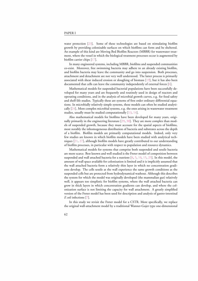
PAPER I
water protection [23]. Some of these technologies are based on stimulating biofilmgrowth by providing colonizable surfaces on which biofilms can form and be sheltered.An example of this kind are Moving Bed Biofilm Reactors (MBBR) for wastewater treat-ment, where the vessel in which the biological treatment processes occur is augmented bybiofilm carrier chips [17].
In many engineered systems, including MBBR, biofilms and suspended communitiesco-exist. Moreover, free swimming bacteria may adhere to an already existing biofilm,and biofilm bacteria may leave the community and go into suspension. Both processes,attachment and detachment are not very well understood. The latter process is primarilyassociated with shear induced erosion or sloughing of biomass [19], but it has also beendocumented that cells can leave the community independently of external forces [6].
Mathematical models for suspended bacterial populations have been successfully de-veloped for many years and are frequently and routinely used in design of reactors andoperating conditions, and in the analysis of microbial growth curves, e.g. for food safetyand shelf-life studies. Typically these are systems of first order ordinary differential equa-tions. In microbially relatively simple systems, these models can often be studied analyti-cally [24]. More complex microbial systems, e.g. the ones arising in wastewater treatmentstudies, usually must be studied computationally [13, 14].
Also mathematical models for biofilms have been developed for many years, origi-nally primarily in the engineering literature [29, 30]. They are more complex than mod-els of suspended growth, because they must account for the spatial aspects of biofilms,most notably the inhomogeneous distribution of bacteria and substrates across the depthof a biofilm. Biofilm models are primarily computational models. Indeed, only veryfew studies are known in which biofilm models have been studied with analytical tech-niques [21, 27], although biofilm models have greatly contributed to our understandingof biofilm processes, in particular with respect to population and resource dynamics.
Mathematical models for systems that comprise both suspended and sessile bacteriaare more scarce. Best known and well studied is the Freter model of competition betweensuspended and wall attached bacteria for a nutrient [4, 5, 10, 15, 25]. In this model, theamount of wall space available for colonization is limited and it is implicitly assumed thatthe wall attached bacteria form a relatively thin layer in which no concentration gradi-ents develop. The cells sessile at the wall experience the same growth conditions as thesuspended cells but are protected from hydrodynamical washout. Although this describesthe system for which the model was originally developed (the mammalian gut) relativelywell, it appears too simplistic for biofilm systems, where the wall attached bacteria cangrow in thick layers in which concentration gradients can develop, and where the col-onization surface is not limiting the capacity for wall attachment. A greatly simplifiedversion of the Freter model has been used for description and analysis of gastro-intestinalE coli infections [7].
In this study we revisit the Freter model for a CSTR. More specifically, we replacethe original wall-attachment model by a traditional Wanner-Gujer type one-dimensional
62

PAPER I
biofilm model [29, 30], in order to account for the spatial structure of the wall attachedbacterial population. The resulting model is algebraically more complex than the originalFreter model and naturally the question arises whether this added algebraic complexityalso adds new dynamic complexity. This is investigated with analytical and computa-tional methods. Moreover, in a numerical simulation experiment we investigate howreactor operating conditions, such as flow rate, bulk substrate concentration, and surfacearea available for colonization affect the reactor’s performance with respect to substrateremoval.
2 Model description
2.1 The Freter model of a CSTR with wall attachment
In [10] a model was proposed that describes the formation of a microbial populationin an aqueous environment in the mammalian gut. Bacteria can be suspended in theaqueous phase or colonize the surface. This model was later adapted to a CSTR [15],which includes the following processes:
• continuous replenishment of the reactor with fresh medium,
• washout of substrate and suspended biomass,
• growth of bacterial biomass through consumption of substrate,
• natural cell death,
• attachment of suspended biomass to the wall,
• detachment of bacteria from the wall.
This is described by a system of three ordinary differential equations for the substrateconcentration, the unattached as well as the wall-attached bacteria. The model reads
S = D(Sin − S)− γ−1(uμu(S) + δwμw(S)) (1)
u = u(μu(S)− D− ku) + βδw + δwμw(S)(1− G(W ))− αu(1−W ) (2)
w = w(μw(S)G(W )− β − kw) + αu(1−W )δ−1. (3)
The dependent variables are concentration of the growth limiting substrate S [gm−3],the concentration of suspended bacteria u [gm−3], and the amount of biomass per unitarea of colonizable surface, w [gm−2].
The parameter D [d−1] is the dilution rate, i.e. the rate at which fresh substrate issupplied to the reactor, and at which substrate and suspended bacteria are washed out.It is obtained through D = Q/V where Q [m3d−1] is the flow rate and V [m3] the
63

PAPER I
reactor volume. By Sin [gm−3] we denote the bulk concentration, i.e. the concentrationat inflow. The constant δ [m−1] is a reactor parameter that denotes how much surfacearea is available for colonization per unit volume of the reactor.
The growth rates of the unattached and wall-attached bacteria are denoted by μu(S)and μw(S), respectively. The functional relationship between growth rate and substrateconcentration is described by Monod kinetics, i.e. takes the form
μu(S) =muS
au + S, μw(S) =
mwSaw + S
,
where the constants mu [d−1] and mw [d−1] are the maximum specific growth rates, i.e.the growth rates achieved in situations of food abundance, and the parameters au [gm−3]and aw [gm−3] are the half saturation coefficients. The constant γ [−] is the biomassyield per unit of substrate. The cell death rates are ku [d−1] and kw [d−1].
Daughter cells of the wall-attached bacteria compete for space; G(W ) cells attach tothe wall at rate α [d−1], 1−G(W ) are released into the bulk liquid, where G(W ) = 1−W
1.1−Wand W := w/wmax is the wall occupancy fraction. Detachment of wall attached bacteriahappens at rate β [d−1].
It was found in [15] that the washout steady state (S, u,w) = (Sin, 0, 0) always existsand that it is locally asymptotically stable if both μw(Sin)−kw < 0 and μu(Sin)−k−D < 0are satisfied. It is unstable if either μw(Sin)G(0)− kw−β ≥ 0 or μu(Sin)− k−D−α ≥ 0is satisfied. Further, the study showed that at least one nontrivial steady state (S, u,w) =(S∗, u∗,w∗) exists when the washout state is unstable. However, given the complexity ofthe model, a calculation of the exact coordinates of the nontrivial steady state in closedform was not possible. Instability of the washout state implies persistence of u and w,assuming nontrivial initial data.
2.2 A CSTR model with wall attachment in form of biofilms
In the model of [15] the wall attached bacteria experience the same substrate concentra-tions as the suspended bacteria. We will re-formulate the model for the case where the wallattached cells form bacterial biofilms. The starting point for our model is a CSTR massbalance as in the previous section, which we couple with a traditional one-dimensionalbiofilm model. The processes included in this model are the same as in Section 2.1.Additionally, we assume that
• the biofilm uniformly covers the surface that is available for colonization,
• substrate diffuses into the bacterial biofilm layer,
• substrate gradients in the biofilm are observed as a consequence of diffusion andreaction.
64

PAPER I
In the Freter model all sessile bacteria are assumed to be wall-attached and, therefore,compete for space. On the other hand, in a biofilm, sessile bacteria grow in thick layersthat form on the substratum. In the Wanner-Gujer model it is assumed that all availablesubstratum is homogeneously covered. The fundamental underlying assumption of thetraditional one-dimensional biofilm model [29, 30] is that the biomass in a biofilm alwaysattains maximum density. In a single-species biofilm, therefore, biomass and biofilmthickness are equivalent: production of biomass leads to a one-to-one expansion of thebiofilm. Biomass that is produced in the inner layers of the biofilm pushes the cells above,i.e biomass moves with a velocity that is equivalent to the rate of biomass production. Thespatial extension of the biofilm distinguishes the new model from the Freter model. Theconsumption of substrate by the biofilm for growth induces a substrate flux across thebiofilm/water interface. In the biofilm substrate diffuses and is degraded. This results insubstrate gradients and, accordingly, the bacteria in the inner layers of the biofilm, wherethe substrate concentration is lower, live under different conditions than the bacteriacloser to the interface, where the substrate concentration is higher. In particular, thebacterial growth rates in the biofilm are not homogeneous.
For our convenience, and unlike the model in Section 2.1, we cast the model in termsof the dependent variables substrate concentration S [gm−3], suspended biomass u [g]and biofilm thickness λ [m]. The modified CSTR model with homogeneous biofilm wallattachment then reads
S = D(Sin − S)− uμu(S)V γ
− J (S, λ)V
(4)
u = u(μu(S)− D− ku) + Aρd (λ)λ− αu (5)
λ = v(λ, t) +αuAρ− d (λ)λ (6)
Here, as above, D is again the dilution rate, Sin the inflow concentration, γ the yield coef-ficient, ku the cell death rate for suspended bacteria, and α is the rate at which suspendedbacteria attach to the biofilm. In contrast to the model of the previous section, it doesnot depend on available wall space but models the attachment of suspended biomass tothe biofilm.
In (4)-(6), V [m3] is the reactor volume and A [m2] the colonizable surface area. Thebiomass density in the biofilm is ρ [gm−3].
In (6), the function v = v(z, t) [md−1] denotes the growth induced velocity of thebiomass at a location z in the biofilm. Due to the incompressibility assumption that thebiomass density is constant across the biofilm, biofilm expansion is essentially equivalentto biomass growth. Velocity v is obtained as the integral of the biomass production rate
v(z, t) =
ˆ z
0(μl(C (ζ))− kl)dζ, (7)
65
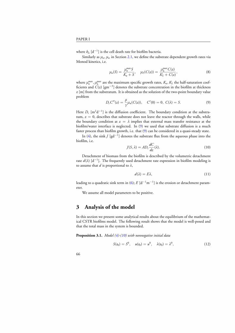
PAPER I
where kl [d−1] is the cell death rate for biofilm bacteria.Similarly as μu, μw in Section 2.1, we define the substrate dependent growth rates via
Monod kinetics, i.e.
μu(S) =μ
maxu S
Ku + S, μl(C (z)) =
μmaxl C (z)
Kl + C (z), (8)
where μmaxu , μmax
l are the maximum specific growth rates, Ku,Kl the half-saturation coef-ficients and C (z) [gm−3] denotes the substrate concentration in the biofilm at thicknessz [m] from the substratum. It is obtained as the solution of the two-point boundary valueproblem
DcC ′′(z) =ρ
γμl(C (z)), C ′(0) = 0, C (λ) = S. (9)
Here Dc [m2d−1] is the diffusion coefficient. The boundary condition at the substra-tum, z = 0, describes that substrate does not leave the reactor through the walls, whilethe boundary condition at z = λ implies that external mass transfer resistance at thebiofilm/water interface is neglected. In (9) we used that substrate diffusion is a muchfaster process than biofilm growth, i.e. that (9) can be considered in a quasi-steady state.
In (4), the sink J [gd−1] denotes the substrate flux from the aqueous phase into thebiofilm, i.e.
J (S, λ) = ADcdCdz
(λ). (10)
Detachment of biomass from the biofilm is described by the volumetric detachmentrate d (λ) [d−1]. The frequently used detachment rate expression in biofilm modeling isto assume that d is proportional to λ,
d (λ) = Eλ, (11)
leading to a quadratic sink term in (6); E [d−1m−1] is the erosion or detachment param-eter.
We assume all model parameters to be positive.
3 Analysis of the model
In this section we present some analytical results about the equilibrium of the mathemat-ical CSTR biofilms model. The following result shows that the model is well-posed andthat the total mass in the system is bounded.
Proposition 3.1. Model (4)-(10) with nonnegative initial data
S(t0) = S0, u(t0) = u0, λ(t0) = λ0, (12)
66

PAPER I
possesses a unique, non-negative solution that exists for all t > 0 and satisfies
V γS(t) + u(t) + Aρλ(t) ≤ a + bt (13)
where a, b depend on model parameters and initial data.
Proof. First we formally re-write our model as an ordinary initial value problem. Notethat integrating (9) once and using the boundary conditions gives
dCdz
(λ) =ρ
γDc
ˆ l
0μl(C (z))dz. (14)
We define
j(λ, S) :=
{rgDc
´ l0 μl(C (z))dz, λ > 0
0 λ = 0.(15)
Note that C (z) is indirectly a function of S due to the boundary condition in (9), thereforealso j is a function of S. Then (4)-(10) becomes
S = D(Sin − S)− 1V
(uμu(S)γ
+ ADcj(λ, S))
(16)
u = u(μu(S)− D− ku) + Aρd (λ)λ− αu (17)
λ =γDc
ρj(λ, S)− λkl +
αuAρ− d (λ)λ. (18)
Some properties of the function j(λ, S) are summarized in Lemma 3.3 below. In particularwe note that j(0, ·) = 0 and j(·, 0) = 0. Thus using the tangent criterion, see [28], itfollows that the non-negative cone is positively invariant. Moreover, in the non-negativecone, the right hand sides of (16)-(18) are continuously differentiable, so the systemsatisfies a Lipschitz condition. This implies the local existence and uniqueness of a non-negative solution of the initial value problem with non-negative initial data.
Furthermore, adding the equations (16)-(18) gives the estimate
V γS + u + Aρλ = Qγ(Sin − S)− uD− uku − Aρλkl ≤ QγSin.
ThusV γS(t) + u(t) + Aρλ(t) ≤ V γS0 + u0 + Aρλ0 + QγSint.
Therefore, since S, u, λ are non-negative, they exist and are bounded by a positive linearfunction for every t > 0.
Remark 3.2. It is easily verified through eqs. (5) and (6) that all solutions S, u, λ to theinitial value problem (4)-(6) are such that either u = λ = 0 or u > 0, λ > 0 for all t.
67
PAPER I
Thus, if biomass is not absent from the system, it exists simultaneously in suspended andwall attached form.
In the following lemma we derive a result that will be used later on in the stabilityanalysis.
Lemma 3.3. The function j(λ, S) for λ ≥ 0, S ≥ 0 is well-defined, nonnegative anddifferentiable. It has the following properties:
(a) j(·, 0) = 0, j(0, ·) = 0,
(b) ∂j∂S (0, S) = 0,
(c)Sθ
Kl + S≤ ∂j
∂λ(0, S) ≤ Sθ
Kl
, (19)
where θ =rmmax
l
gDcand Kl is the half-saturation coefficient from (8).
Proof. The function j(λ, S) is well-defined since the boundary value problem (9) has aunique solution. If λ and S are positive, this solution is positive; since C (z) is differen-tiable with respect to the parameters λ and S, also j(λ, S) is.
(a) For S = 0 we have C (λ) = 0 from the boundary conditions in (9). Since C (z) is acontinuous nonnegative function we have C (z) ≡ 0⇒ μl(C (z)) ≡ 0⇒ j(·, 0) =0.
(b) The derivative of j with respect to S for λ = 0 is by definition
∂j∂S
(0, S) = limh→0
j(0, S + h)− j(0, S)h
(a)= 0.
(c) We non-dimensionalize (9) with x = z/λ and c(z) = C (z)/S. The equation nowbecomes
c′′(x) = λ2 ρμmaxl
γDc
c(x)Kl + Sc(x)
, (20)
0 < x < 1, c′(0) = 0, c(1) = 1.
Further, we consider the two linear auxiliary problems
c′′(x) = θλ2 c(x)Kl + S
(21)
68

PAPER I
and
c′′(x) = θλ2 c(x)Kl
, (22)
with the same boundary conditions as in (20), where θ =rmmax
l
gDc. The solution c(x)
of (20) is continuous and bounded by 0 < c(x) < 1. Therefore Kl < Kl + cS <Kl + S. We denote the solutions to (21) and (22) by c1 and c2 respectively. Withcomparison theorems for Sturm-Liouville type boundary value problems, e.g. [28],we get
c1(x) ≥ c(x) ≥ c2(x) (23)
for all 0 < x < 1. Since c1(1) = c(1) = c2(1) = 1 we conclude that
c′1(1) ≤ c′(1) ≤ c′2(1). (24)
By reversing the non-dimensionalization, we obtain c′(1) = lS C ′(λ) and with (14)
and (15) from (24)j1(λ, S) ≤ j(λ, S) ≤ j2(λ, S), (25)
where j1 and j2 are defined in analogy with (15) for the estimates c1 and c2. For afixed S, j1(0, S) = j(0, S) = j2(0, S) = 0 together with (25) gives us
∂j1∂λ
(0, S) ≤ ∂j∂λ
(0, S) ≤ ∂j2∂λ
(0, S). (26)
The solution to (21) is
c1(x) = B1(λ, S)(
ex√j1(l,S) + e−x
√j1(l,S)
)(27)
with θ1(λ, S) = jl2
Kl+S and B1(λ, S) =(
e√j1(l,S) + e−
√j1(l,S)
)−1. Similarly, the
solution to (22) is
c2(x) = B2(λ)(
ex√j2(l) + e−x
√j2(l)
)(28)
with θ2(λ) = jl2
Kland B2(λ) =
(e√j2(l) + e−
√j2(l)
)−1. The fluxes are now
j1(λ, S) = SB1(λ, S)
√θ
Kl + S
(el√
j
Kl+S − e
−l√
j
Kl+S
), (29)
j2(λ, S) = SB2(λ)
√θ
Kl
(el√
j
Kl − e
−l√
j
Kl
)(30)
69
PAPER I
with
∂j1∂λ
(λ, S) =SθB1(λ, S)
Kl + S
(el√
j
Kl+S − e
−l√
j
Kl+S
), (31)
∂j2∂λ
(λ, S) =SθB2(λ)
Kl
(el√
j
Kl − e
−l√
j
Kl
)(32)
which gives us
∂j1∂λ
(0, S) =2SθB1(0, S)
Kl + S=
SθKl + S
, (33)
∂j2∂λ
(0, S) =2SθB2(0)
Kl
=SθKl
. (34)
The assertion follows from (26).
Remark 3.4. We observe that the estimates of j(λ, S) are in fact
j1(λ, S) = S
√θ
Kl + Stanh
√λ2θ
Kl + S, (35)
j2(λ, S) = S
√θ
Kl
tanh
√λ2θ
Kl
, (36)
with θ =rmmax
l
gDcand j1(λ, S) ≤ j(λ, S) ≤ j2(λ, S), where j1, j2 are the substrate fluxes of
limiting first-order kinetic models. An illustration for S = 10 g/m3 is given in Figure1. An improved upper estimate for j for small enough λ could be obtained from thezero-order kinetics problem
c′′(x) =θS
Kl + S,
which leads to a linear function in λ, see also [1].
Proposition 3.5. Let α > 0 and d (λ) > 0. Then for the system of equations (4)-(6) thewashout equilibrium E0 = (Sin, 0, 0) exists for all parameters. It is asymptotically stable if
μu(Sin) < D + ku + α and∂j∂λ
(0, Sin) <klργDc
70

PAPER I
0 0.2 0.4 0.6 0.8 1
x 10−3
0
5
10
15
x 104
λ (m)
j (g/
m4 )
lower bound j1(λ,10)
j(λ,10)upper bound j
2(λ,10)
Figure 1: Numerical approximation of j(λ, 10) with its upper (yellow dashed) and lower(black solid) bound using parameters from Tables 1 and 2.
and unstable if either
μu(Sin) > D + ku + α or∂j∂λ
(0, Sin) >klργDc
.
Proof. It is easily verified that the trivial equilibrium E0 = (Sin, 0, 0) always exists. Todetermine the stability of the equilibrium we calculate the Jacobian J (S, u, λ) of the righthand side of (16)-(18)−D− um′u(S)
Vg − ADcV
∂j∂S (λ, S) −mu(S)
Vg −ADcV
∂j∂l (λ, S)
uμ′u(S) μu(S)− D− ku − α Aρ(d (λ) + λd ′(λ))gDcr
∂j∂S (λ, S) a
ArgDcr
∂j∂l (λ, S)− (d (λ) + λd ′(λ))− kl
which for E0 simplifies to
J (Sin, 0, 0) =
−D −mu(Sin)Vg −ADc
V∂j∂l (0, Sin)
0 μu(Sin)− D− ku − α 00 a
ArgDcr
∂j∂l (0, Sin)− kl
.
71
PAPER I
The eigenvalues of J (Sin, 0, 0) are
σ1 = −D,
σ2 = μu(Sin)− D− ku − α,
σ3 =γDc
ρ
∂j∂λ
(0, Sin)− kl.
For asymptotic stability we need all eigenvalues to be negative. From this follows theassertion.
The function j(λ, S) and its derivatives are not easy to evaluate. Instead, using theestimates from Lemma 3.3, we can derive the following weaker criterion
Corollary 3.6. A sufficient condition for asymptotic stability of the trivial equilibrium E0 =(Sin, 0, 0) is
μu(Sin) < D + ku + α andSin
Kl
<klμ
maxl
.
On the other hand,
μu(Sin) > D + ku + α orSin
Kl + Sin >klμ
maxl
is sufficient for instability.
Observe that the stability criterion in Corollary 3.6 consists of two parts. One refersto the suspended biomass only and presents the classical persistence criterion where apopulation will not establish if the growth rate is smaller than the sum of dilution anddeath rate. The second criterion only refers to the biofilm: this stability and instabilityresult is independent of the reactor flow rate and of the detachment rate coefficient E , inagreement with the analysis of [3].
Figure 2 illustrates the numerical approximation of ∂j∂l (0, Sin) with its upper and
lower estimate. We observe that the approximation of ∂j∂l (0, Sin) corresponds to the lower
estimate rmmaxl
Sin
gDc (Kl+Sin) . This is in good agreement with the results of [1], where an analytical
approximation of the form j(λ, S) ≈ const · lSKl+S was derived with a Homotopy Pertur-
bation Method argument, which could be numerically verified for an extended range ofbiofilm parameters. Stability of the trivial equilibrium E0 is attained for Sin such that∂j∂l (0, Sin) lies beneath klr
gDc, which is represented by the dotted line in Figure 2.
In summary, with Proposition 3.1 we determine the existence of a unique, non-negative solution to our model (4)-(10), introducing the function j(λ, S) in (15) and
72
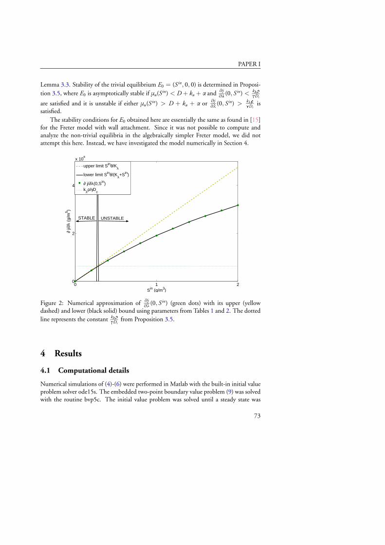
PAPER I
Lemma 3.3. Stability of the trivial equilibrium E0 = (Sin, 0, 0) is determined in Proposi-tion 3.5, where E0 is asymptotically stable if μu(Sin) < D + ku + α and ∂j
∂l (0, Sin) < klrgDc
are satisfied and it is unstable if either μu(Sin) > D + ku + α or ∂j∂l (0, Sin) > klr
gDcis
satisfied.The stability conditions for E0 obtained here are essentially the same as found in [15]
for the Freter model with wall attachment. Since it was not possible to compute andanalyze the non-trivial equilibria in the algebraically simpler Freter model, we did notattempt this here. Instead, we have investigated the model numerically in Section 4.
0 1 20
2
4
x 108
Sin (g/m3)
∂ j/∂
λ (g
/m5 )
upper limit Sinθ/Kλ
lower limit Sinθ/(Kλ+Sin)
∂ j/∂λ(0,Sin)kλρ/γD
c
STABLE UNSTABLE
Figure 2: Numerical approximation of ∂j∂l (0, Sin) (green dots) with its upper (yellow
dashed) and lower (black solid) bound using parameters from Tables 1 and 2. The dottedline represents the constant klr
gDcfrom Proposition 3.5.
4 Results
4.1 Computational details
Numerical simulations of (4)-(6) were performed in Matlab with the built-in initial valueproblem solver ode15s. The embedded two-point boundary value problem (9) was solvedwith the routine bvp5c. The initial value problem was solved until a steady state was
73

PAPER I
reached upon which the simulations were terminated. The initial conditions were
S(0) = Sin g/m3, u(0) = 10−6 g, λ(0) = 0 m,
where the reactor parameter Sin was varied together with colonizable surface area A anddilution rate D. This specific choice for S(0) implies that the medium that is added to thereactor is the same as the medium with which the reactor is initially filled, which seems areasonable assumption. Assuming a cylindrical reactor with dimensions specified in Table1 we have a volume V ≈ 0.00118 m3 and an inner surface area Areactor ≈ 0.055 m2. Thesurface area A can be increased by adding suspended carriers on which biofilms can form[17], i.e. we always have A ≥ Areactor.
Table 1: Reactor dimensions.
Parameter Value Referenceradius 0.05 m assumedheight 0.15 m assumedsuspended carrier area 0.0068 m2/carrier [17]
The model parameters are summarized in Table 2. To allow better comparison, weused the same growth parameter values for both biofilm and suspended biomass, i.e. weinterpret the latter as microbial flocs, i.e. bacterial communities without substratum. Thespecific choices of model parameters are taken from Benchmark Problem 1 of the Inter-national Water Association’s Taskgroup on Biofilm Modelling, i.e. our reactor models asufficiently aerated system in which carbon is the only growth limiting substrate.
The values for the attachment rate α and erosion parameter E were assumed. Theerosion parameter E was chosen large enough so that the results from our 1D modelcould be comparable to the results from a 2D model, as shown by [31]. In their study theauthors investigate values ranging from E = 22.8/d to E = 2280/d and show that thebiofilm thickness λ(t) originating from a 1D model is very different from λ(t) from a 2Dmodel for small values of E and very similar for large values of E . We picked a value in themiddle of the range tested by these authors, which however can be viewed at the higherend of the range used by other authors. Of all the processes considered in our model,biofilm attachment is probably the least understood one. Also here we choose a relativelyhigh value, assuming that one bacterium attaches to the wall for every six bacteria thatgrow in the bulk liquid.
4.2 Typical simulations
We solved (4)-(10) numerically, stopping the simulations once the solutions had attainedsteady state. In accordance with our analysis, two steady state forms were observed, de-
74
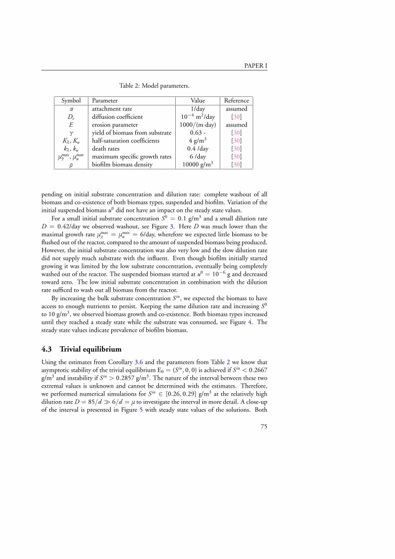
PAPER I
Table 2: Model parameters.
Symbol Parameter Value Referenceα attachment rate 1/day assumed
Dc diffusion coefficient 10−4 m2/day [30]E erosion parameter 1000/(m·day) assumedγ yield of biomass from substrate 0.63 - [30]
Kl, Ku half-saturation coefficients 4 g/m3 [30]kl, ku death rates 0.4 /day [30]μ
maxl , μmax
u maximum specific growth rates 6 /day [30]ρ biofilm biomass density 10000 g/m3 [30]
pending on initial substrate concentration and dilution rate: complete washout of allbiomass and co-existence of both biomass types, suspended and biofilm. Variation of theinitial suspended biomass u0 did not have an impact on the steady state values.
For a small initial substrate concentration S0 = 0.1 g/m3 and a small dilution rateD = 0.42/day we observed washout, see Figure 3. Here D was much lower than themaximal growth rate μmax
l = μmaxu = 6/day, wherefore we expected little biomass to be
flushed out of the reactor, compared to the amount of suspended biomass being produced.However, the initial substrate concentration was also very low and the slow dilution ratedid not supply much substrate with the influent. Even though biofilm initially startedgrowing it was limited by the low substrate concentration, eventually being completelywashed out of the reactor. The suspended biomass started at u0 = 10−6 g and decreasedtoward zero. The low initial substrate concentration in combination with the dilutionrate sufficed to wash out all biomass from the reactor.
By increasing the bulk substrate concentration Sin, we expected the biomass to haveaccess to enough nutrients to persist. Keeping the same dilution rate and increasing S0
to 10 g/m3, we observed biomass growth and co-existence. Both biomass types increaseduntil they reached a steady state while the substrate was consumed, see Figure 4. Thesteady state values indicate prevalence of biofilm biomass.
4.3 Trivial equilibrium
Using the estimates from Corollary 3.6 and the parameters from Table 2 we know thatasymptotic stability of the trivial equilibrium E0 = (Sin, 0, 0) is achieved if Sin < 0.2667g/m3 and instability if Sin > 0.2857 g/m3. The nature of the interval between these twoextremal values is unknown and cannot be determined with the estimates. Therefore,we performed numerical simulations for Sin ∈ [0.26, 0.29] g/m3 at the relatively highdilution rate D = 85/d � 6/d = μ to investigate the interval in more detail. A close-upof the interval is presented in Figure 5 with steady state values of the solutions. Both
75
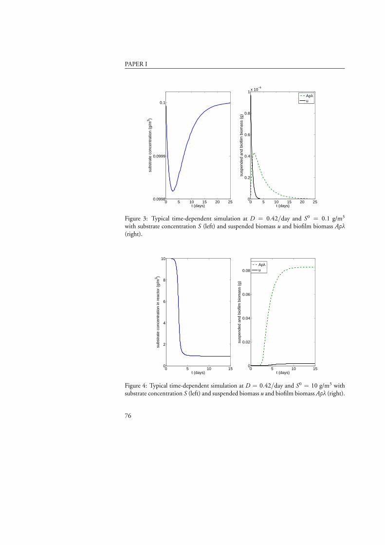
PAPER I
0 5 10 15 20 250.0998
0.0999
0.1
t (days)
subs
trat
e co
ncen
trat
ion
(g/m
3 )
0 5 10 15 20 250
0.2
0.4
0.6
0.8
1x 10
−6
t (days)
susp
ende
d an
d bi
ofilm
bio
mas
s (g
)
Aρλu
Figure 3: Typical time-dependent simulation at D = 0.42/day and S0 = 0.1 g/m3
with substrate concentration S (left) and suspended biomass u and biofilm biomass Aρλ(right).
0 5 10 150
2
4
6
8
10
t (days)
subs
trat
e co
ncen
trat
ion
in r
eact
or (
g/m
3 )
0 5 10 150
0.02
0.04
0.06
0.08
t (days)
susp
ende
d an
d bi
ofilm
bio
mas
s (g
)
Aρλu
Figure 4: Typical time-dependent simulation at D = 0.42/day and S0 = 10 g/m3 withsubstrate concentration S (left) and suspended biomass u and biofilm biomass Aρλ (right).
76

PAPER I
0,26 0,290
5
x 10−9
Sin (g/m3)
susp
ende
d bi
omas
s u
(g)
0.26 0.265 0.27 0.275 0.28 0.2850
5
x 10−4
biof
ilm b
iom
ass
Aρλ
(g)
Aρλu
Figure 5: Steady state values of suspended and biofilm biomass, on two different axes, forSin ∈ [0.26, 0.29] g/m3 at D = 85/day, showing a close-up of E0 becoming unstable.Two vertical dashed lines indicate the critical values given by Corollary 3.6.
biomass types were washed out for the lower values of Sin. The critical value of Sin, whenboth suspended and biofilm biomass are positive, was in fact closer to 0.2857 g/m3, givenby the upper bound in Corollary 3.6.
Led by the conclusions of Proposition 3.5 we were interested in the behavior of ourmodel for variations in parameters D and Sin. We rendered a coarse two dimensional gridand performed numerical simulations for 0 < Sin ≤ 1 g/m3 and 0 < D < 85 /day,presented in Figures 6 and 7. We expected impact on the stability of the trivial equilib-rium from both D and Sin, depending on the signs of the eigenvalues in Proposition 3.5.Our results, however, show that the stability was governed solely by Sin. Washout of allbiomass occurred for Sin < 0.3 g/m3, independent of the values of D. This is a valuemuch smaller than the half saturation concentration, i.e. indicates a regime of nutrientscarcity. The critical value of Sin for which the third eigenvalue σ3 becomes positive israther small. In this range of Sin, the second eigenvalue σ2 remains negative, implyingthat σ3 is always the first eigenvalue to become positive as Sin varies. Since D is not a partof the expression for σ3, the stability of E0 is governed by the reaction processes only, butdoes not depend on the bulk hydrodynamics. An increase in Sin beyond the critical valuecaused instability of E0 expressed by an increase in biomass.
77

PAPER I
0
0.5
1
030
6090
0
0.025
0.05
Sin (g/m3)D (1/day)
biof
ilm b
iom
ass
(g)
0
0.5
1
0
30
60
900
3
6
x 10−5
Sin (g/m3)D (1/day)
susp
ende
d bi
omas
s (g
)
0
0.025
0.05
0
3
6x 10
−5
Figure 6: Suspended biomass u (left) and biofilm biomass Aρλ (right) at steady stateas functions of the dilution rate D and the initial substrate concentration Sin. Trivialequilibrium E0 = (Sin, 0, 0) marked in dark blue.
00.2
0.40.6
0.81
0
30
60
900
0.2
0.4
0.6
Sin (g/m3)D (1/day)
subs
trat
e co
ncen
trat
ion
in r
eact
or (
g/m
3 )
0.25
0.5
Figure 7: Substrate concentration S in the reactor at steady state as function of the dilu-tion rate D and the initial substrate concentration Sin. Trivial equilibrium E0 = (Sin, 0, 0)marked in dark blue with white circles.
78

PAPER I
0 20 40 60 80 1000
0.5
1
1.5
2
2.5x 10
−3
D (1/day)
susp
ende
d bi
omas
s (g
)
0 20 40 60 80 1000
0.05
0.1
0.15
0.2
0.25
D (1/day)
biof
ilm b
iom
ass
(g)
Sin=10
Sin=7
Sin=4
Sin=10
Sin=7
Sin=4
Figure 8: Suspended biomass u (left) and biofilm biomass Aρλ (right) at steady state asfunctions of the dilution rate D at Sin = 10, 7 and 4 g/m3.
4.4 Persistence equilibrium
We know from Proposition 3.5 that the trivial equilibrium is unstable, i.e. S, u, λ > 0,when Sin is large enough. Therefore, the longterm behavior of the model was investigatednumerically through variation of Sin and D. Washout occurred for Sin < 0.3 g/m3, aspreviously discussed. Persistence of both biomass types was achieved in every simulationfor Sin ≥ 0.3 g/m3. The two biomass types behaved differently as Sin and D varied.Suspended biomass increased in the lower range of D while the dilution rate was stillcomparable to the growth rate. But as D rose to multiples of μmax
u = 6/day it acted asthe stronger force, wherefore more suspended biomass was washed out before it couldnotably contribute to suspended growth. Eventually, for very large D, there was very littlesuspended biomass in the reactor, however never vanishing completely. An increase in Sin
increased the peak of suspended biomass before it declined due to washout. Figure 8 is asnapshot of steady states of u and Aρλ at Sin = 4, 7 and 10 g/m3 as they vary along D.Biofilm biomass increased for both Sin and D, eventually reaching a plateau for large D.
Figure 8 indicates that the suspended biomass will decrease eventually as D increases,whereas the biofilm will persist and, in fact, keep growing. Larger D brings more nutrientsto the reactor wherefore the biofilm thickness increases. Since the detachment rate (11)has no connection to the dilution rate, it is not affected by variation in D. Eventually,suspended biomass will decrease to a minimum due to washout from the reactor for alarge enough dilution rate.
In our model (4)-(6), the bulk flow rate contributes to substrate supply and to washout
79
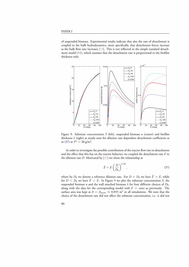
PAPER I
of suspended biomass. Experimental results indicate that also the rate of detachment iscoupled to the bulk hydrodynamics, more specifically, that detachment forces increaseas the bulk flow rate increases [19]. This is not reflected in the simple standard detach-ment model (11), which assumes that the detachment rate is proportional to the biofilmthickness only.
0 20 40 60 80 1000
5
10
15
20
25
D (1/day)
subs
trat
e in
rea
ctor
(g/
m3 )
D0=1
D0=10
D0=40
D0=100
E=1000
0 20 40 60 80 1000
0.005
0.01
0.015
D (1/day)
susp
ende
d bi
omas
s (g
)
D
0=1
D0=10
D0=40
D0=100
E=1000
0 20 40 60 80 1000
0.5
1x 10
−3
D (1/day)
biof
ilm th
ickn
ess
(m)
D0=1
D0=10
D0=40
D0=100
E=1000
Figure 9: Substrate concentration S (left), suspended biomass u (center) and biofilmthickness λ (right) at steady state for dilution rate dependent detachment coefficients asin (37) at Sin = 30 g/m3.
In order to investigate the possible contribution of the reactor flow rate to detachmentand the effect that this has on the reactor behavior, we coupled the detachment rate E tothe dilution rate D. Motivated by [22] we chose the relationship as
E = E(
DD0
)0.58
, (37)
where by D0 we denote a reference dilution rate. For D > D0 we have E > E , whilefor D < D0 we have E < E . In Figure 9 we plot the substrate concentration S, thesuspended biomass u and the wall attached biomass λ for four different choices of D0,along with the data for the corresponding model with E = const as previously. Thesurface area was kept at A = Areactor ≈ 0.055 m2 in all simulations. We note that thechoice of the detachment rate did not affect the substrate concentration, i.e. it did not
80
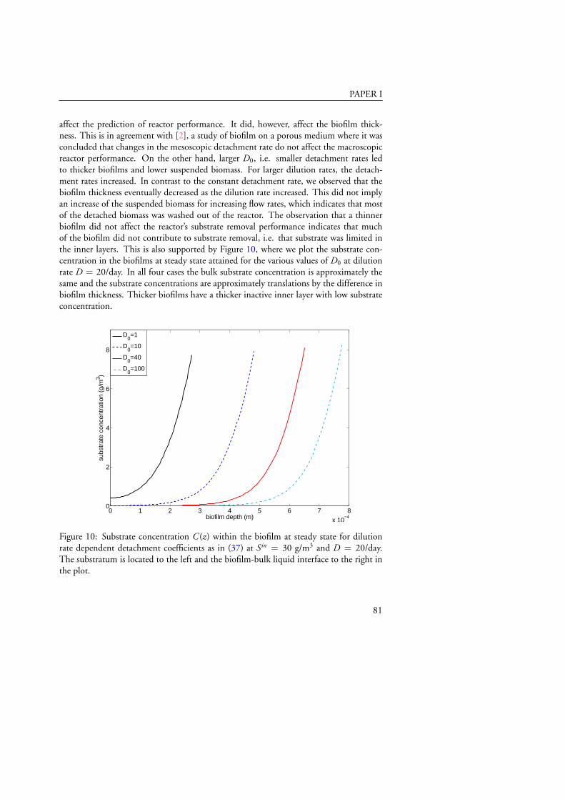
PAPER I
affect the prediction of reactor performance. It did, however, affect the biofilm thick-ness. This is in agreement with [2], a study of biofilm on a porous medium where it wasconcluded that changes in the mesoscopic detachment rate do not affect the macroscopicreactor performance. On the other hand, larger D0, i.e. smaller detachment rates ledto thicker biofilms and lower suspended biomass. For larger dilution rates, the detach-ment rates increased. In contrast to the constant detachment rate, we observed that thebiofilm thickness eventually decreased as the dilution rate increased. This did not implyan increase of the suspended biomass for increasing flow rates, which indicates that mostof the detached biomass was washed out of the reactor. The observation that a thinnerbiofilm did not affect the reactor’s substrate removal performance indicates that muchof the biofilm did not contribute to substrate removal, i.e. that substrate was limited inthe inner layers. This is also supported by Figure 10, where we plot the substrate con-centration in the biofilms at steady state attained for the various values of D0 at dilutionrate D = 20/day. In all four cases the bulk substrate concentration is approximately thesame and the substrate concentrations are approximately translations by the difference inbiofilm thickness. Thicker biofilms have a thicker inactive inner layer with low substrateconcentration.
0 1 2 3 4 5 6 7 8
x 10−4
0
2
4
6
8
biofilm depth (m)
subs
trat
e co
ncen
trat
ion
(g/m
3 )
D0=1
D0=10
D0=40
D0=100
Figure 10: Substrate concentration C (z) within the biofilm at steady state for dilutionrate dependent detachment coefficients as in (37) at Sin = 30 g/m3 and D = 20/day.The substratum is located to the left and the biofilm-bulk liquid interface to the right inthe plot.
81
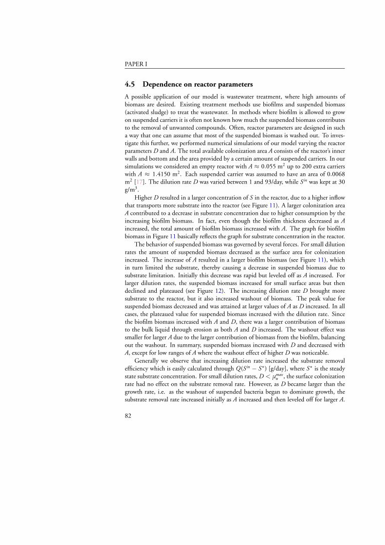
PAPER I
4.5 Dependence on reactor parameters
A possible application of our model is wastewater treatment, where high amounts ofbiomass are desired. Existing treatment methods use biofilms and suspended biomass(activated sludge) to treat the wastewater. In methods where biofilm is allowed to growon suspended carriers it is often not known how much the suspended biomass contributesto the removal of unwanted compounds. Often, reactor parameters are designed in sucha way that one can assume that most of the suspended biomass is washed out. To inves-tigate this further, we performed numerical simulations of our model varying the reactorparameters D and A. The total available colonization area A consists of the reactor’s innerwalls and bottom and the area provided by a certain amount of suspended carriers. In oursimulations we considered an empty reactor with A ≈ 0.055 m2 up to 200 extra carrierswith A ≈ 1.4150 m2. Each suspended carrier was assumed to have an area of 0.0068m2 [17]. The dilution rate D was varied between 1 and 93/day, while Sin was kept at 30g/m3.
Higher D resulted in a larger concentration of S in the reactor, due to a higher inflowthat transports more substrate into the reactor (see Figure 11). A larger colonization areaA contributed to a decrease in substrate concentration due to higher consumption by theincreasing biofilm biomass. In fact, even though the biofilm thickness decreased as Aincreased, the total amount of biofilm biomass increased with A. The graph for biofilmbiomass in Figure 11 basically reflects the graph for substrate concentration in the reactor.
The behavior of suspended biomass was governed by several forces. For small dilutionrates the amount of suspended biomass decreased as the surface area for colonizationincreased. The increase of A resulted in a larger biofilm biomass (see Figure 11), whichin turn limited the substrate, thereby causing a decrease in suspended biomass due tosubstrate limitation. Initially this decrease was rapid but leveled off as A increased. Forlarger dilution rates, the suspended biomass increased for small surface areas but thendeclined and plateaued (see Figure 12). The increasing dilution rate D brought moresubstrate to the reactor, but it also increased washout of biomass. The peak value forsuspended biomass decreased and was attained at larger values of A as D increased. In allcases, the plateaued value for suspended biomass increased with the dilution rate. Sincethe biofilm biomass increased with A and D, there was a larger contribution of biomassto the bulk liquid through erosion as both A and D increased. The washout effect wassmaller for larger A due to the larger contribution of biomass from the biofilm, balancingout the washout. In summary, suspended biomass increased with D and decreased withA, except for low ranges of A where the washout effect of higher D was noticeable.
Generally we observe that increasing dilution rate increased the substrate removalefficiency which is easily calculated through Q(Sin − S∗) [g/day], where S∗ is the steadystate substrate concentration. For small dilution rates, D < μmax
u , the surface colonizationrate had no effect on the substrate removal rate. However, as D became larger than thegrowth rate, i.e. as the washout of suspended bacteria began to dominate growth, thesubstrate removal rate increased initially as A increased and then leveled off for larger A.
82
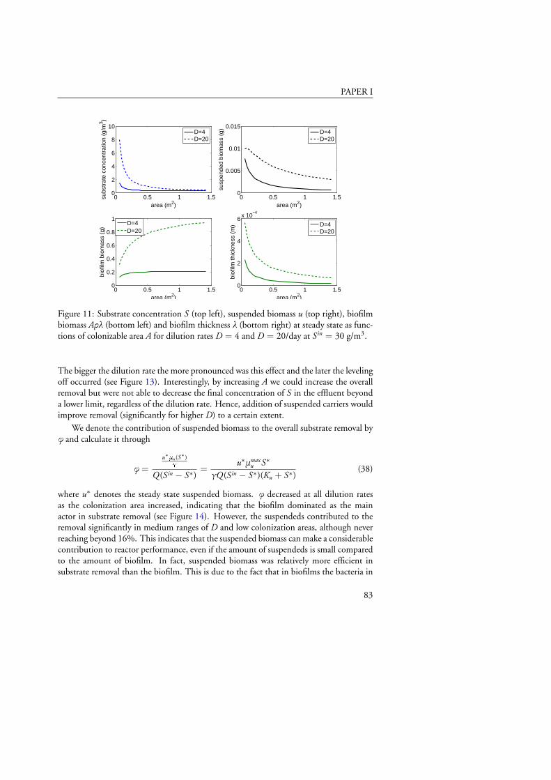
PAPER I
0 0.5 1 1.50
2
4
6
8
10
area (m2)
subs
trat
e co
ncen
trat
ion
(g/m
3 )
D=4D=20
0 0.5 1 1.50
0.005
0.01
0.015
area (m2)
susp
ende
d bi
omas
s (g
)
D=4D=20
0 0.5 1 1.50
0.2
0.4
0.6
0.8
1
area (m2)
biof
ilm b
iom
ass
(g)
D=4D=20
0 0.5 1 1.50
2
4
6x 10
−4
area (m2)
biof
ilm th
ickn
ess
(m)
D=4D=20
Figure 11: Substrate concentration S (top left), suspended biomass u (top right), biofilmbiomass Aρλ (bottom left) and biofilm thickness λ (bottom right) at steady state as func-tions of colonizable area A for dilution rates D = 4 and D = 20/day at Sin = 30 g/m3.
The bigger the dilution rate the more pronounced was this effect and the later the levelingoff occurred (see Figure 13). Interestingly, by increasing A we could increase the overallremoval but were not able to decrease the final concentration of S in the effluent beyonda lower limit, regardless of the dilution rate. Hence, addition of suspended carriers wouldimprove removal (significantly for higher D) to a certain extent.
We denote the contribution of suspended biomass to the overall substrate removal byφ and calculate it through
φ =
u∗mu(S∗)g
Q(Sin − S∗)=
u∗μmaxu S∗
γQ(Sin − S∗)(Ku + S∗)(38)
where u∗ denotes the steady state suspended biomass. φ decreased at all dilution ratesas the colonization area increased, indicating that the biofilm dominated as the mainactor in substrate removal (see Figure 14). However, the suspendeds contributed to theremoval significantly in medium ranges of D and low colonization areas, although neverreaching beyond 16%. This indicates that the suspended biomass can make a considerablecontribution to reactor performance, even if the amount of suspendeds is small comparedto the amount of biofilm. In fact, suspended biomass was relatively more efficient insubstrate removal than the biofilm. This is due to the fact that in biofilms the bacteria in
83
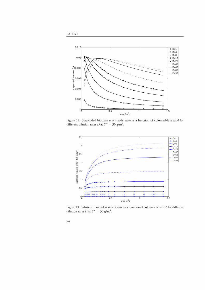
PAPER I
0 0.5 1 1.50
0.002
0.004
0.006
0.008
0.01
0.012
area (m2)
susp
ende
d bi
omas
s (g
)
D=1D=4D=8D=17D=25D=42D=68D=85D=93
Figure 12: Suspended biomass u at steady state as a function of colonizable area A fordifferent dilution rates D at Sin = 30 g/m3.
0 0.5 1 1.50
0.5
1
1.5
2
2.5
3
3.5
area (m2)
subs
trat
e re
mov
al Q
(Sin
−S
* ) (g
/day
)
D=1D=4D=8D=17D=25D=42D=68D=85D=93
Figure 13: Substrate removal at steady state as a function of colonizable area A for differentdilution rates D at Sin = 30 g/m3.
84

PAPER I
0 0.5 1 1.50
2
4
6
8
10
12
14
16
area (m2)
port
ion
of s
ubst
rate
rem
oval
per
form
ed b
y su
spen
ded
biom
ass
(%)
0 0.5 1 1.50
1
2
3
4
5
6
area (m2)
susp
ende
d bi
omas
s re
lativ
e to
tota
l bio
mas
s (%
)
D=1D=4D=8D=17D=25D=42D=68D=85D=93
D=1D=4D=8D=17D=25D=42D=68D=85D=93
Figure 14: Percentage of substrate removal performed by suspended biomass (left) andamount of suspended biomass relative to total biomass (right), at steady state as a functionof colonizable area A for different dilution rates D at Sin = 30 g/m3.
the inner layers often, particularly in thick biofilms, live under nutrient limitations anddo not contribute greatly to substrate degradation. φ corresponded to the behavior of thesuspended biomass for the different dilution rates, i.e. it increased initially in the lowerranges of D until it reached a peak and subsequently decreased due to higher washout.
5 Conclusion
In this paper we studied a mathematical model of bacterial population and resource dy-namics in a CSTR with wall attachment. This is a modification of Freter’s model, inwhich we treat the wall attached bacteria as biofilms. The resulting mathematical modelis more complex than the original Freter model, because the reactor mass balance is cou-pled with a diffusion-reaction equation for the substrate in the biofilm. The added alge-braic and physical complexity did not add increased dynamic complexity. The stabilityconditions for the trivial equilibrium of the modified model are essentially the same as forthe original Freter model. If the trivial equilibrium is unstable, the system attains a non-trivial equilibrium, in which both suspended and biofilm biomass co-exist. Overall, themodel shows a preference of the biomass for the biofilm mode of growth, as also observedin natural systems. In particular for large reactor flow rates suspended biomass is washed
85
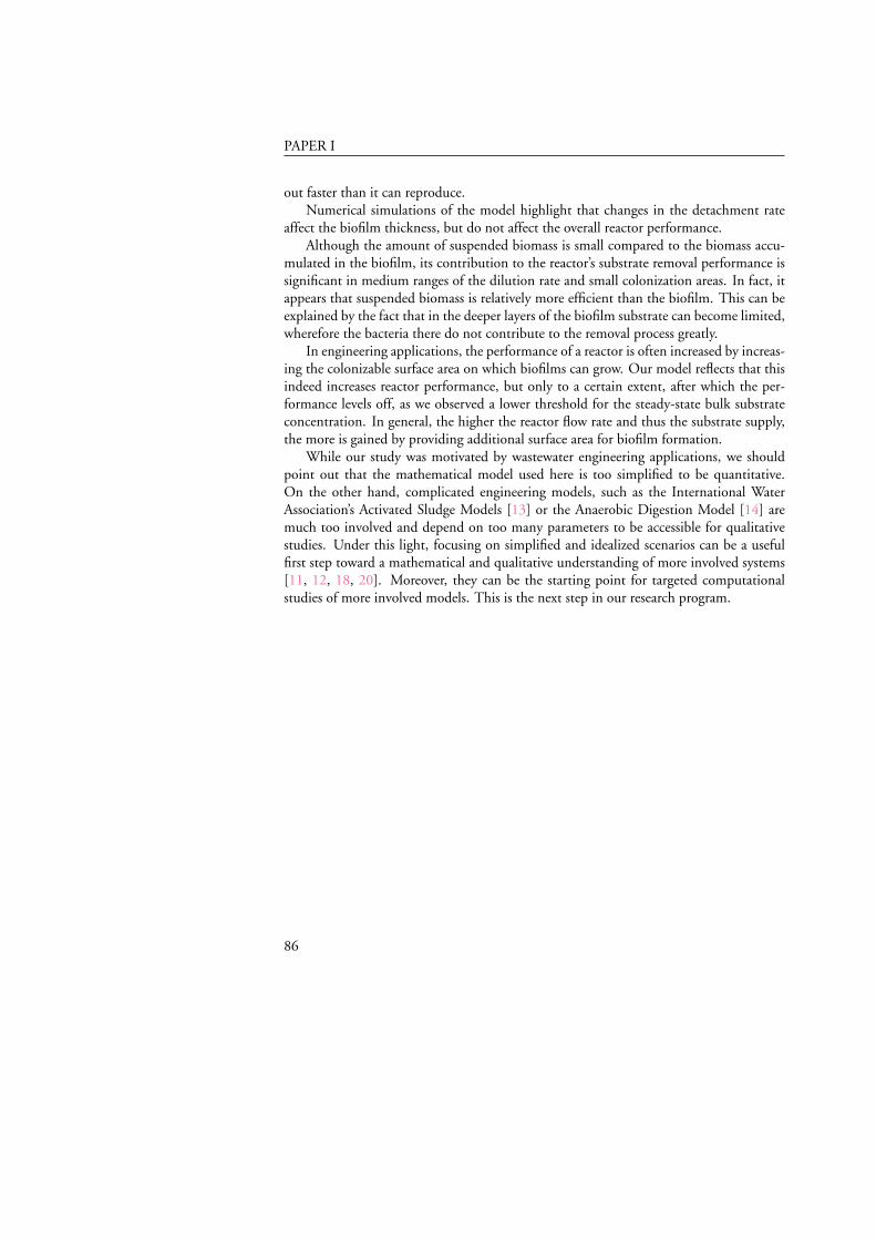
PAPER I
out faster than it can reproduce.Numerical simulations of the model highlight that changes in the detachment rate
affect the biofilm thickness, but do not affect the overall reactor performance.Although the amount of suspended biomass is small compared to the biomass accu-
mulated in the biofilm, its contribution to the reactor’s substrate removal performance issignificant in medium ranges of the dilution rate and small colonization areas. In fact, itappears that suspended biomass is relatively more efficient than the biofilm. This can beexplained by the fact that in the deeper layers of the biofilm substrate can become limited,wherefore the bacteria there do not contribute to the removal process greatly.
In engineering applications, the performance of a reactor is often increased by increas-ing the colonizable surface area on which biofilms can grow. Our model reflects that thisindeed increases reactor performance, but only to a certain extent, after which the per-formance levels off, as we observed a lower threshold for the steady-state bulk substrateconcentration. In general, the higher the reactor flow rate and thus the substrate supply,the more is gained by providing additional surface area for biofilm formation.
While our study was motivated by wastewater engineering applications, we shouldpoint out that the mathematical model used here is too simplified to be quantitative.On the other hand, complicated engineering models, such as the International WaterAssociation’s Activated Sludge Models [13] or the Anaerobic Digestion Model [14] aremuch too involved and depend on too many parameters to be accessible for qualitativestudies. Under this light, focusing on simplified and idealized scenarios can be a usefulfirst step toward a mathematical and qualitative understanding of more involved systems[11, 12, 18, 20]. Moreover, they can be the starting point for targeted computationalstudies of more involved models. This is the next step in our research program.
86

PAPER I
NomenclatureA area (m2)au half-saturation Monod const. of suspended bacteria (Freter) (g/m3)aw half-saturation Monod const. of wall-attached bacteria (Freter) (g/m3)D dilution rate (1/day)Dc diffusion coefficient (m2/day)E erosion parameter (1/m·day)F flow (velocity) through the reactor (Freter) (m3/day)Kl half-saturation Monod constant of biofilm (g/m3)Ku half-saturation Monod constant of suspended bacteria (g/m3)kl death rate of biofilm (1/day)ku death rate of suspended bacteria (1/day)kw death rate of wall-attached bacteria in Freter model (1/day)mu maximum growth rate of suspended bacteria (Freter) (1/day)mw maximum growth rate of wall-attached bacteria (Freter) (1/day)Q flow (velocity) through the reactor (m3/day)S substrate concentration (g/m3)S in substrate concentration at inlet (g/m3)u suspended bacteria (g)u concentration of suspended bacteria (Freter) (g/m3)V volume of the reactor (m3)w areal biomass density of wall-attached bacteria (g/m2)wmax maximum areal biomass density of wall-attached bacteria (g/m2)W = w/wmax wall occupancy fraction (-)
Greeksa attachment rate (1/day)b detachment rate (Freter) (1/day)l biofilm thickness (m)mmaxl maximum growth rate of biofilm (1/day)
mmaxu maximum growth rate of suspended bacteria (1/day)
g yield (-)r biofilm biomass density (g/m3)
87

PAPER I
Bibliography
[1] F. Abbas and H.J. Eberl, (2011). Analytical flux approximation for the Monod boundary valueproblem. Appl. Math. Comp. 218(4):1484-1494.
[2] F. Abbas and H.J. Eberl, (accepted). Investigation of the role of mesoscale detachment rateexpressions in a macroscale model of a porous medium biofilm reactor. Int. J. Biomath. Biostats.[scheduled for 2(1), 2011]
[3] F. Abbas, R. Sudarsan and H.J. Eberl, (accepted). Longtime behavior of one-dimensionalbiofilm models with shear dependent detachment rates. Math. Biosc. Eng.
[4] M.M. Ballyk, D.A. Jones, and H.L. Smith, (2001). Microbial competition in reactors with wallattachment. Microbial Ecology 41(3):210-221.
[5] M.M. Ballyk, D.A. Jones, and H.L. Smith, (2008). The biofilm model of Freter: a review.In P. Magal, S. Ruan (eds), Structured population models in biology and epidemiology, SpringerLecture Notes in Mathematics Vol.1936.
[6] E. Bester, E.A. Edwards and G.M. Wolfaardt, (2009). Planktonic cell yield is linked to biofilmdevelopment. Can. J. Microbiology, 55(10):1195-1206.
[7] B. Boldin, (2008). Persistence and spread of gastro-intestinal infections: the case of enterotox-igenic Escherichia coli in piglets. B. Math. Biol., 70(7):2077-2101.
[8] J.W. Costerton, Z. Lewandowski, D.E. Caldwell, D.R. Korber and H.M. Lappin-Scott,(1995). Microbial Biofilms. Ann. Rev. Microbiology 49:711-745.
[9] H.C. Flemming, (2000). Biofilme – das Leben am Rande der Wasserphase Nachr. Chemie48:442-447.
[10] R. Freter, H. Brickner, J. Fekete, M. Vickerman and K. Carey, (1983). Survival and implan-tation of Escherichia coli in the intestinal tract. Infect. Immun. 39:686-703.
[11] E.V. Grigorieva and E.N. Khailov, (2010). Minimization of pollution concentration on agiven time interval for the waste water cleaning plant. J. Control Sci. Eng. vol. 2010, Article ID712794, 10 pages.
[12] M. El Hajji, F. Mazenc, and J. Harmand, (2010). A mathematical study of a syntrophicrelationship of a model of anaerobic digestion process. Math. Biosci. Eng. 7(3):641-656.
[13] M. Henze, W. Gujer, M. Takashi, and M. van Loosdrecht, (2002). Activated Sludge ModelsASM1, ASM2, ASM2d and ASM3. IWA Publishing.
[14] IWA Task Group, (2002). Anaerobic Digestion Model No. 1 (ADM1). IWA Publishing.
[15] D. Jones, H. V. Kojouharov, and D. Le, H. Smith, (2003). The Freter model: A simple modelof biofilm formation. Math. Bio. 47:137-152.
[16] Z. Lewandowski and H. Beyenal, (2007). Fundamentals of biofilm research. CRC Press, BocaRaton.
88
PAPER I
[17] A. Masic, J. Bengtsson, and M. Christensson, (2010). Measuring and modeling the oxygenprofile in a nitrifying Moving Bed Biofilm Reactor. Math. Biosci. 227:1-11.
[18] J. Moreno, (1999). Optimal time control of bioreactors for the wastewater treatment. Optim.Control Appl. Meth. 20:145-164.
[19] E. Morgenroth, (2003). Detachment: an often-overlooked phenomenon in biofilm researchand modeling. In: S. Wuertz et al (eds), Biofilms in Wastewater Treatment, pp 246-290, IWAPublishing, London.
[20] T.G. Müller, N. Noykova, M. Gyllenberg, and J. Timmer, (2002). Parameter identificationin dynamical models of anaerobic waste water treatment. Math. Biosci. 177-178:147-160.
[21] L.A. Pritchett and J.D. Dockery, (2001). Steady state solutions of a one-dimensional biofilmmodel. Math. Comput. Model. 33:255-263.
[22] B.E. Rittmann, (1982). The effect of shear stress on biofilm loss rate. Biotech. Bioeng. 24:501-506.
[23] B.E. Rittmann and P.L. McCarty, (2001). Environmental Biotechnology. McGraw-Hill.
[24] H.L. Smith and P. Waltman, (1995). The theory of the chemostat. Cambridge UniversityPress, Cambridge, UK.
[25] E.D. Stemmons and H.L. Smith, (2000). Competition in a chemostat with wall attachment.SIAM J. Appl. Math. 61(2):567-595.
[26] P.S. Stewart, (2003). Diffusion in biofilms. J. Bacteriol. 185(5):1485-1491.
[27] B. Szomolay, (2008). Analysis of a moving boundary value problem arising in biofilm model-ing. Math. Meth. Appl. Sci. 31:1835-1859.
[28] W. Walter, (2000). Gewöhnliche Differentialgleichungen. 7th ed, Springer-Verlag, Berlin.
[29] O. Wanner and W. Gujer, (1986). A multispecies biofilm model. Biotech. Bioeng. 28:314-328.
[30] O. Wanner, H. Eberl, E. Morgenroth, D.R. Noguera, C. Picioreanu, B. Rittmann, and M.van Loosdrecht, (2006). Mathematical modeling of biofilms, Scientific and Technical ReportNo.18. IWA Publishing.
[31] J.B. Xavier, C. Picioreanu, and M.C.M. van Loosdrecht, (2004). A modeling study of theactivity and structure of biofilms in biological reactors. Biofilms 1(4):377-391.
89
PAPER II
Published in Mathematical Biosciences 2010.
Measuring and modeling the oxygen profile in a nitrifying Moving BedBiofilm Reactor
Alma Mašic a,b,*, Jessica Bengtsson c, Magnus Christensson d
a Centre for Technological Studies, Malmö University, SE-20506 Malmö, Swedenb Centre for Mathematical Sciences, Lund University, Box 118, SE-22100, Lund, Swedenc Alfa Laval Copenhagen A/S, Maskinvej 5, DK-2860 Søborg, Denmarkd AnoxKaldnes AB, Klosterängsvägen 11A, SE-22647 Lund, Sweden
a r t i c l e i n f o
Article history:Received 27 August 2009Received in revised form 7 May 2010Accepted 16 May 2010Available online 24 May 2010
Keywords:Biofilm modelMicroelectrodeMBBRMoving Bed Biofilm ReactorNitrifying biofilmsOxygen profile
a b s t r a c t
In this paper we determine the oxygen profile in a biofilm on suspended carriers in two ways: firstly bymicroelectrode measurements and secondly by a simple mathematical model.
The Moving Bed Biofilm Reactor is well-established for wastewater treatment where bacteria grow as abiofilm on the protective surfaces of suspended carriers. The flat shaped BiofilmChip P was developed toallow good conditions for transport of substrates into the biofilm. The oxygen profile was measured in situthe nitrifying biofilm with a microelectrode and it was simulated with a one-dimensional mathematicalmodel. We extended the model by adding a CSTR equation, to connect the reactor to the biofilm throughthe boundary conditions.
We showed the dependence of the thickness of the mass transfer boundary layer on the bulk flow rate.Finally, we estimated the erosion parameter k to increase the concordance between the measured andsimulated profiles. This lead to a simple empirical relationship between k and the flow rate. The datagathered by in situ microelectrode measurements can, together with the mathematical model, be usedin predictive modeling and give more insight in the design of new carriers, with the ambition of makingprocess operation more energy efficient.
� 2010 Elsevier Inc. All rights reserved.
1. Introduction
The Moving Bed Biofilm Reactor (MBBR) is well-established forwastewater treatment where bacteria grow as a biofilm on the pro-tective surfaces of suspended carriers [19]. The reactor is aeratedand mixed through rising air bubbles from the bottom blowers.In nitrification, oxygen acts as an electron acceptor in the two-stepconversion of ammonium to nitrate:
Step 1 : 2NHþ4 þ 3O2�2NO�2 þ 4Hþ þ 2H2O;Step 2 : 2NO�2 þ O2�2NO�3 :
ð1Þ
The overall conversion rate is usually limited by the first step of thereaction, i.e. conversion of ammonium to nitrite [10, Section 3.4.4].In wastewater conditions, the availability of ammonium is generallymaintained on a high level due to influent water. In the presence ofa biofilm oxygen limitation occurs when [8]:
DO2 � SO2 < mNHþ4 ;O2� DNHþ4
� SNHþ4; ð2Þ
where DO2 ;DNHþ4are diffusion coefficients, mNHþ4 ;O2
is the stoichiome-tric coefficient of the overall ratio of oxygen consumption to ammo-nium removal and SO2 ; SNHþ4
are the bulk concentrations of oxygenand ammonium, respectively.
In a biofilm process, transport of oxygen through diffusion lim-its the nitrification rate to a larger degree compared to what isfound in a suspended biomass where convection is more signifi-cant. Previous studies on the AnoxKaldnes™ carrier media typeK1 have shown that the nitrification rate was close to first orderkinetics with respect to dissolved oxygen (DO) when oxygen limit-ing conditions were established [9]. To maintain a higher DO con-centration in the bulk liquid an increase in oxygen transfer fromthe air bubbles is required, obtained by supplying more air fromthe blowers, thereby increasing the energy demand per aeratedvolume. However, the total energy demand for a MBBR biologicalprocess operated at elevated DO concentration may not be higherthan for a biological process operated at a lower DO concentration,since less aerated volume is needed in the first case due to thehigher efficiency. A key factor in the development of new sus-pended carriers is then not only to increase the available protectivesurface area, thereby directly contributing to a larger biofilm, butalso to allow good conditions for transport of substrates into thebiofilm. The flat shaped AnoxKaldnes™ carrier media type
0025-5564/$ - see front matter � 2010 Elsevier Inc. All rights reserved.doi:10.1016/j.mbs.2010.05.004
* Corresponding author at: Centre for Technological Studies, Malmö University,SE-20506 Malmö, Sweden. Tel.: +46 40 6657738; fax: +46 40 6657646.
E-mail addresses: [email protected] (A. Mašic), [email protected] (J. Bengtsson), [email protected] (M. Christensson).
Mathematical Biosciences 227 (2010) 1–11
Contents lists available at ScienceDirect
Mathematical Biosciences
journal homepage: www.elsevier .com/locate /mbs
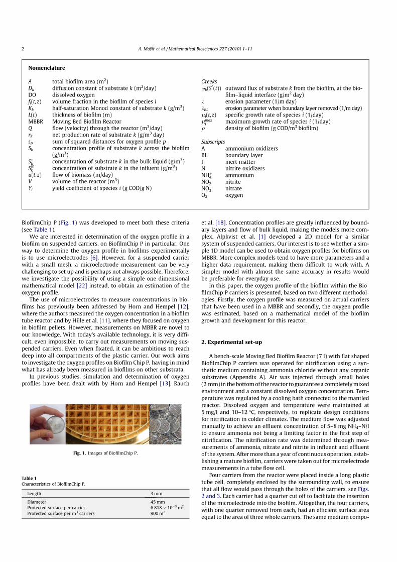
BiofilmChip P (Fig. 1) was developed to meet both these criteria(see Table 1).
We are interested in determination of the oxygen profile in abiofilm on suspended carriers, on BiofilmChip P in particular. Oneway to determine the oxygen profile in biofilms experimentallyis to use microelectrodes [6]. However, for a suspended carrierwith a small mesh, a microelectrode measurement can be verychallenging to set up and is perhaps not always possible. Therefore,we investigate the possibility of using a simple one-dimensionalmathematical model [22] instead, to obtain an estimation of theoxygen profile.
The use of microelectrodes to measure concentrations in bio-films has previously been addressed by Horn and Hempel [12],where the authors measured the oxygen concentration in a biofilmtube reactor and by Hille et al. [11], where they focused on oxygenin biofilm pellets. However, measurements on MBBR are novel toour knowledge. With today’s available technology, it is very diffi-cult, even impossible, to carry out measurements on moving sus-pended carriers. Even when fixated, it can be ambitious to reachdeep into all compartments of the plastic carrier. Our work aimsto investigate the oxygen profiles on Biofilm Chip P, having in mindwhat has already been measured in biofilms on other substrata.
In previous studies, simulation and determination of oxygenprofiles have been dealt with by Horn and Hempel [13], Rauch
et al. [18]. Concentration profiles are greatly influenced by bound-ary layers and flow of bulk liquid, making the models more com-plex. Alpkvist et al. [1] developed a 2D model for a similarsystem of suspended carriers. Our interest is to see whether a sim-ple 1D model can be used to obtain oxygen profiles for biofilms onMBBR. More complex models tend to have more parameters and ahigher data requirement, making them difficult to work with. Asimpler model with almost the same accuracy in results wouldbe preferable for everyday use.
In this paper, the oxygen profile of the biofilm within the Bio-filmChip P carriers is presented, based on two different methodol-ogies. Firstly, the oxygen profile was measured on actual carriersthat have been used in a MBBR and secondly, the oxygen profilewas estimated, based on a mathematical model of the biofilmgrowth and development for this reactor.
2. Experimental set-up
A bench-scale Moving Bed Biofilm Reactor (7 l) with flat shapedBiofilmChip P carriers was operated for nitrification using a syn-thetic medium containing ammonia chloride without any organicsubstrates (Appendix A). Air was injected through small holes(2 mm) in the bottom of the reactor to guarantee a completely mixedenvironment and a constant dissolved oxygen concentration. Tem-perature was regulated by a cooling bath connected to the mantledreactor. Dissolved oxygen and temperature were maintained at5 mg/l and 10–12 �C, respectively, to replicate design conditionsfor nitrification in colder climates. The medium flow was adjustedmanually to achieve an effluent concentration of 5–8 mg NH4–N/lto ensure ammonia not being a limiting factor in the first step ofnitrification. The nitrification rate was determined through mea-surements of ammonia, nitrate and nitrite in influent and effluentof the system. After more than a year of continuous operation, estab-lishing a mature biofilm, carriers were taken out for microelectrodemeasurements in a tube flow cell.
Four carriers from the reactor were placed inside a long plastictube cell, completely enclosed by the surrounding wall, to ensurethat all flow would pass through the holes of the carriers, see Figs.2 and 3. Each carrier had a quarter cut off to facilitate the insertionof the microelectrode into the biofilm. Altogether, the four carriers,with one quarter removed from each, had an efficient surface areaequal to the area of three whole carriers. The same medium compo-
Nomenclature
A total biofilm area (m2)Dk diffusion constant of substrate k (m2/day)DO dissolved oxygenfi(t,z) volume fraction in the biofilm of species iKk half-saturation Monod constant of substrate k (g/m3)L(t) thickness of biofilm (m)MBBR Moving Bed Biofilm ReactorQ flow (velocity) through the reactor (m3/day)rk net production rate of substrate k (g/m3 day)sp sum of squared distances for oxygen profile pSk concentration profile of substrate k across the biofilm
(g/m3)S�k concentration of substrate k in the bulk liquid (g/m3)Sin
k concentration of substrate k in the influent (g/m3)u(t,z) flow of biomass (m/day)V volume of the reactor (m3)Yi yield coefficient of species i (g COD/g N)
Greeksuk(S*(t)) outward flux of substrate k from the biofilm, at the bio-
film–liquid interface (g/m2 day)k erosion parameter (1/m day)kBL erosion parameter when boundary layer removed (1/m day)li(t,z) specific growth rate of species i (1/day)lmax
i maximum growth rate of species i (1/day)q density of biofilm (g COD/m3 biofilm)
SubscriptsA ammonium oxidizersBL boundary layerI inert matterN nitrite oxidizersNHþ4 ammoniumNO�2 nitriteNO�3 nitrateO2 oxygen
Fig. 1. Images of BiofilmChip P.
Table 1Characteristics of BiofilmChip P.
Length 3 mm
Diameter 45 mmProtected surface per carrier 6.818 � 10�3 m2
Protected surface per m3 carriers 900 m2
2 A. Mašic et al. / Mathematical Biosciences 227 (2010) 1–11
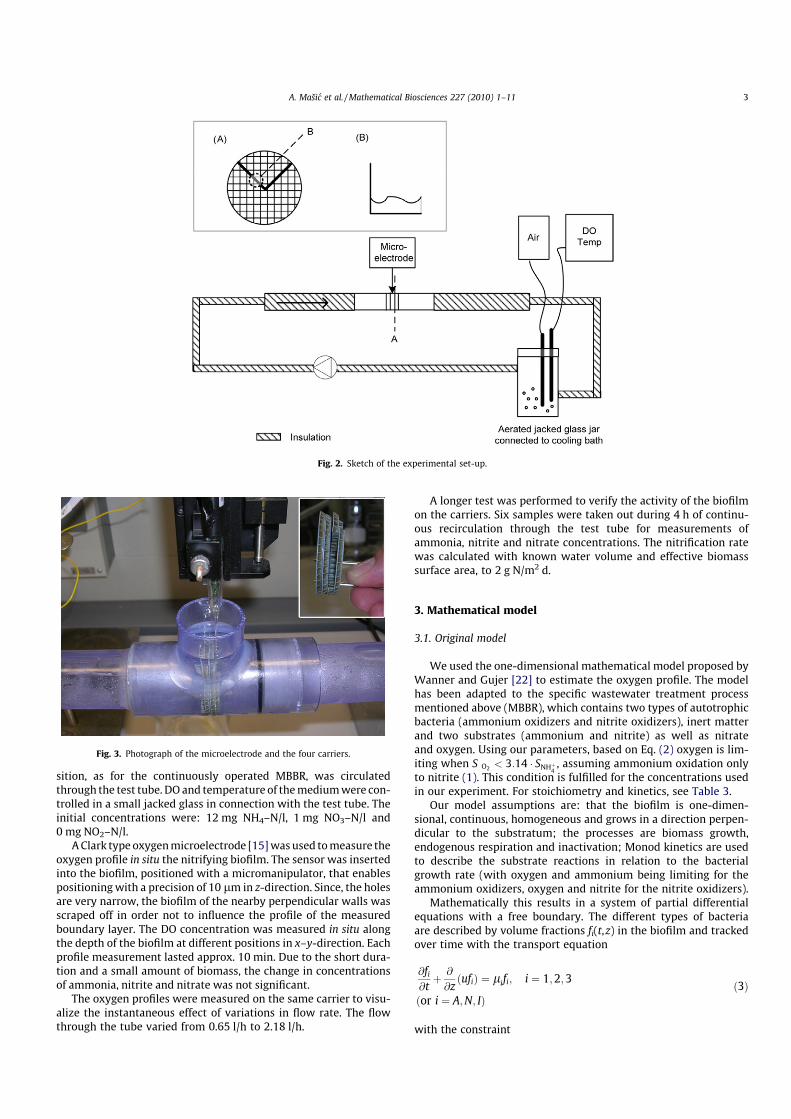
sition, as for the continuously operated MBBR, was circulatedthrough the test tube. DO and temperature of the medium were con-trolled in a small jacked glass in connection with the test tube. Theinitial concentrations were: 12 mg NH4–N/l, 1 mg NO3–N/l and0 mg NO2–N/l.
A Clark type oxygen microelectrode [15] was used to measure theoxygen profile in situ the nitrifying biofilm. The sensor was insertedinto the biofilm, positioned with a micromanipulator, that enablespositioning with a precision of 10 lm in z-direction. Since, the holesare very narrow, the biofilm of the nearby perpendicular walls wasscraped off in order not to influence the profile of the measuredboundary layer. The DO concentration was measured in situ alongthe depth of the biofilm at different positions in x–y-direction. Eachprofile measurement lasted approx. 10 min. Due to the short dura-tion and a small amount of biomass, the change in concentrationsof ammonia, nitrite and nitrate was not significant.
The oxygen profiles were measured on the same carrier to visu-alize the instantaneous effect of variations in flow rate. The flowthrough the tube varied from 0.65 l/h to 2.18 l/h.
A longer test was performed to verify the activity of the biofilmon the carriers. Six samples were taken out during 4 h of continu-ous recirculation through the test tube for measurements ofammonia, nitrite and nitrate concentrations. The nitrification ratewas calculated with known water volume and effective biomasssurface area, to 2 g N/m2 d.
3. Mathematical model
3.1. Original model
We used the one-dimensional mathematical model proposed byWanner and Gujer [22] to estimate the oxygen profile. The modelhas been adapted to the specific wastewater treatment processmentioned above (MBBR), which contains two types of autotrophicbacteria (ammonium oxidizers and nitrite oxidizers), inert matterand two substrates (ammonium and nitrite) as well as nitrateand oxygen. Using our parameters, based on Eq. (2) oxygen is lim-iting when S O2 < 3:14 � SNHþ4
, assuming ammonium oxidation onlyto nitrite (1). This condition is fulfilled for the concentrations usedin our experiment. For stoichiometry and kinetics, see Table 3.
Our model assumptions are: that the biofilm is one-dimen-sional, continuous, homogeneous and grows in a direction perpen-dicular to the substratum; the processes are biomass growth,endogenous respiration and inactivation; Monod kinetics are usedto describe the substrate reactions in relation to the bacterialgrowth rate (with oxygen and ammonium being limiting for theammonium oxidizers, oxygen and nitrite for the nitrite oxidizers).
Mathematically this results in a system of partial differentialequations with a free boundary. The different types of bacteriaare described by volume fractions fi(t,z) in the biofilm and trackedover time with the transport equation
@fi
@tþ @
@zðufiÞ ¼ lifi; i ¼ 1;2;3
ðor i ¼ A;N; IÞð3Þ
with the constraint
Fig. 2. Sketch of the experimental set-up.
Fig. 3. Photograph of the microelectrode and the four carriers.
A. Mašic et al. / Mathematical Biosciences 227 (2010) 1–11 3

X3
i¼1
fiðt; zÞ ¼ 1;
where li(t,z) denote the specific growth rates for each biomasscomponent (1/day) and u(t,z) denotes the velocity with which thebiomass moves in the biofilm (m/day). The growth rates can be cal-culated from Tables 3 and 4, for example
lA¼X6
j¼1
vAj �Pj
fA �q¼ 1
fA �q1 �lmax
A � S O2
KA;O2 þSO2
�S NHþ4
KNHþ4þSNHþ4
�fA �q�1 �bA �SO2
KA;O2 þS O2
� fA �q�1 �bA �g �SO2
KA; O2 þSO2
� fA �q�
¼lmaxA � SO2
KA;O2 þS O2
�SNHþ4
KNHþ4þSNHþ4
�ð1þgÞ �bA �SO2
KA;O2 þS O2
and u from
uðt; zÞ ¼Z z
0
X3
i¼1
fiðt; z0Þ � liðt; z0Þ !
dz0;
uðt;0Þ ¼ 0 8t P 0:
ð4Þ
The thickness of the biofilm L is described by an ordinary differen-tial equation
dLðtÞdt¼ uðt; LðtÞÞ � kLðtÞ2; ð5Þ
where k (1/m d) is the erosion parameter from [22].The substrate fields are found as the solution to a boundary va-
lue problem for four coupled diffusion–reaction equations
@Skðt; zÞ@t
¼ Dk@2Skðt; zÞ@z2 þ rkðt; zÞ;
k ¼ 1; . . . ;4
or k ¼ O2;NHþ4 ;NO�2 ;NO�3� � ð6Þ
Table 3Stoichiometric matrix.
Process j Dissolved components k Solid components i Process rate Pj
SO2 SNHþ4S NO�2 SNO�3 fA fN fI
Ammonium oxidizers (A)1. Growth � ð3:43�YAÞ
YA� 1
YA� iA
1YA
– 1 – –lmax
A � SO2KA;O2
þSO2�
S NHþ4
KNHþ4þSNHþ
4
� fA � q
2. Endogenous respiration �(1 � fXI) iA � iIfXI – – �1 – fXI bA �SO2
KA; O2þSO2� fA � q
3. Inactivation – – – – �1 – 1 bA � g �SO2
KA; O2þSO2� fA � q
Nitrite oxidizers (N)4. Growth � ð1:14�YN Þ
YN�iA � 1
YN
1YN
– 1 – lmaxN � SO2
KN;O2þS O2
�SNO�
2KNO�
2þSNO�
2
� fN � q
5. Decay/endogenous respiration �(1 � fXI) iA � iIfXI – – – �1 fXI bN �S O2
KN;O2þSO2� fN � q
6. Inactivation – – – – – �1 1 bN � g �SO2
KN;O2þSO2� fN � q
We have rkðt; zÞ ¼P6
j¼1vkjPjg
m3 �d
h iand liðt; zÞ ¼
P6j¼1
v ij Pj
fiq½1=d�.
Table 4Model parameters. (*) Adapted for 10 �C from [26].
Parameter Label Value Unit Reference
Maximum growth ratesAmmonium oxidizers lmax
A 0.3082* /day Wyffels et al. [26]Nitrite oxidizers lmax
N 0.4015* /day Wyffels et al. [26]
Monod constantsAmmonium KNHþ4
0.169 g NH4–N/m3 Own study
Nitrite KNO�2 0.302 g NO2–N/m3 Wiesmann [24]Oxygen, A KA;O2
0.5 g O2/m3 Pai [16]Oxygen, N KN;O2 0.5 g O2/m3 Pai [16]
Yield coefficientsAmmonium oxidizers YA 0.15 g COD/g NH4–N Wyffels et al. [26]Nitrite oxidizers YN 0.041 g COD/g NO2-N Wyffels et al. [26]
Reaction rate constantsDecay of ammonium oxidizers bA 0.04 /day Salem et al. [20]Decay of nitrite oxidizers bN 0.08 /day Salem et al. [20]Anoxic reduction factor for bA or bN g 0.5 – Elenter et al. [5]N content of active biomass iA 0.07 g N/g COD Picioreanu et al. [17]N content of inert biomass iI 0.02 g N/g COD Picioreanu et al. [17]Fraction of inert biomass produced by endogenous respiration fXI 0.1 g COD/g COD Picioreanu et al. [17]
Density q 10 000 g COD/m3 biofilm Picioreanu et al. [17]
Diffusion coefficients at temperature T �COxygen DO2 (682 + 29.8T � 0.0343 T2 + 0.016T3) � 10�7 m2/day Wik [25]Ammonium DNHþ4
(730 + 12.8T + 0.606 T2 � 0.00533T3) � 10�7 m2/day Wik [25]
Nitrite DNO�2 (610 + 12.8T + 0.606 T2 � 0.00533T3) � 10�7 m2/day Wik [25]Nitrate DNO�3 (610 + 12.8T + 0.606 T2 � 0.00533T3) � 10�7 m2/day Wik [25]
4 A. Mašic et al. / Mathematical Biosciences 227 (2010) 1–11
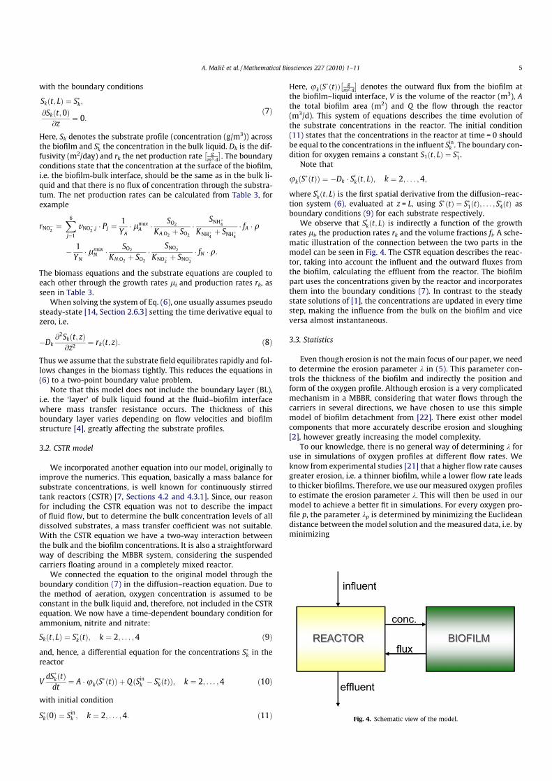
with the boundary conditions
Skðt; LÞ ¼ S�k;@Skðt;0Þ
@z¼ 0:
ð7Þ
Here, Sk denotes the substrate profile (concentration (g/m3)) acrossthe biofilm and S�k the concentration in the bulk liquid. Dk is the dif-fusivity (m2/day) and rk the net production rate g
m3 �d
� �. The boundary
conditions state that the concentration at the surface of the biofilm,i.e. the biofilm-bulk interface, should be the same as in the bulk li-quid and that there is no flux of concentration through the substra-tum. The net production rates can be calculated from Table 3, forexample
rNO�2 ¼X6
j¼1
vNO�2 ;j � Pj ¼1
YA� lmax
A � SO2
KA;O2 þ SO2
�SNHþ4
KNHþ4þ SNHþ4
� fA � q
� 1YN� lmax
N � SO2
KN;O2 þ SO2
�SNO�2
KNO�2 þ SNO�2
� fN � q:
The biomass equations and the substrate equations are coupled toeach other through the growth rates li and production rates rk, asseen in Table 3.
When solving the system of Eq. (6), one usually assumes pseudosteady-state [14, Section 2.6.3] setting the time derivative equal tozero, i.e.
�Dk@2Skðt; zÞ@z2 ¼ rkðt; zÞ: ð8Þ
Thus we assume that the substrate field equilibrates rapidly and fol-lows changes in the biomass tightly. This reduces the equations in(6) to a two-point boundary value problem.
Note that this model does not include the boundary layer (BL),i.e. the ‘layer’ of bulk liquid found at the fluid–biofilm interfacewhere mass transfer resistance occurs. The thickness of thisboundary layer varies depending on flow velocities and biofilmstructure [4], greatly affecting the substrate profiles.
3.2. CSTR model
We incorporated another equation into our model, originally toimprove the numerics. This equation, basically a mass balance forsubstrate concentrations, is well known for continuously stirredtank reactors (CSTR) [7, Sections 4.2 and 4.3.1]. Since, our reasonfor including the CSTR equation was not to describe the impactof fluid flow, but to determine the bulk concentration levels of alldissolved substrates, a mass transfer coefficient was not suitable.With the CSTR equation we have a two-way interaction betweenthe bulk and the biofilm concentrations. It is also a straightforwardway of describing the MBBR system, considering the suspendedcarriers floating around in a completely mixed reactor.
We connected the equation to the original model through theboundary condition (7) in the diffusion–reaction equation. Due tothe method of aeration, oxygen concentration is assumed to beconstant in the bulk liquid and, therefore, not included in the CSTRequation. We now have a time-dependent boundary condition forammonium, nitrite and nitrate:
Skðt; LÞ ¼ S�kðtÞ; k ¼ 2; . . . ;4 ð9Þ
and, hence, a differential equation for the concentrations S�k in thereactor
VdS�kðtÞ
dt¼ A �ukðS
�ðtÞÞ þ QðSink � S�kðtÞÞ; k ¼ 2; . . . ;4 ð10Þ
with initial condition
S�kð0Þ ¼ Sink ; k ¼ 2; . . . ;4: ð11Þ
Here, ukðS�ðtÞÞ g
m2 �d
� �denotes the outward flux from the biofilm at
the biofilm–liquid interface, V is the volume of the reactor (m3), Athe total biofilm area (m2) and Q the flow through the reactor(m3/d). This system of equations describes the time evolution ofthe substrate concentrations in the reactor. The initial condition(11) states that the concentrations in the reactor at time = 0 shouldbe equal to the concentrations in the influent Sin
k . The boundary con-dition for oxygen remains a constant S1ðt; LÞ ¼ S�1.
Note that
ukðS�ðtÞÞ ¼ �Dk � S0kðt; LÞ; k ¼ 2; . . . ;4;
where S0kðt; LÞ is the first spatial derivative from the diffusion–reac-tion system (6), evaluated at z = L, using S�ðtÞ ¼ S�1ðtÞ; . . . ; S�4ðtÞ asboundary conditions (9) for each substrate respectively.
We observe that S0kðt; LÞ is indirectly a function of the growthrates li, the production rates rk and the volume fractions fi. A sche-matic illustration of the connection between the two parts in themodel can be seen in Fig. 4. The CSTR equation describes the reac-tor, taking into account the influent and the outward fluxes fromthe biofilm, calculating the effluent from the reactor. The biofilmpart uses the concentrations given by the reactor and incorporatesthem into the boundary conditions (7). In contrast to the steadystate solutions of [1], the concentrations are updated in every timestep, making the influence from the bulk on the biofilm and viceversa almost instantaneous.
3.3. Statistics
Even though erosion is not the main focus of our paper, we needto determine the erosion parameter k in (5). This parameter con-trols the thickness of the biofilm and indirectly the position andform of the oxygen profile. Although erosion is a very complicatedmechanism in a MBBR, considering that water flows through thecarriers in several directions, we have chosen to use this simplemodel of biofilm detachment from [22]. There exist other modelcomponents that more accurately describe erosion and sloughing[2], however greatly increasing the model complexity.
To our knowledge, there is no general way of determining k foruse in simulations of oxygen profiles at different flow rates. Weknow from experimental studies [21] that a higher flow rate causesgreater erosion, i.e. a thinner biofilm, while a lower flow rate leadsto thicker biofilms. Therefore, we use our measured oxygen profilesto estimate the erosion parameter k. This will then be used in ourmodel to achieve a better fit in simulations. For every oxygen pro-file p, the parameter kp is determined by minimizing the Euclideandistance between the model solution and the measured data, i.e. byminimizing
Fig. 4. Schematic view of the model.
A. Mašic et al. / Mathematical Biosciences 227 (2010) 1–11 5

EpðkpÞ ¼XMp
i¼1
d2p;iðkpÞ; ð12Þ
where Mp is the number of data points of the oxygen profile. For thepth oxygen profile the distance dp,i is computed as
d2p;iðkpÞ ¼ min
jðzp;iðkpÞ � zp;jÞ2 þ ðyp;iðkpÞ � yp;jÞ
2� �
; ð13Þ
where (zp,j,yp,j) are measured and ðzp;iðkpÞ; yp;iðkpÞÞ are modeledpoints on the curves. Since the scales in z- and y-direction are differ-ent (ca 4 orders of magnitude), we will standardize the axes bydividing with the length of the interval in z and y, respectively.
Due to our choice of the minimization function as the Euclideandistance, we cannot use the coefficient of determination R2 to as-sess the goodness of fit. Instead, we will use the sums of squareddistances to evaluate our model, i.e.
sp ¼X
i
d2p;i;
where a smaller sp indicates a better fit.
3.4. Numerics
For our analysis we require the steady state of the dynamic bio-film model equations (3), (5) and (10). We computed this itera-tively by time-stepping to equilibrium. In every time-stepconducted, the dissolved substrate concentrations were computedby solving the two-point boundary value problem (8), see Fig. 5.
We used Matlab to solve all our equations, following thescheme in Fig. 5. The diffusion–reaction system of equations (8)was converted to a first-order system of ordinary differential equa-tions (assuming steady-state in (6)) and was solved using a built-insolver bvp4c. By vectorizing the input to the solver (and the sys-tem of equations) one can significantly reduce computing time.The transport Eq. (3), as well as the biofilm thickness Eq. (5) andthe CSTR Eq. (10), were solved with our own finite differenceimplementation. We used lsqnonlin from the Optimization Tool-box, a built-in solver of nonlinear least squares problems, to findthe optimal k that minimizes the functional (12).
We started with an initial biofilm thickness of 50 lm with anequidistant grid and an equal distribution of ammonium and ni-trite oxidizers. The initial value for the fraction of inert biomasswas set to zero. As can be seen in the experimental set-up inFig. 3, the overall biofilm area equaled the area of three carriers.
The system of equations was then iterated with time steps ofDt = 0.1 days, until tend = 60 days. We chose 60 days to make surethat the biofilm thickness had reached steady-state.
4. Results
For the comparison between the mathematical model and theexperiments, we have 13 oxygen concentration profiles, mea-sured at five different flow rates, ranging from 0.65 l/h to2.18 l/h. Four representatives are plotted in Fig. 6. With increas-
ing flow rate, a shift of the slope of the oxygen profile to the leftoccurred, as previously observed in [11]. This indicates that, de-spite increased oxygen supply as a consequence of increasedbulk flow, the biofilm becomes thinner, the faster the bulk flowis. Hence, the increasing flow rate must have a stronger effect onbiofilm erosion, than on biofilm growth. Unfortunately, the mod-el parameter describing biofilm erosion is not a priori known.Therefore, the comparison of the mathematical model with theexperimental data was conducted in two steps. (i) In the firststep, we determined the biofilm erosion parameter k, for whichno reliable estimates can be found in the literature, from theexperimentally measured oxygen profiles. (ii) In the second stepwe compared the oxygen profiles computed with the mathemat-ical model against the experimental data.
The oxygen concentration profiles measured by the microelec-trodes cover three distinct phases: (a) the bulk liquid, in whichthe oxygen concentration can be assumed in good approximationto be constant, (b) the mass transfer boundary layer, in which allthe resistance to oxygen transfer outside the biofilm occurs [14],and (c) the actual biofilm, in which oxygen is reduced by the bac-teria, see also Fig. 9 from [23]. Our simple mathematical model (8)for the dissolved substrate concentrations only captures phase (c),but is not able to describe the mass transfer boundary layer well.Hence, it must be expected, that using the experimental measure-ments without further postprocessing of data introduces errorswhen comparing model predictions and measurements.
Therefore, and in order to estimate the effect that this may haveon the modeling results, both steps (i) and (ii) were carried outtwice: First we used the raw data as determined in the experi-ments. Then, we repeated steps one and two above after removingthe concentration measurements in the boundary layer and thebulk. This postprocessing of the experimental data had to be per-formed manually. Neither the biofilm/liquid interface nor the tran-sition from the boundary layer to the bulk can be clearly inferredfrom the oxygen profiles in a straightforward manner. Accordingto [23] and based on theoretical considerations, the oxygen profileshould have a point of inflection at the biofilm/liquid interface, i.e.where the biofilm ends and the boundary layer begins. This pointof inflection is a consequence of the increased diffusive resistancein the biofilm, compared to the liquid phase. However, since forsmall molecules like oxygen the difference between the diffusioncoefficient in the biofilm and in the liquid phase is not very large[3], this point of inflection cannot be expected to be very pro-nounced and is easily overshadowed by measurement uncertain-ties. Therefore, the manual detection of the concentrationboundary layer from the experimental data was to some degreesubjective. In Fig. 7 we plot the concentration boundary layerthicknesses that have been estimated manually from the oxygenconcentration profiles. While no quantitative co-relation betweenbulk flow velocity and boundary layer thickness appears to beknown in the literature, to which these data could be compared,our results confirm the expectation that higher bulk flow rates im-ply a smaller mass transfer boundary layer, i.e. a faster transport ofoxygen from the bulk into the biofilm.
Fig. 5. Numerical scheme.
6 A. Mašic et al. / Mathematical Biosciences 227 (2010) 1–11

4.1. Estimation of erosion parameter k
The erosion parameter k was estimated from the experimentaloxygen profiles using the optimization procedure outlined above.For each data set this was conducted twice, once with the concentra-tion boundary layer in the data, denoted by k, and once after it wasremoved, denoted by kBL. The results are plotted in Fig. 8. The erosionparameters obtained in both cases were rather similar, but slightlyhigher for the data after removing the boundary layer than for thedata sets with the boundary layer values. In both cases, the erosionparameter k increased as Q increased, which confirms the impactof the reactor flow rate on detachment. At the lowest flow rates of0.65 l/h the measured erosion parameters lied between 200 and
250 (md)�1. These values doubled as the flow rate was increasedto 2.18 l/h. In good approximation, the relationship between k andQ can be described as linear. The lines of best fit were obtained as
kðQÞ ¼ 179þ 124Q
for the oxygen profiles including the data in the boundary layer, and
kBLðQÞ ¼ 162þ 146Q
for the data without. The corresponding goodness of fit was deter-mined as R2 = 0.88 and R2
BL ¼ 0:89. This allows us to express the apriori unknown erosion parameter in terms of the known modelparameter Q.
Fig. 6. Oxygen profiles measured at different flow rates.
0.6 0.8 1 1.2 1.4 1.6 1.8 2 2.230
40
50
60
70
80
90
100
flow Q (l/h)
boun
dary
laye
r th
ickn
ess
(μm
)
Fig. 7. Boundary layer thickness as function of the flow Q.
A. Mašic et al. / Mathematical Biosciences 227 (2010) 1–11 7
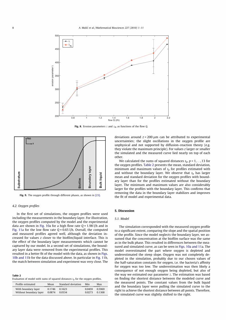
4.2. Oxygen profiles
In the first set of simulations, the oxygen profiles were usedincluding the measurements in the boundary layer. For illustration,the oxygen profiles computed by the model and the experimentaldata are shown in Fig. 10a for a high flow rate Q = 1.98 l/h and inFig. 11a for the low flow rate Q = 0.65 l/h. Overall, the computedand measured profiles agreed well, although the deviation in-creased for values z closer to the biofilm/liquid interface. This isthe effect of the boundary layer measurements which cannot becaptured by our model. In a second set of simulations, the bound-ary layer data were removed from the experimental profiles. Thisresulted in a better fit of the model with the data, as shown in Figs.10b and 11b for the data discussed above. In particular in Fig. 11b,the match between simulation and experiment was very close. The
deviations around z = 200 lm can be attributed to experimentaluncertainties; the slight oscillations in the oxygen profile areunphysical and not supported by diffusion–reaction theory (e.g.they violate the maximum principle). For values z larger or smallerthe simulated and the measured curve lied nearly on top of eachother.
We calculated the sums of squared distances sp, p = 1, . . .,13 forthe oxygen profiles. Table 2 presents the mean, standard deviation,minimum and maximum values of sp for profiles estimated withand without the boundary layer. We observe that sp has largermean and standard deviation for the oxygen profiles with bound-ary layer than for the profiles estimated without the boundarylayer. The minimum and maximum values are also considerablylarger for the profiles with the boundary layer. This confirms thatremoving the data in the boundary layer stabilizes and improvesthe fit of model and experimental data.
5. Discussion
5.1. Model
The simulation corresponded with the measured oxygen profileto a significant extent, comparing the slope and the spatial positionof the profile. Since the model neglects the boundary layer, we as-sumed that the concentration at the biofilm surface was the sameas in the bulk phase. This resulted in differences between the mea-sured and simulated curve, as can be seen in Figs. 10a and 11a. Themodel overestimated the part where oxygen is depleted andunderestimated the steep slope. Oxygen was not completely de-pleted in the simulation, probably due to our chosen values ofthe half-saturation constants for oxygen, i.e. the bacteria’s affinityfor oxygen was too low. The underestimation was then likely aconsequence of not enough oxygen being depleted, but also ofthe way we estimated our parameter k. The estimation was basedon finding the shortest distance between the modeled curve andthe measured points. The constant values from the bulk liquidand the boundary layer were pulling the simulated curve to theright to achieve the shortest distance between all points. Therefore,the simulated curve was slightly shifted to the right.
0.8 1 1.2 1.4 1.6 1.8 2 2.2200
250
300
350
400
450
500
flow Q (l/h)
eros
ion
para
met
er λ
λλ
BL
Fig. 8. Erosion parameters k and kBL as functions of the flow Q.
Fig. 9. The oxygen profile through different phases, as shown in [23].
Table 2Evaluation of model with sums of squared distances sp for the oxygen profiles.
Profile estimated Mean Standard deviation Min Max
With boundary layer 0.1746 0.1623 0.0459 0.5969Without boundary layer 0.0874 0.0334 0.0273 0.1368
8 A. Mašic et al. / Mathematical Biosciences 227 (2010) 1–11
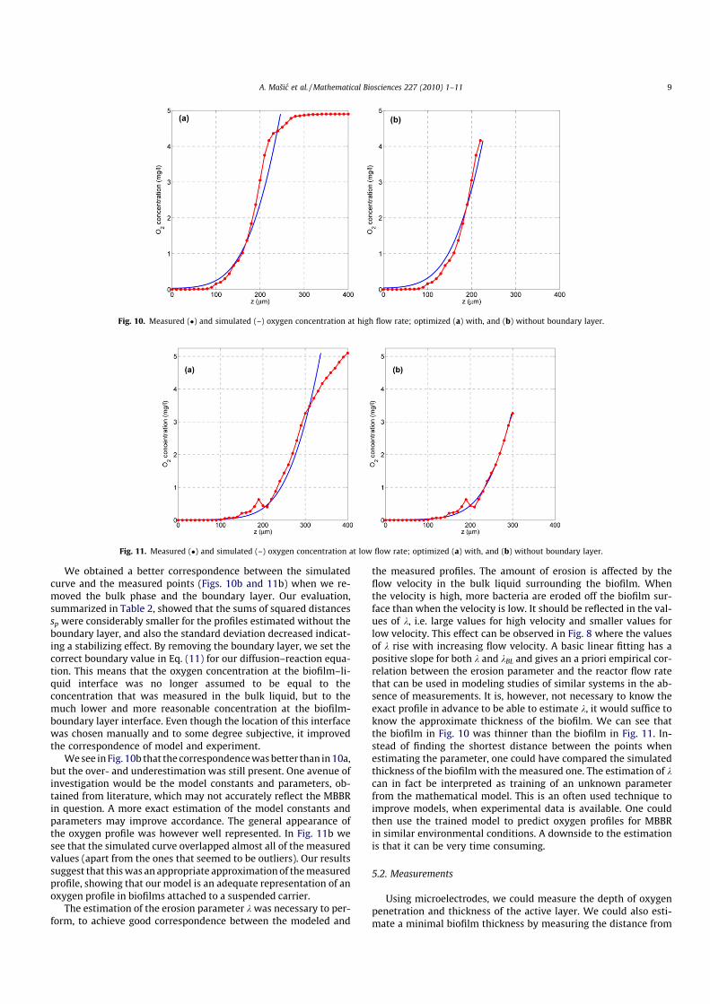
We obtained a better correspondence between the simulatedcurve and the measured points (Figs. 10b and 11b) when we re-moved the bulk phase and the boundary layer. Our evaluation,summarized in Table 2, showed that the sums of squared distancessp were considerably smaller for the profiles estimated without theboundary layer, and also the standard deviation decreased indicat-ing a stabilizing effect. By removing the boundary layer, we set thecorrect boundary value in Eq. (11) for our diffusion–reaction equa-tion. This means that the oxygen concentration at the biofilm–li-quid interface was no longer assumed to be equal to theconcentration that was measured in the bulk liquid, but to themuch lower and more reasonable concentration at the biofilm-boundary layer interface. Even though the location of this interfacewas chosen manually and to some degree subjective, it improvedthe correspondence of model and experiment.
We see in Fig. 10b that the correspondence was better than in 10a,but the over- and underestimation was still present. One avenue ofinvestigation would be the model constants and parameters, ob-tained from literature, which may not accurately reflect the MBBRin question. A more exact estimation of the model constants andparameters may improve accordance. The general appearance ofthe oxygen profile was however well represented. In Fig. 11b wesee that the simulated curve overlapped almost all of the measuredvalues (apart from the ones that seemed to be outliers). Our resultssuggest that this was an appropriate approximation of the measuredprofile, showing that our model is an adequate representation of anoxygen profile in biofilms attached to a suspended carrier.
The estimation of the erosion parameter k was necessary to per-form, to achieve good correspondence between the modeled and
the measured profiles. The amount of erosion is affected by theflow velocity in the bulk liquid surrounding the biofilm. Whenthe velocity is high, more bacteria are eroded off the biofilm sur-face than when the velocity is low. It should be reflected in the val-ues of k, i.e. large values for high velocity and smaller values forlow velocity. This effect can be observed in Fig. 8 where the valuesof k rise with increasing flow velocity. A basic linear fitting has apositive slope for both k and kBL and gives an a priori empirical cor-relation between the erosion parameter and the reactor flow ratethat can be used in modeling studies of similar systems in the ab-sence of measurements. It is, however, not necessary to know theexact profile in advance to be able to estimate k, it would suffice toknow the approximate thickness of the biofilm. We can see thatthe biofilm in Fig. 10 was thinner than the biofilm in Fig. 11. In-stead of finding the shortest distance between the points whenestimating the parameter, one could have compared the simulatedthickness of the biofilm with the measured one. The estimation of kcan in fact be interpreted as training of an unknown parameterfrom the mathematical model. This is an often used technique toimprove models, when experimental data is available. One couldthen use the trained model to predict oxygen profiles for MBBRin similar environmental conditions. A downside to the estimationis that it can be very time consuming.
5.2. Measurements
Using microelectrodes, we could measure the depth of oxygenpenetration and thickness of the active layer. We could also esti-mate a minimal biofilm thickness by measuring the distance from
Fig. 10. Measured (�) and simulated (–) oxygen concentration at high flow rate; optimized (a) with, and (b) without boundary layer.
Fig. 11. Measured (�) and simulated (–) oxygen concentration at low flow rate; optimized (a) with, and (b) without boundary layer.
A. Mašic et al. / Mathematical Biosciences 227 (2010) 1–11 9

the origin to the assumed biofilm-boundary layer interface; inFig. 10 it was approx. 220 lm and in Fig. 11 approx. 300 lm. Itwas however not possible to measure the actual thickness, sincewe did not reach substratum with the microelectrode.
It can easily be seen in the Figures that a higher flow rate gave athinner boundary layer, while a lower flow rate gave a thickerlayer. This impacted the actual oxygen concentration at the biofilmsurface. In Fig. 10a, the oxygen concentration dropped ca 0.8 mg/lover the boundary layer, but in Fig. 11a it dropped ca 1.7 mg/l. Thismeans that the true oxygen concentration at the biofilm surface inFig. 11 was lower than in Fig. 10, even if the bulk oxygen concen-trations suggested the opposite. The amount of oxygen available tothe biofilm is certainly important for the nitrification rate.
Our expectation on the effect of a higher flow was a deeper pen-etration of oxygen due to higher convection, resulting in a thickeractive layer. A short term change in flow velocity was not expectedto influence the structure of the biofilm.
However, measurements at varying flow showed that the activelayer was thinner at instantaneous higher flow. If the measure-ments were made long term on two separate systems with highversus low flow, the explanation would be more related to mor-phology. A biofilm created at higher flow rate, with thinner bound-ary layer and, therefore, higher oxygen concentration at the biofilmsurface, would have a limited biofilm thickness due to a higher ero-sion factor. It would, therefore, benefit by having a more compactmorphology, due to the presence of more active bacteria per vol-ume unit, which contradictory would have a negative effect on dif-fusion within the biofilm. At lower flow rate, with thickerboundary layer and lower oxygen concentration at the biofilm sur-face, the biofilm would then preferably have a thicker, but openand diffuse structure that maximized the surface area towardsthe bulk phase. An open biofilm structure would allow further oxy-gen diffusion until a point where extended growth had a negativeeffect, i.e. it would clog the holes in the carriers, inhibiting bothconvection and diffusion of oxygen.
These long term effects could however not explain the outcomefrom our experiment. A potential effect on the biofilm at a higher flowrate was an immediate increase of pressure, making the biofilm morecompact. Similar observations have been made by Hille et al. [11] forlow density biomass, implying our biofilm being voluminous.
Note that the microelectrode measurements have been per-formed in situ on carriers. Since measurements on moving sus-pended carriers are extremely difficult to carry out, evenimpossible with today’s techniques, we had to fixate our carriers.Even when fixated, it was challenging to reach into the depths ofa biofilm on a carrier, given the complexity of their design. Ourmeasurements on BiofilmChip P are an important step towardsacquiring a better understanding of biofilms on suspended carriers.They illustrated the morphology and function of the biofilm andexplained the importance of decreasing the boundary layer toachieve efficient utilization of oxygen.
The data gathered could be used in design of new carriers. It isalso possible to build a model specifically for MBBR, perhaps usingmore in situ measurements. It is apparent that the flow velocity haslarge impact, even when working with suspended carriers. The un-der- and overestimation by the mathematical model of the oxygenprofile at high flow rate in Fig. 10 indicated that the model does nottake into account the compression caused by increased flow rate.This should be incorporated into mathematical models, in particu-lar when studying short term effects.
To improve the oxygen utilization in process design by decreas-ing the boundary layer, it would be necessary to increase the mix-ing in the reactor either mechanically or by enhanced aeration.Thus, the potential gain is counteracted by increased energy con-sumption. The mathematical model will help us to go beyond theprocess design and instead evaluate the effect of different carrier
shapes, with the ambition of making process operation more en-ergy efficient.
6. Conclusions
Simulations and measurements of oxygen profiles in a nitrifyingbiofilm on suspended BiofilmChip P carriers were performed fordifferent flow velocities. The following conclusions were drawnfrom these experiments:
� Instead of using the inflow concentration of the MBBR reactor asthe bulk concentration value for the biofilm model, we added abalance equation in form of a CSTR equation. This allowed toaccount for the decreased concentration of ammonium, nitriteand nitrate in the suspended phase due to microbial activityin the biofilm and improved the computation of the oxygenconcentration profile. It increased the accuracy of the boundarycondition and gave a more detailed model description. Eventhough we used a simple one-dimensional mathematicalmodel, we were able to mimic the development of a biofilmin general and to calculate the concentration profiles in partic-ular. Advantages of a simpler model are easier set up and fastercalculations.� For various bulk flow rates, we carried out microelectrode mea-
surements in situ on suspended carriers, on BiofilmChip P inparticular. The measured oxygen concentration profiles wereused for comparison with and validation of the mathematicalmodel. It is however important to note that our measurementswere performed on fixated carriers, since no currently availabletechnique makes it possible to measure on moving carriers.� Using microelectrodes, it was possible to estimate the biofilm
thickness as well as the thickness of the mass transfer boundarylayer. In particular, we were able to show the dependence of thelatter two on the bulk flow rate. Our results confirm the impor-tance of decreasing the boundary layer thickness to achieve effi-cient utilization of oxygen.� Measurements of oxygen profiles with microelectrodes gave
suitable information for training of the erosion parameters kfor different flow rates. This lead to a simple empirical relation-ship between erosion parameters and bulk flow rate, which canbe used in predictive mathematical modeling of the oxygenconcentration profiles under similar conditions.
Acknowledgments
The authors thank Sami Brandt (CTS, Malmö University 2008),Mattias Hansson (CTS, Malmö University) and Roland Möhle (ibvt,TU Braunschweig 2007) for their help and many engagingdiscussions.
We would also like to thank Biofilms – Research Center for Bioin-terfaces at Malmö University, Sweden for supporting our work.
Appendix A. Medium composition
All amounts quoted as mg/l: NH4Cl 595, KH2PO4 6.0, Peptonewater 3.0, NaHCO3 2 � 103, NaOH 50, MgSO4�7H2O 0.48, CaCl2�2H2O0.58, MnCl2�4H2O 0.192, CoCl2�6H2O 0.048, NiCl2�6H2O 0.024, ZnCl2
0.026, CuSO4�5H2O 0.01, FeSO4�7H2O 0.2, BH3O3 0.52 � 10�4, Na-MoO4�2H2O 2.2 � 10�4, Na2SeO3�5H2O 1.125 � 10�4, NaWO3�2H2O1.4 � 10�4.
References
[1] E. Alpkvist, J. Bengtsson, N.C. Overgaard, M. Christensson, A. Heyden,Simulation of nitrification of municipal wastewater in a moving bed biofilm
10 A. Mašic et al. / Mathematical Biosciences 227 (2010) 1–11
process: a bottom-up approach based on a 2d-continuum model for growthand detachment, Water Science and Technology 55 (2007) 247.
[2] E. Alpkvist, I. Klapper, Description of mechanical response includingdetachment using a novel particle model of biofilm/flow interaction, WaterScience and Technology 55 (2007) 265.
[3] J. Bryers, F. Drummond, Local macromolecule diffusion coefficients instructurally non-uniform bacterial biofilms using fluorescence recovery afterphotobleaching (frap), Biotechnology and Bioengineering 60 (1998) 462.
[4] D. De Beer, P. Stoodley, Z. Lewandowski, Liquid flow and mass transport inheterogeneous biofilms, Water Research 30 (1996) 2761.
[5] D. Elenter, K. Milferstedt, W. Zhang, M. Hausner, E. Morgenroth, Influence ofdetachment on substrate removal and microbial ecology in a heterotrophic/autotrophic biofilm, Water Research 41 (2007) 4657.
[6] Y. Fu, T. Zhang, P. Bishop, Determination of effective oxygen diffusivity inbiofilms grown in a completely mixed biodrum reactor, Water Science andTechnology 29 (1994) 455.
[7] C.P.L. Grady, G.T. Daigger, H.C. Lim, Biological Wastewater Treatment:Principles and Practice, second ed., CRC Press, 1999.
[8] P. Harremoës, Criteria for nitrification in fixed film reactors, Water Science andTechnology 14 (1982) 167.
[9] L. Hem, B. Rusten, H. Ødegaard, Nitrification in a moving bed biofilm reactor,Water Research 28 (1994) 1425.
[10] M. Henze, P. Harremoës, J. La Cour Jansen, E. Arvin, Wastewater Treatment:Biological and Chemical Processes, third ed., Springer-Verlag, Berlin, 2002.
[11] A. Hille, T. Neu, D.C. Hempel, H. Horn, Oxygen profiles and biomassdistribution in biopellets of Aspergillus niger, Biotechnology andBioengineering 92 (2005) 614.
[12] H. Horn, D.C. Hempel, Growth and decay in an auto-/heterotrophic biofilm,Water Research 31 (1997) 2243.
[13] H. Horn, D.C. Hempel, Substrate utilization and mass transfer in an autotrophicbiofilm system: experimental results and numerical simulation, Biotechnologyand Bioengineering 53 (1997) 363.
[14] IWA Task Group on Biofilm Modeling, Mathematical Modeling of Biofilms. IWAScientific and Technical Report No.18, IWA Publishing, 2006.
[15] R. Lu, T. Yu, Fabrication and evaluation of an oxygen microelectrode applicableto environmental engineering and science, Journal of EnvironmentalEngineering and Science 1 (2002) 225.
[16] T.-Y. Pai, Modeling nitrite and nitrate variations in A2O process under differentreturn oxic mixed liquid using an extended model, Process Biochemistry 42(2007) 978.
[17] C. Picioreanu, J.-U. Kreft, M.C. van Loosdrecht, Particle-based multidimensionalmultispecies biofilm model, Applied and Environmental Microbiology 70(2004) 3024.
[18] W. Rauch, H. Vanhooren, P.A. Vanrolleghem, A simplified mixed-culturebiofilm model, Water Research 33 (1999) 2148.
[19] B. Rusten, H. Ødegaard, Design and operation of nutrient removal plants forvery low effluent concentrations, in: Proceedings of the Water EnvironmentFederation conference on Nutrient Removal 2007, Baltimore, Maryland, USA,March 2007, pp. 1307–1331.
[20] S. Salem, M. Moussa, M.C. van Loosdrecht, Determination of the decay rate ofnitrifying bacteria, Biotechnology and Bioengineering 94 (2006) 252.
[21] R. Santos, M. Callow, T. Bott, The structure of Pseudomonas fluorescensbiofilms in contact with flowing systems, Biofouling 4 (1991) 319.
[22] O. Wanner, W. Gujer, A multispecies biofilm model, Biotechnology andBioengineering 28 (1986) 314.
[23] S. Wäsche, H. Horn, D. Hempel, Influence of growth conditions on biofilmdevelopment and mass transfer at the bulk/biofilm interface, Water Research36 (2002) 4775.
[24] U. Wiesmann, Biological nitrogen removal from wastewater, Advances inBiochemical Engineering and Biotechnology 51 (1994) 113.
[25] T. Wik, On modeling the dynamics of fixed biofilm reactors, Ph.D. Thesis,Chalmers University of Technology, Göteborg, Sweden, 1999.
[26] S. Wyffels, S.W. van Hulle, P. Boeckx, E.I. Volcke, O. van Cleemput, P.A.Vanrolleghem, W. Verstraete, Modeling and simulation of oxygen-limitedpartial nitritation in a membrane-assisted bioreactor (MBR), Biotechnologyand Bioengineering 86 (2004) 531.
A. Mašic et al. / Mathematical Biosciences 227 (2010) 1–11 11