University of WindsorScholarship at UWindsor

Electronic Theses and Dissertations

7-11-2015

INVESTIGATING THE FEASIBILITY OFDOWNSIZING BY HAVING TWO SMALLERENGINES IN AN AUTOMOBILEShravan Kumar SadhuUniversity of Windsor

Follow this and additional works at: http://scholar.uwindsor.ca/etd

This online database contains the full-text of PhD dissertations and Masters’ theses of University of Windsor students from 1954 forward. Thesedocuments are made available for personal study and research purposes only, in accordance with the Canadian Copyright Act and the CreativeCommons license—CC BY-NC-ND (Attribution, Non-Commercial, No Derivative Works). Under this license, works must always be attributed to thecopyright holder (original author), cannot be used for any commercial purposes, and may not be altered. Any other use would require the permission ofthe copyright holder. Students may inquire about withdrawing their dissertation and/or thesis from this database. For additional inquiries, pleasecontact the repository administrator via email (scholarship@uwindsor.ca) or by telephone at 519-253-3000ext. 3208.

Recommended CitationSadhu, Shravan Kumar, "INVESTIGATING THE FEASIBILITY OF DOWNSIZING BY HAVING TWO SMALLER ENGINES INAN AUTOMOBILE" (2015). Electronic Theses and Dissertations. Paper 5296.

INVESTIGATING THE FEASIBILITY OF DOWNSIZING BY HAVING TWO

SMALLER ENGINES IN AN AUTOMOBILE

By

SHRAVAN KUMAR SADHU

A Thesis

Submitted to the Faculty of Graduate Studies

through the Department of Mechanical, Automotive & Materials Engineering

in Partial Fulfillment of the Requirements for

the Degree of Master of Applied Science

at the University of Windsor

Windsor, Ontario, Canada

2015

© 2015 SHRAVAN KUMAR SADHU

INVESTIGATING THE FEASIBILITY OF DOWNSIZING BY HAVING TWO

SMALLER ENGINES IN AN AUTOMOBILE

by

SHRAVAN KUMAR SADHU

APPROVED BY:

______________________________________________

S. Das

Department of Civil and Environmental Engineering

______________________________________________

G. Rankin

Department of Mechanical, Automotive & Materials Engineering

______________________________________________

L. Oriet, Advisor

Department of Mechanical, Automotive & Materials Engineering

April 2, 2015

iii | P a g e

DECLARATION OF ORIGINALITY I hereby certify that I am the sole author of this thesis and that no part of this thesis has been

published or submitted for publication.

I certify that, to the best of my knowledge, my thesis does not infringe upon anyone’s copyright

nor violate any proprietary rights and that any ideas, techniques, quotations, or any other

material from the work of other people included in my thesis, published or otherwise, are fully

acknowledged in accordance with the standard referencing practices. Furthermore, to the extent

that I have included copyrighted material that surpasses the bounds of fair dealing within the

meaning of the Canada Copyright Act, I certify that I have obtained a written permission from

the copyright owner(s) to include such material(s) in my thesis and have included copies of

such copyright clearances to my appendix.

I declare that this is a true copy of my thesis, including any final revisions, as approved by my

thesis committee and the Graduate Studies office, and that this thesis has not been submitted

for a higher degree to any other University or Institution.

iv | P a g e

ABSTRACT

In this competitive era, there is an increasing demand to address the problem of

powertrain matching in automobiles, one amongst the significant technologies out in the market

that addresses such a problem, is cylinder deactivation technology. While this technology

mitigates the part load losses in an automobile, due to its method of operation, is subjected to

frictional losses from the deactivated cylinders, which hinder the additional benefit that could

otherwise be capitalised on, to improve the fuel economy. For this reason, a new strategy is

presented through this thesis, which eliminates the above discussed frictional losses even while

addressing the part load performance of the engine.

v | P a g e

ACKNOWLEDGEMENTS

I would like to thank my supervisor, Dr Leo Oriet, for all his efforts in taking the initiative and

providing me the software required to pursue my thesis work. I would also like to thank Dave

McKenzie for his time and efforts in comparing the available software and aiding me to pick

the right software that suited my research pursuits.

I would like to express my sincere gratitude to AVL for providing me a free license of the AVL

CRUISE and BOOST software, without their support this project would not have been possible.

I would like to acknowledge that most of the data, used for building the models in this project,

has been used from the examples and the user guide of AVL software.

A special thanks to Mark Gryn for his continuous support in maintaining the software’s license.

I would also like to thank my MASc thesis committee, Dr. G Rankin and Dr. S Das for their

valuable time and suggestions.

I am grateful to all my friends and family members for their support in making this project

successful.

vi | P a g e

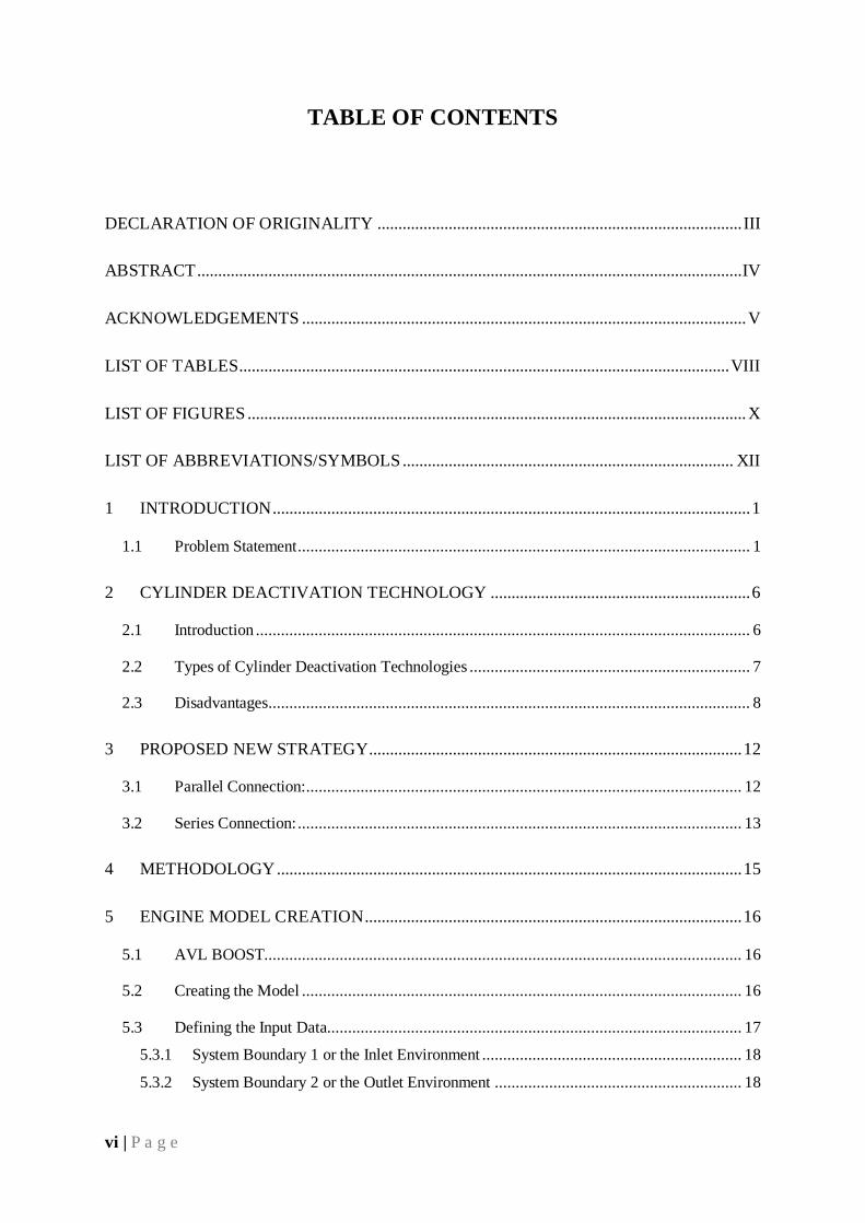
TABLE OF CONTENTS

DECLARATION OF ORIGINALITY ....................................................................................... III

ABSTRACT .................................................................................................................................. IV

ACKNOWLEDGEMENTS .......................................................................................................... V

LIST OF TABLES..................................................................................................................... VIII

LIST OF FIGURES ....................................................................................................................... X

LIST OF ABBREVIATIONS/SYMBOLS ............................................................................... XII

1 INTRODUCTION .................................................................................................................. 1

1.1 Problem Statement ............................................................................................................ 1

2 CYLINDER DEACTIVATION TECHNOLOGY .............................................................. 6

2.1 Introduction ...................................................................................................................... 6

2.2 Types of Cylinder Deactivation Technologies ................................................................... 7

2.3 Disadvantages ................................................................................................................... 8

3 PROPOSED NEW STRATEGY......................................................................................... 12

3.1 Parallel Connection: ........................................................................................................ 12

3.2 Series Connection: .......................................................................................................... 13

4 METHODOLOGY ............................................................................................................... 15

5 ENGINE MODEL CREATION .......................................................................................... 16

5.1 AVL BOOST.................................................................................................................. 16

5.2 Creating the Model ......................................................................................................... 16

5.3 Defining the Input Data................................................................................................... 17

5.3.1 System Boundary 1 or the Inlet Environment .............................................................. 18

5.3.2 System Boundary 2 or the Outlet Environment ........................................................... 18

vii | P a g e

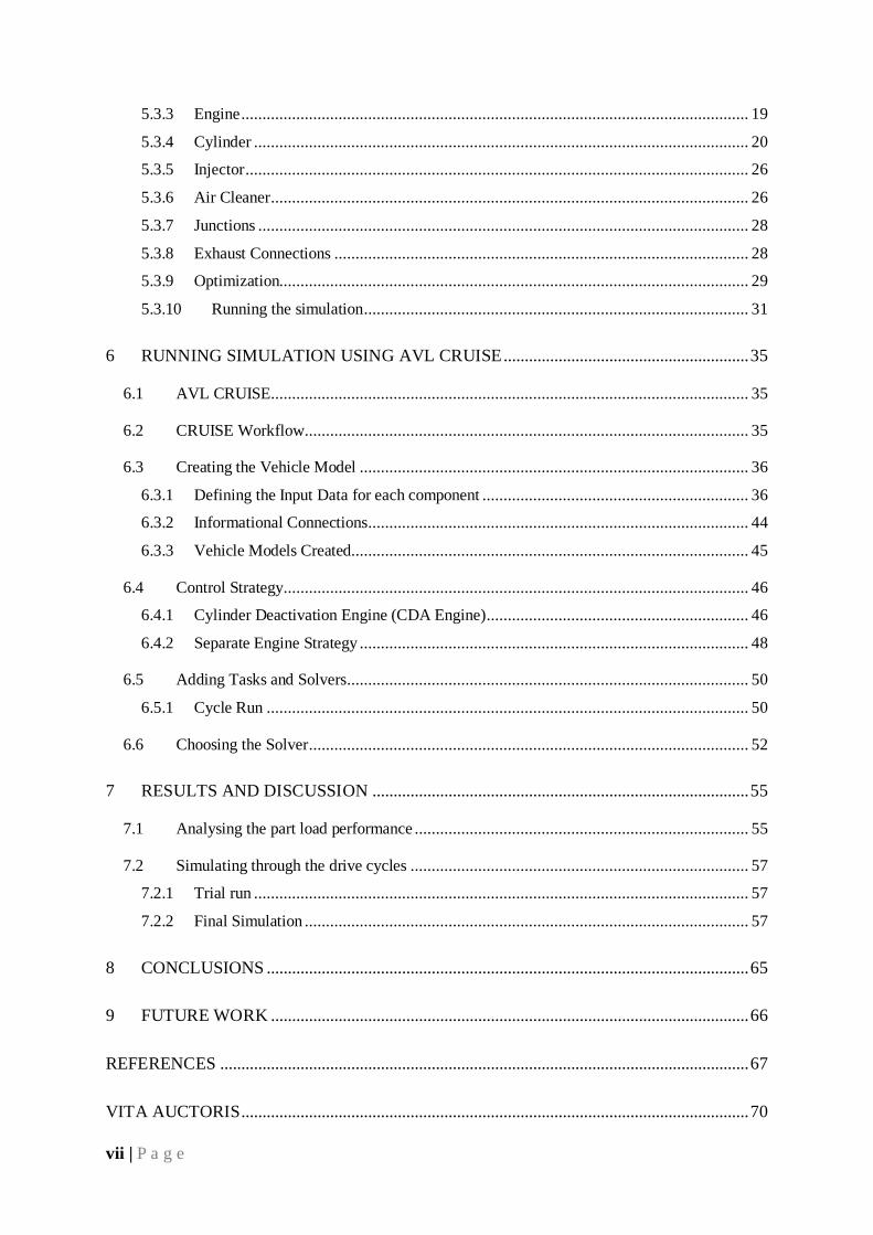
5.3.3 Engine ........................................................................................................................ 19

5.3.4 Cylinder ..................................................................................................................... 20

5.3.5 Injector ....................................................................................................................... 26

5.3.6 Air Cleaner ................................................................................................................. 26

5.3.7 Junctions .................................................................................................................... 28

5.3.8 Exhaust Connections .................................................................................................. 28

5.3.9 Optimization............................................................................................................... 29

5.3.10 Running the simulation ........................................................................................... 31

6 RUNNING SIMULATION USING AVL CRUISE .......................................................... 35

6.1 AVL CRUISE................................................................................................................. 35

6.2 CRUISE Workflow ......................................................................................................... 35

6.3 Creating the Vehicle Model ............................................................................................ 36

6.3.1 Defining the Input Data for each component ............................................................... 36

6.3.2 Informational Connections .......................................................................................... 44

6.3.3 Vehicle Models Created.............................................................................................. 45

6.4 Control Strategy.............................................................................................................. 46

6.4.1 Cylinder Deactivation Engine (CDA Engine) .............................................................. 46

6.4.2 Separate Engine Strategy ............................................................................................ 48

6.5 Adding Tasks and Solvers ............................................................................................... 50

6.5.1 Cycle Run .................................................................................................................. 50

6.6 Choosing the Solver ........................................................................................................ 52

7 RESULTS AND DISCUSSION ......................................................................................... 55

7.1 Analysing the part load performance ............................................................................... 55

7.2 Simulating through the drive cycles ................................................................................ 57

7.2.1 Trial run ..................................................................................................................... 57

7.2.2 Final Simulation ......................................................................................................... 57

8 CONCLUSIONS .................................................................................................................. 65

9 FUTURE WORK ................................................................................................................. 66

REFERENCES ............................................................................................................................. 67

VITA AUCTORIS ........................................................................................................................ 70

viii | P a g e

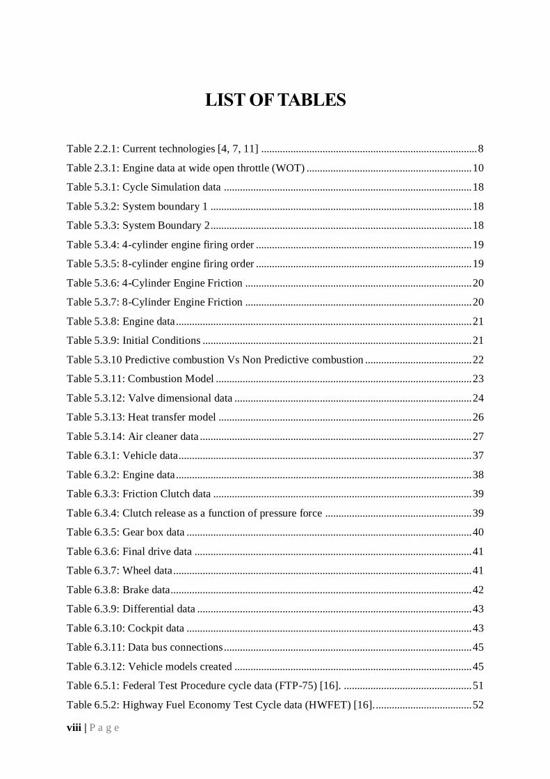
LIST OF TABLES

Table 2.2.1: Current technologies [4, 7, 11] ................................................................................. 8

Table 2.3.1: Engine data at wide open throttle (WOT) .............................................................. 10

Table 5.3.1: Cycle Simulation data ............................................................................................. 18

Table 5.3.2: System boundary 1 .................................................................................................. 18

Table 5.3.3: System Boundary 2 .................................................................................................. 18

Table 5.3.4: 4-cylinder engine firing order ................................................................................. 19

Table 5.3.5: 8-cylinder engine firing order ................................................................................. 19

Table 5.3.6: 4-Cylinder Engine Friction ..................................................................................... 20

Table 5.3.7: 8-Cylinder Engine Friction ..................................................................................... 20

Table 5.3.8: Engine data ............................................................................................................... 21

Table 5.3.9: Initial Conditions ..................................................................................................... 21

Table 5.3.10 Predictive combustion Vs Non Predictive combustion ........................................ 22

Table 5.3.11: Combustion Model ................................................................................................ 23

Table 5.3.12: Valve dimensional data ......................................................................................... 24

Table 5.3.13: Heat transfer model ............................................................................................... 26

Table 5.3.14: Air cleaner data ...................................................................................................... 27

Table 6.3.1: Vehicle data.............................................................................................................. 37

Table 6.3.2: Engine data ............................................................................................................... 38

Table 6.3.3: Friction Clutch data ................................................................................................. 39

Table 6.3.4: Clutch release as a function of pressure force ....................................................... 39

Table 6.3.5: Gear box data ........................................................................................................... 40

Table 6.3.6: Final drive data ........................................................................................................ 41

Table 6.3.7: Wheel data ................................................................................................................ 41

Table 6.3.8: Brake data................................................................................................................. 42

Table 6.3.9: Differential data ....................................................................................................... 43

Table 6.3.10: Cockpit data ........................................................................................................... 43

Table 6.3.11: Data bus connections ............................................................................................. 45

Table 6.3.12: Vehicle models created ......................................................................................... 45

Table 6.5.1: Federal Test Procedure cycle data (FTP-75) [16]. ................................................ 51

Table 6.5.2: Highway Fuel Economy Test Cycle data (HWFET) [16]. .................................... 52

ix | P a g e

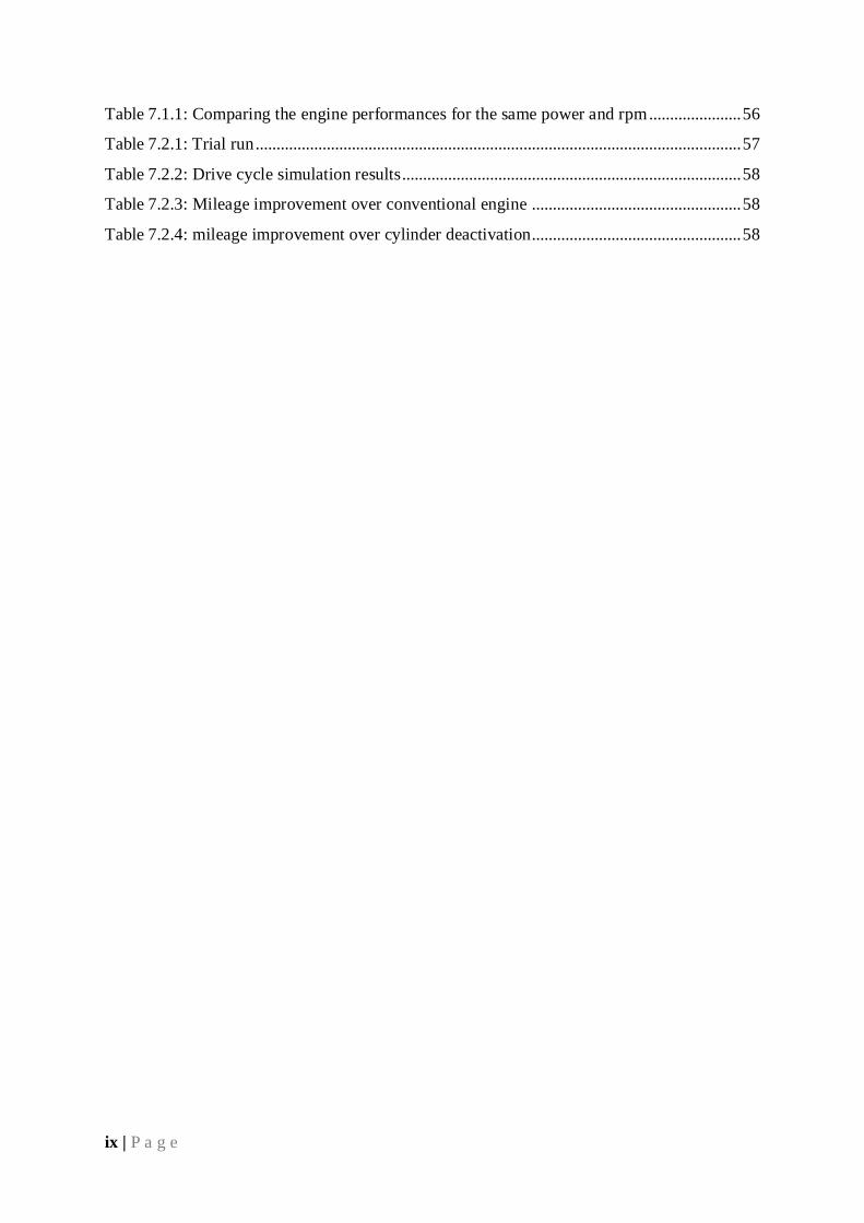
Table 7.1.1: Comparing the engine performances for the same power and rpm ...................... 56

Table 7.2.1: Trial run .................................................................................................................... 57

Table 7.2.2: Drive cycle simulation results ................................................................................. 58

Table 7.2.3: Mileage improvement over conventional engine .................................................. 58

Table 7.2.4: mileage improvement over cylinder deactivation.................................................. 58

x | P a g e

LIST OF FIGURES

Figure 1.1.1: Car Specifications [9]............................................................................................... 1

Figure 1.1.2: Driving time distribution [17] ................................................................................. 2

Figure 1.1.3: Effect of Road load on engine performance [8] ..................................................... 3

Figure 1.1.4: Engine pumping losses [10] .................................................................................... 4

Figure 1.1.5: Variation in specific fuel consumption [8] ............................................................. 5

Figure 2.2.1: Types of deactivating mechanisms [4] ................................................................... 7

Figure 2.3.1: Frictional losses in an engine [7]............................................................................. 9

Figure 3.1.1: Planetary gear system layout [12] ......................................................................... 13

Figure 3.2.1: Friction clutch components [24]............................................................................ 13

Figure 3.2.2: Separate engine strategy ........................................................................................ 14

Figure 5.2.1: 4-cylinder engine model ........................................................................................ 17

Figure 5.3.1: Crank Angle related to Combustion Duration [14] .............................................. 23

Figure 5.3.2: Valve lift curve [14] ............................................................................................... 24

Figure 5.3.3: Steady State Air Cleaner Performance ................................................................. 27

Figure 5.3.4: Flow coefficients of a junction .............................................................................. 28

Figure 5.3.5: Exhaust Connections .............................................................................................. 29

Figure 5.3.6: Plenum for a 4-cyliner engine model .................................................................... 30

Figure 5.3.7: Plenum for an 8-cylinder engine model ................................................................ 30

Figure 5.3.8: 4-Cylinder Engine Brake Torque .......................................................................... 31

Figure 5.3.9: 4-Cylinder Engine Fuel Consumption Map.......................................................... 31

Figure 5.3.10: 8-Cylinder Engine Brake Torque ........................................................................ 32

Figure 5.3.11: 8-Cylinder Engine Fuel Map ............................................................................... 32

Figure 5.3.12: CDA Engine Brake Torque ................................................................................. 33

Figure 5.3.13: CDA Engine Fuel Map ........................................................................................ 34

Figure 6.3.1: Acceleration pedal travel (%) vs load signal (%) ................................................. 44

Figure 6.3.2: 8-Cylinder conventional engine model ................................................................. 46

Figure 6.4.1: 8-cylinder CDA engine model............................................................................... 47

Figure 6.4.2: Separate Engine Strategy ....................................................................................... 50

Figure 6.5.1: Federal Test Procedure cycle velocity profile (FTP-75) ..................................... 51

Figure 6.5.2: Highway Fuel Economy Test Cycle velocity profile (HWFET) ......................... 52

xi | P a g e

Figure 7.2.1: Driving Time Distribution for conventional 8-Cylinder Engine in highway cycle

............................................................................................................................................... 59

Figure 7.2.2: Driving Time Abundance for conventional 8-Cylinder Engine in highway cycle

............................................................................................................................................... 59

Figure 7.2.3: Driving time distribution for Cylinder Deactivation Engine in highway cycle . 60

Figure 7.2.4: Driving time abundance for Cylinder Deactivation Engine in highway cycle ... 60

Figure 7.2.5: Driving time distribution for Separate Engine Strategy in highway cycle ......... 61

Figure 7.2.6: Driving Time Abundance for Separate Engine Strategy in highway cycle ........ 61

Figure 7.2.7: CDA Engine fuel flow ........................................................................................... 63

Figure 7.2.8: Separate Engine fuel flow ...................................................................................... 63

Figure 7.2.9: Fuel benefit from separate engine operation ........................................................ 64

xii | P a g e

LIST OF ABBREVIATIONS/SYMBOLS

A/f Ratio Air Fuel ratio

BMEF Brake Mean Effective Pressure

BSFC Brake Specific Fuel consumption

CCE Cylinder Cut-out

CDA Cylinder Deactivation

degC degrees centigrade

EPA Environmental Protection Agency

FTP Federal test procedure

HWFET Highway Fuel Economy Test

ISFC Indicated Specific Fuel Consumption

MPG Miles per gallon

PV Pressure Volume

RPM Revolutions per minute

VE Volumetric Efficiency

WOT Wide open throttle

VTDC Volume at Top Dead Centre

VBDC Volume at Bottom Dead Centre

1 | P a g e

1 Introduction

Globally, demand for automobiles with higher power, lower fuel consumption and lesser

emission is on the rise. Automobile manufacturers, to stay current and to improve their product

appeal, have been trying to enhance the running performance of a vehicle but are finding it

difficult to cope up with the current fuel economy standards that are getting more stringent day

by day. One of the most promising areas for increasing the fuel economy of automobiles lies

in the area of decreasing the brake specific fuel consumption.

Brake specific fuel consumption, is the amount of fuel consumed per unit power produced in a

vehicle, it gives a basic understanding of how efficiently the fuel is being utilized by the engine

to produce power.

Ever since the automobile was introduced, a major challenge the engine designers have been

trying to address is to decrease the brake specific fuel consumption in all operating conditions

in an automobile.

The nature of the driving cycle plays a vital role in utilizing the brake specific consumption to

its potential. Contemporarily, most people experience drive cycles that do not even set out to

utilise the present-day engines at anything even close to their brake specific fuel consumption

potential. This can be explained in detail by the problem statement below:

1.1 Problem Statement

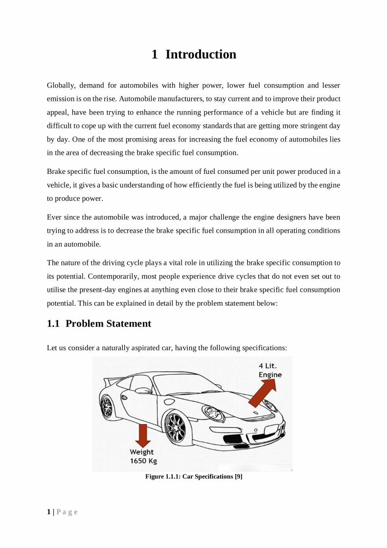
Let us consider a naturally aspirated car, having the following specifications:

Figure 1.1.1: Car Specifications [9]

2 | P a g e

Fuel Consumption City: 20 MPG

Fuel Consumption Highway: 28 MPG

Average City/Highway Fuel Consumption: 24 MPG

Corresponding Average BSFC: 0.400 g/W-hr

Optimum BSFC: 0.280 g/W-hr

When the car travels through city and highway conditions, the average fuel consumption is

about 24 MPG, this corresponds to an average brake specific fuel consumption of about 0.400

g/W-hr but the average brake specific fuel consumption for this vehicle is around 0.280 g/W-

hr [8].

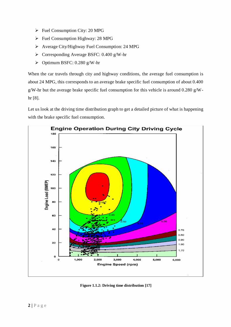
Let us look at the driving time distribution graph to get a detailed picture of what is happening

with the brake specific fuel consumption.

Figure 1.1.2: Driving time distribution [17]

3 | P a g e

It is clearly understood from the driving time distribution map that the typical road load values

are nowhere close to utilizing the optimum brake specific fuel consumption of this car.

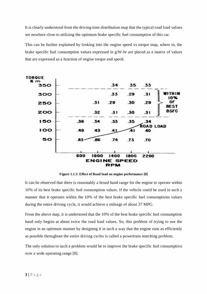
This can be further explained by looking into the engine speed vs torque map, where in, the

brake specific fuel consumption values expressed in g/W-hr are placed as a matrix of values

that are expressed as a function of engine torque and speed.

Figure 1.1.3: Effect of Road load on engine performance [8]

It can be observed that there is reasonably a broad band range for the engine to operate within

10% of its best brake specific fuel consumption values. If the vehicle could be used in such a

manner that it operates within the 10% of the best brake specific fuel consumptions values

during the entire driving cycle, it would achieve a mileage of about 37 MPG.

From the above map, it is understood that the 10% of the best brake specific fuel consumption

band only begins at about twice the road load values. So, this problem of trying to use the

engine in an optimum manner by designing it in such a way that the engine runs as efficiently

as possible throughout the entire driving cycles is called a powertrain matching problem.

The only solution to such a problem would be to improve the brake specific fuel consumption

over a wide operating range [8].

4 | P a g e

Let us try to understand the factors that hamper the brake specific fuel consumption over wide

operating ranges.

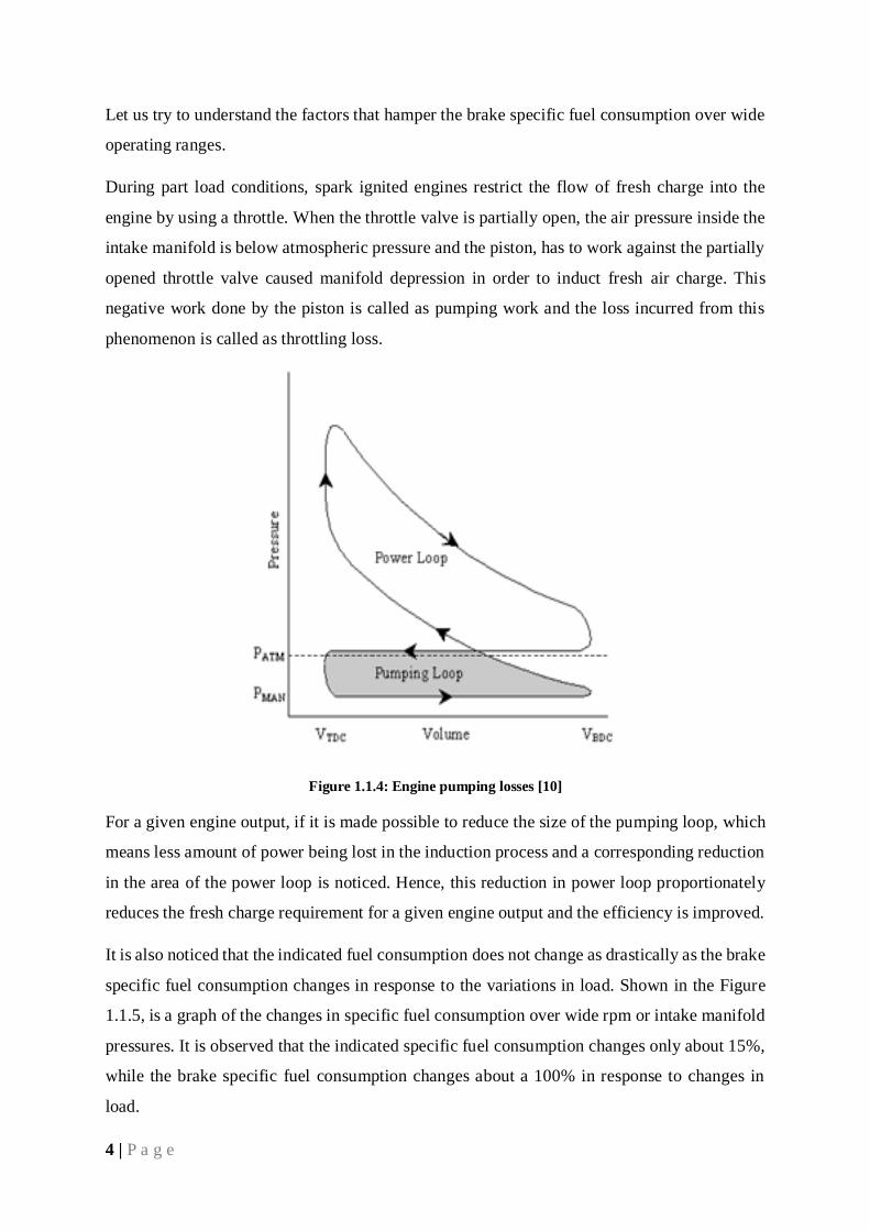
During part load conditions, spark ignited engines restrict the flow of fresh charge into the

engine by using a throttle. When the throttle valve is partially open, the air pressure inside the

intake manifold is below atmospheric pressure and the piston, has to work against the partially

opened throttle valve caused manifold depression in order to induct fresh air charge. This

negative work done by the piston is called as pumping work and the loss incurred from this

phenomenon is called as throttling loss.

Figure 1.1.4: Engine pumping losses [10]

For a given engine output, if it is made possible to reduce the size of the pumping loop, which

means less amount of power being lost in the induction process and a corresponding reduction

in the area of the power loop is noticed. Hence, this reduction in power loop proportionately

reduces the fresh charge requirement for a given engine output and the efficiency is improved.

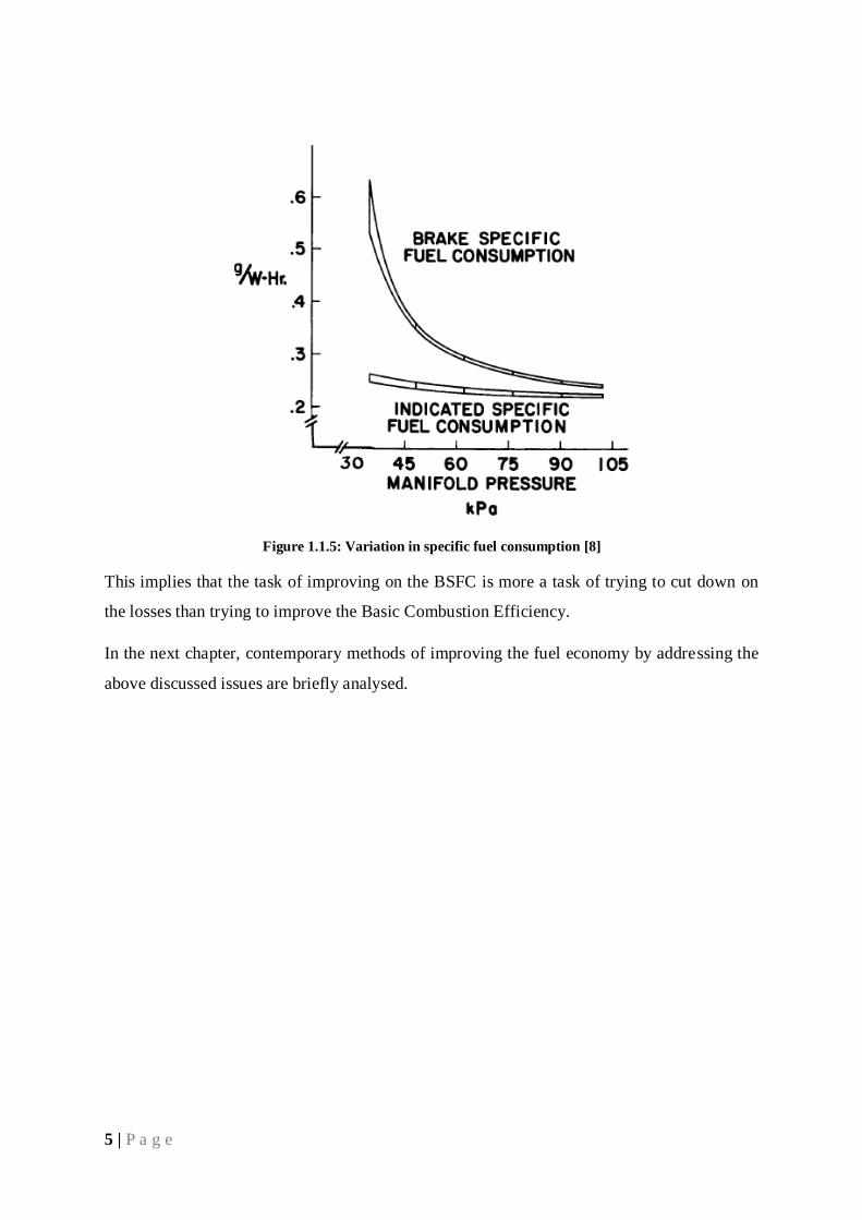
It is also noticed that the indicated fuel consumption does not change as drastically as the brake

specific fuel consumption changes in response to the variations in load. Shown in the Figure

1.1.5, is a graph of the changes in specific fuel consumption over wide rpm or intake manifold

pressures. It is observed that the indicated specific fuel consumption changes only about 15%,

while the brake specific fuel consumption changes about a 100% in response to changes in

load.

5 | P a g e

Figure 1.1.5: Variation in specific fuel consumption [8]

This implies that the task of improving on the BSFC is more a task of trying to cut down on

the losses than trying to improve the Basic Combustion Efficiency.

In the next chapter, contemporary methods of improving the fuel economy by addressing the

above discussed issues are briefly analysed.

6 | P a g e

2 Cylinder Deactivation Technology

2.1 Introduction

As discussed in the previous chapter, to eliminate the part load losses or the pumping losses in

a vehicle, for a given output, the area of the pumping loop, in the PV diagram has to be reduced.

The pumping work can be reduced by making the pressure in the intake manifold as close to

atmospheric as possible, in other words, eliminating the pressure difference that exists between

the intake manifold and outside environment leads to reduction of pumping losses in an engine.

Now to reduce this pressure difference, the throttle opening has to be increased, but the engine’s

power output is directly proportional to the throttle valve opening, so any increase in the throttle

opening to reduce the pumping loss, would lead to an increase in the power output of the

engine. Any abrupt change in the power output is not desirable to the driver. For this reason,

depending on the need, a few cylinders in the engine are sometimes turned off before the

throttle opening is increased to eliminate the part load losses. In this way the remainder of the

active cylinders need to produce more power to compensate for the power lost from the

deactivated cylinders and require the throttle valve to open wider and eliminate the pumping

losses, which is the main objective of the cylinder deactivation technology.

Cylinder Deactivation Technology, is a means of improving the fuel economy in gasoline

engines. Reduce the part load losses by varying the displacement of the engine, this is

accomplished by having a control on number of active cylinders and cutting out or deactivating

the cylinders that are not wanted during the part load operation.

Deactivation of cylinders can be done by keeping the intake and exhaust valves closed, either

before the suction stroke or after the compression stroke. When deactivated, the gasses that get

trapped in the combustion chamber are subjected to compression and expansion due to the up

and down movement of the piston during the deactivation phase, this creates an air spring inside

the combustion chamber which has virtually, no additional load on the engine.

This transition while activating and deactivating the cylinders is made seamless by making

small changes to the ignition timing, camshaft timing and also, the throttle valve opening, all

these modifications are controlled by sophisticated electronic control systems.

7 | P a g e

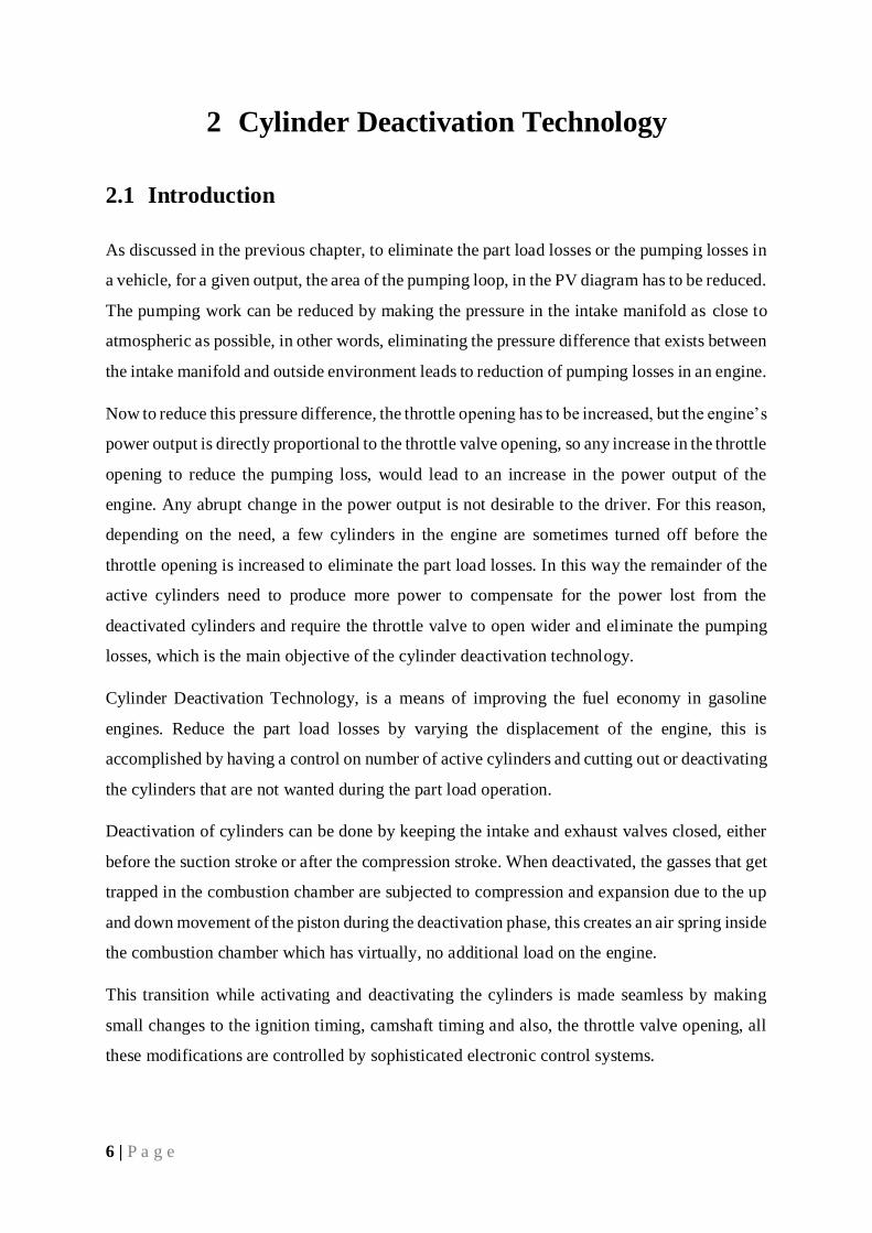
2.2 Types of Cylinder Deactivation Technologies

Cylinder deactivation technology can be classified into two kinds, depending on the type of

valve train.

Figure 2.2.1: Types of deactivating mechanisms [4]

For push road valve trains, the deactivation is initiated at the lifter by decoupling the lifter and

camshaft. A hydraulically operated pin is used to break the link between the lifter and camshaft.

For overhead valve trains, the deactivation is initiated at the rocker arm, again by the use of

solenoid controlled hydraulically operated pin to engage and break the link with the remainder

of the valve train.

It can be understood that this cylinder deactivation technology runs the cylinders at higher

volumetric efficiency zones by increasing the throttle valve opening, eliminates the part load

losses and also, at the same time reduces the valve train friction. The extent to which the valve

train friction gets reduced depends on the mechanism of valve train operation.

8 | P a g e

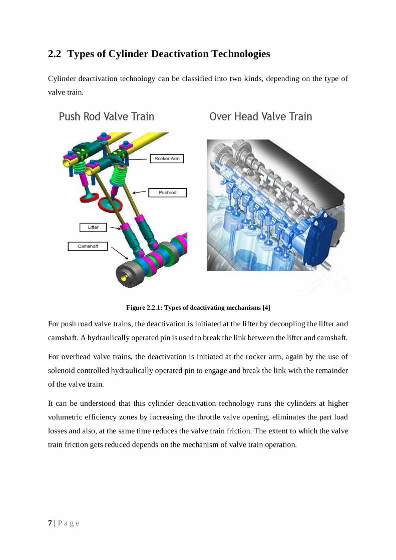
Given below are the current OEM strategies and claimed economy benefits obtained from the

use of cylinder deactivation technology.

Chrysler

Multi

Displaceme

nt (MDS)

GM

Displaceme

nt on

Demand

(DOD)

Honda

Variable

Cylinder

Management

(VCM)

Mercedes

Benz Volkswagen

Valve

Train

Push Rod

Design

Push Rod

Design

Overhead

Valve train

design

Overhead

Valve train

design

Multi Piece

cam shaft

design

Decoupling

location Lifter Lifter Rocker Arm Rocker Arm Rocker Arm

Decoupling

force Oil Pressure Oil Pressure Oil Pressure Oil Pressure

Electro

Magnetic

Actuator

Decoupling

controlled

by

Solenoid

Valve

Solenoid

Valve Solenoid Valve

Solenoid

Valve

Claimed

Benefit

City 7%

improveme

nt

Steady

CRUISE

20%

5.5% -

7.5% Fuel

economy

improveme

nt

About 7-10%

fuel economy

improvement

About 7%

fuel

economy

improvement

About 7%

fuel

economy

improvement

Table 2.2.1: Current technologies [4, 7, 11]

The United States Environmental Protection Agency (EPA) claims that on an average, the

Cylinder Deactivation Technology improves the fuel economy by 7.5%.

2.3 Disadvantages

Besides having an improvement in the fuel economy, the usage of this technology has the

following drawbacks:

The engine cools down unevenly, when the cylinders are deactivated, the exhaust gas

is entrapped in the combustion chamber, the heat generated from compression and

expansion of this exhaust gas sets in an uneven pattern in the thermal model of the

engine and also makes these deactivated cylinders cool down slowly.

9 | P a g e

A large quantity of the confined gas creates an air spring inside the combustion

chamber, leads to producing different pressures inside this chamber and would further

lead to producing greater irregularities in forces on the crankshaft.

Care should be taken to ascertain that no vacuum or suction force is produce inside the

combustion chamber, as this would cause the crankcase engine oil to be drawn into the

chamber.

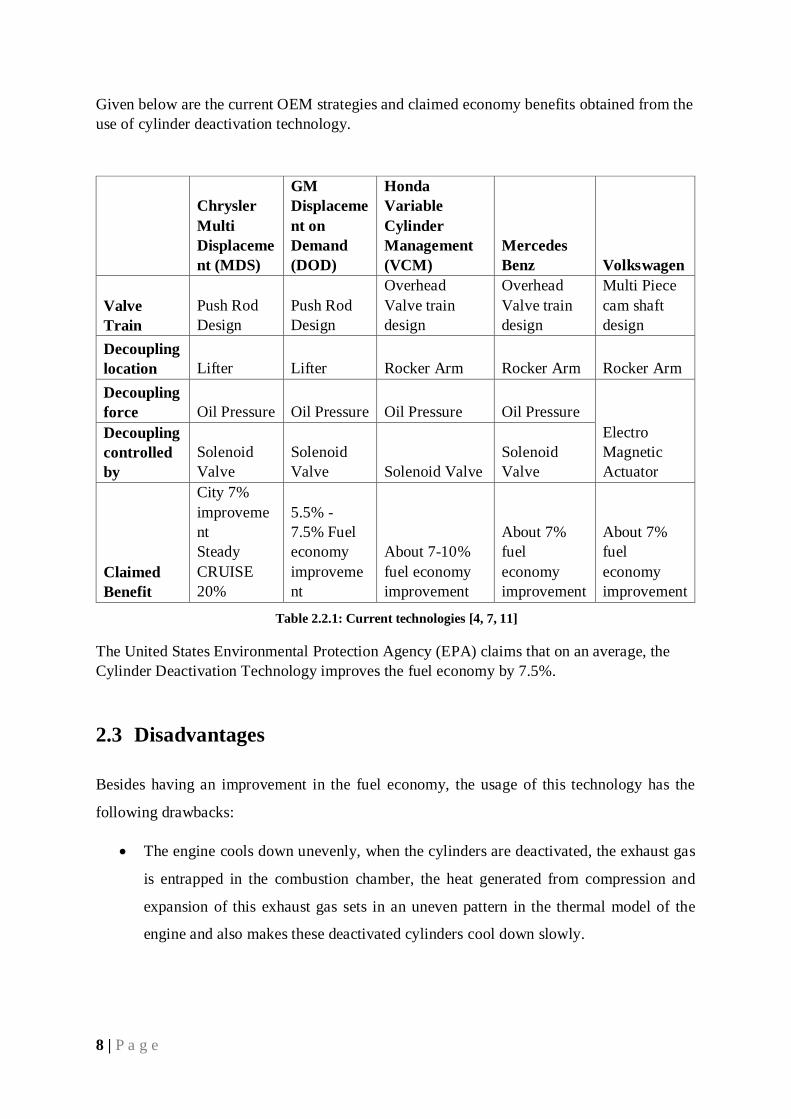
Even though the cylinders are deactivated, there is power loss incurred from the

reciprocating pistons, this loss accounts to about 65-80% of the frictional mean

effective pressure in an engine [7].

Figure 2.3.1: Frictional losses in an engine [7]

It is only this 7-15% valve train friction, shown in the above pie chart, the cylinder

deactivation technology manages to save.

A major chunk of loss is incurred through the friction from piston assembly and the

bearings, this loss in total sums up to 65-80% of the friction mean effective pressure in

an engine.

In order to analyse the variation in friction mean effective pressure over a wide range

of engine load, as depicted in Table 2.3.1, friction mean effective pressure represented

as a function of rpm and brake mean effective pressure, is taken into consideration.

10 | P a g e

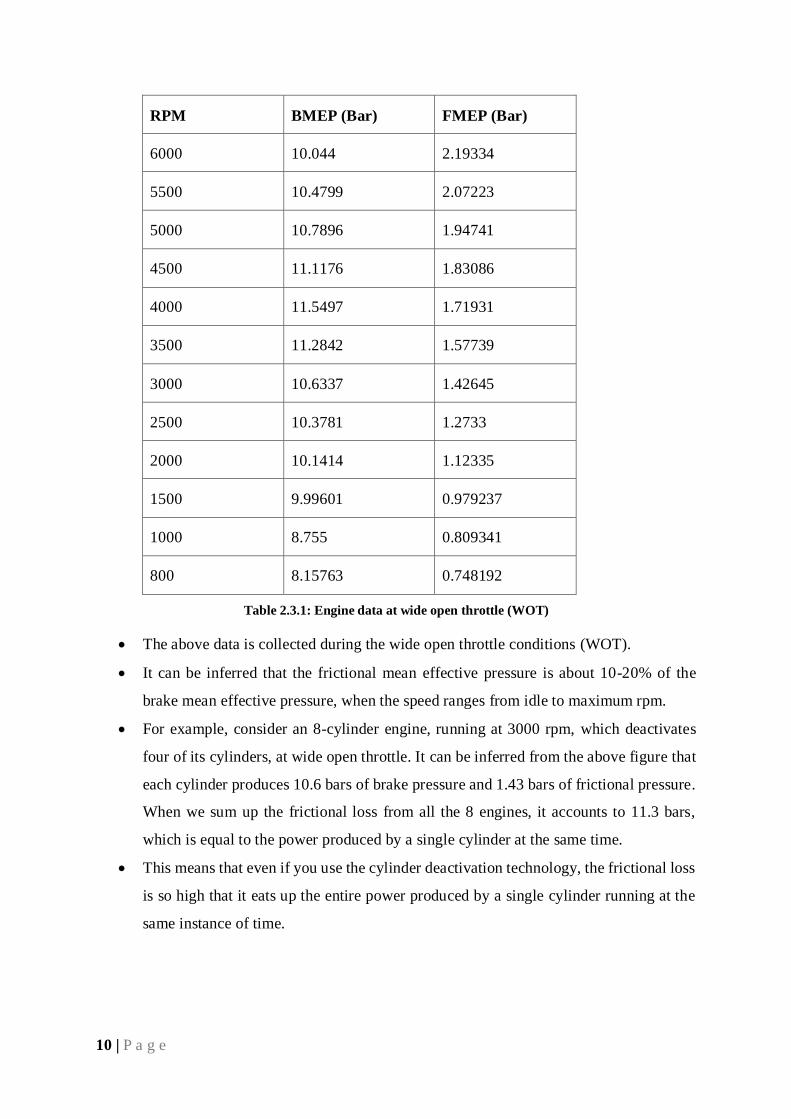
RPM BMEP (Bar) FMEP (Bar)

6000 10.044 2.19334

5500 10.4799 2.07223

5000 10.7896 1.94741

4500 11.1176 1.83086

4000 11.5497 1.71931

3500 11.2842 1.57739

3000 10.6337 1.42645

2500 10.3781 1.2733

2000 10.1414 1.12335

1500 9.99601 0.979237

1000 8.755 0.809341

800 8.15763 0.748192

Table 2.3.1: Engine data at wide open throttle (WOT)

The above data is collected during the wide open throttle conditions (WOT).

It can be inferred that the frictional mean effective pressure is about 10-20% of the

brake mean effective pressure, when the speed ranges from idle to maximum rpm.

For example, consider an 8-cylinder engine, running at 3000 rpm, which deactivates

four of its cylinders, at wide open throttle. It can be inferred from the above figure that

each cylinder produces 10.6 bars of brake pressure and 1.43 bars of frictional pressure.

When we sum up the frictional loss from all the 8 engines, it accounts to 11.3 bars,

which is equal to the power produced by a single cylinder at the same time.

This means that even if you use the cylinder deactivation technology, the frictional loss

is so high that it eats up the entire power produced by a single cylinder running at the

same instance of time.

11 | P a g e

For this reason, there is a need to curb this frictional loss while trying to improve the part load

performance to experience a maximum benefit.

In in the next chapter, a new strategy is developed to curb the frictional loss while improving

the part load performance of the engine.

12 | P a g e

3 Proposed New Strategy

For reasons explained in the previous chapter, there is an increasing need to develop a fuel

saving strategy that averts the piston motion while addressing the problem of powertrain

matching.

This is only possible if the motion of the piston is ceased while the throttle position is being

varied. For the motion to be ceased, the piston or crank shaft should possess the ability to

disengage when required.

Therefore, this requirement lead to the development of a separate engine strategy, instead of a

single large engine, two separate smaller engines would be connected to the powertrain and

one of the engines would turn off when not required. This would completely decouple the

engine from the powertrain and hence, the frictional losses are curbed while improving the part

load performance.

For example, in case a vehicle has an 8-cyliner engine that has a cubic capacity of 4 litres, it

could be replaced with two 4-cylinder engines, having a cubic capacity of 2 litres.

These separate engines can be connected in two possible ways.

3.1 Parallel Connection:

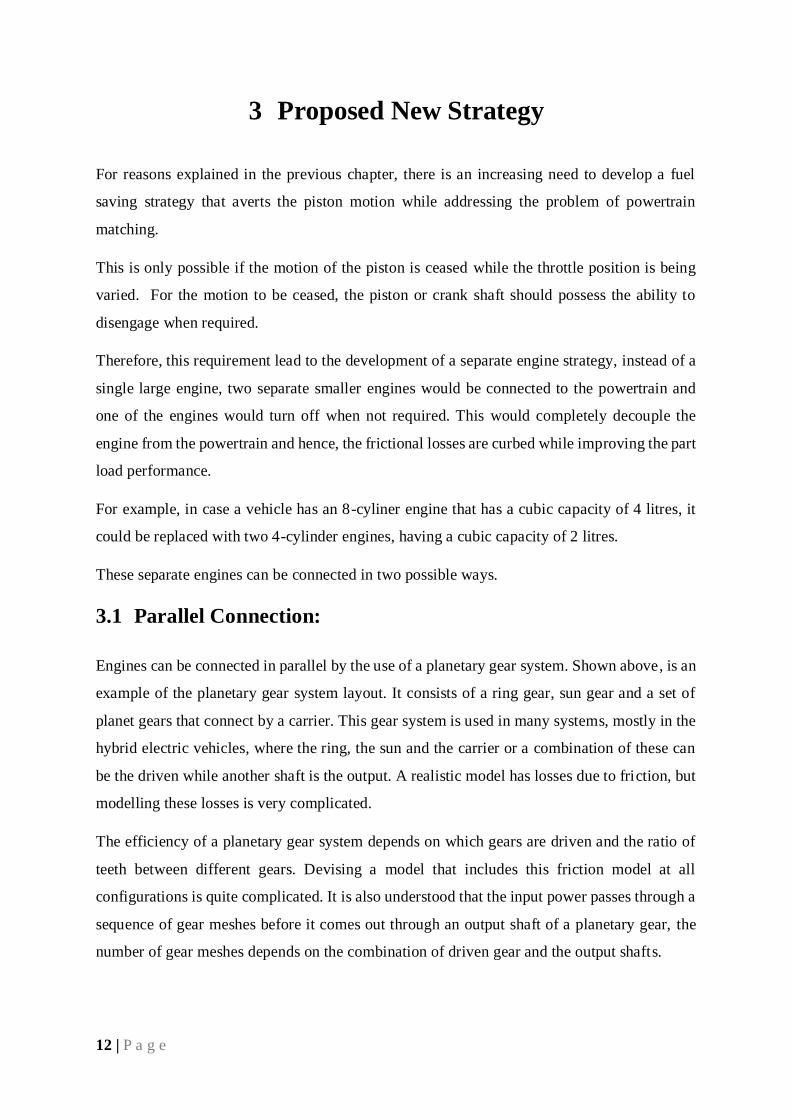
Engines can be connected in parallel by the use of a planetary gear system. Shown above, is an

example of the planetary gear system layout. It consists of a ring gear, sun gear and a set of

planet gears that connect by a carrier. This gear system is used in many systems, mostly in the

hybrid electric vehicles, where the ring, the sun and the carrier or a combination of these can

be the driven while another shaft is the output. A realistic model has losses due to friction, but

modelling these losses is very complicated.

The efficiency of a planetary gear system depends on which gears are driven and the ratio of

teeth between different gears. Devising a model that includes this friction model at all

configurations is quite complicated. It is also understood that the input power passes through a

sequence of gear meshes before it comes out through an output shaft of a planetary gear, the

number of gear meshes depends on the combination of driven gear and the output shafts.

13 | P a g e

Every gear mesh has about 2-3% loss in power, so in case we use the planetary gear, due to the

sequence of gear meshes involved in this model, the output power is only about 94-95% of the

input power, or in other words, the usage of this model causes about 5-6% loss in the power.

To avoid the above stated power loss, a method described below is chosen for connecting the

two smaller separate engines.

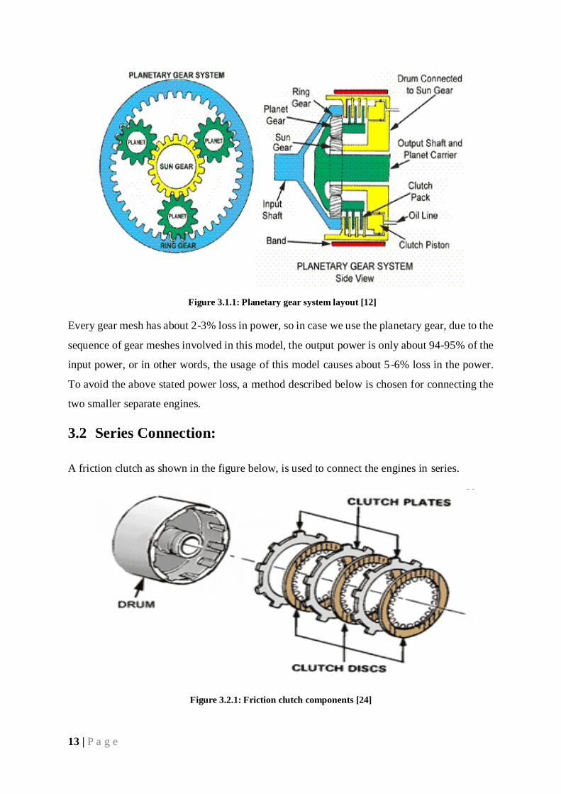
3.2 Series Connection:

A friction clutch as shown in the figure below, is used to connect the engines in series.

Figure 3.2.1: Friction clutch components [24]

Figure 3.1.1: Planetary gear system layout [12]

14 | P a g e

The clutches are connected to the flywheel of the engine, so a minor modification has to be

made to the engine that sits in the front, for this engine a flywheel has to be attached to the

crank shaft and connects on the rear side, i.e., on the side that is on the other end of the

conventional flywheel location.

The flywheel is equipped with a friction surface, and this is pressed against the friction surface

of the clutch discs, this makes the flywheel lock with the clutch and rotate as one unit.

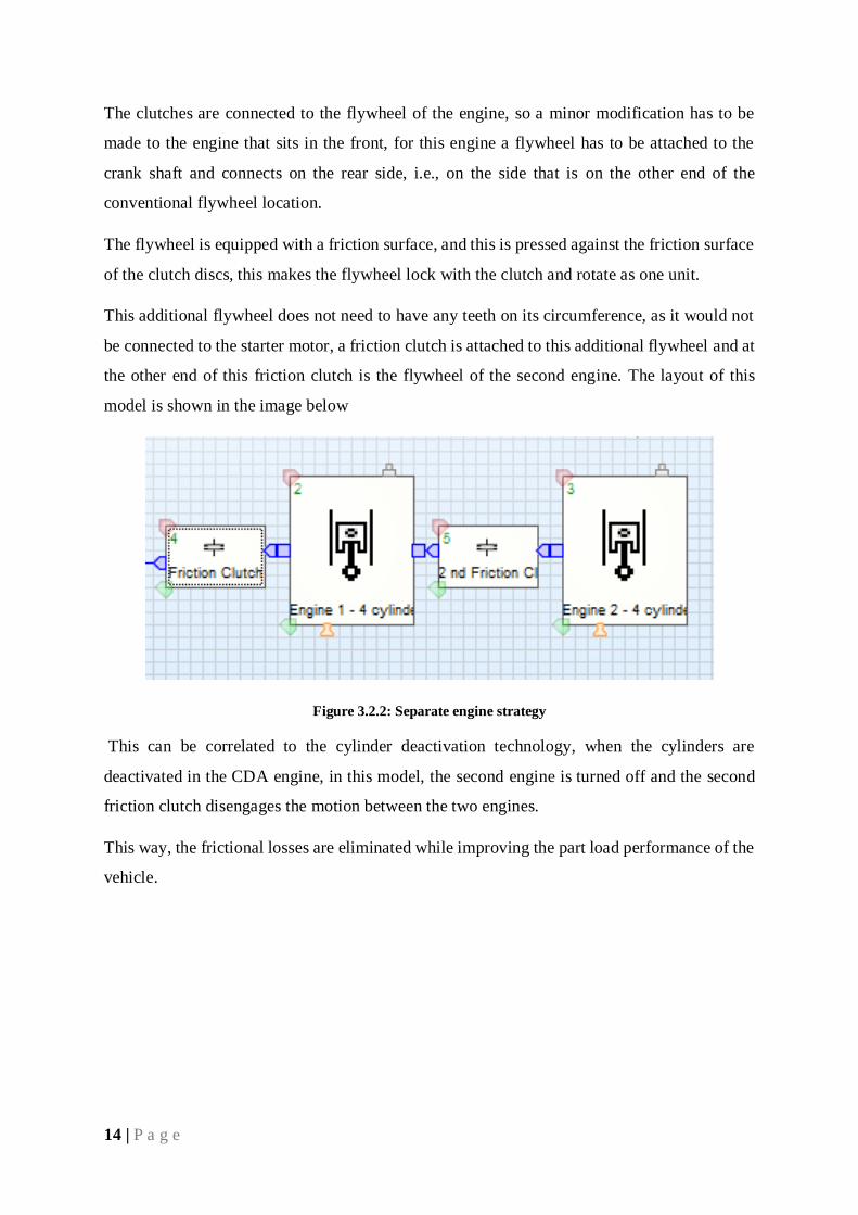
This additional flywheel does not need to have any teeth on its circumference, as it would not

be connected to the starter motor, a friction clutch is attached to this additional flywheel and at

the other end of this friction clutch is the flywheel of the second engine. The layout of this

model is shown in the image below

Figure 3.2.2: Separate engine strategy

This can be correlated to the cylinder deactivation technology, when the cylinders are

deactivated in the CDA engine, in this model, the second engine is turned off and the second

friction clutch disengages the motion between the two engines.

This way, the frictional losses are eliminated while improving the part load performance of the

vehicle.

15 | P a g e

4 Methodology

The proposed separate engine strategy is simulated and compared against the conventional

engine as well as cylinder deactivation engine and the fuel economy benefit if any, observed.

The following models are built for this project:

A 4-cylinder conventional engine

An 8-cylinder conventional engine

An 8-cylinder cylinder deactivation compatible engine

The following steps are taken to design and simulate in this project:

Firstly, the engine models are built in AVL BOOST software by defining the following

basic input data

o bore, stroke, number of cylinders, connecting rod length

o numbering of cylinders, principle arrangement of manifolds

o compression ratio, firing order and firing intervals

o number of valves, inner valve seat diameters

o valve lift curves

The simulated engine data from the first step, is input to the Vehicle model in AVL

CRUISE.

Modifications to the powertrain in case of the proposed separated engine technology is

accommodated by:

o Adding the moments of the additional flywheel to the first engine model

o Adding the weights of the additional components, used to accommodate this

proposed separate engine strategy, to the vehicle model

Running all the vehicle models through drive cycles, which simulate the real life driving

conditions.

Finally, comparing and analysing the results.

16 | P a g e

5 Engine Model Creation

5.1 AVL BOOST

BOOST is used for simulating a wide range of engines, spark ignited, compression ignited, 2 -

stroke or 4-stroke. The applications range from small capacity engines such as motorcycles up

to very large engines used for marine propulsion.

BOOST comes with an interactive pre-processor that helps in preparing the input data for the

main simulation program. An interactive post-processor supports the results analysis. The pre-

processor of AVL BOOST is equipped with a model editor. The computational model of an

engine is defined by using the element tree to select the required elements and these are

connected by piped elements. Availability of a wide range of elements make BOOST easier to

model complex engine configurations.

The BOOST program also provides optimized simulation algorithms for all the elements. The

pipe flow is treated as one-dimensional. This implies that the attributes related to flow such as

flow velocity, temperatures and pressures are obtained by solving the gas dynamic equations

which represent the mean values over the pipe cross-sections.

5.2 Creating the Model

AVL BOOST is used to create the following engine models.

A 4-Cylinder Conventional Engine

An 8-Cylinder Conventional Engine

An 8-Cylinder Engine having 4 cylinders deactivated

The first step to design an engine is to identify the required components, place them in the

working area and finally, complete the setup by providing the required connections in between

the components.

17 | P a g e

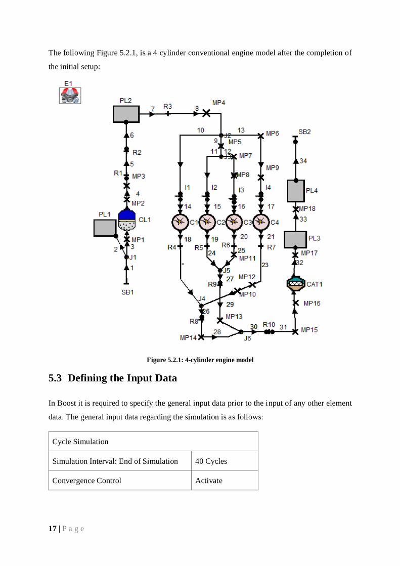
The following Figure 5.2.1, is a 4 cylinder conventional engine model after the completion of

the initial setup:

Figure 5.2.1: 4-cylinder engine model

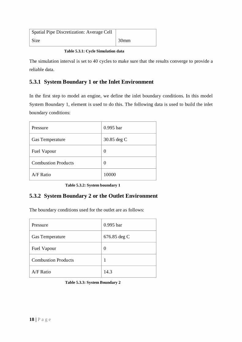
5.3 Defining the Input Data

In Boost it is required to specify the general input data prior to the input of any other element

data. The general input data regarding the simulation is as follows:

Cycle Simulation

Simulation Interval: End of Simulation 40 Cycles

Convergence Control Activate

18 | P a g e

Spatial Pipe Discretization: Average Cell

Size 30mm

Table 5.3.1: Cycle Simulation data

The simulation interval is set to 40 cycles to make sure that the results converge to provide a

reliable data.

5.3.1 System Boundary 1 or the Inlet Environment

In the first step to model an engine, we define the inlet boundary conditions. In this model

System Boundary 1, element is used to do this. The following data is used to build the inlet

boundary conditions:

Pressure 0.995 bar

Gas Temperature 30.85 deg C

Fuel Vapour 0

Combustion Products 0

A/F Ratio 10000

Table 5.3.2: System boundary 1

5.3.2 System Boundary 2 or the Outlet Environment

The boundary conditions used for the outlet are as follows:

Pressure 0.995 bar

Gas Temperature 676.85 deg C

Fuel Vapour 0

Combustion Products 1

A/F Ratio 14.3

Table 5.3.3: System Boundary 2

19 | P a g e

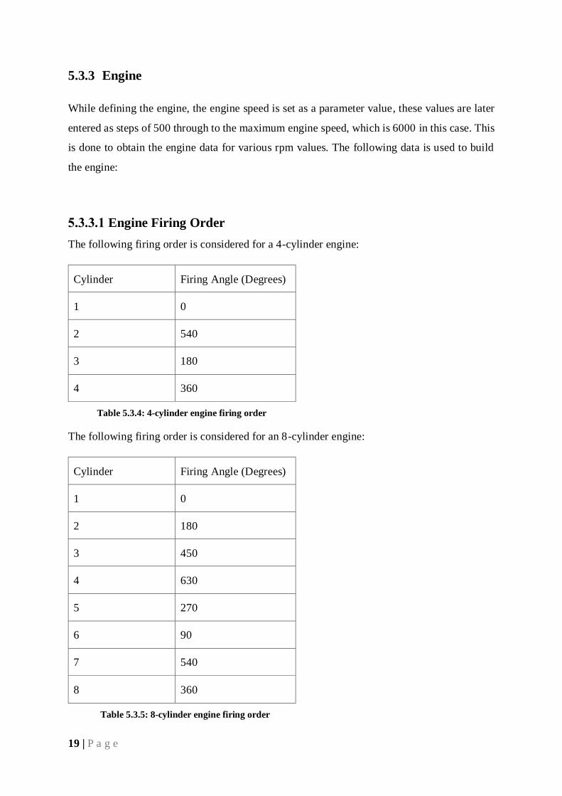
5.3.3 Engine

While defining the engine, the engine speed is set as a parameter value, these values are later

entered as steps of 500 through to the maximum engine speed, which is 6000 in this case. This

is done to obtain the engine data for various rpm values. The following data is used to build

the engine:

Engine Firing Order

The following firing order is considered for a 4-cylinder engine:

Cylinder Firing Angle (Degrees)

1 0

2 540

3 180

4 360

Table 5.3.4: 4-cylinder engine firing order

The following firing order is considered for an 8-cylinder engine:

Cylinder Firing Angle (Degrees)

1 0

2 180

3 450

4 630

5 270

6 90

7 540

8 360

Table 5.3.5: 8-cylinder engine firing order

20 | P a g e

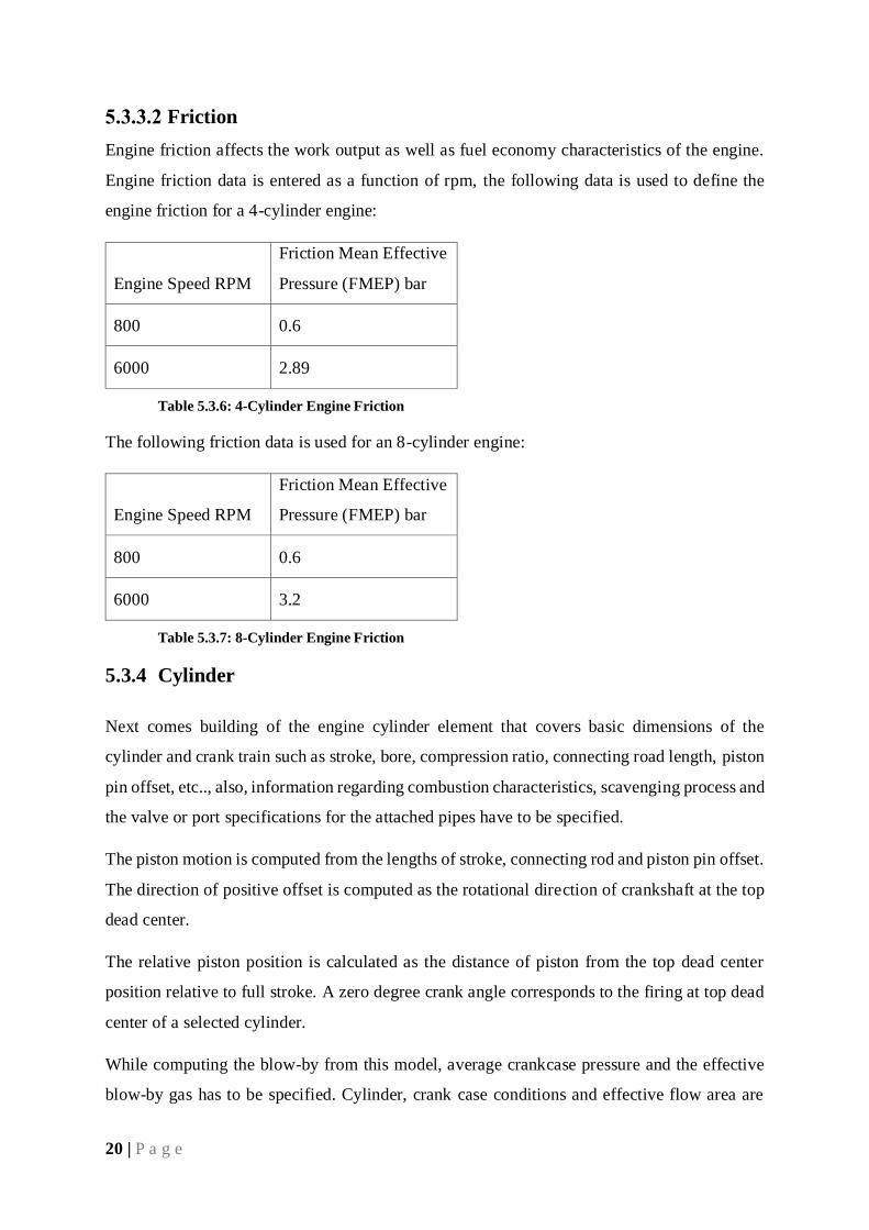
Friction

Engine friction affects the work output as well as fuel economy characteristics of the engine.

Engine friction data is entered as a function of rpm, the following data is used to define the

engine friction for a 4-cylinder engine:

Engine Speed RPM

Friction Mean Effective

Pressure (FMEP) bar

800 0.6

6000 2.89

Table 5.3.6: 4-Cylinder Engine Friction

The following friction data is used for an 8-cylinder engine:

Engine Speed RPM

Friction Mean Effective

Pressure (FMEP) bar

800 0.6

6000 3.2

Table 5.3.7: 8-Cylinder Engine Friction

5.3.4 Cylinder

Next comes building of the engine cylinder element that covers basic dimensions of the

cylinder and crank train such as stroke, bore, compression ratio, connecting road length, piston

pin offset, etc.., also, information regarding combustion characteristics, scavenging process and

the valve or port specifications for the attached pipes have to be specified.

The piston motion is computed from the lengths of stroke, connecting rod and piston pin offset.

The direction of positive offset is computed as the rotational direction of crankshaft at the top

dead center.

The relative piston position is calculated as the distance of piston from the top dead center

position relative to full stroke. A zero degree crank angle corresponds to the firing at top dead

center of a selected cylinder.

While computing the blow-by from this model, average crankcase pressure and the effective

blow-by gas has to be specified. Cylinder, crank case conditions and effective flow area are

21 | P a g e

used to calculate the actual blow-by mass. To calculate the effective flow area, cylinder

circumference and effective blow-by gap are considered.

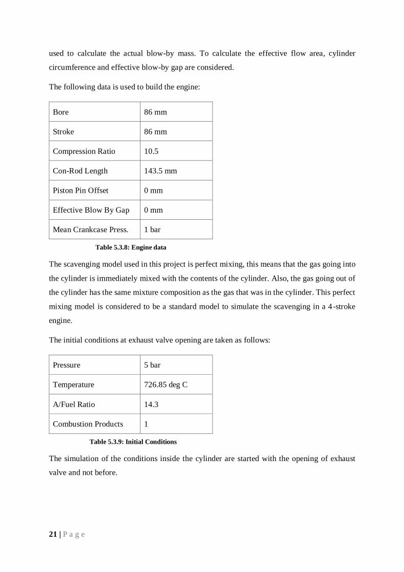
The following data is used to build the engine:

Bore 86 mm

Stroke 86 mm

Compression Ratio 10.5

Con-Rod Length 143.5 mm

Piston Pin Offset 0 mm

Effective Blow By Gap 0 mm

Mean Crankcase Press. 1 bar

Table 5.3.8: Engine data

The scavenging model used in this project is perfect mixing, this means that the gas going into

the cylinder is immediately mixed with the contents of the cylinder. Also, the gas going out of

the cylinder has the same mixture composition as the gas that was in the cylinder. This perfect

mixing model is considered to be a standard model to simulate the scavenging in a 4 -stroke

engine.

The initial conditions at exhaust valve opening are taken as follows:

Pressure 5 bar

Temperature 726.85 deg C

A/Fuel Ratio 14.3

Combustion Products 1

Table 5.3.9: Initial Conditions

The simulation of the conditions inside the cylinder are started with the opening of exhaust

valve and not before.

22 | P a g e

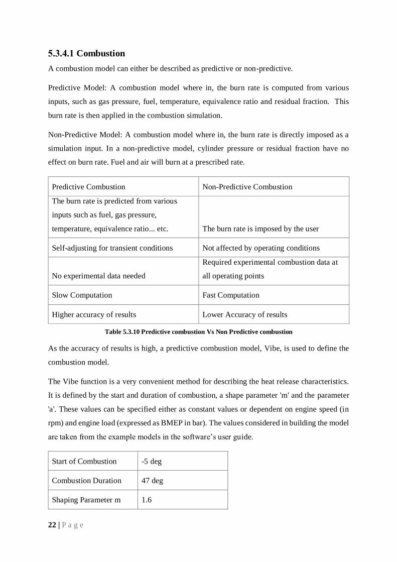
Combustion

A combustion model can either be described as predictive or non-predictive.

Predictive Model: A combustion model where in, the burn rate is computed from various

inputs, such as gas pressure, fuel, temperature, equivalence ratio and residual fraction. This

burn rate is then applied in the combustion simulation.

Non-Predictive Model: A combustion model where in, the burn rate is directly imposed as a

simulation input. In a non-predictive model, cylinder pressure or residual fraction have no

effect on burn rate. Fuel and air will burn at a prescribed rate.

Predictive Combustion Non-Predictive Combustion

The burn rate is predicted from various

inputs such as fuel, gas pressure,

temperature, equivalence ratio... etc. The burn rate is imposed by the user

Self-adjusting for transient conditions Not affected by operating conditions

No experimental data needed

Required experimental combustion data at

all operating points

Slow Computation Fast Computation

Higher accuracy of results Lower Accuracy of results

Table 5.3.10 Predictive combustion Vs Non Predictive combustion

As the accuracy of results is high, a predictive combustion model, Vibe, is used to define the

combustion model.

The Vibe function is a very convenient method for describing the heat release characteristics.

It is defined by the start and duration of combustion, a shape parameter 'm' and the parameter

'a'. These values can be specified either as constant values or dependent on engine speed (in

rpm) and engine load (expressed as BMEP in bar). The values considered in building the model

are taken from the example models in the software’s user guide.

Start of Combustion -5 deg

Combustion Duration 47 deg

Shaping Parameter m 1.6

23 | P a g e

Parameter a 6.9

Table 5.3.11: Combustion Model

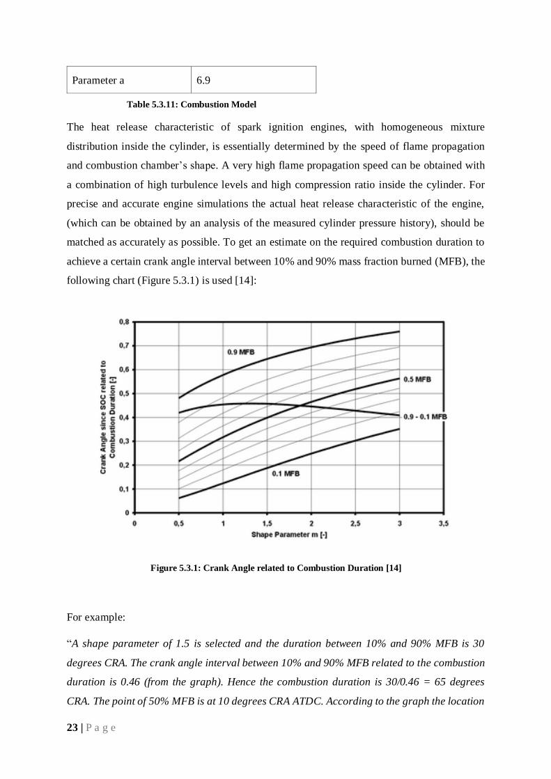
The heat release characteristic of spark ignition engines, with homogeneous mixture

distribution inside the cylinder, is essentially determined by the speed of flame propagation

and combustion chamber’s shape. A very high flame propagation speed can be obtained with

a combination of high turbulence levels and high compression ratio inside the cylinder. For

precise and accurate engine simulations the actual heat release characteristic of the engine,

(which can be obtained by an analysis of the measured cylinder pressure history), should be

matched as accurately as possible. To get an estimate on the required combustion duration to

achieve a certain crank angle interval between 10% and 90% mass fraction burned (MFB), the

following chart (Figure 5.3.1) is used [14]:

Figure 5.3.1: Crank Angle related to Combustion Duration [14]

For example:

“A shape parameter of 1.5 is selected and the duration between 10% and 90% MFB is 30

degrees CRA. The crank angle interval between 10% and 90% MFB related to the combustion

duration is 0.46 (from the graph). Hence the combustion duration is 30/0.46 = 65 degrees

CRA. The point of 50% MFB is at 10 degrees CRA ATDC. According to the graph the location

24 | P a g e

of 50 % MFB after combustion start related to the combustion duration is 0.4. Thus the

combustion start is calculated from 10 - 65 * 0.4 = -16 = 16 degrees BTDC” [14].

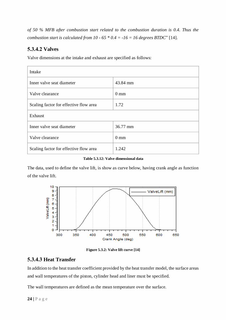
Valves

Valve dimensions at the intake and exhaust are specified as follows:

Intake

Inner valve seat diameter 43.84 mm

Valve clearance 0 mm

Scaling factor for effective flow area 1.72

Exhaust

Inner valve seat diameter 36.77 mm

Valve clearance 0 mm

Scaling factor for effective flow area 1.242

Table 5.3.12: Valve dimensional data

The data, used to define the valve lift, is show as curve below, having crank angle as function

of the valve lift.

Figure 5.3.2: Valve lift curve [14]

Heat Transfer

In addition to the heat transfer coefficient provided by the heat transfer model, the surface areas

and wall temperatures of the piston, cylinder head and liner must be specified.

The wall temperatures are defined as the mean temperature over the surface.

25 | P a g e

A calibration factor for each surface may be used to increase or to reduce the heat transfer.

For the surface areas the following values are considered:

5.3.4.3.1 Piston:

SI engines: Surface area is approximately equal to the bore area.

5.3.4.3.2 Cylinder Head:

SI engines: Surface area is approximately 1.1 times the bore area.

5.3.4.3.3 Liner with Piston at TDC:

The area may be calculated from an estimated piston to head clearance times the circumference

of the cylinder. The mean effective thickness of the piston, the liner and the fire deck of the

cylinder head together with the heat capacity determine the thermal inertia of the combustion

chamber walls. The conductivity is required to calculate the temperature difference between

the surface facing the combustion chamber and the surface facing the coolant.

The heat capacity is the product of the density and the specific heat of the material.

For the heat transfer to the coolant (head and liner) and engine oil (piston), an average heat

transfer coefficient and the temperature of the medium must be specified [14].

To build the heat transfer model, all the surface areas of piston, cylinder head and liners are

defined as follows:

Heat Transfer

Cylinder Model Woschni 1978

Piston

Surface Area 5809 mm2

Wall Temperature 226.85 degC

Piston Calibration Factor 1

Cylinder Head

Surface Area 7550 m2

26 | P a g e

Wall Temperature 256.85 degC

Head Calibration Factor 1

Liner

Surface Area when piston at TDC 270 mm2

Wall Temperature when piston at TDC 161.85 degC

Wall Temperature when piston at BDC 151.85 degC

Liner Calibration Factor 1

Combustion System Direct Ignition

In-cylinder Swirl Ratio 0

Table 5.3.13: Heat transfer model

5.3.5 Injector

An injector was defined by specifying the air fuel ratio to 13.34 and a continuous injection

method is selected as the injector model.

5.3.6 Air Cleaner

The total volume of the air cleaner, the collector volumes of the collectors at inlet and outlet

and the filter element’s length have to be define during air cleaner modelling. The following

data is considered to build an air cleaner:

Air Cleaner

Geometrical Properties

Total Air Cleaner Volume 8.7 litres

Inlet Collector Volume 3.0 litres

Outlet Collector Volume 4.3 litres

Length of Filter Element 300 mm

Friction Specification Target Pressure Drop

27 | P a g e

Target Pressure Drop

Mass Flow 0.13 kg/s

Target Pressure Drop 0.008 bar

Inlet Pressure 1 bar

Inlet Air Temperature 19.85 degC

Table 5.3.14: Air cleaner data

The filter element’s length is used to model the time required by the pressure wave to travel

throughout the air cleaner.

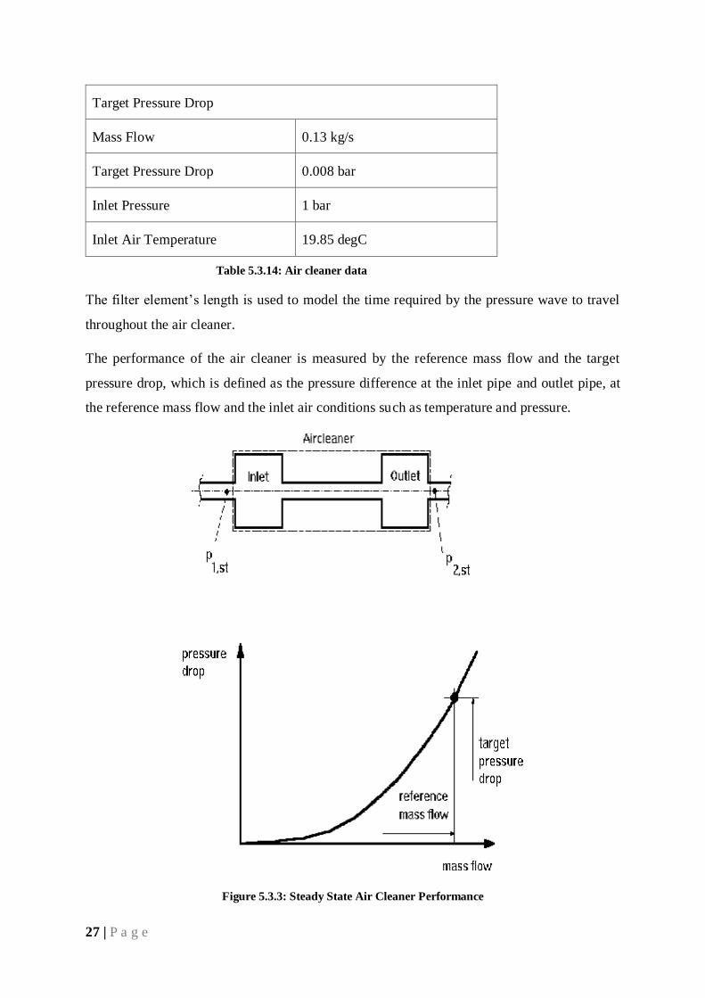
The performance of the air cleaner is measured by the reference mass flow and the target

pressure drop, which is defined as the pressure difference at the inlet pipe and outlet pipe, at

the reference mass flow and the inlet air conditions such as temperature and pressure.

Figure 5.3.3: Steady State Air Cleaner Performance

28 | P a g e

With reference to the above information, the program adjusts the wall friction loss in the

model accordingly.

5.3.7 Junctions

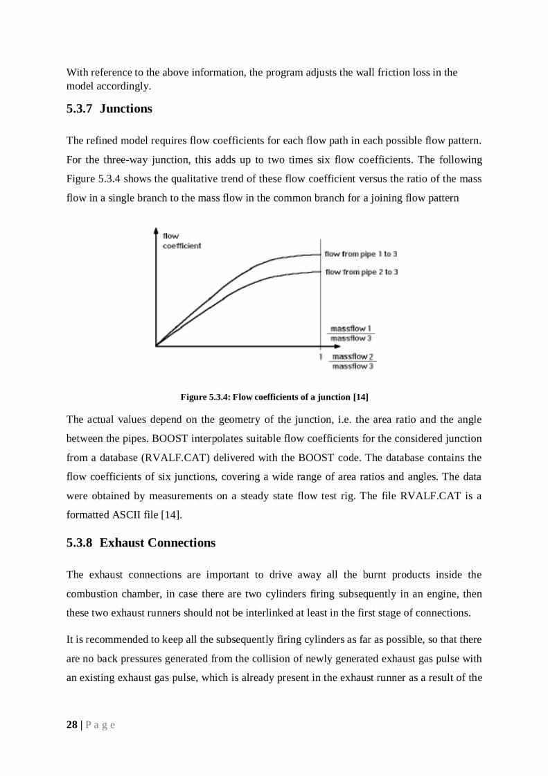
The refined model requires flow coefficients for each flow path in each possible flow pattern.

For the three-way junction, this adds up to two times six flow coefficients. The following

Figure 5.3.4 shows the qualitative trend of these flow coefficient versus the ratio of the mass

flow in a single branch to the mass flow in the common branch for a joining flow pattern

Figure 5.3.4: Flow coefficients of a junction [14]

The actual values depend on the geometry of the junction, i.e. the area ratio and the angle

between the pipes. BOOST interpolates suitable flow coefficients for the considered junction

from a database (RVALF.CAT) delivered with the BOOST code. The database contains the

flow coefficients of six junctions, covering a wide range of area ratios and angles. The data

were obtained by measurements on a steady state flow test rig. The file RVALF.CAT is a

formatted ASCII file [14].

5.3.8 Exhaust Connections

The exhaust connections are important to drive away all the burnt products inside the

combustion chamber, in case there are two cylinders firing subsequently in an engine, then

these two exhaust runners should not be interlinked at least in the first stage of connections.

It is recommended to keep all the subsequently firing cylinders as far as possible, so that there

are no back pressures generated from the collision of newly generated exhaust gas pulse with

an existing exhaust gas pulse, which is already present in the exhaust runner as a result of the

29 | P a g e

previous power stroke in the first cylinder, this affects the efficiency of the engine to drive

away the combustion products from the chamber.

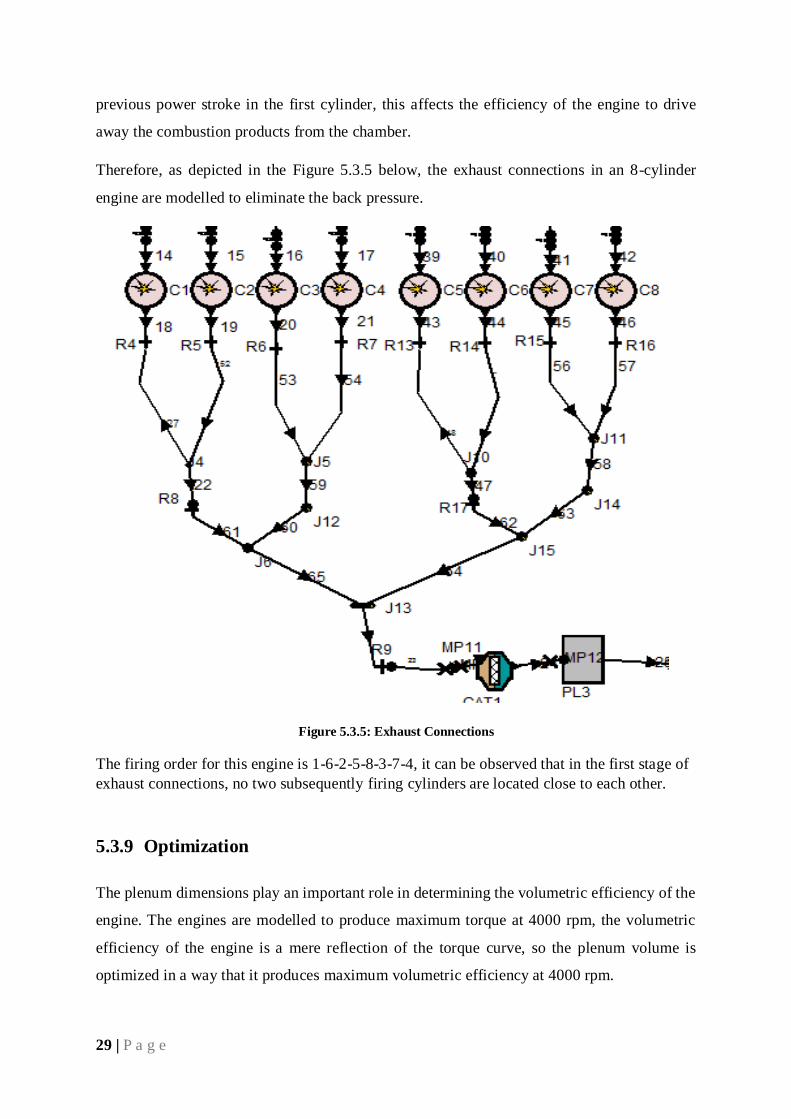
Therefore, as depicted in the Figure 5.3.5 below, the exhaust connections in an 8-cylinder

engine are modelled to eliminate the back pressure.

Figure 5.3.5: Exhaust Connections

The firing order for this engine is 1-6-2-5-8-3-7-4, it can be observed that in the first stage of

exhaust connections, no two subsequently firing cylinders are located close to each other.

5.3.9 Optimization

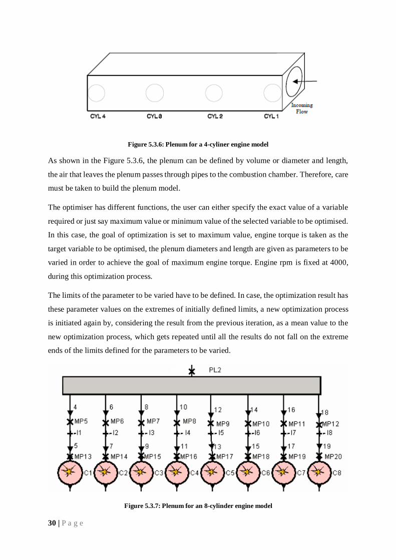
The plenum dimensions play an important role in determining the volumetric efficiency of the

engine. The engines are modelled to produce maximum torque at 4000 rpm, the volumetric

efficiency of the engine is a mere reflection of the torque curve, so the plenum volume is

optimized in a way that it produces maximum volumetric efficiency at 4000 rpm.

30 | P a g e

Figure 5.3.6: Plenum for a 4-cyliner engine model

As shown in the Figure 5.3.6, the plenum can be defined by volume or diameter and length,

the air that leaves the plenum passes through pipes to the combustion chamber. Therefore, care

must be taken to build the plenum model.

The optimiser has different functions, the user can either specify the exact value of a variable

required or just say maximum value or minimum value of the selected variable to be optimised.

In this case, the goal of optimization is set to maximum value, engine torque is taken as the

target variable to be optimised, the plenum diameters and length are given as parameters to be

varied in order to achieve the goal of maximum engine torque. Engine rpm is fixed at 4000,

during this optimization process.

The limits of the parameter to be varied have to be defined. In case, the optimization result has

these parameter values on the extremes of initially defined limits, a new optimization process

is initiated again by, considering the result from the previous iteration, as a mean value to the

new optimization process, which gets repeated until all the results do not fall on the extreme

ends of the limits defined for the parameters to be varied.

Figure 5.3.7: Plenum for an 8-cylinder engine model

31 | P a g e

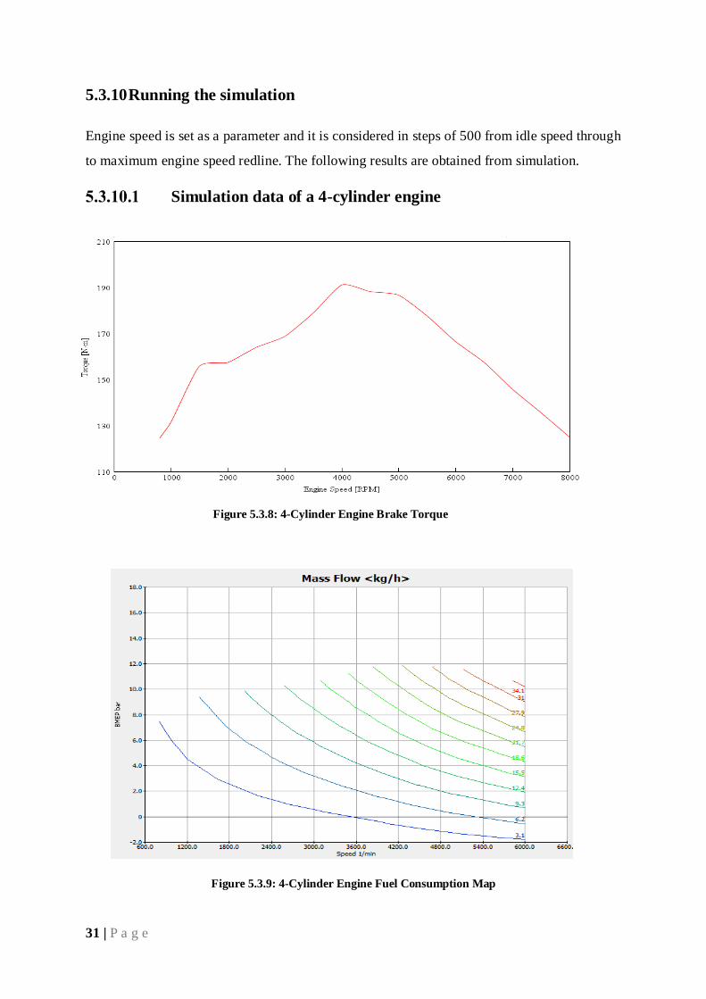
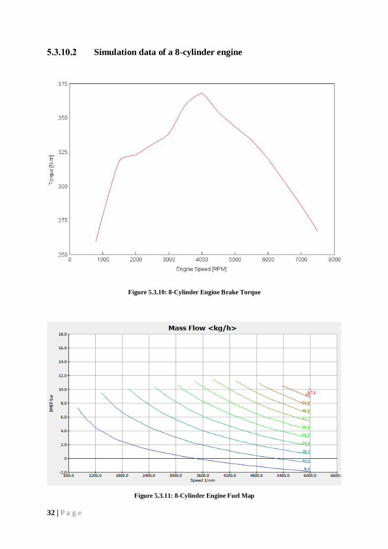
5.3.10 Running the simulation

Engine speed is set as a parameter and it is considered in steps of 500 from idle speed through

to maximum engine speed redline. The following results are obtained from simulation.

Simulation data of a 4-cylinder engine

Figure 5.3.9: 4-Cylinder Engine Fuel Consumption Map

Figure 5.3.8: 4-Cylinder Engine Brake Torque

32 | P a g e

Simulation data of a 8-cylinder engine

Figure 5.3.10: 8-Cylinder Engine Brake Torque

Figure 5.3.11: 8-Cylinder Engine Fuel Map

33 | P a g e

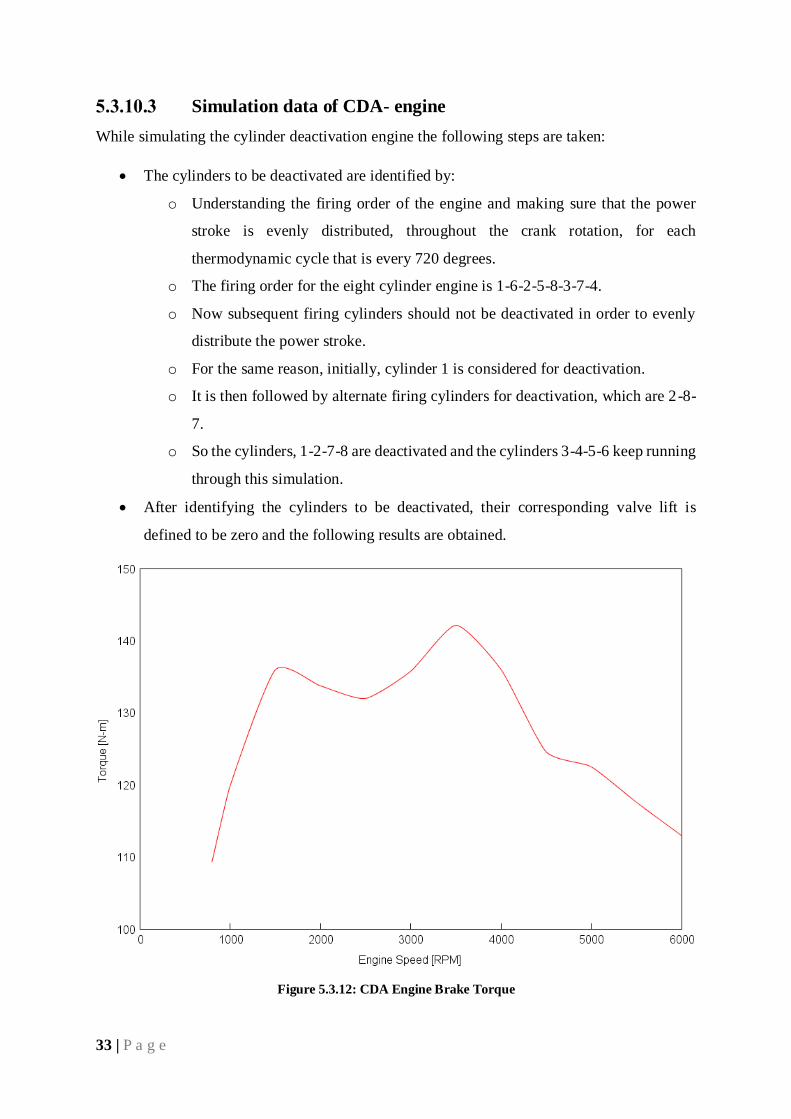
Simulation data of CDA- engine

While simulating the cylinder deactivation engine the following steps are taken:

The cylinders to be deactivated are identified by:

o Understanding the firing order of the engine and making sure that the power

stroke is evenly distributed, throughout the crank rotation, for each

thermodynamic cycle that is every 720 degrees.

o The firing order for the eight cylinder engine is 1-6-2-5-8-3-7-4.

o Now subsequent firing cylinders should not be deactivated in order to evenly

distribute the power stroke.

o For the same reason, initially, cylinder 1 is considered for deactivation.

o It is then followed by alternate firing cylinders for deactivation, which are 2-8-

7.

o So the cylinders, 1-2-7-8 are deactivated and the cylinders 3-4-5-6 keep running

through this simulation.

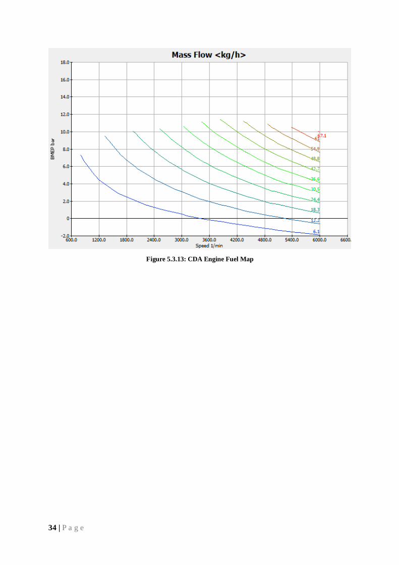
After identifying the cylinders to be deactivated, their corresponding valve lift is

defined to be zero and the following results are obtained.

Figure 5.3.12: CDA Engine Brake Torque

34 | P a g e

Figure 5.3.13: CDA Engine Fuel Map

35 | P a g e

6 Running Simulation Using AVL CRUISE

6.1 AVL CRUISE

AVL CRUISE is a system level simulation software used to simulate vehicle and powertrain.

It supports day to day tasks in a vehicle, powertrain analysis, through the entire development

phase, right from concept planning until the launch and beyond. Its application range covers

conventional drivelines through to advanced hybrid powertrain systems and purely electric

drivelines. It provides a streamlined workflow for various kinds of parameter optimizations

and component matching which aid the user in attainable and practical solutions. It has

organised interface, highly advanced data management scheme, also well equipped with system

integration and data communication which have established CRUISE as a world leader and is

being used by major OEM’s and suppliers.

To summarise, CRUISE is used in engine development and drivetrain to calculate and optimize

the following:

Fuel Consumption

Driving Performance

Transmission ratios

Braking Performance

6.2 CRUISE Workflow

The following steps are referred for the CRUISE workflow:

Create project/version

Create vehicle model

Input the data in components

Create connections: Energetic

Create connections: Informational

Create task folders and add tasks

Set up calculation

Run calculation

View and evaluate results

36 | P a g e

6.3 Creating the Vehicle Model

The following components are placed in the work area and each of them are defined

individually

• Vehicle

• Engine

• Clutch

• Gear Box

• Single Ratio Transmission

• Differential

• 4 Brakes

• 4 Wheels

• Cockpit

• Monitor

6.3.1 Defining the Input Data for each component

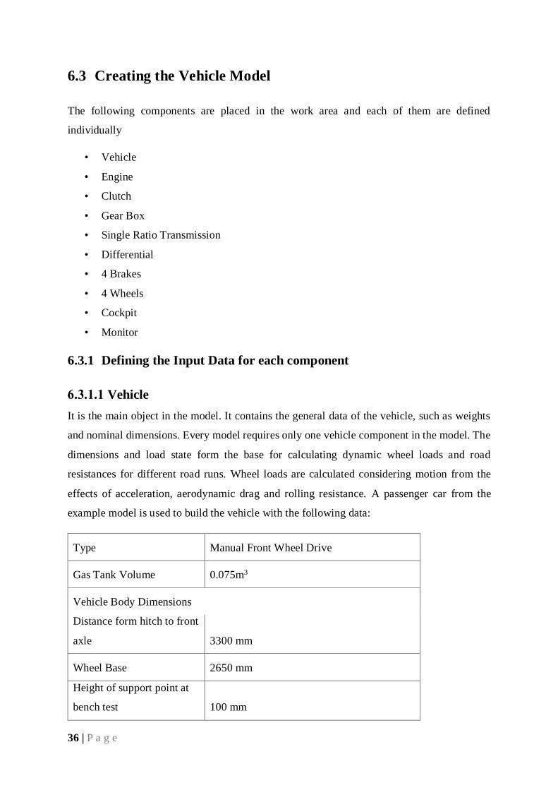
Vehicle

It is the main object in the model. It contains the general data of the vehicle, such as weights

and nominal dimensions. Every model requires only one vehicle component in the model. The

dimensions and load state form the base for calculating dynamic wheel loads and road

resistances for different road runs. Wheel loads are calculated considering motion from the

effects of acceleration, aerodynamic drag and rolling resistance. A passenger car from the

example model is used to build the vehicle with the following data:

Type Manual Front Wheel Drive

Gas Tank Volume 0.075m3

Vehicle Body Dimensions

Distance form hitch to front

axle 3300 mm

Wheel Base 2650 mm

Height of support point at

bench test 100 mm

37 | P a g e

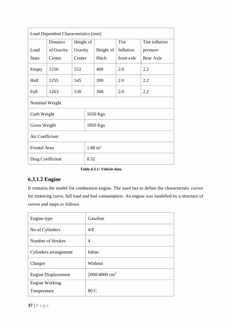
Load Dependent Characteristics [mm]

Load

State

Distance

of Gravity

Center

Height of

Gravity

Center

Height of

Hitch

Tire

Inflation

front axle

Tire inflation

pressure

Rear Axle

Empty 1250 552 400 2.0 2.2

Half 1255 545 390 2.0 2.2

Full 1263 530 368 2.0 2.2

Nominal Weight

Curb Weight 1650 Kgs

Gross Weight 1850 Kgs

Air Coefficient

Frontal Area 1.88 m2

Drag Coefficient 0.32

Table 6.3.1: Vehicle data

Engine

It contains the model for combustion engine. The used has to define the characteristic curves

for motoring curve, full load and fuel consumption. An engine was modelled by a structure of

curves and maps as follows

Engine type Gasoline

No of Cylinders 4/8

Number of Strokes 4

Cylinders arrangement Inline

Charger Without

Engine Displacement 2000/4000 cm3

Engine Working

Temperature 80 C

38 | P a g e

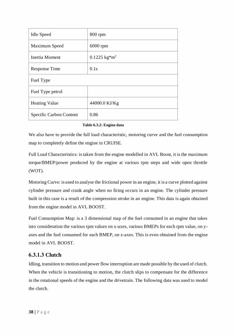
Idle Speed 800 rpm

Maximum Speed 6000 rpm

Inertia Moment 0.1225 kg*m2

Response Time 0.1s

Fuel Type

Fuel Type petrol

Heating Value 44000.0 KJ/Kg

Specific Carbon Content 0.86

Table 6.3.2: Engine data

We also have to provide the full load characteristic, motoring curve and the fuel consumption

map to completely define the engine in CRUISE.

Full Load Characteristics: is taken from the engine modelled in AVL Boost, it is the maximum

torque/BMEP/power produced by the engine at various rpm steps and wide open throttle

(WOT).

Motoring Curve: is used to analyse the frictional power in an engine, it is a curve plotted against

cylinder pressure and crank angle when no firing occurs in an engine. The cylinder pressure

built in this case is a result of the compression stroke in an engine. This data is again obtained

from the engine model in AVL BOOST.

Fuel Consumption Map: is a 3 dimensional map of the fuel consumed in an engine that takes

into consideration the various rpm values on x-axes, various BMEPs for each rpm value, on y-

axes and the fuel consumed for each BMEP, on z-axes. This is even obtained from the engine

model in AVL BOOST.

Clutch

Idling, transition to motion and power flow interruption are made possible by the used of clutch.

When the vehicle is transitioning to motion, the clutch slips to compensate for the difference

in the rotational speeds of the engine and the drivetrain. The following data was used to model

the clutch.

39 | P a g e

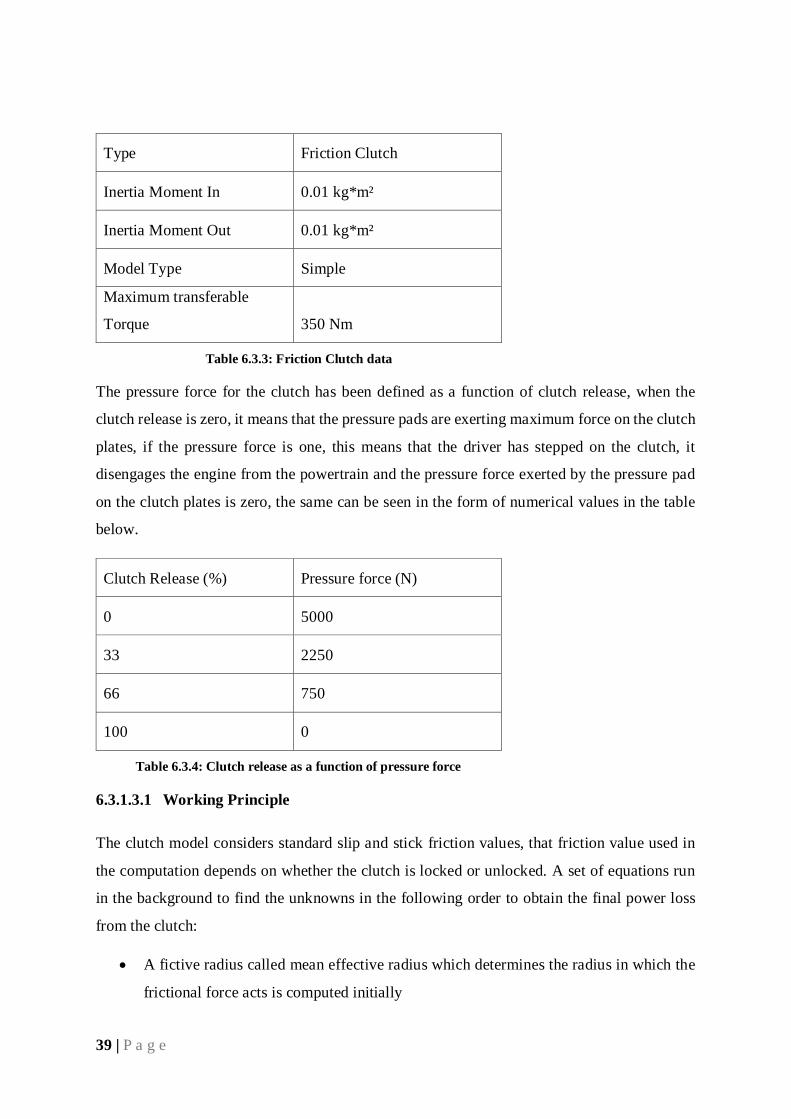
Type Friction Clutch

Inertia Moment In 0.01 kg*m²

Inertia Moment Out 0.01 kg*m²

Model Type Simple

Maximum transferable

Torque 350 Nm

Table 6.3.3: Friction Clutch data

The pressure force for the clutch has been defined as a function of clutch release, when the

clutch release is zero, it means that the pressure pads are exerting maximum force on the clutch

plates, if the pressure force is one, this means that the driver has stepped on the clutch, it

disengages the engine from the powertrain and the pressure force exerted by the pressure pad

on the clutch plates is zero, the same can be seen in the form of numerical values in the table

below.

Clutch Release (%) Pressure force (N)

0 5000

33 2250

66 750

100 0

Table 6.3.4: Clutch release as a function of pressure force

6.3.1.3.1 Working Principle

The clutch model considers standard slip and stick friction values, that friction value used in

the computation depends on whether the clutch is locked or unlocked. A set of equations run

in the background to find the unknowns in the following order to obtain the final power loss

from the clutch:

A fictive radius called mean effective radius which determines the radius in which the

frictional force acts is computed initially

40 | P a g e

The actual frictional coefficient is then calculated from the relative angular velocity and

a function of stick and slip frictional coefficients

Later, the transmitted torque in a clutch is calculated by interpolating the actual

clamping force from the actual clutch release map and by multiplying the obtained

value with the above calculated values

Finally, the power loss in a clutch is evaluated from the difference in powers at the inlet

and output of the clutch

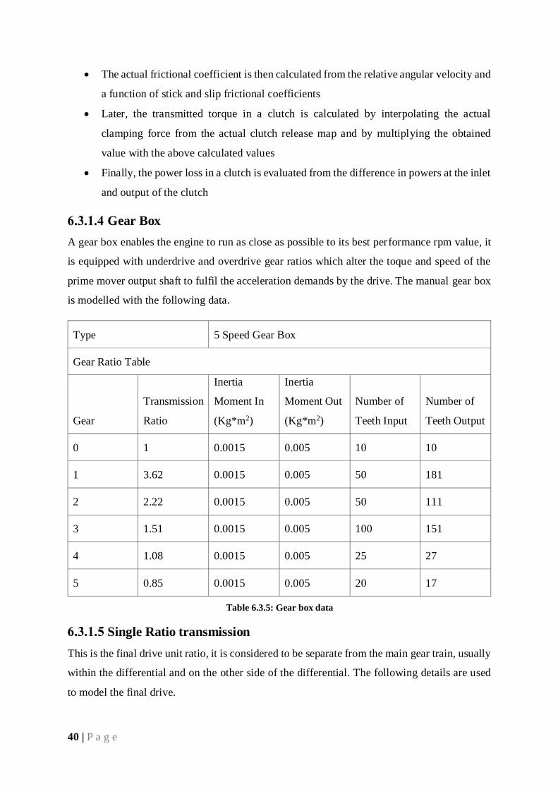
Gear Box

A gear box enables the engine to run as close as possible to its best performance rpm value, it

is equipped with underdrive and overdrive gear ratios which alter the toque and speed of the

prime mover output shaft to fulfil the acceleration demands by the drive. The manual gear box

is modelled with the following data.

Type 5 Speed Gear Box

Gear Ratio Table

Gear

Transmission

Ratio

Inertia

Moment In

(Kg*m2)

Inertia

Moment Out

(Kg*m2)

Number of

Teeth Input

Number of

Teeth Output

0 1 0.0015 0.005 10 10

1 3.62 0.0015 0.005 50 181

2 2.22 0.0015 0.005 50 111

3 1.51 0.0015 0.005 100 151

4 1.08 0.0015 0.005 25 27

5 0.85 0.0015 0.005 20 17

Table 6.3.5: Gear box data

Single Ratio transmission

This is the final drive unit ratio, it is considered to be separate from the main gear train, usually

within the differential and on the other side of the differential. The following details are used

to model the final drive.

41 | P a g e

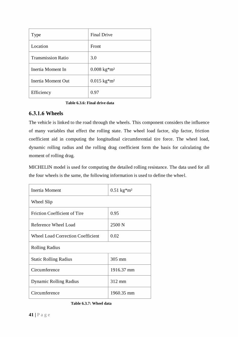
Type Final Drive

Location Front

Transmission Ratio 3.0

Inertia Moment In 0.008 kg*m²

Inertia Moment Out 0.015 kg*m²

Efficiency 0.97

Table 6.3.6: Final drive data

Wheels

The vehicle is linked to the road through the wheels. This component considers the influence

of many variables that effect the rolling state. The wheel load factor, slip factor, friction

coefficient aid in computing the longitudinal circumferential tire force. The wheel load,

dynamic rolling radius and the rolling drag coefficient form the basis for calculating the

moment of rolling drag.

MICHELIN model is used for computing the detailed rolling resistance. The data used for all

the four wheels is the same, the following information is used to define the wheel.

Inertia Moment 0.51 kg*m²

Wheel Slip

Friction Coefficient of Tire 0.95

Reference Wheel Load 2500 N

Wheel Load Correction Coefficient 0.02

Rolling Radius

Static Rolling Radius 305 mm

Circumference 1916.37 mm

Dynamic Rolling Radius 312 mm

Circumference 1960.35 mm

Table 6.3.7: Wheel data

42 | P a g e

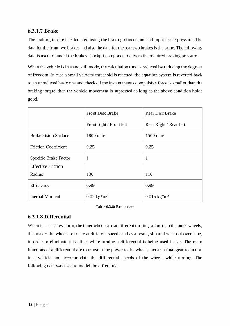
Brake

The braking torque is calculated using the braking dimensions and input brake pressure. The

data for the front two brakes and also the data for the rear two brakes is the same. The following

data is used to model the brakes. Cockpit component delivers the required braking pressure.

When the vehicle is in stand still mode, the calculation time is reduced by reducing the degrees

of freedom. In case a small velocity threshold is reached, the equation system is reverted back

to an unreduced basic one and checks if the instantaneous compulsive force is smaller than the

braking torque, then the vehicle movement is supressed as long as the above condition holds

good.

Front Disc Brake Rear Disc Brake

Front right / Front left Rear Right / Rear left

Brake Piston Surface 1800 mm² 1500 mm²

Friction Coefficient 0.25 0.25

Specific Brake Factor 1 1

Effective Friction

Radius 130 110

Efficiency 0.99 0.99

Inertial Moment 0.02 kg*m² 0.015 kg*m²

Table 6.3.8: Brake data

Differential

When the car takes a turn, the inner wheels are at different turning radius than the outer wheels,

this makes the wheels to rotate at different speeds and as a result, slip and wear out over time,

in order to eliminate this effect while turning a differential is being used in car. The main

functions of a differential are to transmit the power to the wheels, act as a final gear reduction

in a vehicle and accommodate the differential speeds of the wheels while turning. The

following data was used to model the differential.

43 | P a g e

Type Differential

Location Front end

Differential Lock Unlocked

Torque Split Factor 1

Inertia Moment In 0.015 kg*m²

Inertia Moment Out 0.015 kg*m²

Table 6.3.9: Differential data

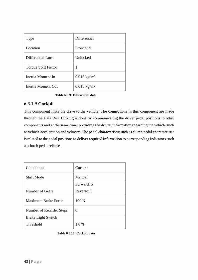
Cockpit

This component links the drive to the vehicle. The connections in this component are made

through the Data Bus. Linking is done by communicating the driver pedal positions to other

components and at the same time, providing the driver, information regarding the vehicle such

as vehicle acceleration and velocity. The pedal characteristic such as clutch pedal characteristic

is related to the pedal positions to deliver required information to corresponding indicators such

as clutch pedal release.

Component Cockpit

Shift Mode Manual

Number of Gears

Forward: 5

Reverse: 1

Maximum Brake Force 100 N

Number of Retarder Steps 0

Brake Light Switch

Threshold 1.0 %

Table 6.3.10: Cockpit data

44 | P a g e

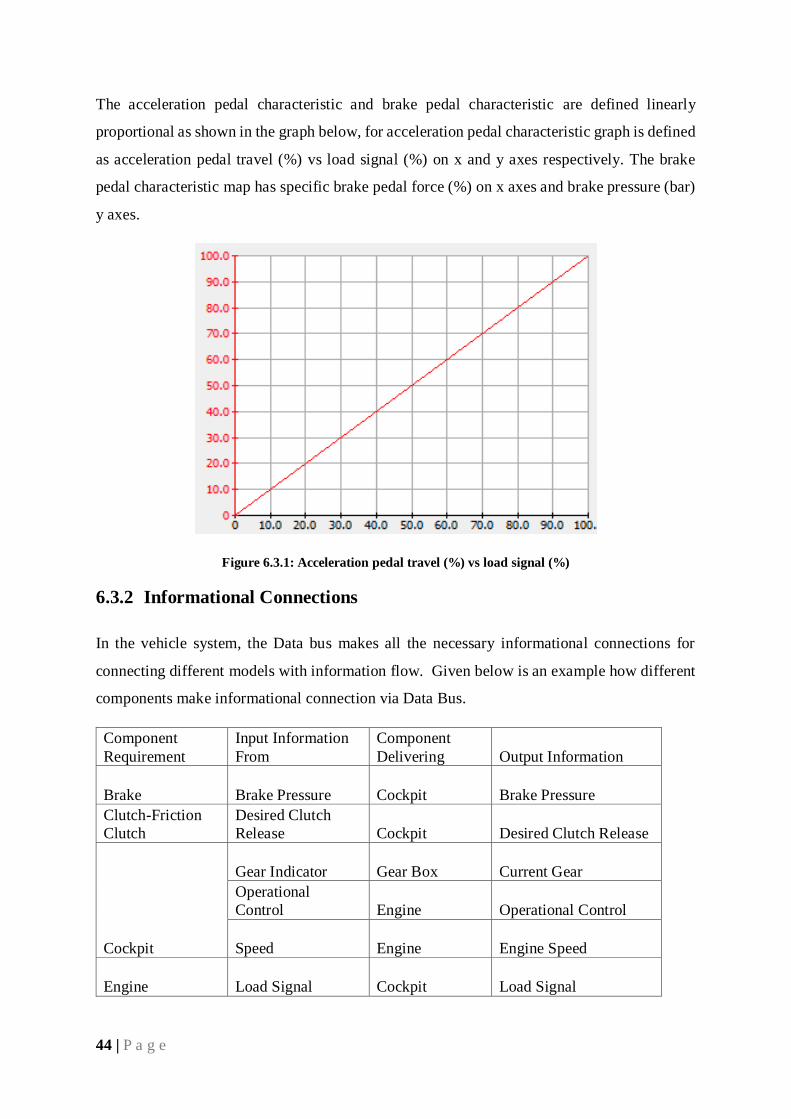
The acceleration pedal characteristic and brake pedal characteristic are defined linearly

proportional as shown in the graph below, for acceleration pedal characteristic graph is defined

as acceleration pedal travel (%) vs load signal (%) on x and y axes respectively. The brake

pedal characteristic map has specific brake pedal force (%) on x axes and brake pressure (bar)

y axes.

Figure 6.3.1: Acceleration pedal travel (%) vs load signal (%)

6.3.2 Informational Connections

In the vehicle system, the Data bus makes all the necessary informational connections for

connecting different models with information flow. Given below is an example how different

components make informational connection via Data Bus.

Component

Requirement

Input Information

From

Component

Delivering Output Information

Brake Brake Pressure Cockpit Brake Pressure

Clutch-Friction

Clutch

Desired Clutch

Release Cockpit Desired Clutch Release

Cockpit

Gear Indicator Gear Box Current Gear

Operational

Control Engine Operational Control

Speed Engine Engine Speed

Engine Load Signal Cockpit Load Signal

45 | P a g e

Start Switch Cockpit Start Switch

Gear Box Desired Gear Cockpit Desired Gear

Table 6.3.11: Data bus connections

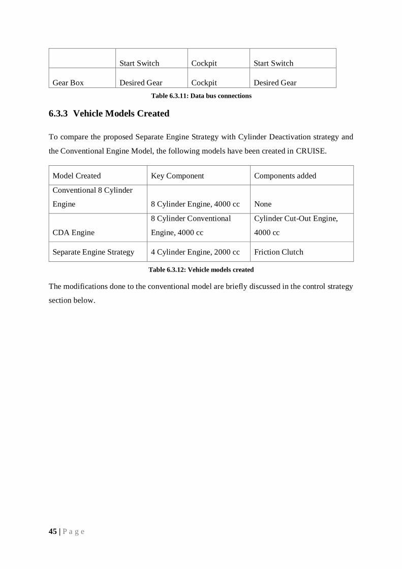
6.3.3 Vehicle Models Created

To compare the proposed Separate Engine Strategy with Cylinder Deactivation strategy and

the Conventional Engine Model, the following models have been created in CRUISE.

Model Created Key Component Components added

Conventional 8 Cylinder

Engine 8 Cylinder Engine, 4000 cc None

CDA Engine

8 Cylinder Conventional

Engine, 4000 cc

Cylinder Cut-Out Engine,

4000 cc

Separate Engine Strategy 4 Cylinder Engine, 2000 cc Friction Clutch

Table 6.3.12: Vehicle models created

The modifications done to the conventional model are briefly discussed in the control strategy

section below.

46 | P a g e

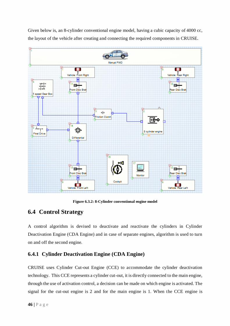
Given below is, an 8-cylinder conventional engine model, having a cubic capacity of 4000 cc,

the layout of the vehicle after creating and connecting the required components in CRUISE.

Figure 6.3.2: 8-Cylinder conventional engine model

6.4 Control Strategy

A control algorithm is devised to deactivate and reactivate the cylinders in Cylinder

Deactivation Engine (CDA Engine) and in case of separate engines, algorithm is used to turn

on and off the second engine.

6.4.1 Cylinder Deactivation Engine (CDA Engine)

CRUISE uses Cylinder Cut-out Engine (CCE) to accommodate the cylinder deactivation

technology. This CCE represents a cylinder cut-out, it is directly connected to the main engine,

through the use of activation control, a decision can be made on which engine is activated. The

signal for the cut-out engine is 2 and for the main engine is 1. When the CCE engine is

47 | P a g e

activated, some data such as full load characteristic and engine maps are taken from CCE

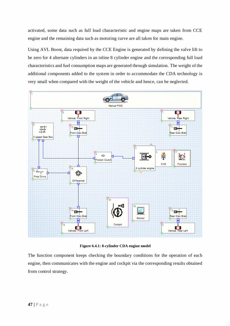
engine and the remaining data such as motoring curve are all taken for main engine.

Using AVL Boost, data required by the CCE Engine is generated by defining the valve lift to

be zero for 4 alternate cylinders in an inline 8 cylinder engine and the corresponding full load

characteristics and fuel consumption maps are generated through simulation. The weight of the

additional components added to the system in order to accommodate the CDA technology is

very small when compared with the weight of the vehicle and hence, can be neglected.

Figure 6.4.1: 8-cylinder CDA engine model

The function component keeps checking the boundary conditions for the operation of each

engine, then communicates with the engine and cockpit via the corresponding results obtained

from control strategy.

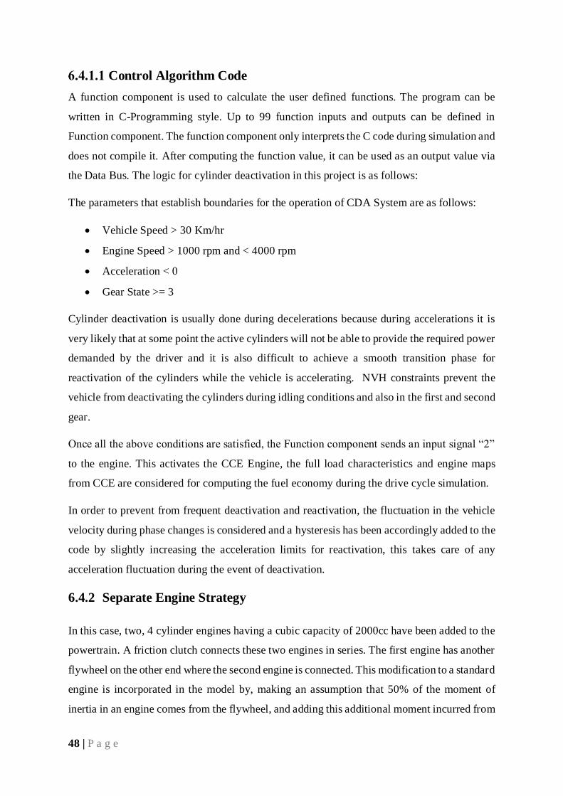
48 | P a g e

Control Algorithm Code

A function component is used to calculate the user defined functions. The program can be

written in C-Programming style. Up to 99 function inputs and outputs can be defined in

Function component. The function component only interprets the C code during simulation and

does not compile it. After computing the function value, it can be used as an output value via

the Data Bus. The logic for cylinder deactivation in this project is as follows:

The parameters that establish boundaries for the operation of CDA System are as follows:

Vehicle Speed > 30 Km/hr

Engine Speed > 1000 rpm and < 4000 rpm

Acceleration < 0

Gear State >= 3

Cylinder deactivation is usually done during decelerations because during accelerations it is

very likely that at some point the active cylinders will not be able to provide the required power

demanded by the driver and it is also difficult to achieve a smooth transition phase for

reactivation of the cylinders while the vehicle is accelerating. NVH constraints prevent the

vehicle from deactivating the cylinders during idling conditions and also in the first and second

gear.

Once all the above conditions are satisfied, the Function component sends an input signal “2”

to the engine. This activates the CCE Engine, the full load characteristics and engine maps

from CCE are considered for computing the fuel economy during the drive cycle simulation.

In order to prevent from frequent deactivation and reactivation, the fluctuation in the vehicle

velocity during phase changes is considered and a hysteresis has been accordingly added to the

code by slightly increasing the acceleration limits for reactivation, this takes care of any

acceleration fluctuation during the event of deactivation.

6.4.2 Separate Engine Strategy

In this case, two, 4 cylinder engines having a cubic capacity of 2000cc have been added to the

powertrain. A friction clutch connects these two engines in series. The first engine has another

flywheel on the other end where the second engine is connected. This modification to a standard

engine is incorporated in the model by, making an assumption that 50% of the moment of

inertia in an engine comes from the flywheel, and adding this additional moment incurred from

49 | P a g e

the flywheel located at the rear end of the engine to the moment of a standard engine model.

Also, adding the weight of additional components such as flywheel and clutch to the overall

weight of the vehicle, accommodates all the modifications done to the standard vehicle model.

The moment of the flywheel and clutch assembly can also be obtained from any OEM’s sales

brochure, for this project, the moments and weights of a flywheel manufactured by Tilton

Engineering are taken into consideration, it has a maximum torque capacity of 650 Nm, the

weight and moment are as follows [15]:

Weight: 5.5 Kgs

MOI: 0.03 Kg*m2

The control strategy used in this case is the same as the code used in Cylinder Deactivation

Engine, the only difference being the signal output from Function component, communicated

upon satisfying the operational boundary parameters.

In this case, the engines are connected by the use of a clutch in series. So, a signal to turn off

the second engine, is always accompanied by a signal to disengage the clutch. The RPM input

to the Function component is provided by the Engine 1 and upon checking for the conditions

of separate engine operation, the Function component sends signals to the 2nd engine to shut

down or reactivate, and to engage or disengage the friction clutch present in between the

engines.

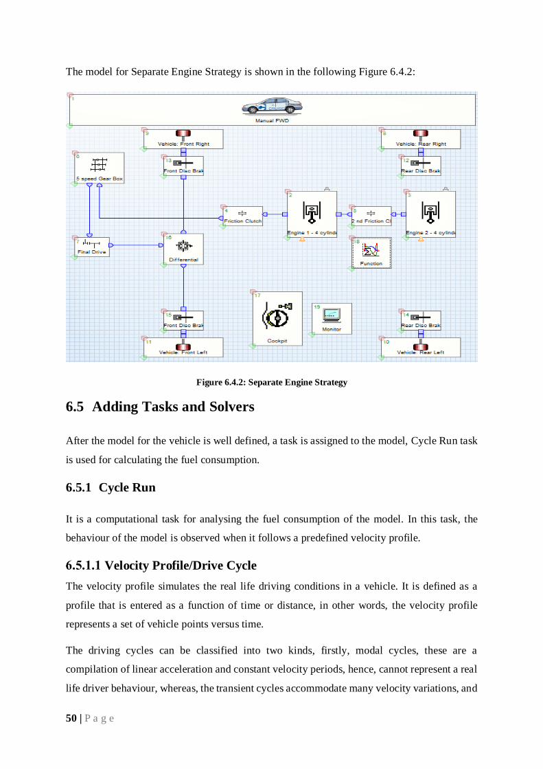
50 | P a g e

The model for Separate Engine Strategy is shown in the following Figure 6.4.2:

Figure 6.4.2: Separate Engine Strategy

6.5 Adding Tasks and Solvers

After the model for the vehicle is well defined, a task is assigned to the model, Cycle Run task

is used for calculating the fuel consumption.

6.5.1 Cycle Run

It is a computational task for analysing the fuel consumption of the model. In this task, the

behaviour of the model is observed when it follows a predefined velocity profile.

Velocity Profile/Drive Cycle

The velocity profile simulates the real life driving conditions in a vehicle. It is defined as a

profile that is entered as a function of time or distance, in other words, the velocity profile

represents a set of vehicle points versus time.

The driving cycles can be classified into two kinds, firstly, modal cycles, these are a

compilation of linear acceleration and constant velocity periods, hence, cannot represent a real

life driver behaviour, whereas, the transient cycles accommodate many velocity variations, and

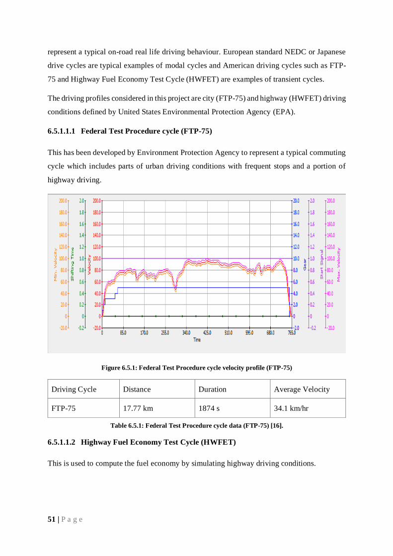
51 | P a g e

represent a typical on-road real life driving behaviour. European standard NEDC or Japanese

drive cycles are typical examples of modal cycles and American driving cycles such as FTP-

75 and Highway Fuel Economy Test Cycle (HWFET) are examples of transient cycles.

The driving profiles considered in this project are city (FTP-75) and highway (HWFET) driving

conditions defined by United States Environmental Protection Agency (EPA).

6.5.1.1.1 Federal Test Procedure cycle (FTP-75)

This has been developed by Environment Protection Agency to represent a typical commuting

cycle which includes parts of urban driving conditions with frequent stops and a portion of

highway driving.

Figure 6.5.1: Federal Test Procedure cycle velocity profile (FTP-75)

Driving Cycle Distance Duration Average Velocity

FTP-75 17.77 km 1874 s 34.1 km/hr

Table 6.5.1: Federal Test Procedure cycle data (FTP-75) [16].

6.5.1.1.2 Highway Fuel Economy Test Cycle (HWFET)

This is used to compute the fuel economy by simulating highway driving conditions.

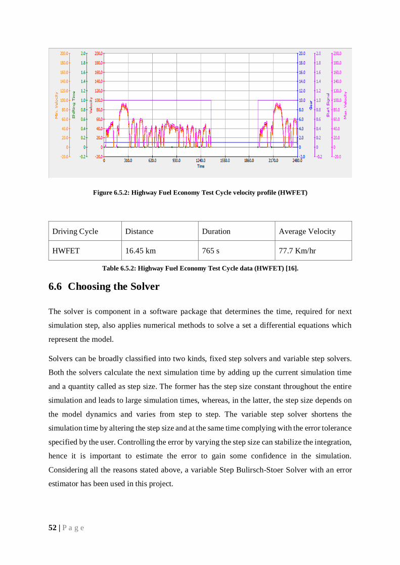
52 | P a g e

Figure 6.5.2: Highway Fuel Economy Test Cycle velocity profile (HWFET)

Driving Cycle Distance Duration Average Velocity

HWFET 16.45 km 765 s 77.7 Km/hr

Table 6.5.2: Highway Fuel Economy Test Cycle data (HWFET) [16].

6.6 Choosing the Solver

The solver is component in a software package that determines the time, required for next

simulation step, also applies numerical methods to solve a set a differential equations which

represent the model.

Solvers can be broadly classified into two kinds, fixed step solvers and variable step solvers.

Both the solvers calculate the next simulation time by adding up the current simulation time

and a quantity called as step size. The former has the step size constant throughout the entire

simulation and leads to large simulation times, whereas, in the latter, the step size depends on

the model dynamics and varies from step to step. The variable step solver shortens the

simulation time by altering the step size and at the same time complying with the error tolerance

specified by the user. Controlling the error by varying the step size can stabilize the integration,

hence it is important to estimate the error to gain some confidence in the simulation.

Considering all the reasons stated above, a variable Step Bulirsch-Stoer Solver with an error

estimator has been used in this project.

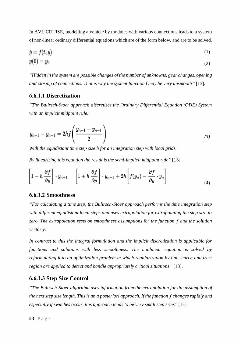
53 | P a g e

In AVL CRUISE, modelling a vehicle by modules with various connections leads to a system

of non-linear ordinary differential equations which are of the form below, and are to be solved.

(1)

(2)

“Hidden in the system are possible changes of the number of unknowns, gear changes, opening

and closing of connections. That is why the system function f may be very unsmooth” [13].

Discretization

“The Bulirsch-Stoer approach discretizes the Ordinary Differential Equation (ODE) System

with an implicit midpoint rule:

(3)

With the equidistant time step size h for an integration step with local grids.

By linearizing this equation the result is the semi-implicit midpoint rule” [13].

(4)

Smoothness

“For calculating a time step, the Bulirsch-Stoer approach performs the time integration step

with different equidistant local steps and uses extrapolation for extrapolating the step size to

zero. The extrapolation rests on smoothness assumptions for the function ƒ and the solution

vector y.

In contrast to this the integral formulation and the implicit discretization is applicable for

functions and solutions with less smoothness. The nonlinear equation is solved by

reformulating it to an optimization problem in which regularization by line search and trust

region are applied to detect and handle appropriately critical situations” [13].

Step Size Control

“The Bulirsch-Stoer algorithm uses information from the extrapolation for the assumption of

the next step size length. This is an a posteriori approach. If the function ƒ changes rapidly and

especially if switches occur, this approach tends to be very small step sizes” [13].

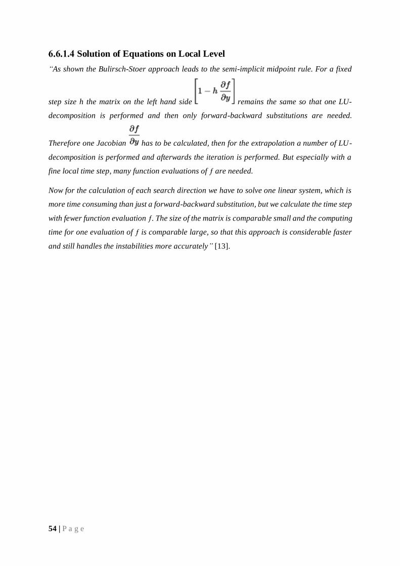
54 | P a g e

Solution of Equations on Local Level

“As shown the Bulirsch-Stoer approach leads to the semi-implicit midpoint rule. For a fixed

step size h the matrix on the left hand side remains the same so that one LU-

decomposition is performed and then only forward-backward substitutions are needed.

Therefore one Jacobian has to be calculated, then for the extrapolation a number of LU-

decomposition is performed and afterwards the iteration is performed. But especially with a

fine local time step, many function evaluations of ƒ are needed.

Now for the calculation of each search direction we have to solve one linear system, which is

more time consuming than just a forward-backward substitution, but we calculate the time step

with fewer function evaluation ƒ. The size of the matrix is comparable small and the computing

time for one evaluation of ƒ is comparable large, so that this approach is considerable faster

and still handles the instabilities more accurately” [13].

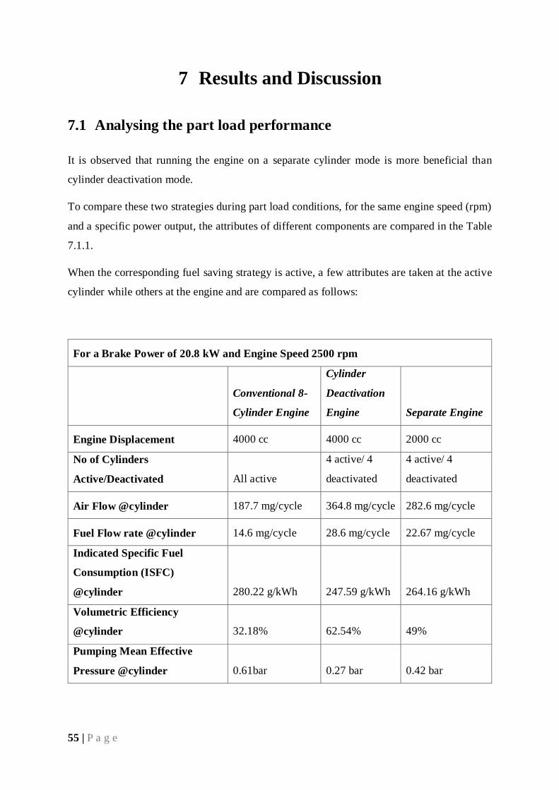
55 | P a g e

7 Results and Discussion

7.1 Analysing the part load performance

It is observed that running the engine on a separate cylinder mode is more beneficial than

cylinder deactivation mode.

To compare these two strategies during part load conditions, for the same engine speed (rpm)

and a specific power output, the attributes of different components are compared in the Table

7.1.1.

When the corresponding fuel saving strategy is active, a few attributes are taken at the active

cylinder while others at the engine and are compared as follows:

For a Brake Power of 20.8 kW and Engine Speed 2500 rpm

Conventional 8-

Cylinder Engine

Cylinder

Deactivation

Engine Separate Engine

Engine Displacement 4000 cc 4000 cc 2000 cc

No of Cylinders

Active/Deactivated All active

4 active/ 4

deactivated

4 active/ 4

deactivated

Air Flow @cylinder 187.7 mg/cycle 364.8 mg/cycle 282.6 mg/cycle

Fuel Flow rate @cylinder 14.6 mg/cycle 28.6 mg/cycle 22.67 mg/cycle

Indicated Specific Fuel

Consumption (ISFC)

@cylinder 280.22 g/kWh 247.59 g/kWh 264.16 g/kWh

Volumetric Efficiency

@cylinder 32.18% 62.54% 49%

Pumping Mean Effective

Pressure @cylinder 0.61bar 0.27 bar 0.42 bar

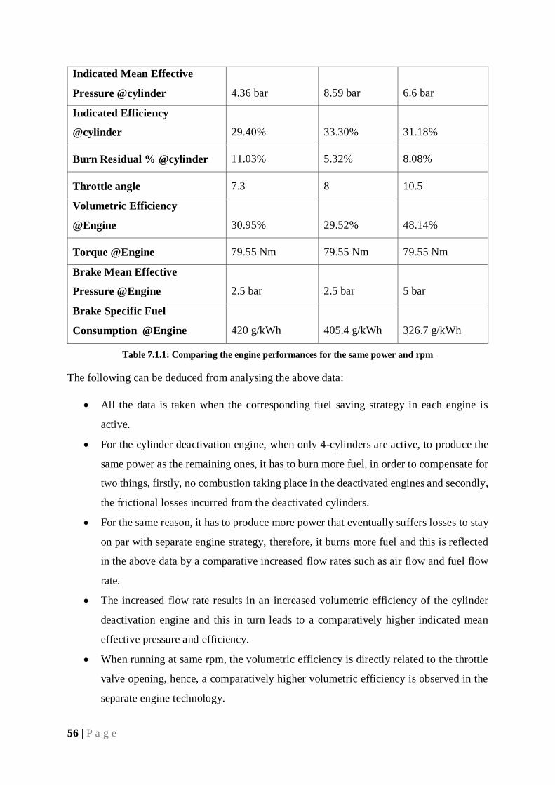
56 | P a g e

Indicated Mean Effective

Pressure @cylinder 4.36 bar 8.59 bar 6.6 bar

Indicated Efficiency

@cylinder 29.40% 33.30% 31.18%

Burn Residual % @cylinder 11.03% 5.32% 8.08%

Throttle angle 7.3 8 10.5

Volumetric Efficiency

@Engine 30.95% 29.52% 48.14%

Torque @Engine 79.55 Nm 79.55 Nm 79.55 Nm

Brake Mean Effective

Pressure @Engine 2.5 bar 2.5 bar 5 bar

Brake Specific Fuel

Consumption @Engine 420 g/kWh 405.4 g/kWh 326.7 g/kWh

Table 7.1.1: Comparing the engine performances for the same power and rpm

The following can be deduced from analysing the above data:

All the data is taken when the corresponding fuel saving strategy in each engine is

active.

For the cylinder deactivation engine, when only 4-cylinders are active, to produce the

same power as the remaining ones, it has to burn more fuel, in order to compensate for

two things, firstly, no combustion taking place in the deactivated engines and secondly,

the frictional losses incurred from the deactivated cylinders.

For the same reason, it has to produce more power that eventually suffers losses to stay

on par with separate engine strategy, therefore, it burns more fuel and this is reflected

in the above data by a comparative increased flow rates such as air flow and fuel flow

rate.

The increased flow rate results in an increased volumetric efficiency of the cylinder

deactivation engine and this in turn leads to a comparatively higher indicated mean

effective pressure and efficiency.

When running at same rpm, the volumetric efficiency is directly related to the throttle

valve opening, hence, a comparatively higher volumetric efficiency is observed in the

separate engine technology.

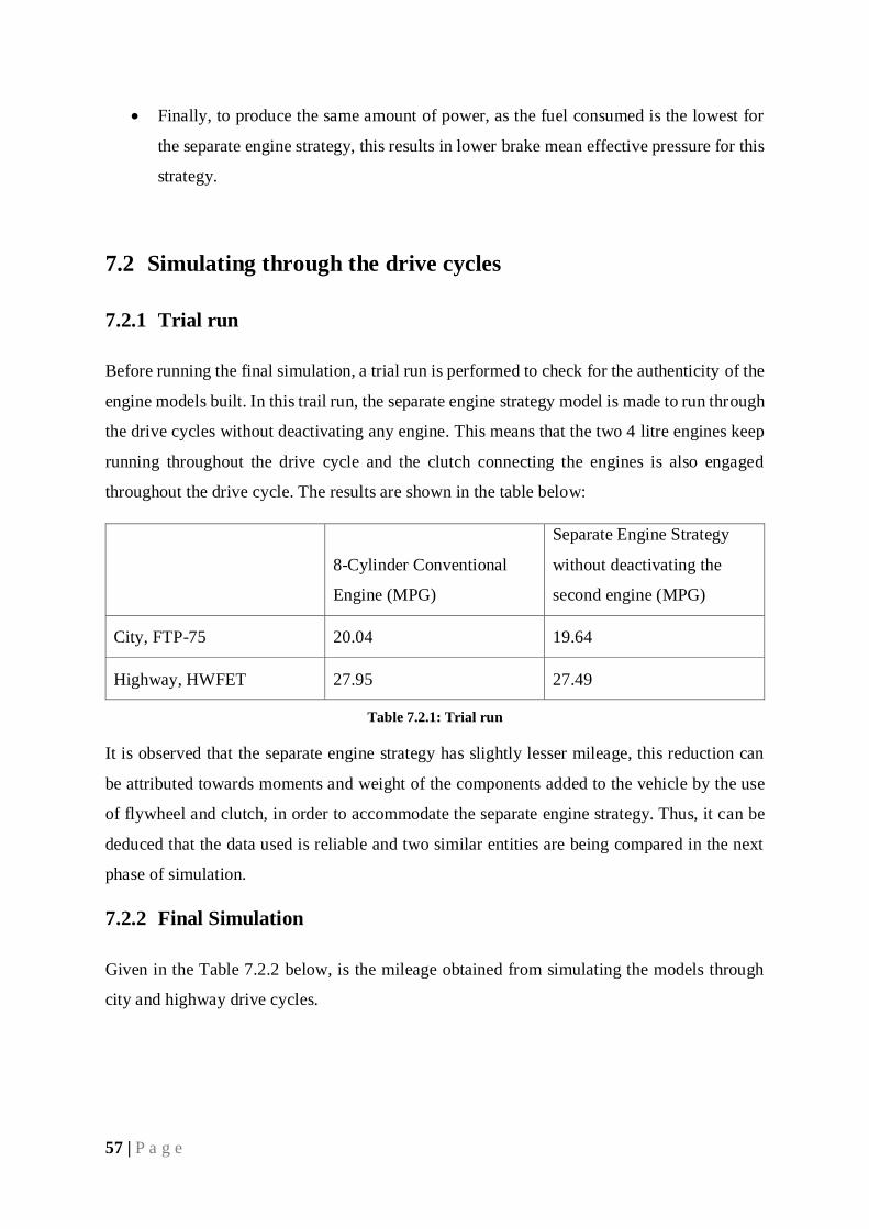
57 | P a g e

Finally, to produce the same amount of power, as the fuel consumed is the lowest for

the separate engine strategy, this results in lower brake mean effective pressure for this

strategy.

7.2 Simulating through the drive cycles

7.2.1 Trial run

Before running the final simulation, a trial run is performed to check for the authenticity of the

engine models built. In this trail run, the separate engine strategy model is made to run through

the drive cycles without deactivating any engine. This means that the two 4 litre engines keep

running throughout the drive cycle and the clutch connecting the engines is also engaged

throughout the drive cycle. The results are shown in the table below:

8-Cylinder Conventional

Engine (MPG)

Separate Engine Strategy

without deactivating the

second engine (MPG)

City, FTP-75 20.04 19.64

Highway, HWFET 27.95 27.49

Table 7.2.1: Trial run

It is observed that the separate engine strategy has slightly lesser mileage, this reduction can

be attributed towards moments and weight of the components added to the vehicle by the use

of flywheel and clutch, in order to accommodate the separate engine strategy. Thus, it can be

deduced that the data used is reliable and two similar entities are being compared in the next

phase of simulation.

7.2.2 Final Simulation

Given in the Table 7.2.2 below, is the mileage obtained from simulating the models through

city and highway drive cycles.

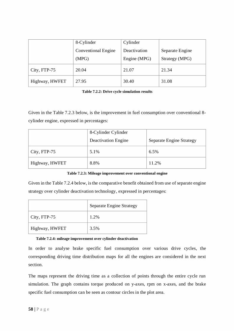
58 | P a g e

8-Cylinder

Conventional Engine

(MPG)

Cylinder

Deactivation

Engine (MPG)

Separate Engine

Strategy (MPG)

City, FTP-75 20.04 21.07 21.34

Highway, HWFET 27.95 30.40 31.08

Table 7.2.2: Drive cycle simulation results

Given in the Table 7.2.3 below, is the improvement in fuel consumption over conventional 8-

cylinder engine, expressed in percentages:

8-Cylinder Cylinder

Deactivation Engine Separate Engine Strategy

City, FTP-75 5.1% 6.5%

Highway, HWFET 8.8% 11.2%

Table 7.2.3: Mileage improvement over conventional engine

Given in the Table 7.2.4 below, is the comparative benefit obtained from use of separate engine

strategy over cylinder deactivation technology, expressed in percentages:

Separate Engine Strategy

City, FTP-75 1.2%

Highway, HWFET 3.5%

Table 7.2.4: mileage improvement over cylinder deactivation

In order to analyse brake specific fuel consumption over various drive cycles, the

corresponding driving time distribution maps for all the engines are considered in the next

section.

The maps represent the driving time as a collection of points through the entire cycle run

simulation. The graph contains torque produced on y-axes, rpm on x-axes, and the brake

specific fuel consumption can be seen as contour circles in the plot area.

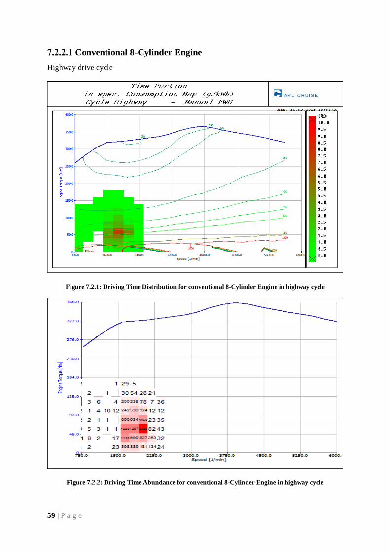
59 | P a g e

Conventional 8-Cylinder Engine

Highway drive cycle

Figure 7.2.1: Driving Time Distribution for conventional 8-Cylinder Engine in highway cycle

Figure 7.2.2: Driving Time Abundance for conventional 8-Cylinder Engine in highway cycle

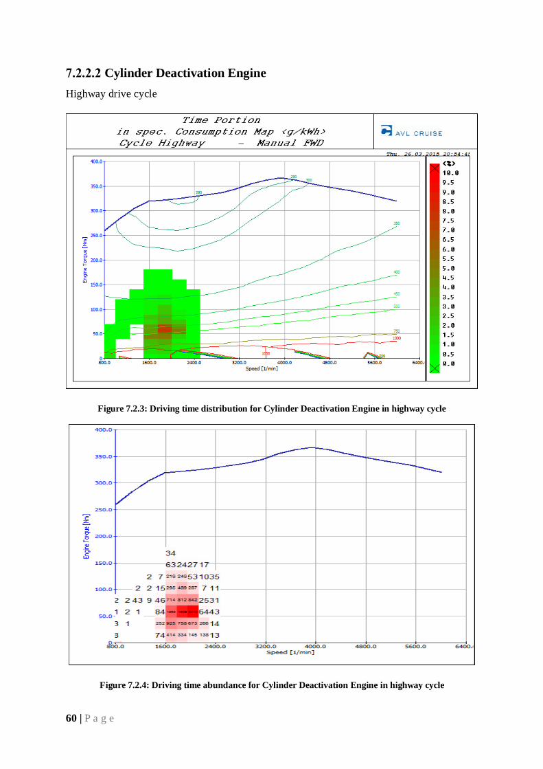
60 | P a g e

Cylinder Deactivation Engine

Highway drive cycle

Figure 7.2.3: Driving time distribution for Cylinder Deactivation Engine in highway cycle

Figure 7.2.4: Driving time abundance for Cylinder Deactivation Engine in highway cycle

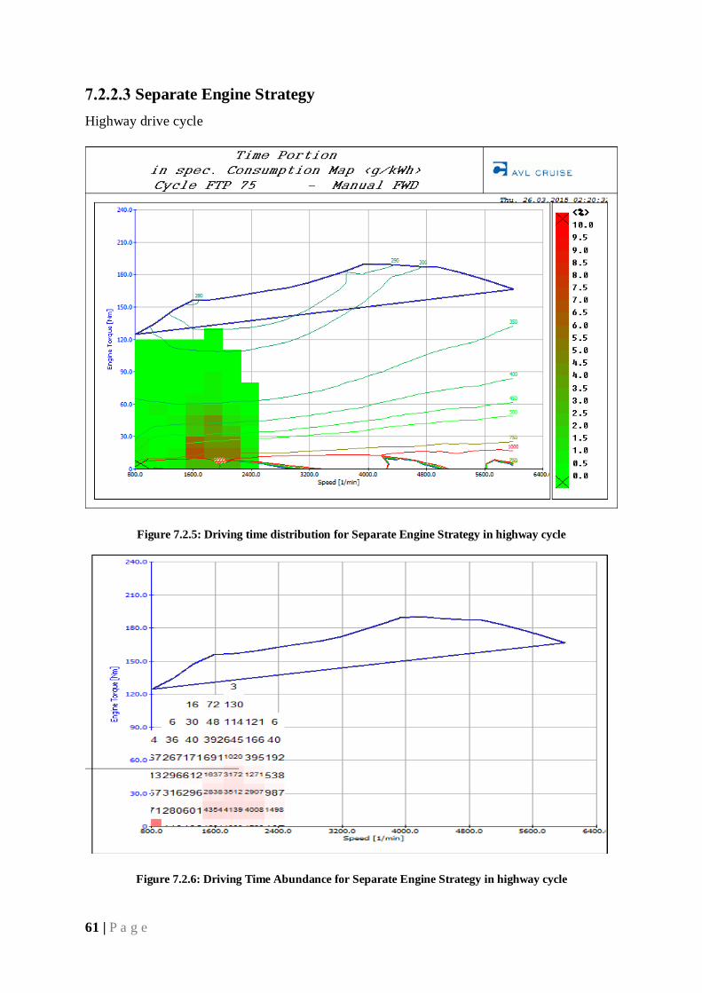
61 | P a g e

Separate Engine Strategy

Highway drive cycle

Figure 7.2.5: Driving time distribution for Separate Engine Strategy in highway cycle

Figure 7.2.6: Driving Time Abundance for Separate Engine Strategy in highway cycle

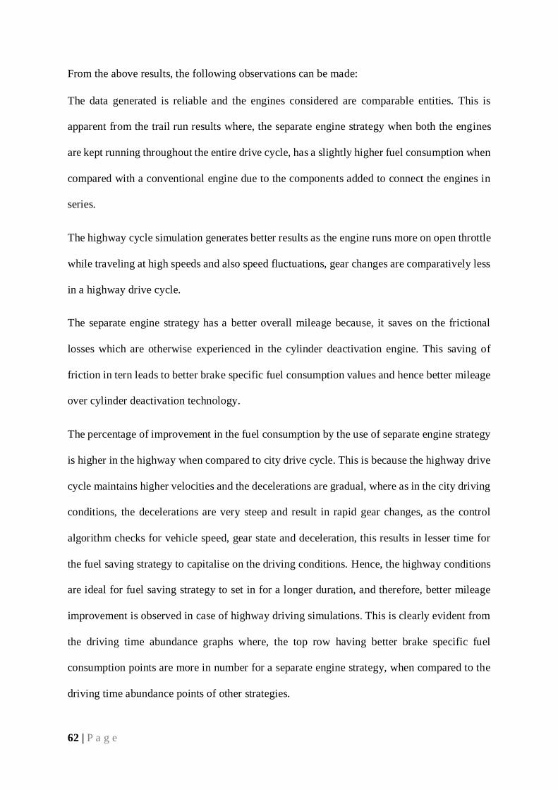
62 | P a g e

From the above results, the following observations can be made:

The data generated is reliable and the engines considered are comparable entities. This is

apparent from the trail run results where, the separate engine strategy when both the engines

are kept running throughout the entire drive cycle, has a slightly higher fuel consumption when

compared with a conventional engine due to the components added to connect the engines in

series.

The highway cycle simulation generates better results as the engine runs more on open throttle

while traveling at high speeds and also speed fluctuations, gear changes are comparatively less

in a highway drive cycle.

The separate engine strategy has a better overall mileage because, it saves on the frictional

losses which are otherwise experienced in the cylinder deactivation engine. This saving of

friction in tern leads to better brake specific fuel consumption values and hence better mileage

over cylinder deactivation technology.

The percentage of improvement in the fuel consumption by the use of separate engine strategy

is higher in the highway when compared to city drive cycle. This is because the highway drive

cycle maintains higher velocities and the decelerations are gradual, where as in the city driving

conditions, the decelerations are very steep and result in rapid gear changes, as the control

algorithm checks for vehicle speed, gear state and deceleration, this results in lesser time for

the fuel saving strategy to capitalise on the driving conditions. Hence, the highway conditions

are ideal for fuel saving strategy to set in for a longer duration, and therefore, better mileage

improvement is observed in case of highway driving simulations. This is clearly evident from

the driving time abundance graphs where, the top row having better brake specific fuel

consumption points are more in number for a separate engine strategy, when compared to the

driving time abundance points of other strategies.

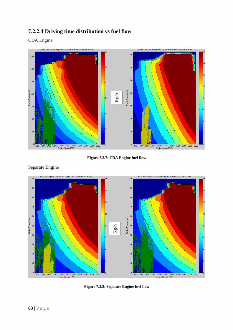
63 | P a g e

Driving time distribution vs fuel flow

CDA Engine

Figure 7.2.7: CDA Engine fuel flow

Separate Engine

Figure 7.2.8: Separate Engine fuel flow

Kg

/h

r

Kg

/h

r

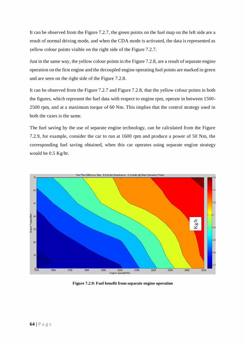
64 | P a g e

It can be observed from the Figure 7.2.7, the green points on the fuel map on the left side are a

result of normal driving mode, and when the CDA mode is activated, the data is represented as

yellow colour points visible on the right side of the Figure 7.2.7.

Just in the same way, the yellow colour points in the Figure 7.2.8, are a result of separate engine

operation on the first engine and the decoupled engine operating fuel points are marked in green

and are seen on the right side of the Figure 7.2.8.

It can be observed from the Figure 7.2.7 and Figure 7.2.8, that the yellow colour points in both

the figures, which represent the fuel data with respect to engine rpm, operate in between 1500-

2500 rpm, and at a maximum torque of 60 Nm. This implies that the control strategy used in

both the cases is the same.

The fuel saving by the use of separate engine technology, can be calculated from the Figure

7.2.9, for example, consider the car to run at 1600 rpm and produce a power of 50 Nm, the

corresponding fuel saving obtained, when this car operates using separate engine strategy

would be 0.5 Kg/hr.

Figure 7.2.9: Fuel benefit from separate engine operation

Kg

/h

r

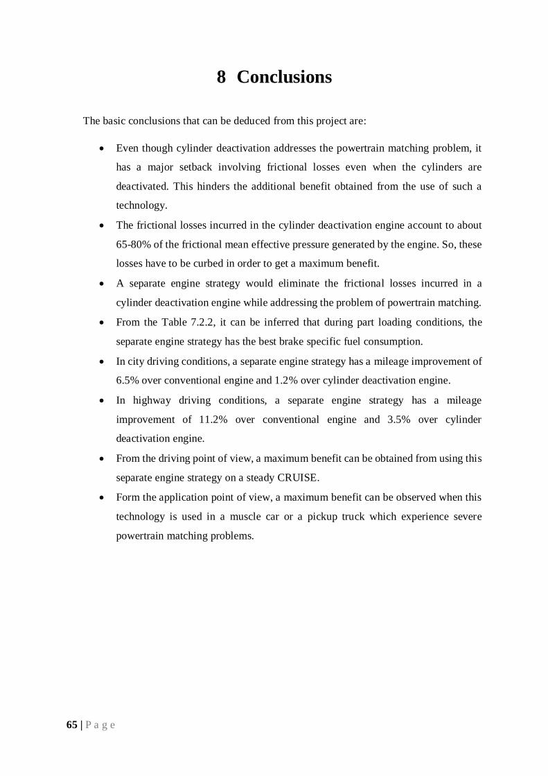
65 | P a g e

8 Conclusions

The basic conclusions that can be deduced from this project are:

Even though cylinder deactivation addresses the powertrain matching problem, it

has a major setback involving frictional losses even when the cylinders are

deactivated. This hinders the additional benefit obtained from the use of such a

technology.

The frictional losses incurred in the cylinder deactivation engine account to about

65-80% of the frictional mean effective pressure generated by the engine. So, these

losses have to be curbed in order to get a maximum benefit.

A separate engine strategy would eliminate the frictional losses incurred in a

cylinder deactivation engine while addressing the problem of powertrain matching.

From the Table 7.2.2, it can be inferred that during part loading conditions, the

separate engine strategy has the best brake specific fuel consumption.

In city driving conditions, a separate engine strategy has a mileage improvement of

6.5% over conventional engine and 1.2% over cylinder deactivation engine.

In highway driving conditions, a separate engine strategy has a mileage

improvement of 11.2% over conventional engine and 3.5% over cylinder

deactivation engine.

From the driving point of view, a maximum benefit can be obtained from using this

separate engine strategy on a steady CRUISE.

Form the application point of view, a maximum benefit can be observed when this

technology is used in a muscle car or a pickup truck which experience severe

powertrain matching problems.

66 | P a g e

9 Future Work

In a separate engine strategy, the second engine turns off when the vehicle complies with a set

of conditions defined. A major limiting condition is the activation of such a technology only

during deceleration, both engines keep running all the time, only when the vehicle decelerates

and other set of conditions are satisfied, the second engine turns off.

Instead of turn off the second engine intermittently, It would be interesting to check for the

feasibly of turning on the engine intermittently. So, an extension of this project would be to

investigate the feasibility of supplying power only on demand. The first engine keeps running

throughout the entire drive cycle, the second engine only kicks-in when there is an additional

power demand form the driver.

There has to be no difference in terms of acceleration in a vehicle having this proposed

technology and a conventional vehicle. For the same gas pedal positions, both these vehicles

have to accelerate in the same way. In order to accomplish this, a continuously variable

transmission has to be used in the vehicle which runs using this proposed technology. The gear

ratios have to be varied depending on how many engines are being used at that particular

instance.

While running on a smaller engine, varying the gear ratios on the continuously variable

transmission and running engine on higher rpms, meets the acceleration demands of the driver.

This allows the first engine to run as close as possible to the optimum operating line and thus,

the efficiency gets improved.

67 | P a g e

References

[1] Fukui, T., T. Nakagami, H. Endo, T. Katsumoto, and Y. Danno, “Mitsubishi Orion-

MD – A New Variable Displacement Engine”, SAE Paper 831007, 1983.

[2] T.G. Leone and M Pozar “Fuel Economy Benefit of Cylinder Deactivation –

Sensitivity to Vehicle Application and Operating Constraints”, SAE Paper 2001-01-

3591

[3] Quan Zheng, “Characterization of the Dynamic Response of a Cylinder Deactivation

Valvetrain System”, SAE Paper 2001-01-0669

[4] Falkowski, A., McElwee, M., and Bonne, M., “Design and Development of the

DaimlerChrysler 5.7L HEMI® Engine Multi-Displacement Cylinder Deactivation

System,” SAE Technical Paper 2004-01-2106

[5] Vinodh, B., “Technology for Cylinder Deactivation,” SAE Technical Paper 2005-01-

0077

[6] Fujiwara, M., Kumagai, K., Segawa, M., Sato, R. et al., “Development of a 6-Cylinder

Gasoline Engine with New Variable Cylinder Management Technology,”SAE

Technical Paper 2008-01-0610

[7] Boretti, A. and Scalco, J., “Piston and Valve Deactivation for Improved Part Load

Performances of Internal Combustion Engines,” SAE Technical Paper 2011-01-0368

[8] Bates, B., J. M. Dosdall, and D. H. Smith, "Variable Displacement by Engine Valve

Control", SAE Paper 780145, 1978

[9] “http://www.free-vectors.com/images/Transport/027-free-sports-car-vector-clip-art-

l.png,”[Online]

[10] "Part Load Pumping Losses in an SI Engine." Part Load Pumping Losses In A Spark

Ignited IC Engine. N.p., n.d. Web. 28 Mar. 2015.

68 | P a g e

[11] M. Wilcutts, J. Switkes, M. Shost, and A. Tripathi, “Design and Benefits of Dynamic

Skip Fire Strategies for Cylinder Deactivated Engines,” SAE Int. J. Engines, vol. 6,

pp. 278–288, 2013.

[12] “http://www.csa.com/discoveryguides/auto/review4.php,”[online]

[13] AVL, AVL CRUISE: User Guide, 2014.

[14] AVL, AVL BOOST: User Guide, 2013.

[15] "Ford Clutch-Flywheel Assemblies - Tilton Engineering." Tilton Engineering. N.p.,

n.d. Web. 29 Mar. 2015. <http://tiltonracing.com/product/ford-clutch-flywheel-

assemblies/>

[16] "The Different Driving Cycles." Car Engineer. N.p., 05 Jan. 2013. Web. 20 Nov. 2014.

<http://www.car-engineer.com/the-different-driving-cycles/>.

[17] "The BSFC Chart Thread (post 'em If You Got 'em) - Page 12 - Fuel Economy,

Hypermiling, EcoModding News and Forum - EcoModder.com." EcoModdercom

RSS. N.p., n.d. Web. 06 May 2015.

<http://ecomodder.com/forum/showthread.php/bsfc-chart-thread-post-em-if-you-

got-1466-12.html>

[18] K. Douglas, N. Milovanovic, J. Turner, and D. Blundell, “Fuel Economy

Improvement Using Combined CAI and Cylinder Deactivation (CDA)-An Initial

Study,” Sae Tech. Pap. Ser. 2005-01-0110, vol. 2005, no. 724, 2005.

[19] M. Farid, M. Said, A. Bin, A. Aziz, Z. A. Latiff, and A. M. Andwari, “Investigation

of Cylinder Deactivation ( CDA ) Strategies on Part Load Conditions,” 2014.

[20] M. Rebbert, G. Kreusen, and S. Lauer, “A New Cylinder Deactivation by FEV and

Mahle,” Sae Sp, vol. 2174, no. 724, p. 105, 2008.

[21] E. Watanabe and I. Fukutani, “The Engineering Resource For Advancing Mobility

Cylinder Cutoff of 4-Stroke Cycle Engines at Part-Load and idle,” 1982.

69 | P a g e

[22] K. Douglas, N. Milovanovic, J. Turner, and D. Blundell, “Fuel Economy

Improvement Using Combined CAI and Cylinder Deactivation (CDA)-An Initial

Study,” Sae Tech. Pap. Ser. 2005-01-0110, vol. 2005, no. 724, 2005.

[23] M. Farid, M. Said, A. Bin, A. Aziz, Z. A. Latiff, and A. M. Andwari, “Investigation

of Cylinder Deactivation ( CDA ) Strategies on Part Load Conditions,” 2014.

[24] "Pics For Car Clutch Animation." Pics For Car Clutch Animation. N.p., n.d. Web. 30

Jan. 2015. <http://pixshark.com/car-clutch-animation.htm>

70 | P a g e

VITA AUCTORIS

NAME: Shravan Kumar Sadhu

PLACE OF BIRTH:

Vuyyuru, AP, India

YEAR OF BIRTH:

1989

EDUCATION:

Johnson Grammar School, Hyderabad, AP, 2005

MVSR Engg. College, Hyderabad, AP, 2011

University of Windsor, M.Sc., Windsor, ON, 2015