Embed Size (px)
Citation preview
Institut für Linguistik – Phonetik Universität zu Köln
Investigating potential acoustic correlates of sonority:
Intensity vs. periodic energy
Bachelorarbeit an der Philosophischen Fakultät der Universität zu Köln
im Fach Linguistik und Phonetik
vorgelegt von
Tobias Reinhold Schröer
Köln, 10.08.2020
Prüferin: Prof. Dr. Martine Grice
i
Table of Contents
1 Introduction..............................................................................................................1
2 Overview of sonority...............................................................................................1
2.1 Background......................................................................................................2
2.2 Why acoustics?.................................................................................................5
3 Study........................................................................................................................7
3.1 Method.............................................................................................................8
3.1.1 Experimental setup...................................................................................8
3.1.2 Measurements...........................................................................................8
3.1.2.1 Peaks...............................................................................................12
3.1.2.2 Summing and averaging.................................................................14
3.1.3 Statistical calculation..............................................................................15
3.2 Results............................................................................................................16
3.3 Analysis..........................................................................................................20
3.3.1 Peaks.......................................................................................................21
3.3.1.1 Minima............................................................................................21
3.3.1.2 Maxima...........................................................................................24
3.3.2 Sum.........................................................................................................27
3.3.3 Average...................................................................................................30
3.4 Discussion......................................................................................................33
3.4.1 The role of duration: Summing makes a difference...............................33
3.4.2 The role of segmentation: Why min is better than max.........................35
3.4.3 The mean between: The robustness of the average measure..................36
3.4.4 General remarks......................................................................................37
4 Conclusion.............................................................................................................38
References...................................................................................................................40
1
1 Introduction
Spoken language consists of speech sounds that combine into syllables, and fur-
ther on, into words and phrases. Within syllables, speech sounds cannot be combined
completely arbitrarily. For example, the sequence /plid/ is considered a syllable in,
e.g., the English language, but /lpid/ is not. In order to describe what sounds can be
combined in which way, the concept of sonority is consulted. Generally speaking,
sounds with a high sonority (mostly vowels) form the nucleus, i.e. the centre, of a
syllable. They can (but do not have to) be surrounded by other sounds (mostly con-
sonants) with a lower sonority than the nucleus. From the syllable onset, i.e. its be-
ginning, to its nucleus, sonority is expected to rise. Conversely, from nucleus to coda,
i.e. the syllable’s end, sonority is expected to fall. Regarding the example above, /l/ is
considered more sonorous than /p/, which is why /plid/ forms a syllable, in contrast
to /lpid/. The same applies to codas: /hɛlp/ is considered a syllable, whereas /hɛpl/ is
not.
The assignment of sonority ranks to speech sounds primarily grounds on linguistic
observations on how speech sounds can be combined in different languages. Still,
there is no agreement on whether sonority has a physical, measurable basis. Some re-
searchers even deny the concept of sonority entirely. In this thesis, I aim at contribut-
ing to the discussion by exploring possible acoustic correlates of sonority. To do so, I
will first give an overview of the research on sonority (section 2). Following, I will
report on an exploratory pilot study I conducted, describing and discussing the acous-
tic measurements in detail (section 3). In section 4, the thesis finishes with a conclu-
sion and an outlook on further research.
The data and the code from this study can be found at https://osf.io/w5cje/?
view_only=f3b7aa80fcc940aba83ddf21512efe5c.
2 Overview of sonority
This section gives an overview on the subject of sonority. First, the scientific
background is presented (subsection 2.1). Subsequently, I explain my decision to ex-
plore possible sonority correlates in the acoustic domain, taking into account recent
findings (subsection 2.2).
2
2.1 Background
The discussion on the topic of sonority as a core principle behind syllables has
quite a long history in linguistics, with Sievers (1893/1901) being the first to intro-
duce it by the term Schallfülle (‘sound fullness’). He states that every speech sound
has a certain sonority value and that within a syllable, the sounds with a relatively
low sonority (which Sievers links to loudness) mark its boundaries, and, in turn, very
sonorous sounds form the syllabic nucleus. According to him, however, there is no
uniform definition of the term ‘syllable’. He describes them as subjective perceptual
segmentations of speech, which are reported to be based on discontinuities in sonor-
ity. Thus, his work can be seen as an early approach to define syllables – an issue
which until today has not been solved.
There has been an ongoing debate about the notion of sonority, regarding its
definition, possible measurable correlates, or its existence altogether. Kawasaki
(1982) sheds light on the missing definition of the idea of sonority. She presents a de-
bate on whether the concept should be explained phonologically or phonetically. She
argues for a phonetic approach, because phonological explanations were prone to cir-
cular reasoning.
Ohala (1992) holds a similar view. He completely rejects the idea of sonority due
to a missing measurable correlate and the thereby inherent circularity in its defini-
tion: In his view, sonority only describes the preferable ordering of sounds in a syl-
lable, which remains hard to define with any consistent criterion. Since the prefer-
ence for some speech sound combinations cannot be accounted for by the sonority
hierarchy and some relatively prevalent consonant clusters (such as /st-/ or /-kʃ/)
even violate the hierarchy, he suggests to directly consult the physical parameters
amplitude, periodicity, spectral shape and fundamental frequency (F0), ‘which are
well known and readily measured in the speech signal’ (Ohala 1992: 325).
Clements (1990) argues that the fact that there is no physical definition for a
concept does not make it useless for research. This was true for sonority as well as
phonemes or syllables. He proposes a number of phonological features (sonorant, ap-
proximant, vocoid, syllabic) in order to explain the cross-linguistically similar sonor-
ity scales.
3
According to Parker (2011), sonority ‘can be defined as a unique type of relative,
n-ary (non-binary) featurelike phonological element that potentially categorises all
speech sounds into a hierarchical scale’ (Parker 2011: 1160). He states that, as the
classes of sonority are mostly categorised based on manner of articulation, this is the
closest correlate in traditional phonetic terms. This statement, however, is just of de-
scriptive nature and has no explanatory value due to its circularity. Parker (2011)
calls sonority ‘featurelike’ because it can cluster speech segments into several
groups. On the other hand, he describes sonority as being ‘unlike most features’ be-
cause without exception every segment bears a certain value of it. In a meta-study
(Parker 2017), he analyses 264 studies dealing with sonority by one means or an-
other, with approx. 57 % of them indicating a significant role of sonority for explain-
ing the results, even MRI analyses of brain functions.
In response to the points of criticism regarding the phonetic substance of sonority
(Kawasaki 1982; Ohala 1992), Parker (2008) conducts a study investigating the cor-
relation between sonority (more precisely, his scale given in (2)) and intensity, which
results in a mean Spearman’s correlation of 0.91. In contrast, Albert and Nicenboim
(2020) argue that sonority refers to pitch intelligibility: Vowels are the most sonorous
speech sounds and can best convey pitch. In contrast, a voiceless obstruent is not a
good carrier of pitch information, due to its minimal amount of periodic energy. So,
pitch intelligibility in turn correlates with periodic energy, a subpart of the overall in-
tensity of the acoustic signal (Albert et al. 2018).
Another issue concerning sonority is that a number of different scales have been
proposed. Parker (2002), e.g., reports on over 100 sonority hierarchies of which some
are language-specific and others claim to be cross-linguistically applicable. In this
study, I will consult three sonority scales of which one scale, put forward inter alia
by Clements (1990), is often considered the lowest common denominator, see (1).
All sonority hierarchies depicted here start with the most sonorous group of seg-
ments, going down to the least sonorous.
4
(1) Vowels
Glides
Liquids
Nasals
Obstruents
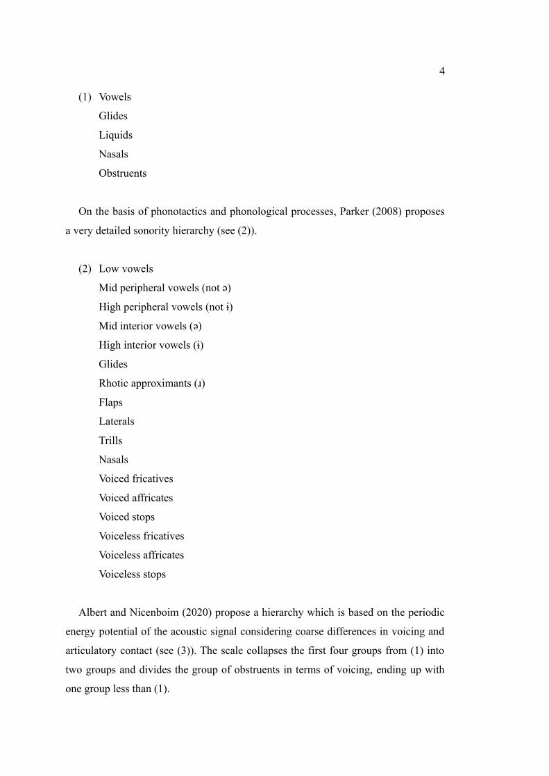
On the basis of phonotactics and phonological processes, Parker (2008) proposes
a very detailed sonority hierarchy (see (2)).
(2) Low vowels
Mid peripheral vowels (not ə)
High peripheral vowels (not ɨ)
Mid interior vowels (ə)
High interior vowels (ɨ)
Glides
Rhotic approximants (ɹ)
Flaps
Laterals
Trills
Nasals
Voiced fricatives
Voiced affricates
Voiced stops
Voiceless fricatives
Voiceless affricates
Voiceless stops
Albert and Nicenboim (2020) propose a hierarchy which is based on the periodic
energy potential of the acoustic signal considering coarse differences in voicing and
articulatory contact (see (3)). The scale collapses the first four groups from (1) into
two groups and divides the group of obstruents in terms of voicing, ending up with
one group less than (1).
5
(3) Sonorant vocoids (e.g. glides, vowels)
Sonorant contoids (e.g. nasals, liquids)
Voiced obstruents (e.g. stops, fricatives)
Voiceless obstruents (e.g. stops, fricatives)
Proceeding from sonority scales, there are various approaches of combinatorial
rules for composing well-formed syllables, among them the Sonority Sequencing
Principle, the Minimum Sonority Distance (Steriade 1982, Selkirk 1984) and the re-
cently proposed Nucleus Attraction Principle (Albert & Nicenboim 2020). However,
as this thesis does not deal with syllabic well-formedness, these principles are not ex-
plained in detail. If the reader is interested in a thorough overview on the literature of
sonority, the publications of Parker (2002; 2017) are recommended.
In summary, there is a considerable amount of evidence that the notion of sonority
can explain phonological concepts such as syllable structure. Yet, as long as there is
no agreement on a phonetic basis for sonority, this explanation remains circular: Son-
ority describes syllable structure, but on the other hand, syllable structure is based on
sonority (and other phonotactic observations). In order to break this circularity, son-
ority has to be defined on an independent, phonetic basis.
2.2 Why acoustics?
In this thesis, I examine acoustic recordings to search for possible measurable cor-
relates of sonority. I will outline this decision in the following. As Ladefoged (1997)
points out, both articulation and perception play an important role in phonetics as
well in phonology, because language only works if it can be produced and under-
stood properly. Acoustics combine both dimensions, as they represent the output of
articulation and the input of perception. Thus, acoustic recordings are a very access-
ible way to examine both of them. Of course, it is a challenge to find out which
acoustic parameter reflects which articulatory or perceptual aspect. In this thesis,
however, I only investigate possible acoustic correlates of sonority without further
discussing their link to articulation or perception.
6
To date, no clear picture has emerged on which parameter suits best as an acoustic
correlate. Parker (2002) measured intensity, F1 frequency and segmental duration for
English and Spanish, in addition to some articulatory dimensions. He concludes that
intensity performs best for both languages, compared to all other acoustic and articu-
latory parameters. He confirms the high correlation of intensity with sonority indices
in a second study for these two languages and, in addition, Cusco Quechua. Jany et
al. (2007), in turn, confirm this finding for Egyptian Arabic, Hindi, Malalayam and
Mongolian, even though some cross-linguistic differences are reported.
Gordon et al. (2012) examine the values of duration, maximum intensity, F1 val-
ues, total acoustic intensity, and total perceptual energy (filtered total acoustic intens-
ity) for five languages (Hindi, Besemah, Armenian, Javanese and Kwak’wala). Their
study is only concerning vowels and aims at finding a measurement that predicts the
low sonority value of schwa. They do not find a value that consistently performs cor-
rectly for all languages and conclude that sonority might be a multi-dimensional vari-
able, which is in line with the findings from Komatsu et al. (2002) for Japanese con-
sonants.
Another reason why acoustics are studied often is the possible enhancement of
speech technology, such as automatic speech recognition (ASR). Kawai and van
Santen (2002), Nakajima et al. (2012) and Patha et al. (2016) go in this direction.
Kawai and van Santen (2002) use the RMS power of filtered frequency bands to dis-
criminate between speech sound classes and in this way detect syllable nuclei. Na-
kajima et al. (2012) follow a similar approach, conducting a factor analysis for
acoustic power. They find that a factor around 1000 Hz correlates best with sonority.
Both studies were conducted with English recordings. Patha et al. (2016) analyse re-
cordings for the languages Telugu, Tamil and Hindi. They band-pass filter the speech
signal between 500 Hz and 1700 Hz and report that the amplitude of the dominant
resonance frequency works best for detecting syllable nuclei and boundaries.
Ladefoged (1997) and Heselwood (1998) suggest to analyse periodic energy for
sonority. Periodic energy forms part of the intensity of the acoustic signal, but is lim-
ited to its (quasi-)periodic portion (Albert et al. 2018). It could serve as a better son-
ority correlate than intensity: For example, the fricative /s/ might have a high intens-
7
ity because of the friction, but still a low sonority value, due to the missing periodic
energy.
There has not been much research on the link between periodic energy and sonor-
ity. Llanos et al. (2015) compare intensity and Shannon entropy for English. Shannon
entropy is akin to detecting periodic energy: a higher periodicity in the signal leads to
a higher Shannon entropy. They report that Shannon entropy is a better correlate for
their proposed hierarchy (vowel > approximant > nasal > fricative > affricate > stop)
than intensity. It is notable that their database consists of 6300 sentences from 630
speakers. Albert and Nicenboim (2020) conduct a syllable count task and conclude
that periodic energy (integrated over time) serves best as foundation for a sonority
model to predict their experiment’s results. Therefore, they propose the periodicity-
based Nucleus Attraction Principle as a new model of sonority.
Due to the given evidence, I view acoustics as a promising chance to explore the
phonetic nature of sonority. In the course of this thesis, I will explore the correlation
between different measurements for intensity and periodic energy and three distinct
sonority scales.
3 Study
In order to investigate possible sonority correlates, I analysed consonants from
acoustic recordings from a pilot experiment conducted at the Institute for Linguistics
– Phonetics, University of Cologne.
For every consonant, I examined various measurements of intensity and periodic
energy so as to cover all main possibilities to measure a continuous curve: minimum
and maximum peaks, sums and averages. By this, I wanted to eliminate the possibil-
ity that the results of this exploratory study are biased due to a specific measuring
technique.
In order to conduct measurements on speech sounds, the audio stream has to be
segmented. However, phones are not produced sequentially, but with a considerable,
variable overlap (e.g. Bell-Berti & Harris 1981, Browman & Goldstein 1992). There-
fore, audio segments are inevitably influenced by the neighbouring segments and
cannot provide for a clear-cut distinction. Nevertheless, for an acoustical analysis of
single speech sounds, a segmentation has to be made based on predefined criteria.
8
These criteria and the experimental setup will be explained in detail in subsection
3.1. Further on, I will report on the results of this exploratory study in subsection 3.2,
followed by a more detailed analysis (subsection 3.3) and the discussion (subsection
3.4).
3.1 Method
In this section, I will outline the setup of the experiment that produced the record-
ings I studied (subsection 3.1.1). After that, I will elaborate on my analysis proced-
ure, concerning the measurements I conducted (subsection 3.1.2) and the statistical
calculation (subsection 3.1.3).
3.1.1 Experimental setup
The experiment was carried out with five participants (1 female, 4 male). Three of
them had German as a native language, one Dutch and one Hebrew. All speakers had
grown up monolingually and were trained phoneticians. Participants were asked to
read out a carrier phrase in their native language with one alternating target pseudo-
word in non-final position. For German, the phrase was ‘Ich möchte […] kaufen’ (‘I
would like to buy […]’). In Dutch, the phrase was ‘Wij kunnen […] kopen’ (‘We can
buy […]’), and for Hebrew, it read ‘כרגע […] רואה ’הוא
(/(h)u ʁo.ˈe […] ka.ˈʁe.ga/ ‘He is seeing […] at the moment’).
The target word had the form of /aˈCa/, an alternating consonant surrounded by
the vowel /a/. Each of the 17 alternating consonants was produced and recorded once
per participant. I limited my study to bilabial, labiodental and alveolar consonants as
well as glides, so four consonants (/k/, /g/, /x/ and /ʃ/) were excluded. For a list of the
13 consonants that went into this study, see Table 1 in subsection 3.1.3.
3.1.2 Measurements
The recordings were edited by extracting the target words from the carrier phrases
and adding a 100 ms padding before and after. Each file was then normalised to a
loudness target of -20 LUFS (Loudness Units relative to Full Scale, ITU-R 2015).
The segmental annotation was done with Praat (Boersma & Weenink 2020), the stat-
istical analysis was carried out using R (R Core Team 2020). The extraction of in-
9
tensity and periodic energy was based on a workflow for Praat and R (Albert et al.
2020), building upon methods from Albert et al. (2018).
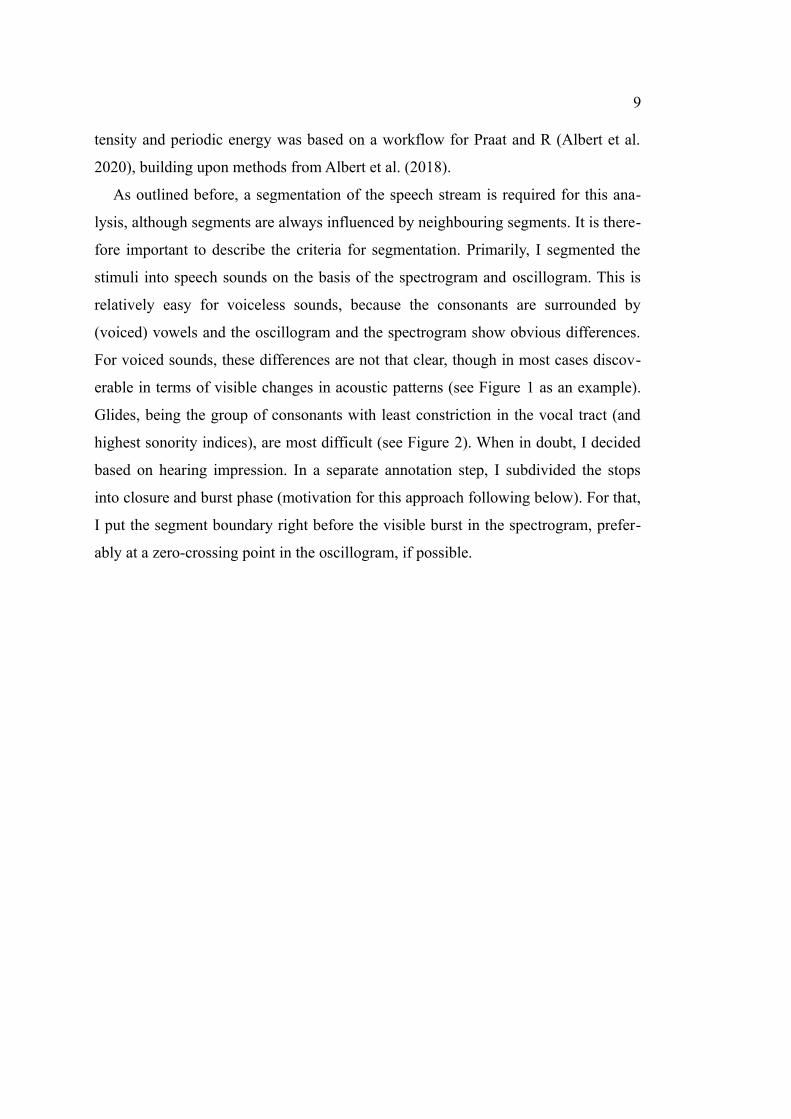
As outlined before, a segmentation of the speech stream is required for this ana-
lysis, although segments are always influenced by neighbouring segments. It is there-
fore important to describe the criteria for segmentation. Primarily, I segmented the
stimuli into speech sounds on the basis of the spectrogram and oscillogram. This is
relatively easy for voiceless sounds, because the consonants are surrounded by
(voiced) vowels and the oscillogram and the spectrogram show obvious differences.
For voiced sounds, these differences are not that clear, though in most cases discov-
erable in terms of visible changes in acoustic patterns (see Figure 1 as an example).
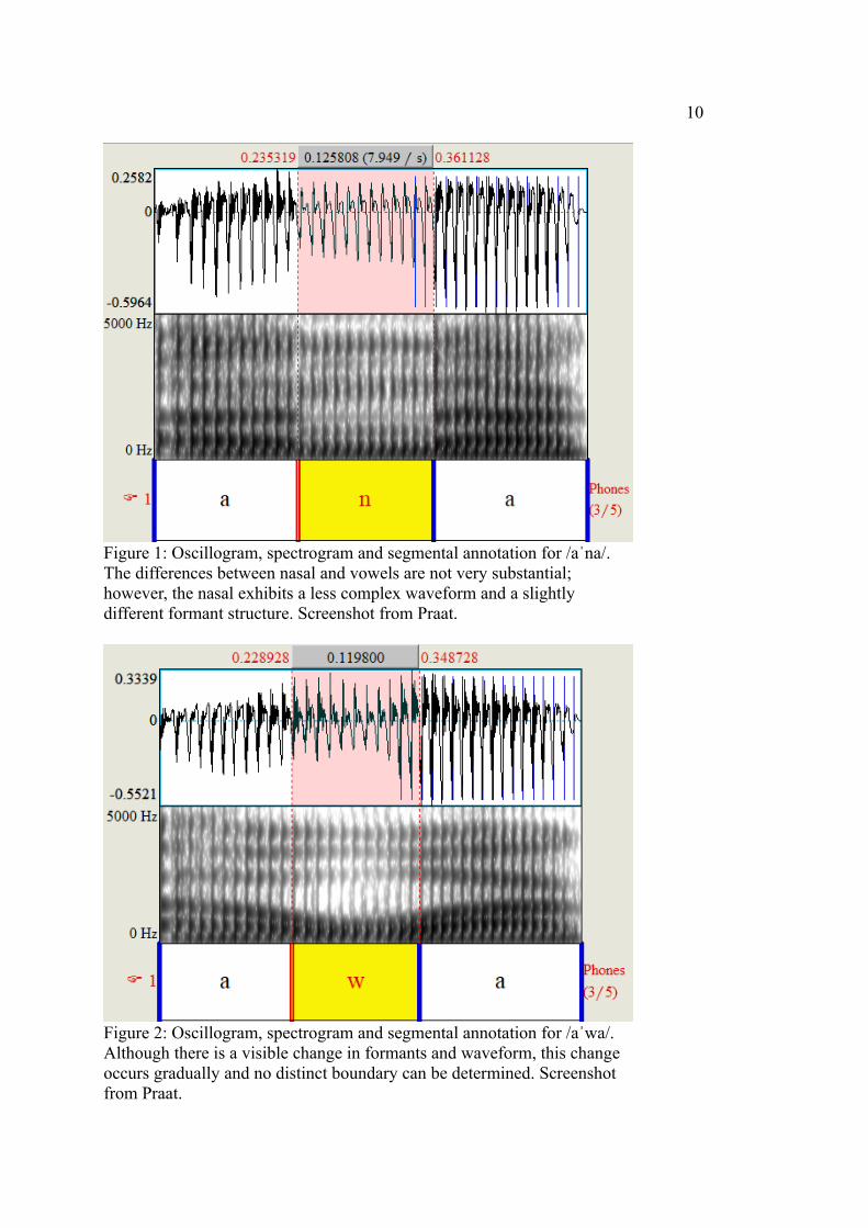
Glides, being the group of consonants with least constriction in the vocal tract (and
highest sonority indices), are most difficult (see Figure 2). When in doubt, I decided
based on hearing impression. In a separate annotation step, I subdivided the stops
into closure and burst phase (motivation for this approach following below). For that,
I put the segment boundary right before the visible burst in the spectrogram, prefer-
ably at a zero-crossing point in the oscillogram, if possible.
10
Figure 1: Oscillogram, spectrogram and segmental annotation for /aˈna/. The differences between nasal and vowels are not very substantial; however, the nasal exhibits a less complex waveform and a slightly different formant structure. Screenshot from Praat.
Figure 2: Oscillogram, spectrogram and segmental annotation for /aˈwa/. Although there is a visible change in formants and waveform, this change occurs gradually and no distinct boundary can be determined. Screenshot from Praat.
11
The variables I analysed are intensity and periodic energy. Intensity refers to the
power of the whole signal, whereas periodic energy is the power of its periodic com-
ponents. It is important to keep in mind that dealing with continuous acoustic meas-
urements means dealing with a curve, rather than discrete values. A curve always
comes with two dimensions – in this case, power and time. There are several valid
measurements that account for these two dimensions: peaks, summing and aver-
aging. I will implement all of them so as to explore which measuring technique suits
best for this study.
Some of the measurements are sensitive to segmentation. In natural language, we
cannot determine one clear point in time where one segment ends and the other be-
gins. However, for studies like this, which link continuous acoustic variables to dis-
crete categorical representations of segments, the segmentation of the audio stream is
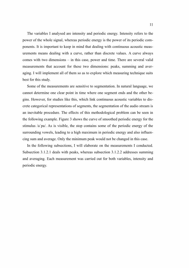
an inevitable procedure. The effects of this methodological problem can be seen in
the following example. Figure 3 shows the curve of smoothed periodic energy for the
stimulus /aˈpa/. As is visible, the stop contains some of the periodic energy of the
surrounding vowels, leading to a high maximum in periodic energy and also influen-
cing sum and average. Only the minimum peak would not be changed in this case.
In the following subsections, I will elaborate on the measurements I conducted.
Subsection 3.1.2.1 deals with peaks, whereas subsection 3.1.2.2 addresses summing
and averaging. Each measurement was carried out for both variables, intensity and
periodic energy.
12
Figure 3: Diagram of the recording /aˈpa/ (x axis: time, y axis: periodic energy) with its segmentation. Because no single segment border can be established naturally, influences by surrounding segments are visible. Althoughbeing a voiceless stop, /p/ contains some periodic energy of the previous and following /a/. Diagram created by means of Praat & R workflow (Albert et al. 2020).
3.1.2.1 Peaks
Peak values are a simple measuring technique: In our case, for a given time win-
dow, the minimum or maximum value of the examined variable (intensity/periodic
energy) is identified. Since this is an exploratory study, I analysed both minimum and
maximum values.
Parker (2008) measured the intensity minimum for consonants and the maximum
for vowels. He justifies this decision by the fact that this would eliminate segmenta-
tion issues, because for consonants, the minimum intensity is likely to occur in the
centre of the audible consonant and not at the boundaries. The same applies to vow-
els and their maximum. This way, the exact segmentation is not important. Apart
from this basic minimum value, Parker (2008) comes up with a special measurement:
Because aspirated stops often exhibit two local minima (one during closure and one
during burst phase), Parker (2008) averages these two minima in such cases. In order
to review this measurement, I set up a scale with simple minima for all sounds except
13
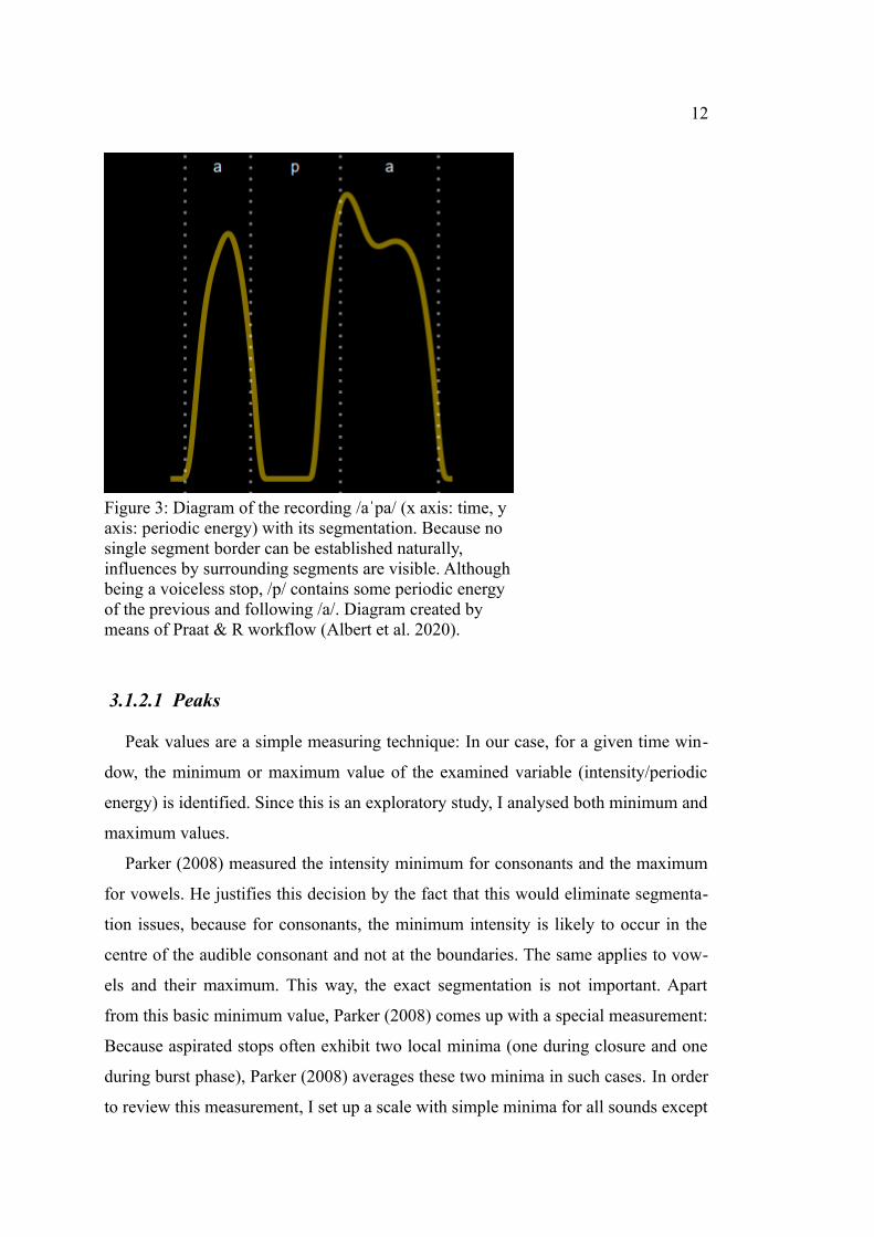
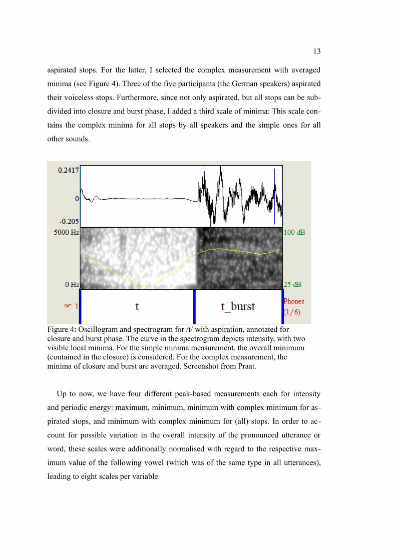
aspirated stops. For the latter, I selected the complex measurement with averaged
minima (see Figure 4). Three of the five participants (the German speakers) aspirated
their voiceless stops. Furthermore, since not only aspirated, but all stops can be sub-
divided into closure and burst phase, I added a third scale of minima: This scale con-
tains the complex minima for all stops by all speakers and the simple ones for all
other sounds.
Figure 4: Oscillogram and spectrogram for /t/ with aspiration, annotated for closure and burst phase. The curve in the spectrogram depicts intensity, with two visible local minima. For the simple minima measurement, the overall minimum (contained in the closure) is considered. For the complex measurement, the minima of closure and burst are averaged. Screenshot from Praat.
Up to now, we have four different peak-based measurements each for intensity
and periodic energy: maximum, minimum, minimum with complex minimum for as-
pirated stops, and minimum with complex minimum for (all) stops. In order to ac-
count for possible variation in the overall intensity of the pronounced utterance or
word, these scales were additionally normalised with regard to the respective max-
imum value of the following vowel (which was of the same type in all utterances),
leading to eight scales per variable.
14
3.1.2.2 Summing and averaging
Peak values only consider one point in time: The moment when the maximum or
minimum of the analysed variable is reached. All other parts of the time window are
ignored by this technique. In contrast, summing and averaging take the whole time
window into account: A sum, also referred to as the area under the curve (AUC),
sums up every value of intensity/periodic energy for all points in time of the seg-
ment. An average divides this number by the segment’s duration, resulting in a mean
value of the examined variable.
For example, Albert and Nicenboim (2020) measure the area under the curve
(AUC) for periodic energy, which corresponds to the integration of the power and
time. This has two main effects. First, in contrast to peak values, an integral covers
not only one specific point of time, but the whole segment. This can be demonstrated
with Figure 3: The segment /p/ has a high maximum value of periodic energy which
is almost as high as the following vowel’s maximum. However, the AUC of the con-
sonant is visibly smaller than that of the neighbouring vowels, because on the
whole, /p/ exhibits a little amount of periodic energy, and its high maximum can be
attributed to the following /a/. Second, the duration of a segment is assumed to be
possibly associated with sonority, and measuring the AUC takes this duration into ac-
count: A short segment has a lower AUC value than a longer segment with a similar
average value for the regarded variable (intensity/periodic energy). Therefore, I in-
cluded the sum (AUC) of the consonantal segments as another scale.
As stated above, a mean value takes the whole duration of the examined segment
into account, but in contrast to a sum, it is normalised. If we compare two recordings
of the same consonant, e.g., a nasal, produced with approximately the same power
but differing in duration, the sum of power and time in these recordings would differ
considerably, but its mean value would stay (roughly) the same.
Gordon (2004) introduces the measure of ‘total perceptual energy’ in a work on
prosodic weight. This involves averaging of acoustic energy and normalisation in re-
lation to a vocalic anchor, after which the result is transformed into a scale that tries
to estimate perceived loudness. Finally, this is again multiplied by the duration of the
segment. This measurement, though, is not conducted in this study. First, it involves

15
many researcher degrees of freedom. Second, it mixes summing and averaging, and
part of this study is to explore the differences between these two calculations.
Similar to my procedure with the peak values, I set up two additional scales in
which sum and mean, respectively, are normalised in relation to the corresponding
value of the following vowel.
3.1.3 Statistical calculation
Taken together, this study considers 12 scales per variable and therefore 24 scales
in total. For all these scales, correlation values were computed with the three sonority
hierarchies from section 2.1. Table 1 shows the consonants from this study and their
rank in the respective hierarchies.
class consonant (1)Clements
(1990)
(2)Parker (2008)
(3) Albert &Nicenboim
(2020)
sonorants glides j 4 7 4
w 4 7 4
liquids l 3 6 3
nasals m 2 5 3
n 2 5 3
obstruents voiced fricatives
v 1 4 2
z 1 4 2
voiced stops
b 1 3 2
d 1 3 2
voiceless fricatives
f 1 2 1
s 1 2 1
voiceless stops
p 1 1 1
t 1 1 1
Table 1: The analysed consonants and their scoring in the investigated sonority hierarchies (cf. section 2.1).
The depicted scales were chosen to reflect prototypical sonority hierarchies: The
scale by Clements (1990) is a traditional hierarchy with distinctions between the
classes, but no further distinction within the class of obstruents. Parker (2008), on the
16
other hand, divides the latter into four subclasses. This hierarchy can thus be seen as
a maximally divided scale based on the traditional approach. Scale (3) by Albert and
Nicenboim (2020) is, as mentioned above, based on the periodic energy potential of
the consonants and thus reflects a new approach to sonority.
For each of the afore-mentioned 24 measured scales, the mean values per conson-
ant were calculated. I then computed correlations between each measured scale and
each sonority hierarchy, ending up with 72 correlation values. The applied rank cor-
relation coefficient was Spearman’s ρ, as this is suitable for comparing two data
series of different types (Parker 2008). In this case, the measured values form (con-
tinuous) ratio scales, which means that between two values, a ratio can be established
(for instance, 1.5 is the double of 0.75). In contrast, the sonority hierarchies have
(discrete) ordinal values. This means that a consonant with sonority rank 3 has a
higher sonority than one ranked 2, which in turn is higher than rank 1. However, no
ratio can be calculated: It is not determined whether the distance between 2 and 3 is
the same as between 1 and 2, and whether 2 is the double of 1. The chosen correla-
tion coefficient takes these differences into account.
For a more detailed analysis, I selected eight scales that I considered deserving
further investigation and calculated Tukey groups. These groups give an insight into
which consonants differ significantly from each other in one measured scale.
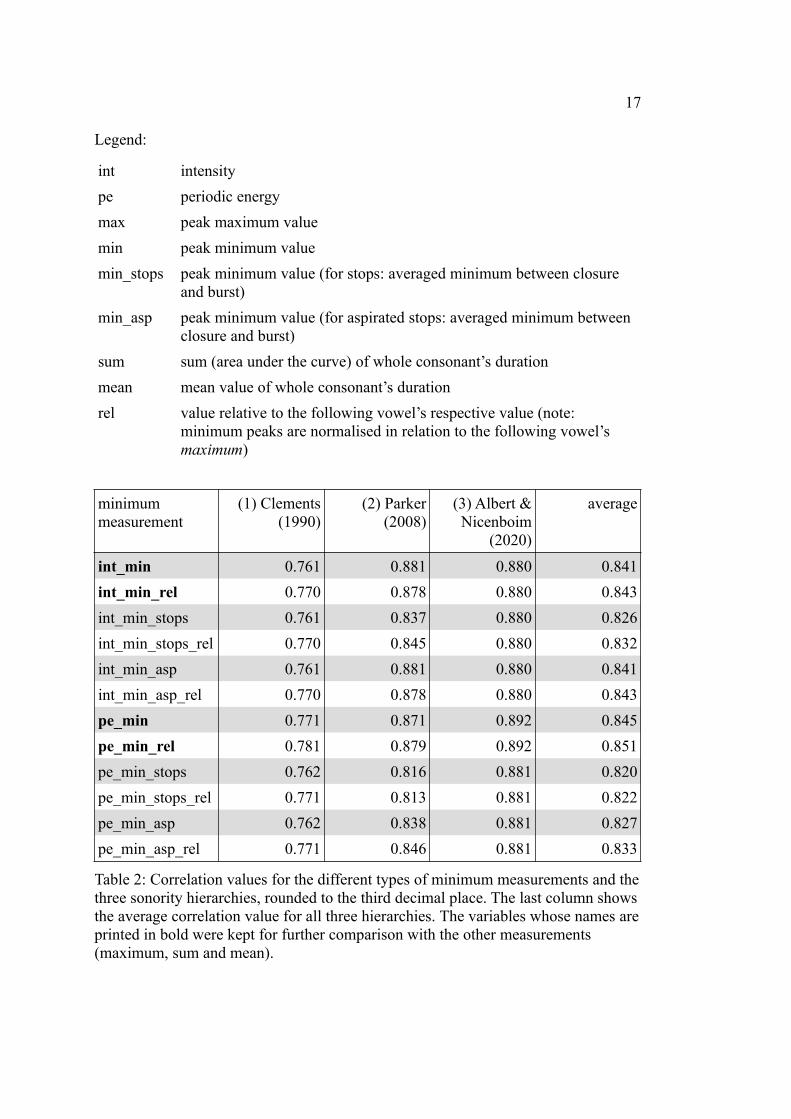
3.2 Results
In this section, I will report on the correlation results. First, I will examine the
three types of minimum measurements (see Table 2) and discard two of them from
further analysis, reducing the number of scales. Then, I will compare the remaining
results with each other (see Table 3). The legend printed below explains the variable
names for both tables.
17
Legend:
int intensity
pe periodic energy
max peak maximum value
min peak minimum value
min_stops peak minimum value (for stops: averaged minimum between closure and burst)
min_asp peak minimum value (for aspirated stops: averaged minimum between closure and burst)
sum sum (area under the curve) of whole consonant’s duration
mean mean value of whole consonant’s duration
rel value relative to the following vowel’s respective value (note: minimum peaks are normalised in relation to the following vowel’s maximum)
minimum measurement
(1) Clements(1990)
(2) Parker(2008)
(3) Albert &Nicenboim
(2020)
average
int_min 0.761 0.881 0.880 0.841
int_min_rel 0.770 0.878 0.880 0.843
int_min_stops 0.761 0.837 0.880 0.826
int_min_stops_rel 0.770 0.845 0.880 0.832
int_min_asp 0.761 0.881 0.880 0.841
int_min_asp_rel 0.770 0.878 0.880 0.843
pe_min 0.771 0.871 0.892 0.845
pe_min_rel 0.781 0.879 0.892 0.851
pe_min_stops 0.762 0.816 0.881 0.820
pe_min_stops_rel 0.771 0.813 0.881 0.822
pe_min_asp 0.762 0.838 0.881 0.827
pe_min_asp_rel 0.771 0.846 0.881 0.833
Table 2: Correlation values for the different types of minimum measurements and thethree sonority hierarchies, rounded to the third decimal place. The last column showsthe average correlation value for all three hierarchies. The variables whose names areprinted in bold were kept for further comparison with the other measurements (maximum, sum and mean).
18
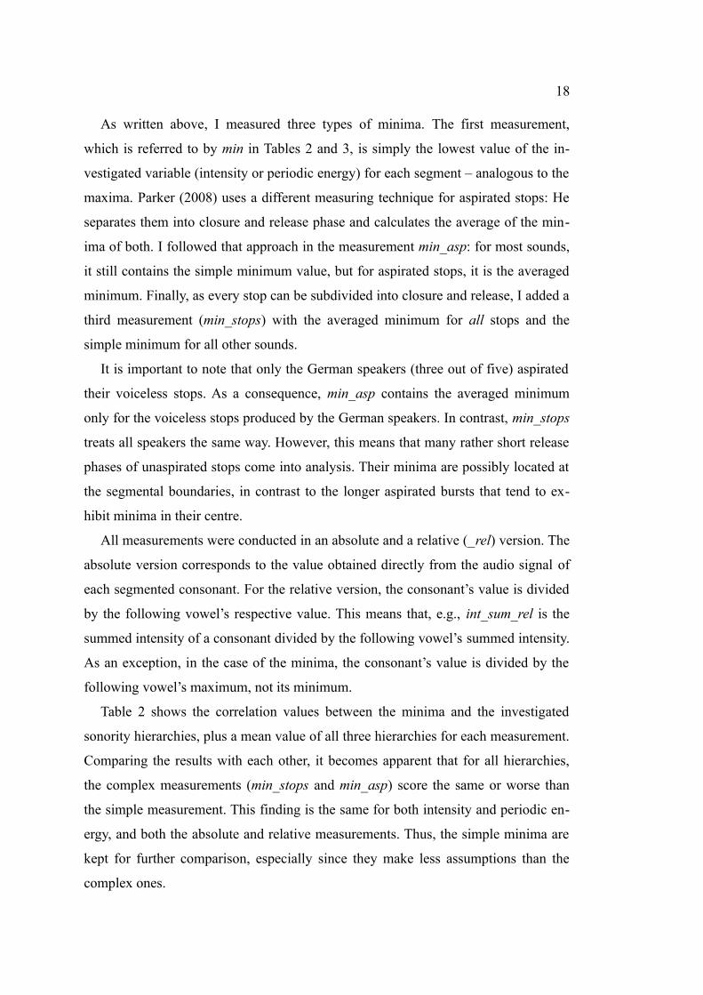
As written above, I measured three types of minima. The first measurement,
which is referred to by min in Tables 2 and 3, is simply the lowest value of the in-
vestigated variable (intensity or periodic energy) for each segment – analogous to the
maxima. Parker (2008) uses a different measuring technique for aspirated stops: He
separates them into closure and release phase and calculates the average of the min-
ima of both. I followed that approach in the measurement min_asp: for most sounds,
it still contains the simple minimum value, but for aspirated stops, it is the averaged
minimum. Finally, as every stop can be subdivided into closure and release, I added a
third measurement (min_stops) with the averaged minimum for all stops and the
simple minimum for all other sounds.
It is important to note that only the German speakers (three out of five) aspirated
their voiceless stops. As a consequence, min_asp contains the averaged minimum
only for the voiceless stops produced by the German speakers. In contrast, min_stops
treats all speakers the same way. However, this means that many rather short release
phases of unaspirated stops come into analysis. Their minima are possibly located at
the segmental boundaries, in contrast to the longer aspirated bursts that tend to ex-
hibit minima in their centre.
All measurements were conducted in an absolute and a relative (_rel) version. The
absolute version corresponds to the value obtained directly from the audio signal of
each segmented consonant. For the relative version, the consonant’s value is divided
by the following vowel’s respective value. This means that, e.g., int_sum_rel is the
summed intensity of a consonant divided by the following vowel’s summed intensity.
As an exception, in the case of the minima, the consonant’s value is divided by the
following vowel’s maximum, not its minimum.
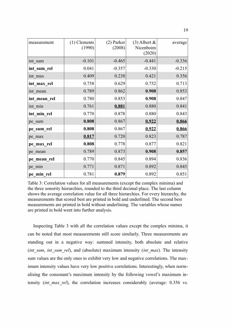
Table 2 shows the correlation values between the minima and the investigated
sonority hierarchies, plus a mean value of all three hierarchies for each measurement.
Comparing the results with each other, it becomes apparent that for all hierarchies,
the complex measurements (min_stops and min_asp) score the same or worse than
the simple measurement. This finding is the same for both intensity and periodic en-
ergy, and both the absolute and relative measurements. Thus, the simple minima are
kept for further comparison, especially since they make less assumptions than the
complex ones.
19
measurement (1) Clements(1990)
(2) Parker(2008)
(3) Albert &Nicenboim
(2020)
average
int_sum -0.101 -0.465 -0.441 -0.336
int_sum_rel 0.041 -0.357 -0.330 -0.215
int_max 0.409 0.238 0.421 0.356
int_max_rel 0.758 0.629 0.752 0.713
int_mean 0.789 0.862 0.908 0.853
int_mean_rel 0.780 0.853 0.908 0.847
int_min 0.761 0.881 0.880 0.841
int_min_rel 0.770 0.878 0.880 0.843
pe_sum 0.808 0.867 0.922 0.866
pe_sum_rel 0.808 0.867 0.922 0.866
pe_max 0.817 0.720 0.823 0.787
pe_max_rel 0.808 0.778 0.877 0.821
pe_mean 0.789 0.873 0.908 0.857
pe_mean_rel 0.770 0.845 0.894 0.836
pe_min 0.771 0.871 0.892 0.845
pe_min_rel 0.781 0.879 0.892 0.851
Table 3: Correlation values for all measurements (except the complex minima) and the three sonority hierarchies, rounded to the third decimal place. The last column shows the average correlation value for all three hierarchies. For every hierarchy, the measurements that scored best are printed in bold and underlined. The second best measurements are printed in bold without underlining. The variables whose names are printed in bold went into further analysis.
Inspecting Table 3 with all the correlation values except the complex minima, it
can be noted that most measurements still score similarly. Three measurements are
standing out in a negative way: summed intensity, both absolute and relative
(int_sum, int_sum_rel), and (absolute) maximum intensity (int_max). The intensity
sum values are the only ones to exhibit very low and negative correlations. The max-
imum intensity values have very low positive correlations. Interestingly, when norm-
alising the consonant’s maximum intensity by the following vowel’s maximum in-
tensity (int_max_rel), the correlation increases considerably (average: 0.356 vs.
20
0.713). This is the only case where the difference between a measure’s absolute and
relative version is that high.
Still, even int_max_rel exhibits, on average, considerably lower correlation values
(0.71) than the remaining 20 measures, which range between an overall average of
0.79 and 0.87. For hierarchy (1), the correlation values of those 20 measurements
range between 0.75 and 0.82. In the case of (2), they range from 0.72 to 0.88, and for
(3), a range spanning from 0.82 to 0.92 can be observed.
3.3 Analysis
For further investigation, I calculated Tukey groupings to get a better insight into
the single scales. Tukey groups indicate for each measurement which consonants dif-
fer significantly from each other. These groups can then be compared with the pro-
posed sonority hierarchies. Because a detailed comparison of all 16 scales would go
beyond the scope of this thesis, I chose to examine only one version (absolute or rel-
ative) of each measurement, ending up with eight variables.
In the case of int_max, the relative version scores much better than the absolute
one (on average, 0.713 vs. 0.356). For the other measures, the correlation values of
their absolute and relative version differ only slightly. Thus, in order to provide for
the best possible comparability, I examined the relative version of each measurement.
21
3.3.1 Peaks
3.3.1.1 Minima
consonant Minimum intensity
Tukey groups (intensity)
Minimum periodic energy
Tukey groups (periodic energy)
j 0.947 dfg 0.701 b
w 0.939 dfg 0.664 b
l 0.954 fg 0.737 b
m 0.952 efg 0.731 b
n 0.963 g 0.791 b
v 0.832 cd 0.142 a
z 0.844 cf 0.236 a
b 0.840 cf 0.105 a
d 0.837 cde 0.204 a
f 0.748 bc 0.000 a
s 0.816 c 0.000 a
p 0.605 a 0.000 a
t 0.633 ab 0.000 a
Table 4: Relative minimum values of intensity and periodic energy for each consonant with their Tukey groups. The displayed values are averaged across all speakers.
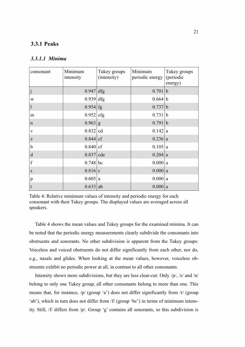
Table 4 shows the mean values and Tukey groups for the examined minima. It can
be noted that the periodic energy measurements clearly subdivide the consonants into
obstruents and sonorants. No other subdivision is apparent from the Tukey groups:
Voiceless and voiced obstruents do not differ significantly from each other, nor do,
e.g., nasals and glides. When looking at the mean values, however, voiceless ob-
struents exhibit no periodic power at all, in contrast to all other consonants.
Intensity shows more subdivisions, but they are less clear-cut: Only /p/, /s/ and /n/
belong to only one Tukey group, all other consonants belong to more than one. This
means that, for instance, /p/ (group ‘a’) does not differ significantly from /t/ (group
‘ab’), which in turn does not differ from /f/ (group ‘bc’) in terms of minimum intens-
ity. Still, /f/ differs from /p/. Group ‘g’ contains all sonorants, so this subdivision is
22
also visible for intensity. Then again, all sonorants except /n/ belong to group ‘f’,
which also the obstruents /z/ and /b/ belong to. Group ‘d’ contains the glides /j/
and /w/, but also the obstruents /v/ and /d/. So although minimum intensity exhibits
more groupings, it does not provide more clear distinctions than periodic energy.
Moreover, we can observe an interesting discrepancy between the correlation of
the minima’s mean values and the respective sonority indices on the one hand, and
their Tukey groupings on the other: Both intensity and periodic energy have similar
correlation values (averaged correlation: 0.843 (intensity) vs. 0.851 (periodic en-
ergy), cf. Table 3), but periodic energy is much better at creating groups that match
the subdivisions of the sonority hierarchies analysed in this study.
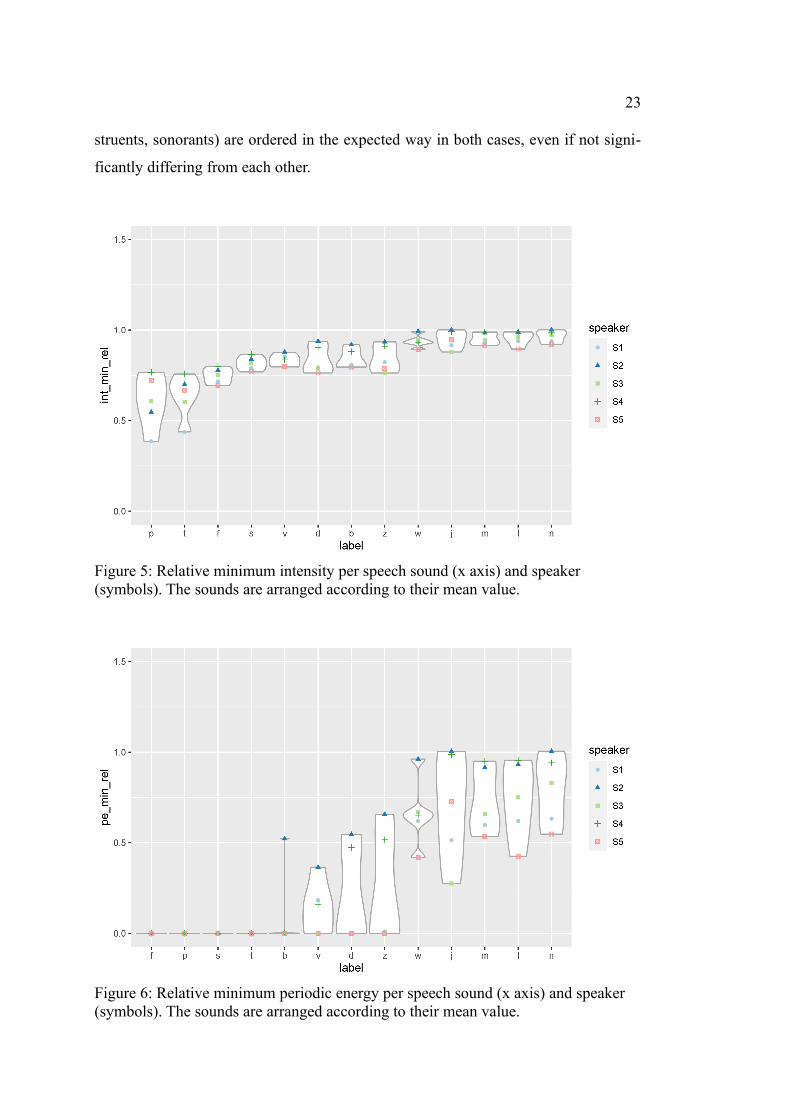
Looking at Figure 5, it becomes visible that, although minimum intensity approx-
imately shows the expected trend, the consonants are quite close to each other and do
not cover a wide range. This illustrates the unclear Tukey groups, although some of
the groups can be perceived visually: First, group ‘a’ contains the voiceless stops,
which extend over a similar range in the plot. Other than that, however, no clear dis-
tinction between voiceless and voiced obstruents is visible, especially since /s/ tends
to pattern more with the voiced ones. Second, the sonorants can be visually grouped
together, reflecting Tukey group ‘g’.
Minimum periodic energy (see Figure 6), on the other hand, provides for a much
better separation between obstruents and sonorants. Moreover, although the Tukey
groups do not subdivide obstruents into voiceless and voiced ones, this separation is
supported by the mean values (cf. Table 4) and the plot: The voiceless obstruents
consistently reach zero and show no visible variation. This result is expectable be-
cause voiceless sounds as such do not have any periodic components. As illustrated
above, the only periodic energy measured for voiceless sounds has to be attributed to
the surrounding sounds and does not have much effect on the minimum peak. The
voiced obstruents, as Figure 6 shows, show more variation: Some speakers produce
them with much more minimum periodic energy than voiceless obstruents. However,
other speakers exhibit a minimum near zero, which, apparently, makes for a too high
intersection between voiceless and voiced obstruents.
The plots illustrate that both measurements produce no perfect correlation with
any of the three hierarchies, but the major classes (voiceless obstruents, voiced ob-
23
struents, sonorants) are ordered in the expected way in both cases, even if not signi-
ficantly differing from each other.
Figure 5: Relative minimum intensity per speech sound (x axis) and speaker (symbols). The sounds are arranged according to their mean value.
Figure 6: Relative minimum periodic energy per speech sound (x axis) and speaker (symbols). The sounds are arranged according to their mean value.
24
3.3.1.2 Maxima
consonant Maximum intensity
Tukey groups (intensity)
Maximum periodic energy
Tukey groups (periodic energy)
j 1.002 f 1.017 f
w 0.983 cf 0.891 cdf
l 0.985 def 0.894 cdf
m 0.994 ef 0.946 ef
n 0.991 ef 0.944 df
v 0.958 ac 0.720 ac
z 0.942 a 0.667 ab
b 0.980 cf 0.731 ad
d 0.984 cf 0.796 bcde
f 0.944 a 0.569 a
s 0.951 ab 0.559 a
p 0.971 bce 0.730 ad
t 0.962 acd 0.644 ab
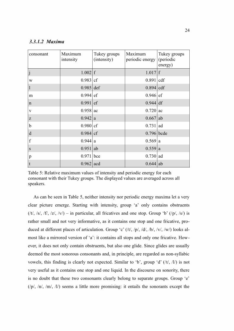
Table 5: Relative maximum values of intensity and periodic energy for each consonant with their Tukey groups. The displayed values are averaged across all speakers.
As can be seen in Table 5, neither intensity nor periodic energy maxima let a very
clear picture emerge. Starting with intensity, group ‘a’ only contains obstruents
(/t/, /s/, /f/, /z/, /v/) – in particular, all fricatives and one stop. Group ‘b’ (/p/, /s/) is
rather small and not very informative, as it contains one stop and one fricative, pro-
duced at different places of articulation. Group ‘c’ (/t/, /p/, /d/, /b/, /v/, /w/) looks al-
most like a mirrored version of ‘a’: it contains all stops and only one fricative. How-
ever, it does not only contain obstruents, but also one glide. Since glides are usually
deemed the most sonorous consonants and, in principle, are regarded as non-syllabic
vowels, this finding is clearly not expected. Similar to ‘b’, group ‘d’ (/t/, /l/) is not
very useful as it contains one stop and one liquid. In the discourse on sonority, there
is no doubt that these two consonants clearly belong to separate groups. Group ‘e’
(/p/, /n/, /m/, /l/) seems a little more promising: it entails the sonorants except the
25
glides, but, oddly, a stop as well. The final group, ‘f’ (/d/, /b/, /n/, /m/, /l/, /w/, /j/),
contains all sonorants and the voiced stops.
As for periodic energy, group ‘f’ encompasses all sonorants. However, this is the
only clear match between the maxima Tukey groups and the classes in the sonority
hierarchies. Group ‘a’ is almost a perfect counterpart, containing all obstruents ex-
cept /d/. All other groups are, similar to those of the intensity maxima, not very in-
formative, since no tendency of a match between them and sonority groupings can be
observed.
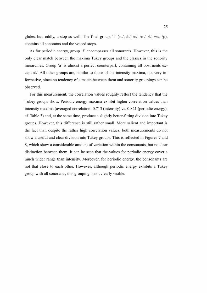
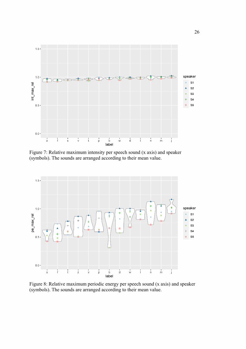
For this measurement, the correlation values roughly reflect the tendency that the
Tukey groups show. Periodic energy maxima exhibit higher correlation values than
intensity maxima (averaged correlation: 0.713 (intensity) vs. 0.821 (periodic energy),
cf. Table 3) and, at the same time, produce a slightly better-fitting division into Tukey
groups. However, this difference is still rather small. More salient and important is
the fact that, despite the rather high correlation values, both measurements do not
show a useful and clear division into Tukey groups. This is reflected in Figures 7 and
8, which show a considerable amount of variation within the consonants, but no clear
distinction between them. It can be seen that the values for periodic energy cover a
much wider range than intensity. Moreover, for periodic energy, the consonants are
not that close to each other. However, although periodic energy exhibits a Tukey
group with all sonorants, this grouping is not clearly visible.
26
Figure 7: Relative maximum intensity per speech sound (x axis) and speaker (symbols). The sounds are arranged according to their mean value.
Figure 8: Relative maximum periodic energy per speech sound (x axis) and speaker (symbols). The sounds are arranged according to their mean value.
27
3.3.2 Sum
consonant Summed intensity
Tukey groups (intensity)
Summed periodic energy
Tukey groups (periodic energy)
j 0.695 bc 0.670 c
w 0.537 ab 0.493 bc
l 0.580 ac 0.518 c
m 0.638 ac 0.626 c
n 0.585 ac 0.588 c
v 0.526 ab 0.238 ab
z 0.415 a 0.166 a
b 0.545 ac 0.217 a
d 0.527 ab 0.219 a
f 0.658 ac 0.072 a
s 0.788 c 0.072 a
p 0.695 bc 0.145 a
t 0.734 bc 0.110 a
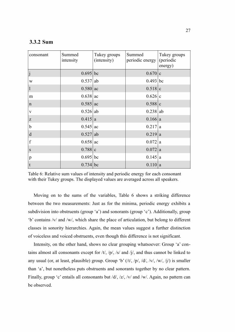
Table 6: Relative sum values of intensity and periodic energy for each consonant with their Tukey groups. The displayed values are averaged across all speakers.
Moving on to the sums of the variables, Table 6 shows a striking difference
between the two measurements: Just as for the minima, periodic energy exhibits a
subdivision into obstruents (group ‘a’) and sonorants (group ‘c’). Additionally, group
‘b’ contains /v/ and /w/, which share the place of articulation, but belong to different
classes in sonority hierarchies. Again, the mean values suggest a further distinction
of voiceless and voiced obstruents, even though this difference is not significant.
Intensity, on the other hand, shows no clear grouping whatsoever: Group ‘a’ con-
tains almost all consonants except for /t/, /p/, /s/ and /j/, and thus cannot be linked to
any usual (or, at least, plausible) group. Group ‘b’ (/t/, /p/, /d/, /v/, /w/, /j/) is smaller
than ‘a’, but nonetheless puts obstruents and sonorants together by no clear pattern.
Finally, group ‘c’ entails all consonants but /d/, /z/, /v/ and /w/. Again, no pattern can
be observed.
28
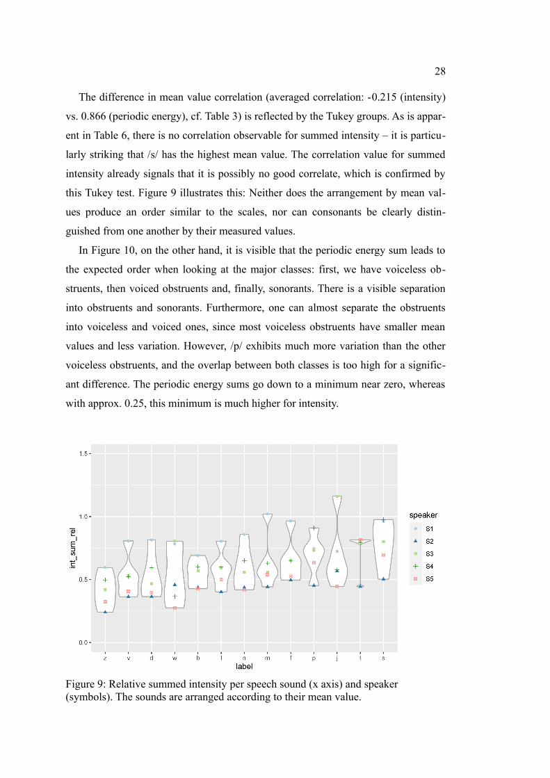
The difference in mean value correlation (averaged correlation: -0.215 (intensity)
vs. 0.866 (periodic energy), cf. Table 3) is reflected by the Tukey groups. As is appar-
ent in Table 6, there is no correlation observable for summed intensity – it is particu-
larly striking that /s/ has the highest mean value. The correlation value for summed
intensity already signals that it is possibly no good correlate, which is confirmed by
this Tukey test. Figure 9 illustrates this: Neither does the arrangement by mean val-
ues produce an order similar to the scales, nor can consonants be clearly distin-
guished from one another by their measured values.
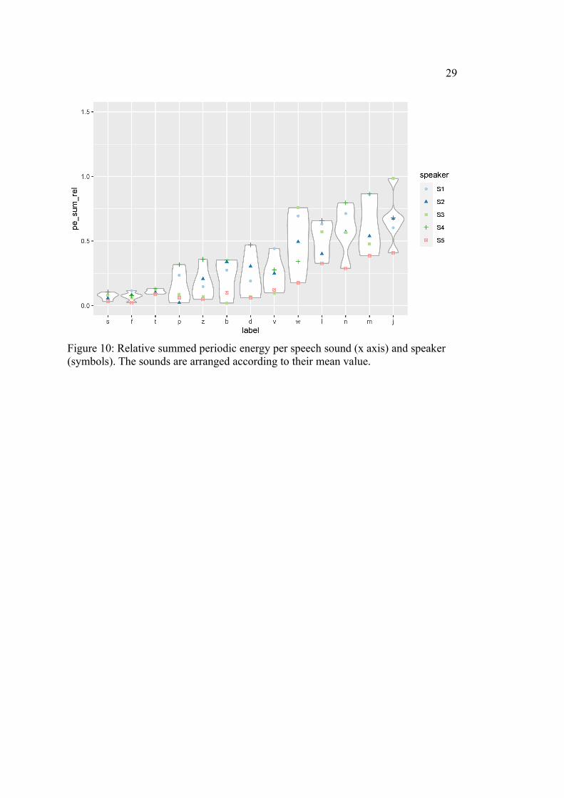
In Figure 10, on the other hand, it is visible that the periodic energy sum leads to
the expected order when looking at the major classes: first, we have voiceless ob-
struents, then voiced obstruents and, finally, sonorants. There is a visible separation
into obstruents and sonorants. Furthermore, one can almost separate the obstruents
into voiceless and voiced ones, since most voiceless obstruents have smaller mean
values and less variation. However, /p/ exhibits much more variation than the other
voiceless obstruents, and the overlap between both classes is too high for a signific-
ant difference. The periodic energy sums go down to a minimum near zero, whereas
with approx. 0.25, this minimum is much higher for intensity.
Figure 9: Relative summed intensity per speech sound (x axis) and speaker (symbols). The sounds are arranged according to their mean value.
29
Figure 10: Relative summed periodic energy per speech sound (x axis) and speaker (symbols). The sounds are arranged according to their mean value.
30
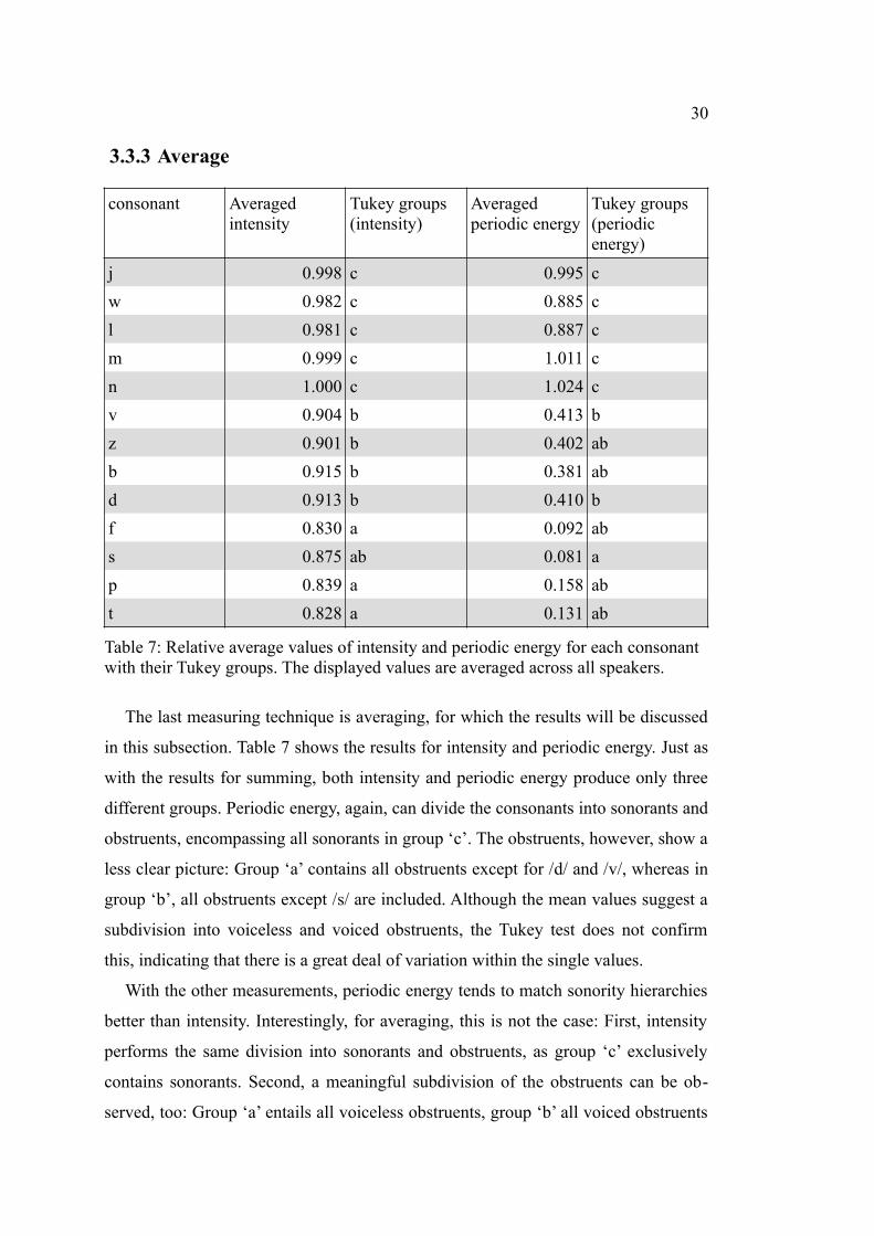
3.3.3 Average
consonant Averaged intensity
Tukey groups (intensity)
Averaged periodic energy
Tukey groups (periodic energy)
j 0.998 c 0.995 c
w 0.982 c 0.885 c
l 0.981 c 0.887 c
m 0.999 c 1.011 c
n 1.000 c 1.024 c
v 0.904 b 0.413 b
z 0.901 b 0.402 ab
b 0.915 b 0.381 ab
d 0.913 b 0.410 b
f 0.830 a 0.092 ab
s 0.875 ab 0.081 a
p 0.839 a 0.158 ab
t 0.828 a 0.131 ab
Table 7: Relative average values of intensity and periodic energy for each consonant with their Tukey groups. The displayed values are averaged across all speakers.
The last measuring technique is averaging, for which the results will be discussed
in this subsection. Table 7 shows the results for intensity and periodic energy. Just as
with the results for summing, both intensity and periodic energy produce only three
different groups. Periodic energy, again, can divide the consonants into sonorants and
obstruents, encompassing all sonorants in group ‘c’. The obstruents, however, show a
less clear picture: Group ‘a’ contains all obstruents except for /d/ and /v/, whereas in
group ‘b’, all obstruents except /s/ are included. Although the mean values suggest a
subdivision into voiceless and voiced obstruents, the Tukey test does not confirm
this, indicating that there is a great deal of variation within the single values.
With the other measurements, periodic energy tends to match sonority hierarchies
better than intensity. Interestingly, for averaging, this is not the case: First, intensity
performs the same division into sonorants and obstruents, as group ‘c’ exclusively
contains sonorants. Second, a meaningful subdivision of the obstruents can be ob-
served, too: Group ‘a’ entails all voiceless obstruents, group ‘b’ all voiced obstruents
31
and, in addition, /s/. Disregarding this potential artefact, average intensity comes
closest – out of all measurements – to hierarchy (3) by Albert and Nicenboim (2020),
which otherwise only separates glides from the other sonorants.
Since the average values are based on the same calculation as summing and, as the
only additional step, normalise this by the consonants’ duration, a comparison
between these is useful. For periodic energy, summing produces a clearer result than
averaging, although the main subdivision (sonorants vs. obstruents) becomes appar-
ent in both cases and both have a similar correlation (averaged correlation: 0.866
(sum) vs. 0.836 (average), cf. Table 3). Regarding intensity, there is a great discrep-
ancy between summing and averaging: Summing does not lead to usable results at
all, as no correlation with any of the three examined sonority hierarchies is observ-
able and no meaningful Tukey group can be established. Averaging, on the other
hand, produces very clear groups, even the clearest of all investigated measurements.
However, it can be concluded that periodic energy is more robust with regard to dur-
ation, because useful results are obtained in both cases and not only in the average.
Similar to summing, the correlation values for averaging (averaged correlation:
0.847 (intensity) vs. 0.836 (periodic energy), cf. Table 3) are a proper reflection of
the goodness of fit for the Tukey groups. However, although intensity has a slightly
better correlation and slightly better-fitting Tukey groups, it is important to note that
the values do not cover a wide range and the effects are rather small (see Figure 11)
compared to periodic energy (see Figure 12).
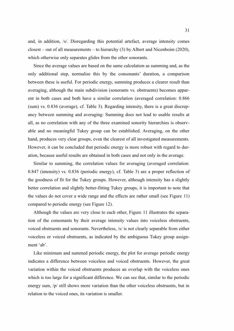
Although the values are very close to each other, Figure 11 illustrates the separa-
tion of the consonants by their average intensity values into voiceless obstruents,
voiced obstruents and sonorants. Nevertheless, /s/ is not clearly separable from either
voiceless or voiced obstruents, as indicated by the ambiguous Tukey group assign-
ment ‘ab’.
Like minimum and summed periodic energy, the plot for average periodic energy
indicates a difference between voiceless and voiced obstruents. However, the great
variation within the voiced obstruents produces an overlap with the voiceless ones
which is too large for a significant difference. We can see that, similar to the periodic
energy sum, /p/ still shows more variation than the other voiceless obstruents, but in
relation to the voiced ones, its variation is smaller.
32
Figure 11: Relative average intensity per speech sound (x axis) and speaker (symbols). The sounds are arranged according to their mean value.
Figure 12: Relative average periodic energy per speech sound (x axis) and speaker (symbols). The sounds are arranged according to their mean value.
33
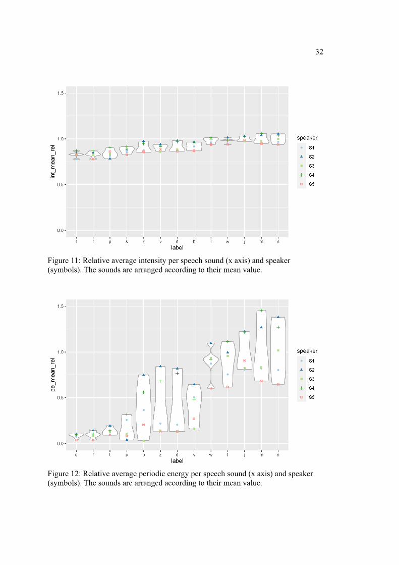
3.4 Discussion
This study provides a large amount of results which lead to interesting findings. In
the following subsections, I will discuss the results for summing (subsection 3.4.1),
peaks (subsection 3.4.2) and averaging (subsection 3.4.3). Finally, I will present
some general remarks on this study (subsection 3.4.4).
3.4.1 The role of duration: Summing makes a difference
Summing produces the highest discrepancy between intensity and periodic en-
ergy: The periodic energy sum has very good correlation values, even the best among
all measures (averaged across all hierarchies), and produces useful Tukey groups. In-
tensity, on the other hand, produces the worst values of all, with a correlation near
zero or low negative correlations. Aside from that, no useful Tukey groups can be es-
tablished. Thus, summed intensity does not produce any sonority-relevant grouping
pattern, whereas summed periodic energy turns out to exhibit a general pattern of
sonority-relevant grouping.
Why is this the case? First, one has to keep in mind how the investigated variables
relate to each other: Intensity refers to the power of the acoustic signal. Periodic en-
ergy can be seen as a subpart of general intensity, as it refers to the intensity of the
signal’s periodic components. Since only voiced consonants exhibit periodic com-
ponents, voiceless consonants are bound to have a low periodic energy sum – their
only periodic components have to be attributed to surrounding voiced segments. This
is in line with the fact that voiceless sounds are considered least sonorous in all ex-
amined sonority hierarchies. In contrast, intensity is not necessarily low for voiceless
sounds, as it measures the whole power of the signal, including aperiodic compon-
ents such as friction. This becomes apparent in the analysis, where /s/ has, on aver-
age, the highest intensity sum, and all other voiceless sounds tend to rank high, too.
Moreover, even though voiced obstruents have periodic components, the rather high
constriction in the vocal tract dampens them. This, again, fits most sonority hierarch-
ies that are part of this study, as voiced obstruents are often considered more sonor-
ous than voiceless ones, and always considered to be less sonorous than sonorants.
For these reasons, summed periodic energy is generally expected to produce good
results. Why, on the other hand, does summed intensity produce so bad results, espe-
34
cially given the fact that intensity produces rather good results in other measure-
ments? Particularly, average intensity leads to good correlation and grouping results.
Importantly, the average measurement is related very closely to summing: A conson-
ant’s sum (of intensity or periodic energy) is divided by its duration to neutralise its
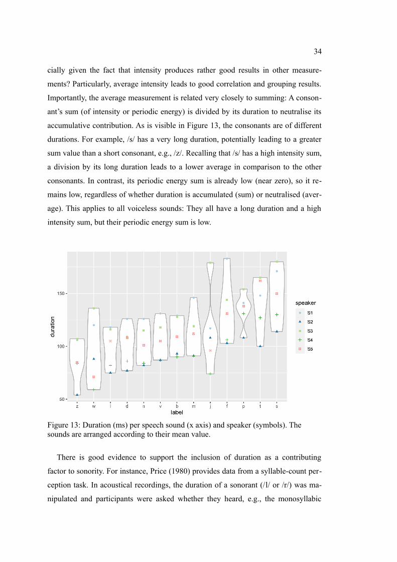
accumulative contribution. As is visible in Figure 13, the consonants are of different
durations. For example, /s/ has a very long duration, potentially leading to a greater
sum value than a short consonant, e.g., /z/. Recalling that /s/ has a high intensity sum,
a division by its long duration leads to a lower average in comparison to the other
consonants. In contrast, its periodic energy sum is already low (near zero), so it re-
mains low, regardless of whether duration is accumulated (sum) or neutralised (aver-
age). This applies to all voiceless sounds: They all have a long duration and a high
intensity sum, but their periodic energy sum is low.
Figure 13: Duration (ms) per speech sound (x axis) and speaker (symbols). The sounds are arranged according to their mean value.
There is good evidence to support the inclusion of duration as a contributing
factor to sonority. For instance, Price (1980) provides data from a syllable-count per-
ception task. In acoustical recordings, the duration of a sonorant (/l/ or /r/) was ma-
nipulated and participants were asked whether they heard, e.g., the monosyllabic

35
word ‘plight’ /plʌɪt/ or the disyllabic word ‘polite’/pəˈlʌɪt/. The longer the duration of
the sonorant, the more the word is perceived as disyllabic, and, as a consequence, the
more sonorous does the consonant appear.
This shows that duration plays a role in the sonority status of voiced consonants.
The periodic energy sum takes this into account, with longer duration leading to
higher sonority. Long voiceless sounds, on the other hand, still have a periodic en-
ergy sum near zero and presumably do not substantially increase in sonority. For ex-
ample, a lengthened /s/ in ‘scum’ /skʌm/ would probably not make people perceive
the word ‘succumb’ /səˈkʌm/: /s/ has no periodic energy and should therefore not
lead to the perception of a vowel.
3.4.2 The role of segmentation: Why min is better than max
The peak measurements all produce rather good correlation values (between 0.71
and 0.85), but only minimum periodic energy produces a clear subdivision of the
consonants, namely into obstruents and sonorants. This subdivision is somewhat no-
ticeable for minimum intensity and maximum periodic energy, too, but much less
clear-cut. Maximum intensity does not produce any useful Tukey groups at all.
The fact that minima score better than maxima can be explained as follows:
Mostly, consonants exhibit lower values of intensity and periodic energy than sur-
rounding vowels. Hence, consonantal minima of intensity and periodic energy are
likely to occur in the middle of their segment. This makes the minima very robust to
segmentation: Slight changes in position of the segmental boundaries should have no
effect on the minimum, which should still be found (approximately) in the conson-
ant’s centre. Maxima, on the other hand, often occur right at the segmental boundar-
ies – with the setup of this study, because every measured consonant is surrounded
by vowels. Thus, the maxima might not be attributed to the consonant as such, but to
the preceding or following vowel. In such a case, segmentation has a direct impact
on the consonant’s maximum value and is likely to skew the results. This is espe-
cially true for periodic energy of voiceless sounds: They do not exhibit any periodic
energy themselves, so their maximum periodic energy can only originate from the
surrounding vowels.
This issue can also explain the fact that absolute maximum intensity scores far
worse than its relative counterpart: Variation in the intensity of the following vowel
36
very likely leads to variation in the consonant’s maximum. When normalising in rela-
tion to the following vowel’s maximum intensity, this variation is decreased and the
results appear less skewed.
The Tukey analysis of the peak measurements shows that it is not sufficient to
only compare correlation values. Furthermore, this study shows that a minimum
measurement that averages closure and burst of aspirated consonants, as Parker
(2008) proposed, does not have any benefit on the correlation values. In summary,
minimum values can, especially with periodic energy, form a rather good correlate
for sonority. It should be noted, however, that peak values (minimum and maximum)
only consider one point in time. In the case of laboratory experiments, minima ap-
pear to be a rather robust cue. Though, they might be sensitive to, e.g., background
noise in everyday recordings, or signal distortions. Summing and averaging, in con-
trast, take the whole consonant’s duration into account and are thus more robust
against that.
3.4.3 The mean between: The robustness of the average measure
In contrast to summing and peak measurements, the average measure turns out to
produce good results in every case: both intensity and periodic energy, both the abso-
lute and relative version. The reasons as to why the intensity average performs much
better than summed intensity have been discussed above and are summarised again
here: Especially voiceless sounds, i.e. sounds with the lowest sonority values, tend to
have a long duration that can play a role when summing is applied on a general
acoustic dimension such as intensity. Averaging, in contrast to summing, neutralises
the duration component, which results in lower intensity measurements for these
sounds. Their periodic energy, on the other hand, is already near zero, so periodic en-
ergy measures remain low for voiceless obstruents even when the values accumulate
for the duration of the consonant. Moreover, the average intensity values cover a
smaller range than average periodic energy. This reflects the fact that the intensity
sum values are very close to each other and the normalisation by duration does pro-
duce significant differences, but still, rather small ones.
As stated above, there is evidence that duration is relevant with respect to sonority
– especially for voiced sounds. Following this assumption, the periodic energy sum
appears as the most suitable measurement: The sum increases with a longer duration,
37
and periodic energy leads to the desirable difference in the accumulative effect of
summing, which is strong for sonorants and weak for obstruents, especially voice-
less. An average, in contrast, does not change substantially with a change in duration.
Thus, this type of measurement would not account for the fact that, e.g., a long son-
orant could be perceived as more sonorous. Nevertheless, it still provides a good ap-
proximation, as demonstrated in this study. Especially in cases where, for instance,
only intensity values can be examined, or the contribution of duration is not certain,
measuring the average is a good approach for a sonority correlate. In addition, it is
not as sensitive to minor signal distortions as peaks can be. Although averaging
might not be the best approach in every case, the results of this study suggest that it
is a very robust one.
3.4.4 General remarks
Across the board, no measurement subdivides the investigated consonants as fine-
grained as any of the considered sonority hierarchies. The most frequent subdivision
is into obstruents and sonorants. One measurement additionally produces a signific-
ant distinction of voiceless and voiced obstruents (with one ambiguously assigned
consonant), and some more measures show a tendency towards this when averaging
across all speakers. A follow-up study with more participants might produce a clearer
picture. Moreover, it is still important to note that most measurements result in rather
high correlation values and thus encompass at least some aspect of sonority.
Regarding the sonorants, this study does not provide evidence for a further subdi-
vision based on the conducted measurements. Especially, /w/ often exhibits the low-
est values of all sonorants, but being a glide, it has the highest sonority values in all
of the three investigated sonority hierarchies. It has to be noted, though, that the val-
ues show a considerable amount of variation. Again, a study with more participants
and more stimuli could produce a different picture.
Generally speaking, this study is of limited statistical power, due to the low num-
ber of participants. A larger amount of stimuli – and perhaps more natural and di-
verse ones – would also be beneficial for a following study’s explanatory power.
However, when changing the stimuli from pseudowords to natural words, possible
effects of lexical frequency should be considered.
38
4 Conclusion
This exploratory study contributes to the ongoing debate on the nature of sonority
and the question whether it can be measured physically. To approach this problem, I
conducted several acoustic measurements on recorded consonants and calculated cor-
relations with three different prototypical sonority hierarchies. Following, I analysed
the different types of measurements more closely in order to find possible groups
among the consonants.
The results show that most measurements lead to rather high correlation values.
Moreover, the consonants often subdivide into obstruents and sonorants, and a tend-
ency to divide obstruents into voiceless and voiced ones is visible. This shows that
sonority can, at least in part, be measured physically.
None of the measurements produces a perfect correlation with any of the con-
sidered sonority hierarchies. However, a perfect correlation might not even be real-
istic, since speech sounds are not bound to have fixed sonority values. For instance,
there is evidence for effects of segmental duration on sonority: Voiced consonants
tend to be perceived as more sonorous when lengthened. This contradicts the idea of
fixed sonority values, which all symbolic sonority hierarchies are based on.
Nevertheless, the measurement of summed periodic energy actually takes the ef-
fect of duration into account: Voiced sounds, especially sonorants, have a substan-
tially higher periodic energy sum with a longer duration. Thus, this measurement
supports the idea that speech sounds do not have fixed sonority values and, probably,
no perfect correlate is expectable. This reflects the general problem of examining
continuous natural language by means of discrete symbols.
On the one hand, summed periodic energy supports the idea that a perfect correla-
tion could be impossible. On the other hand, of all measurements in this study, it still
comes closest to being perfect. This additionally corroborates the assumption that
periodic energy is essential to sonority.
Looking at the average measurement, both examined variables perform well. If
periodic energy cannot be obtained, average intensity seems to be a good approxima-
tion to sonority – in contrast to summed intensity, which is not useful at all. Of the
peak values, especially minimum periodic energy shows good results. Minimum in-
39
tensity shows a good correlation as well, but less clear groups of consonants. Finally,
at least for consonants, maximum peaks are no reliable cue to sonority.
As already stated, this is an exploratory pilot study with few participants and
therefore limited statistical power. Still, it provides interesting findings that can be
the basis of further examination. Future studies with more participants could analyse
more speech sounds in varying prosodic conditions. Moreover, a broad bandwidth of
languages would be beneficial for a cross-linguistic judgment on sonority.
This study did not find significant differences within the group of sonorants, al-
though many proposed sonority hierarchies further subdivide this group. It should be
interesting to see whether follow-up studies confirm any subdivision. The results can
then be taken as an indication of how fine-grained a sonority hierarchy should be de-
signed. This study suggests a rather coarse setup of such hierarchies, particularly
considering the idea that speech sounds are not likely to have fixed sonority values.
40
References
Albert, Aviad, Francesco Cangemi & Martine Grice (2018). Using periodic energy to
enrich acoustic representations of pitch in speech: A demonstration. Proceedings
of Speech Prosody (9), Poznań, 804–808.
Albert, Aviad & Bruno Nicenboim (2020). Take a NAP: A new model of sonority
using periodic energy and the Nucleus Attraction Principle. Manuscript submitted
for publication.
Albert, Aviad, Francesco Cangemi & Martine Grice (2020). Periogram Projekt:
Workflows for periodic energy extraction and usage. OSF. Obtained on 2020-03-
11. doi:10.17605/OSF.IO/28EA5.
Bell-Berti, Fredericka & Katherine S. Harris (1981). A temporal model of speech
production. Phonetica 38(1–3): 9–20.
Boersma, Paul & David Weenink (2020). Praat: Doing phonetics by computer.
Version 6.1.13. Retrieved from http://www.praat.org/
Browman, Catherine P. & Louis Goldstein (1992). Articulatory phonology: An
overview. Phonetica 49(3–4), 155–180.
Clements, George Nickerson (1990). The role of the sonority cycle in core
syllabification. In Kingston, John & Mary E. Beckman (eds.), Papers in
laboratory phonology 1: Between the grammar and physics of speech. Cambridge:
Cambridge University Press, 283–333.
Gordon, Matthew (2004). Syllable weight. In Hayes, Bruce (ed.), Phonetically based
phonology. Cambridge: Cambridge University Press, 277–312.
Gordon, Matthew, Edita Ghushchyan, Bradley McDonnell, Daisy Rosenblum &
Patricia A. Shaw (2012). Sonority and central vowels: A cross‐linguistic phonetic
study. In Parker, Steve (ed.), The Sonority Controversy. Berlin: De Gruyter
Mouton, 219–256.
Heselwood, Barry (1998). An unusual kind of sonority and its implications for
phonetic theory. Leeds Working Papers in Linguistics & Phonetics 6, 68–80.
ITU-R Recommendation BS.1770-4 (2015). Algorithms to measure audio
programme loudness and true-peak audio level. Geneva: ITU. BS Series:
Broadcasting service (sound).
41
Jany, Carmen, Matthew Gordon, Carlos M. Nash & Nobutaka Takara (2007). How
universal is the sonority hierarchy?: A cross-linguistic acoustic study. Proceedings
of the 16th ICPhS, Saarbrücken, 1401–1404.
Kawai, Goh & Jan van Santen (2002). Automatic detection of syllabic nuclei using
acoustic measures. Proceedings of 2002 IEEE Workshop on Speech Synthesis,
Santa Monica, 39–42.
Kawasaki, Haruko (1982). An acoustical basis for universal constraints on sound
sequences. PhD thesis. UC Berkeley: Department of Linguistics.
Komatsu, Masahiko, Shinichi Tokuma, Won Tokuma & Takayuki Arai (2002).
Multi‐dimensional analysis of sonority: Perception, acoustics, and phonology. In-
terspeech 2002: 7th International Conference on Spoken Language Processing,
Denver, Colorado, 2293–2296.
Ladefoged, Peter (1997). Linguistic phonetic descriptions. In Hardcastle, William J.
& John Laver (eds.), The handbook of phonetic sciences. Oxford; Cambridge,
MA: Blackwell, 589–618.
Llanos, Fernando, Joshua M. Alexander & Christian E. Stilp (2015). Shannon en-
tropy predicts the sonority status of natural classes in English. Poster presented at
the 169th Meeting of the Acoustical Society of America, Pittsburgh, Pennsylvania.
Nakajima, Yoshitaka, Kazuo Ueda, Shota Fujmaru, Hirotoshi Motomura & Yuki Oh-
saka (2012). Acoustic correlate of phonological sonority in British English. Pro-
ceedings of Fechner Day 28, 56–61.
Ohala, John J. (1992). Alternatives to the sonority hierarchy for explaining segmental
sequential constraints. Papers from the parasession on the syllable, Chicago, 319–
338.
Parker, Steve (2002). Quantifying the sonority hierarchy. PhD thesis. Amherst:
University of Massachusetts.
Parker, Steve (2008). Sound level protrusions as physical correlates of sonority.
Journal of phonetics 36(1), 55–90.
Parker, Steve (2011). Sonority. In van Oostendorp, Marc, Colin J. Ewen, Elizabeth
Hume & Keren Rice (eds.) The Blackwell companion to phonology 2. West
Sussex, UK: Wiley-Blackwell, 1160–1184.
42
Parker, S. (2017). Sounding out sonority. Language & Linguistics Compass 11(9), 1–
197.
Patha, Sreedhar, Yegnanarayana Bayya, and Suryakanth V. Gangashetty (2016).
Syllable nucleus and boundary detection in noisy conditions. Proceedings of
Speech Prosody (8), Boston, 360–364.
Price, Patti J. (1980). Sonority and syllabicity: Acoustic correlates of perception.
Phonetica 37(5–6), 327–343.
R Core Team (2020). R: A language and environment for statistical computing. R
Foundation for Statistical Computing, Vienna, Austria. Retrieved from
https://www.R-project.org/
Selkirk, Elisabeth (1984). On the major class features and syllable theory. In Aronoff,
Mark, Richard T. Oehrle & Morris Halle (eds.), Language sound and structure:
Studies in phonology presented to Morris Halle by his teacher and students (pp.).
Cambridge, MA: The MIT Press, 107–136.
Sievers, Eduard (1893/1901). Grundzüge der Phonetik zur Einführung in das
Studium der Lautlehre der indogermanischen Sprachen. Leipzig: Breitkopf &
Härtel.
Steriade, Donca (1982). Greek prosodies and the nature of syllabification. PhD
thesis. Massachusetts: MIT.
Eidesstattliche Versicherung
Hiermit versichere ich an Eides statt, dass ich diese Bachelorarbeit selbstständig
verfasst und ohne die Benutzung anderer als der angegebenen Hilfsmittel angefertigt
habe.
Die Stellen meiner Arbeit, die wörtlich oder sinngemäß aus veröffentlichten und
nicht veröffentlichten Schriften entnommen wurden, sind als solche unter Angabe der
Quelle kenntlich gemacht.
_____________________
Tobias Schröer