Embed Size (px)
Citation preview

Atmos. Meas. Tech., 4, 2685–2715, 2011www.atmos-meas-tech.net/4/2685/2011/doi:10.5194/amt-4-2685-2011© Author(s) 2011. CC Attribution 3.0 License.
AtmosphericMeasurement
Techniques
Inversion of tropospheric profiles of aerosol extinction and HCHOand NO2 mixing ratios from MAX-DOAS observations in Milanoduring the summer of 2003 and comparison with independentdata sets
T. Wagner1, S. Beirle1, T. Brauers2, T. Deutschmann3, U. Frieß3, C. Hak3,*, J. D. Halla4, K. P. Heue1,W. Junkermann5, X. Li 2, U. Platt3, and I. Pundt-Gruber3,**
1Max-Planck-Institut fur Chemie, Mainz, Germany2Institute fur Energie- und Klimaforschung Troposphare (IEK-8), Forschungszentrum Julich, Germany3Institute for Environmental Physics, University of Heidelberg, Germany4Centre for Atmospheric Chemistry, York University, Toronto, ON, Canada5Institute for Meteorology and Climate Research, IMK-IFU, Karlsruhe Institute of Technology,Garmisch-Partenkirchen, Germany* now at: Norwegian Institute for Air Research, Kjeller, Norway** now at: Johannes-Kepler-Gymnasium, Weil der Stadt, Germany
Received: 22 April 2011 – Published in Atmos. Meas. Tech. Discuss.: 22 June 2011Revised: 4 November 2011 – Accepted: 24 November 2011 – Published: 12 December 2011
Abstract. We present aerosol and trace gas profiles derivedfrom MAX-DOAS observations. Our inversion scheme isbased on simple profile parameterisations used as input foran atmospheric radiative transfer model (forward model).From a least squares fit of the forward model to the MAX-DOAS measurements, two profile parameters are retrievedincluding integrated quantities (aerosol optical depth or tracegas vertical column density), and parameters describing theheight and shape of the respective profiles. From these re-sults, the aerosol extinction and trace gas mixing ratios canalso be calculated. We apply the profile inversion to MAX-DOAS observations during a measurement campaign in Mi-lano, Italy, September 2003, which allowed simultaneousobservations from three telescopes (directed to north, west,south). Profile inversions for aerosols and trace gases werepossible on 23 days. Especially in the middle of the cam-paign (17–20 September 2003), enhanced values of aerosoloptical depth and NO2 and HCHO mixing ratios were found.The retrieved layer heights were typically similar for HCHOand aerosols. For NO2, lower layer heights were found,which increased during the day.
Correspondence to:T. Wagner([email protected])
The MAX-DOAS inversion results are compared to inde-pendent measurements: (1) aerosol optical depth measuredat an AERONET station at Ispra; (2) near-surface NO2 andHCHO (formaldehyde) mixing ratios measured by long pathDOAS and Hantzsch instruments at Bresso; (3) vertical pro-files of HCHO and aerosols measured by an ultra light air-craft. Depending on the viewing direction, the aerosol op-tical depths from MAX-DOAS are either smaller or largerthan those from AERONET observations. Similar compari-son results are found for the MAX-DOAS NO2 mixing ra-tios versus long path DOAS measurements. In contrast,the MAX-DOAS HCHO mixing ratios are generally higherthan those from long path DOAS or Hantzsch instruments.The comparison of the HCHO and aerosol profiles from theaircraft showed reasonable agreement with the respectiveMAX-DOAS layer heights. From the comparison of the re-sults for the different telescopes, it was possible to investigatethe internal consistency of the MAX-DOAS observations.
As part of our study, a cloud classification algorithm wasdeveloped (based on the MAX-DOAS zenith viewing direc-tions), and the effects of clouds on the profile inversion wereinvestigated. Different effects of clouds on aerosols and tracegas retrievals were found: while the aerosol optical depth issystematically underestimated and the HCHO mixing ratiois systematically overestimated under cloudy conditions, the
Published by Copernicus Publications on behalf of the European Geosciences Union.

2686 T. Wagner et al.: Tropospheric trace gas and aerosol profiles from MAX DOAS
NO2 mixing ratios are only slightly affected. These findingsare in basic agreement with radiative transfer simulations.
1 Introduction
MAX-DOAS instruments measure scattered sun light fromdifferent, mostly slant elevation angles, thus having a highsensitivity to trace gases and aerosols located close to theEarth’s surface (e.g. Honninger et al., 2002; Van Roozen-dael et al., 2003; Wittrock et al., 2004; Wagner et al., 2004;Brinksma et al., 2008 and references therein). In addition tothe retrieval of trace gas mixing ratios or aerosol extinctionclose to the surface, information on vertical profiles and ver-tically integrated quantities (vertical trace gas column density(VCD) or aerosol optical depth (AOD)) can be retrieved.
In recent years, several algorithms for the quantitative re-trieval of trace gas and aerosol properties from MAX-DOASobservations have been developed and applied by differentresearch groups (e.g. Heckel et al., 2005; Irie et al., 2008;Clemer et al., 2010; Li et al., 2010), and also some com-parison studies with independent data sets have been per-formed (Heckel et al., 2005; Irie et al., 2008; Clemer etal., 2010; Li et al., 2010; Zieger et al., 2011). Currently,the development and application of profile retrieval algo-rithms for MAX-DOAS observations is a very active field ofresearch; recently a comprehensive measurement campaignwith contributions from many research groups was con-ducted in Cabauw, The Netherlands (Cabauw Intercompar-ison campaign of Nitrogen Dioxide measuring Instruments(CINDI), http://www.knmi.nl/samenw/cindi/) (see Roscoe etal., 2010 and references therein). Usually MAX-DOAS in-version algorithms use a two-step approach: in the first step,aerosol extinction profiles are retrieved from the measuredabsorption of the oxygen dimer O4 (e.g. Heckel et al., 2005;Sinreich et al., 2005; Li et al., 2010; Clemer et al., 2010). Ina second step, trace gas profiles are retrieved from the mea-sured trace gas absorptions, taking into account the aerosolproperties retrieved in the first step.
The information content of MAX-DOAS observations inthe UV is typically limited to 2–3 independent pieces of in-formation for the retrieved vertical profiles (see Frieß et al.,2006; Clemer et al., 2010). Thus, most inversion algorithmsare based on the optimal estimation method making explicituse of a-priori profiles and associated uncertainties (Rodgers,2000). In this study we apply a MAX-DOAS inversion al-gorithm for trace gases and aerosols, which uses a differentstrategy and does not include explicit a-priori profile infor-mation and associated uncertainties, but instead assumptionson the relative profile shapes only. This method was recentlyintroduced by Li et al. (2010); here we apply a slightly mod-ified version. It should be noted that both retrieval methods(optimal estimation and the parameterisation approach) have
their advantages and disadvantages, and that the importanceof these advantages and disadvantages is seen differently bydifferent research groups. In our opinion, a main disadvan-tage of our approach is that it can not retrieve “complex”profile shapes like e.g. two layer profiles. One of the mainadvantages is that it is a very stable and robust method (seebelow).
Our forward model uses a simple profile parameterisationscheme with only three parameters (for details see Sect. 3.1),which is used as input for a radiative transfer model. The ac-tual profile inversion process consists of a least squares fit ofthe forward model results to the results of the MAX-DOASmeasurement. The fit yields the profile parameters (and as-sociated uncertainties), which fit best to the measurements.
One general problem with all inversion algorithms forMAX-DOAS observations is the difficulty to accurately de-termine the errors of the profile inversion results. This dif-ficulty is caused by several reasons. First, the informationcontent of the measurement is limited and thus only averagedquantities (e.g. the average trace gas concentration for a spec-ified layer) can be retrieved. Second, ambiguities arise be-cause in principle quite different atmospheric profiles couldcause similar MAX-DOAS results. Third, especially for thetrace gas profile inversion, the retrieval process is complex:the trace gas results do not only depend on the measuredtrace gas absorptions, but also on the results of the aerosolprofile inversion (first step of the profile inversion). Fourth,simplified assumptions are used in the forward model, e.g.horizontal homogenous distributions. However, in realityhorizontal gradients and transport of air masses might exist,which affect the MAX-DOAS retrievals. Fifth, the measure-ments can be affected by systematic errors (e.g. wrong tracegas absorption cross sections, wrong aerosol optical proper-ties, wrong adjustments of the telescopes, or the presence ofclouds). Due to all of these reasons, deriving a reliable errorestimation from the MAX-DOAS inversion process is diffi-cult. Here it should be noted that this is also true for retrievalsusing optimal estimation. One important way to quantify theerrors is thus validation by the results of independent mea-surements.
In this study we apply our profile inversion algorithmto MAX-DOAS observations during the FORMAT-II cam-paign in Milano (Italy) in late summer 2003 (for detailssee Sect. 2). Note that an initial study on MAX-DOASretrievals for a limited period was already conducted byHeckel et al. (2005) and Wittrock (2006). Measurementsduring the FORMAT-II campaign are well suited to assessthe accuracy of the profile retrieval, because several inde-pendent measurements are available for comparison: HCHOand NO2 mixing ratios were measured by a long path (LP-)DOAS instrument (see Sect. 2.1); HCHO was also measuredby a Hantzsch instrument at ground. Vertical profiles ofHCHO and aerosol concentrations are available from obser-vations from an ultra light aircraft (see Sect. 2.2). AOD wasmeasured by a sun photometer at the AERONET station at
Atmos. Meas. Tech., 4, 2685–2715, 2011 www.atmos-meas-tech.net/4/2685/2011/

T. Wagner et al.: Tropospheric trace gas and aerosol profiles from MAX DOAS 2687
Ispra (http://aeronet.gsfc.nasa.gov/newweb/index.html, alsosee Holben et al., 2001).
Another advantage of the MAX-DOAS instrument used inthis study is that simultaneous measurements are performedfrom three different azimuth directions. From the compari-son of the respective results, information on the consistencyof our inversion algorithm can be obtained.
In this study we also investigated the effects of cloudson the MAX-DOAS observations. We developed a clouddiscrimination scheme, which is based on the O4 absorp-tions and radiances observed from the zenith. By thisscheme three types of measurement conditions can be dis-criminated: clear sky conditions, “thin” clouds, and “thick”clouds. Based on this scheme, the MAX-DOAS observationsduring the FORMAT-II campaign are classified, and the ef-fects of clouds on the MAX-DOAS observations are investi-gated. Cloud effects are also simulated by radiative transfermodeling.
The paper is organised as follows with in Sect. 2 anoverview of the measurement campaign. In Sect. 3 theMAX-DOAS inversion algorithm is described. Section 4discusses the basic effects of clouds on MAX-DOAS ob-servations and introduces the cloud discrimination scheme.Section 5 presents selected retrieval results and a system-atic comparison to independent measurements. In Sect. 6 themain findings are summarised.
2 FORMAT-II campaign
We investigate MAX-DOAS observations performedin September 2003 during the FORMAT-II campaign(“Formaldehyde as a tracer for oxidation in the tropo-sphere”, seewww.nilu.no/format/). The FORMAT projectfocused on measuring, modelling and interpreting HCHOin the heavily polluted region of the Po-Valley in NorthernItaly (see e.g. Hak, 2006; Liu et al., 2007; Junkermann,2009). During the campaign various in-situ and remotesensing measurements were performed at different ground-based stations in the region of Milano and from differentaircraft-based instruments. The MAX-DOAS measurementsused in this study were made at Bresso (45.5◦ N, 9.2◦ E,located in the northern part of Milano, Italy) from 4 to26 September 2003. The results of the MAX-DOASmeasurements are compared to the results from two otherinstruments also located at Bresso: NO2 and HCHO mixingratios from a long path DOAS (LP-DOAS) instrument (Hak,2006) and HCHO mixing ratios from a Hantzsch instrument(Junkermann, 2009). The locations and viewing directions ofthese instruments, along with the MAX-DOAS, are shown inFig. 1; the instrumental details are described in the followingsections. The MAX-DOAS results are also compared toHCHO and aerosol profiles from an ultra light aircraft and tototal aerosol optical depth observations from the AERONETstation at Ispra (45.8◦ N, 8.6◦ E), about 50 km north-west of
Figures
500 m
LP DOAS2 x 1330m
MAX-DOAS
North
South
WestHangar
(Hantzsch)
5km
Bresso
Milano
500 m500 m
LP DOAS2 x 1330m
MAX-DOAS
North
South
WestHangar
(Hantzsch)
5km
Bresso
Milano
Fig. 1 Location and viewing directions of the different instruments at the airfield in Bresso.
37
Fig. 1. Location and viewing directions of the different instrumentsat the airfield in Bresso.
Bresso (http://aeronet.gsfc.nasa.gov/newweb/index.html,also see Holben et al., 2001). During the FORMAT-IIcampaign, three periods with different weather conditionscan be distinguished: before 15 September and after22 September, variable conditions prevailed, while between15 and 22 September a period with stable conditions, clearskies, and relatively high temperature occurred (Steinbacheret al., 2005a; Hak, 2006; Junkermann, 2009).
2.1 Long Path DOAS
With the active Long Path DOAS (LP DOAS) instrument,trace gases present along a defined absorption path can bemeasured. The LP DOAS applies a 500 W Xenon high-pressure lamp as artificial broad-band light source. Absoluteconcentrations can be determined from the measured col-umn densities by knowing the length of the absorption pathbetween the sending and receiving telescope (see Platt andStutz, 2008) and an array of retro reflectors.
During the FORMAT-II campaign, long path DOAS sys-tems of different types were applied at three different sites(Hak et al., 2005; Hak, 2006). At Bresso, an instrumentcapable of simultaneously transmitting and receiving mul-tiple light beams was used (see Pundt and Mettendorf, 2005for details). The data used here was obtained from a lightbeam directed to a church 1330 m north of the measuring site.The measurements cover the wavelength range 283–372 nm.The spectra integration time was typically between 40 and100 s. The absorption spectra were evaluated in the range300–360 nm, applying the DOAS method (Platt and Stutz,2008). The accuracy of a DOAS measurement is influencedmostly by the accuracy of the used reference cross-section ofthe investigated species, i.e.∼6 % for HCHO and∼4 % forNO2. For the LP DOAS measurements, the detection lim-its for HCHO and NO2 during the FORMAT-II period were0.9 ppbv and 0.6 ppbv, respectively.
www.atmos-meas-tech.net/4/2685/2011/ Atmos. Meas. Tech., 4, 2685–2715, 2011

2688 T. Wagner et al.: Tropospheric trace gas and aerosol profiles from MAX DOAS
2.2 Hantzsch
The Hantzsch technique is based on a sensitive liquid phasedetection following a continuous transfer of HCHO fromambient air into a washing solution in a temperature con-trolled stripping coil. A reaction with 2,4-pentanedione (i.e.acetylacetone) in ammonium acetate buffer solution forms3,5-diacetyl 1,4-dihydrolutidine (DDL), which can be de-tected with high sensitivity by fluorescence (Kelly and For-tune, 1994). The technique is the basis for a commer-cial instrument: AL4001 (AERO-LASER GmbH, Garmisch-Partenkirchen, Germany) having a detection limit of<50 pptand a time resolution of 90 s. The accuracy and precision areindicated as±15 % or 150 pptv and±10 % or 150 pptv, re-spectively (Hak et al., 2005). These instruments were usedfor ground-based measurements at three field sites duringFORMAT-II. Additionally an upgraded lightweight versionof the instrument (Junkermann and Burger, 2006) was flownseveral days on an ultra light research aircraft to measurethe horizontal distribution of formaldehyde in the greaterMilano area and its vertical profiles north of Milano up to∼3000 m a.s.l. The instrument on the ultralight aircraft isan upgraded system with a new small size fluorimeter withbetter temperature stabilization than the commercial instru-ments used at the ground. The better temperature stabi-lization results in both, improved precision and accuracy.For this instrument the accuracy is 10 % or 100 ppt (Junker-mann and Burger, 2006). Besides HCHO, also profiles of theaerosol concentration were measured (Junkermann, 2009).
2.3 MAX-DOAS instrument and spectral retrieval
The MAX-DOAS instrument observes scattered sun lightfrom three telescopes, which are connected via glass fibrebundles to a spectrograph with a two dimensional CCD-detector (see Wagner et al., 2004, 2009). Before 12 Septem-ber 2003 all telescopes were directed towards the south (az-imuth angle of 185◦ with respect to north, see Fig. 1). After12 September 2003, one telescope continued measurementsin southerly direction, but the others were now directed tonorth and west (azimuth angles of 5◦ and 250◦ with respectto north, respectively). During the whole campaign, eachtelescope sequentially scanned 5 different elevation angles:3◦, 6◦, 10◦, 18◦ and 90◦ (zenith); a single measurement tookabout 90 s (a full sequence including motor movements thustaking about 10 min). The measurements cover the wave-length range 320–457 nm with a spectral resolution of about0.75 nm (FWHM).
The MAX-DOAS spectra were analysed using the DOASmethod (Platt and Stutz, 2008), details can be found in Wag-ner et al. (2004, 2009). From the spectral analysis the in-tegrated trace gas concentration along the atmospheric ab-sorption path, the so called slant column density (SCD) isretrieved. In this study we analyse the DSCDs of NO2,HCHO and the oxygen dimer O4. To remove the strong
Fraunhofer lines dominating the measured spectra, anotherspectrum is also included in the spectral analysis (usually re-ferred to as Fraunhofer reference spectrum). Thus, the resultof the DOAS analysis represents the difference of the SCDsof the measured spectra and the Fraunhofer reference spec-trum, often referred to as differential SCD or DSCD. Thereexist two basic choices of Fraunhofer reference spectra: of-ten a fixed Fraunhofer reference spectrum is used to analyseall measured spectra during a selected period (e.g. a com-plete measurement campaign). If a fixed reference spectrumis used, the retrieved DSCDs not only represent the effectsof the different viewing angles, but also the variations of theatmospheric trace gas concentrations and the solar zenith an-gle between the time of the measured spectra and the Fraun-hofer reference spectrum. Another choice would be to usethe respective 90◦ elevation spectra for individual elevationsequences to analyse the spectra of the same elevation se-quence. For this choice the retrieved DSCD simply repre-sents the effects of the different viewing geometry and arereferred as dSCDα (with α the elevation angle) in the follow-ing (while DSCD is used in a general sense). dSCDα can bedirectly used for the profile inversion.
In this study we use a fixed Fraunhofer reference spectrum(one for each telescope) for the complete campaign. Thusbefore the DSCDs of an elevation sequence are used for theprofile inversion, the DSCD for the 90◦ measurements of thesame elevation sequence is subtracted to derive the respectivedSCDα (see Sects. 3.4 and 3.5).
The Fraunhofer reference spectrum in this study wasrecorded at noon on 14 September 2003. On this day, cloudswere absent and the aerosol load was small (AOD: 0.14 atthe AERONET station at Ispra).
From the retrieved O4 DSCDs (in contrast to NO2 andHCHO) so called air mass factors (AMFs) can be directlycalculated. The AMF is defined as the ratio of the SCD andthe vertically integrated trace gas concentration (VCD) (seee.g. Solomon et al., 1987):
AMF = SCD/VCD (1)
Since the atmospheric O2 profile is known (it varies slightlywith temperature and pressure), the O4 VCD can be cal-culated from atmospheric temperature and pressure profiles(see e.g. Greenblatt et al., 1990). For the O4 VCD at Bressoin this study a value of 1.3× 1043 molec2 cm−5 was used forthe conversion of the O4 SCDs into O4 AMFs (see Wagner etal., 2009). The influence of changing air pressure on the O4VCD is below 2 % and can be neglected. Also the effect ofchanging temperature is expected to be negligible, but moredifficult to be quantified, because of the rather large uncer-tainty of the temperature dependence of the O4 cross section(see e.g. Wagner et al., 2002). The advantage of the conver-sion O4 SCDs into O4 AMFs is that the measured O4 AMFcan be directly compared to the output of the radiative trans-fer simulations (see Sect. 3.2).
Atmos. Meas. Tech., 4, 2685–2715, 2011 www.atmos-meas-tech.net/4/2685/2011/

T. Wagner et al.: Tropospheric trace gas and aerosol profiles from MAX DOAS 2689
Similar to the definitions of the DSCD and dSCDα, also adifferential AMF (DAMF or dAMFα) can be defined:
DAMF = DSCD/VCD or dAMFα = dSCDα/VCD (2)
dAMFα derived in this way are used for the profile inversion(see Sect. 3.4).
Note that the retrieved O4 AMFs (or DAMF or dAMFα)
were corrected by a constant factor of 0.79. This correc-tion was found to be necessary to bring our model resultsand measurements under almost aerosol and cloud free con-ditions into agreement (see Wagner et al., 2009; Clemer etal., 2010). The reason for this correction factor is still notunderstood.
In contrast to O4, the atmospheric profiles of NO2 andHCHO are highly variable, and the respective VCDs are notknown beforehand. Thus no DAMF (or dAMFα) can be di-rectly calculated from the DSCDs (or dSCDα). As will beshown in Sect. 3.5, the VCDs of NO2 and HCHO are ob-tained from the profile inversion process.
For the interpretation of the profiles retrieved from theMAX-DOAS observations it is important to know the hor-izontal range, for which the MAX-DOAS observations aresensitive: the larger the sensitivity range is the higher is theprobability that horizontal gradients affect the profile inver-sion. The measurement sensitivity to aerosols and trace gasesdepends on the distance from the instrument location, varieswith several parameters (e.g. viewing geometry, wavelength,aerosol and trace gas profiles), and is thus difficult to quan-tify. Also there is a systematic geometric relationship be-tween the probed altitude and distance for each elevation an-gle: the sensitivity for the lowest atmospheric levels is high-est close to the instrument. In the Supplement the horizontalrange for which the MAX-DOAS observations are sensitivesensitivity are estimated for various conditions. It typicallyranges between a few kilometres and about 20 km. Note thatin our inversion algorithm horizontal homogenous conditionsare assumed.
3 MAX-DOAS inversion algorithm
The inversion scheme used in this study follows a two-stepapproach as suggested by Sinreich et al. (2005) or Heckel etal. (2005). First an aerosol extinction profile is determinedusing the O4 dAMFα analysed from the MAX-DOAS obser-vations. In a second step, profiles of trace gas concentrationsare determined from the respective trace gas dSCDα, alsotaking into account the aerosol extinction profiles determinedin the first step. For both steps, similar profile parameterisa-tions and inversion strategies are used, which are describedin the following sections. Our profile inversion scheme is amodified version of the algorithm originally introduced by Liet al. (2010). It should be noted that the profile informationfrom our retrieval is limited. Besides the integrated quantities(trace gas vertical column density or aerosol optical depth)
usually only a characteristic layer height is derived, and onecould speculate whether this information is sufficient to char-acterise a vertical profile. Nevertheless, in our opinion theretrieval of a layer height from passive remote sensing is aunique and very important information. Thus we will usethe term profile for the results of the MAX-DOAS inversionspresented in this study.
3.1 Profile parameterisation
The trace gas and aerosol profiles used in this study are de-fined by only three parameters:
– VCD or AOD. They describe the vertically integratedprofile amounts, i.e. the vertically integrated concentra-tion (VCD, see Eq. 1) for trace gases, or the total aerosoloptical depth (AOD) for aerosols.
– Layer height,L. This parameter (sometimes the in-dexed symbolsLaer, Ltracegas, LNO2, orLHCHO are used)describes the altitude, below which the trace gas con-centration or aerosol extinction is assumed to be con-stant (except forS > 1, see below). The values of theaerosol extinction or trace gas concentration above thatlayer decrease, depending on the third parameter:
– Shape parameter,S. The shape parameter describesthe relative shape of the aerosol or trace gas profiles(sometimes the indexed symbolsSaer, Stracegas, SNO2, orSHCHO are used). For shape parametersS between 0 and1, the value ofS describes the fraction of the trace gasVCD or AOD within the layer (see Li et al., 2010). Theremaining fraction is assumed to be located above thelayer, where an exponential decrease is assumed (Fig. 2left). Note that in contrast to Li et al. (2010), whoassumed a fixed height parameter for the exponentiallayer, we use a variable scale height with the boundarycondition of a continuous transition of the exponentialfunction at the top of the layer. However, since the sen-sitivity of MAX-DOAS observations decreases with in-creasing altitude, these differences have little influenceon the profile retrieval. A shape parameter of unity de-scribes a “box” profile with constant trace gas concen-tration or aerosol extinction within the layer, and zeroabove (Fig. 2 center).
3.1.1 Elevated layers
To describe another important type of profiles with increasedaerosol extinction or trace gas concentrations at higher alti-tudes (elevated layers), we extended the range of the shapeparameterS to values>1. Like for shape parametersS < 1,a general constraint is that forS → 1, the respective profileshave to merge the box profile (S = 1). This condition is nec-essary to allow a smooth convergence of the fit.
www.atmos-meas-tech.net/4/2685/2011/ Atmos. Meas. Tech., 4, 2685–2715, 2011

2690 T. Wagner et al.: Tropospheric trace gas and aerosol profiles from MAX DOAS
S = 0.5 S = 0.8 S = 1.0 S = 1.2 two layers
Trace gas concentration or aerosol extinction
S = 1.2 linear
S = 0.5 S = 0.8 S = 1.0 S = 1.2 two layers
Trace gas concentration or aerosol extinction
S = 1.2 linear
Fig. 2 Parameterisation of (relative) profile shapes used in this study. The layer height parameter L is set to 1km for all profiles. Also the vertically integrated profiles have the same value (1 artificial unit describing either AOD or trace gas VCD). For a shape parameter S = 1, a ‘box’-profile is obtained with zero values above L. For S < 1, part of the aerosol or trace gas amount is located at altitudes > L with an exponential decrease; Shape parameters S > 1 describe elevated layers. In this study we investigate two profile parameterisations for elevated layers: linear increasing profiles or profiles with two layers (see text).
38
Fig. 2. Parameterisation of (relative) profile shapes used in this study. The layer height parameterL is set to 1 km for all profiles. Also thevertically integrated profiles have the same value (1 artificial unit describing either AOD or trace gas VCD). For a shape parameterS = 1, a“box”-profile is obtained with zero values aboveL. For S < 1, part of the aerosol or trace gas amount is located at altitudes> L with anexponential decrease; Shape parametersS > 1 describe elevated layers. In this study we investigate two profile parameterisations for elevatedlayers: linear increasing profiles or profiles with two layers (see text).
Elevated profiles probably do not occur very frequently,because most sources of aerosols and trace gases are locatedclose to the surface. Nevertheless, elevated profiles can oc-cur, if air masses at different altitudes have different origins(e.g. a residual layers from the previous day). In addition,aerosols or trace gases might be formed from primary pollu-tants apart from their sources, e.g. in elevated layers by pho-tochemical processes (see e.g. Matsui et al., 2010). In suchcases, parameterisations for elevated layers are appropriateto describe the corresponding vertical profiles.
Several parameterisations for profiles with elevated layersare possible. However, one major problem arises from thefact that according to the limited information content of UVmeasurements, only up to one shape parameter can be inde-pendently determined in the fitting procedure (measurementsat additional wavelengths can in principle enhance the infor-mation content). One consequence of this limitation is thatprofile parameterisations depending only on one parametermight not be appropriate for different situations. For exam-ple, a chosen profile parameterisation might be well suitedfor specific height profiles, but might fail to describe heightprofiles for different atmospheric situations. The advantagesand disadvantages of different possible parameterisations arebriefly described in the following:
– Linear profiles. The advantage of a linear parameterisa-tion is that profiles with slightly increasing values withaltitude can be well described. Such profiles might oc-cur if aerosols or trace gases are produced while theirprecursors are transported upwards. An important lim-itation of this parameterisation is that no steep verticalgradients and no vertically extended uplifted layers canbe described (e.g. distinct layers with largely differingaverage values).
– Exponential profiles. Either “convex” or “concave” alti-tude profiles can be described by exponential parameter-isations. Compared to the linear parameterisations, suchparameterisations allow a change of the vertical gradi-ent with altitude; thus e.g. vertically extended upliftedlayers could be well described. However, with such pa-rameterisations it is not possible to describe linear pro-files at the same time. Exponential profiles have to beoptimised for the description of either smooth profiles(quasi linear) or steep vertical gradients (similar to dis-tinct layers). Exponential profiles might thus be inter-esting if two shape parameters could be independentlydetermined in the fitting process (e.g. for measurementsusing different wavelengths, see Frieß et al., 2006).
– Two-layer profiles. In many cases, aerosol profiles withtwo separate layers (both with independent vertical ex-tension and average aerosol extinction or trace gas con-centration) might be a good choice. However, sinceonly up to one shape parameter can be determined bythe inversion routine, either the vertical extension or theaverage value of the second layer has to be kept fixed,while the other parameter could be determined by theinversion process. Both possibilities are well suited todescribe distinct layers, but fail if smooth vertical gradi-ents (e.g. linear gradients) have to be described, becauseof the discontinuity between the two layers.
In this study, we use two parameterisations for elevatedlayers (linear profiles and two-layer profiles). For the two-layer profiles we fixed the value of the lowest layer (to zero)but vary the vertical extension of this layer (as described be-low). Note that the term “two layer profile” is not fully appro-priate for the chosen parameterisation with only the amountof one layer freely fitted (and the amount of the other fixed tozero). However, we keep this term throughout the manuscript
Atmos. Meas. Tech., 4, 2685–2715, 2011 www.atmos-meas-tech.net/4/2685/2011/
T. Wagner et al.: Tropospheric trace gas and aerosol profiles from MAX DOAS 2691
in order to be consistent with future measurements (with ahigher information content), from which amounts of two lay-ers could be independently determined. Both parameterisa-tions for elevated layers were chosen, because they describetwo extreme cases: extended elevated layers with sharp gra-dient at the bottom or smoothly varying profiles.
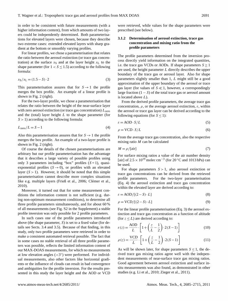
For linear profiles, we chose a parameterisation that relatesthe ratio between the aerosol extinction (or trace gas concen-tration) at the surfacexS and at the layer heightxL to theshape parameter (for 1< S ≤ 1.5) according to the followingformula:
xS/xL = (1.5−S) ·2 (3)
This parameterisation assures that forS → 1 the profilemerges the box profile. An example of a linear profile isshown in Fig. 2 (right).
For the two-layer profile, we chose a parameterisation thatrelates the ratio between the height of the near-surface layerwith zero aerosol extinction (or trace gas concentration)Lzeroand the (total) layer heightL to the shape parameter (forS > 1) according to the following formula:
Lzero/L = S −1 (4)
Also this parameterisation assures that forS → 1 the profilemerges the box profile. An example of a two-layer profile isshown in Fig. 2 (right).
Of course the details of the chosen parameterisations arearbitrary but our profile parameterisation has the advantagethat it describes a large variety of possible profiles usingonly 3 parameters including “box” profiles (S = 1), quasi-exponential profiles (S → 0), or profiles with an elevatedlayer (S > 1). However, it should be noted that this simpleparameterisation cannot describe more complex situationslike e.g. multiple layers (Frieß et al., 2006; Clemer et al.,2010).
Moreover, it turned out that for some measurement con-ditions the information content is not sufficient (e.g. dur-ing non-optimum measurement conditions), to determine allthree profile parameters simultaneously, and for about 60 %of all measurements (see Fig. S2 in the Supplement) a stableprofile inversion was only possible for 2 profile parameters.
In such cases one of the profile parameters introducedabove (the shape parameter,S) is set to a fixed value (for de-tails see Sects. 3.4 and 3.5). Because of that finding, in thisstudy, only two profile parameters were retrieved in order tomake a consistent automated retrieval possible. The fact thatin some cases no stable retrieval of all three profile parame-ters was possible, reflects the limited information content ofour MAX-DOAS measurements, for which no measurementsat low elevation angles (<3◦) were performed. For individ-ual measurements, also other factors like horizontal gradi-ents or the influence of clouds can result in bad convergenceand ambiguities for the profile inversion. For the results pre-sented in this study the layer height and the AOD or VCD
were retrieved, while values for the shape parameters wereprescribed (see below).
3.1.2 Determination of aerosol extinction, trace gasconcentration and mixing ratio from theprofile parameters
The profile parameters determined from the inversion pro-cess directly yield information on the integrated quantities,i.e. the trace gas VCDs or AODs. If shape parametersS ≥ 1are used, the height parameterL directly describes the upperboundary of the trace gas or aerosol layer. Also for shapeparameters slightly smaller than 1,L might still be a goodapproximation of the upper boundary of the aerosol or tracegas layer (for values ofS � 1, however, a correspondinglylarge fraction (1− S) of the total trace gas or aerosol amountis located aboveL).
From the derived profile parameters, the average trace gasconcentration,ρ, or the average aerosol extinction,ε, withinthe aerosol or trace gas layer can be derived according to thefollowing equations (forS ≤ 1):
ε = AOD ·S/L (5)
ρ = VCD ·S/L (6)
From the average trace gas concentration, also the respectivemixing ratioM can be calculated
M = ρ/[air] (7)
For surface mixing ratios a value of the air number density[air] of 2.5× 10¹⁹ molec cm−3 (for 20◦C and 1013 hPa) canbe used.
For shape parametersS > 1, also aerosol extinction ortrace gas concentrations can be derived from the retrievedprofile parameters. For the two-layer parameterisation(Eq. 4) the aerosol extinction and trace gas concentrationwithin the elevated layer are derived according to:
ε = AOD/[(2−S) ·L] (8)
ρ = VCD/[(2−S) ·L] (9)
For the linear profile parameterisation (Eq. 3) the aerosol ex-tinction and trace gas concentration as a function of altitude(for z ≤ L) are derived according to:
ε(z) =AOD
L·
[1+
(z
L−
1
2
)·2(S −1)
](10)
ρ(z) =VCD
L·
[1+
(z
L−
1
2
)·2(S −1)
](11)
As will be shown later, for shape parametersS ≤ 1, the de-rived trace gas mixing ratios agree well with the indepen-dent measurements of near-surface trace gas mixing ratios.Good agreement between aerosol extinction and surface in-situ measurements was also found, as demonstrated in otherstudies (e.g. Li et al., 2010; Zieger et al., 2011).
www.atmos-meas-tech.net/4/2685/2011/ Atmos. Meas. Tech., 4, 2685–2715, 2011
2692 T. Wagner et al.: Tropospheric trace gas and aerosol profiles from MAX DOAS
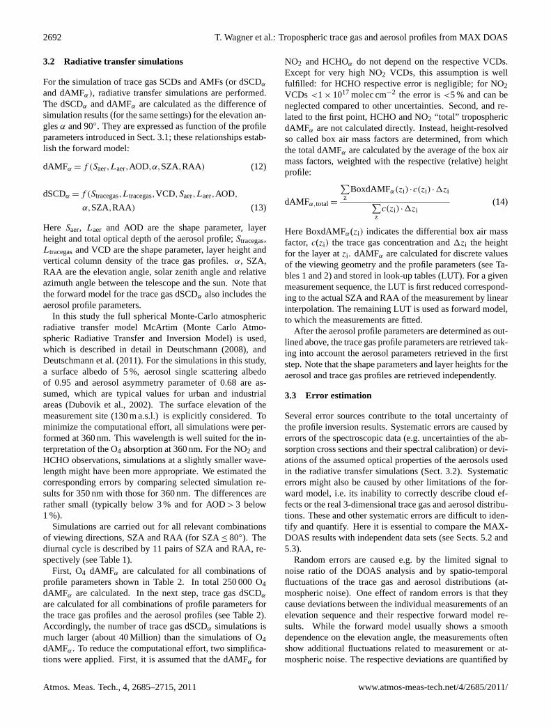
3.2 Radiative transfer simulations
For the simulation of trace gas SCDs and AMFs (or dSCDα
and dAMFα), radiative transfer simulations are performed.The dSCDα and dAMFα are calculated as the difference ofsimulation results (for the same settings) for the elevation an-glesα and 90◦. They are expressed as function of the profileparameters introduced in Sect. 3.1; these relationships estab-lish the forward model:
dAMFα = f (Saer,Laer,AOD,α,SZA,RAA) (12)
dSCDα = f (Stracegas,Ltracegas,VCD,Saer,Laer,AOD,
α,SZA,RAA) (13)
Here Saer, Laer and AOD are the shape parameter, layerheight and total optical depth of the aerosol profile;Stracegas,Ltracegasand VCD are the shape parameter, layer height andvertical column density of the trace gas profiles.α, SZA,RAA are the elevation angle, solar zenith angle and relativeazimuth angle between the telescope and the sun. Note thatthe forward model for the trace gas dSCDα also includes theaerosol profile parameters.
In this study the full spherical Monte-Carlo atmosphericradiative transfer model McArtim (Monte Carlo Atmo-spheric Radiative Transfer and Inversion Model) is used,which is described in detail in Deutschmann (2008), andDeutschmann et al. (2011). For the simulations in this study,a surface albedo of 5 %, aerosol single scattering albedoof 0.95 and aerosol asymmetry parameter of 0.68 are as-sumed, which are typical values for urban and industrialareas (Dubovik et al., 2002). The surface elevation of themeasurement site (130 m a.s.l.) is explicitly considered. Tominimize the computational effort, all simulations were per-formed at 360 nm. This wavelength is well suited for the in-terpretation of the O4 absorption at 360 nm. For the NO2 andHCHO observations, simulations at a slightly smaller wave-length might have been more appropriate. We estimated thecorresponding errors by comparing selected simulation re-sults for 350 nm with those for 360 nm. The differences arerather small (typically below 3 % and for AOD> 3 below1 %).
Simulations are carried out for all relevant combinationsof viewing directions, SZA and RAA (for SZA≤ 80◦). Thediurnal cycle is described by 11 pairs of SZA and RAA, re-spectively (see Table 1).
First, O4 dAMFα are calculated for all combinations ofprofile parameters shown in Table 2. In total 250 000 O4dAMFα are calculated. In the next step, trace gas dSCDα
are calculated for all combinations of profile parameters forthe trace gas profiles and the aerosol profiles (see Table 2).Accordingly, the number of trace gas dSCDα simulations ismuch larger (about 40 Million) than the simulations of O4dAMFα. To reduce the computational effort, two simplifica-tions were applied. First, it is assumed that the dAMFα for
NO2 and HCHOα do not depend on the respective VCDs.Except for very high NO2 VCDs, this assumption is wellfulfilled: for HCHO respective error is negligible; for NO2VCDs <1× 10¹⁷ molec cm−2 the error is<5 % and can beneglected compared to other uncertainties. Second, and re-lated to the first point, HCHO and NO2 “total” troposphericdAMFα are not calculated directly. Instead, height-resolvedso called box air mass factors are determined, from whichthe total dAMFα are calculated by the average of the box airmass factors, weighted with the respective (relative) heightprofile:
dAMFα,total=
∑z
BoxdAMFα(zi) ·c(zi) ·1zi∑z
c(zi) ·1zi(14)
Here BoxdAMFα(zi) indicates the differential box air massfactor, c(zi) the trace gas concentration and1zi the heightfor the layer atzi . dAMFα are calculated for discrete valuesof the viewing geometry and the profile parameters (see Ta-bles 1 and 2) and stored in look-up tables (LUT). For a givenmeasurement sequence, the LUT is first reduced correspond-ing to the actual SZA and RAA of the measurement by linearinterpolation. The remaining LUT is used as forward model,to which the measurements are fitted.
After the aerosol profile parameters are determined as out-lined above, the trace gas profile parameters are retrieved tak-ing into account the aerosol parameters retrieved in the firststep. Note that the shape parameters and layer heights for theaerosol and trace gas profiles are retrieved independently.
3.3 Error estimation
Several error sources contribute to the total uncertainty ofthe profile inversion results. Systematic errors are caused byerrors of the spectroscopic data (e.g. uncertainties of the ab-sorption cross sections and their spectral calibration) or devi-ations of the assumed optical properties of the aerosols usedin the radiative transfer simulations (Sect. 3.2). Systematicerrors might also be caused by other limitations of the for-ward model, i.e. its inability to correctly describe cloud ef-fects or the real 3-dimensional trace gas and aerosol distribu-tions. These and other systematic errors are difficult to iden-tify and quantify. Here it is essential to compare the MAX-DOAS results with independent data sets (see Sects. 5.2 and5.3).
Random errors are caused e.g. by the limited signal tonoise ratio of the DOAS analysis and by spatio-temporalfluctuations of the trace gas and aerosol distributions (at-mospheric noise). One effect of random errors is that theycause deviations between the individual measurements of anelevation sequence and their respective forward model re-sults. While the forward model usually shows a smoothdependence on the elevation angle, the measurements oftenshow additional fluctuations related to measurement or at-mospheric noise. The respective deviations are quantified by
Atmos. Meas. Tech., 4, 2685–2715, 2011 www.atmos-meas-tech.net/4/2685/2011/

T. Wagner et al.: Tropospheric trace gas and aerosol profiles from MAX DOAS 2693
Table 1. Selected times of the day and corresponding solar zenith angles (SZA) and relative azimuth angles (RAA) angles, for whichradiative transfer simulations are performed.
Time of05:57 06:55 07:55 09:07 09:53 10:31 12:46 13:31 14:41 15:42 16:41
the day (UTC)
SZA 80◦ 70◦ 60◦ 50◦ 45◦ 42◦ 45◦ 50◦ 60◦ 70◦ 80◦
RAA (S) −90◦−80◦
−67◦−46◦
−29◦−5◦ 19◦ 36◦ 56◦ 70◦ 81◦
RAA (W) −155◦ −145◦ −132◦ −111◦ −94◦−70◦
−46◦−29◦
−9◦ 5◦ 16◦
RAA (N) 90◦ 100◦ 113◦ 134◦ 151◦ 175◦ 199◦ 216◦ 236◦ 250◦ 261◦
Table 2. Selected elevation angles and profile parameters, for which air mass factors for O4, HCHO, and NO2 were calculated. O4 dAMFα
were calculated for all possible aerosol profiles. Trace gas dAMFα (NO2 and HCHO) were calculated for all combinations of aerosol andtrace gas profiles. For each case shown in Table 1, all combinations described in Table 2 were considered for the radiative transfer modelling.No clouds were included in the simulations.
QuantityNumber
Selected valuesof cases
Elevation angles 5 3◦, 6◦, 10◦, 18◦, 90◦
AOD 10 0.05, 0.1, 0.2, 0.3, 0.5, 0.7, 1.0, 1.5, 2.0, 3.0Aerosol layer heightLaer 14 20 m, 100 m, 200 m, 300 m, 500 m, 700 m, 1000 m, 1200 m, 1500 m, 1750 m, 2000 m, 2500 m, 3000 m, 5000 mAerosol shape parameterSaer 11 0.1, 0.2, 0.3, 0.4, 0.5, 0.7, 1.0, 1.1, 1.2, 1.5, 1.8Trace gas layer heightLtracegas 14 20 m, 100 m, 200 m, 300 m, 500 m, 700 m, 1000 m, 1200 m, 1500 m, 1750 m, 2000 m, 2500 m, 3000 m, 5000 mTrace gas shape parameterStracegas 11 0.1, 0.2, 0.3, 0.4, 0.5, 0.7, 1.0, 1.1, 1.2, 1.5, 1.8
the residual sum of squares (RSS) between the measurementsand the forward model:
RSS=
n∑i=1
[yi −f (xi)]2 (15)
In the following, retrieval results with large deviations be-tween measurements and forward model (RSS> 0.05) aregenerally skipped.
In addition to the RSS between measurements and forwardmodel, inversion errors can also be quantified from the fitprocess itself (see also Li et al., 2010) taking into account thesensitivity of the measured quantities with respect to varia-tions of the profile parameters. Errors determined in this wayin this study are representative for a confidence interval of95 %. We found that the errors determined in this way arelargely proportional to the RSS, which indicates that theytypically represent random errors of the spectral retrievaland/or “atmospheric noise”.
From a linear fit of these errors versus the correspondingvalues of the profile parameters, the typical relative errorsare determined. To this regression line, a constant value issubsequently added to assure that for the smallest retrievedvalues the linear parameterisation still matches the respectiveuncertainties. Thus this error estimate represents an upperlimit. The error parameterisations for the different retrievedquantities are summarised in Table 3; they were used for thecorrelation analyses presented in Sect. 5.2. Also shown in
Table 3 are the mean relative errors. They range from about9 % for the NO2 mixing ratio to 71 % for the aerosol layerheight.
3.4 Aerosol inversion
In the first step of the trace gas profile inversion, theaerosol extinction profile is determined from the measuredO4 DAMF (Eq. 2). Since MAX-DOAS spectra are analysedagainst a fixed Fraunhofer reference spectrum (see Sect. 2.3),the retrieved O4 DAMF contain not only the difference com-pared to the zenith spectrum of the same elevation sequence(as needed for the inversion), but also a SZA dependent off-set. To remove this offset, the O4 DAMF for the 90◦ eleva-tion spectrum of the selected elevation sequence is subtractedfrom the O4 DAMF for all other (slant) elevation angles ofthis sequence to yield the respective dAMFα.
In this study only two profile parameters (AOD and layerheight L) are varied during the fitting process, while theshape parameterS is set to a fixed value.
To minimise the effect of the initial values on the inver-sion, we applied the following fitting procedure: in a firststep the optimum AOD is determined in individual fits (ac-cording to the minimum RSS) for the discrete values of theaerosol layer height used for the radiative transfer simula-tions (see Table 2). In a second step a low order polyno-mial as function of the aerosol layer height is fitted to the
www.atmos-meas-tech.net/4/2685/2011/ Atmos. Meas. Tech., 4, 2685–2715, 2011
2694 T. Wagner et al.: Tropospheric trace gas and aerosol profiles from MAX DOAS
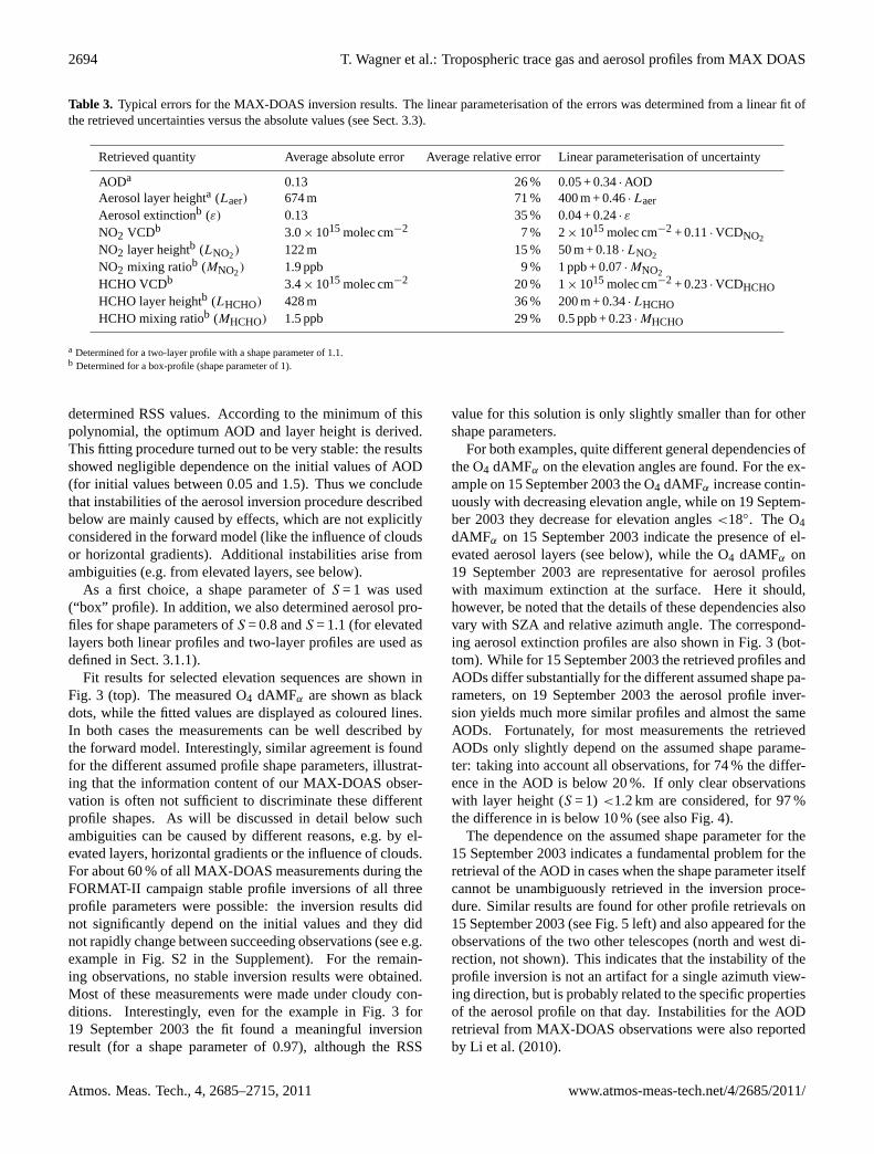
Table 3. Typical errors for the MAX-DOAS inversion results. The linear parameterisation of the errors was determined from a linear fit ofthe retrieved uncertainties versus the absolute values (see Sect. 3.3).
Retrieved quantity Average absolute error Average relative error Linear parameterisation of uncertainty
AODa 0.13 26 % 0.05 + 0.34· AODAerosol layer heighta (Laer) 674 m 71 % 400 m + 0.46· LaerAerosol extinctionb (ε) 0.13 35 % 0.04 + 0.24· εNO2 VCDb 3.0× 10¹⁵molec cm−2 7 % 2× 10¹⁵molec cm−2 + 0.11· VCDNO2
NO2 layer heightb (LNO2) 122 m 15 % 50 m + 0.18· LNO2
NO2 mixing ratiob (MNO2) 1.9 ppb 9 % 1 ppb + 0.07· MNO2
HCHO VCDb 3.4× 10¹⁵molec cm−2 20 % 1× 10¹⁵molec cm−2 + 0.23· VCDHCHOHCHO layer heightb (LHCHO) 428 m 36 % 200 m + 0.34· LHCHOHCHO mixing ratiob (MHCHO) 1.5 ppb 29 % 0.5 ppb + 0.23· MHCHO
a Determined for a two-layer profile with a shape parameter of 1.1.b Determined for a box-profile (shape parameter of 1).
determined RSS values. According to the minimum of thispolynomial, the optimum AOD and layer height is derived.This fitting procedure turned out to be very stable: the resultsshowed negligible dependence on the initial values of AOD(for initial values between 0.05 and 1.5). Thus we concludethat instabilities of the aerosol inversion procedure describedbelow are mainly caused by effects, which are not explicitlyconsidered in the forward model (like the influence of cloudsor horizontal gradients). Additional instabilities arise fromambiguities (e.g. from elevated layers, see below).
As a first choice, a shape parameter ofS = 1 was used(“box” profile). In addition, we also determined aerosol pro-files for shape parameters ofS = 0.8 andS = 1.1 (for elevatedlayers both linear profiles and two-layer profiles are used asdefined in Sect. 3.1.1).
Fit results for selected elevation sequences are shown inFig. 3 (top). The measured O4 dAMFα are shown as blackdots, while the fitted values are displayed as coloured lines.In both cases the measurements can be well described bythe forward model. Interestingly, similar agreement is foundfor the different assumed profile shape parameters, illustrat-ing that the information content of our MAX-DOAS obser-vation is often not sufficient to discriminate these differentprofile shapes. As will be discussed in detail below suchambiguities can be caused by different reasons, e.g. by el-evated layers, horizontal gradients or the influence of clouds.For about 60 % of all MAX-DOAS measurements during theFORMAT-II campaign stable profile inversions of all threeprofile parameters were possible: the inversion results didnot significantly depend on the initial values and they didnot rapidly change between succeeding observations (see e.g.example in Fig. S2 in the Supplement). For the remain-ing observations, no stable inversion results were obtained.Most of these measurements were made under cloudy con-ditions. Interestingly, even for the example in Fig. 3 for19 September 2003 the fit found a meaningful inversionresult (for a shape parameter of 0.97), although the RSS
value for this solution is only slightly smaller than for othershape parameters.
For both examples, quite different general dependencies ofthe O4 dAMFα on the elevation angles are found. For the ex-ample on 15 September 2003 the O4 dAMFα increase contin-uously with decreasing elevation angle, while on 19 Septem-ber 2003 they decrease for elevation angles<18◦. The O4dAMFα on 15 September 2003 indicate the presence of el-evated aerosol layers (see below), while the O4 dAMFα on19 September 2003 are representative for aerosol profileswith maximum extinction at the surface. Here it should,however, be noted that the details of these dependencies alsovary with SZA and relative azimuth angle. The correspond-ing aerosol extinction profiles are also shown in Fig. 3 (bot-tom). While for 15 September 2003 the retrieved profiles andAODs differ substantially for the different assumed shape pa-rameters, on 19 September 2003 the aerosol profile inver-sion yields much more similar profiles and almost the sameAODs. Fortunately, for most measurements the retrievedAODs only slightly depend on the assumed shape parame-ter: taking into account all observations, for 74 % the differ-ence in the AOD is below 20 %. If only clear observationswith layer height (S = 1) <1.2 km are considered, for 97 %the difference in is below 10 % (see also Fig. 4).
The dependence on the assumed shape parameter for the15 September 2003 indicates a fundamental problem for theretrieval of the AOD in cases when the shape parameter itselfcannot be unambiguously retrieved in the inversion proce-dure. Similar results are found for other profile retrievals on15 September 2003 (see Fig. 5 left) and also appeared for theobservations of the two other telescopes (north and west di-rection, not shown). This indicates that the instability of theprofile inversion is not an artifact for a single azimuth view-ing direction, but is probably related to the specific propertiesof the aerosol profile on that day. Instabilities for the AODretrieval from MAX-DOAS observations were also reportedby Li et al. (2010).
Atmos. Meas. Tech., 4, 2685–2715, 2011 www.atmos-meas-tech.net/4/2685/2011/

T. Wagner et al.: Tropospheric trace gas and aerosol profiles from MAX DOAS 2695
15 September 2003, 12:00 19 September 2003, 8:00
0
0.2
0.4
0.6
0.8
1
0 5 10 15 20Elevation angle [°]
O4 d
AM
F αReihe1Reihe2Reihe9Reihe8Reihe3
MeasurementS = 1.1S = 1.0S = 0.8S = 1.1 (linear)
0
0.2
0.4
0.6
0.8
1
0 5 10 15 20Elevation angle [°]
O4 d
AMF α
Reihe1Reihe2Reihe9Reihe8Reihe3
MeasurementS = 1.1S = 1.0S = 0.8S = 1.1 (linear)
S = 1.1 AOD: 0.40S = 1.0 AOD: 0.85S = 0.8 AOD: 1.28S = 1.1 lin AOD: 1.28
S = 1.1 AOD: 0.61S = 1.0 AOD: 0.77
S = 1.1 lin AOD: 0.78S = 0.8 AOD: 0.73
S = 1.1 AOD: 0.40S = 1.0 AOD: 0.85
S = 1.1 lin AOD: 1.28
S = 1.1 AOD: 0.61S = 1.0 AOD: 0.77
S = 1.1 lin AOD: 0.78S = 0.8 AOD: 1.28 S = 0.8 AOD: 0.73
Fig. 3 Top: comparison of measured O4 dAMFα (black dots) to the results of the forward model (coloured lines) for the southern telescope. The different colours indicate fit results for different shape parameters. The error bars indicate the errors of the spectral analysis. Both observations were made under clear sky conditions. Bottom: Resulting aerosol extinction profiles retrieved from the O4 dAMFα.
39
Fig. 3. Top: comparison of measured O4 dAMFα (black dots) to the results of the forward model (coloured lines) for the southern telescope.The different colours indicate fit results for different shape parameters. The error bars indicate the errors of the spectral analysis. Bothobservations were made under clear sky conditions. Bottom: resulting aerosol extinction profiles retrieved from the O4 dAMFα .
In Fig. 5 the retrieved layer heights and extinction coeffi-cients for both days are also shown. It is interesting to notethat the rapid jumps of the AOD for shape parametersS ≤ 1or for the linear profile withS = 1.1 are closely correlated tosimilar rapid changes of the layer heightL (Fig. 5 middle).As a consequence the aerosol extinction (Eqs. 5, 8, 10) ismuch less dependent on the profile shape than the AOD (bot-tom panel of Fig. 5). Also the uncertainties of the retrievedaerosol extinction are much smaller than those of the AODsor layer heights.
On 19 September 2003 a different behaviour compared to15 September is found: the extinction coefficient dependsmore strongly on the assumed profile shape than the AOD(see Fig. 5 right). Also the uncertainties of the aerosol ex-tinction is much larger indicating that on that day a two-layer profile with shape parameter of 1.1 might not be a goodchoice for the determination of the aerosol extinction. Hereit should be noted, that the aerosol extinction determined forthe two layer profile with zero values at the surface can bydefinition not be representative for the actual aerosol extinc-
tion at the surface (the data in Fig. 5 is shown again in theSupplement (Fig. S3), but with the uncertainties displayedfor the retrieval assuming a box profile).
We investigated possible reasons for the instabilities ofthe aerosol profile inversion and the dependence of the AODon the profile shape. One hypothesis is that on 15 Septem-ber 2003 an elevated aerosol layer might have been present.An indication for this hypothesis is found in the results forshape parametersS > 1. If profiles for an elevated aerosollayer are used (either a linear profile or a two-layer profile),the diurnal variation of the AOD shows a much smootherbehaviour. The most consistent temporal variation is foundfor a two-layer parameterisation (assuming a layer with zeroaerosol extinction at the surface).
We further tested our hypothesis of an elevated layer byperforming radiative transfer simulations for different as-sumed aerosol extinction profiles (see Fig. 6). It turned outthat for the elevation angles used in this study (≥3◦, indicatedby the black arrows), the simulations for a two-layer profilewith shape parameter of 1.1 (andL = 1, AOD = 0.3) can be
www.atmos-meas-tech.net/4/2685/2011/ Atmos. Meas. Tech., 4, 2685–2715, 2011

2696 T. Wagner et al.: Tropospheric trace gas and aerosol profiles from MAX DOAS
shape parameter: 0.8 shape parameter: S = 1.0
0
0.5
1
1.5
2
2.5
3
3.5
0 0.2 0.4 0.6 0.8 10
0.5
1
1.5
2
2.5
0 0.2 0.4 0.6 0.8 1OD elevated layer (S = 1.1)
OD
box
pro
file
(S =
1.0
)
OD elevated layer (S = 1.1)
OD
pro
file
(S =
0.8
)
layer height (s = 0.8) > 1.0 km layer height (s = 0.8) < 1.0 km
layer height (s = 1.0) > 1.2 km layer height (s = 1.0) < 1.2 km
y = 1.22x - 0.016r2 = 0.98
y = 1.17x - 0.016r2 = 0.99
Fig. 4 Comparison of MAX-DOAS AODs retrieved for different shape parameters S for clear days. The AOD for S = 0.8 (left) and S = 1.0 (right) is plotted versus the AOD retrieved for S = 1.1. Good agreement is found for retrieved layer heights below 1.2 km (S = 0.8) and 1.2 km (S = 1.0), respectively.
40
Fig. 4. Comparison of MAX-DOAS AODs retrieved for different shape parametersS for clear days. The AOD forS = 0.8 (left) andS = 1.0(right) is plotted versus the AOD retrieved forS = 1.1. Good agreement is found for retrieved layer heights below 1.2 km (S = 0.8) and 1.2 km(S = 1.0), respectively.
15 September 2003 19 September 2003
0
0.5
1
1.5
2
5:00 7:00 9:00 11:00 13:00 15:00Time
Aero
sol O
D
Reihe3Reihe5Reihe6Reihe1AOT_350
S = 0.8S = 1.0S = 1.1S = 1.1 (linear)AERONET
0
0.5
1
1.5
2
5:00 7:00 9:00 11:00 13:00 15:00Time
Aer
osol
OD
Reihe3Reihe5Reihe6Reihe1AOT_350
S = 0.8S = 1.0S = 1.1S = 1.1 (linear)AERONET
0
1000
2000
3000
4000
5000
5:00 7:00 9:00 11:00 13:00 15:00Time
Laye
r hei
ght [
m]
Reihe3Reihe5Reihe6Reihe1
S = 0.8S = 1.0S = 1.1S = 1.1 (li )
0
1000
2000
3000
4000
5000
5:00 7:00 9:00 11:00 13:00 15:00Time
Laye
r hei
ght [
m]
Reihe3Reihe5Reihe6Reihe2
S = 0.8S = 1.0S = 1.1S = 1.1 (linear)
0
0.5
1
1.5
2
2.5
5:00 7:00 9:00 11:00 13:00 15:00Time
Aer
osol
ext
inct
ion
[1/k
m]
Reihe3Reihe5Reihe4Reihe1
S = 0.8S = 1.0S = 1.1S = 1.1 (linear)
0
0.5
1
1.5
2
2.5
5:00 7:00 9:00 11:00 13:00 15:00Time
Aero
sol e
xtin
ctio
n [1
/km
]
Reihe3Reihe5Reihe4Reihe2
S = 0.8S = 1.0S = 1.1S = 1.1 (linear)
Fig. 5 Diurnal variation of the AOD (top), layer height L (middle) and aerosol extinction ε (bottom) for different shape parameters (southern telescope). For comparison, also the AOD from sun photometer measurements (AERONET) at Ispra are shown (dark blue line). Except the early morning of 15 September 2003 (before about 7:00), both days were cloud free. Error bars (for 95% confidence intervals) are determined within the inversion procedure; they are exemplarily shown for the retrieval assuming an elevated layer (two-layer profile). A similar figure, but with error bars for box profile inversion is shown in the supplement (Fig. S3).
41
Fig. 5. Diurnal variation of the AOD (top), layer heightL (middle) and aerosol extinctionε (bottom) for different shape parameters (southerntelescope). For comparison, also the AOD from sun photometer measurements (AERONET) at Ispra are shown (dark blue line). Except theearly morning of 15 September 2003 (before about 07:00), both days were cloud free. Error bars (for 95 % confidence intervals) aredetermined within the inversion procedure; they are exemplarily shown for the retrieval assuming an elevated layer (two-layer profile). Asimilar figure, but with error bars for box profile inversion is shown in the Supplement (Fig. S3).
Atmos. Meas. Tech., 4, 2685–2715, 2011 www.atmos-meas-tech.net/4/2685/2011/

T. Wagner et al.: Tropospheric trace gas and aerosol profiles from MAX DOAS 2697
well reproduced by the simulations for a box-profile (shapeparameter of 1), but with larger values forL and AOD (4 kmand 1, respectively). Also the simulations for a linear profilecan match the results for the two-layer profile. This find-ing confirms the hypothesis that in the presence of elevatedaerosol layers, no unambiguous profile inversion might bepossible for the elevation angles used in this study.
The ambiguity demonstrated in Fig. 6 can explain the ob-servations on 15 September 2003 (Fig. 5 left), for which in-creased AOD are often found with simultaneously enhancedlayer height. They also indicate that if additional viewingangles at low elevation were included in the MAX-DOASobservations, the ambiguity of the profile retrieval could beeffectively reduced.
It should be noted that a profile with zero aerosol extinc-tion at the surface is probably not very reasonable close tostrong emission sources like for our measurements (see dis-cussion in Sect. 3.1.1). Nevertheless, the smooth diurnalvariation found for this profile parameterisation indicates thatstrong vertical gradients of the aerosol extinction probablyexist close to the surface, which are better described by thetwo-layer profile than by the other profile parameterisations.
To deal with the problem of underdetermination of theaerosol profile, we chose a pragmatic solution by simply us-ing a shape parameter of 1.1 (two layer profile) for the de-termination of the AOD. By this choice, stable results forthe AOD are obtained for all days (results for one day areshown in Fig. 5 left). But of course, this choice has alsodisadvantages: for many days (without elevated profiles) weuse an assumption which is obviously wrong. As a conse-quence, the retrieved AOD is often smaller than for shapeparametersS ≤ 1 (see Fig. 5 right), but fortunately this un-derestimation is usually small: for 74 % of all observationsit is less than 20 %; for 97 % of clear observations with layerheight (S = 1) <1.2 km the difference in the AOD is below10 % (see also Fig. 4). Another disadvantage is that the re-trieved layer height for a shape parameter ofS = 1.1 is sys-tematically lower (typically by a factor of about 2) than fora shape parameter of 1 (Fig. 5, middle). There is probablyno simple explanation for this finding, but the fact thatL1.1is systematically smaller thanL1.0 is also supported by theresults of Fig. 6 (and Fig. S4 in the Supplement), where theO4 DSCDs for profiles withS = 1 andL = 1 km agree withthose for profiles withS > 1 andL > 1 km.
Note that the results for the aerosol layer height presentedin the following sections were retrieved for a shape parameterof 1.1, and were subsequentially multiplied by a factor of twoin order to be representative for the true aerosol layer height.As will be shown in Sect. 5.3, the aerosol layer heights de-termined in this way agree reasonably well with aerosol con-centration profiles from aircraft measurements.
Also, for shape parametersS < 1 systematically lowerlayer heights are retrieved than forS = 1. This has to be ex-pected, because for these S-values a substantial part of theaerosol load is located above the “aerosol layer”.
0
0.2
0.4
0.6
0.8
1
1.2
1.4
1.6
1.8
1 10Elevation angle [°]
O4 d
AM
F α
100
Reihe2Reihe3Reihe4Reihe6
0 - 4km, (S = 1), OD 10 - 1km, (S = 1), OD 0.30.1 - 1km (S = 1.1), OD 0.3linear increase by 2/3 (S = 1.35), OD 0.3
Fig. 6 Simulated O4 dAMFα for different assumed profile shapes. Besides the elevation angles used in this study (indicated by the black arrows) the calculations also include further elevation angles, especially below 3°. Calculations are preformed for SZA of 30° and a relative azimuth angle of 0°.
42
Fig. 6. Simulated O4 dAMFα for different assumed profile shapes.Besides the elevation angles used in this study (indicated by theblack arrows) the calculations also include further elevation angles,especially below 3◦. Calculations are preformed for SZA of 30◦
and a relative azimuth angle of 0◦.
While for our measurements, an aerosol profile withS = 1.1 is probably an acceptable (pragmatic) choice for theretrieval of the AOD and layer height, it is not necessarily agood choice for other retrieved quantities. For example, asshown in Fig. 5, for shape parametersS ≤ 1 the retrieval ofthe aerosol extinction leads to much more consistent results.As will be shown below, the results of the trace gas inver-sions (especially for the trace gas VCD and layer height) arealso more realistic and consistent, if shape parametersS ≤ 1for the aerosol profile inversion are chosen.
The different choice of the shape parameterS for either theretrieval of AOD or the retrieval of trace gas profiles mightbe seen as an inconsistency. However, we think these choicesare well justified. As discussed above, the choice ofS > 1.1leads to more consistent results of the AOD than the use ofS ≤ 1. However, if the aerosol extinction profiles forS = 1.1were also used as input for the trace gas profile inversion,a particular problem occurs: the aerosol extinction close tothe surface would be systematically underestimated in mostcases, while the maximum trace gas concentrations are typ-ically located at these altitudes. To avoid this problem, weuse aerosol extinction profiles retrieved for a shape parame-ter S ≤ 1. Even if in some cases the AOD (and the aerosollayer height) would be overestimated, the aerosol extinctionclose to the surface will very probably be more correct thanthat for aerosol retrievals withS = 1.1.
3.5 Trace gas inversion (NO2 and HCHO)
The inversion of the trace gas profiles (second step) is per-formed in a similar way to the aerosol inversion. First theDSCDs for the 90◦ elevation angles are subtracted from theDSCDs of the lower elevation angles of the same sequenceto yield the respective dSCDα. In the next step the tracegas dSCDα are divided by the dSCDα for an elevation angle
www.atmos-meas-tech.net/4/2685/2011/ Atmos. Meas. Tech., 4, 2685–2715, 2011

2698 T. Wagner et al.: Tropospheric trace gas and aerosol profiles from MAX DOAS
α = 10◦ of the same elevation sequence (in principle anyother elevation angle could be used as well). This normalisa-tion is performed to simplify the fitting process of the tracegas inversion. In contrast to the aerosol inversion, where theO4 DAMF depend not only on the relative profile shape butalso on the absolute value of the AOD, the dAMFα for NO2and HCHO do not depend on the absolute value of VCD, be-cause their atmospheric absorptions are weak (OD typically<0.1). Thus, the profile inversion for NO2 and HCHO canbe reduced to the determination of the relative profile shapes(also see Sinreich et al., 2005).
Before the fit to the normalised trace gas dSCDα, a similarnormalisation of the dAMFα of the forward model is applied.From the fit between the measurements and the forwardmodel, the (relative) profile shape (layer height, and shapeparameter) and the corresponding dAMFα are obtained. Thisis possible because of the unique relationship between nor-malised dAMF and the absolute dAMF, from which the nor-malised dAMF were calculated. From the dAMFα and themeasured trace gas dSCDα the VCDs for the individual ele-vation angles are calculated:
VCDα=dSCDα
dAMFα
(16)
Finally, the average of the VCDs for the different elevationsequences is calculated. From the VCD, the layer height,and the shape parameter the average trace gas concentrationor mixing ratio is calculated according to Eqs. (6, 7, 9, and11). Like the aerosol inversion, in some cases the trace gasinversion has no stable convergence, and thus, the shape pa-rameterS, is prescribed. Thus only the layer heightL andthe VCD were determined independently by the fit.
In Fig. 7 exemplary fit results of the forward model tothe measured (normalised) dSCDα of NO2 and HCHO areshown. Like the aerosol inversion, similar agreement for thedifferent shape parameters is found. The VCDs retrieved forshape parameters≤1 show rather good agreement, but forshape parameters>1 (elevated layers), systematically lowerVCDs are obtained. However, in contrast to the aerosol in-version, the results of the trace gas inversions did not showinstabilities like those in Fig. 5 (left column). Thus in thefollowing, only trace gas results for shape parameters≤1 arepresented. The better convergence of the trace gas VCDs(compared to the AOD) is probably caused by fact that en-hanced concentrations of NO2 and HCHO are usually con-fined to the lowest atmospheric layers, while the atmosphericscale height of O4 is about 4 km.
In Fig. 8 the diurnal variations of the retrieved trace gasresults (VCD, layer height and mixing ratio) are presentedfor 19 September 2003. For comparison, the mixing ratiosof the independent measurements (LP-DOAS and Hantzsch)are also shown. In general, the HCHO layers (and their un-certainties) are higher than those of NO2.
The trace gas VCDs from the profile inversion are com-pared to the respective VCDs calculated by the so called ge-ometric approximation (A. Richter, personal communication,2005; Brinksma et al., 2008). In this study we used the mea-surements at elevation angles of 18◦ and 90◦ for the determi-nation of the “geometric” VCD:
VCDgeo=dSCD18◦
dAMF18◦
=dSCD18◦
1/
sin(18◦) − 1(17)
While the trace gas VCDs from the profile inversions assum-ing different shape parameters show very good agreement,the geometric VCDs are mostly smaller than the VCDs fromthe profile inversions (especially for periods with high tracegas VCDs). These differences are most probably caused bythe neglect of scattering processes in the calculation of thegeometric VCD. The systematic deviations between the ge-ometric VCD and the VCDs from the profile inversion arefurther investigated in Sect. 5.2.4.
As pointed out before, the results of the aerosol inversionare used as input for the trace gas profile inversion. Thus thequestion arises, which aerosol shape parameterSaershould beused in the first step of the trace gas retrievals. To answer thisquestion we compared trace gas results for different assumedaerosol shape parametersSaer (for simplicity, the shape pa-rameter for the trace gas inversionStracegaswas set to 1). Theresults are presented in Fig. 9. While the trace gas mixingratios are only slightly affected by different choices ofSaer,the trace gas VCDs and layer heights for differentSaer showlarge differences. Especially forSaer> 1 they deviate sys-tematically from the results forSaer≤ 1. The reason for thisfinding is not clear, but is probably related to the fact thatfor aerosol shape parametersSaer> 1 the aerosol extinctionclose to the ground is systematically underestimated. This isthe layer where usually the highest trace gas concentrationsoccur. Fortunately, the trace gas mixing ratios depend littleon the assumed aerosol shape parameter.
4 Influence of clouds on MAX-DOAS observations
Like aerosols, clouds also strongly affect the atmospheric ra-diative transfer and can have a large effect on MAX-DOASobservations and the profile retrievals. Thus, the profile in-version for measurements at cloudy conditions is probablystrongly influenced by clouds. In this section the effects ofclouds on MAX-DOAS measurements are investigated. Firsta simple cloud classification algorithm is presented, whichis used to categorise the MAX-DOAS measurements duringthe FORMAT-II campaign into different classes. Based onthis classification scheme, the cloud effect on MAX-DOASresults can be empirically determined by comparison withindependent data. Cloud effects are also investigated usingradiative transfer simulations.
Atmos. Meas. Tech., 4, 2685–2715, 2011 www.atmos-meas-tech.net/4/2685/2011/

T. Wagner et al.: Tropospheric trace gas and aerosol profiles from MAX DOAS 2699
0
0.2
0.4
0.6
0.8
1
1.2
1.4
0 5 10 15 20Elevation angle [°]
dAM
F α ra
tio
(or
dS
CDα
ratio
)Reihe1Reihe2Reihe9Reihe8Reihe3
MeasurementS = 1.1S = 1.0S = 0.8S = 0.5
NO2
0
0.2
0.4
0.6
0.8
1
1.2
1.4
0 5 10 15 20Elevation angle [°]
dAM
F α ra
tio
(or
dS
CDα
ratio
)
Reihe1Reihe2Reihe9Reihe8Reihe3
MeasurementS = 1.1S = 1.0S = 0.8S = 0.5
HCHO
S: 0.5, L=183m, VCD=6.08 ⋅ 1016 molec/cm² S: 0.8, L=267m, VCD=5.67 ⋅ 1016 molec/cm² S: 1.0, L=320m, VCD=5.48 ⋅ 1016 molec/cm² S: 1.1, L=254m, VCD=5.09 ⋅ 1016 molec/cm²
S: 0.5, L=282m, VCD=2.23 ⋅ 1016 molec/cm² S: 0.8, L=445m, VCD=2.13 ⋅ 1016 molec/cm² S: 1.0, L=515m, VCD=2.01 ⋅ 1016 molec/cm² S: 1.1, L=350m, VCD=1.70 ⋅ 1016 molec/cm²
Fig. 7 Comparison of measured ratios of the NO2 and HCHO dSCDα (or dAMFα) relative to the 10° elevation (black dots) to the respective results of the forward model (coloured lines) for the southern telescope (19 September 2003, 8:00). The different colours indicate fit results for different profile shapes. The error bars indicate the errors of the spectral analysis.
43
Fig. 7. Comparison of measured ratios of the NO2 and HCHO dSCDα (or dAMFα) relative to the 10◦ elevation (black dots) to the respectiveresults of the forward model (coloured lines) for the southern telescope (19 September 2003, 08:00). The different colours indicate fit resultsfor different profile shapes. The error bars indicate the errors of the spectral analysis.
NO2 VCD HCHO VCD
0
1E+17
2E+17
3E+17
4E+17
5:00 7:00 9:00 11:00 13:00 15:00 17:00Time
NO
2 VC
D [m
olec
/cm
²] Reihe1Reihe2Reihe3Reihe4
S = 0.5S = 0.8S = 1.0'geometric VCD'
0.0E+00
5.0E+16
1.0E+17
1.5E+17
2.0E+17
5:00 7:00 9:00 11:00 13:00 15:00 17:00Time
HC
HO
VC
D [m
olec
/cm
²]
Reihe1Reihe2Reihe3Reihe4
S = 0.5S = 0.8S = 1.0'geometric VCD'
NO2 layer height HCHO layer height
0
500
1000
1500
2000
2500
3000
5:00 7:00 9:00 11:00 13:00 15:00 17:00Time
Laye
r hei
ght [
m]
Reihe1Reihe2Reihe3
S = 0.5S = 0.8S = 1.0
0
500
1000
1500
2000
2500
3000
5:00 7:00 9:00 11:00 13:00 15:00 17:00Time
Laye
r hei
ght [
m]
Reihe6
Reihe3
Reihe5
S = 0.5S = 0.8S = 1.0
NO2 mixing ratio HCHO mixing ratio
0
50
100
150
200
5:00 7:00 9:00 11:00 13:00 15:00 17:00Time
NO
2 mix
ing
ratio
[ppb
]
Reihe1Reihe2Reihe3 NO2_[ppb]
S = 0.5S = 0.8S = 1.0LP-DOAS
0
10
20
30
40
50
5:00 7:24 9:48 12:12 14:36 17:00Time
HC
HO
mix
ing
ratio
[ppb
] .
Reihe1Reihe2Reihe3 HCHO_[ppb]HCHO-PPB
S = 0.5S = 0.8S = 1.0LP-DOASHantzsch
Fig. 8 Diurnal variation of the inversion results for NO2 (left) and HCHO (right) for the southern telescope on 19 September 2003. In the top panel the trace gas VCDs, in the center panel the layer heights, and in the bottom panel the trace gas mixing ratios are shown. For comparison, also ‘geometric’ VCDs (see Eq. 17) and trace gas mixing rations obtained by independent measurements (LP-DOAS and Hantzsch) are shown. Error bars (for a 95% confidence interval) are determined from the inversion procedure; they are exemplarily shown for the retrieval assuming a box profile (S = 1.0).
44
Fig. 8. Diurnal variation of the inversion results for NO2 (left) and HCHO (right) for the southern telescope on 19 September 2003. Inthe top panel the trace gas VCDs, in the center panel the layer heights, and in the bottom panel the trace gas mixing ratios are shown.For comparison, also “geometric” VCDs (see Eq. 17) and trace gas mixing rations obtained by independent measurements (LP-DOAS andHantzsch) are shown. Error bars (for a 95 % confidence interval) are determined from the inversion procedure; they are exemplarily shownfor the retrieval assuming a box profile (S = 1.0).
www.atmos-meas-tech.net/4/2685/2011/ Atmos. Meas. Tech., 4, 2685–2715, 2011

2700 T. Wagner et al.: Tropospheric trace gas and aerosol profiles from MAX DOAS
0
1E+17
2E+17
3E+17
4E+17
5E+17
6E+17
7E+17
5:00 7:00 9:00 11:00 13:00 15:00 17:00Time
NO
2 VC
D [m
olec
/cm
²]
Reihe1Reihe2Reihe3Reihe4Reihe9
Saer = 0.5Saer = 0.8Saer = 1.0Saer = 1.1Saer = 1.1 (linear)
0
5E+16
1E+17
1.5E+17
2E+17
2.5E+17
5:00 7:00 9:00 11:00 13:00 15:00 17:00Time
HC
HO
VC
D [m
olec
/cm
²]
Reihe1Reihe2Reihe3Reihe4Reihe9
Saer = 0.5Saer = 0.8Saer = 1.0Saer = 1.1Saer = 1.1 (linear)
0
500
1000
1500
2000
2500
3000
5:00 7:00 9:00 11:00 13:00 15:00 17:00Time
NO
2 lay
er h
eigh
t [m
]
Reihe1Reihe2Reihe3Reihe4Reihe9
Saer = 0.5Saer = 0.8Saer = 1.0Saer = 1.1Saer = 1.1 (linear)
0
500
1000
1500
2000
2500
3000
5:00 7:00 9:00 11:00 13:00 15:00 17:00Time
HC
HO
laye
r hei
ght [
m]
Reihe1Reihe2Reihe3Reihe4Reihe9
Saer = 0.5Saer = 0.8Saer = 1.0Saer = 1.1Saer = 1.1 (linear)
0
20
40
60
80
100
120
140
5:00 7:00 9:00 11:00 13:00 15:00 17:00Time
NO
2 mix
ing
ratio
[ppb
]
Reihe1Reihe2Reihe3Reihe4Reihe9
Saer = 0.5Saer = 0.8Saer = 1.0Saer = 1.1Saer = 1.1 (linear)
0
5
10
15
20
25
30
35
40
5:00 7:00 9:00 11:00 13:00 15:00 17:00Time
HC
HO
mix
ing
ratio
[ppb
]
Reihe1Reihe2Reihe3Reihe4Reihe9
Saer = 0.5Saer = 0.8Saer = 1.0Saer = 1.1Saer = 1.1 (linear)
Fig. 9 Influence of the aerosol shape parameter in the results of the trace gas retrievals. Shown are the VCDs (top), layer heights (middle) and mixing ratios (bottom) for NO2 (left) and HCHO (right) on 19 September 2003. The trace gas shape parameter was set to 1.
45
Fig. 9. Influence of the aerosol shape parameter in the results of the trace gas retrievals. Shown are the VCDs (top), layer heights (middle)and mixing ratios (bottom) for NO2 (left) and HCHO (right) on 19 September 2003. The trace gas shape parameter was set to 1.
4.1 Basic effects of clouds
Although clouds affect the atmospheric radiative transfer ina complex way, two main effects are especially important forMAX-DOAS observations. The so called diffusing screeneffect and multiple scattering. Both effects are described inthe next sub-sections.
4.1.1 Diffusing screen effect
Because of additional scattering, clouds with low opticaldepth are usually brighter than the clear sky. One particu-lar effect of such clouds is that a substantial fraction of thephotons received by the MAX-DOAS instrument has beendirectly scattered from the cloud bottom (instead from airmolecules). Thus, especially for observations at low eleva-tion angles, the direct light path along the instrument line ofsight increases compared to clear sky conditions (see Fig. 10left and center). The fraction of the photons which are di-rectly received from the cloud bottom (and thus the length ofthe effective atmospheric light path) increases with increas-ing brightness of the cloud. Of course this holds only for thefraction of the photons, for which the last scattering eventwas lower than the cloud bottom. The cloud altitude has a
strong influence on the length of the effective atmosphericabsorption path: with increasing cloud altitude the absorp-tion paths also increase. In contrast, for the zenith viewingdirection the diffusing screen effect tends to reduce the atmo-spheric light path, because in the presence of a cloud, mostphotons traverse the atmosphere below the cloud on a verticalinstead of a slant path (see Fig. 10 left and center) (Wagneret al., 1998).
Both effects, the increase of the absorptions for slant ele-vation angles and the decrease for zenith direction, lead to anincrease of the observed trace gas dSCDαs for cloudy con-ditions compared to clear sky conditions. Thus the diffusingscreen effect has a strong and systematic effect on the inter-pretation of the MAX-DOAS measurements. Here it is im-portant to note that optically thin clouds have in general anopposite effect compared to aerosols close to the surface, andthe cloud OD will not simply add to the AOD in the aerosolinversion.
In Fig. 11 radiative transfer simulation results of the dif-fusing screen effect are shown for O4 and other trace gasprofiles. As expected the dAMFα values are systematicallyenhanced compared to the cloud-free case. The magnitude ofthe enhancement depends on many factors like cloud height,cloud OD, aerosol load and trace gas profile. The largest
Atmos. Meas. Tech., 4, 2685–2715, 2011 www.atmos-meas-tech.net/4/2685/2011/

T. Wagner et al.: Tropospheric trace gas and aerosol profiles from MAX DOAS 2701
Fig. 10 Schematic description of the cloud influence on MAX-DOAS observations. Left: For clear sky, sun light is scattered by air molecules and aerosol particles towards the instrument. Center: Diffusing screen effect: in the presence of thin clouds, a substantial fraction of the observed photons is scattered by the cloud; especially for the smaller elevation angles, this effect leads to an increase of the absorption path. Right: For optically thick and vertically extended clouds, multiple scattering can lead to very large increase of the photon paths inside the clouds.
46
Fig. 10. Schematic description of the cloud influence on MAX-DOAS observations. Left: for clear sky, sun light is scattered byair molecules and aerosol particles towards the instrument. Center:diffusing screen effect: in the presence of thin clouds, a substantialfraction of the observed photons is scattered by the cloud; especiallyfor the smaller elevation angles, this effect leads to an increase of theabsorption path. Right: for optically thick and vertically extendedclouds, multiple scattering can lead to very large increase of thephoton paths inside the clouds.
relative enhancement is found for the O4 profile (by a factorof 2 or more). In the simulations an aerosol layer between0 and 1 km with AOD of 0.5 was assumed (cloud height be-tween 4 km and 5 km and cloud OD ranging between 1 and5, see Fig. 11).
The dAMFα simulated for cloudy conditions were used asinput for the profile inversion algorithm, which assumes clearsky conditions. The results of the profile retrievals are shownin Fig. 12. As expected, the retrieved AODs decrease with in-creasing cloud OD and cloud altitude. Even for a small cloudOD of 1, the retrieved AOD underestimates the true value byabout a factor of two. Compared to the aerosol inversion,the diffusing screen effect on the trace gas profile inversionis more complex, because the diffusing screen effect influ-ences not only the trace gas dSCDα, but also the O4 dSCDα,which were used as input for the aerosol profile inversion. Asa consequence, the diffusing screen effect can lead to bothunderestimation or overestimation of the true trace gas mix-ing ratios, depending on the details of the cloud and aerosolproperties, and of the atmospheric trace gas profile. The dif-fusing screen effect tends to underestimate (overestimate) thetrue trace gas mixing ratios for trace gases at low (high) al-titudes (Fig. 12). Compared to the aerosol profile inversion,the magnitude of the diffusing screen effect on the trace gasmixing ratios is generally smaller.
4.1.2 Multiple scattering effect
For vertically extended clouds with large optical depth, anadditional effect has to be considered. Under such condi-tions, the light path lengths inside the clouds can becomevery long (up to more than 100 km, e.g. Erle et al., 1995;Wagner et al., 1998; Winterrath et al., 1999) (Fig. 10 right). Ifa substantial fraction of a trace gas is present inside the cloud,the measured absorptions are strongly increased compared toclear sky. Such an increase is usually observed for the O4 ab-sorptions (and often also for other trace gases like NO2 andHCHO), and consequently a meaningful aerosol profile in-version is not possible under such conditions. The profile
inversion is further complicated by the fact that for verticallyextended clouds, a high temporal variability of the light pathlength is usually observed.
4.2 Cloud discrimination scheme
Because of the strong and systematic effects of clouds on theinterpretation of MAX-DOAS observations, it is importantto use a reliable cloud classification scheme, which (prefer-ably automatically) discriminates observations under clearsky from observations affected by “thin” or “thick” clouds.
Our cloud classification scheme is based on the MAX-DOAS observations themselves. For two reasons we only usethe measurements at 90◦ elevation angle (zenith). First, al-most all MAX-DOAS observations include the zenith direc-tion in their sequence of elevation angles; second, a changingsolar azimuth angle has no influence on zenith observations(at least if the instrument is not sensitive to polarisation). Wemake use of two quantities for the identification and charac-terisation of clouds: the observed radiance and the O4 ab-sorption (or O4 DAMF).
While also a colour index (intensity ratio between twowavelengths) should in principle be a well suited indicatorfor changes of the atmospheric radiative transfer (e.g. causedby clouds), for our measurements it turned out not to be veryappropriate. We found that it was generally less sensitive tothe presence of clouds than the (normalised) radiance itself.This finding is probably caused by the relatively small wave-length range of our instrument; for instruments covering awider spectral range (e.g. including the full visible spectralrange), the use of a colour index might be more appropriate.In principle a colour index could also yield additional infor-mation to separate the effects of aerosols and clouds, but thiswould require much more comprehensive radiative transfersimulations. In the following, we make use of the radianceand the O4 absorption (from the zenith measurements) as in-dicators for the presence and properties of clouds. Note thatin contrast to the profile inversion, here the O4 DAMF is used(retrieved using a fixed Fraunhofer reference spectrum, seeSect. 2.3). Since we apply a normalisation by subtracting O4DAMF for clear sky (see below), the specific choice of theFraunhofer reference spectrum is not critical.
The first step of our cloud classification scheme is the iden-tification of clear days with low AOD. Such days can be usedas clear day reference cases, to which other observations arecompared. Based on satellite images and AERONET obser-vations (at Ispra), two days were identified, which largelyfulfilled the criteria of low AOD (<0.3 in the UV) and ab-sence of clouds (6 and 14 September 2003). For these twodays the measured radiance at 360± 1 nm and the O4 DAMFas function of the SZA were fitted by a polynomial of fifth or-der. The polynomials (indicated by the red curves in Fig. 13)serve as reference values for clear sky observations. If cloudsare present, the observed radiance and the O4 absorption de-viate from the reference values.
www.atmos-meas-tech.net/4/2685/2011/ Atmos. Meas. Tech., 4, 2685–2715, 2011

2702 T. Wagner et al.: Tropospheric trace gas and aerosol profiles from MAX DOAS
0
0.2
0.4
0.6
0.8
1
1.2
1 10Elevation angle [°]
dAM
F α
100
1000m
Reihe4
Reihe3
Reihe2
no cloudcloud OD: 1cloud OD: 2cloud OD: 5
O4
dAM
F α
0
1
2
3
4
1 10 100Elevation angle [°]
1000m
Reihe4
Reihe3
Reihe2
no cloudcloud OD: 1cloud OD: 2cloud OD: 5
0
1
2
3
4
1 10Elevation angle [°]
1000m
Reihe4
Reihe3
Reihe2
no cloudcloud OD: 1cloud OD: 2cloud OD: 5
1000
1
2
3
4
1 10 100Elevation angle [°]
1000m
Reihe4
Reihe3
Reihe2
no cloudcloud OD: 1cloud OD: 2cloud OD: 5
0
1
2
3
4
1 10 100Elevation angle [°]
1000m
Reihe4
Reihe3
Reihe2
no cloudcloud OD: 1cloud OD: 2cloud OD: 5
dAM
F α
dAM
F α
0
1
2
3
4
1 10 100Elevation angle [°]
1000m
Reihe4
Reihe3
Reihe2
no cloudcloud OD: 1cloud OD: 2cloud OD: 5
0
1
2
3
4
1 10Elevation angle [°]
1000m
Reihe4
Reihe3
Reihe2
no cloudcloud OD: 1cloud OD: 2cloud OD: 5
1000
1
2
3
4
1 10 100Elevation angle [°]
1000m
Reihe4
Reihe3
Reihe2
no cloudcloud OD: 1cloud OD: 2cloud OD: 5
0
1
2
3
4
1 10 100Elevation angle [°]
1000m
Reihe4
Reihe3
Reihe2
no cloudcloud OD: 1cloud OD: 2cloud OD: 5
dAM
F α
Fig. 11 Influence of a thin cloud between 4 and 5km on the measured dAMFα of O4 (top) and trace gases with other vertical profiles on the dAMFα for different vertical profiles. Due to the ‘diffusing screen’ effect (see sections 4.1.1 and 4.3) the measured dAMFα are enhanced compared to clear sky conditions. With increasing profile height, the relative increase caused by the diffusing screen effect increases (simulations for an aerosol layer between 0 and 1km with AOD of 0.5, SZA = 45° and relative azimuth angle= 30°).
47
Fig. 11. Influence of a thin cloud between 4 and 5 km on the measured dAMFα of O4 (top) and trace gases with other vertical profileson the dAMFα for different vertical profiles. Due to the “diffusing screen” effect (see Sects. 4.1.1 and 4.3) the measured dAMFα areenhanced compared to clear sky conditions. With increasing profile height, the relative increase caused by the diffusing screen effectincreases (simulations for an aerosol layer between 0 and 1 km with AOD of 0.5, SZA = 45◦ and relative azimuth angle = 30◦).
To minimise the influence of the SZA, the measured radi-ance and O4 DAMF are normalised using the clear sky ref-erence values. The normalisation is done in different ways:for the O4 DAMF the effect of clouds compared to clear skyobservations at the same SZA is mainly additive. Thus theabsolute difference between the measured values and the ref-erence values at the same SZA is calculated. For the radiancethe absolute change due to clouds depends strongly on theSZA. Thus the relative difference between the measured val-ues and the reference values at the same SZA is calculated:
Rnorm(SZA) =Rmeas(SZA)−Rclear(SZA)
Rclear(SZA)(18)
O4,norm(SZA) = DAMFmeas(SZA)−DAMFclear(SZA) (19)
Rnorm indicates the normalised radiance,Rmeasthe measuredradiance andRclear the radiance of the clear sky reference atthe same SZA; O4,norm indicates the normalised O4 DAMF,
DAMFmeasthe measured O4 DAMF and DAMFclear the O4DAMF of the clear sky reference at the same SZA.
In Fig. 13 original and normalised radiances and O4DAMFs for two (partly) cloudy days are presented. On12 September 2003 thin clouds are observed in a satelliteimage shown in the lower part of the figure. Compared tothe reference case (red lines), the observed O4 DAMF isonly weakly affected by these clouds (dark blue curves). Incontrast, the observed radiance shows deviations in the latemorning indicating additional scattering by cloud particles.
On 9 September 2003 a spatially extended bright cloudcover is seen in the satellite image. Compared to the refer-ence values, the O4 DAMFs are strongly increased and showrapid variations indicating strong changes of the light pathlength due to multiple scattering. For most of this day, theobserved radiance is lower compared to the reference valuesindicating the presence of an optically thick cloud.
Based on all observations during the campaign, and af-ter comparison with satellite images and AERONET data,
Atmos. Meas. Tech., 4, 2685–2715, 2011 www.atmos-meas-tech.net/4/2685/2011/

T. Wagner et al.: Tropospheric trace gas and aerosol profiles from MAX DOAS 2703
0
0.1
0.2
0.3
0.4
0.5
0.6
0 1 2 3 4 5 6Cloud OD
AO
D
2_3km
4_5km
9_10km
Cloud altitude2-3km4-5km9-10km
0
1
2
3
4
0 1 2 3 4 5 6Cloud OD (4 - 5km)
Laye
r hei
ght [
km]
Reihe1
Reihe2
Reihe3
Reihe4
Reihe5
aerosolstrace gas 1trace gas 2trace gas 3trace gas 4
0
0.25
0.5
0.75
1
1.25
1.5
0 1 2 3 4 5 6Cloud OD
Rel
ativ
e m
ixin
g ra
tio
2_3km
4_5km
9_10km
Cloud altitude2-3km4-5km9-10km
0
0.25
0.5
0.75
1
1.25
1.5
0 1 2 3 4 5 6Cloud OD
Rel
ativ
e m
ixin
g ra
tio
2_3km
4_5km
9_10km
Cloud altitude2-3km4-5km9-10km
0
0.25
0.5
0.75
1
1.25
1.5
0 1 2 3 4 5 6Cloud OD
Rel
ativ
e m
ixin
g ra
tio
2_3km
4_5km
9_10km
Cloud altitude2-3km4-5km9-10km
0
0.25
0.5
0.75
1
1.25
1.5
0 1 2 3 4 5 6Cloud OD
Rel
ativ
e m
ixin
g ra
tio
2_3km
4_5km
9_10km
Cloud altitude2-3km4-5km9-10km
0
0.25
0.5
0.75
1
1.25
1.5
0 1 2 3 4 5 6Cloud OD
Rel
ativ
e m
ixin
g ra
tio
2_3km
4_5km
9_10km
Cloud altitude2-3km4-5km9-10km
0
0.25
0.5
0.75
1
1.25
1.5
0 1 2 3 4 5 6Cloud OD
Rel
ativ
e m
ixin
g ra
tio
2_3km
4_5km
9_10km
Cloud altitude2-3km4-5km9-10km
0
0.25
0.5
0.75
1
1.25
1.5
0 1 2 3 4 5 6Cloud OD
Rel
ativ
e m
ixin
g ra
tio
2_3km
4_5km
9_10km
Cloud altitude2-3km4-5km9-10km
0
0.25
0.5
0.75
1
1.25
1.5
0 1 2 3 4 5 6Cloud OD
Rel
ativ
e m
ixin
g ra
tio
2_3km
4_5km
9_10km
Cloud altitude2-3km4-5km9-10km
Fig. 12 Results of aerosol inversions (top left) and trace gas inversions (center and bottom) for the simulations shown in Fig. 11 (the forward model assumes clear sky conditions). For the aerosol retrieval and most trace gas retrievals, the diffusing screen effect leads to an underestimation. For trace gases located at relatively high altitude, also an overestimation can occur. Also the retrieved layer heights depend on the cloud properties (top right). (calculations for SZA =: 45°, relative azimuth angle = 30°).
48
Fig. 12. Results of aerosol inversions (top left) and trace gas inversions (center and bottom) for the simulations shown in Fig. 11 (theforward model assumes clear sky conditions). For the aerosol retrieval and most trace gas retrievals, the diffusing screen effect leads to anunderestimation. For trace gases located at relatively high altitude, also an overestimation can occur. Also the retrieved layer heights dependon the cloud properties (top right) (calculations for SZA = 45◦, relative azimuth angle = 30◦).
we defined selection criteria to discriminate clear and cloudyscenes. The definition of these criteria is to some degree arbi-trary, and for other locations or measurement conditions dif-ferent criteria or modified thresholds might be used. Basedon our discrimination scheme, three cases (“clear sky”, “thinclouds” and “thick clouds”) can be distinguished. They areidentified using the selection criteria presented in Fig. 14.One important feature of our algorithm is that not onlythresholds for the absolute values of the observed quantitiesare used, but also criteria for their temporal variation. Typ-ically the temporal variability of clouds is higher than thatof aerosols; thus a rapid and strong variation of the observedquantities is an indicator for the presence of clouds.
According to our discrimination scheme, 59 % of allMAX-DOAS observations during the FORMAT-II campaignare classified as clear, 29 % are classified as influenced bythin clouds, and 12 % are classified as influenced by thickclouds. An overview of the normalised radiance and the nor-malised O4 AMF for the whole campaign is given in the Sup-plement (Fig. S15). It should be noted that our classification
algorithm could be easily adapted to other (MAX-) DOASmeasurements.
5 Selected results and comparison with independentdata sets
In the first part of this section, the diurnal variations for se-lected days (results for individual elevation sequences) andfor the whole campaign (half hour averages) are shown andcompared to independent data sets. In the second part, cor-relation analyses between different data sets are presented.In the third part, vertical profiles from aircraft observationsare compared to the profiles retrieved from the MAX-DOASobservations.
Note that all AOD results shown in this section were ob-tained using a shape parameter of 1.1 (see Sect. 3.4). Alltrace gas results were obtained using a shape parameter of1.0 both for the aerosol and trace profile inversion.
www.atmos-meas-tech.net/4/2685/2011/ Atmos. Meas. Tech., 4, 2685–2715, 2011

2704 T. Wagner et al.: Tropospheric trace gas and aerosol profiles from MAX DOAS
12 September 2003 09 September 2003
-1
0
1
2
3
4
4:00 8:00 12:00 16:00Time
O4 D
AM
F
O4_AMFO4_AMF_normO4_diff
O4 DAMFO4 DAMF clear dayDifference
-1
0
1
2
3
4
4:00 8:00 12:00 16:00Time
O4 D
AM
F
O4_AMFO4_AMF_normO4_diff
O4 DAMFO4 DAMF clear dayDifference
-2
0
2
4
4:00 8:00 12:00 16:00Time
Rad
ianc
e [a
rbitr
ary
units
]
-100%
0%
100%
200%
Rel
ativ
e di
ffere
nce
.
Rad_2Rad_norm_2Rad_ratio
RadianceRadiance clear dayrelative Difference
-2
0
2
4
4:00 8:00 12:00 16:00Time
Rad
ianc
e [a
rbitr
ary
units
]
-100%
0%
100%
200%
Rel
ativ
e di
ffere
nce
.
Rad_2Rad_norm_2Rad_ratio
RadianceRadiance clear dayrelative Difference
MODIS, 12 September 9:54MODIS, 12 September 9:54 MODIS, 09 September 11:01MODIS, 09 September 11:01
Fig. 13 Comparison of the O4 DAMFs (top) and the radiance (middle) of selected days (blue curves) with those of clear sky reference days (parameterised by polynomials of 5th order, red curves). The difference of the O4 DAMFs with respect to the clear sky reference (normalised O4 DAMF, see Eq. 19) is shown as green curve. Also the relative difference of the radiance with respect to the clear sky reference (normalised radiance, see Eq. 18) is shown as blue curve. On the selected days the MAX-DOAS measurements were affected by sporadic thin clouds (left) or thick cloud cover (right) as also indicated by the MODIS satellite images in the bottom panel. As clear sky reference observations of 6 and 14 September 2003 were used.
49
Fig. 13. Comparison of the O4 DAMFs (top) and the radiance (middle) of selected days (blue curves) with those of clear sky reference days(parameterised by polynomials of 5th order, red curves). The difference of the O4 DAMFs with respect to the clear sky reference (normalisedO4 DAMF, see Eq. 19) is shown as green curve. Also the relative difference of the radiance with respect to the clear sky reference (normalisedradiance, see Eq. 18) is shown as blue curve. On the selected days the MAX-DOAS measurements were affected by sporadic thin clouds(left) or thick cloud cover (right) as also indicated by the MODIS satellite images in the bottom panel. As clear sky reference observationsof 6 and 14 September 2003 were used.
Variation of Rnorm for successive
observations <20%?
&
Variation of O4,normfor successive
observations <0.2?
Yes
No
clear Rnorm <50%?
&O4,norm <0.7?
&Variation of O4,norm
for successive observations <0.7?
Yes
No
‘thin clouds‘
‘thick clouds‘
Variation of Rnorm for successive
observations <20%?
&
Variation of O4,normfor successive
observations <0.2?
Yes
No
clear Rnorm <50%?
&O4,norm <0.7?
&Variation of O4,norm
for successive observations <0.7?
Yes
No
‘thin clouds‘
‘thick clouds‘
Variation of Rnorm for successive
observations <20%?
&
Variation of O4,normfor successive
observations <0.2?
Yes
No
clear Rnorm <50%?
&O4,norm <0.7?
&Variation of O4,norm
for successive observations <0.7?
Yes
No
‘thin clouds‘
‘thick clouds‘
Fig. 14 Schematic description of the cloud classification scheme. Rnorm indicates the normalised radiance (Eq. 18), O4,norm indicates the normalised O4 DAMF (Eq. 19). The ‘&’-sign indicates that all conditions have to be fulfilled to get to get a 'yes' decision.
50
Fig. 14. Schematic description of the cloud classification scheme.Rnorm indicates the normalised radiance (Eq. 18), O4,norm indicatesthe normalised O4 DAMF (Eq. 19). The “&”-sign indicates that allconditions have to be fulfilled to get a “yes” decision.
5.1 Diurnal cycles and results for the whole campaign
In Fig. 15 results for 4 selected days are presented, which dif-fer both in atmospheric composition and measurement con-ditions. Diurnal cycles for all days of the measurements arepresented in the Supplement (Fig. S16). Note that the aerosollayer height, which was retrieved for a two-layer profile withshape parameter ofS = 1.1, were multiplied by a factor oftwo to be representative for the true aerosol layer height (seeSect. 3.4 and Fig. 5). Only measurements are shown, forwhich the differences between the measurements and the for-ward model are small (χ2 < 0.05, see Sect. 3.3). In addi-tion, results were skipped for which the layer height showedstrong and rapid variations (of more than 3000 m betweensubsequent measurements). Such cases occurred mainly oncloudy days.
Atmos. Meas. Tech., 4, 2685–2715, 2011 www.atmos-meas-tech.net/4/2685/2011/

T. Wagner et al.: Tropospheric trace gas and aerosol profiles from MAX DOAS 2705
0
0.4
0.8
1.2
5:00 7:00 9:00 11:00 13:00 15:00 17:00
OD
Reihe7 Reihe6 Reihe5 AOT_350south north west AERONET
0
10
20
30
40
50
60
5:00 7:00 9:00 11:00 13:00 15:00 17:00
HC
HO
mix
ing
ratio
[ppb
]
Reihe2 Reihe3 #DIV/0! HCHO_[ppb] HCHO-PPBsouth north west LP-DOAS Hantzsch
0
50
100
150
200
250
300
350
5:00 7:00 9:00 11:00 13:00 15:00 17:00
NO
2 mix
ing
ratio
[ppb
]
Reihe2 Reihe3 Reihe1 NO2_[ppb]south north west LP-DOAS
0
1000
2000
3000
4000
5000
6000
5:00 7:00 9:00 11:00 13:00 15:00 17:00
Laye
r hei
ght [
m]
NO2 southHCHO southaerosols southnorthwest
northwest
northwest
06 September 2003
0
0.4
0.8
1.2
5:00 7:00 9:00 11:00 13:00 15:00 17:00
OD
Reihe7 Reihe6 Reihe5 AOT_350south north west AERONET
0
10
20
30
40
50
60
5:00 7:00 9:00 11:00 13:00 15:00 17:00
HC
HO
mix
ing
ratio
[ppb
]
Reihe2 Reihe3 #DIV/0! HCHO_[ppb] HCHO-PPBsouth north west LP-DOAS Hantzsch
0
50
100
150
200
250
300
350
5:00 7:00 9:00 11:00 13:00 15:00 17:00
NO
2 mix
ing
ratio
[ppb
]
Reihe2 Reihe3 Reihe1 NO2_[ppb]south north west LP-DOAS
0
1000
2000
3000
4000
5000
6000
5:00 7:00 9:00 11:00 13:00 15:00 17:00
Laye
r hei
ght [
m]
NO2 southHCHO southaerosols southnorthwest
northwest
northwest
0
0.4
0.8
1.2
5:00 7:00 9:00 11:00 13:00 15:00 17:00
OD
Reihe7 Reihe6 Reihe5 AOT_350south north west AERONET
0
10
20
30
40
50
60
5:00 7:00 9:00 11:00 13:00 15:00 17:00
HC
HO
mix
ing
ratio
[ppb
]
Reihe2 Reihe3 #DIV/0! HCHO_[ppb] HCHO-PPBsouth north west LP-DOAS Hantzsch
0
50
100
150
200
250
300
350
5:00 7:00 9:00 11:00 13:00 15:00 17:00
NO
2 mix
ing
ratio
[ppb
]
Reihe2 Reihe3 Reihe1 NO2_[ppb]south north west LP-DOAS
0
1000
2000
3000
4000
5000
6000
5:00 7:00 9:00 11:00 13:00 15:00 17:00
Laye
r hei
ght [
m]
NO2 southHCHO southaerosols southnorthwest
northwest
northwest
06 September 2003
0
0.4
0.8
1.2
5:00 7:00 9:00 11:00 13:00 15:00 17:00
OD
Reihe7 Reihe6 Reihe5 AOT_350south north west AERONET
0
10
20
30
40
50
60
5:00 7:00 9:00 11:00 13:00 15:00 17:00H
CH
O m
ixin
g ra
tio [p
pb]
Reihe2 Reihe3 #DIV/0! HCHO_[ppb] HCHO-PPBsouth north west LP-DOAS Hantzsch
0
50
100
150
200
250
300
350
5:00 7:00 9:00 11:00 13:00 15:00 17:00
NO
2 mix
ing
ratio
[ppb
]
Reihe2 Reihe3 Reihe1 NO2_[ppb]south north west LP-DOAS
0
1000
2000
3000
4000
5000
6000
5:00 7:00 9:00 11:00 13:00 15:00 17:00
Laye
r hei
ght [
m]
NO2 southHCHO southaerosols southnorthwest
northwest
northwest
14 September 2003
0
0.4
0.8
1.2
5:00 7:00 9:00 11:00 13:00 15:00 17:00
OD
Reihe7 Reihe6 Reihe5 AOT_350south north west AERONET
0
10
20
30
40
50
60
5:00 7:00 9:00 11:00 13:00 15:00 17:00H
CH
O m
ixin
g ra
tio [p
pb]
Reihe2 Reihe3 #DIV/0! HCHO_[ppb] HCHO-PPBsouth north west LP-DOAS Hantzsch
0
50
100
150
200
250
300
350
5:00 7:00 9:00 11:00 13:00 15:00 17:00
NO
2 mix
ing
ratio
[ppb
]
Reihe2 Reihe3 Reihe1 NO2_[ppb]south north west LP-DOAS
0
1000
2000
3000
4000
5000
6000
5:00 7:00 9:00 11:00 13:00 15:00 17:00
Laye
r hei
ght [
m]
NO2 southHCHO southaerosols southnorthwest
northwest
northwest
14 September 2003
a) b)
51
Fig. 15. Retrieval results of the AOD, mixing ratios of HCHO and NO2, and layer heights from individual elevation sequences for selecteddays. Also the results for the LP-DOAS and Hantzsch instrument and the AERONET AOD (at Ispra) are shown for comparison.
On the first selected day (6 September 2003, Fig. 15a) alltelescopes were directed towards the south and (as expected)similar results are found for the three telescopes. The remain-ing differences are a good indicator of the inherent uncertain-ties of the MAX-DOAS measurements and profile inversion.Part of the differences might also be related to the fact thatthe elevation sequences of the different telescopes were notsynchronised. On 6 September 2003 the mixing ratios ofNO2 and HCHO are relatively low compared to other days.
While the HCHO layer height is almost constant throughoutthe day, the layer heights of NO2 and aerosols increase dur-ing the day, probably indicating the increase of the mixinglayer height.
Like on 6 September, on the next selected day (14 Septem-ber 2003, Fig. 15b) relatively low pollution levels prevail;the three telescopes were now directed into three distinct az-imuth directions. While for the mixing ratios of NO2 andHCHO good agreement for the three viewing angles is found,
www.atmos-meas-tech.net/4/2685/2011/ Atmos. Meas. Tech., 4, 2685–2715, 2011

2706 T. Wagner et al.: Tropospheric trace gas and aerosol profiles from MAX DOAS
0
0.4
0.8
1.2
5:00 7:00 9:00 11:00 13:00 15:00 17:00
OD
Reihe7 Reihe6 Reihe5 AOT_350south north west AERONET
0
10
20
30
40
50
60
5:00 7:00 9:00 11:00 13:00 15:00 17:00
HC
HO
mix
ing
ratio
[ppb
]
Reihe2 Reihe3 #DIV/0! HCHO_[ppb] HCHO-PPBsouth north west LP-DOAS Hantzsch
0
50
100
150
200
250
300
350
5:00 7:00 9:00 11:00 13:00 15:00 17:00
NO
2 mix
ing
ratio
[ppb
]
Reihe2 Reihe3 Reihe1 NO2_[ppb]south north west LP-DOAS
0
1000
2000
3000
4000
5000
6000
5:00 7:00 9:00 11:00 13:00 15:00 17:00
Laye
r hei
ght [
m]
NO2 southHCHO southaerosols southnorthwest
northwest
northwest
19 September 2003
0
0.4
0.8
1.2
5:00 7:00 9:00 11:00 13:00 15:00 17:00
OD
Reihe7 Reihe6 Reihe5 AOT_350south north west AERONET
0
10
20
30
40
50
60
5:00 7:00 9:00 11:00 13:00 15:00 17:00H
CH
O m
ixin
g ra
tio [p
pb]
Reihe2 Reihe3 #DIV/0! HCHO_[ppb] HCHO-PPBsouth north west LP-DOAS Hantzsch
0
50
100
150
200
250
300
350
5:00 7:00 9:00 11:00 13:00 15:00 17:00
NO
2 mix
ing
ratio
[ppb
]
Reihe2 Reihe3 Reihe1 NO2_[ppb]south north west LP-DOAS
0
1000
2000
3000
4000
5000
6000
5:00 7:00 9:00 11:00 13:00 15:00 17:00
Laye
r hei
ght [
m]
NO2 southHCHO southaerosols southnorthwest
northwest
northwest
22 September 2003
0
0.4
0.8
1.2
5:00 7:00 9:00 11:00 13:00 15:00 17:00
OD
Reihe7 Reihe6 Reihe5 AOT_350south north west AERONET
0
10
20
30
40
50
60
5:00 7:00 9:00 11:00 13:00 15:00 17:00H
CH
O m
ixin
g ra
tio [p
pb]
Reihe2 Reihe3 #DIV/0! HCHO_[ppb] HCHO-PPBsouth north west LP-DOAS Hantzsch
0
50
100
150
200
250
300
350
5:00 7:00 9:00 11:00 13:00 15:00 17:00
NO
2 mix
ing
ratio
[ppb
]
Reihe2 Reihe3 Reihe1 NO2_[ppb]south north west LP-DOAS
0
1000
2000
3000
4000
5000
6000
5:00 7:00 9:00 11:00 13:00 15:00 17:00
Laye
r hei
ght [
m]
NO2 southHCHO southaerosols southnorthwest
northwest
northwest
22 September 2003
c) d)
Fig. 15 Retrieval results of the AOD, mixing ratios of HCHO and NO2, and layer heights from individual elevation sequences for selected days. Also the results for the LP-DOAS and Hantzsch instrument and the AERONET AOD (at Ispra) are shown for comparison.
52
Fig. 15. Continued.
the differences are larger for the AOD. They probably in-dicate horizontal gradients within the area, for which theMAX-DOAS measurements are sensitive to. The differentdependencies of the O4 DAMF on the aerosol properties fordifferent relative azimuth angles might contribute to the devi-ations. The HCHO layer height is almost constant during theday, whereas the aerosol layer decreases and the NO2 layerincreases.
On the next selected day (19 September 2003, Fig. 15c)enhanced AOD and trace gas mixing ratios are retrieved (es-pecially between 08:00 and 12:00 UT). Interestingly, a simi-lar spatio-temporal pattern is observed for aerosols, NO2 andHCHO: the peak values are observed first for the southerntelescope, then for the western telescope and finally for thenorthern telescope, with the strongest enhancements for thenorthern telescope. These findings are consistent with anassumed transport of a polluted air mass from south-west
Atmos. Meas. Tech., 4, 2685–2715, 2011 www.atmos-meas-tech.net/4/2685/2011/

T. Wagner et al.: Tropospheric trace gas and aerosol profiles from MAX DOAS 2707
towards north-east. Winds from south-east are also foundfrom back-trajectory calculations. The center of the pollutedair mass is probably located northwards from the measure-ment site, because the highest levels of AOD and trace gasmixing ratios are found for the northern telescope. The layerheights for the aerosols and trace gases are more similar andlower than on the days shown before. Interestingly, a similarvariation of AOD and trace gas mixing ratios is found on sev-eral days of these period (17–20 September 2003). Note thatthe extremely high values of the NO2 and HCHO mixing ra-tios for the northern telescope should be considered with caresince during these measurements strong temporal variations(corresponding to strong spatial gradients) appeared.
On the last selected day (22 September 2003, Fig. 15d)high AODs were still measured, but the trace gas mixing ra-tios are lower than on the previous days. The aerosol layerheight is almost constant during the day, whereas the NO2layer height increases. The HCHO layer height shows en-hanced values at the end of the day.
Time series (half hour averages) of AODs, trace gas mix-ing ratios and layer heights for the whole measurement cam-paign (4–26 September 2003) are shown in Fig. 16. In gen-eral, the retrieved layer heights for aerosols and HCHO aresimilar but higher than those for NO2. Diurnal cycles of re-sults of individual elevation sequences are presented in theSupplement (Fig. S16).
5.2 Correlation analyses
In the following sections correlation analyses between theMAX-DOAS results and coincident results from indepen-dent measurements are presented. The correlation analyseswere performed for half hour averages using an orthogonallinear regression (Cantrell, 2008). One important aspect is touse a realistic estimate for the respective measurement errors.To avoid effects of different error definitions for the MAX-DOAS retrievals and independent data sets, we decided touse the parameterised MAX-DOAS errors (see Sect. 3.3 andTable 3) for the other data sets as well. Of course, this choiceis far from perfect. But since not only the respective mea-surement uncertainties play a role, but also different air vol-umes are probed (partly at different locations), it is probablynot a bad choice. However, since the fit of the regressionline depends systematically on the assumed errors, the in-terpretation of the determined slope and y-intercepts shouldbe treated with caution. In addition to the results of the or-thogonal regression, we also calculated the mean values ofthe individual ratios〈A/B〉 and also the ratios of the meanvalues〈A〉/〈B〉 of the compared data sets:
〈A〉/〈B〉 =
∑ai∑bi
(20)
〈A/B〉 =
∑ai/bi
N(21)
with ai and bi the values of individual pairs of coincidentmeasurements andN the total number of measurement pairs.
These two quantities together with the slope of the orthog-onal regression provide good information about the agree-ment between the compared data sets.
In addition to the comparison between MAX-DOAS re-sults and independent measurements, we made similar com-parisons between the MAX-DOAS results for the differenttelescopes. In the following sections, the results of the corre-lation analyses are discussed; the corresponding graphics arepresented in the Supplement (Figs. S5–S14).
5.2.1 Aerosols
AODs retrieved from the MAX-DOAS measurements arecompared to the AODs measured by sun photometer(AERONET) at Ispra. Only clear sky measurements from12–26 September 2003 were considered. During that pe-riod the three telescopes were directed into three different az-imuth angles (north, south, west). Periods with strong tempo-ral variations (representing strong horizontal gradients) likein Fig. 15c are excluded. Also, measurements with layerheights>5 km; or rapid variations of the layer height be-tween subsequent measurements (>3 km) were excluded, be-cause they indicate unstable profile inversions.
For orthogonal linear regression the uncertainties of theMAX-DOAS results shown in Table 3 are used. For the threetelescopes, moderate correlations were found (coefficients ofdetermination (r2) between 0.42 and 0.61). The slopes ofthe regression lines range between 0.83 and 1.00 with thehighest AODs in northerly directions (see Fig. S5 in the Sup-plement). Similar results are also found for the mean valueof the individual ratios〈A/B〉 and the ratio of the mean val-ues〈A〉/〈B〉 of both data sets (Eqs. 20 and 21). The ratios forthe northern telescope are even larger than 1 (up to 1.22). Theindividual results for the slopes and ratios are summarised inTable 4.
MAX-DOAS AODs are also compared for different cloudcover (clear sky and, thin clouds according to the classifica-tion presented in Sect. 4.2). Here, the AODs retrieved fromthe southern telescope were selected, because that telescopewas directed to the same azimuth angle during the wholecampaign. Only a few measurements could be compared forthin cloud conditions (for thick clouds no coincident mea-surements were found). The rather few coincidences forcloudy conditions are caused by two reasons: first, duringthe campaign clouds were present only during relatively fewperiods (thin clouds: 29 %, thick clouds: 12 %). Second,under cloudy conditions, AERONET sun photometer mea-surements are not available (of course the cloud conditionsbetween Bresso and Ispra can differ). The few data points forthin clouds indicate that even under these conditions, MAX-DOAS observations are sensitive to varying aerosol extinc-tion (see Fig. S6 in the Supplement). However, compared tothe clear sky observations the slope of the regression line is
www.atmos-meas-tech.net/4/2685/2011/ Atmos. Meas. Tech., 4, 2685–2715, 2011

2708 T. Wagner et al.: Tropospheric trace gas and aerosol profiles from MAX DOAS
00.20.40.60.8
11.2
AO
D
aeronetwestsouthnorth
02468
10121416
HC
HO
[ppb
]
HantzschLP-DOASwestsouthnorth
0
25
50
75
100
NO
2 [pp
b]
LP-DOASWestSouthNorth
0
1000
2000
3000
4000
5000
4.9 11.9 18.9 25.9Time
Hei
ght [
m]
westsouthnorth
NO2westsouthnorth
HCHOwestsouthnorth
aerosols
Fig. 16 Half hour averages of the AOD, mixing ratios of NO2 and HCHO and layer heights for the whole campaign. Also the results for the LP-DOAS and Hantzsch instrument and the AERONET AOD (at Ispra) are shown for comparison. Only measurements are shown, for which the differences between the measurements and the forward model are small (χ2 > 0.05). Also periods with large horizontal gradients were skipped (see text). In addition, aerosol results for which the AOD varies more than 0.5 between successive measurements were also discarded.
53
Fig. 16. Half hour averages of the AOD, mixing ratios of NO2 and HCHO and layer heights for the whole campaign. Also the results forthe LP-DOAS and Hantzsch instrument and the AERONET AOD (at Ispra) are shown for comparison. Only measurements are shown, forwhich the differences between the measurements and the forward model are small (χ2 > 0.05). Also periods with large horizontal gradientswere skipped (see text). In addition, aerosol results for which the AOD varies more than 0.5 between successive measurements were alsodiscarded.
systematically smaller and the scatter is larger. The under-estimation is most probably the result of the diffusing screeneffect (see Sect. 4.3). The results for slopes and ratios aresummarised in Table 5.
Correlation analyses between the results for the differenttelescopes were also performed (for details see Fig. S7 in theSupplement). During the first part of the campaign, when thetelescopes were directed at the same azimuth angle (south),good consistency was found: the slopes and ratios for the
AOD are between 0.94 and 1.10; the slopes and ratios forthe aerosol layer height are between 0.95 and 1.07, and theslopes and ratios for the aerosol extinction are between 0.94and 1.10. During the second part of the campaign, when thetelescopes were directed at different azimuth angles (north,west, south), as expected less consistency was found: theslopes and ratios for the AOD are between 0.79 and 1.38; theslopes and ratios for the aerosol layer height are between 0.74and 1.36, and the slopes and ratios for the aerosol extinction
Atmos. Meas. Tech., 4, 2685–2715, 2011 www.atmos-meas-tech.net/4/2685/2011/
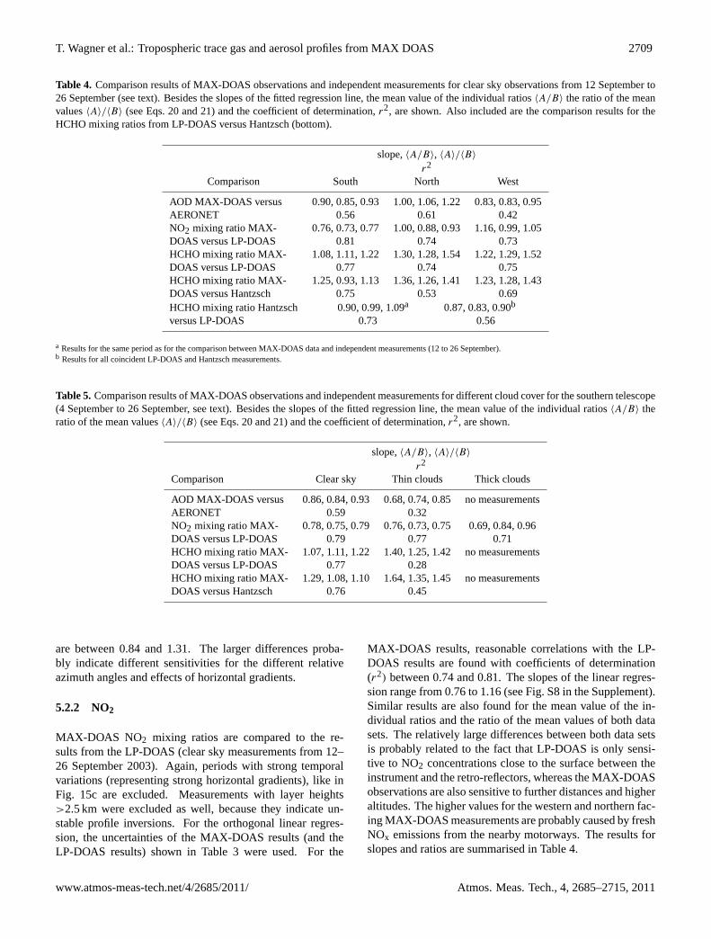
T. Wagner et al.: Tropospheric trace gas and aerosol profiles from MAX DOAS 2709
Table 4. Comparison results of MAX-DOAS observations and independent measurements for clear sky observations from 12 September to26 September (see text). Besides the slopes of the fitted regression line, the mean value of the individual ratios〈A/B〉 the ratio of the meanvalues〈A〉/〈B〉 (see Eqs. 20 and 21) and the coefficient of determination,r2, are shown. Also included are the comparison results for theHCHO mixing ratios from LP-DOAS versus Hantzsch (bottom).
slope,〈A/B〉, 〈A〉/〈B〉
r2
Comparison South North West
AOD MAX-DOAS versus 0.90, 0.85, 0.93 1.00, 1.06, 1.22 0.83, 0.83, 0.95AERONET 0.56 0.61 0.42NO2 mixing ratio MAX- 0.76, 0.73, 0.77 1.00, 0.88, 0.93 1.16, 0.99, 1.05DOAS versus LP-DOAS 0.81 0.74 0.73HCHO mixing ratio MAX- 1.08, 1.11, 1.22 1.30, 1.28, 1.54 1.22, 1.29, 1.52DOAS versus LP-DOAS 0.77 0.74 0.75HCHO mixing ratio MAX- 1.25, 0.93, 1.13 1.36, 1.26, 1.41 1.23, 1.28, 1.43DOAS versus Hantzsch 0.75 0.53 0.69HCHO mixing ratio Hantzsch 0.90, 0.99, 1.09a 0.87, 0.83, 0.90b
versus LP-DOAS 0.73 0.56
a Results for the same period as for the comparison between MAX-DOAS data and independent measurements (12 to 26 September).b Results for all coincident LP-DOAS and Hantzsch measurements.
Table 5. Comparison results of MAX-DOAS observations and independent measurements for different cloud cover for the southern telescope(4 September to 26 September, see text). Besides the slopes of the fitted regression line, the mean value of the individual ratios〈A/B〉 theratio of the mean values〈A〉/〈B〉 (see Eqs. 20 and 21) and the coefficient of determination,r2, are shown.
slope,〈A/B〉, 〈A〉/〈B〉
r2
Comparison Clear sky Thin clouds Thick clouds
AOD MAX-DOAS versus 0.86, 0.84, 0.93 0.68, 0.74, 0.85 no measurementsAERONET 0.59 0.32NO2 mixing ratio MAX- 0.78, 0.75, 0.79 0.76, 0.73, 0.75 0.69, 0.84, 0.96DOAS versus LP-DOAS 0.79 0.77 0.71HCHO mixing ratio MAX- 1.07, 1.11, 1.22 1.40, 1.25, 1.42 no measurementsDOAS versus LP-DOAS 0.77 0.28HCHO mixing ratio MAX- 1.29, 1.08, 1.10 1.64, 1.35, 1.45 no measurementsDOAS versus Hantzsch 0.76 0.45
are between 0.84 and 1.31. The larger differences proba-bly indicate different sensitivities for the different relativeazimuth angles and effects of horizontal gradients.
5.2.2 NO2
MAX-DOAS NO2 mixing ratios are compared to the re-sults from the LP-DOAS (clear sky measurements from 12–26 September 2003). Again, periods with strong temporalvariations (representing strong horizontal gradients), like inFig. 15c are excluded. Measurements with layer heights>2.5 km were excluded as well, because they indicate un-stable profile inversions. For the orthogonal linear regres-sion, the uncertainties of the MAX-DOAS results (and theLP-DOAS results) shown in Table 3 were used. For the
MAX-DOAS results, reasonable correlations with the LP-DOAS results are found with coefficients of determination(r2) between 0.74 and 0.81. The slopes of the linear regres-sion range from 0.76 to 1.16 (see Fig. S8 in the Supplement).Similar results are also found for the mean value of the in-dividual ratios and the ratio of the mean values of both datasets. The relatively large differences between both data setsis probably related to the fact that LP-DOAS is only sensi-tive to NO2 concentrations close to the surface between theinstrument and the retro-reflectors, whereas the MAX-DOASobservations are also sensitive to further distances and higheraltitudes. The higher values for the western and northern fac-ing MAX-DOAS measurements are probably caused by freshNOx emissions from the nearby motorways. The results forslopes and ratios are summarised in Table 4.
www.atmos-meas-tech.net/4/2685/2011/ Atmos. Meas. Tech., 4, 2685–2715, 2011

2710 T. Wagner et al.: Tropospheric trace gas and aerosol profiles from MAX DOAS
NO2 mixing ratios from MAX-DOAS are also comparedfor different cloud cover (clear sky, thin clouds, and thickclouds). For the observations under thin and thick clouds,rather good correlations and similar slopes as exhibited forclear sky conditions are found (see Fig. S9 in the Supple-ment). Obviously the retrieval of NO2 mixing ratios is lessaffected by the presence of clouds compared to the AOD (seeSect. 4.3). The results for slopes and ratios are summarisedin Table 5.
Correlation analyses between the results for the differenttelescopes were also performed (for more details see Fig. S10in the Supplement). During the first part of the campaign,when the telescopes were directed at the same azimuth an-gle (south), good consistency was found: the slopes and ra-tios for the NO2 VCD are between 0.97 and 1.09; the slopesand ratios for the NO2 mixing ratios are between 0.96 and1.04; the slopes and ratios for the NO2 layer height are be-tween 0.97 and 1.06. During the second part of the campaign,when the telescopes were directed at different azimuth angles(north, west, south), as expected less consistency was found:the slopes and ratios for the NO2 VCD are between 0.94 and1.19; the slopes and ratios for the NO2 mixing ratios are be-tween 0.82 and 1.42; the slopes and ratios for the NO2 layerheight are between 0.87 and 1.26. Again, this probably indi-cates different sensitivities for the different relative azimuthangles and effects of horizontal gradients.
5.2.3 HCHO
MAX-DOAS HCHO mixing ratios are compared to resultsfrom the LP-DOAS and the Hantzsch instruments (clear skymeasurements from 12–26 September 2003). Again, periodswith strong temporal variations (representing strong horizon-tal gradients) like in Fig. 15c are excluded. Also measure-ments with layer heights>2.5 km were excluded, becausethey indicate unstable profile inversions. For the orthogo-nal linear regression, the uncertainties of the MAX-DOASresults as shown in Table 3 were used.
For the three telescopes reasonable correlations with re-spect to the results of the LP-DOAS and the Hantzsch in-struments are found; with coefficients of determination (r2)
between 0.53 and 0.77. The slopes of the linear regressionare between 1.08 and 1.36 (see Fig. S11 in the Supplement).Similar results are found for the mean value of the individualratios and the ratio of the mean values of both data sets. Theresults for slopes and ratios are summarised in Table 4.
HCHO mixing ratios from MAX-DOAS are compared fordifferent cloud cover (clear sky and thin clouds). Like forNO2, a rather good correlation with the independent mea-surements is still obtained for thin clouds, but the slope ofthe regression line is now systematically larger than for clearsky conditions (see Fig. S12 in the Supplement). Again, thisfinding can in principle be explained by the diffusing screeneffect on the trace gases profile retrievals (see Sect. 4.3). Theoverestimation is probably caused by the fact that the HCHO
layer extends to higher altitudes than the NO2 layer. The re-sults for slopes and ratios are summarised in Table 5.
It is interesting to note that the correlation between theHantzsch instrument and the LP-DOAS is similar to theMAX-DOAS comparisons with either independent measure-ment, but the slopes and ratios are closer to unity. For thewhole measurement campaign a coefficient of determination(r2) of 0.56 and slope of 0.87 (Hantzsch versus LP-DOAS) isobtained; the mean value of the individual ratios is 0.83 andthe ratio of the mean values is 0.90. If only clear sky obser-vations between 12 and 26 September 2003 are considered,a coefficient of determination (r2) of 0.73 and slope of 0.90(Hantzsch versus LP-DOAS) is obtained; the mean value ofthe individual ratios is 0.99 and the ratio of the mean values is1.09. The results for slopes and ratios are summarised in Ta-ble 4. Similar results have been reported in Hak et al. (2005).However, it should be noted that therein a white cell (notlong path) DOAS instrument was compared to Hantzsch in-struments.
Correlation analyses between the results for the differenttelescopes were performed (for more details see Fig. S13in the Supplement). During the first part of the campaign,when the telescopes were directed at the same azimuth an-gle (south), fair consistency was found: the slopes and ratiosfor the HCHO VCD are between 0.88 and 1.25; the slopesand ratios for the HCHO mixing ratios are between 0.87 and1.11; the slopes and ratios for the HCHO layer height are be-tween 0.83 and 1.31. During the second part of the campaign,when the telescopes were directed at different azimuth an-gles (north, west, south), the consistency was slightly worse:the slopes and ratios for the HCHO VCD are between 0.84and 1.35; the slopes and ratios for the HCHO mixing ratiosare between 0.92 and 1.17; and the slopes and ratios for theHCHO layer height are between 0.81 and 1.43. For HCHO,the uncertainties of the inversion results are generally higher;thus effects of the different sensitivities for the different rel-ative azimuth angles and effects of horizontal gradients arenot as important (compared to other uncertainties) as for theother retrievals.
5.2.4 Trace gas VCDs
So called geometric VCDs (Eq. 17) are often used for thevalidation of satellite observations of tropospheric trace gasVCDs (Brinksma et al., 2008). Since in their determinationscattering by molecules and aerosols is neglected, they areaffected by systematic errors depending on the layer height,AOD and viewing geometry. To estimate these errors, wecompared the “geometric” VCDs (using elevation angles of18◦ and 90◦, see Eq. 17) for NO2 and HCHO to the cor-responding VCDs obtained from the profile inversion (seeFig. S14 in the Supplement). For NO2, relatively good agree-ment is found (slopes and ratios between 0.88 and 1.03),but for HCHO the geometric VCDs systematically underes-timate the VCDs obtained by the profile inversion (slopes
Atmos. Meas. Tech., 4, 2685–2715, 2011 www.atmos-meas-tech.net/4/2685/2011/

T. Wagner et al.: Tropospheric trace gas and aerosol profiles from MAX DOAS 2711
Table 6. Comparison results of geometric trace gas VCDs (using 18◦ and 90◦ elevation angles) versus VCDs from the MAX-DOAS profileretrieval for clear sky observations from 12 to 26 September, see text). Besides the slopes of the fitted regression line, the mean value of theindividual ratios〈A/B〉 the ratio of the mean values〈A〉/〈B〉 (see Eqs. 20 and 21) and the coefficient of determination,r2, are shown.
slope,〈A/B〉, 〈A〉/〈B〉
r2
Comparison South North West
NO2 VCDgeoversus VCD 0.88, 0.88, 0.91 0.96, 0.99, 1.03 0.92, 0.91, 0.96from profile retrieval 0.88 0.96 0.86HCHO VCDgeoversus VCD 0.66, 0.77, 0.84 0.74, 0.88, 0.93 0.67, 0.75, 0.78from profile retrieval 0.71 0.81 0.74
and ratios between 0.66 and 0.93). The results for slopesand ratios are summarised in Table 6. We investigated possi-ble reasons for these dependencies by calculating the relativedifferences between both types of VCDs:
1VCDrel =VCD−VCDgeo
VCD(22)
While no clear correlation of1VCDrel with the AOD wasfound (not shown),1VCDrel shows a systematic dependenceon the layer height (for details of the correlation analyses seeFig. S14 in the Supplement). This dependence indicates thatthe neglect of scattering by molecules and aerosols becomesmore important for vertically extended trace gas layers. Forlayer heights below 1000 m, the error of the geometric VCDis typically within 20 %.
5.3 Comparison to vertical profiles
On several days during the FORMAT-II campaign, verticalprofiles of the HCHO mixing ratio and aerosol particle con-centration were measured from an ultra light aircraft (Junker-mann, 2009). Although due to airspace regulations, thesemeasurements were restricted to areas outside the city of Mi-lano (typical distance to the measurement site was 20 km), itis interesting to compare the obtained profiles with the MAX-DOAS results. Also, the horizontal heterogeneity can be es-timated from the aircraft measurements. Here it is interestingto note that the sensitivity of the MAX-DOAS measurementsis typically limited to within a horizontal distance of about5 km.
The flight patterns flown from the airfield of Spessa, southof Milano consisted of a horizontal flight below 500 m pass-ing east of the restricted airspace of Milano Linate airport fol-lowed by a short descent to about 300 m over the runway ofthe Lecco Monte Marenzo. North of this airfield the permit-ted airspace for visual flight rules extends up to 3000 m a.s.l.The aircraft here flew spirals climbing up to 3000 m over thecity of Lecco and the nearby Lago di Pusiano. A short hor-izontal transect led west to the city of Como, where the de-scent was flown with spirals of a diameter of<3 km. Reach-ing the level of∼500 m a.g.l. the return flight passed Milano
horizontally in the west. South of the river Po a second pro-file was added up to∼1600 m a.s.l. before the flights finallyended at Spessa. Note that on 18 September, a modified flighttrack was chosen with the north-south transect also flown eastof Milano.
In Fig. 17 the HCHO and aerosol profiles are comparedto the MAX-DOAS results for the time of the aircraft mea-surements (±30 min). Note that the aerosol measurementsdo not provide aerosol optical properties, but aerosol con-centration profiles (here profiles of the number densities withradii >300 nm are shown); thus only a qualitative compari-son with the aerosol optical properties retrieved from MAX-DOAS is possible.
The vertical profiles of the aerosol and HCHO in-situ mea-surements were quite different on 18/19 September and 22and 25 September. While the first two days resembled thevertical distributions of clear days without clouds, the lat-ter days were more typical for cloudy conditions with somecloud processing and transport of aerosols and HCHO intolayer above the planetary boundary layer. On the afternoonof 22 September and whole of 25 September clouds werepresent (see Fig. S15).
On 18 and 19 September 2003, similar HCHO and aerosolprofiles were measured from the aircraft (Fig. 17a, b). Theheights of the HCHO and aerosol layers range from 1000 mup to about 1400 m. The vertical gradient of the aerosolconcentration is slightly steeper than that of HCHO. TheHCHO layer height derived from MAX-DOAS is variable,but agrees roughly with the aircraft measurements. In con-trast, the aerosol layer from MAX-DOAS height is systemat-ically lower (by about 100 to 400 m). Besides possible mea-surement and retrieval errors, these differences might also berelated to strong horizontal gradients as indicated by the dif-ference of the profiles south and north of Milano. It shouldbe noted that compared to other parts of the day the MAX-DOAS aerosol layer heights were lower during the aircraftmeasurements.
On 22 September 2003 no clearly defined single layers aremeasured by the aircraft. The HCHO mixing ratios graduallydecrease with altitude. For the aerosol concentration two dis-tinct layers were present. The HCHO layer heights retrieved
www.atmos-meas-tech.net/4/2685/2011/ Atmos. Meas. Tech., 4, 2685–2715, 2011

2712 T. Wagner et al.: Tropospheric trace gas and aerosol profiles from MAX DOAS
9.0 9.2 9.4Longitude [°]
45.0
45.8
Latit
ude
[ ]
Bresso
0 400 800[cm-3]
010
0020
0030
00Al
titud
e [m
]
aircraft
0 4 8[ppt]
010
0020
0030
00Al
titud
e [m
]
aircraftparticles>300nm
N W S N W SMAX-DOAS
N W S
MAX-DOAS
N W S
HCHO Aerosols 18 Sep 2003
9.0 9.2 9.4Longitude [°]
45.0
45.8
Latit
ude
[ ]
Bresso
0 400 800[cm-3]
010
0020
0030
00Al
titud
e [m
]
aircraft
0 4 8[ppt]
010
0020
0030
00Al
titud
e [m
]
aircraftparticles>300nm
N W S N W SMAX-DOAS
N W S
MAX-DOAS
N W S
HCHO Aerosols 18 Sep 2003
9.0 9.2 9.4Longitude [°]
45.0
45.8
Latit
ude
[ ]
Bresso
0 400 800[cm-3]
010
0020
0030
00Al
titud
e [m
]
aircraft
0 4 8[ppt]
010
0020
0030
00Al
titud
e [m
]
aircraftparticles>300nm
N W S N W SMAX-DOAS
N W S
MAX-DOAS
N W S
HCHO Aerosols 19 Sep 2003
9.0 9.2 9.4Longitude [°]
45.0
45.8
Latit
ude
[ ]
Bresso
0 400 800[cm-3]
010
0020
0030
00Al
titud
e [m
]
aircraft
0 4 8[ppt]
010
0020
0030
00Al
titud
e [m
]
aircraftparticles>300nm
N W S N W SMAX-DOAS
N W S
MAX-DOAS
N W S
HCHO Aerosols 19 Sep 2003
9.0 9.2 9.4Longitude [°]
45.0
45.8
Latit
ude
[ ]
Bresso
0 400 800[cm-3]
010
0020
0030
00Al
titud
e [m
]
aircraft
0 4 8[ppt]
010
0020
0030
00Al
titud
e [m
]
particles>300nm
aircraft N W S N W SMAX-DOAS
N W S
MAX-DOAS
N W S
HCHO Aerosols 22 Sep 2003
9.0 9.2 9.4Longitude [°]
45.0
45.8
Latit
ude
[ ]
Bresso
0 400 800[cm-3]
010
0020
0030
00Al
titud
e [m
]
aircraft
0 4 8[ppt]
010
0020
0030
00Al
titud
e [m
]
particles>300nm
aircraft N W S N W SMAX-DOAS
N W S
MAX-DOAS
N W S
HCHO Aerosols 22 Sep 2003
9.0 9.2 9.4Longitude [°]
45.0
45.8
Latit
ude
[ ]
Bresso
0 400 800[cm-3]
010
0020
0030
00Al
titud
e [m
]
aircraft
0 4 8[ppt]
010
0020
0030
00Al
titud
e [m
]
aircraftparticles>300nm
N W SMAX-DOASN W SN W SN W S
HCHO Aerosols 25 Sep 2003
MAX-DOAS
9.0 9.2 9.4Longitude [°]
45.0
45.8
Latit
ude
[ ]
Bresso
0 400 800[cm-3]
010
0020
0030
00Al
titud
e [m
]
aircraft
0 4 8[ppt]
010
0020
0030
00Al
titud
e [m
]
aircraftparticles>300nm
N W SMAX-DOASN W SN W SN W S
HCHO Aerosols 25 Sep 2003
MAX-DOAS
Fig. 17 Vertical profiles of the aerosol number density (for radii > 300nm) and HCHO mixing ratio measured by an ultra light aircraft. The respective flight tracks and the location of Bresso are indicated in the right part of the figure. Also shown are the layer heights retrieved from MAX-DOAS at Bresso during the period (±30 min) of the aircraft measurements.
54
Fig. 17. Vertical profiles of the aerosol number density (for radii>300 nm) and HCHO mixing ratio measured by an ultra light aircraft. Therespective flight tracks and the location of Bresso are indicated in the right part of the figure. Also shown are the layer heights retrieved fromMAX-DOAS at Bresso during the period (±30 min) of the aircraft measurements.
from MAX-DOAS are between 900 and 1300 m. The aerosollayer heights retrieved from MAX-DOAS are slightly higherthan the lowest aerosol layer. Again large horizontal gradi-ents of the aerosol concentration were measured by the air-craft.
On 25 September 2003 rather high layer heights (up toabout 2000 m) were measured from the aircraft. Higher layerheights are also retrieved from MAX-DOAS; in particular theaerosol layer height agrees well with the aircraft profiles.
It is interesting to note that the HCHO mixing ratios werenot correlated to large particles but were nearly proportionalthe small (ultra-fine) particle concentrations. These parti-cles are co-emitted with HCHO during the frequent biomassburning events. This result is possibly not relevant for theHCHO MAX-DOAS measurements but explains the compa-rably high mixing ratios in the south.
Atmos. Meas. Tech., 4, 2685–2715, 2011 www.atmos-meas-tech.net/4/2685/2011/

T. Wagner et al.: Tropospheric trace gas and aerosol profiles from MAX DOAS 2713
6 Summary and conclusions
In this study a simple profile inversion scheme for the re-trieval of aerosol extinction and trace gas concentrationsfrom MAX-DOAS observations (similar to that developed byLi et al., 2010) is applied to MAX-DOAS measurements dur-ing the FORMAT-II campaign in September 2003 in Bresso(north of Milano, Italy) from 4–26 September 2003. Asimilar prototype study for MAX-DOAS profile retrievalsfor a limited data set was already conducted by Heckel etal. (2005). Our inversion scheme yields two profile param-eters: besides the integrated quantities (trace gas VCD oraerosol optical depth), the layer height is also determined;from both quantities the average aerosol extinction or tracegas concentration is also obtained. In principle, informationon the relative profile shape could be derived, but for ourmeasurements only two independent parameters could be re-trieved in a standardised way for all measurements. The pro-file inversion is performed for individual elevation sequenceswith a time resolution for individual profiles of about 10 min.Profile inversions were possible on 23 days (with severalgaps mainly caused by clouds). According to the retrievedtrace gas and aerosol data, three characteristic periods can bedistinguished: The first period (4–14 September 2003) waspartly cloudy with relatively low AOD and trace gas mix-ing ratios. The second period (from 15–22 September 2003)was characterised by many clear days (see also Junkermann,2009; Liu et al., 2007; Steinbacher et al., 2005a, b; Wit-trock, 2006) with enhanced with enhanced AODs and tracegas mixing ratios.
The third period (23–26 September 2003) was similar tothe first period. For HCHO and aerosols in general similarlayer heights were found; the NO2 layer height was typicallylower than for HCHO and aerosols, but increased systemat-ically during the day. The temporal evolution of the MAX-DOAS results is similar to those described in other studiesof the FORMAT-II campaign (Junkermann, 2009; Liu et al.,2007; Steinbacher et al., 2005a, b; Wittrock, 2006).
One speciality of our MAX-DOAS observations is thesimultaneous measurement from three separate telescopes.During the first part of the campaign, the three telescopeswere directed to the same azimuth angle (towards the south).From the differences between the results for the three tele-scopes the inherent precision of the profile inversions can beestimated. We estimated the consistency between the dif-ferent telescopes from the slopes of the correlation analysisand the ratios between the respective results (see Sect. 5.2).For the aerosol profile inversion, the optical depths and layerheights for the three telescopes were consistent within±10 %and±7 %, respectively. For the NO2 profile inversion, theVCDs, mixing ratios and layer heights were consistent within±9 %,±4 %, and±6 %, respectively. For the HCHO profileinversion the VCDs, mixing ratios and layer heights wereconsistent within±25 %, ±13 %, and±31 %, respectively.The larger deviations of the HCHO results probably mainly
reflect the larger errors of the DOAS retrieval, because the at-mospheric HCHO absorptions are typically weaker than theNO2 absorption.
During the second part of the campaign, the three tele-scopes were directed at three different azimuth angles (north,west, south). Now, larger differences between the three tele-scopes are found, which also reflect the effects of differentrelative azimuth angles and the spatio-temporal variabilityof the aerosol and trace gas concentrations. For the aerosolprofile inversion, the optical depths and layer heights for thethree telescopes were consistent within±38 % and±36 %,respectively. For the NO2 profile inversion the VCDs, mix-ing ratios and layer heights were consistent within±19 %,±42 %, and±26 %, respectively. For the HCHO profile in-version the VCDs, mixing ratios, and layer heights were con-sistent within±35 %,±24 %, and±43 %, respectively. Thelarge differences for the NO2 mixing ratios are probably re-lated to large horizontal gradients at the measurement sitecaused by nearby motorways in northerly and westerly di-rections. Here it might be interesting to note that possiblefuture inversions algorithms for MAX-DOAS measurementswith different azimuth angles might retrieve not only verticalprofiles, but also horizontal gradients in one inversion step.
In addition to the comparisons between the different tele-scopes, the MAX-DOAS results were compared to the re-sults of independent measurements. Depending on the view-ing direction, the AODs retrieved from the MAX-DOAS ob-servations were either found to be smaller or larger than theAERONET AODs (slopes of the regression lines and ratiosbetween the data sets between 0.83 and 1.22). Here it shouldbe noted that the AERONET station at Ispra is located about50 km north-west of Bresso.
The NO2 mixing ratios retrieved from MAX-DOAS areeither smaller or larger than the results from the long pathDOAS (slopes of the regression lines and average ratios be-tween the data sets between 0.73 and 1.16). The HCHO mix-ing ratios retrieved from the MAX-DOAS observations aremostly higher than those retrieved from the long path DOAS(slopes of the regression lines and average ratios between thedata sets between 1.08 and 1.54), and the Hantzsch instru-ment (slopes of the regression lines and average ratios be-tween the data sets between 1.23 and 1.43). The correlationbetween the MAX-DOAS results and the independent mea-surements is similar to the correlation between both indepen-dent measurements themselves (Hantzsch instrument versuslong path DOAS).
On 4 days, vertical profiles of HCHO and aerosols mea-sured from an ultra light aircraft were available and werecompared to the respective MAX-DOAS layer heights. Theaircraft was flown around Milano, but unfortunately mea-surements directly above Bresso were not available due toairspace restrictions. Overall, reasonable agreement with theMAX-DOAS profile heights was found. Deviations might in-dicate errors of the MAX-DOAS measurements or the profileretrieval, but are probably also related to horizontal gradients.
www.atmos-meas-tech.net/4/2685/2011/ Atmos. Meas. Tech., 4, 2685–2715, 2011

2714 T. Wagner et al.: Tropospheric trace gas and aerosol profiles from MAX DOAS
Besides the profile inversions for aerosols and trace gases,an important aspect of our study was to investigate the ef-fects of clouds on the inversion results. For that purpose,a cloud discrimination scheme was developed and applied,which makes use of the results of the zenith viewing di-rections of the MAX-DOAS measurements. Based on thisscheme, the effects of clouds on the profile inversion resultswere investigated. It was found that the aerosol optical depthis systematically underestimated and the HCHO mixing ra-tio is systematically overestimated in the presence of clouds.In contrast, the NO2 mixing ratios are only slightly affected.These findings could be in principle reproduced by radiativetransfer simulations.
Our study demonstrates that a simple profile inversion pro-cedure for aerosols and trace gases can be successfully ap-plied to MAX-DOAS observations in the UV. Together withthe cloud classification scheme this method is well suitedfor use on a routine basis. One important limitation of ourMAX-DOAS observations was the lack of very low eleva-tion angles (<3◦). Future measurements should include suchlow elevation angles to improve the sensitivity of the methodto retrieve relative profile shapes.
Supplementary material related to thisarticle is available online at:http://www.atmos-meas-tech.net/4/2685/2011/amt-4-2685-2011-supplement.zip.
Acknowledgements.The authors would like to thank the staff of theItalian Red Cross section at the airport in Bresso (Milano), wherethe measurements were carried out, for their great hospitality.Financial support from the EU is highly appreciated (project FOR-MAT, http://www.nilu.no/format/, grant EVK2-CT-2001-00120).Aerosol data from the AERONET station at Ispra (Italy) were usedfor comparison with our results. Many thanks to the PrincipalInvestigator, Giuseppe Zibordi, for his effort in establishing andmaintaining the AERONET station at Ispra. MODIS imageswere obtained from NASA/GSFC, MODIS Rapid Response,http://aeronet.gsfc.nasa.gov/cgi-bin/bamgomasinteractive.
The service charges for this open access publicationhave been covered by the Max Planck Society.
Edited by: K. Strong
References
Brinksma, E. J., Pinardi, G., Braak, R., Volten, H., Richter, A.,Schonhardt, A., van Roozendael, M., Fayt, C., Hermans, C.,Dirksen, R. J., Vlemmix, T., Berkhout, A. J. C., Swart, D. P.J.,Otjen, H., Wittrock, F., Wagner, T., Ibrahim, O. W., de Leeuw,G., Moerman, M., Curier, R. L., Celarier, E. A., Knap, W. H.,Veefkind, J. P., Eskes, H. J., Allaart, M., Rothe, R., Piters, A.J. M., and Levelt, P. F.: The 2005 and 2006 DANDELIONSNO2 and Aerosol Validation Campaigns, J. Geophys. Res., 113,D16S46,doi:10.1029/2007JD008808, 2008.
Cantrell, C. A.: Technical Note: Review of methods for linear least-squares fitting of data and application to atmospheric chemistryproblems, Atmos. Chem. Phys., 8, 5477–5487,doi:10.5194/acp-8-5477-2008, 2008.
Clemer, K., Van Roozendael, M., Fayt, C., Hendrick, F., Hermans,C., Pinardi, G., Spurr, R., Wang, P., and De Maziere, M.: Mul-tiple wavelength retrieval of tropospheric aerosol optical proper-ties from MAXDOAS measurements in Beijing, Atmos. Meas.Tech., 3, 863–878,doi:10.5194/amt-3-863-2010, 2010.
Deutschmann, T.: Atmospheric Radiative Transfer Modelling withMonte Carlo Methods, Diploma thesis, University of Heidelberg,2008.
Deutschmann, T., Beirle, S., Frieß, U., Grzegorski, M., Kern, C.,Kritten, L., Platt, U., Pukite, J., Wagner, T., Werner, B., andPfeilsticker, K.: The Monte Carlo Atmospheric Radiative Trans-fer Model McArtim: Introduction and Validation of Jacobiansand 3D Features, J. Quant. Spectrosc. Ra., 112, 1119–1137,doi:10.1016/j.jqsrt.2010.12.009, 2011.
Dubovik, O., Holben, B. N., Eck, T. F., Smirnov, A., Kaufman, Y.J., King, M. D., Tanre, D., and Slutsker, I.: Variability of ab-sorption and optical properties of key aerosol types observed inworldwide locations, J. Atmos. Sci., 59, 590–608, 2002.
Erle, F., Pfeilsticker, K., and Platt, U.: On the influence of tropo-spheric clouds on zenith-scattered-light measurements of strato-spheric species, Geophys. Res. Lett., 22, 2725–2728, 1995.
Frieß, U., Monks, P. S., Remedios, J. J., Rozanov, A., Sinre-ich, R., Wagner, T., and Platt, U.: MAX-DOAS O4 measure-ments: A new technique to derive information on atmosphericaerosols. (II) Modelling studies, J. Geophys. Res., 111, D14203,doi:10.1029/2005JD006618, 2006.
Greenblatt, G. D., Orlando, J. J., Burkholder, J. B., and Ravis-hankara, A. R.: Absorption measurements of oxygen between330 and 1140 nm, J. Geophys. Res., 95, 18577–18582, 1990.
Hak, C.: Variability of formaldehyde in the polluted planetaryboundary layer – measurements in the Milano metropolitan area,Italy (Po basin), PhD-thesis, University of Karlsruhe, 2006.
Hak, C., Pundt, I., Trick, S., Kern, C., Platt, U., Dommen, J.,Ordonez, C., Prevot, A. S. H., Junkermann, W., Astorga-Llorens,C., Larsen, B. R., Mellqvist, J., Strandberg, A., Yu, Y., Galle, B.,Kleffmann, J., Lorzer, J. C., Braathen, G. O., and Volkamer, R.:Intercomparison of four different in-situ techniques for ambientformaldehyde measurements in urban air, Atmos. Chem. Phys.,5, 2881–2900,doi:10.5194/acp-5-2881-2005, 2005.
Heckel, A., Richter, A., Tarsu, T., Wittrock, F., Hak, C., Pundt, I.,Junkermann, W., and Burrows, J. P.: MAX-DOAS measurementsof formaldehyde in the Po-Valley, Atmos. Chem. Phys., 5, 909–918,doi:10.5194/acp-5-909-2005, 2005.
Holben, B. N., Tanre, D., Smirnov, A., Eck, T. F., Slutsker, I.,Abuhassan, N., Newcomb, W. W., Schafer, J., Chatenet, B., Lav-enue, F., Kaufman, Y. J., Vande Castle, J., Setzer, A., Markham,B., Clark, D., Frouin, R., Halthore, R., Karnieli, A., O’Neill, N.T., Pietras, C., Pinker, R. T., Voss, K., and Zibordi, G.: An emerg-ing ground-based aerosol climatology: Aerosol Optical Depthfrom AERONET, J. Geophys. Res., 106, 12 067–12 097, 2001.
Honninger, G. and Platt, U.: Observations of BrO and its verticaldistribution during surface ozone depletion at Alert, Atmos. En-viron., 36, 2481–2490, 2002.
Irie, H., Kanaya, Y., Akimoto, H., Iwabuchi, H., Shimizu, A., andAoki, K.: First retrieval of tropospheric aerosol profiles using
Atmos. Meas. Tech., 4, 2685–2715, 2011 www.atmos-meas-tech.net/4/2685/2011/
T. Wagner et al.: Tropospheric trace gas and aerosol profiles from MAX DOAS 2715
MAX-DOAS and comparison with lidar and sky radiometer mea-surements, Atmos. Chem. Phys., 8, 341–350,doi:10.5194/acp-8-341-2008, 2008.
Irie, H., Kanaya, Y., Akimoto, H., Iwabuchi, H., Shimizu, A.,and Aoki, K.: Dual-wavelength aerosol vertical profile measure-ments by MAX-DOAS at Tsukuba, Japan, Atmos. Chem. Phys.,9, 2741–2749,doi:10.5194/acp-9-2741-2009, 2009.
Junkermann, W.: On the distribution of formaldehyde in the west-ern Po-Valley, Italy, during FORMAT 2002/2003, Atmos. Chem.Phys., 9, 9187–9196,doi:10.5194/acp-9-9187-2009, 2009.
Junkermann, W. and Burger, J. M.: A new portable instrument forcontinuous measurement of formaldehyde in ambient air, J. At-mos. Ocean. Tech., 23, 38–45, 2006.
Kelly, T. J. and Fortune, C. R.: Continuous monitoring of gaseousformaldehyde using an improved fluorescence approach., Int. J.Environ. An. Ch., 54, 249–263, 1994.
Li, X., Brauers, T., Shao, M., Garland, R. M., Wagner, T.,Deutschmann, T., and Wahner, A.: MAX-DOAS measurementsin southern China: retrieval of aerosol extinctions and validationusing ground-based in-situ data, Atmos. Chem. Phys., 10, 2079–2089,doi:10.5194/acp-10-2079-2010, 2010.
Liu, L., Andreani-Aksoyoglu, S., Keller, J., Ordonez, C., Junker-mann, W., Hak, C., Braathen, G. O., Reimann, S., Astorga-Llorens, C., Schultz, M., Prevot, A. S. H., and Isaksen, I. S.A.: A photochemical modeling study of ozone and formalde-hyde generation and budget in the Po basin, J. Geophys. Res.,112, D22303,doi:10.1029/2006JD008172, 2007.
Matsui, H., Koike, M., Kondo, Y., Takegawa, N., Fast, J. D.,Poschl, U., Garland, R. M., Andreae, M. O., Wiedensohler, A.,Sugimoto, N., and Zhu, T.: Spatial and temporal variations ofaerosols around Beijing in summer 2006: 2. Local and col-umn aerosol optical properties, J. Geophys. Res.-Atmos., 115,D22207,doi:10.1029/2010JD013895, 2010.
Meller, R. and Moortgat, G. K.: Temperature dependence of the ab-sorption cross sections of formaldehyde between 223 and 323 Kin the wavelength range 225–375 nm, J. Geophys. Res., 105,7089–7101, 2000.
Platt, U. and Stutz, J.: Differential Optical Absorption Spec-troscopy, Principles and Applications, Springer, Berlin, 2008.
Pundt, I. and Mettendorf, K. U.: The Multibeam long path differen-tial optical absorption spectroscopy instrument: A device for si-multaneous measurements along multiple light paths, Appl. Op-tics, 44, 4985–4994, 2005.
Rodgers, C. D.: Inverse Methods for Atmospheric Sounding: The-ory and Practice, Ser. Atmos. Oceanic Planet. Phys., F. W. Taylor,World Sci., Hackensack, NY, 2, 2000.
Roscoe, H. K., Van Roozendael, M., Fayt, C., du Piesanie, A.,Abuhassan, N., Adams, C., Akrami, M., Cede, A., Chong, J.,Clemer, K., Friess, U., Gil Ojeda, M., Goutail, F., Graves, R.,Griesfeller, A., Grossmann, K., Hemerijckx, G., Hendrick, F.,Herman, J., Hermans, C., Irie, H., Johnston, P. V., Kanaya, Y.,Kreher, K., Leigh, R., Merlaud, A., Mount, G. H., Navarro, M.,Oetjen, H., Pazmino, A., Perez-Camacho, M., Peters, E., Pinardi,G., Puentedura, O., Richter, A., Schonhardt, A., Shaiganfar, R.,Spinei, E., Strong, K., Takashima, H., Vlemmix, T., Vrekoussis,M., Wagner, T., Wittrock, F., Yela, M., Yilmaz, S., Boersma,F., Hains, J., Kroon, M., Piters, A., and Kim, Y. J.: Inter-comparison of slant column measurements of NO2 and O4 byMAX-DOAS and zenith-sky UV and visible spectrometers, At-
mos. Meas. Tech., 3, 1629–1646,doi:10.5194/amt-3-1629-2010,2010.
Sinreich, R., Frieß, U., Wagner, T., and Platt, U.: Multi axisdifferential optical absorption spectroscopy (MAX-DOAS) ofgas and aerosol distributions, Faraday Discuss., 130, 153–164,doi:10.1039/b419274p, 2005.
Solomon, S., Schmeltekopf, A. L., and Sanders, R. W.: On the in-terpretation of zenith sky absorption measurements, J. Geophys.Res., 92, 8311–8319, 1987.
Steinbacher, M., Dommen, J., Ordonez, C., Reimann, S., Grubler,F. C., Staehelin, J., and Prevot, A. S. H.: Volatile organic com-pounds in the Po Basin. Part A: Anthropogenic VOCs, J. Atmos.Chem., 51, 271–291, 2005a.
Steinbacher, M., Dommen, J., Ordonez, C., Reimann, S., Staehe-lin, S., Andreani-Aksoyoglu, S., and Prevot, A. S. H.: Volatileorganic compounds in the Po Basin. Part B: biogenic VOCs, J.Atmos. Chem., 51, 293–315, 2005b.
Van Roozendael, M., Fayt, C., Post, P., Hermans, C., and Lambert,J.-C.: Retrieval of BrO and NO2 from UV-Visible Observations,in: Sounding the troposphere from space: a new era for atmo-spheric chemistry, edited by Borrell, P. M., Burrows, J. P., Platt,U., Springer, Heidelberg, ISBN 3-540-40873-8, 2003.
Voigt, S., Orphal, J., and Burrows, J. P.: The temperature andpressure dependence of the absorption cross-sections of NO2in the 250–800 nm region measured by Fourier-transform spec-troscopy, J. Photoch. Photobio. A, 149, 1–7, 2002.
Wagner, T., Erle, F., Marquard, L., Otten, C., Pfeilsticker, K., Senne,T., Stutz, J., and Platt, U.: Cloudy sky optical paths as derivedfrom differential optical absorption spectroscopy observations,J. Geophys. Res., 103, 25307–25321, 1998.
Wagner, T., Dix, B., v. Friedeburg, C., Frieß, U., Sanghavi, S.,Sinreich, R., and Platt, U.: MAX-DOAS O4 measurements –a new technique to derive information on atmospheric aerosols.(I) Principles and information content, J. Geophys. Res., 109,D22205,doi:10.1029/2004JD004904, 2004.
Wagner, T., Deutschmann, T., and Platt, U.: Determination ofaerosol properties from MAX-DOAS observations of the Ringeffect, Atmos. Meas. Tech., 2, 495–512,doi:10.5194/amt-2-495-2009, 2009.
Winterrath, T., Kurosu, T. P., Richter, A., and Burrows, J. P.: En-hanced O3 and NO2 in thunderstorm clouds: convection or pro-duction?, Geophys. Res. Lett., 26, 1291–1294, 1999.
Wittrock, F.: The retrieval of oxygenated volatile organic com-pounds by remote sensing techniques, PhD thesis, University ofBremen, available at:http://elib.suub.uni-bremen.de/diss/docs/00010481.pdf, 2006.
Wittrock, F., Oetjen, H., Richter, A., Fietkau, S., Medeke, T.,Rozanov, A., and Burrows, J. P.: MAX-DOAS measurementsof atmospheric trace gases in Ny-Alesund – Radiative transferstudies and their application, Atmos. Chem. Phys., 4, 955–966,doi:10.5194/acp-4-955-2004, 2004.
Zieger, P., Weingartner, E., Henzing, J., Moerman, M., de Leeuw,G., Mikkil a, J., Ehn, M., Petaja, T., Clemer, K., van Roozen-dael, M., Yilmaz, S., Frieß, U., Irie, H., Wagner, T., Shaigan-far, R., Beirle, S., Apituley, A., Wilson, K., and Baltensperger,U.: Comparison of ambient aerosol extinction coefficients ob-tained from in-situ, MAX-DOAS and LIDAR measurements atCabauw, Atmos. Chem. Phys., 11, 2603–2624,doi:10.5194/acp-11-2603-2011, 2011.
www.atmos-meas-tech.net/4/2685/2011/ Atmos. Meas. Tech., 4, 2685–2715, 2011