Inverse problems in earth observation and cartography

Shape modelling via higher-order active

contours and phase fields

Ian JermynJosiane Zerubia

Marie RocheryPeter Horvath

Ting PengAymen El Ghoul

2

Overview

Problem: entity extraction from (remote sensing) images. Need for prior ‘shape’ knowledge.

Modelling prior shape knowledge: higher-order active contours (HOACs). Two examples: networks (roads) and circles (tree crowns). Difficulties.

Phase fields: What are they and why use them? Phase field HOACs. Two examples: networks (roads) and circles (tree crowns).

Future.

3

Problem: entity extraction

Ubiquitous in image processing and computer vision: Find in the image the region occupied by particular

entities. E.g. for remote sensing: road network, tree crowns,…

4

Calculate a MAP estimate of the region:

In practice, minimize an energy:

Problem formulation

R = argmaxR

P(RjI ;K )

P(RjI ;K ) / P(I jR;K )P(RjK )

R = argminR

E (R;I )

E (R;I ) = ¡ lnP(I jR;K ) ¡ lnP(RjK )

= E I (I ;R) +EG (R) +const

5

Building EG: active contours

A region is represented by its boundary, R = [], the ‘contour’.

Standard prior energies: Length of R and area of R. Single integrals over the

region boundary: Short range dependencies. Boundary smoothness.

Insufficient prior knowledge.

RR

S1

R2

6

Difficulties

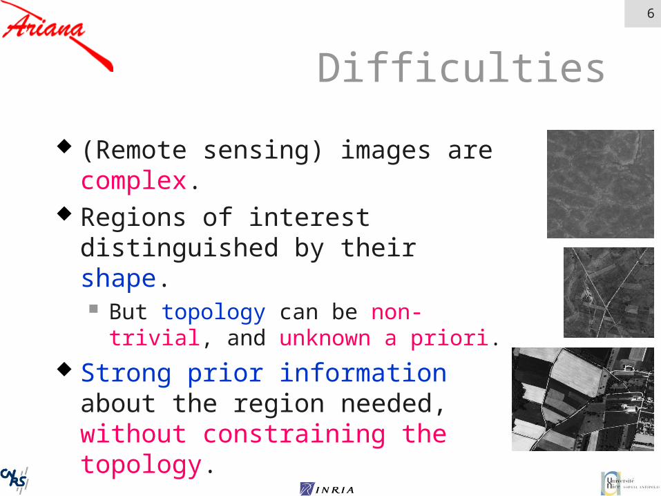
(Remote sensing) images are complex.

Regions of interest distinguished by their shape. But topology can be non-trivial, and

unknown a priori. Strong prior information about the

region needed, without constraining the topology.

7

Building a better EG: higher-order active contours

Introduce prior knowledge via long-range dependencies between tuples of points.

How? Multiple integrals over the contour. E.g. Euclidean invariant two-point term:

Dependent°(t); _°(t)°(t0); _°(t0)

E (°) = ¡ZZ

dt dt0 _°(t) ¢_°(t0) ª (j°(t) ¡ °(t0)j)

8

Prior for networks

Gradient descent with this energy. A perturbed circle evolves towards a structure

composed of arms joining at junctions.

EG (R) =¸L(@R) +®A(R)

¡¯2

ZZdt dt0 _°(t) ¢_°(t0) ª (j°(t) ¡ °(t0)j)

r

r)

9

Prior for a gas of circles

The same energy EG can model a ‘gas of circles’ for certain parameter ranges. Which ranges?

A circle should be a stable configuration of the energy (local minimum). Stability analysis.

10

Phase diagrams

Circle Bar

11

Optimization problem

Minimize E(R, I) = EI(I, R) + EG(R). Algorithm: gradient descent using distance

function level sets. But the gradient of the HOAC term is non-local,

and requires: The extraction of the contour; Many integrations around the contour; Velocity extension.

12

Example I: HOAC results

13

Example I: HOAC results

14

Example II: HOAC results

15

Example II: HOAC results

16

Problems with HOACs

Modelling: Space of regions is complicated to express in the

contour representation. Probabilistic formulation is difficult.

Parameter and model learning are hampered.

Algorithm: Not enough topological freedom. Gradient descent is complex to implement for

higher-order terms. Slow.

Solution: ‘phase fields’.

17

Phase fields

Phase fields are a level set representation (z() = {x : (x) > z}), but the functions, , are unconstrained.

How do we know we are modelling regions?

R

R = 1

R = -1

E0(Á) =Z

­d2x

½D2r Á¢r Á+ ¸(

14Á4 ¡

12Á2)

¾

ÁR = arg minÁ: ³ (Á)=R

E0(R)

18

One can show that

R is a minimum for fixed R. Thus gradient descent with E0 mimics

gradient descent with L: ‘valley following’.

Can also add odd potential term to mimic:

Relation to active contours

R1

R2R3

E0(ÁR ) ' ¸C L(@R)

E0(ÁR ) ' ¸C L(@R) +®CA(R)

19

Why use them?

Complex topologies are easily represented. Representation space is linear:

can be expressed, e.g., in wavelet basis for multiscale analysis of shape.

Probabilistic formulation (relatively) simple. Gradient descent is based solely on the PDE

arising from the energy functional: No reinitialization or ad hoc regularization. Implementation is simple and the algorithm is fast.

20

Why use them?

Neutral initialization: No initial region. No bias towards “interior” or

“exterior”. Greater topological freedom:

Can change number of connected components and number of handles without splitting or wrapping.

+

21

How to write HOACs as phase fields?

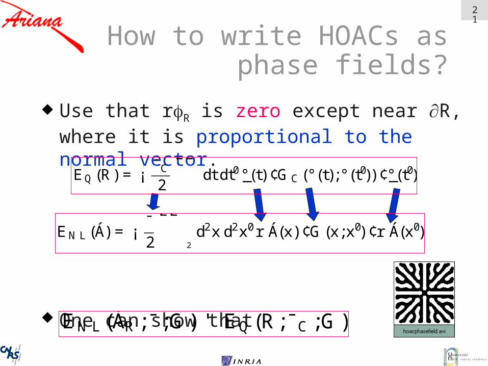
Use that rR is zero except near R, where it is proportional to the normal vector.

One can show that

EQ (R) = ¡¯C2

ZZdt dt0 _°(t) ¢GC (°(t);°(t0)) ¢_°(t0)

EN L (Á) = ¡¯2

ZZ

­ 2d2x d2x0r Á(x) ¢G(x;x0) ¢r Á(x0)

EN L (ÁR ;¯ ;G) ' EQ (R;¯C ;G)

22

Phase fields : likelihood energies EI

r : normal vector to the contour. r¢r : boundary indicator. (1 § )/2 : characteristic function of the region

(+) or its complement (-). Using these elements, one can construct the

equivalents of active contour and HOAC likelihoods.

23

Optimization problem

Minimize

Algorithm: gradient descent, but…

E (R;I ) = E I (I ;R) +EG (R)

= E I (I ;R) +E0(R) +EN L (R)

24

Major advantage of phase fields for HOAC energies

Whereas, due to the multiple integrals, HOAC terms require Contour extraction, contour integrations, and force

extension, Phase field HOACs require only a

convolution:

±EN L±Á(x)

= ¯Z

­d2x0r 2G(x ¡ x0)Á(x0)

25

Phase field HOACs: results

26

Phase field HOACs: VHR image results

27

Phase field HOACs: tree crown results

28

Phase field HOACs: results

29

Future

New prior models Directed and rectilinear networks (rivers, big

cities…). ‘Gas of rectangles’; Controlled perturbed circle.

Multiscale models; New algorithms (multiscale, stochastic,…); Parameter estimation; Higher-dimensions; …

30

Thank you

31

Stability analysis

EC;g(°0+ ±°) =

"

¸C2¼r0+ ®C¼r20 ¡

¯C22¼

Z 2¼

0F00dp

#

+a0

"

¸C2¼+ ®C2¼r0 ¡¯C24¼

Z 2¼

0F10dp

#

+X

kjakj

2"

¸C¼r0k2+ ®C¼

¡¯C24¼

( Ã

2Z 2¼

0F20dp+

Z 2¼

0F21e

ir0kpdp

!

+ k

Ã

2ir0Z 2¼

0F23e

ir0kpdp

!

+k2Ã

r20

Z 2¼

0F24e

ir0kpdp

! ) #

32

HOACs: EI

Linear term that favours large gradients normal to contour.

Quadratic term that favours pairs of points with tangents and image gradients parallel or anti-parallel.

E I ;1(°) =Z

S1dt _°(t) £ r I (°(t))

tangent vectors

gradients

weighting function

E I ;2(°) = ¡ZZ

dt dt0 _° ¢_°0(r I ¢r I 0) ª (j°(t) ¡ °(t0)j)

34

Nonlinearity in the model, not the representation: example

Probability distribution P on R2. P pushes forward to Q on S1. If P is strongly peaked at r0 then

Q() ' P(r0, ). Gradient descent with –ln(P) on R2

mimics gradient descent with -ln(Q) on S1 (‘valley following’).

P (r;µ) = d2x e¡ E (r;µ)

£ exp ¡ ( r4

4 ¡ r22 )

35

Turing stability

To avoid decay of interior and exterior, we require stability of functions § = § 1: 2E/2 must be positive definite (E = E0 + ENL).

For prior terms, this is diagonal in the Fourier basis:

Gives condition on parameters. Better result would be existence and

uniqueness of R for ‘any’ R.

±2E±Á(k0)±Á(k)

(Á§ ) = ±(k;k0)nk2(D ¡ ¯G(k)) +2(¸ ¨ ®)

o