inventory routing - diku.dk · PDF fileInventory Routing Course: Optimization problems in production planning Simon Spoorendonk DIKU, ... Conventional Inventory Management Customer:

Inventory Routing

Course: Optimization problems in production planning

Simon SpoorendonkDIKU, University of Copenhagen

September 21st, 2006

With help from:

Slides of Savelsbergh at VRP Summer School in Montreal 2006.

http://neumann.hec.ca/chairedistributique/en/school2006_en.shtml

1

2

Overview

• Motivation

• Problem Description

• Deterministic [Campbell and Savelsbergh (2004)]

• Stochastic [Kleywegt et al. (2002,2004)]

• Results

Course: Optimization problems in production planning Spoorendonk, DIKU

3

Motivation

Industries with replenishing goods:

• Petrochemical Industry, e.g. oil, gas

• Suppliers for supermarkets

• Department store chains, e.g. Walmart

• Automotive industry, e.g. parts distribution

Combines:

• Inventory Management

• Vehicle Routing


4

Conventional Inventory Management

Customer:

• Monitors inventory levels

• Places orders

Vendor:

• Manufactures/purchases product

• Assembles orders

• Load vehicles

• Routes deliveries

• Makes deliveries

Problems:

• Large variation in demands, production, and transportation

• Workload balancing

• Utilization of resources

• Unnecessary transportation costs

• Urgent vs. nonurgent orders

• Setting priorities


5

Vendor Managed Inventory (VMI)

Customer:

• Trust vendor to manage the inventory

Vendor:

• Monitor customer’s inventory

• Controls inventory replenishment and decides

– When to deliver

– How much to deliver

– How to deliver

VMI transfers inventory (and possible ownership) from customer

to supplier.

VMI synchronizes the supply chain through the process of col-

laborative order fulfillment.


6

Advantages of VMI

Customer:

• Less resources for inventory management

• Assurance that product will be available when required

Vendor:

• More freedom in when and how to manufacture product and

make deliveries

• Better coordination of inventory levels at different customers

• Better coordination of deliveries to decrease transportation

costs.


7

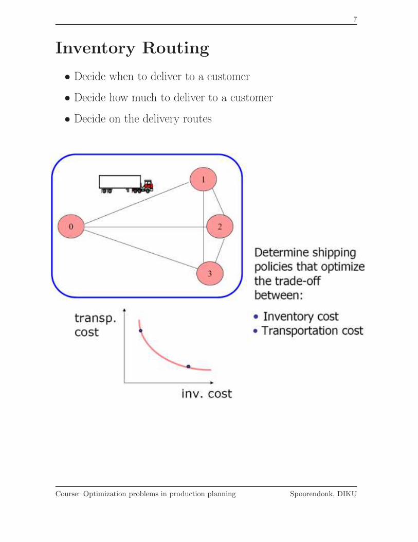
Inventory Routing

• Decide when to deliver to a customer

• Decide how much to deliver to a customer

• Decide on the delivery routes


8

Problem Setting

Single plant:

• Single facility

• Single product

• Set of customers

• Set of homogeneous vehicles

Each customer:

• Storage capacity

• Initial inventory

• Product usage rate or

• Probability distribution of product usage

Shipping policy:

• Zero inventory ordering

• Frequency based periodic shipping

• Deterministic order-up-to level

Objective:

• Minimize distribution costs without causing stock-out on fi-

nite time horizon or

• Maximize the expected total discounted value (rewards mi-

nus cost) over an infinite time horizon


9

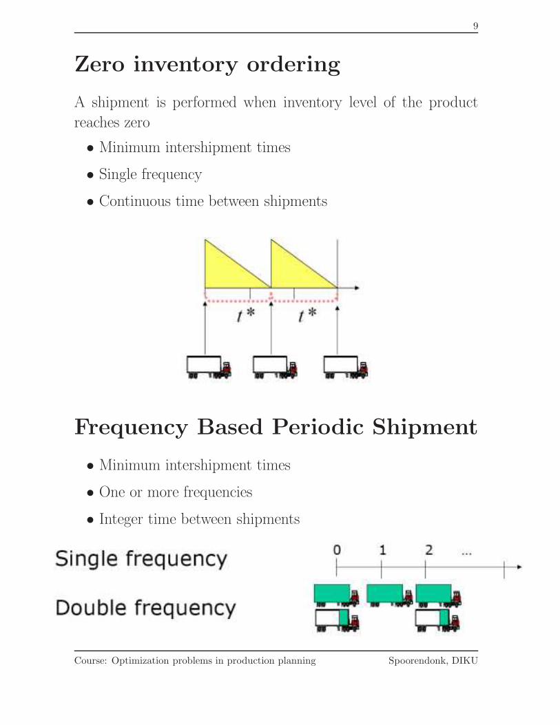
Zero inventory ordering

A shipment is performed when inventory level of the product

reaches zero

• Minimum intershipment times

• Single frequency

• Continuous time between shipments

Frequency Based Periodic Shipment

• Minimum intershipment times

• One or more frequencies

• Integer time between shipments


10

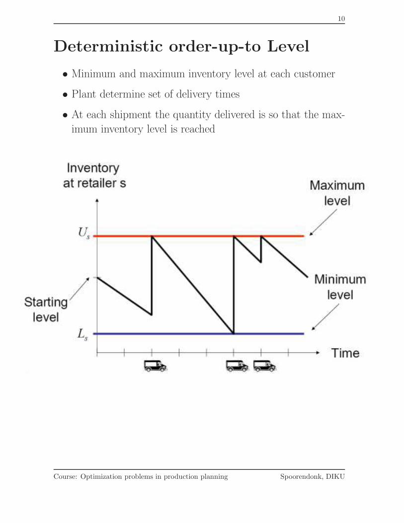
Deterministic order-up-to Level

• Minimum and maximum inventory level at each customer

• Plant determine set of delivery times

• At each shipment the quantity delivered is so that the max-

imum inventory level is reached


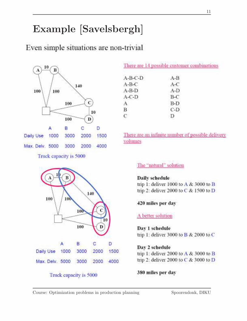
11

Example [Savelsbergh]


12

Deterministic Solution Method

From [Campbell and Savelsbergh (2004)]

Based on average product usage

2-phase Decomposition Approach

• Phase I: Planning (integer programming)

Determine which customers should receive a delivery on each

day of the planning and how much.

• Phase II: Scheduling (meta heuristic)

Create the precise delivery routes for each day.

Rolling horizon approach - execute j of a k-day plan

Decisions:

• When to serve a customer

• How much to deliver when serving

• Which delivery route to use


13

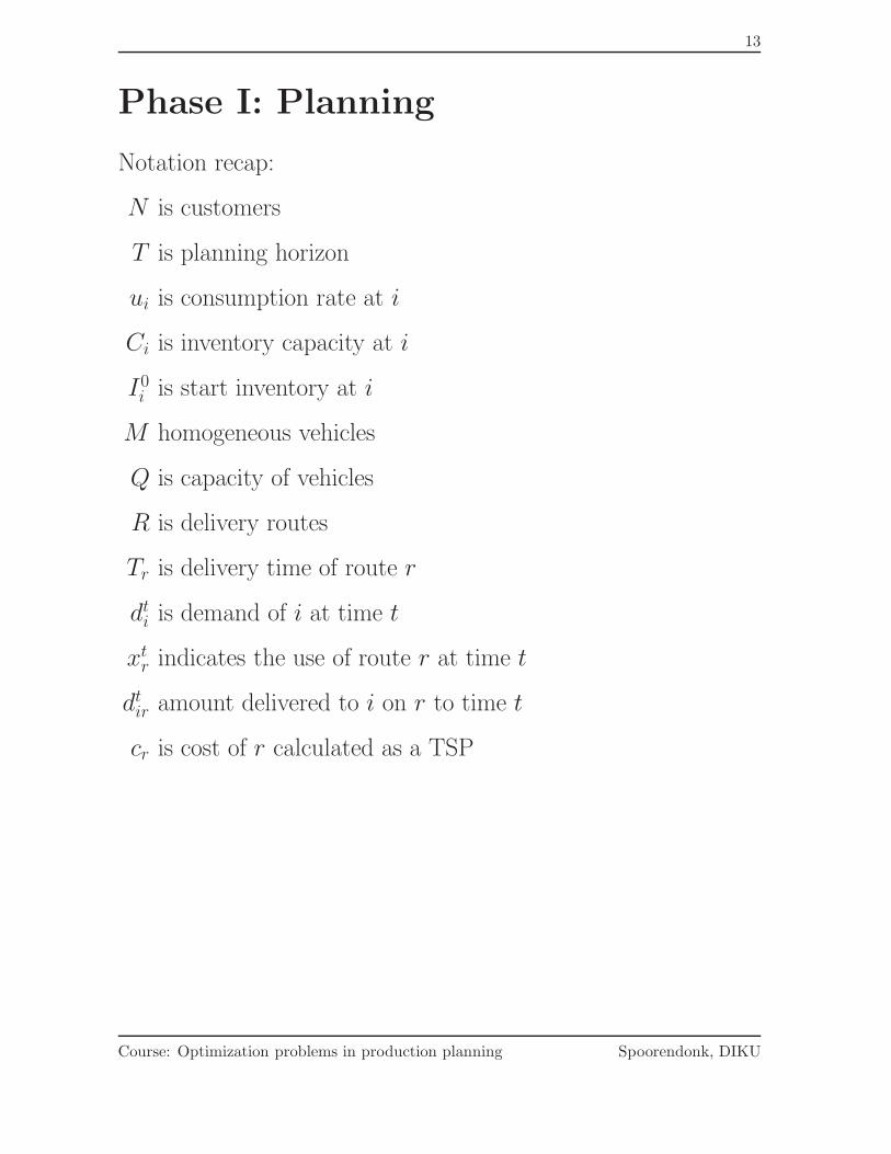
Phase I: Planning

Notation recap:

N is customers

T is planning horizon

ui is consumption rate at i

Ci is inventory capacity at i

I0i is start inventory at i

M homogeneous vehicles

Q is capacity of vehicles

R is delivery routes

Tr is delivery time of route r

dti is demand of i at time t

xtr indicates the use of route r at time t

dtir amount delivered to i on r to time t

cr is cost of r calculated as a TSP


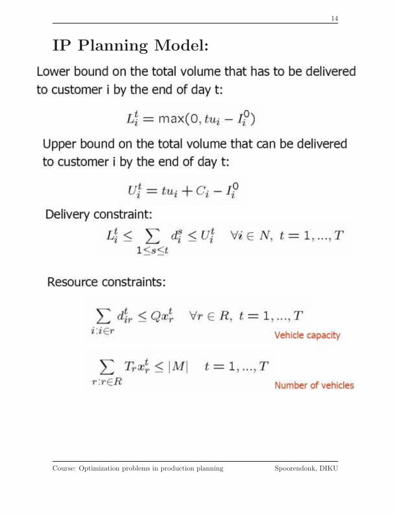
14

IP Planning Model:


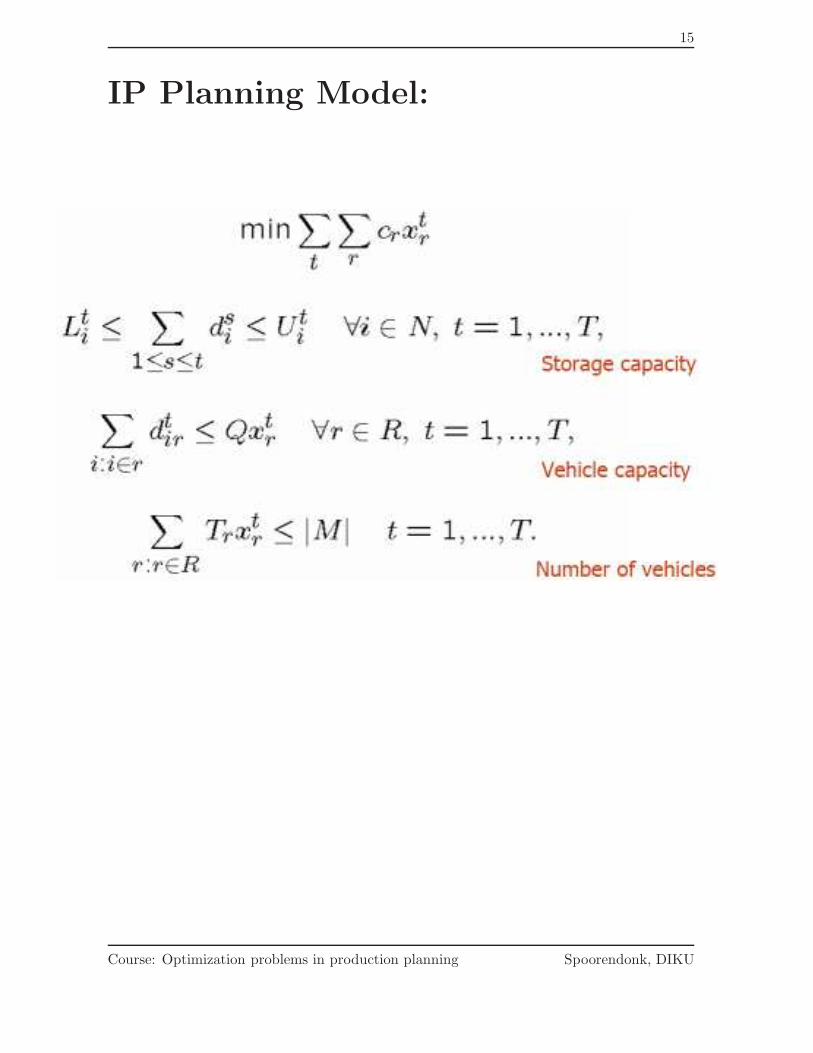
15

IP Planning Model:


16

Improve efficiency

Reduce number of delivery routes.

Clustering:

• Only customers in same cluster can be on same route

• Finding a good cluster:

1. Generate a large set of possible clusters based on distance

and size of delivery

2. Estimate the cost of serving each cluster. Depends on

location, consumption rate, and demand

3. solve a set partitioning problem to select cluster

• Done as preprocessing

Reducing customer sets:

• Critical customers, huge impact on scheduling

• Impending customers, require delivery soon

• Balance customers, added to balance routes including critical

or impending customers

Aggregation/Relaxation:

• Higher quality in beginning. Consider weeks instead of days

at end of planning period.


17

Phase II: Scheduling

Solve a VRPTW for each day.

Problem: Inflexible solutions.

Suggestion: j days insertion heuristic for scheduling routes.

Input for next j days:

• List of customers

• list of recommended delivery amounts

Output for next j days for each vehicle:

• Start time

• Sequence of deliveries

• Arrival time at each customer

• Actual delivery amount at each customer


18

Insertions

To keep low-order polynomial running time keep track of:

• Min and max delivery time for i

• Min and max delivery amount for i

Insertion score depends on several components:

1. Increased travel time

2. Forced waiting time due to delivery windows

3. Inflexible routes, e.g. small difference between delivery times

4. Inserting customers that are capable to be served by a full

truck load

Low scores are good.


19

Selection

• Check feasibility at each iteration

• Keep to lowest scores per delivery

• Always consider to put delivery on own route

Prioritize orders to avoid impossible insertions:

High Deliveries that must take place during the first j days

Low All other deliveries

Selection rules

1. If there are deliveries that cannot be inserted into a existing

route. Select the delivery with the most expensive route for

itself.

(Most expensive for itself leads to least expensive for other

uninserted.)

2. If all deliveries can be inserted into some route. Select the

delivery with largest difference between its two scores.

(Minimizing maximum regret.)

Embedded in a GRASP framework.


20

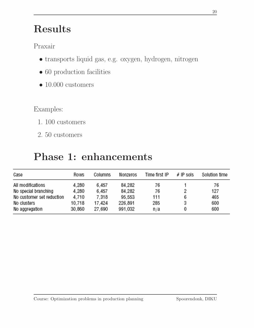
Results

Praxair

• transports liquid gas, e.g. oxygen, hydrogen, nitrogen

• 60 production facilities

• 10.000 customers

Examples:

1. 100 customers

2. 50 customers

Phase 1: enhancements


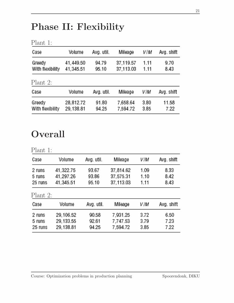
21

Phase II: Flexibility

Plant 1:

Plant 2:

Overall

Plant 1:

Plant 2:


22

Stochastic Solution Method

From [Kleywegt et al. (2002,2004)]

Based on probability distribution of product usage

Topics

• Formulated as a Markov Decision Process model

• Approximated with dynamic programming

Direct deliveries only, i.e., one vehicle per route.

Maximizing expected discounted value over an infinite time hori-

zon.

Notation:

cij cost of edge (i, j)

di amount delivered

ri(di) reward gained for delivery

si shortage

pi(si) penalty for shortage

xi amount in inventory

hi(xi + di) holding inventory cost


23

Markov Decision Process (MDP)

Models decision making in situations where outcome is partly

under random and partly under decision makers control.

• MDP is a discrete time stochastic control process character-

ized by states

• In each state the decision maker must choose between several

actions

• A transition function determines the transition probabilities

to the next state

• Each state possess the Markov property which means that is

state s of an MDP is known the transition to the next state

s + 1 is independent of previous states

Used for

• solving optimization problems with dynamic programming

• reinforcement learning

Areas

• robotics

• automated control

• economics

• manufacturing


24

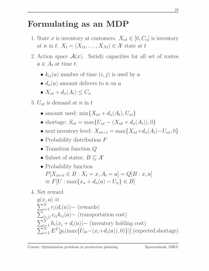
Formulating as an MDP

1. State x is inventory at customers. Xnt ∈ [0, Cn] is inventory

at n in t. Xt = (X1t, . . . , XNt) ∈ X state at t

2. Action space A(x). Satisfy capacities for all set of routes

a ∈ At at time t.

• kij(a) number of time (i, j) is used by a

• dn(a) amount delivers to n on a

• Xnt + dn(At) ≤ Cn

3. Unt is demand at n in t

• amount used: min{Xnt + dn(At), Unt}

• shortage: Snt = max{Unt − (Xnt + dn(At)), 0}

• next inventory level: Xnt+1 = max{Xnt+dn(At)−Unt, 0}

• Probability distribution F

• Transition function Q

• Subset of states: B ⊆ X

• Probability function

P [Xnt+t ∈ B : Xt = x, At = a] = Q[B : x, a]

≡ F [U : max{xn + dn(a) − Un} ∈ B]

4. Net reward

g(x, a) ≡∑N

i=1 ri(di(a))− (rewards)∑

(i,j) cijkij(a)− (transportation cost)∑N

i=1 hi(xi + di(a))− (inventory holding cost)∑N

i=1 EF [pi(max{Ui0−(xi+di(a)), 0)})] (expected shortage)


25

5. Objective function.

• Π policies depending on history up to t

• α ∈ [0, 1) discount factor

• Optimal value

V ∗(x) ≡ supπ∈Π

EF

[

∞∑

t=0

αtg(Xt, At) : X0 = 0

]

Stationary deterministic policy π proscribes decision π(x) ∈

A(x).

V π(x) ≡ EF

[

∞∑

t=0

αtg(Xt, π(Xt)) : X0 = 0

]

= g(x, π(X)) + α

∫

X

V π(y)Q[dy : x, π(x)]

Last is standard result in dynamic programming!

It suffices to consider stationary deterministic policies ΠSD.

V ∗(x) = supπ∈ΠSD

V π(x)

V ∗(x) = supπ∈ΠSD

V π(x

= supa∈A(x)

{

g(x, a) + α

∫

X

V ∗(y)Q[dy : x, a]

}

(1)


26

Solving The MDP

Recall:

V ∗(x) = supa∈A(x)

{

g(x, a) + α

∫

X

V ∗(y)Q[dy : x, a]

}

(1)

Determine optimal value V ∗ for optimal policy π∗.

1. Estimate V ∗ (lhs and rhs of (1)). Successive approximations

of V ∗(x) for x ∈ X (exponential size)

2. Estimate expected value (rhs of (1)). High dimensional inte-

gral. (dimensions equal number of customers)

3. Determine optimal action for each state. Solve maximization

problems (an IRP)

Shortcuts with Direct Deliveries

• Action space A(x) much smaller due to one customer per

route.

• Transportation cost per customer not on edges, i.e. cn and

kn(an) be the visits to n using a. Transportation cost is:

N∑

i=1

ciki(a)

Problem is still hard


27

Approximating the Value Function

Motivating observation:

• Net reward: g(x, a) =∑N

n=1 gn(xn, an)

• Probable inventory level function: qn(yn, kn : xn, dn), i.e.

probability that inventory is yn with kn visits given inventory

level xn and delivered amount dn the day before.

Decompose into customer subproblems:

1. State (xn, kn)

2. Action A(xn, kn) constrained by vehicle and inventory ca-

pacity

3. Transition properties

P [(Xnt+1, Knt+1) = (yn, ln) : (Xnt, Knt) = (xn, kn), Ant = an] =

qn(yn, kn : xn, dn(an))

4. Net reward gn(xn, an)

5. Objective is to maximize

V ∗(xn, kn) = sup{Ant}

∞t=0

E

[

∞∑

t=0

αtgn(Xnt, Ant) : (Xno, Kn0) = (xn, k0)

]


28

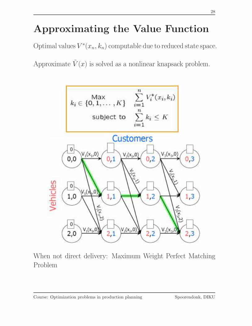
Approximating the Value Function

Optimal values V ∗(xn, kn) computable due to reduced state space.

Approximate V (x) is solved as a nonlinear knapsack problem.

When not direct delivery: Maximum Weight Perfect Matching

Problem


29

Estimation of the Expected Value andOptimal Action

Randomized algorithm to estimate expected value of an action.

[Nelson-Matecjik]

Many possible actions. Computational inefficient to con-

sider all actions.

Greedy algorithm to identify good actions for all states.

Speed ups

Use parametric functions when approximating value function.

Random sampling and variance reduction techniques when esti-

mating integral.


30

Results

Policies to assign vehicles:

CBW [Chien, Balakrishnan and Wong] IP to make single-day

plans. Long term effect passed to next day.

Myopic Greedily assigns vehicles to customers.

KNS1 Decomposition approximation

KNS2 Parametric decomposition approximation

Conclusions

• KNS2 performs best but gains less when instances grow in

size

• Dynamic Programming Approximate methods are viable


Documents

inventory routing - diku.dk · PDF fileInventory Routing Course: Optimization problems in production planning Simon Spoorendonk DIKU, ... Conventional Inventory Management Customer: