Mathematical Model for Maritime Inventory Routing Problem with Multiple Time Windows

Nurhadi Siswanto Industrial Engineering Department

Institut Teknologi Sepuluh Nopember Surabaya, Indonesia

siswanto@ie.its.ac.id; nurhadi.siswanto@gmail.com

Abstract—This paper considers a new variant of the maritime inventory routing problem which considers multiple time windows. The typical time windows that this problem considers that it may exist for certain ports which only permit a ship entering and leaving the ports within daytime due to both natural conditions and their facilities. A mathematical model formulated as mixed integer programming is developed for solving this kind of problem. The problem is to find how many products and how much of each products are carried by each ship from source ports which assumed have constant production rates to destination ports which assumed have constant consumptions rates without exceeding the production port storages and out of stocks in the consumption port storages during the planning horizon. The objective of the problem is to minimize the cost while satisfying a set of technical and physical constraints. The detailed modified variables and constraints from the ones exist in the literature are discussed. Then the model is tested with several test problems with different days of planning horizon as well as different number of ship visits at consumption ports during planning horizon. The experiment results solved using LINGO show that modeling multiple time windows can give higher objective functions in comparison to the ones of without time windows. Moreover, modeling multiple time windows significantly increases the computational time in comparison with the ones without multiple time windows.

Keywords—mathematical model, maritime, inventory routing problem, multiple time windows

I. INTRODUCTION

This paper presents methods to solve the maritime inventory routing problem with multiple time windows. The problem is motivated by the desire to more closely modeling the real world problem faced by a national oil company in the South East Asia region. This problem is similar to that in [1], except that it now considers that the ports that are served by the ships vary due to each port’s natural conditions and facilities. For example, some ports are small with incomplete facilities. In these ports, ships may only shift in and out from the ports during daytime. This means that a time window may exist, and hence this corresponds to a problem with multiple time windows during a predefined planning horizon.

It is relatively difficult to find papers that discuss multiple time windows. The few papers in the literature which discuss this problem are [2], [3], [4], and [5]. All of these, except [4], focus on the routing problem without considering inventory constraints. Christiansen and Fagerholt [2] discuss a ship scheduling problem for pick-up and delivery of bulk cargoes. In addition to the lack of inventory constraints, their problem assumes that the ports are not available for service at night and during weekends. In contrast, this paper’s problem only restricts in that a ship can only enter or leave some ports during daytime. However, once a ship is in a port, a loading/unloading service will not be interrupted until the process is finished.

Favaretto, Moretti, and Pellegrini [3] discuss a generic vehicle routing problem, not inventory routing problem, where customers have multiple time windows and may be visited several times during a predefined planning horizon. They formulated a mathematical model of such problems and proposed to solve them by using the ant colony method. Furthermore, Tricoire, Romauch, Doerner, and Hartl [5] presents a multi-period orienteering problem to routing and scheduling sales representatives, which visit their customers according to certain multiple time windows which exist for each customer. The problem categorized the customers into mandatory and optional customers. Each customer in the first category must be visited exactly once while the second category is optional. This paper is also not considered as inventory routing problem. They proposed to solve this by using an exact method, which had embedded within it a sub-process, that they called a variable neighbourhood search.

Doerner, Gronalt, Hartl, Kiechle, and Reimann [4] also discuss the vehicle routing problem, but where multiple time windows are interdependent. In that, the prior pickup time determines the next visit for each particular customer. There also exists inventory constraints that must be considered when calculating the next visit, therefore, unlike the other above papers, this paper can be categorised as an inventory routing problem (IRP), because the customer may be visited more than one. In [4], repeated visits may be necessary to avoid products perishing, while this paper must maintain storage levels within their limits. Unlike this paper’s problem that considers several non-mixable products, Doerners’ paper only concerned one product (or several mixable products) to be picked up. This means, in their problem, there is no need for an assignment method to allocate products into compartments. Moreover, they assume that service time is fixed. In this paper’s problem, the service

2767© IEOM Society International

Proceedings - International Conference on Industrial Engineering and Operations Management, Kuala Lumpur, Malaysia, March 8-10, 2016

(loading/unloading process) time depends on the quantities loaded or unloaded. Also, there exists a fixed setup time for changing products in this paper’s model.

As defined in [1], an IRP that uses ships to distribute product(s) can be categorized as a maritime inventory routing problem (mIRP). Many papers have discussed this problem, for example [6], [7], [8], [9] and [10]. However these mIRP papers do not include daily operational port’s time windows in their model. The study of the multiple time windows problem is interesting both in theory and practice, as many problems can have this situation, not only in maritime, but also in land transportation scenarios.

II. MATHEMATICAL MODEL In modeling this kind of mIRP with multiple time windows, we refer to [1]. There are several variables that must be

used in addition to those that have been discussed in our previous research. The first two variables are slimk and tl

im, which represent the level of product k at the time when a ship leaves and the time of the ship when it leaves, from node (i,m), respectively. The variable tl

im is added to the model because ships must leave the port within its operational time windows, while sl

imk is added to maintain that at the time of the ships’ leaving, that the levels of the port’s storages are within their lower and upper limits.

The other new variables are toimd, ti

imd, tpoimd, and tpi

imd. These variables are related to modeling the multiple time windows. These variables are not continuous as shown in Fig.1. If discrete time modeling is used instead, it is not difficult to formulate the multiple time windows, because the model has an explicit time indicator. The constraints TWS

id ≤ t im ≤ TWFid and

TWSid ≤ tl im ≤ TWF

id can be used to bound that the arrival and leaving time must be within the time windows of ports. Unlike for discrete time modeling, the continuous time modeling does not have an explicit time signal. In this kind of modeling the time signal is represented by a pair of port number (i) and the sequence ship’s visit number at that port (m), called as a node (i,m). The new variables are used to enforce that ships must enter and leave certain ports within their time windows. The detailed modeling are as follow.

A. Notations In modeling multiple time windows, there are several parameters and variables that must be used for this problem in

addition to those that have been discussed in [1]. The subscripts are defined as follow: i, j the port M the number of ships visited a port mp the number of ships visited a production port mc the number of ships visited a consumption port

(i,m) a node represents the number of ships visited port i V the ship K the product C the compartment D the day

The complete parameters are:

CMvc the maximum capacity of the compartment c of ship v COik the loading (or unloading) setup cost of product k at port i CTijv the traveling cost of ship v from port i to port j CWiv the setup cost of ship v at port i ISik initial inventory of product k at port i Jik equal to 1 if port i is a producer of product k, and equal to -1 if it is a consumer Ni the maximum number of visits of ships at port Hi∈

QQvkc the initial quantity of product k loaded in compartment c of ship v Rik the production (or consumer) rate of product k at port i

SMik the minimum level of product k at port i SXik the maximum level of product k at port i TBi the duration between the departure of one ship and the arrival of the next ship TH the planning horizon

TOik loading (or unloading) setup time of product k at port i TSE

iv setup time before loading (or unloading) activity of ship v at port i TSL

iv setup time of ship v before leaving from port i TQik the loading (or unloading) rate of one unit of product k at port i TTijv the traveling time of ship v from port i to port j

2768© IEOM Society International

Proceedings - International Conference on Industrial Engineering and Operations Management, Kuala Lumpur, Malaysia, March 8-10, 2016

TWi the setup time at port i TWS

id the start of time window of port i at day d TWF

id the end of time window of port i at day d The variables are as follow:

limvkc the quantity of product k onboard loaded in compartment c of ship v after departing from node (i,m) oimvkc equal to 1 if ship v visits node (i,m) and loads (or unloads) product k into (or from) compartment c,

otherwise 0 ppimvk equal to 1 if there is loading or unloading of product k to or from any compartments of ship v at node

(i,m) qimvkc the quantity of product k loaded (or unloaded) into (or from) compartment c of ship v at node (i,m) simk the level of product k at the time when a ship arrives at node (i,m). tim the arrival time of a ship at node (i,m)

tweim entering waiting time of a ship visits at node (i,m)

twlim leaving waiting time of a ship from node (i,m)

wimv equal to 1 if ship v visits node (i,m) and performs port setup, otherwise 0 ximjnv equal to 1 if ship v travels from node (i,m) to node (j,n), otherwise 0 yim equal to 1 if node (i,m) is not visited by any ships, otherwise 0 zimv equal to 1 if ship v finishes its route at node (i,m) , otherwise 0 sl

imk the level of product k at the time when a ship leaves from node (i,m). tl

im the departure time of a ship from node (i,m) to

imd semi continuous variable that have values of either zero or the same as tlim

tiimd semi continuous variable that have values of either zero or the same as tim

tpiimd equal to 1 if a ship visits node (i,m) in day d

tpoimd equal to 1 if a ship leaves node (i,m) in day d

The last six variables which are specifically being used for this problem influence some constraints as in [1]. Routing

constraints do not change, neither do the loading and unloading constraints. However, the scheduling and inventory constraints have changed significantly, so they will be explained in detail below.

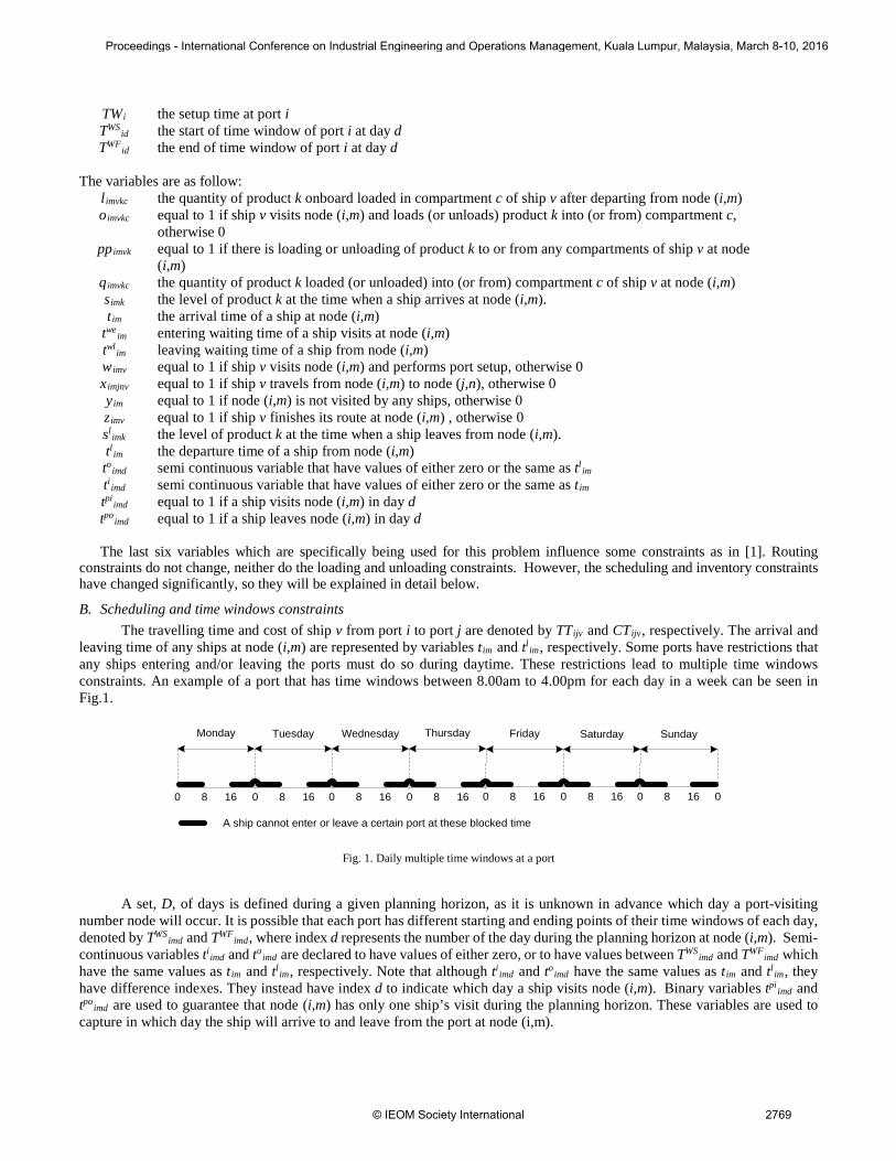
B. Scheduling and time windows constraints The travelling time and cost of ship v from port i to port j are denoted by TTijv and CTijv, respectively. The arrival and

leaving time of any ships at node (i,m) are represented by variables tim and tlim, respectively. Some ports have restrictions that any ships entering and/or leaving the ports must do so during daytime. These restrictions lead to multiple time windows constraints. An example of a port that has time windows between 8.00am to 4.00pm for each day in a week can be seen in Fig.1.

Monday Tuesday ThursdayWednesday

0 8 16 0 8 16 0 8 16 0 8 16

Friday Saturday Sunday

0 8 16 0 8 16 0 8 16 0

A ship cannot enter or leave a certain port at these blocked time

Fig. 1. Daily multiple time windows at a port

A set, D, of days is defined during a given planning horizon, as it is unknown in advance which day a port-visiting

number node will occur. It is possible that each port has different starting and ending points of their time windows of each day, denoted by TWS

imd and TWFimd, where index d represents the number of the day during the planning horizon at node (i,m). Semi-

continuous variables tiimd and to

imd are declared to have values of either zero, or to have values between TWSimd and TWF

imd which have the same values as tim and tl

im, respectively. Note that although tiimd and to

imd have the same values as tim and tlim, they

have difference indexes. They instead have index d to indicate which day a ship visits node (i,m). Binary variables tpiimd and

tpoimd are used to guarantee that node (i,m) has only one ship’s visit during the planning horizon. These variables are used to

capture in which day the ship will arrive to and leave from the port at node (i,m).

2769© IEOM Society International

Proceedings - International Conference on Industrial Engineering and Operations Management, Kuala Lumpur, Malaysia, March 8-10, 2016

When a ship does not arrive within the port’s time window, the ship must wait. A continuous variable tweim is declared

as the entering waiting time of a ship at node (i,m). If the time of when a ship arrives is inside the time window, the ship can directly lay into the port and there is no waiting time. Therefore, the value of twe

im is zero. In the same way, a ship must also leave from certain ports within their time windows. The duration of the leaving waiting time of the ship at node (i,m) is denoted as twl

im. At certain ports, there is also a restriction that only one ship at a time can lay in it. So, if there is another ship in the port,

the ship must wait to enter it. The variable tweim is used to model this waiting time. A parameter TB

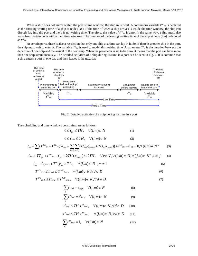
i is the duration between the departure of one ship and the arrival of the next ship. When the parameter is set to be zero, it means that the port can have more than one ship simultaneously. The detailed activities of a ship during its time in a port can be seen in Fig. 2. It is common that a ship enters a port in one day and then leaves it the next day

Waiting time to enter the port

Setup time before loading/

unloading

TSEiv

Waiting time to leave the port

Setup time before leaving

TSLiv

Loading/Unloading Activities

Lay Time

Port’s Time

Variabletwe

im

The time of when a ship lays

in

The time of when a ship lays

off

Variabletwl

im

The time of when a

ship arrives at

a port

Fig. 2. Detailed activities of a ship during its time in a port

The scheduling and time windows constraints are as follows:

NmiTHtim ∈∀≤≤ ),(,0 (1)

NmiTHt iml ∈∀≤≤ ),(,0 (2)

Lim

lim

wlimvkcik

Pk Ccimvkcikimviv

SLiv

SEim NmittoTOqTQwTTt

v v

∈∀=−+++++∑ ∑∑∈ ∈

),(,0))()( (3)

jiNnjNmiVvTHxTHttTTt Limjnvjnim

weijvim

l ≠∈∀∈∀∈∀≤+−++ ,),(,),(,,2)(2 (4)

1,),(,)1( ≠∈∀≥+− − mNmiTyTtt Li

Bimi

Bmi

lim (5)

DdNmiTtT imdWF

imdi

imdWS ∈∀∈∀≤≤ ,),(, (6)

DdNmiTtT imdWF

imdo

imdWS ∈∀∈∀≤≤ ,),(, (7)

Nmitt imd

imdi ∈∀=∑ ),(, (8)

Nmitt iml

dimd

o ∈∀=∑ ),(, (9)

DdNmitTHt imdpi

imdi ∈∀∈∀≤ ,),(, (10)

DdNmitTHt imdpo

imdo ∈∀∈∀≤ ,),(, (11)

Nmitd

imdpi ∈∀=∑ ),(,1 (12)

2770© IEOM Society International

Proceedings - International Conference on Industrial Engineering and Operations Management, Kuala Lumpur, Malaysia, March 8-10, 2016

Nmitd

imdpo ∈∀=∑ ),(,1 (13)

Constraints (1)-(2) restrict the arrival and leaving time of a ship within the planning horizon. Constraint (3) calculates the

arrival and leaving time of a ship in one node, while constraint (4) tracks the routing time from a node to another node. Constraint (5) ensures that the time precedence constraints are not violated. This constraint restricts a port to only have another ship after a particular period of time. Constraints (6)-(7) enforce that a ship enters and leaves a port within its time windows. Constraints (8)-(9) set the time of when a ship arrives and leaves at the particular day and time when it arrives and leaves node (i,m). Constraints (10)-(11) are used to determine in which day a ship arrives and leaves a port. Finally, constraints (12)-(13) guarantee that only one day occurs for each of arriving and leaving at node (i,m).

C. Inventory constraints There are four parameters that are related to the inventory constraints. QQik defines an initial inventory of product k at port

i. The maximum and minimum level of product k at port i are represented by SMik and SXik, respectively. Rik is the production (or consumption) rate of product k at port i. These variables are related to the inventory constraints: s imk and sl

imk, which represents the level of product k at the time when a ship arrives and leaves at node (i,m), respectively. The inventory constraints are as follow:

vvP

imiml

ikikimkimvkc CcPkNmiVvttRJsq ∈∀∈∀∈∀∈∀−+≤ ,,),(,],[ (14)

PkNmitRJQQs Piikikikki ∈∀∈∀+= ,),(,11 (15)

1,),,(,0)( )1()1( ≠×∈∀=−−+ −− mKNkmisttRJs iimkmil

imikikkmil (16)

( ) 1,),,(,0)( ≠×∈∀=−−+−∑∑∈ ∈

mKNkmisttRJqJs iimkl

Vv Ccimim

likikimvkcikimk

v v

(17)

iikimkik KNkmiSXsSM ×∈∀≤≤ ),,(, (18)

iikimkl

ik KNkmiSXsSM ×∈∀≤≤ ),,(, (19)

iX

iikiml

ikikimkl

ik MmKNkmiSXtTHRJsSM =×∈∀≤−+≤ ,),,(,)( (20)

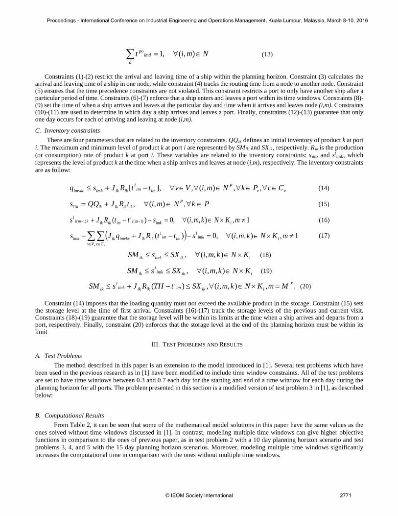
Constraint (14) imposes that the loading quantity must not exceed the available product in the storage. Constraint (15) sets the storage level at the time of first arrival. Constraints (16)-(17) track the storage levels of the previous and current visit. Constraints (18)-(19) guarantee that the storage level will be within its limits at the time when a ship arrives and departs from a port, respectively. Finally, constraint (20) enforces that the storage level at the end of the planning horizon must be within its limit

III. TEST PROBLEMS AND RESULTS

A. Test Problems The method described in this paper is an extension to the model introduced in [1]. Several test problems which have

been used in the previous research as in [1] have been modified to include time window constraints. All of the test problems are set to have time windows between 0.3 and 0.7 each day for the starting and end of a time window for each day during the planning horizon for all ports. The problem presented in this section is a modified version of test problem 3 in [1], as described below:

B. Computational Results From Table 2, it can be seen that some of the mathematical model solutions in this paper have the same values as the

ones solved without time windows discussed in [1]. In contrast, modeling multiple time windows can give higher objective functions in comparison to the ones of previous paper, as in test problem 2 with a 10 day planning horizon scenario and test problems 3, 4, and 5 with the 15 day planning horizon scenarios. Moreover, modeling multiple time windows significantly increases the computational time in comparison with the ones without multiple time windows.

2771© IEOM Society International

Proceedings - International Conference on Industrial Engineering and Operations Management, Kuala Lumpur, Malaysia, March 8-10, 2016

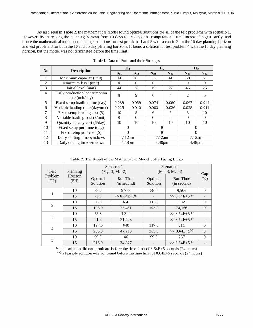
As also seen in Table 2, the mathematical model found optimal solutions for all of the test problems with scenario 1. However, by increasing the planning horizon from 10 days to 15 days, the computational time increased significantly, and hence the mathematical model could not get solutions for test problems 1 and 5 with scenario 2 for the 15 day planning horizon and test problem 3 for both the 10 and 15 day planning horizons. It found a solution for test problem 4 with the 15 day planning horizon, but the model was not terminated before the time limit.

Table I. Data of Ports and their Storages

No Description H1 H2 H3 S11 S12 S21 S22 S31 S32

1 Maximum capacity (unit) 160 180 55 41 68 51 2 Minimum level (unit) 0 0 0 0 0 0 3 Initial level (unit) 44 28 19 27 46 25 4 Daily production/ consumption

rate (unit/day) 8 9 6 4 2 5

5 Fixed setup loading time (day) 0.039 0.059 0.074 0.060 0.067 0.049 6 Variable loading time (day/unit) 0.025 0.010 0.003 0.026 0.028 0.014 7 Fixed setup loading cost ($) 10 8 6 9 8 10 8 Variable loading cost ($/unit) 0 0 0 0 0 0 9 Quantity penalty cost ($/day) 10 10 10 10 10 10

10 Fixed setup port time (day) 0 0 0 11 Fixed setup port cost ($) 0 0 0 12 Daily starting time windows 7.12am 7.12am 7.12am 13 Daily ending time windows 4.48pm 4.48pm 4.48pm

Table 2. The Result of the Mathematical Model Solved using Lingo

Test Problem

(TP)

Planning Horizon

(PH)

Scenario 1 (Mp=3; Mc=2)

Scenario 2 (Mp=3; Mc=3) Gap

(%) Optimal Solution

Run Time (in second)

Optimal Solution

Run Time (in second)

1 10 38.0 9,787 38.0 9,506 0 15 73.0 >> 8.64E+5(ⁿ) - >> 8.64E+5(*) -

2 10 66.8 656 66.8 582 0 15 103.0 25,451 103.0 74,166 0

3 10 55.8 1,329 - >> 8.64E+5(*) - 15 91.4 21,423 - >> 8.64E+5(*) -

4 10 137.0 640 137.0 211 0 15 265.0 47,210 265.0 >> 8.64E+5(ⁿ) 0

5 10 99.0 46 99.0 267 0 15 216.0 34,827 - >> 8.64E+5(*) -

(ⁿ) the solution did not terminate before the time limit of 8.64E+5 seconds (24 hours) (*) a feasible solution was not found before the time limit of 8.64E+5 seconds (24 hours)

2772© IEOM Society International

Proceedings - International Conference on Industrial Engineering and Operations Management, Kuala Lumpur, Malaysia, March 8-10, 2016

IV. CONSLUSION

In this paper, a new variant of inventory routing problem is considered. The problem is an extension of the work in the area in that the problem considers a ship that can only enter and leave the ports within their time windows during planning horizon. A mathematical model is formulated as mixed integer programming for solving this problem. A set of new parameters, new variables and modified constrainst, especially scheduling and time windows constraints and inventory constraints are discussed. The objective of the problem is to find a minimum cost solution while satisfying a number of technical and physical constraints within a given planning horizon. Several problem instances are created due to uniqueness of the problem. The test results on problem instances show that the longer planning horizon the higher objective function and the longer computational time. This excessive running time was a major motivation for our next research agenda, developing a heuristic method.

REFERENCES [1] N. Siswanto, D. Essam, R. Sarker, “Solving the ship inventory routing and scheduling problem with undedicated compartments”

Computers and Industrial Engineering, vol. 61, pp. 289-299, September 2011.[2] M. Christiansen, K. Fagerholt,”Robust ship scheduling with multiple time windows”, Naval Research Logistics, vol. 49(6), pp. 611-

625, August 2002.[3] D. Favaretto, E. Moretti, P. Pellegrini, “Ant colony system for a vrp with multiple time windows and multiple visits”, Journal of

Interdisciplinary Mathematics, vol. 10 (2), pp. 263-284, 2007.[4] K.F. Doerner, M. Gronalt, R.F. Hartl, G. Kiechle, M. Reimann, “Exact and heuristic algorithms for the vehicle routing problem with

multiple interdependent time windows”, Computers and Operations Research, vol. 35 (9), pp. 3034-3048, September 2008.[5] F. Tricoire, M. Romauch, K.F. Doerner, R.F. Hartl, “Heuristics for the multi-period orienteering problem with multiple time windows”,

Computers and Operations Research, vol. 37 (2), pp. 351-367, February 2010.[6] F. Al-Khayyal, S.J. Hwang,”Discrete Optimization-Inventory constrained maritime routing and scheduling for multi-commodity liquid

bulk, Part I: Applications and model”, European Journal of Operational Research, vol. 176, pp. 106–130, January 2007.[7] M. Christiansen, B. Nygreen, “A method for solving ship routing problems with inventory constraints”, Annals of Operations Research,

vol. 81, pp. 357-378, June 1998.[8] M. Christiansen, B. Nygreen, “Modeling path flows for a combined ship routing and inventory management problem”, Annals of

Operations Research, vol. 82, pp. 391-413, August 2998.[9] M. Christiansen, “Decomposition of a combined inventory and time constrained ship routing problem”, Transportation Science, vol. 33

(1), pp. 3-16, February 1999.[10] S.J. Hwang, “Inventory Constrained Maritime Routing and Scheduling for Multi-Commodity Liquid Bulk”, Thesis (Unplublished),

School of Industrial and Systems Engineering, Georgia Institute of Technology, April 2005.

BIOGRAPHY Nurhadi Siswanto is currently the Head of Industrial Engineering Department at Institut Teknologi Sepuluh Nopember, Surabaya, Indonesia. He holds a Bachelor of Science degree in Industrial Engineering from Institut Teknologi Sepuluh Nopember, Surabaya, Indonesia, Master of Science in Industrial Engineering (MSIE) from Purdue University, West Lafayette, Indiana, USA and PhD in Computer Science with specialisation in Operation Research from University of New South Wales (UNSW), Canberra, Australia. His research interests includes large scale optimization and simulation modeling, and also maritime transportation. He has been involved consultancy activities in several companies, such as Pertamina, Garuda Indonesia, Semen Indonesia and Petrokimia Gresik.

2773© IEOM Society International

Proceedings - International Conference on Industrial Engineering and Operations Management, Kuala Lumpur, Malaysia, March 8-10, 2016