Inventory, Price, and Output in the Linerboard Industry

Haizheng Li &

Feng Zhang

School of Economics, Georgia Institute of Technology Atlanta, GA 30332-0615, USA

Phone: 404-894-3542 E-mail: haizheng.li@econ.gatech.edu

February, 2006

________________________ * This research was sponsored by the Center for Paper Business and Industry Studies (CPBIS), one of twenty-two Industry Centers funded by the Sloan Foundation. All of the opinions expressed in this paper are attributed to the authors and are not those of CPBIS or the Sloan Foundation. We thank Patrick McCarthy, James McNutt, Colleen Walker, Jifeng Luo and Lei Lei for helpful suggestions, and Kevin Mabe for editing the English. All errors and omissions remain the responsibility of the authors.

1

ABSTRACT

In this study, we investigate the market dynamics in the linerboard industry.

Using discrete choice modeling techniques, we estimate the probability of price and

production response to inventory changes based on monthly data from 1980 to 1999. Our

tests show that inventory causes changes in price, but not vice versa. Moreover, price

responses to inventory are asymmetric, and upward adjustment in price is “stickier” than

downward adjustment. In contrast, production is found to lead inventory change, but a

reverse causal relationship exists. It appears that the industry cuts output in response to

inventory pressure, but the response seems to be temporary. Moreover, price drops

earlier in response to inventory buildup and output drops much later. There seems to be a

tendency for the industry to adjust price first before adjusting output. The output

adjustment seems to be short-lived and thus does not help remove the price pressure.

1

1. INTRODUCTION

It is well-known that the market equilibrium price and output is determined in a

complicated demand/supply system, influenced by the particular market structure. For

industry players, however, the adjustment process of output and price in response to

economic shocks is of greater interest than the equilibrium itself. Understanding the

adjustment dynamics will have important implications for production planning and

inventory management.

In this study, we investigate the short-term dynamics between price, output and

inventory in the US linerboard industry. Using both a linear probability model (LPM)

and a probit model, we estimate the short-term adjustment of price and output in response

to inventory changes. The models provide estimated probabilities of increase or decrease

in price and output, given the level of inventory in the previous period. Our results shed

some light on the behavior of firms in the linerboard industry in response to economic

shocks. We can gain some insight into the degree of price and output flexibility in

response to market conditions and industry climate. Additionally, the models can be used

to predict the probabilities of future changes in price and output, and thus help production

planning.

There have been numerous studies on the interactions between inventory, price

and output. For example, Blinder (1983) investigates the relationship between

inventories and sticky prices, and find that both price and output responses become

smaller as demand shocks become less persistent and output becomes more

“inventoriable.” Aguirregabiria (1999) examines the interaction between price and

inventory decisions in retailing firms and its implications for the dynamics of markups

2

and the existence of sales promotions. Using panel data of a supermarket chain and a

fixed effects probit model, the study shows that inventory has a significant effect on the

probability of retail price adjustments. When the inventory is large, the firm tends to

reduce the retail price, but when the inventory starts to decrease price increases become

more likely.

There are very few studies on short term market dynamics in the pulp and paper

industry. Dagenais (1976) presents a model of price determination for newsprint in North

America and shows that the necessity for the price leader to lower prices in times of

lower operating rate, in order to prevent excessive temptation for other mills to undersell.

Booth, et al (1991) find that, in the North American news print industry, prices are

determined using either a mark-up over marginal cost or adjusted full-cost. Buongiorno

and Lu (1989) show that a mark-up pricing model has given plausible results for U.S.

data with an inventory-output ratio variable serving as the signal for price change.

Christensen and Caves (1997) analyze the structural conditions governing investment

rivalry in the North American pulp and paper industry. Their OLS estimation shows that

prices vary closely with short-run marginal costs when capacity utilization is below 93

percent but rise rapidly as capacity grows more fully utilized.

This study adds to the short list of research for the pulp and paper industry by

investigating the short-term market dynamics in the linerboard industry. We estimate the

probability of changes in price and output in response to inventory level in the previous

months. The rest of the paper is organized as follows. In Section 2, we describe the data

and summary statistics. Section 3 outlines a simple theoretical framework for price and

output adjustment. Section 4 provides the results on causality tests. In Section 5, we

3

discuss price adjustment based on LPM estimation and Probit estimation. Section 6

discusses the output adjustment, and Section 7 concludes.

2. THE DATA

We use monthly data from January, 1980 to December, 1999, obtained from

‘AFPA Statistics for Time Series Analysis: 1980-1999’ (United States, 2000). The

linerboard price is the transaction price per short ton for 42lb unbleached Kraft linerboard,

taken from different issues of the Official Board Markets. The Official Board Markets

publishes three different prices for every period: the minimum, the maximum and the

simple average price. We use the average price. The inventory data include inventory at

linerboard mills and box plants.

We define a qualitative measure of price and output movement; i.e., if price rises

relative to the previous period, we defined price change as 1, and 0 otherwise. The

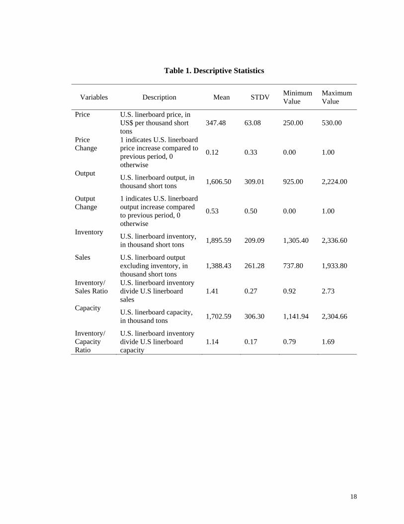
output change is defined similarly. Descriptive statistics are reported in Table 1. As can

be seen, price increased for only 12% of the period. Output increases occurred much

more frequently, about 53% of the time. On average, inventory is about 1.41 times the

total sales, and about 1.14 times the capacity. The lowest inventory level is about 92% of

the total sales but the highest level is about 273% of the sales.

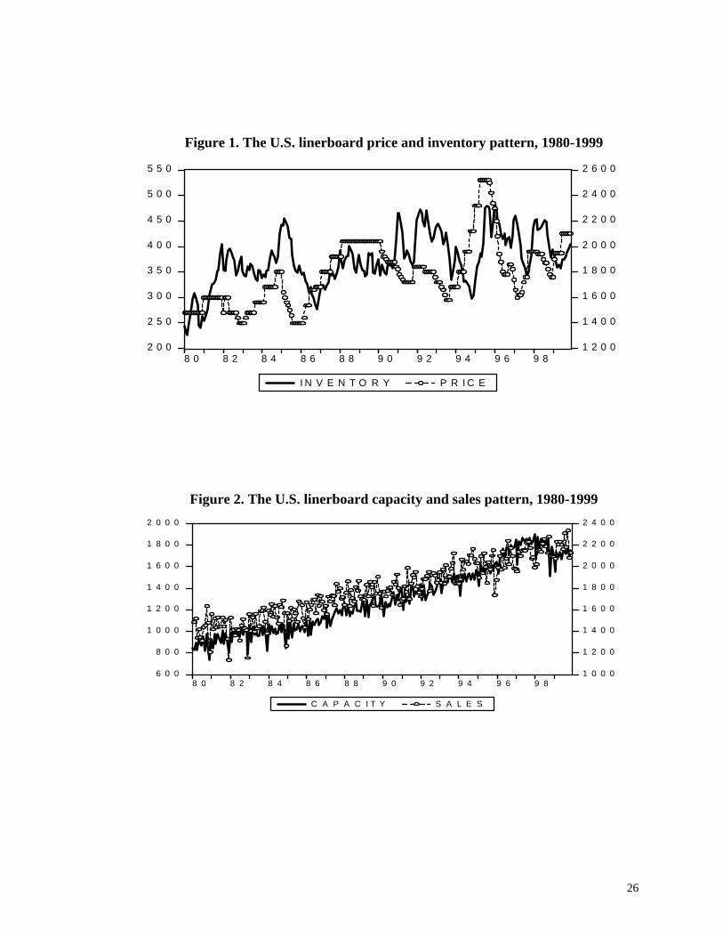
Figure 1 displays U.S. linerboard price and inventory levels. It appears that those

two series move together with a clear pattern of negative correlation; i.e., when inventory

declines, price tends to go up, and vice versa. It also shows that inventory somewhat

leads the change. The inventory level seems to have an increasing trend since 1980.

However, the rising inventory level may be simply caused by the rising output or

4

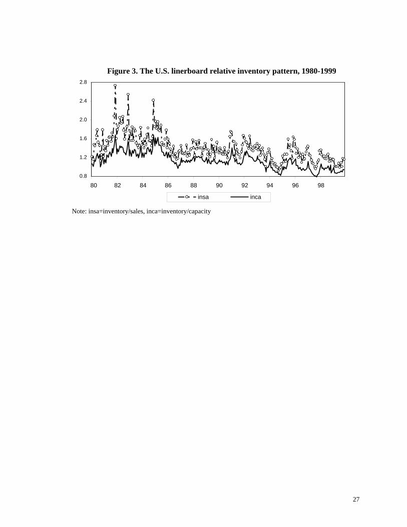
capacity. As shown in Figure 2, industry capacity and sales have risen consistently since

1980. Therefore, we also measure relative inventory level by its ratio to sales and

capacity. Figure 3 shows the trend of relative inventory to sales and capacity. The

relative inventory is the highest in the period from 1982 to 1985. Since then, both ratios

have shown a downward trend, indicating that the overall stock of relative inventory has

been declining in the linerboard industry.

3. A SIMPLE THEORETICAL FRAMEWORK

In the U.S. paper and paperboard industry, the level of concentration measured by the

share of top four producers is in the moderate range of 35-40%. A few existing studies for the

paper and paperboard industry indicate the existence of an oligopolistic structure. For instance,

Rich (1983) describes the process of price determination in paper and paperboard industries as

“target-return pricing, tempered by marginal cost pricing”. That is, prices are set on a target

return basis during periods of strong demand but approach the marginal cost during periods of

weak demand. Buongiorno and Lu (1989) find that increases in inventory-output ratios always

lead to decreases in prices, which supports the hypothesis of mark-up pricing behavior in pulp

and paper industries. In the linerboard industry, given the low level of concentration, it is

difficult for any of the firms to be an effective price leader.

Based on the economic theory, price is determined by the demand and supply

structure. Li and Luo (2005) estimate the supply/demand system for the linerboard

industry and provide a number of price and output elasticities. In this study, we focus on

the short-term price and output adjustment in response to inventory changes. We specify

the demand and supply functions for the U.S. paper and paper board industry as follows,

(1) ttt PD εβ +=

5

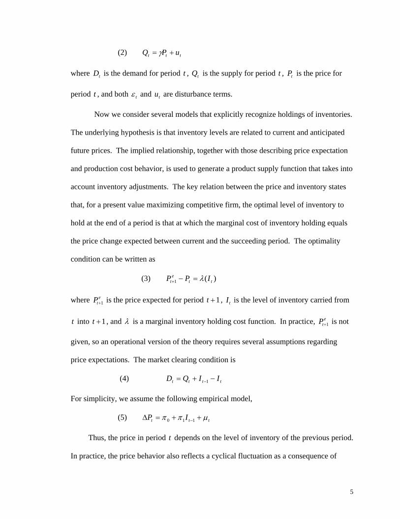
(2) ttt uPQ += γ

where tD is the demand for period t , tQ is the supply for period t , tP is the price for

period t , and both tε and tu are disturbance terms.

Now we consider several models that explicitly recognize holdings of inventories.

The underlying hypothesis is that inventory levels are related to current and anticipated

future prices. The implied relationship, together with those describing price expectation

and production cost behavior, is used to generate a product supply function that takes into

account inventory adjustments. The key relation between the price and inventory states

that, for a present value maximizing competitive firm, the optimal level of inventory to

hold at the end of a period is that at which the marginal cost of inventory holding equals

the price change expected between current and the succeeding period. The optimality

condition can be written as

(3) )(1 tte

t IPP λ=−+

where etP 1+ is the price expected for period 1+t , tI is the level of inventory carried from

t into 1+t , and λ is a marginal inventory holding cost function. In practice, etP 1+ is not

given, so an operational version of the theory requires several assumptions regarding

price expectations. The market clearing condition is

(4) tttt IIQD −+= −1

For simplicity, we assume the following empirical model,

(5) ttt IP μππ ++=Δ −110

Thus, the price in period t depends on the level of inventory of the previous period.

In practice, the price behavior also reflects a cyclical fluctuation as a consequence of

6

seasonality throughout the year. This can be represented as including monthly dummies

into the equation,

(6) MayAprMarFebJanIP tt 65432110 πππππππ ++++++=Δ −

tNovOctSepAugJulJun μππππππ +++++++ 121110987

where December is the base group. We also specify a similar model for output

adjustment. The economics behind the models is that inventories transmit aggregate

economic shocks into prices and output, together with the seasonal fluctuations.

4. CAUSALITY TEST

To study the short-term interactions between price, output and inventory, we first

investigate the Granger causality relationship between them. We apply the Granger (1969)

model, based on the following bivariate VAR model:

(7) tit

k

iiit

k

iit IPP 12

121

1101 εααα +Δ+Δ+=Δ −

=−

=∑∑

(8) tit

k

iiit

k

iit IPI 22

121

1102 εβββ +Δ+Δ+=Δ −

=−

=∑∑

where tP1 denotes the price of linerboard and tI 2 denotes the inventor measure, and

t1ε t2ε are assumed to be serially uncorrelated with zero mean and finite covariance

matrix.

When the null hypothesis

0...: 222210 ==== kH ααα

is not rejected, it suggests that tI 2 does not Granger-cause tP1 . Conversely, if the null

hypothesis

7

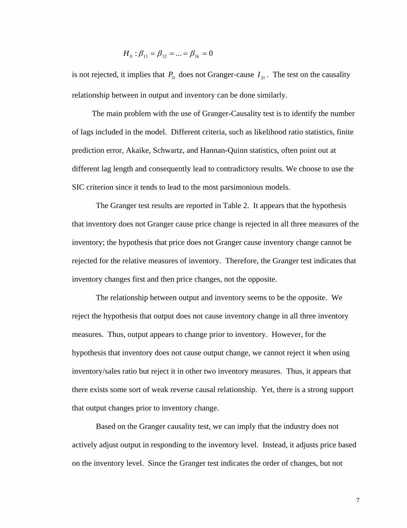
0...: 112110 ==== kH βββ

is not rejected, it implies that tP1 does not Granger-cause tI 2 . The test on the causality

relationship between in output and inventory can be done similarly.

The main problem with the use of Granger-Causality test is to identify the number

of lags included in the model. Different criteria, such as likelihood ratio statistics, finite

prediction error, Akaike, Schwartz, and Hannan-Quinn statistics, often point out at

different lag length and consequently lead to contradictory results. We choose to use the

SIC criterion since it tends to lead to the most parsimonious models.

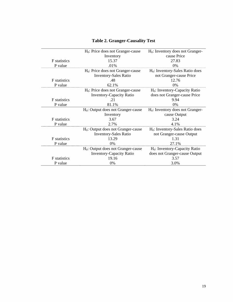
The Granger test results are reported in Table 2. It appears that the hypothesis

that inventory does not Granger cause price change is rejected in all three measures of the

inventory; the hypothesis that price does not Granger cause inventory change cannot be

rejected for the relative measures of inventory. Therefore, the Granger test indicates that

inventory changes first and then price changes, not the opposite.

The relationship between output and inventory seems to be the opposite. We

reject the hypothesis that output does not cause inventory change in all three inventory

measures. Thus, output appears to change prior to inventory. However, for the

hypothesis that inventory does not cause output change, we cannot reject it when using

inventory/sales ratio but reject it in other two inventory measures. Thus, it appears that

there exists some sort of weak reverse causal relationship. Yet, there is a strong support

that output changes prior to inventory change.

Based on the Granger causality test, we can imply that the industry does not

actively adjust output in responding to the inventory level. Instead, it adjusts price based

on the inventory level. Since the Granger test indicates the order of changes, but not

8

necessarily the cause of the change, we use regression analysis to investigate the

quantitative relationship between inventory, price and output.

5. PRICE ADJUSTMENTS

In order to investigate how price and output respond to inventory changes, we

conduct regression analyses based on a binary choice model. In particular, we estimate

the probability of price or output change due to inventory changes in the previous month.

We define a dichotomous variable, which equals 1 when the current price or output level

increases from the previous month and 0 otherwise. Additionally, in order to investigate

the delay of the responses to inventory changes, we include lagged value of inventory up

to four lags; i.e., the response to inventory changes happened up to four months before.1

We also add monthly dummy variables in the model to control for seasonal shocks.

Probit model has a number of advantages in studying binary choices and we

primarily use probit estimation in this study. Yet, it has some limitations especially in

dealing with auto-correlation of the error terms. Thus, we also use linear probability

model (LPM) in the estimation, which can address the problems of heteroskedasticity and

serial correlation (e.g., the Cochrane-Orcutt approach).

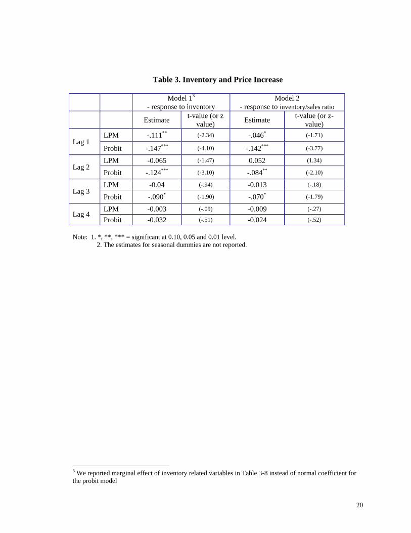
In Table 3, we report the estimated response of linerboard price increase to

previous months’ inventory changes. Inventory is measured by its level and its ratio to

total sales. In Table 4, inventory is measured by its ratio to the total capacity. In all

tables, the reported estimates based on Probit model are marginal effects (not the

estimated coefficients). Since the total production in the industry has been rising, the

1 We also run models with five or more lags, and they are statistically insignificant. In addition, we do not include more than one lags in the model due to the high degree of multicollinearity.

9

response of price or output should be more relevant to the changes in relative inventory,

not the actual level of inventory. Therefore, the model with inventory/sales and

inventory/capacity should serve as a better specification. For inventory/sales ratio,

however, one concern is that sales and prices may be simultaneously determined due to

the interaction of price and sales in the market. In this case, the ratio of inventory/sales

will be endogenous and cause problem in the estimation.2 To avoid this problem, the

ratio of inventory/capacity is used in the model. Given the long term nature of the

investment in the linerboard industry, the capacity is unlikely to be simultaneously

determined with current price change, and thus is unlikely to be endogenous. Therefore,

our discussion will be based on the results with inventory/capacity ratio.

Interestingly, as can be seen in Table 3 & 4, for different measures of inventory,

the results are not dramatically different. For example, in the LPM estimation, the

response of price hike is only statistically significant for one lag of the inventory (i.e. the

inventory in the previous month). In the Probit model, the response is statistically

significant for up to three lags. In all those cases, as expected, when inventory increases,

the probability for price hike will drop. In other words, if inventory declines, the price is

more likely to increase.

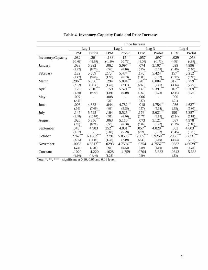
Based on the results in Table 4, if the ratio of inventory/capacity drops by 0.1 in

the current month, the probability of a price increase in the next month rises by 2%

according to the probit model and by 0.8% based on the LPM. For the same change of

the inventory/capacity ratio, the probability of price increase in the second month ahead

will rise 1.5%, and for the third month ahead will rise 1.0% (probit model). It appears

2 There might be a similar simultaneity issue between the current inventory and current price. We use previous inventory in our models. Since previous inventory is unlikely to be affected by the current price, the simultaneity problem should disappear.

10

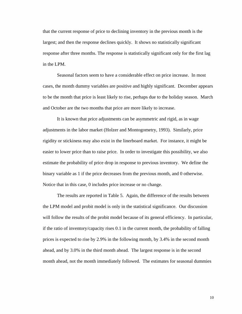
that the current response of price to declining inventory in the previous month is the

largest; and then the response declines quickly. It shows no statistically significant

response after three months. The response is statistically significant only for the first lag

in the LPM.

Seasonal factors seem to have a considerable effect on price increase. In most

cases, the month dummy variables are positive and highly significant. December appears

to be the month that price is least likely to rise, perhaps due to the holiday season. March

and October are the two months that price are more likely to increase.

It is known that price adjustments can be asymmetric and rigid, as in wage

adjustments in the labor market (Holzer and Montogometry, 1993). Similarly, price

rigidity or stickiness may also exist in the linerboard market. For instance, it might be

easier to lower price than to raise price. In order to investigate this possibility, we also

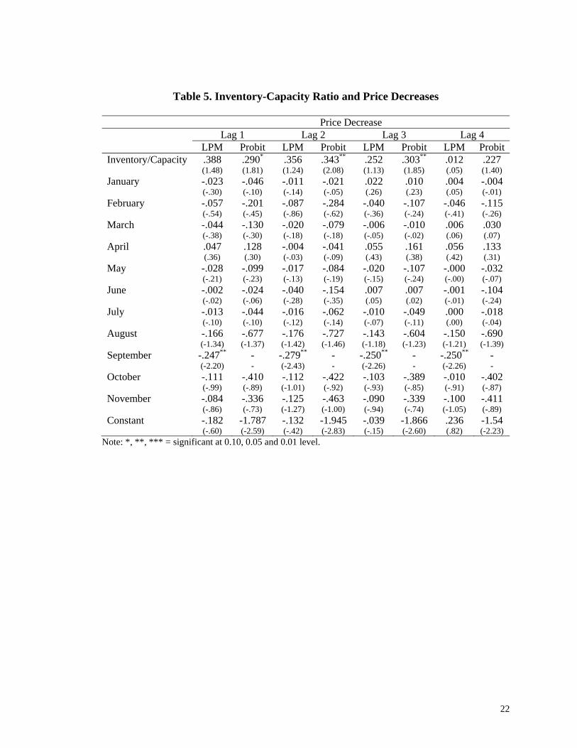
estimate the probability of price drop in response to previous inventory. We define the

binary variable as 1 if the price decreases from the previous month, and 0 otherwise.

Notice that in this case, 0 includes price increase or no change.

The results are reported in Table 5. Again, the difference of the results between

the LPM model and probit model is only in the statistical significance. Our discussion

will follow the results of the probit model because of its general efficiency. In particular,

if the ratio of inventory/capacity rises 0.1 in the current month, the probability of falling

prices is expected to rise by 2.9% in the following month, by 3.4% in the second month

ahead, and by 3.0% in the third month ahead. The largest response is in the second

month ahead, not the month immediately followed. The estimates for seasonal dummies

11

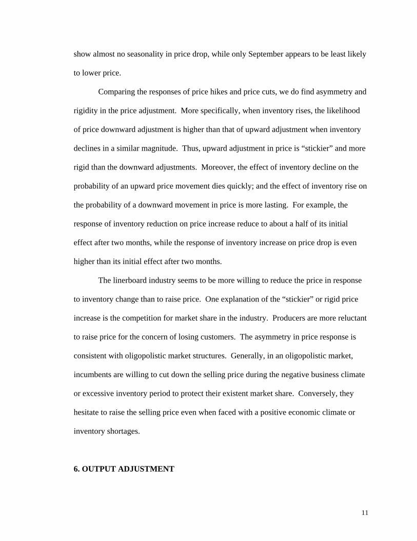
show almost no seasonality in price drop, while only September appears to be least likely

to lower price.

Comparing the responses of price hikes and price cuts, we do find asymmetry and

rigidity in the price adjustment. More specifically, when inventory rises, the likelihood

of price downward adjustment is higher than that of upward adjustment when inventory

declines in a similar magnitude. Thus, upward adjustment in price is “stickier” and more

rigid than the downward adjustments. Moreover, the effect of inventory decline on the

probability of an upward price movement dies quickly; and the effect of inventory rise on

the probability of a downward movement in price is more lasting. For example, the

response of inventory reduction on price increase reduce to about a half of its initial

effect after two months, while the response of inventory increase on price drop is even

higher than its initial effect after two months.

The linerboard industry seems to be more willing to reduce the price in response

to inventory change than to raise price. One explanation of the “stickier” or rigid price

increase is the competition for market share in the industry. Producers are more reluctant

to raise price for the concern of losing customers. The asymmetry in price response is

consistent with oligopolistic market structures. Generally, in an oligopolistic market,

incumbents are willing to cut down the selling price during the negative business climate

or excessive inventory period to protect their existent market share. Conversely, they

hesitate to raise the selling price even when faced with a positive economic climate or

inventory shortages.

6. OUTPUT ADJUSTMENT

12

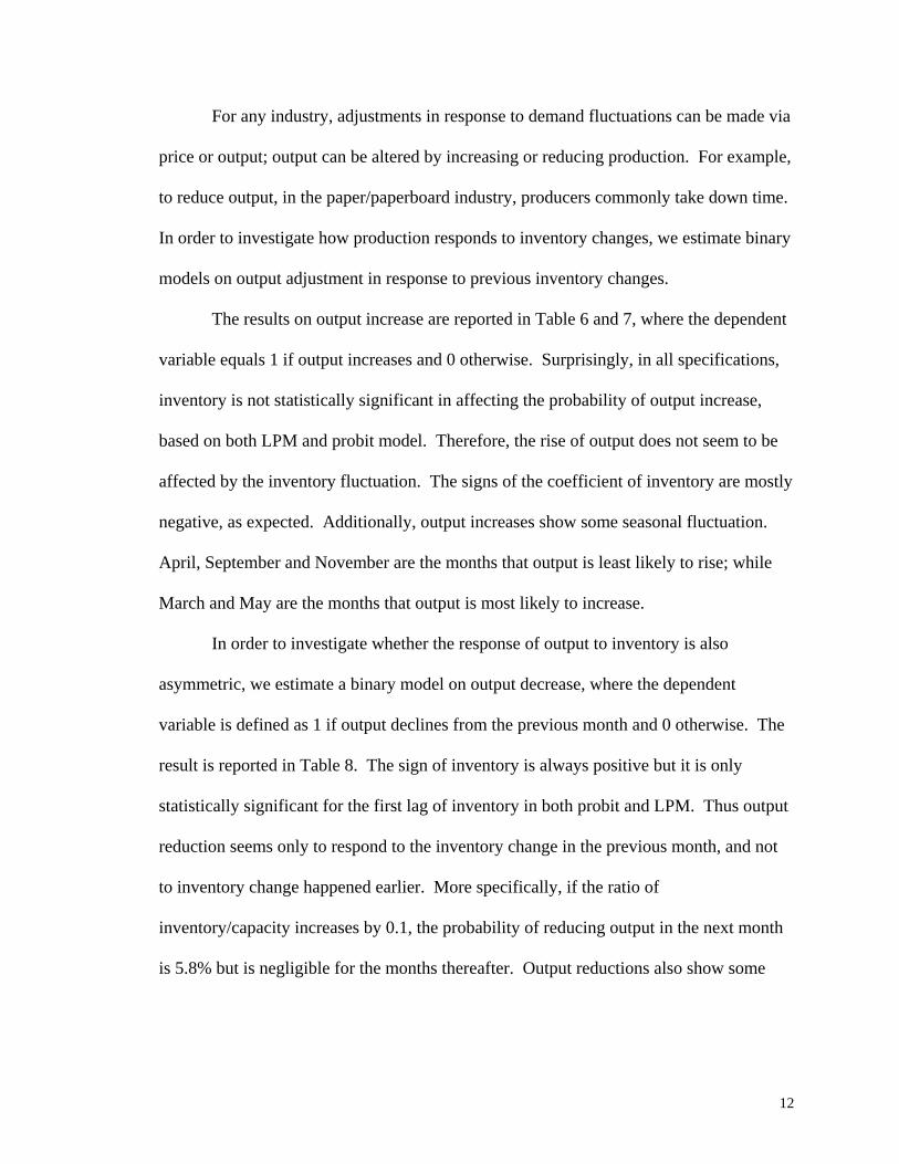
For any industry, adjustments in response to demand fluctuations can be made via

price or output; output can be altered by increasing or reducing production. For example,

to reduce output, in the paper/paperboard industry, producers commonly take down time.

In order to investigate how production responds to inventory changes, we estimate binary

models on output adjustment in response to previous inventory changes.

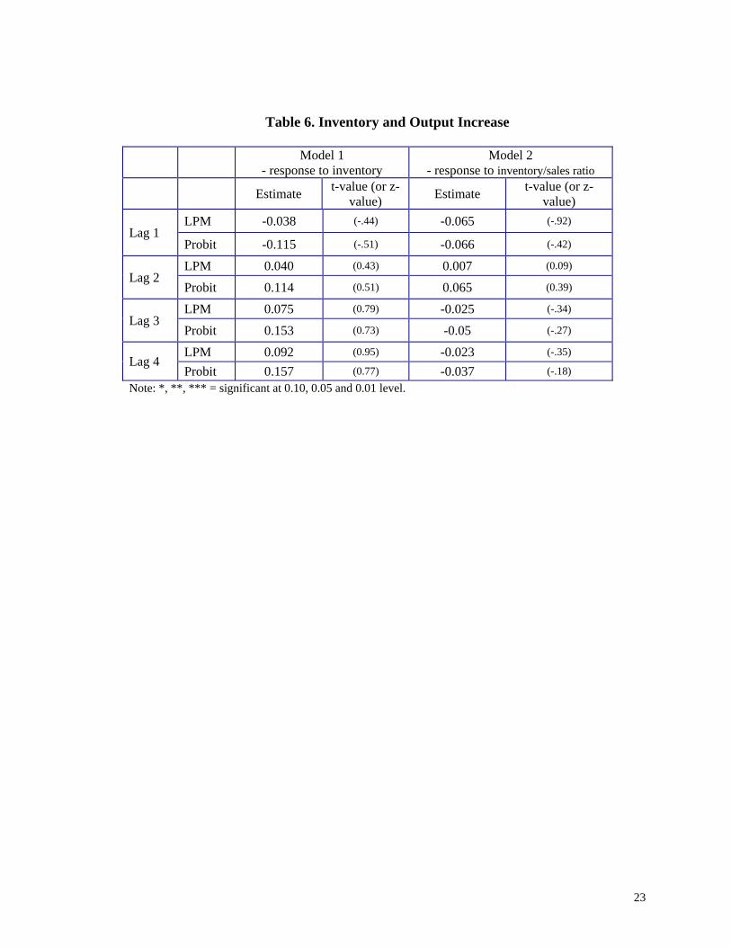
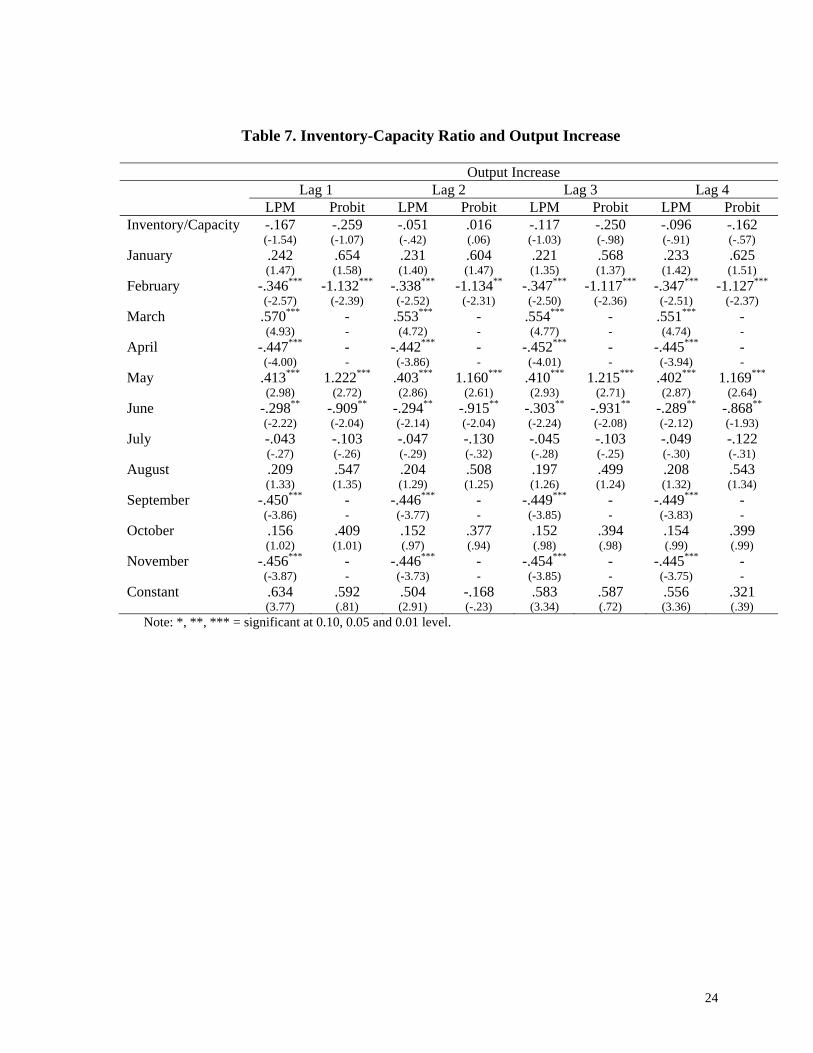
The results on output increase are reported in Table 6 and 7, where the dependent

variable equals 1 if output increases and 0 otherwise. Surprisingly, in all specifications,

inventory is not statistically significant in affecting the probability of output increase,

based on both LPM and probit model. Therefore, the rise of output does not seem to be

affected by the inventory fluctuation. The signs of the coefficient of inventory are mostly

negative, as expected. Additionally, output increases show some seasonal fluctuation.

April, September and November are the months that output is least likely to rise; while

March and May are the months that output is most likely to increase.

In order to investigate whether the response of output to inventory is also

asymmetric, we estimate a binary model on output decrease, where the dependent

variable is defined as 1 if output declines from the previous month and 0 otherwise. The

result is reported in Table 8. The sign of inventory is always positive but it is only

statistically significant for the first lag of inventory in both probit and LPM. Thus output

reduction seems only to respond to the inventory change in the previous month, and not

to inventory change happened earlier. More specifically, if the ratio of

inventory/capacity increases by 0.1, the probability of reducing output in the next month

is 5.8% but is negligible for the months thereafter. Output reductions also show some

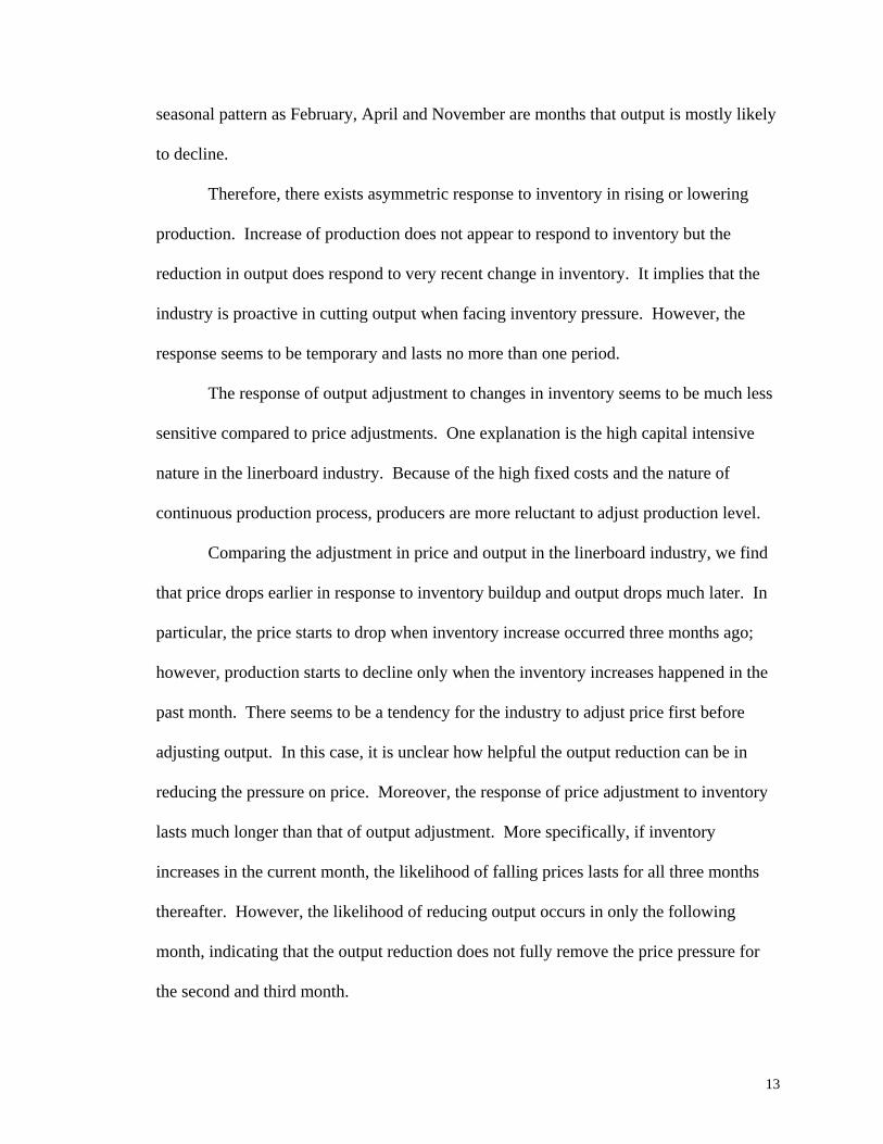
13

seasonal pattern as February, April and November are months that output is mostly likely

to decline.

Therefore, there exists asymmetric response to inventory in rising or lowering

production. Increase of production does not appear to respond to inventory but the

reduction in output does respond to very recent change in inventory. It implies that the

industry is proactive in cutting output when facing inventory pressure. However, the

response seems to be temporary and lasts no more than one period.

The response of output adjustment to changes in inventory seems to be much less

sensitive compared to price adjustments. One explanation is the high capital intensive

nature in the linerboard industry. Because of the high fixed costs and the nature of

continuous production process, producers are more reluctant to adjust production level.

Comparing the adjustment in price and output in the linerboard industry, we find

that price drops earlier in response to inventory buildup and output drops much later. In

particular, the price starts to drop when inventory increase occurred three months ago;

however, production starts to decline only when the inventory increases happened in the

past month. There seems to be a tendency for the industry to adjust price first before

adjusting output. In this case, it is unclear how helpful the output reduction can be in

reducing the pressure on price. Moreover, the response of price adjustment to inventory

lasts much longer than that of output adjustment. More specifically, if inventory

increases in the current month, the likelihood of falling prices lasts for all three months

thereafter. However, the likelihood of reducing output occurs in only the following

month, indicating that the output reduction does not fully remove the price pressure for

the second and third month.

14

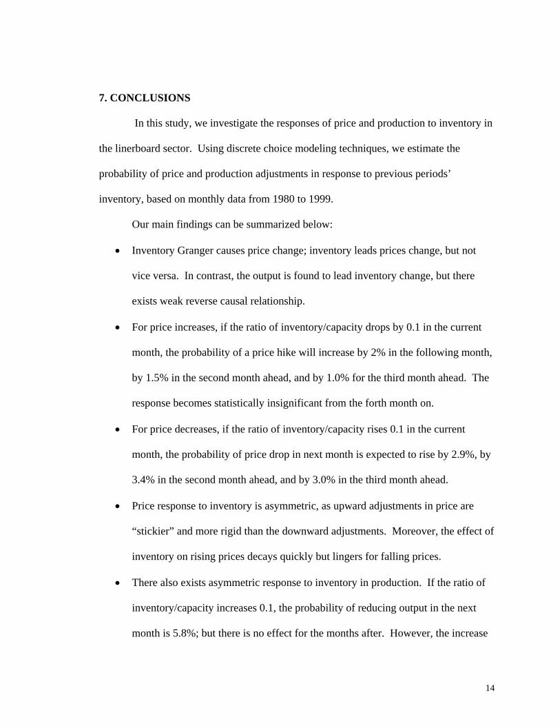
7. CONCLUSIONS

In this study, we investigate the responses of price and production to inventory in

the linerboard sector. Using discrete choice modeling techniques, we estimate the

probability of price and production adjustments in response to previous periods’

inventory, based on monthly data from 1980 to 1999.

Our main findings can be summarized below:

• Inventory Granger causes price change; inventory leads prices change, but not

vice versa. In contrast, the output is found to lead inventory change, but there

exists weak reverse causal relationship.

• For price increases, if the ratio of inventory/capacity drops by 0.1 in the current

month, the probability of a price hike will increase by 2% in the following month,

by 1.5% in the second month ahead, and by 1.0% for the third month ahead. The

response becomes statistically insignificant from the forth month on.

• For price decreases, if the ratio of inventory/capacity rises 0.1 in the current

month, the probability of price drop in next month is expected to rise by 2.9%, by

3.4% in the second month ahead, and by 3.0% in the third month ahead.

• Price response to inventory is asymmetric, as upward adjustments in price are

“stickier” and more rigid than the downward adjustments. Moreover, the effect of

inventory on rising prices decays quickly but lingers for falling prices.

• There also exists asymmetric response to inventory in production. If the ratio of

inventory/capacity increases 0.1, the probability of reducing output in the next

month is 5.8%; but there is no effect for the months after. However, the increase

15

of output does not seem to be affected by the inventory fluctuation. It appears

that the industry cuts output in response to inventory pressure, but the response

seems to be temporary and does not last for more than one period.

• Price falls last much longer in response to inventory buildup but output declines

end much sooner. There seems to be a tendency for the industry to adjust price

instead of adjusting output. The output adjustment seems to be short-lived and

does not help to remove the price pressure.

• There are some seasonal patterns in production and price dynamics. March and

October are the months that price is more likely to increase, but price cuts do not

show any clear seasonality. Output is most likely to increase March and May;

and is most likely to decline in February, April and November.

16

REFERENCES

Aguirregabiria, Victor. (1999) “The Dynamics of Markups and Inventories in Retailing

Firms.” Review of Economic Studies 66, 275-308.

Blinder, Alan S. (1983) “Inventories and Sticky Prices: More on the Microfoundations of

Macroeconomics.” American Economic Review 72, 334-48.

Booth, D.L., Kanetkar, V., Vertinsky, I., and Whistler, D. (1991) “An Empirical Model

of Capacity Expansion and Pricing Oligopoly with Barometric Price Leadership:

A Case Study of the Newsprint Industry in North America.” Journal of Industry

Economics 39, 255-76.

Buongiorno, J. and Lu, H.C. (1989) “Effects of Costs, Demand, and Labor Productivity

on the Prices of Forest Products in the United States, 1958-1984.” Forest Science

35, 349-63.

Christensen, Laurits Rolf and Caves, Richard E. (1997)“Cheap Talk and Investment

Rivalry in the Pulp and Paper Industry.” Journal of Industry Economics 45, 47-73.

Dagenais, Marcel G. (1976) “The Determination of Newsprint Prices.” Canadian Journal

of Economics 9, 442-61.

Granger, C. W. J. (1969). Investigating causal relations by econometric models and

cross-spectral methods. Econometrica, 37, 424–438.

Holzer, Harry J. and Montgomery, Edward B. (1993) “Asymmetries and Rigidities in

Wage Adjustments by Firms.” The Review of Economics and Statistics 75, 397-

408.

17

Li, Haizheng and Jifeng Luo (2005) “Industry Consolidation and Price: Evidence from

the U.S. Linerboard Industry,” Working Paper, School of Economics, Georgia

Tech.

Rich, S. U. (1983), “Pricing Leadership in the Paper Industry”, Industrial Marketing

Management, 12, 101-104.

18

Table 1. Descriptive Statistics

Variables Description Mean STDV Minimum Value

Maximum Value

Price U.S. linerboard price, in US$ per thousand short tons

347.48 63.08 250.00 530.00

Price Change

1 indicates U.S. linerboard price increase compared to previous period, 0 otherwise

0.12 0.33 0.00 1.00

Output U.S. linerboard output, in thousand short tons 1,606.50 309.01 925.00 2,224.00

Output Change

1 indicates U.S. linerboard output increase compared to previous period, 0 otherwise

0.53 0.50 0.00 1.00

Inventory U.S. linerboard inventory, in thousand short tons 1,895.59 209.09 1,305.40 2,336.60

Sales U.S. linerboard output excluding inventory, in thousand short tons

1,388.43 261.28 737.80 1,933.80

Inventory/ Sales Ratio

U.S. linerboard inventory divide U.S linerboard sales

1.41 0.27 0.92 2.73

Capacity U.S. linerboard capacity, in thousand tons 1,702.59 306.30 1,141.94 2,304.66

Inventory/ Capacity Ratio

U.S. linerboard inventory divide U.S linerboard capacity

1.14 0.17 0.79 1.69

19

Table 2. Granger-Causality Test

H0: Price does not Granger-cause Inventory

H0: Inventory does not Granger-cause Price

F statistics 15.37 27.83 P value .01% 0%

H0: Price does not Granger-cause Inventory-Sales Ratio

H0: Inventory-Sales Ratio does not Granger-cause Price

F statistics .48 12.76 P value 62.1% 0%

H0: Price does not Granger-cause Inventory-Capacity Ratio

H0: Inventory-Capacity Ratio does not Granger-cause Price

F statistics .21 9.94 P value 81.1% 0%

H0: Output does not Granger-cause Inventory

H0: Inventory does not Granger-cause Output

F statistics 3.67 3.24 P value 2.7% 4.1%

H0: Output does not Granger-cause Inventory-Sales Ratio

H0: Inventory-Sales Ratio does not Granger-cause Output

F statistics 13.29 1.31 P value 0% 27.1%

H0: Output does not Granger-cause Inventory-Capacity Ratio

H0: Inventory-Capacity Ratio does not Granger-cause Output

F statistics 19.16 3.57 P value 0% 3.0%

20

Table 3. Inventory and Price Increase

Model 13 - response to inventory

Model 2 - response to inventory/sales ratio

Estimate t-value (or z value) Estimate t-value (or z-

value)

Lag 1 LPM -.111** (-2.34) -.046* (-1.71)

Probit -.147*** (-4.10) -.142*** (-3.77)

Lag 2 LPM -0.065 (-1.47) 0.052 (1.34)

Probit -.124*** (-3.10) -.084** (-2.10)

Lag 3 LPM -0.04 (-.94) -0.013 (-.18)

Probit -.090* (-1.90) -.070* (-1.79)

Lag 4 LPM -0.003 (-.09) -0.009 (-.27)

Probit -0.032 (-.51) -0.024 (-.52) Note: 1. *, **, *** = significant at 0.10, 0.05 and 0.01 level. 2. The estimates for seasonal dummies are not reported.

3 We reported marginal effect of inventory related variables in Table 3-8 instead of normal coefficient for the probit model

21

Table 4. Inventory-Capacity Ratio and Price Increase

Price Increase Lag 1 Lag 2 Lag 3 Lag 4 LPM Probit LPM Probit LPM Probit LPM Probit Inventory/Capacity -.082* -.20*** -.138 -.15*** -.057 -.097* -.029 -.058

(-1.63) (-2.69) (-1.30) (-2.72) (-1.00) (-1.71) (-.53) (-.89) January .033 5.392*** .062 5.097*** .074 5.107*** .099 4.996***

(1.22) (8.75) (.54) (6.10) (.95) (6.59) (1.49) (5.95) February .129 5.609*** .275** 5.474*** .170* 5.424*** .157** 5.212***

(1.47) (9.66) (1.98) (6.33) (1.83) (6.82) (1.97) (5.95) March .296*** 6.356*** .294 5.894*** .320*** 6.004*** .317*** 5.759***

(2.52) (11.35) (1.40) (7.11) (2.69) (7.41) (3.14) (7.27) April .123 5.610*** .159 5.521*** .143* 5.391*** .167** 5.269***

(1.50) (9.70) (1.01) (6.10) (1.60) (6.78) (2.14) (6.23) May .007 - .008 - .006 - .000 -

(.42) - (.26) - (.37) - (.01) - June .006 4.882*** .044 4.782*** .018 4.754*** .036 4.637***

(.36) (7.09) (.81) (5.25) (.57) (5.64) (.85) (5.05) July .147 5.795*** .164 5.525*** .176* 5.621*** .190** 5.387***

(1.48) (10.07) (.91) (6.76) (1.77) (6.95) (2.24) (6.81) August .026 5.356*** .063 5.110*** .073 5.121*** .087 4.978***

(.76) (8.71) (.55) (6.00) (1.02) (6.42) (1.39) (5.86) September .045** 4.983 .252*** 4.831*** .057** 4.828*** .063 4.603***

(1.97) - (5.88) (5.29) (2.21) (5.52) (1.45) (5.25) October .2762*** 6.1582*** .2791 5.8505*** .2865*** 5.9250*** .2938*** 5.7231***

(2.35) (11.05) (1.33) (7.19) (2.49) (7.49) (3.03) (7.13) November .0053 4.8517*** .0293 4.7594*** .0254 4.7557*** .0382 4.6029***

(.25) (7.25) (.63) (5.32) (.59) (5.66) (.89) (5.23) Constant .1020 -4.220 .1628 -4.759 .0704 -5.382 .0343 -5.638 (1.60) (-4.40) (1.28) - (.99) - (.53) -

Note: *, **, *** = significant at 0.10, 0.05 and 0.01 level.

22

Table 5. Inventory-Capacity Ratio and Price Decreases

Price Decrease Lag 1 Lag 2 Lag 3 Lag 4 LPM Probit LPM Probit LPM Probit LPM ProbitInventory/Capacity .388 .290* .356 .343** .252 .303** .012 .227

(1.48) (1.81) (1.24) (2.08) (1.13) (1.85) (.05) (1.40) January -.023 -.046 -.011 -.021 .022 .010 .004 -.004

(-.30) (-.10) (-.14) (-.05) (.26) (.23) (.05) (-.01) February -.057 -.201 -.087 -.284 -.040 -.107 -.046 -.115

(-.54) (-.45) (-.86) (-.62) (-.36) (-.24) (-.41) (-.26) March -.044 -.130 -.020 -.079 -.006 -.010 .006 .030

(-.38) (-.30) (-.18) (-.18) (-.05) (-.02) (.06) (.07) April .047 .128 -.004 -.041 .055 .161 .056 .133

(.36) (.30) (-.03) (-.09) (.43) (.38) (.42) (.31) May -.028 -.099 -.017 -.084 -.020 -.107 -.000 -.032

(-.21) (-.23) (-.13) (-.19) (-.15) (-.24) (-.00) (-.07) June -.002 -.024 -.040 -.154 .007 .007 -.001 -.104

(-.02) (-.06) (-.28) (-.35) (.05) (.02) (-.01) (-.24) July -.013 -.044 -.016 -.062 -.010 -.049 .000 -.018

(-.10) (-.10) (-.12) (-.14) (-.07) (-.11) (.00) (-.04) August -.166 -.677 -.176 -.727 -.143 -.604 -.150 -.690

(-1.34) (-1.37) (-1.42) (-1.46) (-1.18) (-1.23) (-1.21) (-1.39) September -.247** - -.279** - -.250** - -.250** -

(-2.20) - (-2.43) - (-2.26) - (-2.26) - October -.111 -.410 -.112 -.422 -.103 -.389 -.010 -.402

(-.99) (-.89) (-1.01) (-.92) (-.93) (-.85) (-.91) (-.87) November -.084 -.336 -.125 -.463 -.090 -.339 -.100 -.411

(-.86) (-.73) (-1.27) (-1.00) (-.94) (-.74) (-1.05) (-.89) Constant -.182 -1.787 -.132 -1.945 -.039 -1.866 .236 -1.54 (-.60) (-2.59) (-.42) (-2.83) (-.15) (-2.60) (.82) (-2.23)

Note: *, **, *** = significant at 0.10, 0.05 and 0.01 level.

23

Table 6. Inventory and Output Increase

Model 1 - response to inventory

Model 2 - response to inventory/sales ratio

Estimate t-value (or z-value) Estimate t-value (or z-

value)

Lag 1 LPM -0.038 (-.44) -0.065 (-.92)

Probit -0.115 (-.51) -0.066 (-.42)

Lag 2 LPM 0.040 (0.43) 0.007 (0.09)

Probit 0.114 (0.51) 0.065 (0.39)

Lag 3 LPM 0.075 (0.79) -0.025 (-.34)

Probit 0.153 (0.73) -0.05 (-.27)

Lag 4 LPM 0.092 (0.95) -0.023 (-.35)

Probit 0.157 (0.77) -0.037 (-.18) Note: *, **, *** = significant at 0.10, 0.05 and 0.01 level.

24

Table 7. Inventory-Capacity Ratio and Output Increase

Output Increase Lag 1 Lag 2 Lag 3 Lag 4 LPM Probit LPM Probit LPM Probit LPM Probit Inventory/Capacity -.167 -.259 -.051 .016 -.117 -.250 -.096 -.162

(-1.54) (-1.07) (-.42) (.06) (-1.03) (-.98) (-.91) (-.57) January .242 .654 .231 .604 .221 .568 .233 .625

(1.47) (1.58) (1.40) (1.47) (1.35) (1.37) (1.42) (1.51) February -.346*** -1.132*** -.338*** -1.134** -.347*** -1.117*** -.347*** -1.127***

(-2.57) (-2.39) (-2.52) (-2.31) (-2.50) (-2.36) (-2.51) (-2.37) March .570*** - .553*** - .554*** - .551*** -

(4.93) - (4.72) - (4.77) - (4.74) - April -.447*** - -.442*** - -.452*** - -.445*** -

(-4.00) - (-3.86) - (-4.01) - (-3.94) - May .413*** 1.222*** .403*** 1.160*** .410*** 1.215*** .402*** 1.169***

(2.98) (2.72) (2.86) (2.61) (2.93) (2.71) (2.87) (2.64) June -.298** -.909** -.294** -.915** -.303** -.931** -.289** -.868**

(-2.22) (-2.04) (-2.14) (-2.04) (-2.24) (-2.08) (-2.12) (-1.93) July -.043 -.103 -.047 -.130 -.045 -.103 -.049 -.122

(-.27) (-.26) (-.29) (-.32) (-.28) (-.25) (-.30) (-.31) August .209 .547 .204 .508 .197 .499 .208 .543

(1.33) (1.35) (1.29) (1.25) (1.26) (1.24) (1.32) (1.34) September -.450*** - -.446*** - -.449*** - -.449*** -

(-3.86) - (-3.77) - (-3.85) - (-3.83) - October .156 .409 .152 .377 .152 .394 .154 .399

(1.02) (1.01) (.97) (.94) (.98) (.98) (.99) (.99) November -.456*** - -.446*** - -.454*** - -.445*** -

(-3.87) - (-3.73) - (-3.85) - (-3.75) - Constant .634 .592 .504 -.168 .583 .587 .556 .321 (3.77) (.81) (2.91) (-.23) (3.34) (.72) (3.36) (.39)

Note: *, **, *** = significant at 0.10, 0.05 and 0.01 level.

25

Table 8. Inventory Capacity Ratio and Output Decrease

Output Decrease Lag 1 Lag 2 Lag 3 Lag 4 LPM Probit LPM Probit LPM Probit LPM Probit Inventory/Capacity .321*** .578** .172 .249 .153 .275 .078 .108

(2.65) (2.24) (1.18) (1.05) (1.15) (1.06) (.60) (.43) January -.320*** -1.375*** -.305*** -1.257** -.287*** -1.180** -.301*** -1.242**

(-2.62) (-2.40) (-2.48) (-2.25) (-2.40) (-2.10) (-2.43) (-2.23) February .494*** 1.412*** .473*** 1.310*** .496*** 1.404*** .494*** 1.395***

(3.71) (3.13) (3.41) (2.89) (3.59) (3.11) (3.56) (3.09) March -.388*** - -.360*** - -.356*** - -.351*** -

(-3.66) - (-3.33) - (-3.31) - (-3.24) - April .546*** 1.719*** .523*** 1.595*** .552*** 1.707*** .539*** 1.628***

(4.47) (3.48) (3.96) (3.27) (4.42) (3.51) (4.08) (3.36) May -.375*** - -.359*** - -.363*** - -.351*** -

(-3.59) - (-3.34) - (-3.35) - (-3.24) - June -.004 -.006 -.020 -.070 .003 .024 -.009 -.030

(-.03) (-.01) (-.13) (-.17) (.02) (.06) (-.06) (-.07) July -.063 -.211 -.059 -.173 -.057 -.169 -.051 -.141

(-.45) (-.49) (-.40) (-.41) (-.38) (-.40) (-.34) (-.34) August -.166 -.514 -.164 -.496 -.147 -.426 -.156 -.472

(-1.20) (-1.17) (-1.15) (-1.14) (-1.05) (-.98) (-1.08) (-1.09) September .400*** 1.086*** .385*** 1.010*** .399*** 1.063*** .399*** 1.057***

(2.80) (2.55) (2.61) (2.39) (2.73) (2.52) (2.71) (2.52) October -.311*** -1.316*** -.307*** -1.279** -.302*** -1.266** -.303*** -1.266**

(-2.70) (-2.34) (-2.58) (-2.30) (-2.57) (-2.27) (-2.52) (-2.29) November .462*** 1.314*** .437*** 1.191*** .455*** 1.261*** .446*** 1.215*** (3.27) (2.99) (3.03) (2.75) (3.20) (2.91) (3.09) (2.82) Constant -.004 -2.032 .166 -1.068 .176 -1.194 .263 -.693 (-.03) (-2.55) (.94) (-1.50) (1.04) (-1.46) (1.60) (-.90)

Note: *, **, *** = significant at 0.10, 0.05 and 0.01 level.

26

Figure 1. The U.S. linerboard price and inventory pattern, 1980-1999

2 0 0

2 5 0

3 0 0

3 5 0

4 0 0

4 5 0

5 0 0

5 5 0

1 2 0 0

1 4 0 0

1 6 0 0

1 8 0 0

2 0 0 0

2 2 0 0

2 4 0 0

2 6 0 0

8 0 8 2 8 4 8 6 8 8 9 0 9 2 9 4 9 6 9 8

I N V E N T O R Y P R I C E

Figure 2. The U.S. linerboard capacity and sales pattern, 1980-1999

6 0 0

8 0 0

1 0 0 0

1 2 0 0

1 4 0 0

1 6 0 0

1 8 0 0

2 0 0 0

1 0 0 0

1 2 0 0

1 4 0 0

1 6 0 0

1 8 0 0

2 0 0 0

2 2 0 0

2 4 0 0

8 0 8 2 8 4 8 6 8 8 9 0 9 2 9 4 9 6 9 8

C A P A C I T Y S A L E S

27

Figure 3. The U.S. linerboard relative inventory pattern, 1980-1999

Note: insa=inventory/sales, inca=inventory/capacity

0.8

1.2

1.6

2.0

2.4

2.8

80 82 84 86 88 90 92 94 96 98

insa inca