Embed Size (px)
Citation preview

A Dynamic Model of Price Discrimination and InventoryManagement at the Fulton Fish Market∗
Kathryn GraddyBrandeis University†
George HallBrandeis University‡
August 2010
Abstract
We estimate a dynamic profit-maximization model of a fish wholesaler who can observe consumercharacteristics, set individual prices, and thus engage in third-degree price discrimination. Simu-lated prices and quantities from the model exhibit the key features observed in a set of high qualitytransaction-level data on fish sales collected at the Fulton Fish Market. The model’s predictions arethen compared to the case in which the wholesaler must post a single price to all retailers. We find theadded revenue the wholesaler receives from price discriminating to be small.
Keywords: fish, price discrimination, yield management, dynamic programming, indirect inferenceJEL classification: L1, D4, D21, L81, C15
∗We thank Jonathan Hamilton, two anonymous referees, and participants at the Brandeis IBS brown-bag seminar for helpfulcomments.
†Department of Economics, Brandeis University, 415 South Street, Waltham, MA 02454-9110; phone: (781) 736-8616;e-mail: [email protected]
‡Department of Economics, Brandeis University, 415 South Street, Waltham, MA 02454-9110; phone: (781) 736-2242;e-mail: [email protected]

1 Introduction
What are the benefits to a wholesaler of price discrimination resulting from privately negotiated prices
versus posting a single price? At first glance, one might expect a fish wholesale market to be highly
competitive. However, the Fulton Fish market, with its storied history of mafia involvement, has substantial
barriers to entry. These barriers to entry have caused an imperfectly competitive environment characterized
by negotiated prices. Our aim in this paper is to measure the magnitude of the increase in profits resulting
from price discrimination versus posting a single price.
We solve and estimate a dynamic profit-maximization model of a fish wholesaler. Stocks of fish arrive
every morning, and the fish must be sold within a relatively short period of time. Throughout the day,
retailers arrive sequentially and randomly, but when a retailer shows up, the wholesaler observes his type
and thus knows his price elasticity. Therefore the wholesaler can price discriminate across different types
of retailers. The fish wholesaler is solving two problems simultaneously: 1) how to optimally price his
stock of fish which is falling in value over time and is replenished only once a day; and 2) how to optimally
price discriminate across customers with differing price elasticities.
Our model is able to successfully match several key features of the Fulton Fish Market. In particular
the model predicts, as we see in the data, that Asian retailers pay about 5 cents per pound less for fish than
white retailers. More generally the model matches the mean and variance of prices with large differences
in prices across different days as well as considerable intra-day price volatility. Overall, we conclude that
the model is a reasonable approximation of the behavior of a Fulton Fish Market wholesaler.
We then impose the restriction that the fish wholesaler must post a uniform price to all retailers, and
is therefore unable to price discriminate. In this case, white retailers with inelastic demand pay lower
prices and purchase larger quantities of fish. The more price-elastic Asian retailers pay higher prices and
purchase less fish. From both types, the wholesaler earns less revenue. However the magnitudes are small.
We find that posting a single price only generates about $6 per day less revenue (about 15/100 of one
percent of total revenue) compared to price discriminating.
While our model is intended to provide an accurate representation of the behavior of a particular fish
wholesaler, the problem of determining the optimal price of a stock of depreciating assets is a classic
problem in economics and operations research. In operations research the study of dynamically pricing
an inventory stock falls under the headings revenue management or yield management.1 In the economics
1This literature which started with Whiten (1955) and Karlin and Carr (1962) is reviewed by Federgruen and Heching (1999)and Elmaghraby and Keskinocak (2003).
2
literature, work by Reagan (1982), Aguirregabiria (1999), Zettelmeyer, Scott Morton and Silva-Risso
(2003), Chan, Hall, and Rust (2004), Sweeting (2008), and Copeland, Dunn, and Hall (2010) study the
interaction between inventory management and pricing. Our model differs from these others in that the
timing of new procurements of inventories is fixed though the quantity is stochastic. While these other
papers focus on durable goods, such as automobiles and steel, or goods that expire at a pre-determined date,
such as baseball tickets, hotel rooms and airline seats, our paper focuses on fish – a good that depreciates
steadily but quickly.
This paper proceeds as follows. In the next section we discuss the importance of price discrimination
and previous papers that have highlighted discriminatory settings. In section 3, we discuss the details
of the Fulton Fish Market, the market on which our structural model is based. In section 4 we develop
our model, and in section 5, we present our estimation strategy. We report our findings in section 6 and
conclude our analysis in section 7.
2 Price Discrimination versus a Single Posted Price
In an early empirical paper on price discrimination, Borenstein (1991) demonstrated price discrimination in
the retail gasoline market, a market that at first glance appeared to be more competitive than monopolistic
(and in this way similar to the Fulton Fish Market) by estimating price-cost margins. More recent work
has focused on conducting welfare analyses of price discrimination by using structural models. Hastings
(2009) focuses on the wholesale gasoline market, Villas-Boas (2009) focuses on the German coffee market,
and Langer (2009) focuses on price discrimination in new vehicle sales. In each of these papers, the
authors estimate a model of supply and demand with price discrimination and then use these estimates to
investigate a counterfactual scenario with a single posted price. A primary purpose of their analyses is to
compare total welfare under various scenarios.
Our paper is similar to the above papers in that it estimates a model of supply and demand with price
discrimination and then investigates a counterfactual scenario with a single posted price. However, our
paper differs in that its focus is the advantage to the dealer of price discrimination versus posted prices.
Both in purpose and in methodology, our paper is closest to Chan, Hall and Rust (2004), in which the
authors compare the case of price discrimination in the steel market by a wholesaler to the case of uniform
pricing by estimating a dynamic model of price discrimination and inventory adjustment.
Everything else equal, if a firm has the ability to price discriminate, then the firm can raise its rev-
3

enue by doing so. However, everything else is very rarely equal. Price discrimination, by its nature,
incurs a number of costs that are difficult to measure. As Rust and Hall (2003) argue, posting a fixed
price eliminates the need for consumers to engage in costly search and thus may increase demand from
consumers with high search costs. Secondly, price discrimination that results from bargaining incurs ne-
gotiation costs. As pointed out by Wang (1995), bargaining versus posting a price requires the seller to
hire additional employees to mingle with buyers; posting a price is simpler and cheaper, but does not allow
discrimination. Finally, price discrimination can result in psychological costs to buyers that over the long
term can be harmful to sellers. These costs are similar to the constraints on profit seeking resulting from
fairness concerns as pointed out by Kahneman, Knetsch and Thaler (1986).
These transaction costs, most of which are very difficult to measure directly, are necessarily bounded
by the marginal profits – with everything else held equal – that a seller receives from price discrimina-
tion. By using a structural analysis, we bound these costs by estimating the marginal profits from price
discrimination relative to a single price strategy under a counterfactual scenario holding everything else
equal.
3 The Fulton Fish Market
In this section, we provide details of the Fulton Fish Market. Through a contact at the Fulton Fish Market
in New York City, one of the authors, Kathryn Graddy, collected a detailed set of transaction level data for
a single fish wholesaler for 22 weeks from December 2, 1991 to May 8, 1992 (111 business days and 2,868
transactions) for one type of fish: whiting. For each transaction, she collected the order the transaction
occurred, the price paid, the quantity sold, the quality of the fish, and several characteristics of the retailer
(e.g. ethnicity, location and type of retail outlet). The appendix provides a summary of the number of
transactions on which Graddy observed ethnicity and time of transaction.2
For each day in the sample, Graddy also collected the quantity of whiting received by this wholesaler
and the weather. These data have been described and extensively analyzed in Graddy (1995), Angrist,
Graddy, and Imbens (2000), Graddy (2006), Lee (2007), and Graddy and Kennedy (2010). Given that
these data are high quality and that the fish wholesaler’s problem is relativity straight forward and well
understood, we wish to formulate a structural model that can replicate the main features of these data. We
2Kathryn Graddy spent four weeks hand-collecting data at the market. Ethnicity was not observed for all transactions as theethnicity could only be identified for retailers with transactions that occurred during the time Graddy spent at the market. Forthe week Graddy was not at the market, time of transaction was only observed on cash transactions. For less than one percent ofthese transactions (23 out of a total of 2868) price was not recorded.
4

have attempted to make our model an accurate representation of a Fulton Fish Market wholesaler focusing
on the following details of this market.
At the time the data were collected in the early 1990s, the market was open for business from 3:00
to 9:00 in the morning on Monday and Thursday and from 4:00 to 9:00 on Tuesday, Wednesday, and
Friday. There were 60 registered wholesalers in the market, but only 35 wholesalers actively operating in
the market. Not all wholesalers carried all types of fish. Only six major wholesalers sold whiting.3
The whiting was supplied by fishermen’s cooperatives, packing houses, and smaller fishing boats in
New Jersey, Long Island, and Connecticut each day before the market opens. The price the wholesaler
paid a supplier for a particular day’s supply of whiting was determined at the end of the day by the prices
the wholesaler received for the whiting on that particular day. Each supplier serviced multiple wholesalers.
A supplier would refuse to deliver fish to a wholesaler from whom he continually received a poor price
relative to other wholesalers. In this way, wholesalers competed with each other for fish supplied in the
future by the amount they paid the suppliers for fish on a particular day. The wholesaler stated that he kept
5-15 cents on each pound of whiting sold (although this margin could not be independently verified).
A wholesaler often had a good idea of the quantity that would be available before the market’s close on
the previous day. Quantity supplied was primarily determined by weather conditions with wind and waves
being the most important determinant of the quantity of fish caught. Days were classified as stormy when
wave heights were greater than 4.5 feet and wind speed is greater than 18 knots. Wind speed and wave
height are moving averages of the last three days’ wind speed and wave height before the trading day, as
measured off the coast of Long Island and reported in the New York Times boating forecast. Quantities fall
and prices rise when there are storms, and quantities rise and prices fall in good weather. Holding day of
the week constant, the average quantity sold on a clear day was 2,371 pounds more than on a stormy day.
Conversely, the average price was 32 cents less per pound than on a clear day.
The quantity of whiting delivered for a particular day was received in its entirety before the market
opened. If one wholesaler did not receive what he perceived to be enough whiting, another wholesaler
would sell him whiting before the market opened. The price was set not at the time of sale, but was
determined toward the end of the trading day.
Anyone could purchase fish at the Fulton Fish Market, but small quantities were not sold. For whiting,
the minimum quantity sold was one box, approximately 60 pounds (except as favors to regular retailers).
3Data on whiting were collected for three reasons. More transactions take place in whiting than in any other fish. Whitingdoes not vary substantially in size and quality. Finally, and perhaps most importantly, the wholesaler from whom the data werecollected suggested that the whiting salesman would be the only salesman amenable to having an observer.
5
Most of the retailers were repeat buyers, but retailer-wholesaler relationships varied. Some retailers regu-
larly purchased from one wholesaler, and other retailers purchased from various wholesaler. Most retailers
followed distinct purchasing patterns. Monday, Thursday and Friday were big days, while Tuesday and
Wednesday were relatively quiet. Whiting stayed sufficiently fresh to sell for at most four days after it was
received. However, it was usually sold either the day that it was received or the day after. About half of
the time, the total quantity received exceeded total sales.
As would be expected, there was a small amount of oversupply as some inventory loss is inevitable in
the selling process, especially given the perishable nature of fish. Over 111 days in late 1991 and early
1992, the total quantity received is 713,365 pounds, and the total quantity sold is 702,128 (as noted in the
total on the inventory sheets by the wholesaler). Using the inventory sheet total sold, the total quantity
received minus the total quantity sold differs a total of by 11,237 pounds, which amounts to about 1.6
percent of total sales, or approximately 101 pounds per day. A total of 23 transactions or 9,187 pounds do
not specify a price, and of this, for 14 transactions (for a total of 5652 pounds), the customer is listed as
“dumped”. 4
The Fulton Fish Market had no posted prices and each wholesaler was free to charge a different price
to each retailer. If a retailer wished to buy a particular quantity of fish, he would ask a wholesaler for the
price. The wholesaler would quote a price and the retailer would usually either buy the fish or walk away.
Prices were generally quoted in five-cent increments. Wholesalers were discreet when naming a price. A
particular price was for a particular retailer.
Crime and the mafia have had a long history at the Fulton Fish Market. Law enforcement experts point
out the mafia can find it easier to gain a foothold when a relatively small number of people and businesses
operate in a single location. At one point in the early 1900s, oystermen and fishermen refused to enter
the harbor without police guard (Slanetz, 1986). Since then, there were continued reports of extortion,
“tapping” - that is, stealing fish, income tax evasion and obtaining false loans. All transporting of fish at the
market was done by the loading teams, a system which evolved over 75 years ago (Raab, 1996), and these
loading companies formed a monopoly over the loading and unloading of fish. Loading companies also
controlled parking in city streets adjacent to the market, partially through extortionate measures (Raab,
1995). Effectively, one could not park on city parking spaces near the market without paying. While
4If the individual transactions are summed, the total sold is 703,148. The total sum of the transactions minus the total quantitysold differs by a total of 10,217 pounds, or approximately 929 pounds per day. The transactions without a price do not explainthe discrepancy – it is not clear why the total number on the inventory sheet differs slightly from the total number of transactions.However, this discrepancy is small.
6

Figure 1: Day-to-Day Prices for Whiting (in $ per pound)
headlines such as “Mafia Runs Fulton Fish Market, U.S. Says in Suit to Take Control,” (Lubasch, 1987)
may be overblown, the continuing presence of the mafia in the loading and market operations during the
time of data collection certainly represented barriers to entry. These barriers to entry were undoubtedly a
factor in allowing the continuation of imperfect competition at the market.
Prices varied tremendously. For example, the average price in a whiting transaction on Friday, May 1,
1992, was $.33/lb., and the average price on Friday, May 8, was $1.75/lb., an increase of almost six-fold.
Figure 1 is a high-low price chart, where the bottom of the vertical line shows the low price for that day
and the top of the vertical line shows the high price for that day. The high intraday volatility was primarily
due to changes in price throughout the day, but some of the volatility could be attributed to differences in
qualities of fish. There was often a large decline in price after 7:00 a.m, but the pattern before 7:00 a.m. is
not easily predictable. There was a higher intraday volatility on Friday than on other days.
Figure 2 indicates total daily sales, which varied considerably. Daily supply shocks, primarily caused
by weather, were largely responsible for the high volatility in day-to-day prices. The simple correlation
7

Figure 2: Day-to-Day Volumes of Whiting (in pounds)
between total daily sales and average daily price is -.32.
Graddy observed that wholesalers were quoting lower prices to Asian retailers for the same box of fish.
The price difference would usually be about 5 cents, though it could go to as large as 10 cents. Regressions
that carefully control for other variables, including time of sale and quality, indicated that whites pay on
average 6.3 cents per pound more on each transaction for the same type and quality of fish than do Asian
retailers (Column 1 in Table 2 of Graddy, 1995). While quality controls could naturally be imperfect, these
regressions were consistent with observations.
These price differences were able to persist due to the different characteristics of the retailers. There
was strong anecdotal evidence that Asian retailers were more elastic than white retailers. Asians retailers
would resell their whiting as whole fish in retail shops, fish sandwiches in fry shops, and would make them
into fish balls. Most of these establishments were located in very poor neighborhoods. Retailers had little
scope to raise the price of whiting for their ultimate consumers. Consequently, they would bargain very
hard at the market.
8

In contrast, many white retailers (though not all) had more scope to pass on prices to consumers. For
example, for the local fish retailer in Princeton, New Jersey, whiting was a very small part of his purchase;
he would spend no time shopping around for price on whiting. If prices were especially high at the market,
he could explain to his consumers that fish were expensive at Fulton Street and his consumers would often
be willing to absorb costs by paying higher prices. Finally since prices were quoted discretely and white
retailers rarely socialized with Asian retailers it is unlikely that either white retailers or Asian retailers
knew that each group was being charged different prices.
Although Asians on average purchased larger quantities, there is little reason to suspect that quan-
tity differences are driving the price discrimination. There are no large fixed costs to consummating a
transaction. Transportation is always provided by the whiting retailer. One salesman is employed for
whiting regardless of the number of retailers, so time spent negotiating does not appear to be a factor. Fur-
thermore, in reduced form price regressions reported in Table 2 of Graddy (1995) customers with higher
average quantities purchased per transaction did not receive significantly lower prices. As we model be-
low, wholesalers are concerned with unsold inventory, which effects their pricing decisions. We discuss
this further in the interpretation section below.
Given the small number of wholesalers (six at the time) who carried whiting and the long tenure
of many of the wholesalers, the structure of the Fulton Fish Market for whiting, at least in the early
1990s, appeared conducive to tacit collusion, rather than perfect competition. Wholesalers traded with
each other before the market opened. They would price fish on a daily and sometimes hourly basis and
would receive feedback from the retailers on other wholesalers’ prices. Wholesalers in such a situation
could easily become very good at tacit communication. Moreover, entry into this market was limited
because suppliers provided the whiting on credit to established wholesalers - and it is not clear they would
be willing to provide fish on credit to a new entrant. The presence of organized crime in the market may
also have discouraged entry. Hence there is little reason to expect the marginal profits earned from price
discrimination to be competed away.
4 The Model
In this section we present our dynamic, profit maximization model of a fish wholesaler. The model is
designed to be consistent with the structure of the Fulton Fish Market and to capture the basic features of
the price and quantity data presented above. In this spirit, there are shocks to both supply and demand.
9

The daily supply of fish is stochastic and depends on the weather with storms reducing the average size of
the catch. On the demand side, the arrival of retailers each day is uncertain and their individual demand
curves vary as well. Fish can be stored but depreciates quickly. As retailers arrive sequentially, the fish
wholesaler chooses a price for each individual retailer. If he sets too high a price, he risks having fish go
bad; if he sets too low a price, he foregoes the potential to sell the fish to subsequent retailers at a higher
price. The wholesaler can price discriminate since he observes each retailer’s type before quoting a price.
The optimal pricing strategy is determined by recursively solving his dynamic optimization problem.
Formally, our fictional fish wholesaler is open for business five days a week, Monday through Friday,
for five hours each day. At the start of each workday, he receives a catch, C, which varies by the day
of the week and the weather. The weather can be in one of two states, calm or stormy, and follows a
Markov chain. The day’s catch is drawn from a truncated log-normal distribution with a mean µc(d,w)
and a standard deviation σc(d,w) with d = 1,2, ...,5 denoting the day of the week (Monday-Friday) and w
denoting the day’s weather, as being either calm or stormy.
Each five-hour workday is divided into 60 five minute periods indexed by t. At the start of each period
t, the fish wholesaler holds inventory It . Retailers arrive sequentially. There are two types of retailers,
Asians and whites, indexed by n, who arrive with probability λn, with
λ0 +λasian +λwhite = 1 (1)
where λ0 is the probability that no retailer shows up. Only a single retailer may show up during a given
period. In period t, if a retailer arrives, the fish wholesaler observes the retailer’s type. He knows each
retailer of type n has a stochastic constant elasticity demand curve for fish,
log(qt) = µnq +α(d)− γn log(pt)+ εn
t (2)
where εnt is distributed i.i.d N(0,σεn). As in Graddy (1995) and Angrist, Graddy and Imbens (2000), we
do not allow for cross-price elasticities. Whiting is a good deal cheaper than any other fish, and within
the observed range of prices, there did not exist good substitutes. The term α(d) allows the constant term
to vary by day of the week but stays fixed with the different types of retailers. We normalize α(5) (i.e.
Friday) to zero. Sales, qt , are constrained to
60≤ qt ≤ It , (3)
where It is the stock of fish available for sale at the start of period t. This constraint rules out back-orders
and implements the observed minimum purchase size of 60 pounds (one box). If at the quoted price, the
10

retailer demands fewer than 60 pounds, no sale occurs. Thus the one-box minimum pins down the retailer’s
reservation price above which he will walk away. If the retailer demands more than the current level of
inventory, we set qt = It , and the wholesaler is stocked out until the following morning.
Fish depreciates at a constant rate throughout the day, so the evolution of the wholesaler’s stock fol-
lows:
It+1 = (1− δ)It −qt for t = 1,2, ...,59 (4)
where δ is the intra-day depreciation rate. Between weekdays, the wholesaler’s stock is augmented by the
catch, so the law of motion becomes
I1 = (1− δ)I60−q60 +C(d′,w′) for d′ = 2,3,4,5 (5)
with δ denoting the overnight depreciation rate and the subscript 60 denoting the last (i.e. the 60th) trading
period of the day. Over the weekend, this law of motion becomes
I1 = (1− δ)I60−q60 +C(1,w′) (6)
with δ denoting the over-the-weekend depreciation rate.
Since we do not observe directly how revenue is split between the wholesaler and the supplier, we
assume the wholesaler’s single-period return function is simply total revenue: ptqt .
Price Discrimination Case
We first consider the case in which the fish wholesaler observes the retailer’s type and is able to set a
private price. Specifically, the fish wholesaler knows his inventory on hand, I, the type of retailer he faces,
n, the weather w, the day of the week, d, and the period, t, when he chooses a price, p. We abstract from
haggling, assuming the wholesaler makes a single take-it-or-leave-it price quote. After quoting a price, he
learns ε and thus q. Let V (I,n,w,d, t) denote the value to the fish wholesaler with state I,n,w,d, t. The fish
wholesaler’s value function is then:
V (I,n,w,d, t) = maxp
E pq(p)+E β V ((1− δ)(I−q(p)),n′,w,d, t +1)
for t = 1,2, ...,59 (7)
where β ∈ (0,1) is the intra-day discount factor. The wholesaler’s optimization problem is subject to the
demand function (2) and the constraint on sales (3).
Note that other wholesalers’ prices are excluded from the value function. This specification is consis-
tent with the situation in which all wholesalers are maximizing the same value function. Hence, whole-
salers can be tacitly colluding. This is not an unrealistic assumption as wholesalers have been making
11

identical pricing decisions, period after period, day after day, and year after year for nearly a hundred
years in some cases.5
At the end of Mondays through Thursdays, δ fraction of the inventory spoils, a new catch is drawn,
and a new day starts all over again. In the last period of the day (period 60), the fish wholesaler’s Bellman
equation is:
V (I,n,w,d,60) = maxp
E pq(p)+E β V ((1− δ)(I−q)+C(d +1,w′),n′,w′,d +1,1)
(8)
where β is the inter-day discount factor. If d = 5 (i.e. Friday), the continuation value in equation (8)
becomes EβV ((1− δ)(I−q)+C(1,w′),n′,w′,1,1).
The solution to the wholesaler’s problem yields a decision rule for pricing:
p = p(I,n,w,d, t). (9)
In general an analytical solution for the constraint on sales, p, is not available; but, ignoring the con-
straint (3) and setting σnε = 0, the optimal pricing rule is
p =[
γn
γn−1
]Eβ
∂V∂I′
(I′,n′,w,d, t +1). (10)
This is the standard monopoly pricing rule, but in this case the firm’s marginal cost is the shadow value to
the firm of a unit of inventory next period. In other words, the cost to the wholesaler of selling the marginal
box of fish this period is the expected foregone opportunity of selling that box next period.
No-Price Discrimination Counter-Factual
We modify our model to obtain predictions under the assumption that our fictional fish wholesaler is
unable to condition his price on the retailer type, n. This case corresponds to a market structure in which
wholesalers receive all requests for price quotes through an anonymous channel such as the internet. The
fish wholesaler can can still condition his choice of p on I,w,d, t; but, only after announcing p does he
learn n and ε and thus q.
Let V (I,w,d, t) denote the value to the fish wholesaler on day d with weather w at time t of having I
inventory on hand. The value functions can be written as
V (I,w,d, t) = maxp
E pq(p)+E β V ((1− δ)(I−q(p)),w,d, t +1)
for t = 1,2, ...,59 (11)
5We do not have data on other wholesalers’ prices. No other wholesalers would allow an observer to record prices, althoughthis was attempted during the time of data collection.
12

and
V (I,w,d,60) = maxp
E pq(p)+E β V ((1− δ)(I−q(p))+C(d +1,w′),w′,d +1,1)
(12)
subject to (2) and (3). As in the price discrimination case, if d = 5, the continuation value in equation (12)
becomes EβV ((1− δ)(I−q(p))+C(1,w′),w′,1,1). The solution to the wholesaler’s problem in the case
of no price discrimination yields the decision rule:
p = p(I,w,d, t). (13)
5 Estimating the Model
In order to solve the model, we must first select parameter values. For a subset of the parameters we choose
values to match observed characteristics of the market. For the remaining parameters we select values that
generate simulations from our model as close as possible to the observed time paths of prices and sales.
We are more precise about what we mean by “as close as possible” below.
We set the intra-day discount factor β to 0.999. Hence a dollar of revenue at the end of the workday
is worth only 94.2 cents (i.e. 0.99960) relative to the start of the workday. Since there are 288 five minute
intervals in 24 hours, the inter-day discount factor is set to β = β(288−60) or 0.796. We found that without
having the fictional wholesaler significantly discount the future the model implied prices that were too
high, quantities-sold that were too low, and unrealistically high quantities of fish discarded each day. We
suspect this is due to the model’s simplicity with regard to quality. While Graddy (1995) considers five
degrees of quality, in our model there are only two: fresh (salable) and spoiled (unsalable). Ideally, the
model would take into account the vintage of each fish and track its quality decline over time; but doing
so would make the model untractable. We fix the value for β since estimating a discount factor so close to
one is computationally challenging.
We assume fish depreciates at a constant rate throughout the day. Since whiting can be sold for up
to four days, we set the daily depreciation rate, δ, to 14 . Since we divide the workday into five-minute
intervals, we set the intra-workday depreciation rate δ = 1/288× δ, and set the inter-day and over-the-
weekend depreciation rates to δ = 228/288×δ, and δ = 67/24×δ, respectively.6
As stated above, each morning’s catch is drawn from a log-normal distribution with a mean µc(d,w)
and a standard deviation σc(d,w). We set the ten values of µc(d,w) and the ten values of σc(d,w) to the
6There are 228 five minute intervals between the close and open of business during the week. There are 67 hours between theclose of business on Friday and the open of business on Monday.
13

Monday Tuesday Wednesday Thursday Friday
Calm 9058 5197 4823 7783 8123(7110) (5034) (3568) (4386) (4463)
Stormy 6596 2464 5106 4288 7264(3911) (2340) (3681) (3652) (7456)
Table 1: Means and Standard Deviations of the Catch Conditional on Day or Week and Weather
In pounds of whiting. Standard deviations are in parentheses.
observed conditional means and standard deviations of quantity received. These values are reported in
table 1.7 Matching observed weather patterns we set the Markov transition matrix for w to:
χ(w,w′) =[
0.85 0.150.41 0.59
]for w,w′ = calm, stormy (14)
so that if it is calm today there is an 85 percent chance that tomorrow will be calm and a 15 percent chance
it will be stormy. Likewise, if today is stormy, there is a 41 percent chance of calm weather tomorrow and
a 59 percent chance of stormy weather. Consequently, today’s weather not only affects today’s catch (and
thus today’s supply) but also provides information about expected future catches and supply.
Since we do not have direct evidence on the values of the remaining parameters, we estimate them
using indirect inference.8 This approach selects the values for the vector of k structural parameters that
minimize the weighted distance between a l × 1 vector of observed moments and those generated by
numerical simulations of the structural model.
To capture the dynamics of the price and sales data, we form an auxiliary model of six least-squares
regressions. The coefficients from these regressions are moments we wish to match. In the first set of
four regressions, we summarize the within-day variation in prices and quantities by type of retailer. We
partition the data by the ethnicity of the retailer. For each individual transaction, we compute the log
difference between the price paid and quantity sold from the average transaction price and quantity on
that day for that retailer type. For each retailer type i, we regress the de-meaned transaction prices, pi, on
the de-meaned transaction quantities, qi, and the order in which the transaction occurred, x. In a similar
7Our values of µc(d,w) and σc(d,w), together with the Markov transition matrix, (14), yield unconditional daily means andstandard deviations of quantity received consistent with those reported in table 1 on page 79 of Graddy (1995).
8Our estimation strategy closely adheres to the extended method of simulated moments (EMSM) proposed by Smith (1993).For a concise presentation of indirect inference we refer readers to section 4.3.3 of Adda and Cooper (2003).
14

manner, we then regress qi, on pi, and x. Formally, we estimate
pasian = η1qasian +η2x+νasianp (15)
pwhite = η3qwhite +η4x+νwhitep (16)
qasian = η5 pasian +η6x+νasianq (17)
qwhite = η7 pwhite +η8x+νwhiteq (18)
where the ν’s are i.i.d. errors. We make no attempt to impose any economic interpretation to the coeffi-
cients. The coefficients η1, η3,η5, and η7 pick up the observed intra-day, retailer-type-specific correlations
between prices and quantities, while η2, η4, η6, and η8 capture the variation between transactions early
and late in the day.
To capture the inter-day variation in prices and sales, we regress the log of total quantity purchased qit
and log of average price paid pit each day t by retailer type i on a constant, day-of-week dummies, a dummy
variable equal to one for Asians (ASIAN), and a stormy-dummy interacted with ethnicity (STORM*AS,
STORM*WH). Specifically, we estimate
pit = η9 +η10MONt +η11TUESt +η12WEDt +η13T HRt +η14ASIAN
+η15STORM ∗AS +η16STORM ∗WH +υpt (19)
qit = η17 +η18MONt +η19TUESt +η20WEDt +η21T HRt +η22ASIAN
+η23STORM ∗AS +η24STORM ∗WH +υqt . (20)
In addition to the 24 regression coefficients we augment the vector of moments with the standard deviations
of the six regression error terms, the fraction of transactions conducted with Asians, and the total number
of transactions for a total of 32 moments.
Equations (15)-(20) and the additional moments comprise our auxiliary model. We report these
moments in table 3. Let Λ denote the k× 1 vector of the structural parameters we wish to estimate:
Λ = µasianq , γasian, µwhite
q , γwhite, α(1), α(2), α(3), α(4), σεasian , σεwhite ,λasian, λwhite.
Our strategy to obtain point estimates for Λ is:
1. Use the Fulton Fish Market data to compute estimates of the 32 moments described above. Call this
vector θT .
2. After choosing a set of parameters, Λ, solve the structural model for the value function and the
pricing rule.
15

3. Simulate the structural model with price discrimination for S weeks to create a synthetic dataset
yS(Λ). To simulate the model, draw four sets of random shocks. Each day draw the weather, w, then,
conditional on the weather and the day of the week, draw the catch C. For each period draw the type
of retailers that shows up, n, (with a possibility of no retailer showing up), and then conditional on
the type of retailer draw the disturbance in the demand function εn. The paths of prices, quantity
sold, and inventories are determined by the solution of the structural model. The set of shocks is
held fixed across every choice of Λ.
4. Using the simulated dataset, yS(Λ), run the regressions described above to compute the structural
model’s predictions for the moments in the auxiliary model. Call these predictions, θS(Λ).
5. Measure the distance between the vector of observed moments and the vector of simulated moments
via the criterion:
T (1+π−1)−1 (θT − θS(Λ)
)′ΩT(θT − θS(Λ)
)(21)
where the weighting matrix, ΩT ≡ AT (θT )BT (θT )−1AT (θT ). AT (θT ) and BT (θT ) are the Hessian
of the likelihood function and the information matrix, respectively, for the auxiliary model. Since
−AT (θT ) ≈ BT (θT ) the weighting matrix is the inverse of the variance-covariance matrix of the
observed parameters taking into account the mis-specification of the auxiliary model under the null
hypothesis that the structural model is true. The term π denotes the ratio of the simulation sample
size to the data sample size.
6. Using a hill-climbing algorithm, repeat steps 2 - 5 to find the set of parameters ΛT that mini-
mizes (21).9
Recall our data are from 111 business days over 22 weeks. So T = 111. We simulate the model
for S=2200 weeks or 100 times the number of weeks in our dataset, thus π = 2200× 5/111 ≈ 99. To
numerically solve the model, we discretize the inventory grid into 90 points from 0 to 40,000 pounds. The
grid points are more densely spaced near zero where the value function has more curvature. For each of the
90 × 2×2 ×5 × 60 = 108,000 (I,n,w,d, t) quintuplets, we maximize the right hand side of equations
(7) and (8) recursively over the sales price. Points off the inventory grid are approximated using linear
interpolation, and all integration is done by quadrature.
9Although our dynamic model is too complex for us to provide analytical results on identification, visual inspection of con-centrated slices of (21) and the gradients of θS(Λ) give us confidence that the parameters are well identified.
16

µasianq γasian µwhite
q γwhite α(1) α(2) α(3) α(4) σεasian σεwhite λasian λwhite
4.42 1.23 4.45 1.15 0.0250 -0.503 -0.400 0.127 0.999 0.736 0.334 0.3240.01 0.02 0.04 0.03 0.0012 0.038 0.032 0.004 0.031 0.025 0.011 0.015
Table 2: Estimates of the Structural Parameters
Note: The first row of the table reports point estimates. The second row reports estimated standard errors.
6 Empirical Results
In table 2 we report point estimates for the structural parameters together with estimated standard errors.
The parameter values are economically sensible. These parameters determine the characteristics of the
demand curves. Consistent with the findings of Graddy (1995), we find that Asians are more price elastic
than whites. In particular the price elasticity for whites is estimated to be 1.15 while this elasticity for
Asians is 1.23. Graddy (1995) employs a reduced-form instrumental-variables strategy that estimated
the price elasticities to be 1.33 and 1.67, respectively as shown by taking the inverse of the coefficients
on ln(q) in Columns 1 and 2 of Table 3 of Graddy (1995). Unlike the IV approach which identifies the
elasticities from exogenous shifts in supply, our simulation estimator pins down these elasticities primarily
from the mark-up over the imputed marginal cost reported in (10). Since the basic economic assumptions
underlying both approaches are the same, we see that the additional structural assumptions in the current
approach deliver lower point estimates of the price elasticities.
Since whites have a less elastic demand than Asians, the estimated elasticities along with the constant
terms imply their reservation prices are higher. From the constant elasticity demand curve (2) and min-
imum purchase size constraint (3), if we assume α(d) and ε are zero, the reservation price for whites is
$1.36 while the reservation price for Asians is six cents less at $1.30.
The standard deviations of the demand disturbances, σεasian and σεwhite , imply that the demand shocks
for Asian are more volatile than for whites. The large negative numbers for α(2) and α(3) are consistent
with the observation that Tuesdays and Wednesdays are quiet relative to Mondays, Thursdays, and Fridays.
To evaluate the model’s ability to match the basic characteristics of the data, we report three compar-
isons between the model’s implications for price and quantity sold and the observed data. For the first set
of comparisons, table 3 tabulates two sets of estimated regression coefficients: one using the observed Ful-
ton Fish Market data and one computed from 1000 simulations of 22 weeks of the model at the estimated
17
parameter values.10 As described in the previous section, the structural parameters reported in table 2 were
chosen so that the model’s predictions for these moments are as close as possible to the observed moments.
The model matches several key facts in the data. Consider the within day price regressions reported in
the top panel of table 3. For both Asians and whites, the model matches that higher prices are associated
with lower quantities and that prices decline on average throughout the day. For both ethnicities, the
model’s coefficients are well within two standard deviations of the coefficients estimated from the data.11
For the within day quantity regressions, reported in the middle panel, the model matches the negative
relationship between quantity and price. The model also predicts, consistent with the data, that quantity
sold declines throughout the day, though not to the magnitude seen in the data.
In the inter day regressions reported in the bottom panel, the model matches the fact that during stormy
weather, both Asians and whites pay higher prices and purchase less fish. From the estimated coefficients
on the Asian indicator variable, we see the model also replicates the fact that Asians pay less and purchase
more on average than whites. The model does less well matching the coefficients on the day-of-week
indicator variables, but given their large standard errors, our estimation procedure puts relatively little
weight on matching these coefficients.
The model predicts that 49.2 percent of the sales are conducted with Asians, slightly underestimating
the ratio observed in the data. The point estimates of λasian and λwhite reported in table 2 imply that
on average, 20.0 Asian and 19.4 white retailers show up per day. However since Asians have a lower
reservation price and more volatile demand shocks than whites, they walk away more frequently than
whites. On an average day, 7.5 Asians, compared to 6.4 whites, walk away after receiving a price offer.
Thus on an typical day Asians make 12.5 purchases while whites make 13.0 purchases.
As a second measure of the model’s ability to match the basic characteristics of the data, we compare
the model’s implications for prices and sales to the observed means and standard deviations first reported
in table 1 on page 79 of Graddy (1995). In table 4, we see that the model does a good job matching
the means and standard deviations of prices for Monday through Thursday. In general it matches both
the means and volatility of prices and quantities for Asians day by day. It does less well with white
10That is, we simulate the model 1000 times creating 1000 synthetic 22-week data sets. We run the six regressions on each ofthese data sets, and report the mean and standard deviation for each statistic.
11Even though the lengths of the simulated data sets and the Fulton data set are the same, the model generates many moreobservations than reported under the observed column. In the Fulton data set, we observe the price and time of transaction foronly 992 purchases by Asian retailers and only 349 purchases by white retailers. See the appendix for a breakdown of the data. Inthe model, the ethnicity of all retailers is observed and all retailers are either Asian or white. The model does match the observedtotal number of transactions.
18

Within Day Price RegressionsAsian White
observed simulated observed simulatedvariable coeff s.e. coeff s.d. coeff s.e. coeff s.d.
quantity -0.055 0.007 -0.041 0.007 -0.048 0.014 -0.040 0.008trans num -0.045 0.008 -0.031 0.010 -0.049 0.014 -0.035 0.008root MSE 0.158 0.008 0.143 0.009 0.125 0.012 0.127 0.008R-squared 0.09 0.07 0.02 0.09 0.08 0.02observations 992 1389 56 349 1436 52
Within Day Quantity RegressionsAsian White
observed simulated observed simulatedvariable coeff s.e. coeff s.d. coeff s.e. coeff s.d.
price -1.160 0.159 -0.960 0.133 -1.052 0.269 -0.684 0.108trans num -0.173 0.035 -0.008 0.025 -0.096 0.059 -0.003 0.018root MSE 0.723 0.016 0.689 0.016 0.581 0.024 0.522 0.013R-squared 0.08 0.04 0.01 0.05 0.03 0.01observations 992 1389 58 349 1436 52
Inter-Day RegressionsPrice Quantity
observed simulated observed simulatedvariable coeff s.e. coeff s.d. coeff s.e. coeff s.d.
constant -0.239 0.071 -0.304 0.067 7.362 0.113 7.949 0.104monday -0.101 0.081 0.193 0.098 -0.098 0.162 -0.258 0.147tuesday -0.043 0.085 0.039 0.097 -0.681 0.158 -0.740 0.156wednesday 0.003 0.082 0.098 0.093 -0.484 0.152 -0.659 0.150thursday 0.061 0.081 0.169 0.081 -0.006 0.172 -0.094 0.129asian -0.092 0.059 -0.049 0.022 0.627 0.152 0.331 0.069stormy-white 0.359 0.067 0.177 0.126 -0.253 0.185 -0.277 0.126stormy-asian 0.339 0.080 0.252 0.165 -0.659 0.166 -0.411 0.165root MSE 0.369 0.017 0.328 0.022 0.826 0.053 0.597 0.041R-squared 0.18 0.14 0.05 0.23 0.30 0.06observations 221 220 221 220
Total number of transactions: observed = 2845; simulated = 2825 (std = 92)Fraction of transactions conducted with Asian customers: observed 0.515; simulated 0.492 (std = 0.010)
Table 3: Regression Results Using Observed and Simulated Data
This table reports two sets of the six regressions described in section 5. For each regression, the first set reports the results usingthe Fulton Fish Market data. Along with each estimated coefficient we report the associated standard error. The second set reportsthe mean point estimate and associated standard deviation from 1000 simulations of 22 weeks from the model.
19

retailers, overestimating prices paid on Mondays and underestimating prices paid on Tuesdays. It also
underestimates the average purchase size and volatility of purchases by whites. The model does match the
average price difference paid by whites and Asians, and it replicates the fact that Asians tend to buy in
larger quantities than whites.
As discussed in section 3, Fridays are a day of high volatility. While the standard deviation of prices
is about 0.3 on the four other days, it is 0.45 on Friday. The model underestimates both the mean and
the volatility of prices on Fridays. It gets the mean quantity sold about right though it underestimates the
standard deviation of sales to whites. This counterfactual prediction occurs despite the model taking into
account the “specialness” of Fridays in three ways. First, through the α parameters the model allows the
level of demand to differ on Fridays. Second, the model takes into account that a large fraction of the fish
will depreciate over the weekend. Third, the model is parameterized so that Friday catches have both a
high mean and a high standard deviation. It may be that demand is more inelastic or that demand is more
variable on Fridays than on the other days. The model holds the elasticity of demand and the volatility of
demand constant across days.
The model also overestimates the amount discarded by an order of magnitude. The pounds discarded
reported in the observed columns are the quantities Graddy actually observed thrown away. As discussed
in the Section 3, given the discrepancies between the quantity received and the quantity sold, as well as
the transactions without recorded prices, the quantity discarded is likely to be much higher than is reported
in table 4. Measuring discards as the sum of the discrepancies and the sales without prices leads to an
average discard rate of 184 pounds per day. This is still about one-third of the model’s prediction. The
model does not keep track of vintages of fish and assumes that 20 percent (70 percent) of the fish stored
over night (over the weekend) goes bad. In reality the wholesaler can manage his inventory so older fish
is sold first to minimize spoilage.
As a third and final comparison between the model’s predictions and the actual data, we plot in figure 3
a high-low price chart for a single 22 week simulation of the model. Comparing this graph to the high-low
price chart in figure 1 we see that the model is successful in matching the wide variation in prices. Just as
we see in the actual data, there are days in which the low price exceeds another day’s high price. Both the
actual and simulated price series exhibit 10-15 day cycles, though these cycles are more pronounced in the
actual data.
To illustrate the intuition underlying these results, we plot in figure 4 the wholesaler’s derived pricing
20

Mon
day
Tues
day
Wed
nesd
ayT
hurs
day
Frid
ayva
riab
leob
serv
edsi
mul
ated
obse
rved
sim
ulat
edob
serv
edsi
mul
ated
obse
rved
sim
ulat
edob
serv
edsi
mul
ated
Pric
e/tr
ansa
ctio
n0.
860.
910.
870.
760.
880.
810.
900.
900.
890.
76(d
olla
r/po
und)
(0.3
4)(0
.35)
(0.3
7)(0
.29)
(0.3
1)(0
.29)
(0.3
4)(0
.33)
(0.4
5)(0
.30)
Pric
e/tr
ans
(Asi
an)
0.86
0.88
0.80
0.76
0.84
0.82
0.86
0.84
0.83
0.75
(dol
lar/
poun
d)(0
.36)
(0.3
9)(0
.35)
(0.3
4)(0
.31)
(0.3
5)(0
.34)
(0.3
6)(0
.45)
(0.3
3)
Pric
e/tr
ans
(Whi
te)
0.85
0.94
0.90
0.76
0.92
0.80
0.92
0.95
0.87
0.77
(dol
lar/
poun
d)(0
.30)
(0.3
1)(0
.33)
(0.2
4)(0
.30)
(0.2
2)(0
.33)
(0.3
0)(0
.40)
(0.2
6)
Ave
rage
quan
tity
225
212
226
173
220
174
267
226
244
241
pers
ale
(pou
nds)
(358
)(2
36)
(323
)(1
81)
(249
)(1
79)
(340
)(2
58)
(318
)(2
76)
Ave
rage
quan
tity
258
257
268
206
277
207
286
277
339
291
pers
ale
(Asi
an)
(298
)(2
99)
(303
)(2
32)
(231
)(2
31)
(323
)(3
31)
(350
)(3
52)
Ave
rage
quan
tity
238
169
175
142
190
143
232
175
179
193
pers
ale
(Whi
te)
(346
)(1
36)
(247
)(1
02)
(296
)(1
01)
(297
)(1
36)
(267
)(1
60)
Ave
rage
quan
tity
3057
965
554
1458
653
440
126
1463
disc
arde
d(p
ound
s)(9
1)(5
78)
(176
)(5
24)
(64)
(392
)(1
66)
(363
)(3
34)
(132
2)
Tabl
e4:
Est
imat
edM
omen
tsfr
omO
bser
ved
and
Sim
ulat
edD
ata
Not
e:T
hefir
stro
wre
port
sth
em
eans
.The
seco
ndro
wre
port
sth
est
anda
rdde
viat
ions
inpa
rent
hese
s.
21

0 20 40 60 80 100 1200
0.5
1
1.5
2
2.5
3
days
pric
e
Figure 3: Simulated Day-to-Day Prices
rule, equation (9), for white retailers on calm Thursdays.12 This graph shows the optimal price as a
function of inventories and within-day time periods. Time goes from 1 (start of day) to 60 (end of day). It
is clear that holding time fixed, prices are a decreasing function of the level of inventories. As inventories
approach zero, the marginal value to the seller of an additional box of fish rises sharply; thus so does
its price. Similarly, holding inventories fixed, prices are a decreasing function of time of day. Since
inventories are steadily decreasing throughout the day, depending on the initial level of inventories and the
sequence of demand shocks, the model can generate upward or downward within-day price paths, though
as reported in the top panel of table 3, on average prices fall throughout the day.
While the model correctly predicts that Asian retailers purchase more than white retailers, the optimal
pricing rule implies that Asians pay less because their demand is more elastic. These lower prices are not
due to quantity discounts. As quantity demanded goes up the marginal cost rises, hence holding all other
things equal, the larger the expected purchase size, the higher the quoted price. To investigate this further,
we resolved the model setting γasian = γwhite and σεasian = σεwhite and µasianq > µwhite
q , so that the Asians and
whites have the same demand elasticities, but on average Asians purchase more than whites. In this case,
12In this case n = white and d = 4. There are 19 other corresponding graphs for each day of the week, type of weather, andretailer type. We only plot only one to conserve space since the other 19 are qualitatively similar.
22

010
2030
4050
60 0
1
2
3
4
x 104
0
0.5
1
1.5
2
2.5
3
inventorytime period
pric
e
Figure 4: Wholesaler’s Optimal Pricing Rule for White Retailers on Calm Thursdays
Asians pay on average higher prices. We also investigated whether adding a fixed cost per sale to the
model could generate lower prices for expected larger purchases, but concluded that the fixed cost would
need to be unrealistically large to match the observed price differential between Asians and whites.
Smith (1993) shows that under standard assumptions, the criterion (21) converges in distribution to
χ2(l− k). In our case, l = 32 and k = 12. At the estimated parameter values, the value of this criterion is
16,983 far exceeding any reasonable critical value of a χ2 distribution with 20 degrees of freedom. While
we can overwhelmingly reject the null hypothesis that our structural model is the true data generating
process, overall we find it to be a realistic representation of a Fulton Fish Market wholesaler. The model’s
design incorporates the characteristics of the fish wholesaler’s problem that Graddy observed first-hand.
The economic intuition derived from the model’s solution is consistent with the observed price and quantity
data as well as the anecdotal evidence. Finally the model successfully imitates many of the key features of
the observed transaction data. We now employ this model to perform a counterfactual exercise: assuming
the firm can no longer price discriminate.
Using the parameter values reported in table 2, we solve the model under the no-price-discrimination
23

price no pricevariable observed discrimination discrimination
Price/transaction 0.865 0.830 0.818($/pound) (0.360) (0.323) (0.335)
Price/trans (Asian) 0.842 0.811 0.822($/pound) (0.353) (0.360) (0.340)
Price/trans (white) 0.892 0.848 0.814($/pound) (0.321) (0.282) (0.330)
Average quantity 249 209 211per sale (pounds) (303) (236) (228)
Average quantity 288 253 243per sale (Asian) (308) (302) (283)
Average quantity 203 167 180per sale (white) (291) (134) (151)
Daily Revenue $2,684 $2,283 $2,281from Asians (1,652) (1,099) (1,071)
Daily Revenue 1,552 1,733 1,729from Whites (1,095) (756) (789)
Total Daily 4,236 4,016 4,010Revenue (2,207) (1,525) (1,528)
Table 5: Means and Standard Deviations With and Without Price Discrimination
assumptions, equations (11) and (12). In table 5 we report the means and standard deviations of prices
and quantities with and without price discrimination. Interestingly, if the fictional wholesaler is unable to
charge different prices to Asians and whites, it has only a modest effect on the average price paid.
In table 5 we see that since Asians pay higher prices in the no price discrimination case they purchase
a little less. Since their price elasticity is greater than one, revenue from Asian retailers falls. White
retailers, on the other hand, now pay lower prices, so their average purchase size rises. But as with the
Asian retailers, revenue from white retailers also declines under the posted price policy. Summing up
across both types of retailers total revenue only falls by $6 per day – essentially the price of lunch. This
represents only about 15/100 of one percent of revenue. If we assume the wholesaler makes about 10 cents
per pound in profits, and he sells on average 5,355 of whiting per day, then this $6 amounts to a little more
than one percent of profits.
24

7 Interpretation and Conclusion
We conclude that our model is a realistic approximation to the observed fish wholesaler’s problem; how-
ever, like all models, it is a stark simplification of reality. It is possible that these simplifications non-
trivially bias downward our computed cost of eliminating price discrimination. In the model, both prices
and quantities are continuous variables, while at the Fulton Fish Market, prices tended to be quoted in
5 cent increments and fish were generally sold in 60 pound boxes. This endogenous discreteness may
create kinks and non-convexities that create wedges between the prices it is optimal to charge Asians and
whites. Since there is no physical reason for prices to be quoted in such coarse increments, this norm may
provide a simple mechanism to limit bargaining and competition thus providing a greater opportunity to
price discriminate.
More importantly, the model assumes that the price elasticity for both ethnicities is constant across
the entire demand curve. It may be that these elasticities are constant only along a portion of the demand
curves. It may be that as quantity demanded gets closer to the minimum purchase size (i.e. 60 pounds),
demand becomes more inelastic. If this is the case, our analysis underestimates the reservation prices,
underestimating the value to the wholesaler of price discriminating.
While the result that price discrimination yields very little additional revenue may be due to shortcom-
ings of our model, it is also possible that wholesalers offer lower prices to their Asian customers because
they worry that their Asian customers may exit the market completely and purchase all of their fish else-
where. It is also possible that wholesalers continue to price discriminate despite the lack of evidence that
it results in significantly increased revenue. Many of the wholesalers at the market have been operating for
years. Indeed, the grandfather of the wholesaler from which the data were collected started his business
in the 1920s. The way of transacting at the market is well-established and negotiated prices are the norm,
based on history, despite any analytical evidence that these actually provide the highest revenue. Other fish
markets, including the largest market, Skidjee in Japan, conduct business through an auction process. It is
possible that negotiated prices resulting in price discrimination may not be the optimal way to sell fish, but
that this method simply exists because of inertia.
25

8 References
Adda J., Cooper R., 2003. Dynamic Economics. MIT Press, Cambridge, MA.
Aguirregabiria V., 1999. The dynamics of markups and inventories in retailing firms. Review of
Economic Studies 66, 275-308.
Angrist, J., Graddy K., Imbens G., 2000. The interpretation of instrumental variables estimators in
simultaneous equations models with an application to the demand for fish. Review of Economic
Studies 67, 499-527.
Borenstein, S., 1991. Selling costs and switching costs: Explaining retail gasoline margins. The
RAND Journal of Economics 22, 354-369.
Chan, M.H., Hall, G., Rust, J. 2004. Price discrimination in the steel market. Univeristy of Maryland
Working Paper.
Copeland A., Dunn W., Hall G., 2010. Inventories and the automobile market. forthcoming. The
RAND Journal of Economics.
Elmaghraby W., Keskinocak P., 2003. Dynamic pricing in the presence of inventory considerations:
Research overview, current practices, and future directions. Management Science 49, 1287-1309.
Federgruen A., Heching A., 1999. Combined pricing and inventory control under uncertainty. Op-
erations Research 47, 454-475.
Graddy, K., 1995. Testing for imperfect competition at the Fulton Fish Market. The RAND Journal
of Economics 26, 75-92.
Graddy, K., 2006. The Fulton Fish Market. Journal of Economic Perspectives 20, 207-220.
Graddy, K., Kennedy, P., 2010. When are supply and demand determined recursively rather than
simultaneously? Eastern Economic Journal 26, 188-197.
Hastings, J., 2009. Wholesale price discrimination and regulation: Implications for retail gasoline
prices. Yale University Working Paper.
Kahneman, D., Knetsch J., and Thaler, R., 1986. Fairness as a constraint on profit seeking: Entitle-
ments in the market. American Economic Review 76, 728-751.
26

Karlin S., Carr R., 1962. Prices and optimal inventory policy. In Arrow, K., Karlin, S., Scarf, H.
(Eds.) Studies in Applied Probability and Management Science. Stanford, CA: Stanford University
Press, 159-172.
Langer, A., 2009. Deomographic preferences and price discrimination in new vehicle sales. Univer-
sity of California at Berkeley Working Paper.
Lee, S., 2007. Endogeneity in quantile regression models: A control function approach. Journal of
Econometrics 141, 1131-1158.
Lubasch, A., 1987. Mafia runs Fulton Fish Market, U.S. says in suit to take control. New York
Times, October 16.
Reagan P., 1982. Inventory and price behavior. Review of Economic Studies 49, 137-142.
Raab, S., 1995. Two loaders evicted from the Fulton market. New York Times, December 31, Sec.
1, p. 29.
Raab, S., 1996. Loaders are new front in Fulton market conflict. New York Times, January 7, Sec.
1, p. 25.
Rust, J., Hall G., 2003. Middlemen versus market makers: A theory of competitive exchange.
Journal of Political Economy. 111, 353-403.
Slanetz, P., 1986. A history of the Fulton Fish Market. The Log of Mystic Seaport. 38, 14-25.
Smith A.A., 1993. Estimating nonlinear time-series models using simulated vector autoregressions.
Journal of Applied Econometrics 1993, S63-S84.
Sweeting, A., 2008. Equilibrium price dynamics in perishable goods markets: The case of secondary
markets for Major League Baseball tickets. NBER Working Paper 14505.
Villas-Boas, S.B., 2009. An empirical investigation of the welfare effects of banning wholesale price
discrimination. The RAND Journal of Economics 40, 20-45.
Wang, R. 1995. Bargaining versus posted-price selling. European Economic Review 39, 1747-1764.
Whiten T., 1955. Inventory control and price theory. Management Science 2, 61-80.
27

Zettelmeyer, F., Scott Morton F., Silva-Risso J., 2003. Inventory fluctuations and price discrimi-
nation: The determinants of price variation in car retailing. Yale School of Management Working
Paper.
28
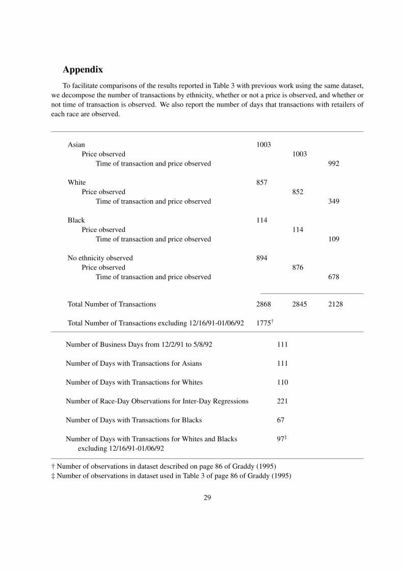
AppendixTo facilitate comparisons of the results reported in Table 3 with previous work using the same dataset,
we decompose the number of transactions by ethnicity, whether or not a price is observed, and whether ornot time of transaction is observed. We also report the number of days that transactions with retailers ofeach race are observed.
Asian 1003Price observed 1003
Time of transaction and price observed 992
White 857Price observed 852
Time of transaction and price observed 349
Black 114Price observed 114
Time of transaction and price observed 109
No ethnicity observed 894Price observed 876
Time of transaction and price observed 678
Total Number of Transactions 2868 2845 2128
Total Number of Transactions excluding 12/16/91-01/06/92 1775†
Number of Business Days from 12/2/91 to 5/8/92 111
Number of Days with Transactions for Asians 111
Number of Days with Transactions for Whites 110
Number of Race-Day Observations for Inter-Day Regressions 221
Number of Days with Transactions for Blacks 67
Number of Days with Transactions for Whites and Blacks 97‡
excluding 12/16/91-01/06/92
† Number of observations in dataset described on page 86 of Graddy (1995)‡ Number of observations in dataset used in Table 3 of page 86 of Graddy (1995)
29