Embed Size (px)
Citation preview
Introductory Numerical Analysis
Lecture Notes
Sudipta Mallik
May 4, 2018
Contents
1 Introduction to ≈ 11.1 Floating Point Numbers . . . . . . . . . . . . . . . . . . . . . . . . . . . . . 11.2 Computational Errors . . . . . . . . . . . . . . . . . . . . . . . . . . . . . . 21.3 Algorithm . . . . . . . . . . . . . . . . . . . . . . . . . . . . . . . . . . . . . 31.4 Calculus Review . . . . . . . . . . . . . . . . . . . . . . . . . . . . . . . . . . 3
2 Root Finding 52.1 Bisection Method . . . . . . . . . . . . . . . . . . . . . . . . . . . . . . . . . 52.2 Fixed Point Iteration . . . . . . . . . . . . . . . . . . . . . . . . . . . . . . . 82.3 Newton-Raphson Method . . . . . . . . . . . . . . . . . . . . . . . . . . . . 132.4 Order of Convergence . . . . . . . . . . . . . . . . . . . . . . . . . . . . . . . 16
3 Interpolation 183.1 Lagrange Polynomials . . . . . . . . . . . . . . . . . . . . . . . . . . . . . . 193.2 Cubic Spline Interpolation . . . . . . . . . . . . . . . . . . . . . . . . . . . . 23
4 Numerical Differentiation and Integration 264.1 Numerical Differentiation . . . . . . . . . . . . . . . . . . . . . . . . . . . . . 264.2 Elements of Numerical Integration . . . . . . . . . . . . . . . . . . . . . . . . 304.3 Composite Numerical Integration . . . . . . . . . . . . . . . . . . . . . . . . 33
5 Differential Equations 365.1 Euler’s Method . . . . . . . . . . . . . . . . . . . . . . . . . . . . . . . . . . 365.2 Higher-order Taylor’s Method . . . . . . . . . . . . . . . . . . . . . . . . . . 395.3 Runge-Kutta Method . . . . . . . . . . . . . . . . . . . . . . . . . . . . . . . 41
6 Linear Algebra 456.1 Introduction to Linear Algebra . . . . . . . . . . . . . . . . . . . . . . . . . 456.2 Systems of Linear Equations: Gaussian Elimination . . . . . . . . . . . . . . 486.3 Jacobi and Gauss-Seidel Methods . . . . . . . . . . . . . . . . . . . . . . . . 526.4 Eigenvalues: Power Method . . . . . . . . . . . . . . . . . . . . . . . . . . . 55
7 Additional Topics 587.1 Parabolic PDE: Heat Equation . . . . . . . . . . . . . . . . . . . . . . . . . 587.2 Least Squares Approximation . . . . . . . . . . . . . . . . . . . . . . . . . . 607.3 Elliptic PDE: Laplace Equation . . . . . . . . . . . . . . . . . . . . . . . . . 62
Numerical Analysis Sudipta Mallik
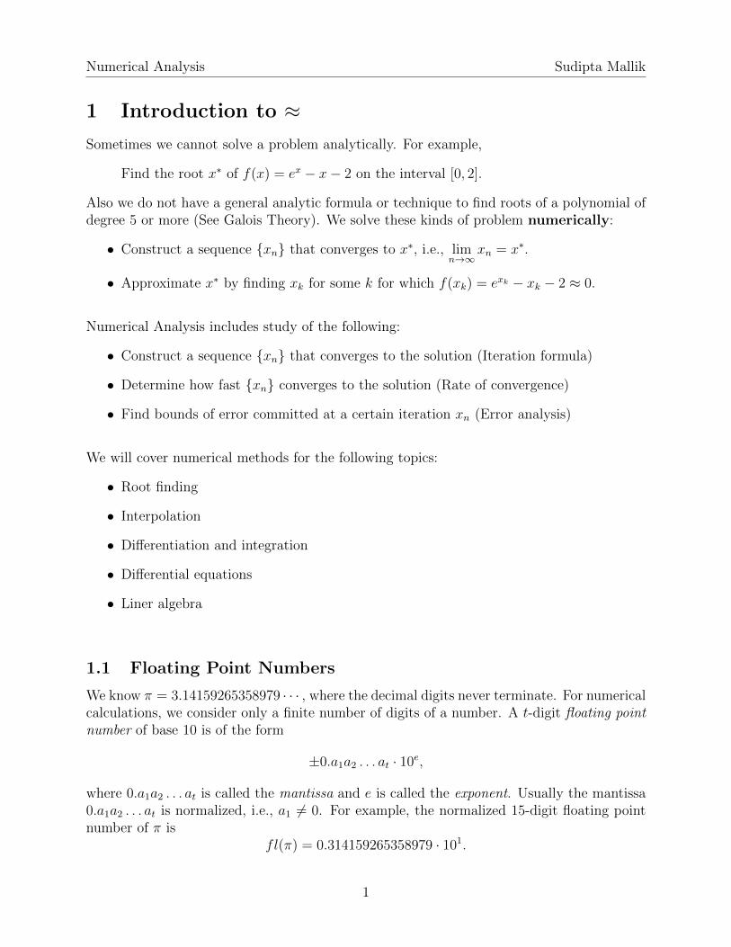
1 Introduction to ≈Sometimes we cannot solve a problem analytically. For example,
Find the root x∗ of f(x) = ex − x− 2 on the interval [0, 2].
Also we do not have a general analytic formula or technique to find roots of a polynomial ofdegree 5 or more (See Galois Theory). We solve these kinds of problem numerically:
• Construct a sequence {xn} that converges to x∗, i.e., limn→∞
xn = x∗.
• Approximate x∗ by finding xk for some k for which f(xk) = exk − xk − 2 ≈ 0.
Numerical Analysis includes study of the following:
• Construct a sequence {xn} that converges to the solution (Iteration formula)
• Determine how fast {xn} converges to the solution (Rate of convergence)
• Find bounds of error committed at a certain iteration xn (Error analysis)
We will cover numerical methods for the following topics:
• Root finding
• Interpolation
• Differentiation and integration
• Differential equations
• Liner algebra
1.1 Floating Point Numbers
We know π = 3.14159265358979 · · · , where the decimal digits never terminate. For numericalcalculations, we consider only a finite number of digits of a number. A t-digit floating pointnumber of base 10 is of the form
±0.a1a2 . . . at · 10e,
where 0.a1a2 . . . at is called the mantissa and e is called the exponent. Usually the mantissa0.a1a2 . . . at is normalized, i.e., a1 6= 0. For example, the normalized 15-digit floating pointnumber of π is
fl(π) = 0.314159265358979 · 101.
1
Numerical Analysis Sudipta Mallik
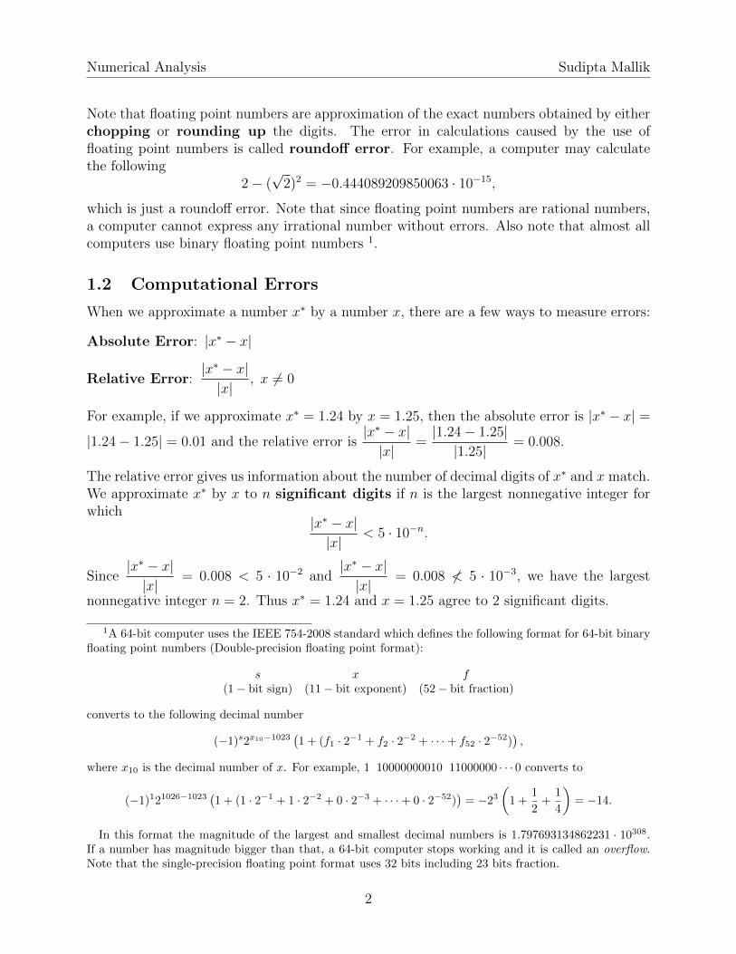
Note that floating point numbers are approximation of the exact numbers obtained by eitherchopping or rounding up the digits. The error in calculations caused by the use offloating point numbers is called roundoff error. For example, a computer may calculatethe following
2− (√
2)2 = −0.444089209850063 · 10−15,
which is just a roundoff error. Note that since floating point numbers are rational numbers,a computer cannot express any irrational number without errors. Also note that almost allcomputers use binary floating point numbers 1.
1.2 Computational Errors
When we approximate a number x∗ by a number x, there are a few ways to measure errors:
Absolute Error: |x∗ − x|
Relative Error:|x∗ − x||x|
, x 6= 0
For example, if we approximate x∗ = 1.24 by x = 1.25, then the absolute error is |x∗ − x| =
|1.24− 1.25| = 0.01 and the relative error is|x∗ − x||x|
=|1.24− 1.25||1.25|
= 0.008.
The relative error gives us information about the number of decimal digits of x∗ and x match.We approximate x∗ by x to n significant digits if n is the largest nonnegative integer forwhich
|x∗ − x||x|
< 5 · 10−n.
Since|x∗ − x||x|
= 0.008 < 5 · 10−2 and|x∗ − x||x|
= 0.008 ≮ 5 · 10−3, we have the largest
nonnegative integer n = 2. Thus x∗ = 1.24 and x = 1.25 agree to 2 significant digits.
1A 64-bit computer uses the IEEE 754-2008 standard which defines the following format for 64-bit binaryfloating point numbers (Double-precision floating point format):
s x f(1− bit sign) (11− bit exponent) (52− bit fraction)
converts to the following decimal number
(−1)s2x10−1023(1 + (f1 · 2−1 + f2 · 2−2 + · · ·+ f52 · 2−52)
),
where x10 is the decimal number of x. For example, 1 10000000010 11000000 · · · 0 converts to
(−1)121026−1023(1 + (1 · 2−1 + 1 · 2−2 + 0 · 2−3 + · · ·+ 0 · 2−52)
)= −23
(1 +
1
2+
1
4
)= −14.
In this format the magnitude of the largest and smallest decimal numbers is 1.797693134862231 · 10308.If a number has magnitude bigger than that, a 64-bit computer stops working and it is called an overflow.Note that the single-precision floating point format uses 32 bits including 23 bits fraction.
2
Numerical Analysis Sudipta Mallik
1.3 Algorithm
An algorithm is a set of ordered logical operations that applies to a problem defined by aset of data (input data) to produce a solution (output data). An algorithm is usually writtenin an informal way (pseudocode) before writing it with syntax of a computer language suchas C, Java, Python etc. The following is an example of a pseudocode to find n!:
Algorithm you-name-itInput: nonnegative integer nOutput: n!fact = 1for i =2 to n
fact = fact ∗ iend forreturn fact
Stopping criteria: Sometimes we need a stopping criteria to terminate an algorithm. Forexample, when an algorithm approximates a solution x∗ by constructing a sequence {xn},the algorithm needs to stop after finding xk for some k. There is no universal stoppingcriteria as it depends on the problem, acceptable error (i.e., error < tolerance, say 10−4), themaximum number of iterations etc.
1.4 Calculus Review
You should revise the limit definitions of the derivative and the Riemann integral of a func-tion from a standard text book. The following are some theorems which will be used later.
Theorem. Let f be a differentiable function on [a, b].
• f is increasing on [a, b] if and only if f ′(x) > 0 for all x ∈ [a, b].
• If f has a local maximum or minimum value at c, then f ′(c) = 0 (c is a criticalnumber).
• If f ′(c) = 0 and f ′′(c) < 0, then f(c) is a local maximum value.
• If f ′(c) = 0 and f ′′(c) > 0, then f(c) is a local minimum value.
Theorem. Let f be a continuous function on [a, b]. If f(c) is the absolute maximum orminimum value f on [a, b], then either f ′(c) does not exist or f ′(c) = 0 or c = a or c = b.
3
Numerical Analysis Sudipta Mallik
Intermediate Value Theorem: Let f be a function such that
(i) f is continuous on [a, b], and
(ii) N is a number between f(a) and f(b).
Then there is at least one number c in (a, b) such that f(c) = N .
In the particular case when f(a)f(b) < 0, i.e., f(a) and f(b) are of opposite signs, there isat least one root c of f in (a, b).
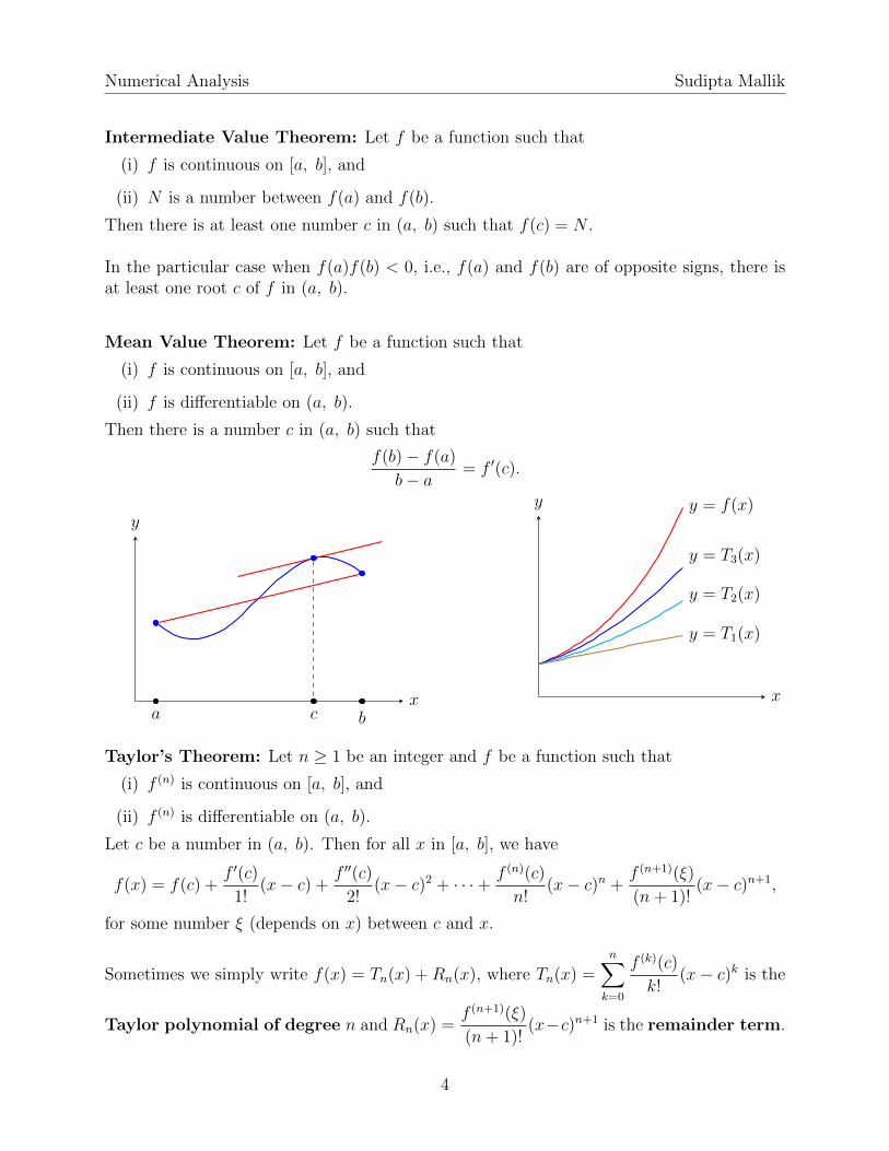
Mean Value Theorem: Let f be a function such that
(i) f is continuous on [a, b], and
(ii) f is differentiable on (a, b).
Then there is a number c in (a, b) such that
f(b)− f(a)
b− a= f ′(c).
x
y
a bcx
y y = f(x)
y = T3(x)
y = T2(x)
y = T1(x)
Taylor’s Theorem: Let n ≥ 1 be an integer and f be a function such that
(i) f (n) is continuous on [a, b], and
(ii) f (n) is differentiable on (a, b).
Let c be a number in (a, b). Then for all x in [a, b], we have
f(x) = f(c) +f ′(c)
1!(x− c) +
f ′′(c)
2!(x− c)2 + · · ·+ f (n)(c)
n!(x− c)n +
f (n+1)(ξ)
(n+ 1)!(x− c)n+1,
for some number ξ (depends on x) between c and x.
Sometimes we simply write f(x) = Tn(x) + Rn(x), where Tn(x) =n∑k=0
f (k)(c)
k!(x− c)k is the
Taylor polynomial of degree n and Rn(x) =f (n+1)(ξ)
(n+ 1)!(x−c)n+1 is the remainder term.
4
Numerical Analysis Sudipta Mallik
2 Root Finding
In this chapter we will find roots of a given function f , i.e., x∗ for which f(x∗) = 0.
2.1 Bisection Method
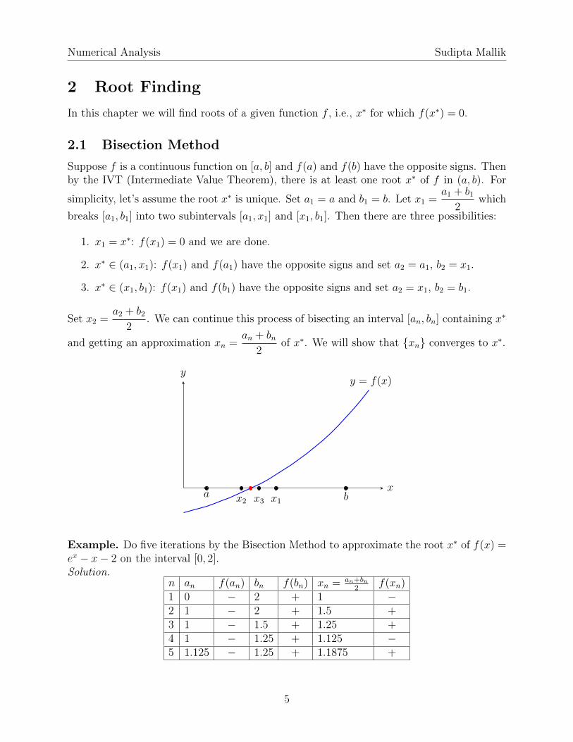
Suppose f is a continuous function on [a, b] and f(a) and f(b) have the opposite signs. Thenby the IVT (Intermediate Value Theorem), there is at least one root x∗ of f in (a, b). For
simplicity, let’s assume the root x∗ is unique. Set a1 = a and b1 = b. Let x1 =a1 + b1
2which
breaks [a1, b1] into two subintervals [a1, x1] and [x1, b1]. Then there are three possibilities:
1. x1 = x∗: f(x1) = 0 and we are done.
2. x∗ ∈ (a1, x1): f(x1) and f(a1) have the opposite signs and set a2 = a1, b2 = x1.
3. x∗ ∈ (x1, b1): f(x1) and f(b1) have the opposite signs and set a2 = x1, b2 = b1.
Set x2 =a2 + b2
2. We can continue this process of bisecting an interval [an, bn] containing x∗
and getting an approximation xn =an + bn
2of x∗. We will show that {xn} converges to x∗.
x
yy = f(x)
a bx1x2 x3
Example. Do five iterations by the Bisection Method to approximate the root x∗ of f(x) =ex − x− 2 on the interval [0, 2].Solution.
n an f(an) bn f(bn) xn = an+bn2
f(xn)1 0 − 2 + 1 −2 1 − 2 + 1.5 +3 1 − 1.5 + 1.25 +4 1 − 1.25 + 1.125 −5 1.125 − 1.25 + 1.1875 +
5
Numerical Analysis Sudipta Mallik
Since |x5 − x4| = |1.1875 − 1.125| = 0.0625 < 0.1 = 10−1, we can (roughly) say that theroot is x5 = 1.1875 correct to one decimal place. But why roughly?
If xn is correct to t decimal places, then |x∗ − xn| < 10−t. But the converse is not true.
For example, x∗ = 1.146193 is correct to 6 decimal places (believe me!). So x11 = 1.145507 isonly correct to 2 decimal places but |x∗−x11| < 10−3. Similarly if x∗ = 1.000 is approximatedby x = 0.999, then |x∗−x| = 0.001 < 10−2. But x = 0.999 is not correct to any decimal placesof x∗ = 1.000. Also note that we computed |x5−x4|, not |x∗−x5| (which is not known for x∗).
It would be useful to know the number of iteration that guarantees to achieve a certainaccuracy of the root, say within 10−3. That is to find n for which |x∗ − xn| < 10−3, i.e.,x∗ − 10−3 < xn < x∗ + 10−3. So we have to find an upper bound of the absolute error forthe nth iteration xn.
The Maximum Error: Let εn be the absolute error for the nth iteration xn. Then
εn = |x∗ − xn| ≤b− a
2n.
Proof. Since x∗ ∈ [an, bn] and bn − an = (bn−1 − an−1)/2 for all n,
εn = |x∗ − xn| ≤bn − an
2=bn−1 − an−1
22= · · · = b1 − a1
2n=b− a
2n.
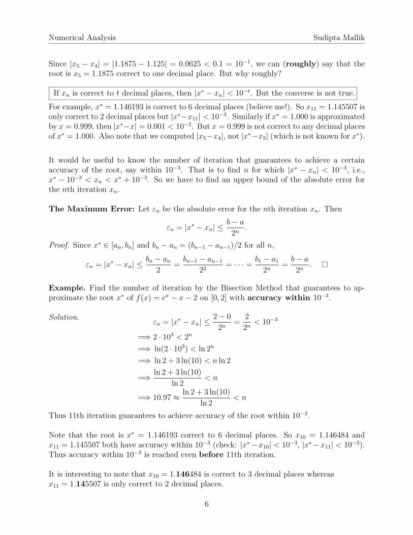
Example. Find the number of iteration by the Bisection Method that guarantees to ap-proximate the root x∗ of f(x) = ex − x− 2 on [0, 2] with accuracy within 10−3.
Solution.εn = |x∗ − xn| ≤
2− 0
2n=
2
2n< 10−3
=⇒ 2 · 103 < 2n
=⇒ ln(2 · 103) < ln 2n
=⇒ ln 2 + 3 ln(10) < n ln 2
=⇒ ln 2 + 3 ln(10)
ln 2< n
=⇒ 10.97 ≈ ln 2 + 3 ln(10)
ln 2< n
Thus 11th iteration guarantees to achieve accuracy of the root within 10−3.
Note that the root is x∗ = 1.146193 correct to 6 decimal places. So x10 = 1.146484 andx11 = 1.145507 both have accuracy within 10−3 (check: |x∗−x10| < 10−3, |x∗−x11| < 10−3).Thus accuracy within 10−3 is reached even before 11th iteration.
It is interesting to note that x10 = 1.146484 is correct to 3 decimal places whereasx11 = 1.145507 is only correct to 2 decimal places.
6
Numerical Analysis Sudipta Mallik
Convergence: The sequence {xn} constructed by the bisection method converges to thesolution x∗ because
limn→∞
|x∗ − xn| ≤ limn→∞
b− a2n
= 0 =⇒ limn→∞
|x∗ − xn| = 0.
But it converges really slowly in comparison to other methods (See Section 2.4).
Algorithm Bisection-MethodInput: f(x) = ex − x− 2, interval [0, 2], tolerance 10−3, maximum number of iterations 50Output: an approximate root of f on [0, 2] within 10−3 or a message of failureset a = 0 and b = 2;xold = a;for i = 1 to 50
x = (a+ b)/2;if |x− xold| < 10−3 % checking required accuracy
FoundSolution= true; % donebreak; % leave for environment
end ifif f(a)f(x) < 0
a=a and b=xelse
a=x and b=bend ifxold = x; % update xold for the next iteration
end forif FoundSolution
return xelse
print ‘the required accuracy is not reached in 50 iterations’end if
7
Numerical Analysis Sudipta Mallik
2.2 Fixed Point Iteration
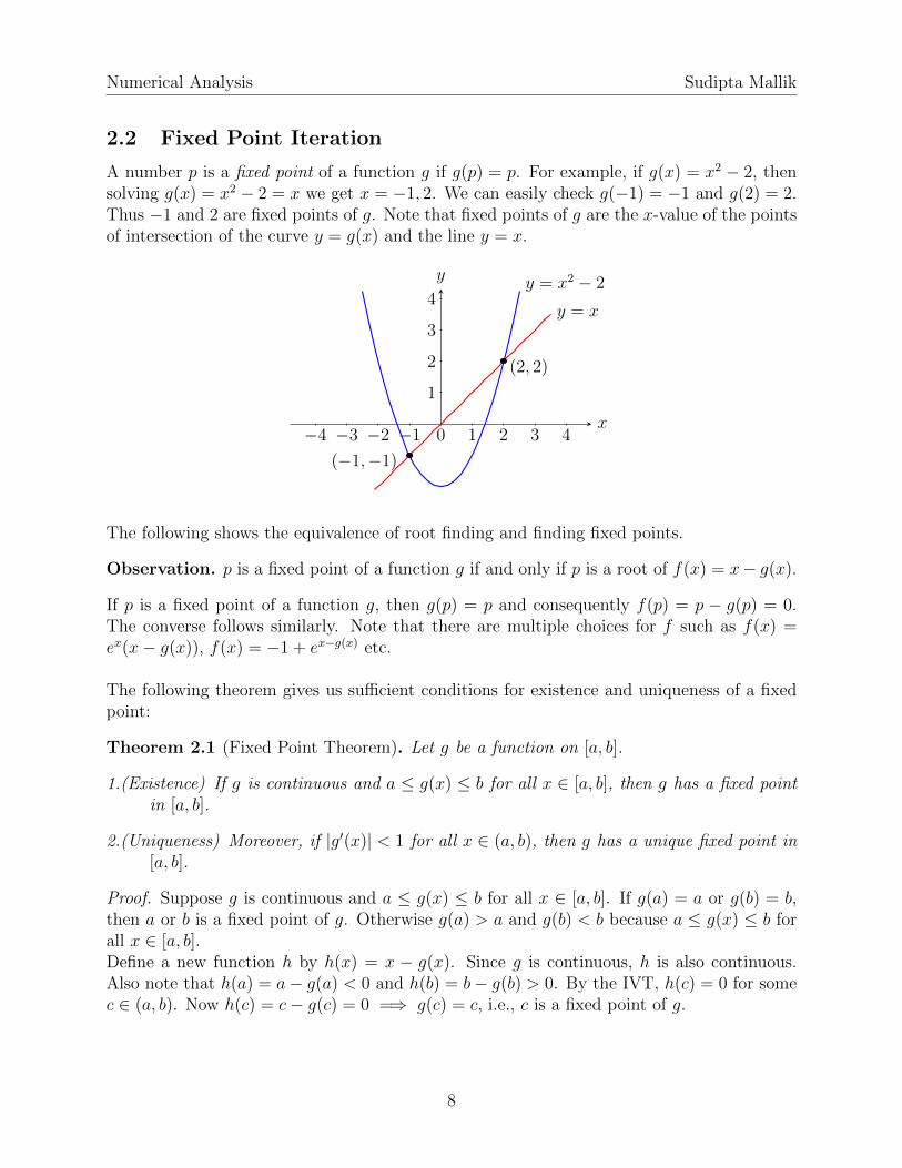
A number p is a fixed point of a function g if g(p) = p. For example, if g(x) = x2 − 2, thensolving g(x) = x2 − 2 = x we get x = −1, 2. We can easily check g(−1) = −1 and g(2) = 2.Thus −1 and 2 are fixed points of g. Note that fixed points of g are the x-value of the pointsof intersection of the curve y = g(x) and the line y = x.
x
y
−4 −3 −2 −1 0 1 2 3 4
1
2
3
4y = x2 − 2
y = x
(2, 2)
(−1,−1)
The following shows the equivalence of root finding and finding fixed points.
Observation. p is a fixed point of a function g if and only if p is a root of f(x) = x− g(x).
If p is a fixed point of a function g, then g(p) = p and consequently f(p) = p − g(p) = 0.The converse follows similarly. Note that there are multiple choices for f such as f(x) =ex(x− g(x)), f(x) = −1 + ex−g(x) etc.
The following theorem gives us sufficient conditions for existence and uniqueness of a fixedpoint:
Theorem 2.1 (Fixed Point Theorem). Let g be a function on [a, b].
1.(Existence) If g is continuous and a ≤ g(x) ≤ b for all x ∈ [a, b], then g has a fixed pointin [a, b].
2.(Uniqueness) Moreover, if |g′(x)| < 1 for all x ∈ (a, b), then g has a unique fixed point in[a, b].
Proof. Suppose g is continuous and a ≤ g(x) ≤ b for all x ∈ [a, b]. If g(a) = a or g(b) = b,then a or b is a fixed point of g. Otherwise g(a) > a and g(b) < b because a ≤ g(x) ≤ b forall x ∈ [a, b].Define a new function h by h(x) = x − g(x). Since g is continuous, h is also continuous.Also note that h(a) = a− g(a) < 0 and h(b) = b− g(b) > 0. By the IVT, h(c) = 0 for somec ∈ (a, b). Now h(c) = c− g(c) = 0 =⇒ g(c) = c, i.e., c is a fixed point of g.
8
Numerical Analysis Sudipta Mallik
Suppose |g′(x)| < 1 for all x ∈ (a, b). To show uniqueness of c, suppose d is another fixedpoint of g in [a, b]. WLOG let d > c. Applying the MVT on g on [c, d], we find t ∈ (c, d)such that
g(d)− g(c) = g′(t)(d− c).
Since |g′(x)| < 1 for all x ∈ (a, b),
g(d)− g(c) = g′(t)(d− c) < (d− c).
Since g(c) = c and g(d) = d, we have g(d)−g(c) = d−c which contradicts that g(d)−g(c) <(d− c).
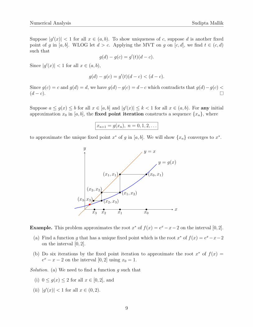
Suppose a ≤ g(x) ≤ b for all x ∈ [a, b] and |g′(x)| ≤ k < 1 for all x ∈ (a, b). For any initialapproximation x0 in [a, b], the fixed point iteration constructs a sequence {xn}, where
xn+1 = g(xn), n = 0, 1, 2, . . .
to approximate the unique fixed point x∗ of g in [a, b]. We will show {xn} converges to x∗.
x
y
y = g(x)
y = x
(x0, x1)(x1, x1)
(x1, x2)(x2, x2)
(x2, x3)(x3, x3)
x0x1x2x3
Example. This problem approximates the root x∗ of f(x) = ex−x−2 on the interval [0, 2].
(a) Find a function g that has a unique fixed point which is the root x∗ of f(x) = ex−x−2on the interval [0, 2].
(b) Do six iterations by the fixed point iteration to approximate the root x∗ of f(x) =ex − x− 2 on the interval [0, 2] using x0 = 1.
Solution. (a) We need to find a function g such that
(i) 0 ≤ g(x) ≤ 2 for all x ∈ [0, 2], and
(ii) |g′(x)| < 1 for all x ∈ (0, 2).
9
Numerical Analysis Sudipta Mallik
f(x) = ex−x−2 = 0 =⇒ x = ex−2. But g(x) = ex−2 does not satisfy (i) as g(0) = −2 < 0and also (ii) as g′(2) = e2 > 1. Note that
f(x) = ex − x− 2 = 0 =⇒ ex = x+ 2 =⇒ x = ln(x+ 2).
Take g(x) = ln(x + 2). Then g is an increasing function and g(0) = ln 2 > 0 andg(2) = ln 4 < 2. Thus 0 ≤ g(x) ≤ 2 for all x ∈ [0, 2]. Also |g′(x)| = 1
x+2≤ 1
2< 1 for all
x ∈ (0, 2). Thus g has a unique fixed point in [0, 2] which is the root x∗ of f(x) = ex− x− 2on the interval [0, 2].
(b) Use g(x) = ln(x+ 2) and x0 = 1.
n xn−1 xn = g(xn−1)1 1 1.09862 1.0986 1.13093 1.1309 1.14134 1.1413 1.14465 1.1446 1.14566 1.1457 1.1460
Since |x6 − x5| = |1.1460 − 1.1456| = 0.0004 < 0.001 = 10−3, we can say that the root isx6 = 1.1460 roughly correct to three decimal places (which is true indeed as x∗ = 1.146193).
The Maximum Error: Let εn be the absolute error for the nth iteration xn. Then
εn = |x∗ − xn| ≤kn max{x0 − a, b− x0} and
εn = |x∗ − xn| ≤kn
1− k|x1 − x0|.
Proof. Applying the MVT on g on [x∗, xn−1], we find ξn−1 ∈ (x∗, xn−1) such thatg(x∗)− g(xn−1) = g′(ξn−1)(x
∗ − xn−1). Then
|x∗ − xn| = |g(x∗)− g(xn−1)| = |g′(ξn−1)||x∗ − xn−1| ≤ k|x∗ − xn−1|.
Continuing this process, we get
|x∗ − xn| ≤ k|x∗ − xn−1| ≤ k2|x∗ − xn−2| ≤ · · · ≤ kn|x∗ − x0|.
Since x∗, x0 ∈ (a, b), we have |x∗ − x0| ≤ max{x0 − a, b − x0}. Thus εn = |x∗ − xn| ≤kn max{x0 − a, b− x0}.
Note that similarly applying the MVT on g on [xn, xn+1], we can show that
|xn+1 − xn| ≤ kn|x1 − x0|.
10
Numerical Analysis Sudipta Mallik
For the other bound, let m > n ≥ 0. Then
|xm − xn| = |xm − xm−1 + xm−1 − xm−2 + xm−2 − · · ·+ xn+1 − xn|≤ |xm − xm−1|+ |xm−1 − xm−2|+ · · ·+ |xn+1 − xn|≤ km−1|x∗ − x0|+ km−2|x∗ − x0|+ · · ·+ kn|x∗ − x0|≤ kn|x∗ − x0|(1 + k + · · ·+ km−n−1)
≤ kn|x∗ − x0|m−n−1∑i=0
ki
Thus
limm→∞
|xm − xn| ≤ limm→∞
kn|x∗ − x0|m−n−1∑i=0
ki = kn|x∗ − x0|∞∑i=0
ki
=⇒ |x∗ − xn| ≤ kn|x∗ − x0|∞∑i=0
ki =kn
1− k|x1 − x0| (as 0 < k < 1).
Convergence: The sequence {xn} constructed by the fixed point iteration converges to theunique fixed point x∗ irrespective of choice of the initial approximation x0 because
limn→∞
|x∗ − xn| ≤ limn→∞
kn max{x0 − a, b− x0} = 0 (as 0 < k < 1) =⇒ limn→∞
|x∗ − xn| = 0.
It converges really fast when k is close to 0.
Example. Find the number of iteration by the fixed point iteration that guarantees to ap-proximate the root x∗ of f(x) = ex−x−2 on [0, 2] using x0 = 1 with accuracy within 10−3.
Solution. Consider g(x) = ln(x+ 2) on [0, 2] where |g′(x)| ≤ 12
= k < 1 for all x ∈ (0, 2).
εn = |x∗ − xn| ≤ kn max{x0 − a, b− x0} =
(1
2
)n· 1 < 10−3
=⇒ 103 < 2n
=⇒ ln 103 < ln 2n
=⇒ 3 ln 10 < n ln 2
=⇒ 3 ln 10
ln 2≈ 9.97 < n
Thus 10th iteration guarantees to achieve accuracy of the root within 10−3. But note that|x∗ − x5| = |1.1461− 1.1457| = 0.0004 < 10−3. So Thus accuracy within 10−3 is reached at5th iteration (way before 10th iteration). Also note that the other bound of εn = |x∗−xn| ≤kn
1−k |x1 − x0| gives 10.94 < n which does not improve our answer.
11
Numerical Analysis Sudipta Mallik
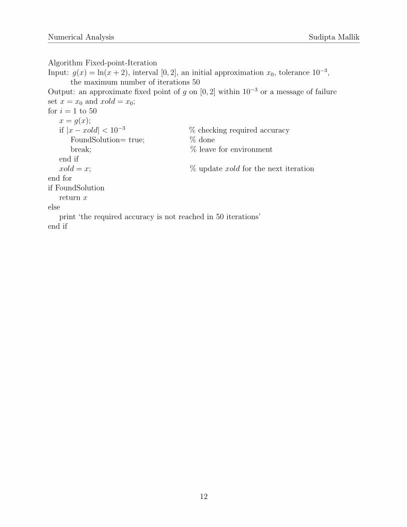
Algorithm Fixed-point-IterationInput: g(x) = ln(x+ 2), interval [0, 2], an initial approximation x0, tolerance 10−3,
the maximum number of iterations 50Output: an approximate fixed point of g on [0, 2] within 10−3 or a message of failureset x = x0 and xold = x0;for i = 1 to 50
x = g(x);if |x− xold| < 10−3 % checking required accuracy
FoundSolution= true; % donebreak; % leave for environment
end ifxold = x; % update xold for the next iteration
end forif FoundSolution
return xelse
print ‘the required accuracy is not reached in 50 iterations’end if
12
Numerical Analysis Sudipta Mallik
2.3 Newton-Raphson Method
Suppose f is a function with a unique root x∗ in [a, b]. Assume f ′′ is continuous in [a, b].To find x∗, let x0 be a “good” initial approximation (i.e., |x∗ − x0|2 ≈ 0) where f ′(x0) 6= 0.Using Taylor’s Theorem on f about x0, we get
f(x) = f(x0) +f ′(x0)
1!(x− x0) +
f ′′(ξ)
2!(x− x0)2,
for some number ξ (depends on x) between x0 and x. Plugging x = x∗, we get
0 = f(x∗) = f(x0) +f ′(x0)
1!(x∗ − x0) +
f ′′(ξ)
2!(x∗ − x0)2
=⇒ f(x0) +f ′(x0)
1!(x∗ − x0) = −f
′′(ξ)
2!(x∗ − x0)2 ≈ 0 (since |x∗ − x0|2 ≈ 0)
Now solving for x∗, we get
x∗ ≈ x0 −f(x0)
f ′(x0).
So x1 = x0 − f(x0)f ′(x0)
is an approximation to x∗. Using x1, similarly we get x2 = x1 − f(x1)f ′(x1)
.
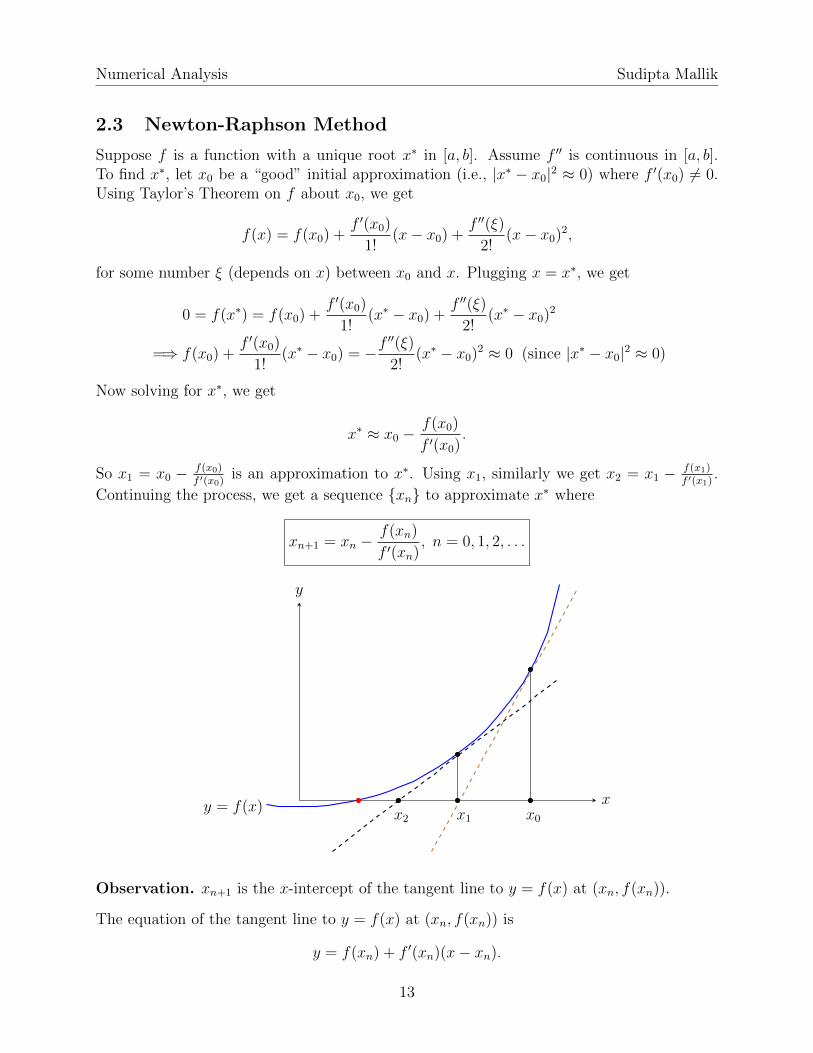
Continuing the process, we get a sequence {xn} to approximate x∗ where
xn+1 = xn −f(xn)
f ′(xn), n = 0, 1, 2, . . .
x
y
y = f(x)x0x1x2
Observation. xn+1 is the x-intercept of the tangent line to y = f(x) at (xn, f(xn)).
The equation of the tangent line to y = f(x) at (xn, f(xn)) is
y = f(xn) + f ′(xn)(x− xn).
13
Numerical Analysis Sudipta Mallik
For the x-intercept, y = 0. So
0 = f(xn) + f ′(xn)(x− xn) =⇒ x = xn −f(xn)
f ′(xn).
Thus xn+1 is the x-intercept of the tangent line to y = f(x) at (xn, f(xn)).
Note. We will show later that {xn} converges to x∗ for a good choice of an initial approxi-mation x0. If x0 is far from x∗, then {xn} may not converge to x∗.
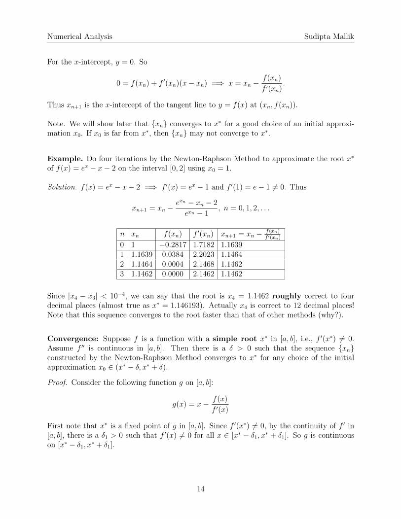
Example. Do four iterations by the Newton-Raphson Method to approximate the root x∗
of f(x) = ex − x− 2 on the interval [0, 2] using x0 = 1.
Solution. f(x) = ex − x− 2 =⇒ f ′(x) = ex − 1 and f ′(1) = e− 1 6= 0. Thus
xn+1 = xn −exn − xn − 2
exn − 1, n = 0, 1, 2, . . .
n xn f(xn) f ′(xn) xn+1 = xn − f(xn)f ′(xn)
0 1 −0.2817 1.7182 1.16391 1.1639 0.0384 2.2023 1.14642 1.1464 0.0004 2.1468 1.14623 1.1462 0.0000 2.1462 1.1462
Since |x4 − x3| < 10−4, we can say that the root is x4 = 1.1462 roughly correct to fourdecimal places (almost true as x∗ = 1.146193). Actually x4 is correct to 12 decimal places!Note that this sequence converges to the root faster than that of other methods (why?).
Convergence: Suppose f is a function with a simple root x∗ in [a, b], i.e., f ′(x∗) 6= 0.Assume f ′′ is continuous in [a, b]. Then there is a δ > 0 such that the sequence {xn}constructed by the Newton-Raphson Method converges to x∗ for any choice of the initialapproximation x0 ∈ (x∗ − δ, x∗ + δ).
Proof. Consider the following function g on [a, b]:
g(x) = x− f(x)
f ′(x)
First note that x∗ is a fixed point of g in [a, b]. Since f ′(x∗) 6= 0, by the continuity of f ′ in[a, b], there is a δ1 > 0 such that f ′(x) 6= 0 for all x ∈ [x∗ − δ1, x∗ + δ1]. So g is continuouson [x∗ − δ1, x∗ + δ1].
14
Numerical Analysis Sudipta Mallik
The convergence follows by that of the Fixed Point Iteration of g on [x∗ − δ, x∗ + δ] if wecan show that there is a positive δ < δ1 such that (i) x∗ − δ ≤ g(x) ≤ x∗ + δ for allx ∈ [x∗ − δ, x∗ + δ] and (ii) |g′(x)| < 1 for all x ∈ (x∗ − δ, x∗ + δ). To prove (ii), note that
g′(x) = 1− f ′(x)f ′(x)− f(x)f ′′(x)
(f ′(x))2=f(x)f ′′(x)
(f ′(x))2
=⇒ g′(x∗) =f(x∗)f ′′(x∗)
(f ′(x∗))2= 0 (since f(x∗) = 0, f ′(x∗) 6= 0)
Since g′(x∗) = 0, by the continuity of g′ in [x∗− δ, x∗+ δ], there is a positive δ < δ1 such that|g′(x)| < 1 for all x ∈ (x∗ − δ, x∗ + δ). So we have (ii). To show (i), take x ∈ [x∗ − δ, x∗ + δ].By the MVT on g, we have g(x∗)− g(x) = g′(ξ)(x∗− x) for some ξ between x and x∗. Thus
|x∗ − g(x)| = |g(x∗)− g(x)| = |g′(ξ)||x∗ − x| < |x∗ − x|.
Since x ∈ [x∗ − δ, x∗ + δ], i.e., |x∗ − x| ≤ δ, we have |x∗ − g(x)| < |x∗ − x| ≤ δ, i.e.,x∗ − δ ≤ g(x) ≤ x∗ + δ.
Note that if the root x∗ of f is not simple, i.e., f ′(x∗) = 0, then this proof does not work butstill {xn} may converge to x∗. For multiple root x∗ of f we use a modified Newton-Raphsoniteration formula .
The Secant Method: In the iteration formula by the Newton-Raphson Method
xn+1 = xn −f(xn)
f ′(xn), n = 0, 1, 2, . . . ,
we need to calculate the derivative f ′(xn) which may be difficult sometimes. To avoid suchcalculations, the Secant Method modifies the above formula by replacing f ′(xn) with itsapproximation. Note that
f ′(xn) = limx→xn
f(x)− f(xn)
x− xn.
If xn−1 is close to xn, then
f ′(xn) ≈ f(xn−1)− f(xn)
xn−1 − xn=f(xn)− f(xn−1)
xn − xn−1.
Thus
xn+1 = xn −f(xn)
f ′(xn)≈ xn −
f(xn)f(xn)−f(xn−1)
xn−xn−1
= xn −(xn − xn−1)f(xn)
f(xn)− f(xn−1).
Thus the iteration formula by the Secant Method is
xn+1 = xn −(xn − xn−1)f(xn)
f(xn)− f(xn−1), n = 1, 2, 3, . . .
Note that geometrically xn+1 is the x-intercept of the secant line joining (xn, f(xn)) and(xn−1, f(xn−1)). Also note that the convergence of the sequence {xn} by the Secant Methodis slower than that of the Newton-Raphson Method.
15
Numerical Analysis Sudipta Mallik
2.4 Order of Convergence
In the preceding three sections we learned techniques to construct a sequence {xn} thatconverges to the root x∗ of a function. But the speed of their convergence are different. Inthis section we will compare them by their order of convergence.
Definition. The convergence of a sequence {xn} to x∗ is of order p if
limn→∞
|xn+1 − x∗||xn − x∗|p
= limn→∞
εn+1
εpn= c,
for some constant c > 0.
For higher order convergence (i.e., larger p), the sequence converges more rapidly. The rateof convergence is called linear, quadratic, and superlinear if p = 1, p = 2, and 1 < p < 2respectively. We say {xn} converges linearly, quadratically, or superlinearly to x∗. Inquadratic convergence, we have εn+1 ≈ cε2n and then accuracy of xn to x∗ gets roughlydouble at each iteration.
Example. The sequence { 12n} converges linearly to 0.
limn→∞
|2−(n+1) − 0||2−n − 0|p
= limn→∞
2pn−n−1 =
0 if p < 1
1/2 if p = 1
∞ if p > 1.
Example. The order of convergence of the Bisection Method is linear.
Recall that
εn = |x∗ − xn| ≤b− a
2n.
So the rate of convergence of the sequence {xn} is similar to (at least) that of { 12n}. We
denote this by xn = x∗ +O( 12n
). Since { 12n} converges linearly, {xn} also converges linearly.
Example. The order of convergence of the Fixed Point Iteration is linear when g′(x∗) 6= 0.
Consider the sequence {xn}, where xn+1 = g(xn), that converges to x∗ where g′(x∗) 6= 0. Wehave shown before by applying the MVT on g on [x∗, xn], that we find ξn ∈ (x∗, xn) suchthat
x∗ − xn+1 = g(x∗)− g(xn) = g′(ξn)(x∗ − xn).
Since {xn} converges to x∗ and ξn ∈ (x∗, xn), {ξn} also converges to x∗. Then
limn→∞
|x∗ − xn+1||x∗ − xn|
= limn→∞
|g′(ξn)| = |g′( limn→∞
ξn)| = |g′(x∗)| (Assuming continuity of g′).
16
Numerical Analysis Sudipta Mallik
Example. The order of convergence of the Newton-Raphson Method to find a simple rootis quadratic.
Recall that to find a simple root x∗ of f (i.e., f ′(x∗) 6= 0), we used the Fixed Point Iterationon
g(x) = x− f(x)
f ′(x)
for any choice of the initial approximation x0 ∈ (x∗ − δ, x∗ + δ) for small δ > 0. Also recallthat since f(x∗) = 0 and f ′(x∗) 6= 0, g′(x∗) = 0. By Taylor’s Theorem on g about x∗, we get
g(x) = g(x∗) +g′(x∗)
1!(x− x∗) +
g′′(ξ)
2!(x− x∗)2,
for some ξ between x and x∗. For x = xn, we get ξn between xn and x∗ such that
g(xn) = g(x∗) +g′(x∗)
1!(xn − x∗) +
g′′(ξn)
2!(xn − x∗)2
=⇒ xn+1 = x∗ +g′(x∗)
1!(xn − x∗) +
g′′(ξn)
2!(xn − x∗)2
=⇒ xn+1 − x∗ =g′′(ξn)
2!(xn − x∗)2 (since g′(x∗) = 0)
=⇒ limn→∞
|xn+1 − x∗||xn − x∗|2
= limn→∞
|g′′(ξn)|2!
=|g′′(
limn→∞
ξn
)|
2!(Assuming continuity of g′′)
Since {xn} converges to x∗ and ξn lies between xn and x∗, {ξn} also converges to x∗. Thus
limn→∞
|xn+1 − x∗||xn − x∗|2
=|g′′(x∗)|
2=|f ′′(x∗)|2|f ′(x∗)|
.
Note
1. If the root is not simple, the Newton-Raphson Method still may converge but theorder of convergence is not quadratic but linear. For example, to approximate thedouble root zero of f(x) = x2 using x0 = 1 by the Newton-Raphson Method, itconstructs the sequence { 1
2n} which converges to 0 linearly.
2. A modified Newton-Raphson Method to find a multiple root has linear convergence.
3. The order of convergence of the Secant Method is superlinear (p = (1+√
5)/2 ≈ 1.6)which is in between that of the Bisection Method and the Newton-Raphson Method.(Proof skipped)
17
Numerical Analysis Sudipta Mallik
3 Interpolation
Suppose we have a set of data in which for each xi you have yi:
x0 y0x1 y1x2 y2x3 y3...
...xn yn
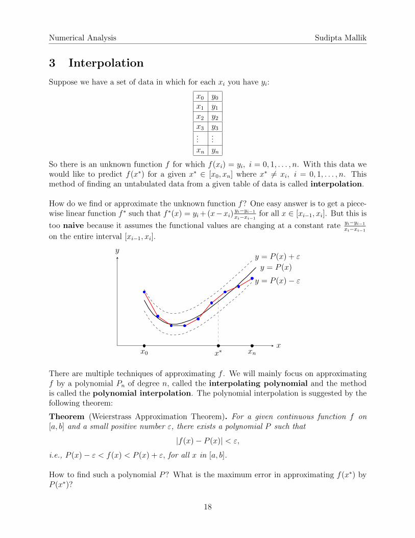
So there is an unknown function f for which f(xi) = yi, i = 0, 1, . . . , n. With this data wewould like to predict f(x∗) for a given x∗ ∈ [x0, xn] where x∗ 6= xi, i = 0, 1, . . . , n. Thismethod of finding an untabulated data from a given table of data is called interpolation.
How do we find or approximate the unknown function f? One easy answer is to get a piece-wise linear function f ∗ such that f ∗(x) = yi + (x−xi) yi−yi−1
xi−xi−1for all x ∈ [xi−1, xi]. But this is
too naive because it assumes the functional values are changing at a constant rate yi−yi−1
xi−xi−1
on the entire interval [xi−1, xi].
x
y
y = P (x)
y = P (x) + ε
y = P (x)− ε
x0 x∗ xn
There are multiple techniques of approximating f . We will mainly focus on approximatingf by a polynomial Pn of degree n, called the interpolating polynomial and the methodis called the polynomial interpolation. The polynomial interpolation is suggested by thefollowing theorem:
Theorem (Weierstrass Approximation Theorem). For a given continuous function f on[a, b] and a small positive number ε, there exists a polynomial P such that
|f(x)− P (x)| < ε,
i.e., P (x)− ε < f(x) < P (x) + ε, for all x in [a, b].
How to find such a polynomial P? What is the maximum error in approximating f(x∗) byP (x∗)?
18
Numerical Analysis Sudipta Mallik
3.1 Lagrange Polynomials
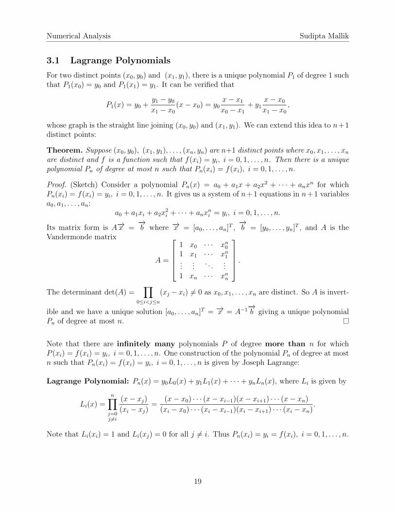
For two distinct points (x0, y0) and (x1, y1), there is a unique polynomial P1 of degree 1 suchthat P1(x0) = y0 and P1(x1) = y1. It can be verified that
P1(x) = y0 +y1 − y0x1 − x0
(x− x0) = y0x− x1x0 − x1
+ y1x− x0x1 − x0
,
whose graph is the straight line joining (x0, y0) and (x1, y1). We can extend this idea to n+1distinct points:
Theorem. Suppose (x0, y0), (x1, y1), . . . , (xn, yn) are n+1 distinct points where x0, x1, . . . , xnare distinct and f is a function such that f(xi) = yi, i = 0, 1, . . . , n. Then there is a uniquepolynomial Pn of degree at most n such that Pn(xi) = f(xi), i = 0, 1, . . . , n.
Proof. (Sketch) Consider a polynomial Pn(x) = a0 + a1x + a2x2 + · · · + anx
n for whichPn(xi) = f(xi) = yi, i = 0, 1, . . . , n. It gives us a system of n+1 equations in n+1 variablesa0, a1, . . . , an:
a0 + a1xi + a2x2i + · · ·+ anx
ni = yi, i = 0, 1, . . . , n.
Its matrix form is A−→x =−→b where −→x = [a0, . . . , an]T ,
−→b = [y0, . . . , yn]T , and A is the
Vandermonde matrix
A =
1 x0 · · · xn01 x1 · · · xn1...
.... . .
...1 xn · · · xnn
.The determinant det(A) =
∏0≤i<j≤n
(xj − xi) 6= 0 as x0, x1, . . . , xn are distinct. So A is invert-
ible and we have a unique solution [a0, . . . , an]T = −→x = A−1−→b giving a unique polynomial
Pn of degree at most n.
Note that there are infinitely many polynomials P of degree more than n for whichP (xi) = f(xi) = yi, i = 0, 1, . . . , n. One construction of the polynomial Pn of degree at mostn such that Pn(xi) = f(xi) = yi, i = 0, 1, . . . , n is given by Joseph Lagrange:
Lagrange Polynomial: Pn(x) = y0L0(x) + y1L1(x) + · · ·+ ynLn(x), where Li is given by
Li(x) =n∏j=0j 6=i
(x− xj)(xi − xj)
=(x− x0) · · · (x− xi−1)(x− xi+1) · · · (x− xn)
(xi − x0) · · · (xi − xi−1)(xi − xi+1) · · · (xi − xn).
Note that Li(xi) = 1 and Li(xj) = 0 for all j 6= i. Thus Pn(xi) = yi = f(xi), i = 0, 1, . . . , n.
19
Numerical Analysis Sudipta Mallik
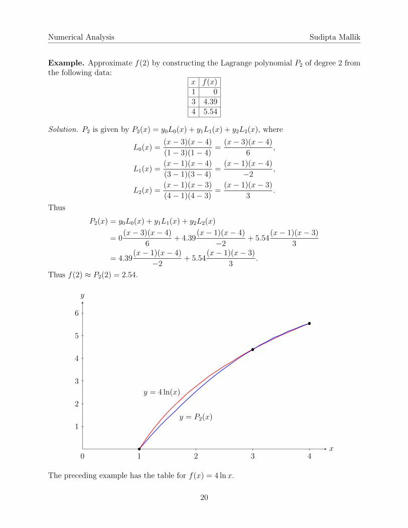
Example. Approximate f(2) by constructing the Lagrange polynomial P2 of degree 2 fromthe following data:
x f(x)1 03 4.394 5.54
Solution. P2 is given by P2(x) = y0L0(x) + y1L1(x) + y2L2(x), where
L0(x) =(x− 3)(x− 4)
(1− 3)(1− 4)=
(x− 3)(x− 4)
6,
L1(x) =(x− 1)(x− 4)
(3− 1)(3− 4)=
(x− 1)(x− 4)
−2,
L2(x) =(x− 1)(x− 3)
(4− 1)(4− 3)=
(x− 1)(x− 3)
3.
Thus
P2(x) = y0L0(x) + y1L1(x) + y2L2(x)
= 0(x− 3)(x− 4)
6+ 4.39
(x− 1)(x− 4)
−2+ 5.54
(x− 1)(x− 3)
3
= 4.39(x− 1)(x− 4)
−2+ 5.54
(x− 1)(x− 3)
3.
Thus f(2) ≈ P2(2) = 2.54.
x
y
1 2 3 4
1
2
3
4
5
6
0
y = 4 ln(x)
y = P2(x)
The preceding example has the table for f(x) = 4 lnx.
20
Numerical Analysis Sudipta Mallik
Maximum Error: If a function f that has continuous f (n+1) on [x0, xn] is interpolated bythe Lagrange polynomial Pn using n+ 1 points (x0, y0), (x1, y1), . . . , (xn, yn), then the erroris given by the following for each x ∈ [x0, xn]:
f(x)− Pn(x) =f (n+1)(ξ)
(n+ 1)!(x− x0)(x− x1) · · · (x− xn),
where ξ ∈ (x0, xn) depends on x.
Proof. (Sketch) If x = xi, i = 0, 1, . . . , n, then
f(xi)− Pn(xi) = 0 =f (n+1)(ξ)
(n+ 1)!(xi − x0)(xi − x1) · · · (xi − xn).
For a fixed x 6= xi, i = 0, 1, . . . , n, define a function g on [x0, xn] by
g(t) = f(t)− Pn(t)− [f(x)− Pn(x)]n∏j=0
(t− xj)(x− xj)
.
Verify that g(n+1) is continuous on [x0, xn] and g is zero at x, x0, x1, . . . , xn. Then by the Gen-eralized Rolle’s Theorem, g(n+1)(ξ) = 0 for some ξ ∈ (x0, xn) which implies (steps skipped)
f (n+1)(ξ)− 0− [f(x)− Pn(x)](n+ 1)!n∏j=0
(x− xj)= 0.
Now solving for f(x), we get
f(x)− Pn(x) =f (n+1)(ξ)
(n+ 1)!(x− x0)(x− x1) · · · (x− xn).
So the maximum error is given by
|f(x)− Pn(x)| ≤ MK
(n+ 1)!
where M = maxx∈[x0,xn]
|f (n+1)(x)| and K = maxx∈[x0,xn]
|(x− x0)(x− x1) · · · (x− xn)|.
This error bound does not have a practical application as f is unknown. But it shows thatthe error decreases when we take more points n (most of the times!).
Note that if f is a polynomial of degree at most n, then f (n+1) = 0 and consequently M = 0giving no error.
21
Numerical Analysis Sudipta Mallik
Example. Find the maximum error in approximating f(x) = 4 lnx on [1, 4] by the Lagrangepolynomial P2 using points x = 1, 3, 4.
Solution. Since |f ′′′(x)| = 8/x3 is decreasing on [1, 4], M = maxx∈[1,4]
|f ′′′(x)| = |f ′′′(1)| = 8.
Now we find extremum values of g(x) = (x− 1)(x− 3)(x− 4) = x3 − 8x2 + 19x− 12.
g′(x) = 3x2 − 16x+ 19 = 0 =⇒ x = (8±√
7)/3.
Note that (8±√
7)/3 ∈ [1, 4] and
g((8 +√
7)/3) = (20− 14√
7)/27
g((8−√
7)/3) = (20 + 14√
7)/27
g(1) = 0
g(4) = 0.
Since |g((8−√
7)/3)| > |g((8 +√
7)/3)|,
K = maxx∈[1,4]
|(x− 1)(x− 3)(x− 4)| = (20 + 14√
7)/27.
Thus the maximum error is
MK
(n+ 1)!=
8 · (20 + 14√
7)/27
3!= 2.81.
The last example has the table for f(x) = 4 lnx. So f(2) = 4 ln 2 = 2.77 and the absoluteerror is |P2(2) − f(2)| = |2.54 − 2.77| = 0.23. But approximating f(x) by P2(x) for anyx ∈ [1, 4] will have the maximum error 2.81.
Note that another construction of the unique polynomial Pn of degree at most n such thatPn(xi) = f(xi), i = 0, 1, . . . , n is given by Issac Newton:
Pn(x) = a0 + a1(x− x0) + a2(x− x0)(x− x1) + · · ·+ an(x− x0) · · · (x− xn−1),
where ai, i = 0, . . . , n are found by Divided Differences.
22
Numerical Analysis Sudipta Mallik
3.2 Cubic Spline Interpolation
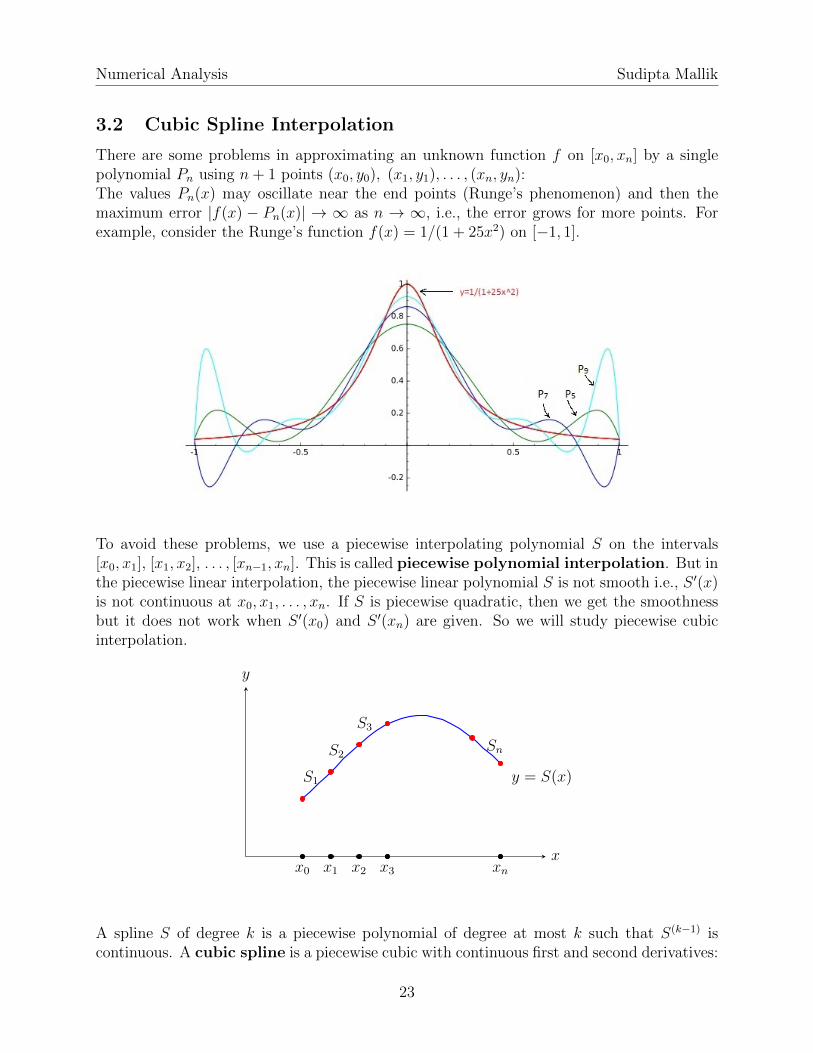
There are some problems in approximating an unknown function f on [x0, xn] by a singlepolynomial Pn using n+ 1 points (x0, y0), (x1, y1), . . . , (xn, yn):The values Pn(x) may oscillate near the end points (Runge’s phenomenon) and then themaximum error |f(x) − Pn(x)| → ∞ as n → ∞, i.e., the error grows for more points. Forexample, consider the Runge’s function f(x) = 1/(1 + 25x2) on [−1, 1].
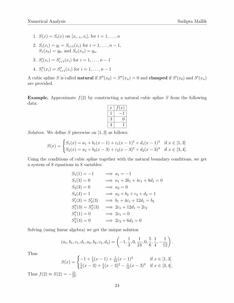
To avoid these problems, we use a piecewise interpolating polynomial S on the intervals[x0, x1], [x1, x2], . . . , [xn−1, xn]. This is called piecewise polynomial interpolation. But inthe piecewise linear interpolation, the piecewise linear polynomial S is not smooth i.e., S ′(x)is not continuous at x0, x1, . . . , xn. If S is piecewise quadratic, then we get the smoothnessbut it does not work when S ′(x0) and S ′(xn) are given. So we will study piecewise cubicinterpolation.
x
y
y = S(x)S1
S2
S3
Sn
x0 x1 x2 x3 xn
A spline S of degree k is a piecewise polynomial of degree at most k such that S(k−1) iscontinuous. A cubic spline is a piecewise cubic with continuous first and second derivatives:
23
Numerical Analysis Sudipta Mallik
1. S(x) = Si(x) on [xi−1, xi], for i = 1, . . . , n
2. Si(xi) = yi = Si+1(xi) for i = 1, . . . , n− 1,S1(x0) = y0, and Sn(xn) = yn.
3. S ′i(xi) = S ′i+1(xi) for i = 1, . . . , n− 1
4. S ′′i (xi) = S ′′i+1(xi) for i = 1, . . . , n− 1
A cubic spline S is called natural if S ′′(x0) = S ′′(xn) = 0 and clamped if S ′(x0) and S ′(xn)are provided.
Example. Approximate f(2) by constructing a natural cubic spline S from the followingdata:
x f(x)1 −13 04 1
Solution. We define S piecewise on [1, 3] as follows:
S(x) =
{S1(x) = a1 + b1(x− 1) + c1(x− 1)2 + d1(x− 1)3 if x ∈ [1, 3]
S2(x) = a2 + b2(x− 3) + c2(x− 3)2 + d2(x− 3)3 if x ∈ [3, 4].
Using the conditions of cubic spline together with the natural boundary conditions, we geta system of 8 equations in 8 variables:
S1(1) = −1 =⇒ a1 = −1
S1(3) = 0 =⇒ a1 + 2b1 + 4c1 + 8d1 = 0
S2(3) = 0 =⇒ a2 = 0
S2(4) = 1 =⇒ a2 + b2 + c2 + d2 = 1
S ′1(3) = S ′2(3) =⇒ b1 + 4c1 + 12d1 = b2
S ′′1 (3) = S ′′2 (3) =⇒ 2c1 + 12d1 = 2c2
S ′′1 (1) = 0 =⇒ 2c1 = 0
S ′′2 (4) = 0 =⇒ 2c2 + 6d2 = 0
Solving (using linear algebra) we get the unique solution
(a1, b1, c1, d1, a2, b2, c2, d2) =
(−1,
1
3, 0,
1
24, 0,
5
6,1
4,− 1
12
).
Thus
S(x) =
{−1 + 1
3(x− 1) + 1
24(x− 1)3 if x ∈ [1, 3]
56(x− 3) + 1
4(x− 3)2 − 1
12(x− 3)3 if x ∈ [3, 4].
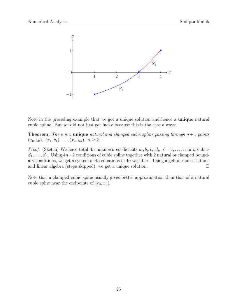
Thus f(2) ≈ S(2) = −1524
.
24
Numerical Analysis Sudipta Mallik
x
y
1 2 3 4
−1
0
1
S1
S2
Note in the preceding example that we got a unique solution and hence a unique naturalcubic spline. But we did not just get lucky because this is the case always:
Theorem. There is a unique natural and clamped cubic spline passing through n+1 points(x0, y0), (x1, y1), . . . , (xn, yn), n ≥ 2.
Proof. (Sketch) We have total 4n unknown coefficients ai, bi, ci, di, i = 1, . . . , n in n cubicsS1, . . . , Sn. Using 4n−2 conditions of cubic spline together with 2 natural or clamped bound-ary conditions, we get a system of 4n equations in 4n variables. Using algebraic substitutionsand linear algebra (steps skipped), we get a unique solution.
Note that a clamped cubic spine usually gives better approximation than that of a naturalcubic spine near the endpoints of [x0, xn].
25
Numerical Analysis Sudipta Mallik
4 Numerical Differentiation and Integration
In this chapter we will learn numerical methods for derivative and integral of a function.
4.1 Numerical Differentiation
In this section we will numerically find f ′(x) evaluated at x = x0. We need numericaltechniques for derivatives when f ′(x) has a complicated expression or f(x) is not explicitlygiven. By the limit definition of derivative,
f ′(x0) = limh→0
f(x0 + h)− f(x0)
h.
So when h > 0 is small, we have
f ′(x0) ≈f(x0 + h)− f(x0)
h,
which is called the two-point forward difference formula (FDF). Similarly the two-point backward difference formula (BDF) is
f ′(x0) ≈f(x0)− f(x0 − h)
h.
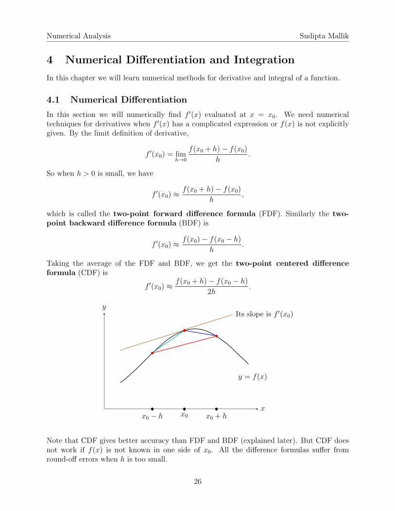
Taking the average of the FDF and BDF, we get the two-point centered differenceformula (CDF) is
f ′(x0) ≈f(x0 + h)− f(x0 − h)
2h.
x
y
y = f(x)
Its slope is f ′(x0)
x0 − h x0 x0 + h
Note that CDF gives better accuracy than FDF and BDF (explained later). But CDF doesnot work if f(x) is not known in one side of x0. All the difference formulas suffer fromround-off errors when h is too small.
26
Numerical Analysis Sudipta Mallik
Example. f(x) = x2ex. Approximate f ′(1) using the FDF, BDF, and CDF with h = 0.2.Solution.
Two-point FDF : f ′(1) ≈ f(1 + 0.2)− f(1)
0.2=
4.78− 2.71
0.2= 10.35
Two-point BDF : f ′(1) ≈ f(1)− f(1− 0.2)
0.2=
2.71− 1.42
0.2= 6.45
Two-point CDF : f ′(1) ≈ f(1 + 0.2)− f(1− 0.2)
2(0.2)=
4.78− 1.42
0.4= 8.4
Analytically we know f ′(1) = 3e. So the absolute errors are |10.35−3e| = 2.19, |6.45−3e| =1.7, and |8.4− 3e| = 0.24 respectively. So CDF gives the least error.
Errors in finite difference formulas: By the Taylor’s theorem on f about x0, we get
f(x) = f(x0) +f ′(x0)
1!(x− x0) +
f ′′(ξ)
2!(x− x0)2.
Plugging x = x0 + h, we get
f(x0 + h) = f(x0) +f ′(x0)
1!h+
f ′′(ξ1)
2!h2,
for some ξ1 ∈ (x0, x0 + h). Solving for f ′(x0), we get
f ′(x0) =f(x0 + h)− f(x0)
h− f ′′(ξ1)
2h.
The maximum error in FDF ish
2max
x∈(x0,x0+h)|f ′′(x)|.
So the error in FDF is O(h) (i.e., absolute error ≤ ch for some c > 0). It means small stepsize h results in more accurate derivative. We say FDF is first-order accurate. SimilarlyBDF is also first-order accurate with the maximum error
h
2max
x∈(x0−h,x0)|f ′′(x)|.
For CDF, note that
f(x0 + h) = f(x0) +f ′(x0)
1!h+
f ′′(x0)
2!h2 +
f ′′′(ξ1)
3!h3,
f(x0 − h) = f(x0)−f ′(x0)
1!h+
f ′′(x0)
2!h2 − f ′′′(ξ2)
3!h3,
for some ξ1 ∈ (x0, x0 + h) and ξ2 ∈ (x0 − h, x0). Subtracting we get,
27
Numerical Analysis Sudipta Mallik
f(x0 + h)− f(x0 − h) = 2f ′(x0)h+f ′′′(ξ1) + f ′′′(ξ2)
6h3
f(x0 + h)− f(x0 − h)
2h= f ′(x0) +
f ′′′(ξ1) + f ′′′(ξ2)
12h2
f ′(x0) =f(x0 + h)− f(x0 − h)
2h− f ′′′(ξ1) + f ′′′(ξ2)
12h2.
Assuming continuity of f ′′′ and using the IVT on f ′′′, we get
f ′′′(ξ) =f ′′′(ξ1) + f ′′′(ξ2)
2,
for some ξ ∈ (ξ2, ξ1) ⊂ (x0 − h, x0 + h). Thus
f ′(x0) =f(x0 + h)− f(x0 − h)
2h− f ′′′(ξ)
6h2.
The maximum error in CDF is
h2
6max
x∈(x0−h,x0+h)|f ′′′(x)|.
So the error in CDF is O(h2), i.e., CDF is second-order accurate which is better than first-order accurate as h2 << h for small h > 0.
Example. Consider f(x) = x2ex. Find the maximum error in approximating f ′(1) by theFDF, BDF, and CDF with h = 0.2.
Solution. f ′′(x) = (x2 + 4x+ 2)ex and f ′′′(x) = (x2 + 6x+ 6)ex are increasing functions forx > 0. So maxx∈(1,1.2) |f ′′(x)| = |f ′′(1.2)| = 27.3.
Maximum error in two-point FDF :0.2
2max
x∈(1,1.2)|f ′′(x)| = 0.1|f ′′(1.2)| = 2.73
Maximum error in two-point BDF :0.2
2max
x∈(0.8,1)|f ′′(x)| = 0.1|f ′′(1)| = 1.9
Maximum error in two-point CDF :(0.2)2
6max
x∈(0.8,1.2)|f ′′′(x)| = 0.04
6|f ′′′(1.2)| = 0.32
Derivative from Lagrange polynomial: If f is not explicitly given but we know (xi, f(xi))for i = 0, 1, . . . , n, then f is approximated by the Lagrange polynomial:
f(x) =n∑i=0
f(xi)Li(x) +f (n+1)(ξ(x))
(n+ 1)!
n∏i=0
(x− xi),
28
Numerical Analysis Sudipta Mallik
where ξ ∈ (x0, xn) and Li(x) =n∏j=0j 6=i
(x− xj)(xi − xj)
. Differentiating both sides and evaluating at
x = xj, we get(
steps skipped but note that ddx
∏ni=0(x− xi)
]x=xj
=∏n
i=0i 6=j
(xj − xi))
f ′(xj) =n∑i=0
f(xi)L′i(xj) +
f (n+1)(ξ)
(n+ 1)!
n∏i=0i 6=j
(xj − xi).
If the points x0, x1, . . . , xn are equally-spaced, i.e., xj = x0 + jh, then we get
f ′(xj) =n∑i=0
f(xi)L′i(xj) +
f (n+1)(ξ)
(n+ 1)!O(hn). (1)
It can be verified that two-point FDF and BDF are obtained from (1) using n = 1. Similarlyn = 2 gives the three-point FDF and BDF and two-point CDF whose errors are O(h2):
Three-point FDF : f ′(x0) ≈−3f(x0) + 4f(x0 + h)− f(x0 + 2h)
2h
Three-point BDF : f ′(x0) ≈3f(x0)− 4f(x0 − h) + f(x0 − 2h)
2h
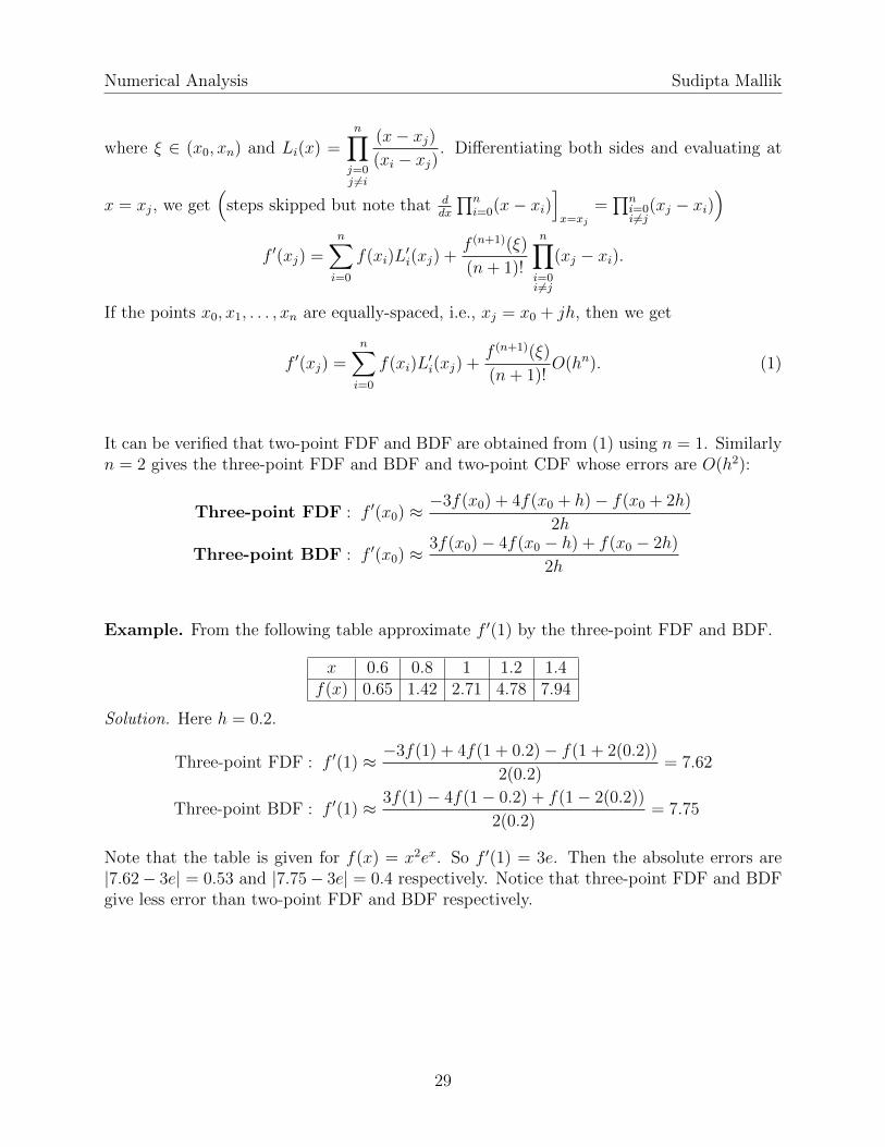
Example. From the following table approximate f ′(1) by the three-point FDF and BDF.
x 0.6 0.8 1 1.2 1.4f(x) 0.65 1.42 2.71 4.78 7.94
Solution. Here h = 0.2.
Three-point FDF : f ′(1) ≈ −3f(1) + 4f(1 + 0.2)− f(1 + 2(0.2))
2(0.2)= 7.62
Three-point BDF : f ′(1) ≈ 3f(1)− 4f(1− 0.2) + f(1− 2(0.2))
2(0.2)= 7.75
Note that the table is given for f(x) = x2ex. So f ′(1) = 3e. Then the absolute errors are|7.62− 3e| = 0.53 and |7.75− 3e| = 0.4 respectively. Notice that three-point FDF and BDFgive less error than two-point FDF and BDF respectively.
29
Numerical Analysis Sudipta Mallik
4.2 Elements of Numerical Integration
Sometimes it is hard to calculate a definite integral analytically. For example,
∫ 1
0
ex2
dx. To
approximate such an integral we break [a, b] into n subintervals [x0, x1], [x1, x2], . . . , [xn−1, xn]where xi = a + ih and h = (b − a)/n. Then we approximate the integral by a finite sumgiven by a quadrature rule (or, quadrature formula):∫ b
a
f(x) dx ≈n∑i=0
cif(xi).
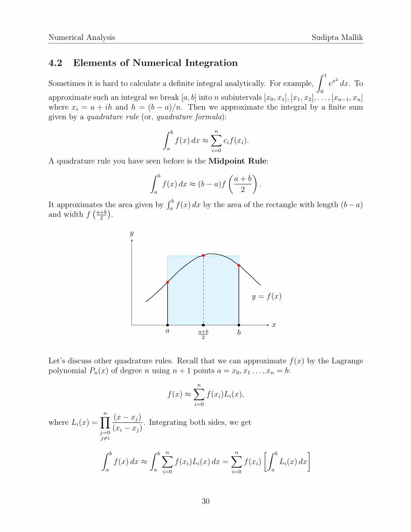
A quadrature rule you have seen before is the Midpoint Rule:∫ b
a
f(x) dx ≈ (b− a)f
(a+ b
2
).
It approximates the area given by∫ baf(x) dx by the area of the rectangle with length (b− a)
and width f(a+b2
).
x
y
y = f(x)
a ba+b2
Let’s discuss other quadrature rules. Recall that we can approximate f(x) by the Lagrangepolynomial Pn(x) of degree n using n+ 1 points a = x0, x1 . . . , xn = b:
f(x) ≈n∑i=0
f(xi)Li(x),
where Li(x) =n∏j=0j 6=i
(x− xj)(xi − xj)
. Integrating both sides, we get
∫ b
a
f(x) dx ≈∫ b
a
n∑i=0
f(xi)Li(x) dx =n∑i=0
f(xi)
[∫ b
a
Li(x) dx
]
30
Numerical Analysis Sudipta Mallik
=⇒∫ b
a
f(x) dx ≈n∑i=0
cif(xi),
where ci =∫ baLi(x) dx. We will discuss the quadrature rules given by n = 1 and 2.
For n = 1, we have n+ 1 = 2 points a = x0, x1 = b and then
f(x) ≈ P1(x) = f(x0)(x− x1)(x0 − x1)
+ f(x1)(x− x0)(x1 − x0)
= −f(a)(x− b)(b− a)
+ f(b)(x− a)
(b− a)
=⇒∫ b
a
f(x) dx ≈ − f(a)
b− a
∫ b
a
(x− b) dx+f(b)
b− a
∫ b
a
(x− a) dx
= − f(a)
b− a(x− b)2
2
]ba
+f(b)
b− a(x− a)2
2
]ba
= (b− a)
[f(a) + f(b)
2
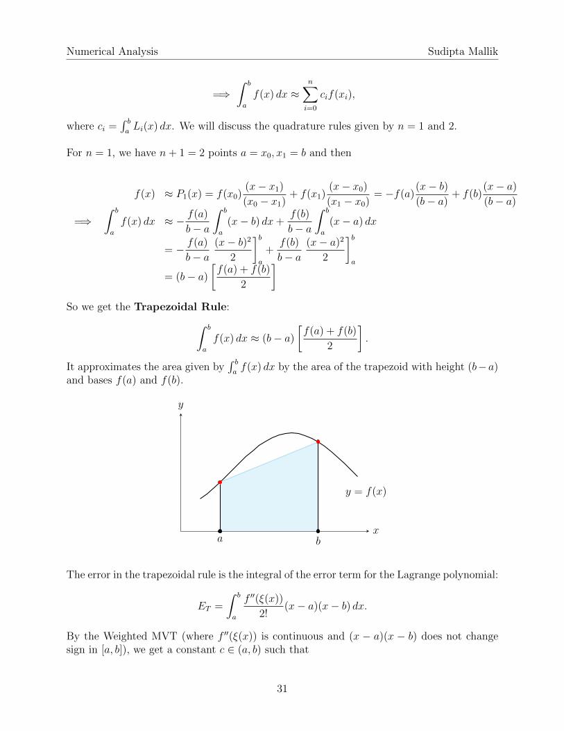
]So we get the Trapezoidal Rule:∫ b
a
f(x) dx ≈ (b− a)
[f(a) + f(b)
2
].
It approximates the area given by∫ baf(x) dx by the area of the trapezoid with height (b−a)
and bases f(a) and f(b).
x
y
y = f(x)
a b
The error in the trapezoidal rule is the integral of the error term for the Lagrange polynomial:
ET =
∫ b
a
f ′′(ξ(x))
2!(x− a)(x− b) dx.
By the Weighted MVT (where f ′′(ξ(x)) is continuous and (x − a)(x − b) does not changesign in [a, b]), we get a constant c ∈ (a, b) such that
31
Numerical Analysis Sudipta Mallik
ET =f ′′(c)
2
∫ b
a
(x− a)(x− b) dx = −f ′′(c)(b− a)3
12.
Similarly for n = 2, we have n+ 1 = 3 points a = x0, x1 = (a+ b)/2, x2 = b and then
f(x) ≈ P2(x) = f(x0)(x− x1)(x− x2)
(x0 − x1)(x0 − x2)+f(x1)
(x− x0)(x− x2)(x1 − x0)(x1 − x2)
+f(x1)(x− x0)(x− x1)
(x2 − x1)(x2 − x1).
Integrating we get the Simpson’s Rule:∫ b
a
f(x) dx ≈ (b− a)
6
[f(a) + 4f
(a+ b
2
)+ f(b)
]where the error in the Simpson’s Rule (obtained from the Taylor polynomial T3(x) of f aboutx = (a+ b)/2 with the error term) is
ES = −(b− a)5
90 · 25f (4)(c).
Note from ET that if f(x) is a polynomial of degree at most 1, then f ′′ = 0 and consequentlyET = 0. So the trapezoidal rule gives the exact integral. Similarly if f(x) is a polynomialof degree at most 3, then ES = 0 and consequently the Simpson’s rule gives the exact integral.
Example. Approximate
∫ 2
0
x3 dx by the Midpoint Rule, Trapezoidal Rule, Simpson’s Rule.
Solution. First of all let’s find the exact integral:∫ 2
0
x3 dx =x4
4
]20
= 4.
Midpoint :
∫ 2
0
x3 dx ≈ (b− a)f
(a+ b
2
)= (2− 0)
(0 + 2
2
)3
= 2
Trapezoidal :
∫ 2
0
x3 dx ≈ (b− a)
[f(a) + f(b)
2
]= (2− 0)
[0 + 23
2
]= 8
Simpson’s :
∫ 2
0
x3 dx ≈ (b− a)
6
[f(a) + 4f
(a+ b
2
)+ f(b)
]=
(2− 0)
6
[0 + 4 · 13 + 23
]= 4
The Simpson’s Rule gives the best approximation which turns out to be the exact integral.
Note that the error of the Midpoint Rule is always half of that of the Trapezoidal Rule.Because the Midpoint Rule is obtained by integrating the Taylor polynomial T1(x) of fabout x = (a+ b)/2 and integrating its remainder term, we can show that
EM =(b− a)3
24f ′′(c).
32
Numerical Analysis Sudipta Mallik
4.3 Composite Numerical Integration
Approximating
∫ b
a
f(x) dx by quadrature rules like trapezoidal, Simpson’s will give large
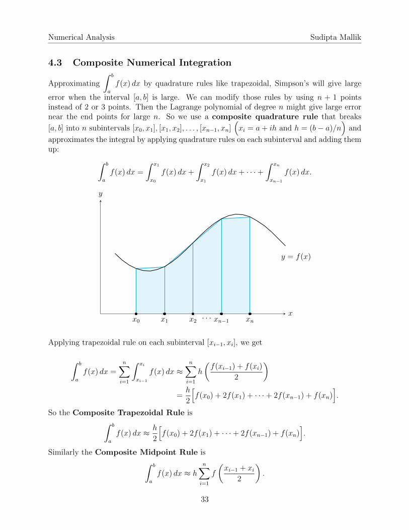
error when the interval [a, b] is large. We can modify those rules by using n + 1 pointsinstead of 2 or 3 points. Then the Lagrange polynomial of degree n might give large errornear the end points for large n. So we use a composite quadrature rule that breaks
[a, b] into n subintervals [x0, x1], [x1, x2], . . . , [xn−1, xn](xi = a+ ih and h = (b− a)/n
)and
approximates the integral by applying quadrature rules on each subinterval and adding themup: ∫ b
a
f(x) dx =
∫ x1
x0
f(x) dx+
∫ x2
x1
f(x) dx+ · · ·+∫ xn
xn−1
f(x) dx.
x
y
x0 x1 x2 xn−1· · · xn
y = f(x)
Applying trapezoidal rule on each subinterval [xi−1, xi], we get
∫ b
a
f(x) dx =n∑i=1
∫ xi
xi−1
f(x) dx ≈n∑i=1
h
(f(xi−1) + f(xi)
2
)=h
2
[f(x0) + 2f(x1) + · · ·+ 2f(xn−1) + f(xn)
].
So the Composite Trapezoidal Rule is∫ b
a
f(x) dx ≈ h
2
[f(x0) + 2f(x1) + · · ·+ 2f(xn−1) + f(xn)
].
Similarly the Composite Midpoint Rule is∫ b
a
f(x) dx ≈ h
n∑i=1
f
(xi−1 + xi
2
).
33
Numerical Analysis Sudipta Mallik
For the Composite Simpson’s Rule, we take even n and apply simple Simpson’s Rule tothe subintervals [x0, x2], [x2, x4], . . . , [xn−2, xn]:
∫ b
a
f(x) dx =
n/2∑i=1
∫ x2i
x2i−2
f(x) dx
≈n/2∑i=1
h
3
[f(x2i−2) + 4f(x2i−1) + f(x2i)
]=h
3
[(f(x0)+4f(x1)+f(x2)
)+
(f(x2)+4f(x3)+f(x4)
)+···+
(f(xn−2)+4f(xn−1)+f(xn)
)]=h
3
[f(x0)+f(xn)+4
(f(x1)+f(x3)+···+f(xn−1)
)+2
(f(x2)+f(x4)+···+f(xn−2)
)]
=h
3
f(x0) + f(xn) + 4
n/2∑i=1
f(x2i−1) + 2
(n−2)/2∑i=1
f(x2i)
Example. Approximate
∫ 2
0
ex dx using 4 subintervals in (a) Composite Trapezoidal Rule,
(b) Composite Midpoint Rule, (c) Composite Simpson’s Rule.
Solution. First of all let’s find the exact integral:
∫ 2
0
ex dx = ex]20
= e2 − 1 ≈ 6.389.
n = 4 =⇒ h = (2− 0)/4 = 0.5 and the 4 subintervals are [0, 0.5], [0.5, 1], [1, 1.5], [1.5, 2].
CTR :
∫ 2
0
ex dx ≈ 0.5
2
[e0 + 2e0.5 + 2e1 + 2e1.5 + e2
]= 6.52
CMR :
∫ 2
0
ex dx ≈ 0.5[e0.25 + e0.75 + e1.25 + e1.75
]= 6.32
CSR :
∫ 2
0
ex dx ≈ 0.5
3
[e0 + 4e0.5 + 2e1 + 4e1.5 + e2
]= 6.39
The error in the composite trapezoidal rule (using n subintervals) is given by
ETn = −n∑i=1
f ′′(ci)(xi − xi−1)3
12= −h
3
12
n∑i=1
f ′′(ci).
Assuming continuity of f ′′ on (a, b), by the IVT we can find c ∈ (a, b) such that
1
n
n∑i=1
f ′′(ci) = f ′′(c).
34
Numerical Analysis Sudipta Mallik
Thus∑n
i=1 f′′(ci) = nf ′′(c) and then
ETn = −nh3
12f ′′(c).
Note that n = (b− a)/h. Then the error for the composite trapezoidal rule becomes:
ETn = −(b− a)
12h2f ′′(c)
Similarly we get errors in the composite midpoint and Simpson’s rule:
EMn =(b− a)
24h2f ′′(c) ESn = −(b− a)
180h4f (4)(c)
Note that since errors are O(h2) and O(h4), small step sizes lead to more accurate integral.
Example. Find the step size h and the number of subintervals n required to approximate∫ 2
0
ex dx correct within 10−2 using (a) Composite Trapezoidal Rule, (b) Composite Midpoint
Rule, (c) Composite Simpson’s Rule.
Solution. Note f ′′(x) = f (4)(x) = ex which have the maximum absolute value e2 on [0, 2].
|ETn| =∣∣∣− (b− a)
12h2f ′′(c)
∣∣∣ ≤ (b− a)
12h2 ·max
[0,2]|f ′′(x)| = (2− 0)
12
(2− 0
n
)2
· e2 < 10−2
=⇒ n >√
200e2/3 = 22.19
Thus for the CTR we need n = 23 and h = (2− 0)/23 = 2/23 ≈ 0.087.
Similarly for the CMR we need n = 16 and h = (2− 0)/16 = 0.125,and for the CSR we need n = 4 and h = (2− 0)/4 = 0.5.
Algorithm Composite-Simpson’sInput: functionf , interval [a, b], an even number n of sunintervals
Output: an approximation of
∫ b
a
f(x) dx
set h = (b− a)/n;set I = f(a) + f(b);for i = 1 to n/2
I = I + 4 ∗ f(a+ (2i− 1) ∗ h)end forfor i = 1 to (n− 2)/2
I = I + 2 ∗ f(a+ 2i ∗ h)end forreturn I ∗ h/3
35
Numerical Analysis Sudipta Mallik
5 Differential Equations
In this chapter we numerically solve the following IVP (initial value problem):
dy
dt= f(t, y), a ≤ t ≤ b, y(a) = c (2)
Instead of finding y = y(t) on [a, b], we break [a, b] into n subintervals [t0, t1], [t1, t2], . . . , [tn−1, tn]and approximate y(ti), i = 0, 1, . . . , n. But if we need y(t), it can be approximated by theLagrange polynomial Pn using t0, t1, . . . , tn.
Before approximating a solution y = y(t), we must ask if (2) has a solution and it is uniqueon [a, b]. The answer is given by the Existence and Uniqueness Theorem:
Theorem 5.1. The IVP (2) has a unique solution y(t) on [a, b] if
1. f is continuous on D = {(t, y) | a ≤ t ≤ b, −∞ < y <∞}, and
2. f satisfies a Lipschitz condition on D with constant L:
|f(t, y1)− f(t, y2)| ≤ L|y1 − y2|, for all (t, y1), (t, y2) ∈ D.
When we approximate y(ti), i = 0, 1, . . . , n for the unique solution y(t), we might commitsome round-off errors. So we ask if the IVP (2) is well-posed:a small change in the problem (i.e., small change in f, c) gives a small change in the solution.
It can be proved that the IVP (2) is well-posed if f satisfies a Lipschitz condition on D. Alsonote that if |fy(t, y)| ≤ L on D, then f satisfies a Lipschitz condition on D with constant L.
5.1 Euler’s Method
We break [a, b] into n subintervals [t0, t1], [t1, t2], . . . , [tn−1, tn] where ti = a + ih and h =(b− a)/n. The Euler’s Method finds y0, y1, . . . , yn such that yi ≈ y(ti), i = 0, 1, . . . , n:
y0 = c
yi+1 = yi + hf(ti, yi), i = 0, 1, . . . , n− 1.
To justify the iterative formula, use Taylor’s theorem on y about t = ti:
y(t) = y(ti) + (t− ti)y′(ti) + (t−ti)22
y′′(ξi)
=⇒ y(ti+1) = y(ti) + (ti+1 − ti)y′(ti) + (ti+1−ti)22
y′′(ξi)
= y(ti) + hf(ti, y(ti)) + h2
2y′′(ξi)
=⇒ y(ti+1) ≈ yi + hf(ti, yi) =: yi+1
36
Numerical Analysis Sudipta Mallik
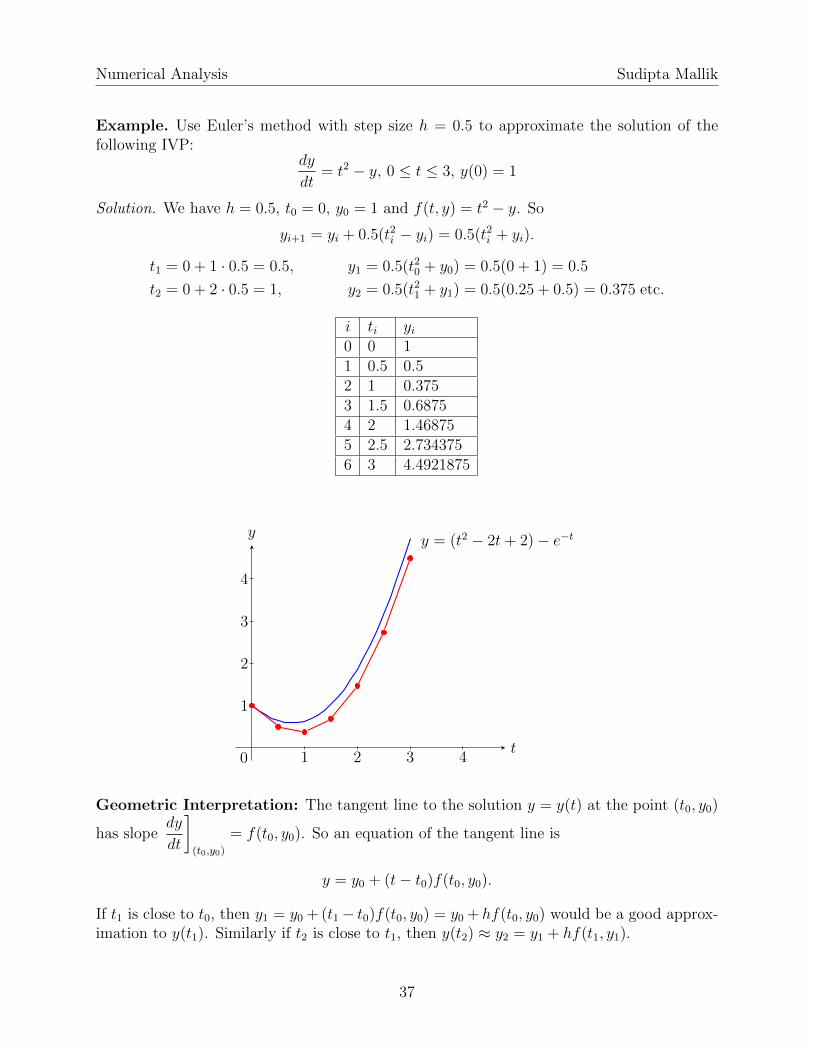
Example. Use Euler’s method with step size h = 0.5 to approximate the solution of thefollowing IVP:
dy
dt= t2 − y, 0 ≤ t ≤ 3, y(0) = 1
Solution. We have h = 0.5, t0 = 0, y0 = 1 and f(t, y) = t2 − y. So
yi+1 = yi + 0.5(t2i − yi) = 0.5(t2i + yi).
t1 = 0 + 1 · 0.5 = 0.5, y1 = 0.5(t20 + y0) = 0.5(0 + 1) = 0.5
t2 = 0 + 2 · 0.5 = 1, y2 = 0.5(t21 + y1) = 0.5(0.25 + 0.5) = 0.375 etc.
i ti yi0 0 11 0.5 0.52 1 0.3753 1.5 0.68754 2 1.468755 2.5 2.7343756 3 4.4921875
t
y
1 2 3 4
1
2
3
4
0
y = (t2 − 2t+ 2)− e−t
Geometric Interpretation: The tangent line to the solution y = y(t) at the point (t0, y0)
has slopedy
dt
](t0,y0)
= f(t0, y0). So an equation of the tangent line is
y = y0 + (t− t0)f(t0, y0).
If t1 is close to t0, then y1 = y0 + (t1− t0)f(t0, y0) = y0 + hf(t0, y0) would be a good approx-imation to y(t1). Similarly if t2 is close to t1, then y(t2) ≈ y2 = y1 + hf(t1, y1).
37
Numerical Analysis Sudipta Mallik
Maximum error: Suppose D = {(t, y) | a ≤ t ≤ b, −∞ < y < ∞} and f satisfies aLipschitz condition on D with constant L. Suppose y(t) is the unique solution to (2) where|y′′(t)| ≤ M for all t ∈ [a, b]. Then for the approximation yi of y(ti) by the Euler’s methodwith step size h, we have
|y(ti)− yi| ≤hM
2L
[−1 + eL(ti−a)
], i = 0, 1, . . . , n.
Proof. Use Taylor’s theorem and some inequality. See a standard textbook.
Example. Find the maximum error in approximating y(1) by y2 in the preceding example.Compare it with the actual absolute error using the solution y = (t2 − 2t+ 2)− e−t.
Solution. f(t, y) = t2 − y =⇒ |fy| = | − 1| ≤ 1 = L for all y. Thus f satisfies a Lipschitzcondition on D = (0, 3)× (−∞,∞) with the constant L = 1. Now
y = (t2 − 2t+ 2)− e−t =⇒ y′′ = 2− e−t.
Since y′′′ = e−t > 0, y′′ is an increasing function and then
|y′′| = |2− e−t| ≤ 2− e−3 = 1.95 = M for all t ∈ [0, 3]
Note h = 0.5, t2 = 1, and a = 0. Thus
|y(1)− y2| ≤hM
2L
[−1 + eL(t2−a)
]=
0.5 · 1.95
2 · 1[−1 + e1(1−0)
]= 0.83
Using the solution y = (t2 − 2t+ 2)− e−t, we get the actual absolute error
|y(1)− y2| = |(1− e−1)− 0.375| = 0.25.
38
Numerical Analysis Sudipta Mallik
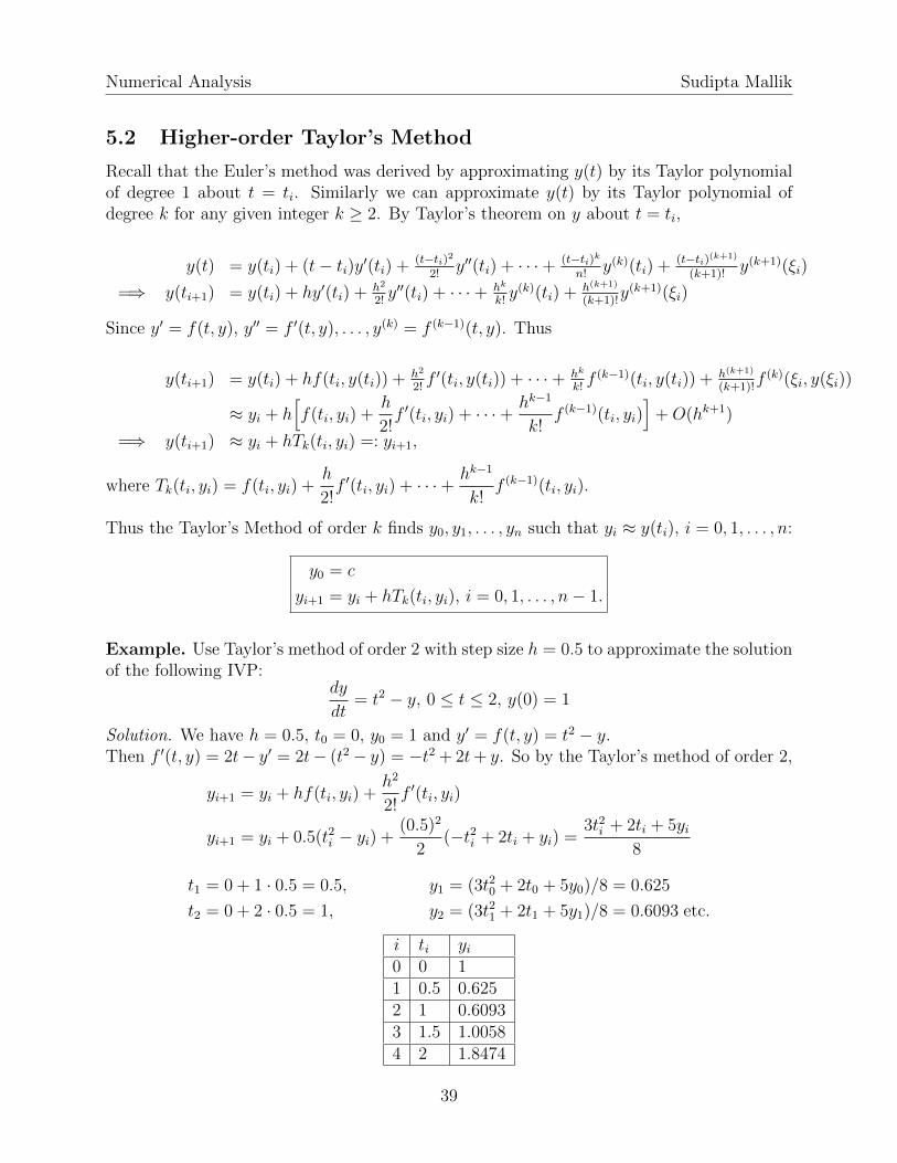
5.2 Higher-order Taylor’s Method
Recall that the Euler’s method was derived by approximating y(t) by its Taylor polynomialof degree 1 about t = ti. Similarly we can approximate y(t) by its Taylor polynomial ofdegree k for any given integer k ≥ 2. By Taylor’s theorem on y about t = ti,
y(t) = y(ti) + (t− ti)y′(ti) + (t−ti)22!
y′′(ti) + · · ·+ (t−ti)kn!
y(k)(ti) + (t−ti)(k+1)
(k+1)!y(k+1)(ξi)
=⇒ y(ti+1) = y(ti) + hy′(ti) + h2
2!y′′(ti) + · · ·+ hk
k!y(k)(ti) + h(k+1)
(k+1)!y(k+1)(ξi)
Since y′ = f(t, y), y′′ = f ′(t, y), . . . , y(k) = f (k−1)(t, y). Thus
y(ti+1) = y(ti) + hf(ti, y(ti)) + h2
2!f ′(ti, y(ti)) + · · ·+ hk
k!f (k−1)(ti, y(ti)) + h(k+1)
(k+1)!f (k)(ξi, y(ξi))
≈ yi + h[f(ti, yi) +
h
2!f ′(ti, yi) + · · ·+ hk−1
k!f (k−1)(ti, yi)
]+O(hk+1)
=⇒ y(ti+1) ≈ yi + hTk(ti, yi) =: yi+1,
where Tk(ti, yi) = f(ti, yi) +h
2!f ′(ti, yi) + · · ·+ hk−1
k!f (k−1)(ti, yi).
Thus the Taylor’s Method of order k finds y0, y1, . . . , yn such that yi ≈ y(ti), i = 0, 1, . . . , n:
y0 = c
yi+1 = yi + hTk(ti, yi), i = 0, 1, . . . , n− 1.
Example. Use Taylor’s method of order 2 with step size h = 0.5 to approximate the solutionof the following IVP:
dy
dt= t2 − y, 0 ≤ t ≤ 2, y(0) = 1
Solution. We have h = 0.5, t0 = 0, y0 = 1 and y′ = f(t, y) = t2 − y.Then f ′(t, y) = 2t− y′ = 2t− (t2− y) = −t2 + 2t+ y. So by the Taylor’s method of order 2,
yi+1 = yi + hf(ti, yi) +h2
2!f ′(ti, yi)
yi+1 = yi + 0.5(t2i − yi) +(0.5)2
2(−t2i + 2ti + yi) =
3t2i + 2ti + 5yi8
t1 = 0 + 1 · 0.5 = 0.5, y1 = (3t20 + 2t0 + 5y0)/8 = 0.625
t2 = 0 + 2 · 0.5 = 1, y2 = (3t21 + 2t1 + 5y1)/8 = 0.6093 etc.
i ti yi0 0 11 0.5 0.6252 1 0.60933 1.5 1.00584 2 1.8474
39
Numerical Analysis Sudipta Mallik
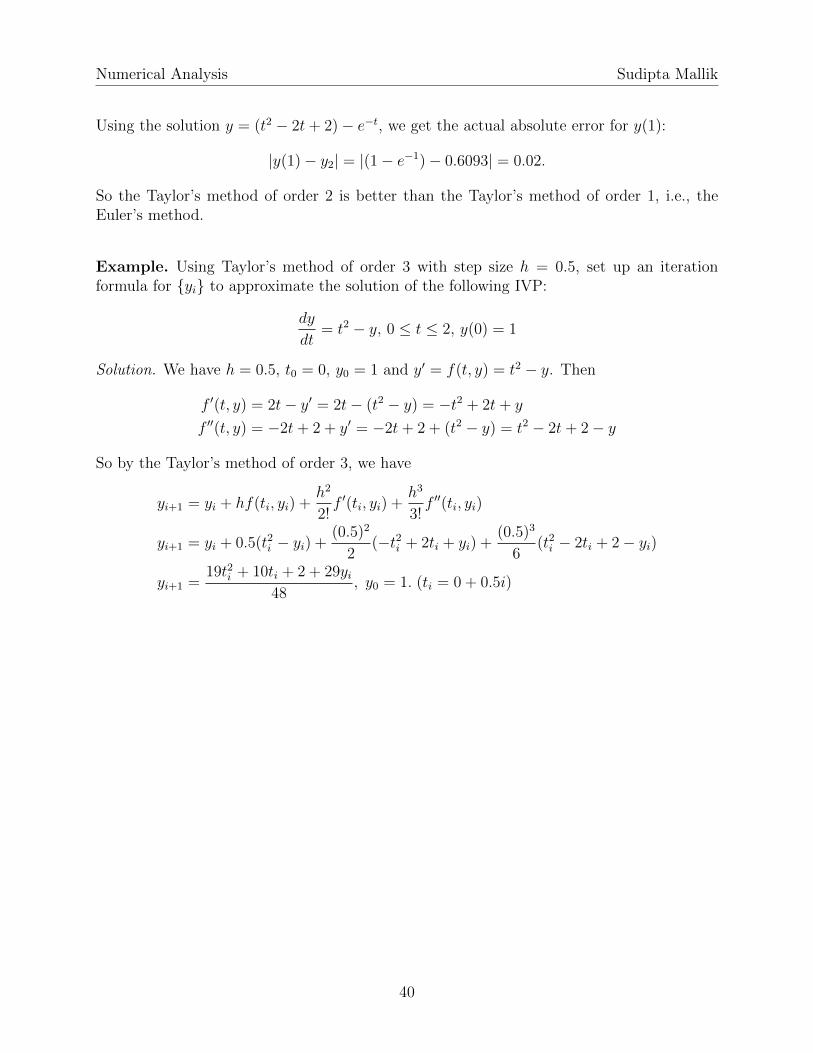
Using the solution y = (t2 − 2t+ 2)− e−t, we get the actual absolute error for y(1):
|y(1)− y2| = |(1− e−1)− 0.6093| = 0.02.
So the Taylor’s method of order 2 is better than the Taylor’s method of order 1, i.e., theEuler’s method.
Example. Using Taylor’s method of order 3 with step size h = 0.5, set up an iterationformula for {yi} to approximate the solution of the following IVP:
dy
dt= t2 − y, 0 ≤ t ≤ 2, y(0) = 1
Solution. We have h = 0.5, t0 = 0, y0 = 1 and y′ = f(t, y) = t2 − y. Then
f ′(t, y) = 2t− y′ = 2t− (t2 − y) = −t2 + 2t+ y
f ′′(t, y) = −2t+ 2 + y′ = −2t+ 2 + (t2 − y) = t2 − 2t+ 2− y
So by the Taylor’s method of order 3, we have
yi+1 = yi + hf(ti, yi) +h2
2!f ′(ti, yi) +
h3
3!f ′′(ti, yi)
yi+1 = yi + 0.5(t2i − yi) +(0.5)2
2(−t2i + 2ti + yi) +
(0.5)3
6(t2i − 2ti + 2− yi)
yi+1 =19t2i + 10ti + 2 + 29yi
48, y0 = 1. (ti = 0 + 0.5i)
40
Numerical Analysis Sudipta Mallik
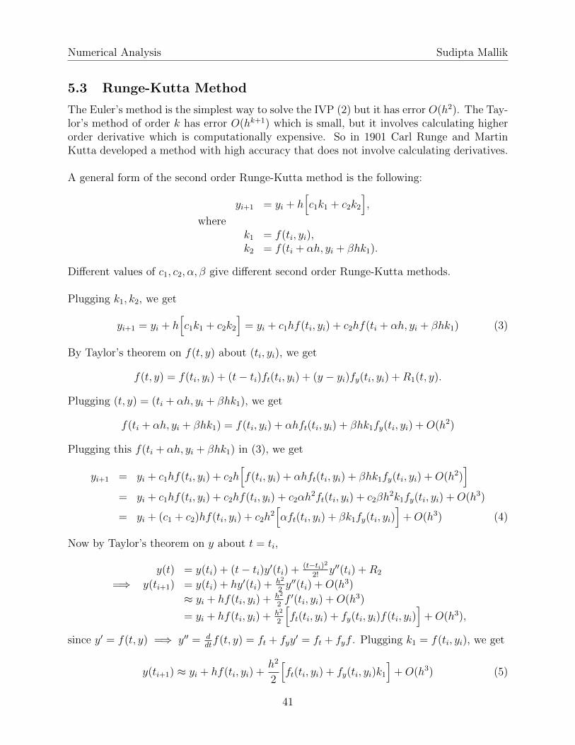
5.3 Runge-Kutta Method
The Euler’s method is the simplest way to solve the IVP (2) but it has error O(h2). The Tay-lor’s method of order k has error O(hk+1) which is small, but it involves calculating higherorder derivative which is computationally expensive. So in 1901 Carl Runge and MartinKutta developed a method with high accuracy that does not involve calculating derivatives.
A general form of the second order Runge-Kutta method is the following:
yi+1 = yi + h[c1k1 + c2k2
],
wherek1 = f(ti, yi),k2 = f(ti + αh, yi + βhk1).
Different values of c1, c2, α, β give different second order Runge-Kutta methods.
Plugging k1, k2, we get
yi+1 = yi + h[c1k1 + c2k2
]= yi + c1hf(ti, yi) + c2hf(ti + αh, yi + βhk1) (3)
By Taylor’s theorem on f(t, y) about (ti, yi), we get
f(t, y) = f(ti, yi) + (t− ti)ft(ti, yi) + (y − yi)fy(ti, yi) +R1(t, y).
Plugging (t, y) = (ti + αh, yi + βhk1), we get
f(ti + αh, yi + βhk1) = f(ti, yi) + αhft(ti, yi) + βhk1fy(ti, yi) +O(h2)
Plugging this f(ti + αh, yi + βhk1) in (3), we get
yi+1 = yi + c1hf(ti, yi) + c2h[f(ti, yi) + αhft(ti, yi) + βhk1fy(ti, yi) +O(h2)
]= yi + c1hf(ti, yi) + c2hf(ti, yi) + c2αh
2ft(ti, yi) + c2βh2k1fy(ti, yi) +O(h3)
= yi + (c1 + c2)hf(ti, yi) + c2h2[αft(ti, yi) + βk1fy(ti, yi)
]+O(h3) (4)
Now by Taylor’s theorem on y about t = ti,
y(t) = y(ti) + (t− ti)y′(ti) + (t−ti)22!
y′′(ti) +R2
=⇒ y(ti+1) = y(ti) + hy′(ti) + h2
2y′′(ti) +O(h3)
≈ yi + hf(ti, yi) + h2
2f ′(ti, yi) +O(h3)
= yi + hf(ti, yi) + h2
2
[ft(ti, yi) + fy(ti, yi)f(ti, yi)
]+O(h3),
since y′ = f(t, y) =⇒ y′′ = ddtf(t, y) = ft + fyy
′ = ft + fyf . Plugging k1 = f(ti, yi), we get
y(ti+1) ≈ yi + hf(ti, yi) +h2
2
[ft(ti, yi) + fy(ti, yi)k1
]+O(h3) (5)
41
Numerical Analysis Sudipta Mallik
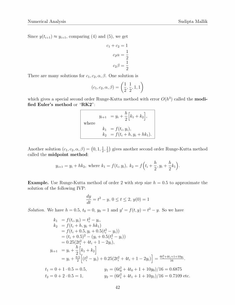
Since y(ti+1) ≈ yi+1, comparing (4) and (5), we get
c1 + c2 = 1
c2α =1
2
c2β =1
2
There are many solutions for c1, c2, α, β. One solution is
(c1, c2, α, β) =
(1
2,1
2, 1, 1
)which gives a special second order Runge-Kutta method with error O(h3) called the modi-fied Euler’s method or “RK2”:
yi+1 = yi +h
2
[k1 + k2
],
wherek1 = f(ti, yi),k2 = f(ti + h, yi + hk1).
Another solution (c1, c2, α, β) =(0, 1, 1
2, 12
)gives another second order Runge-Kutta method
called the midpoint method:
yi+1 = yi + hk2, where k1 = f(ti, yi), k2 = f(ti +
h
2, yi +
h
2k1
).
Example. Use Runge-Kutta method of order 2 with step size h = 0.5 to approximate thesolution of the following IVP:
dy
dt= t2 − y, 0 ≤ t ≤ 2, y(0) = 1
Solution. We have h = 0.5, t0 = 0, y0 = 1 and y′ = f(t, y) = t2 − y. So we have
k1 = f(ti, yi) = t2i − yi,k2 = f(ti + h, yi + hk1)
= f(ti + 0.5, yi + 0.5(t2i − yi))= (ti + 0.5)2 − (yi + 0.5(t2i − yi))= 0.25(2t2i + 4ti + 1− 2yi),
yi+1 = yi +h
2
[k1 + k2
]= yi + 0.5
2
[(t2i − yi) + 0.25(2t2i + 4ti + 1− 2yi)
]=
6t2i+4ti+1+10yi16
.
t1 = 0 + 1 · 0.5 = 0.5, y1 = (6t20 + 4t0 + 1 + 10y0)/16 = 0.6875
t2 = 0 + 2 · 0.5 = 1, y2 = (6t21 + 4t1 + 1 + 10y1)/16 = 0.7109 etc.
42
Numerical Analysis Sudipta Mallik
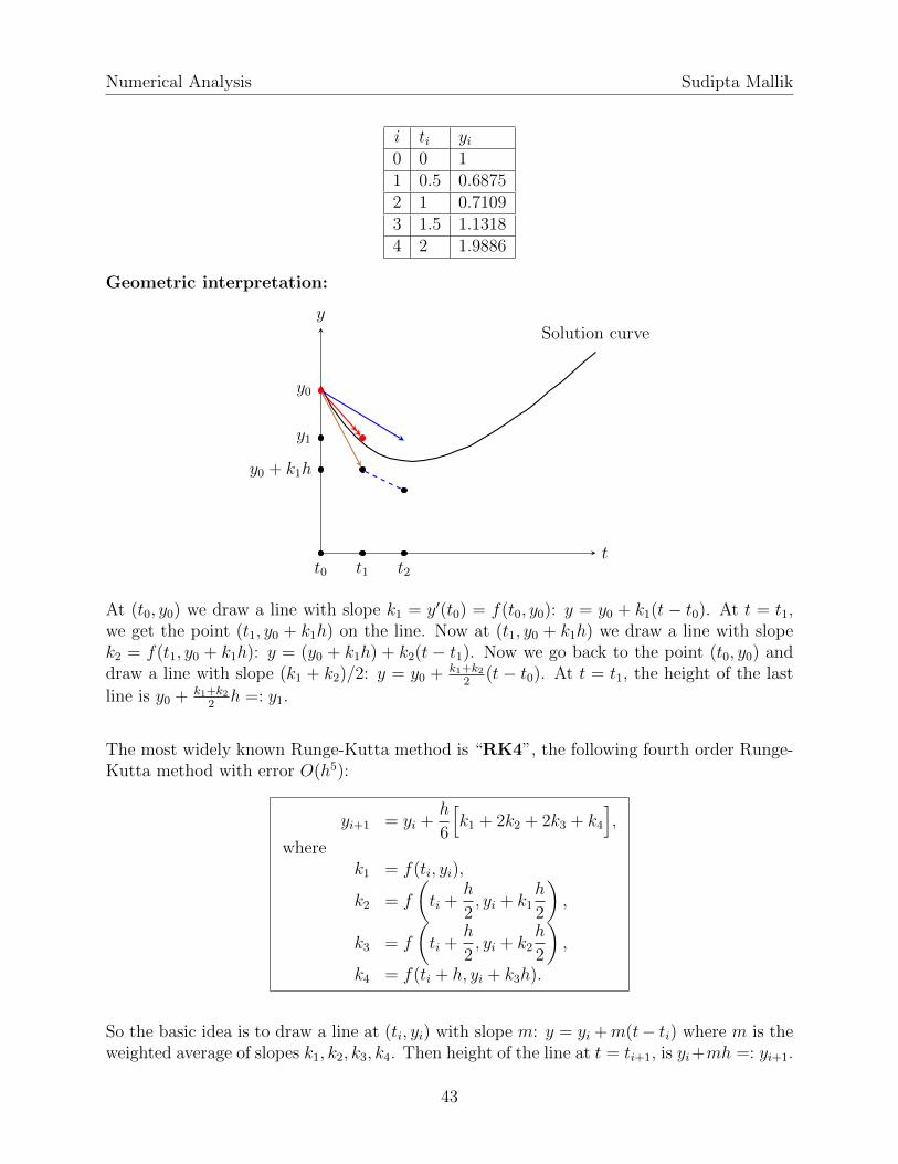
i ti yi0 0 11 0.5 0.68752 1 0.71093 1.5 1.13184 2 1.9886
Geometric interpretation:
t
ySolution curve
y0
y1
t0 t1 t2
y0 + k1h
At (t0, y0) we draw a line with slope k1 = y′(t0) = f(t0, y0): y = y0 + k1(t − t0). At t = t1,we get the point (t1, y0 + k1h) on the line. Now at (t1, y0 + k1h) we draw a line with slopek2 = f(t1, y0 + k1h): y = (y0 + k1h) + k2(t − t1). Now we go back to the point (t0, y0) anddraw a line with slope (k1 + k2)/2: y = y0 + k1+k2
2(t − t0). At t = t1, the height of the last
line is y0 + k1+k22h =: y1.
The most widely known Runge-Kutta method is “RK4”, the following fourth order Runge-Kutta method with error O(h5):
yi+1 = yi +h
6
[k1 + 2k2 + 2k3 + k4
],
wherek1 = f(ti, yi),
k2 = f
(ti +
h
2, yi + k1
h
2
),
k3 = f
(ti +
h
2, yi + k2
h
2
),
k4 = f(ti + h, yi + k3h).
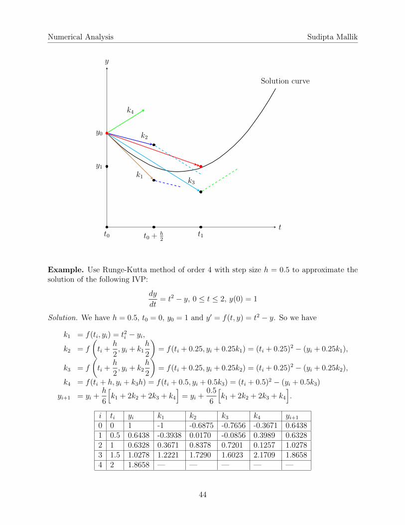
So the basic idea is to draw a line at (ti, yi) with slope m: y = yi +m(t− ti) where m is theweighted average of slopes k1, k2, k3, k4. Then height of the line at t = ti+1, is yi+mh =: yi+1.
43
Numerical Analysis Sudipta Mallik
t
y
Solution curve
y0
y1k1
k3
k2
k4
t0 t0 + h2
t1
Example. Use Runge-Kutta method of order 4 with step size h = 0.5 to approximate thesolution of the following IVP:
dy
dt= t2 − y, 0 ≤ t ≤ 2, y(0) = 1
Solution. We have h = 0.5, t0 = 0, y0 = 1 and y′ = f(t, y) = t2 − y. So we have
k1 = f(ti, yi) = t2i − yi,
k2 = f
(ti +
h
2, yi + k1
h
2
)= f(ti + 0.25, yi + 0.25k1) = (ti + 0.25)2 − (yi + 0.25k1),
k3 = f
(ti +
h
2, yi + k2
h
2
)= f(ti + 0.25, yi + 0.25k2) = (ti + 0.25)2 − (yi + 0.25k2),
k4 = f(ti + h, yi + k3h) = f(ti + 0.5, yi + 0.5k3) = (ti + 0.5)2 − (yi + 0.5k3)
yi+1 = yi +h
6
[k1 + 2k2 + 2k3 + k4
]= yi +
0.5
6
[k1 + 2k2 + 2k3 + k4
].
i ti yi k1 k2 k3 k4 yi+1
0 0 1 -1 -0.6875 -0.7656 -0.3671 0.64381 0.5 0.6438 -0.3938 0.0170 -0.0856 0.3989 0.63282 1 0.6328 0.3671 0.8378 0.7201 0.1257 1.02783 1.5 1.0278 1.2221 1.7290 1.6023 2.1709 1.86584 2 1.8658 — — — — —
44
Numerical Analysis Sudipta Mallik
6 Linear Algebra
In this chapter we will learn introductory linear algebra and numerical methods for solvingsystem of linear equations and finding eigenvalues of a matrix.
6.1 Introduction to Linear Algebra
Matrix: An m× n matrix A is an m-by-n array of scalars of the form
A =
a11 a12 · · · a1na21 a22 · · · a2n...
......
am1 am2 · · · amn
.The order (or size) of A is m× n (read as m by n). It means A has m rows and n columns.The (i, j)-entry of A = [ai,j] is ai,j.
Example. A =
[1 2 0−3 0 −1
]is a 2× 3 real matrix. The (2, 3)-entry of A is −1.
The identity matrix of order n, denoted by In, is the n×n diagonal matrix whose diagonal
entries are 1. Example. I3 =
1 0 00 1 00 0 1
is the 3× 3 identity matrix.
An n×1 matrix is called a column matrix or n-dimensional (column) vector. It is denoted by
−→x . Example. −→x =
10−2
is a 3-dimensional vector which represents the position vector
of the point (1, 0,−2) in R3.
Now we will learn some operations on matrices.
• Norm: We will use only two norms of a vector −→x =
x1...xn
:
1. l2 norm (Euclidean norm): ||−→x ||2 =√x21 + · · ·+ x2n
2. l∞ norm: ||−→x ||∞ = max1≤i≤n
|xi|
For the above −→x , ||−→x ||2 =√
5 and ||−→x ||∞ = 2. Note that ||−→x ||∞ ≤ ||−→x ||2 for all −→x .
45
Numerical Analysis Sudipta Mallik
• Transpose: The transpose of an m × n matrix A, denoted by AT , is an n × m matrixwhose columns are corresponding rows of A, i.e., (AT )ij = Aji.
Example. If A =
[1 2 0−3 0 −1
], then AT =
1 −32 00 −1
.
• Scalar Multiplication: Let A be a matrix and c be a scalar. The scalar multiple, denotedby cA, is the matrix whose entries are c times the corresponding entries of A.
Example. If A =
[1 2 0−3 0 −1
], then −2A =
[−2 −4 0
6 0 2
].
• Sum: If A and B are m × n matrices, then the sum A + B is the m × n matrix whoseentries are the sum of the corresponding entries of A and B, i.e., (A+B)ij = Aij +Bij.
Example. If A =
[1 2 0−3 0 −1
]and B =
[0 −2 03 0 2
], then A+B =
[1 0 00 0 1
].
Exercise. Find 2A−B.
• Multiplication:
1. Matrix-vector multiplication: If A is an m × n matrix and −→x is an n-dimensionalvector, then their product A−→x is an n-dimensional vector whose (i, 1)-entry is ai1x1 +ai2x2 + · · ·+ aimxn, the dot product of the row i of A and −→x . Note that
A−→x =
a11x1 + a12x2 + · · ·+ a1nxna21x1 + a22x2 + · · ·+ a2nxn
...am1x1 + am2x2 + · · ·+ amnxn
= x1
a11a21...am1
+x2
a12a22...am2
+· · ·+xn
a1na2n...
amn
.
Example. If A =
[1 2 0−3 0 −1
]and −→x =
1−1
0
, then A−→x =
[−1−3
]which is a
linear combination of first and second columns of A with weights 1 and −1 respectively.
2. Matrix-matrix multiplication: If A is an m× n matrix and B is an n× p matrix, thentheir product AB is an m× p matrix whose (i, j)-entry is the dot product the row i ofA and the column j of B.
(AB)ij = ai1b1j + ai2b2j + · · ·+ aimbmj
Note that column i of AB is A(column i of B). Also note AB 6= BA in general.
Example. If A =
[1 2 20 0 2
]and B =
2 −20 01 1
, then AB =
[4 02 2
].
46
Numerical Analysis Sudipta Mallik
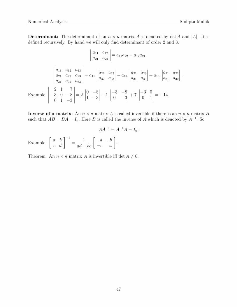
Determinant: The determinant of an n × n matrix A is denoted by detA and |A|. It isdefined recursively. By hand we will only find determinant of order 2 and 3.
a11 a12a21 a22
= a11a22 − a12a21.
a11 a12 a13a21 a22 a23a31 a32 a33
= a11
∣∣∣∣a22 a23a32 a33
∣∣∣∣− a12 ∣∣∣∣a21 a23a31 a33
∣∣∣∣+ a13
∣∣∣∣a21 a22a31 a32
∣∣∣∣ .Example.
2 1 7−3 0 −8
0 1 −3= 2
∣∣∣∣0 −81 −3
∣∣∣∣− 1
∣∣∣∣−3 −80 −3
∣∣∣∣+ 7
∣∣∣∣−3 00 1
∣∣∣∣ = −14.
Inverse of a matrix: An n× n matrix A is called invertible if there is an n× n matrix Bsuch that AB = BA = In. Here B is called the inverse of A which is denoted by A−1. So
AA−1 = A−1A = In.
Example.
[a bc d
]−1=
1
ad− bc
[d −b−c a
].
Theorem. An n× n matrix A is invertible iff detA 6= 0.
47
Numerical Analysis Sudipta Mallik
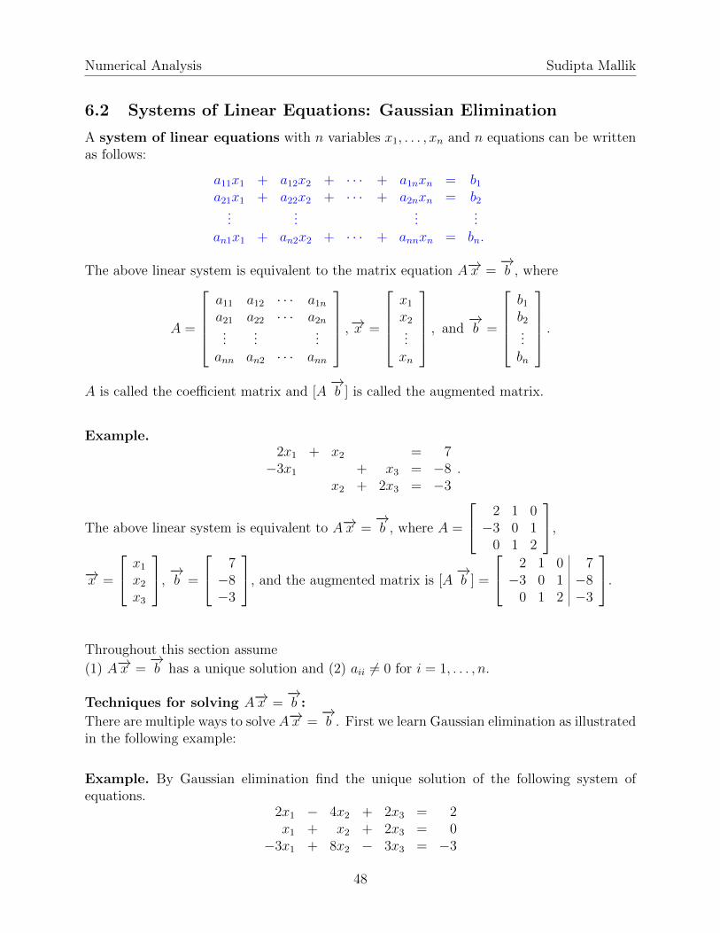
6.2 Systems of Linear Equations: Gaussian Elimination
A system of linear equations with n variables x1, . . . , xn and n equations can be writtenas follows:
a11x1 + a12x2 + · · · + a1nxn = b1a21x1 + a22x2 + · · · + a2nxn = b2
......
......
an1x1 + an2x2 + · · · + annxn = bn.
The above linear system is equivalent to the matrix equation A−→x =−→b , where
A =
a11 a12 · · · a1na21 a22 · · · a2n...
......
ann an2 · · · ann
,−→x =
x1x2...xn
, and−→b =
b1b2...bn
.A is called the coefficient matrix and [A
−→b ] is called the augmented matrix.
Example.2x1 + x2 = 7−3x1 + x3 = −8
x2 + 2x3 = −3.
The above linear system is equivalent to A−→x =−→b , where A =
2 1 0−3 0 1
0 1 2
,
−→x =
x1x2x3
,−→b =
7−8−3
, and the augmented matrix is [A−→b ] =
2 1 0 7−3 0 1 −8
0 1 2 −3
.
Throughout this section assume
(1) A−→x =−→b has a unique solution and (2) aii 6= 0 for i = 1, . . . , n.
Techniques for solving A−→x =−→b :
There are multiple ways to solve A−→x =−→b . First we learn Gaussian elimination as illustrated
in the following example:
Example. By Gaussian elimination find the unique solution of the following system ofequations.
2x1 − 4x2 + 2x3 = 2x1 + x2 + 2x3 = 0
−3x1 + 8x2 − 3x3 = −3
48
Numerical Analysis Sudipta Mallik
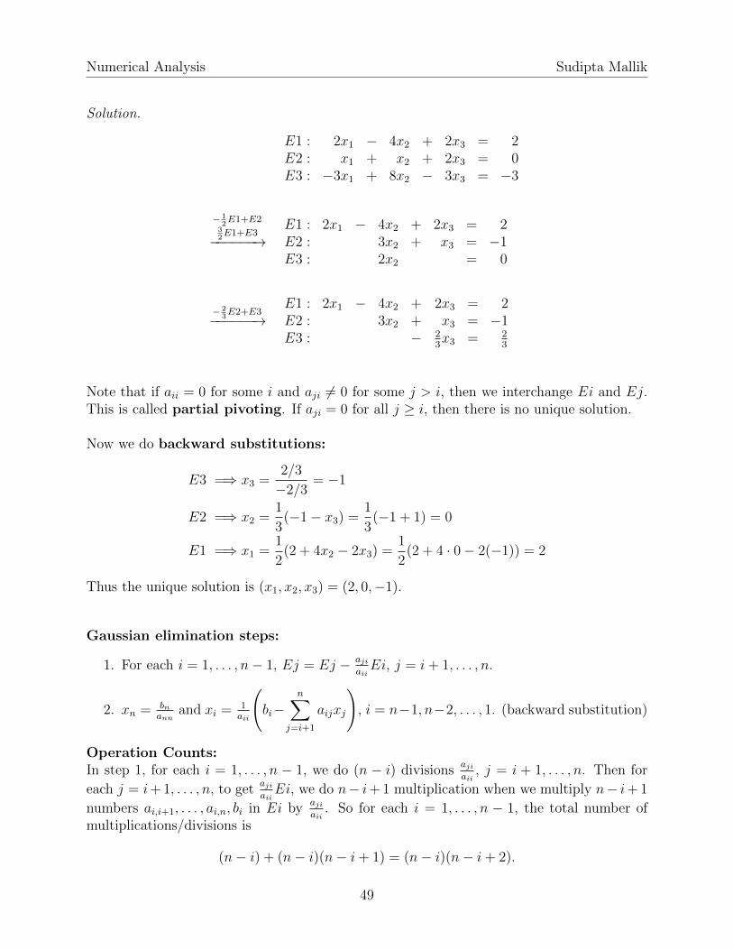
Solution.
E1 : 2x1 − 4x2 + 2x3 = 2E2 : x1 + x2 + 2x3 = 0E3 : −3x1 + 8x2 − 3x3 = −3
− 12E1+E2
32E1+E3−−−−−−→
E1 : 2x1 − 4x2 + 2x3 = 2E2 : 3x2 + x3 = −1E3 : 2x2 = 0
− 23E2+E3
−−−−−−→E1 : 2x1 − 4x2 + 2x3 = 2E2 : 3x2 + x3 = −1E3 : − 2
3x3 = 2
3
Note that if aii = 0 for some i and aji 6= 0 for some j > i, then we interchange Ei and Ej.This is called partial pivoting. If aji = 0 for all j ≥ i, then there is no unique solution.
Now we do backward substitutions:
E3 =⇒ x3 =2/3
−2/3= −1
E2 =⇒ x2 =1
3(−1− x3) =
1
3(−1 + 1) = 0
E1 =⇒ x1 =1
2(2 + 4x2 − 2x3) =
1
2(2 + 4 · 0− 2(−1)) = 2
Thus the unique solution is (x1, x2, x3) = (2, 0,−1).
Gaussian elimination steps:
1. For each i = 1, . . . , n− 1, Ej = Ej − ajiaiiEi, j = i+ 1, . . . , n.
2. xn = bnann
and xi = 1aii
(bi−
n∑j=i+1
aijxj
), i = n−1, n−2, . . . , 1. (backward substitution)
Operation Counts:In step 1, for each i = 1, . . . , n − 1, we do (n − i) divisions
ajiaii
, j = i + 1, . . . , n. Then for
each j = i+ 1, . . . , n, to getajiaiiEi, we do n− i+ 1 multiplication when we multiply n− i+ 1
numbers ai,i+1, . . . , ai,n, bi in Ei byajiaii
. So for each i = 1, . . . , n − 1, the total number ofmultiplications/divisions is
(n− i) + (n− i)(n− i+ 1) = (n− i)(n− i+ 2).
49
Numerical Analysis Sudipta Mallik
For a fixed i = 1, . . . , n − 1, we do (n − i + 1) subtraction for Ej = Ej − ajiaiiEi for each
j = i+ 1, . . . , n, i.e., total (n− i)(n− i+ 1) subtractions.
So the total number of multiplications/divisions is
n−1∑i=1
(n− i)(n− i+ 2) =2n3 + 3n2 − 5n
6.
The total number of subtractions is
n−1∑i=1
(n− i)(n− i+ 1) =n3 − n
3.
Note that in a computer the time for a multiplication/division is greater than that of an
addition/subtraction. So the total number of operations in step 1 is2n3 + 3n2 − 5n
6+
n3 − n3
=4n3 + 3n2 − 7n
6which is O(n3). Similarly we can show the total number of
operations in step 2 isn2 + n
2+n2 − n
2= n2. Thus total number of operations in Gaussian
elimination is4n3 + 3n2 − 7n
6+ n2 =
4n3 + 9n2 − 7n
6which is O(n3).
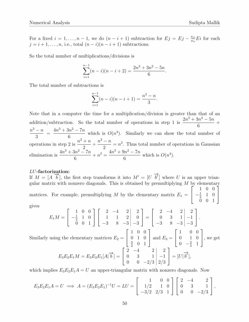
LU-factorization:If M = [A
−→b ], the first step transforms it into M ′ = [U
−→b′ ] where U is an upper trian-
gular matrix with nonzero diagonals. This is obtained by premultiplying M by elementary
matrices. For example, premultiplying M by the elementary matrix E1 =
1 0 0−1
21 0
0 0 1
gives
E1M =
1 0 0−1
21 0
0 0 1
2 −4 2 21 1 2 0−3 8 −3 −3
=
2 −4 2 20 3 1 −1−3 8 −3 −3
.Similarly using the elementary matrices E2 =
1 0 00 1 032
0 1
and E3 =
1 0 00 1 00 −2
31
, we get
E3E2E1M = E3E2E1[A|−→b ] =
2 −4 2 20 3 1 −10 0 −2/3 2/3
= [U |−→b′ ],
which implies E3E2E1A = U an upper-triangular matrix with nonzero diagonals. Now
E3E2E1A = U =⇒ A = (E3E2E1)−1U = LU =
1 0 01/2 1 0−3/2 2/3 1
2 −4 20 3 10 0 −2/3
,50
Numerical Analysis Sudipta Mallik
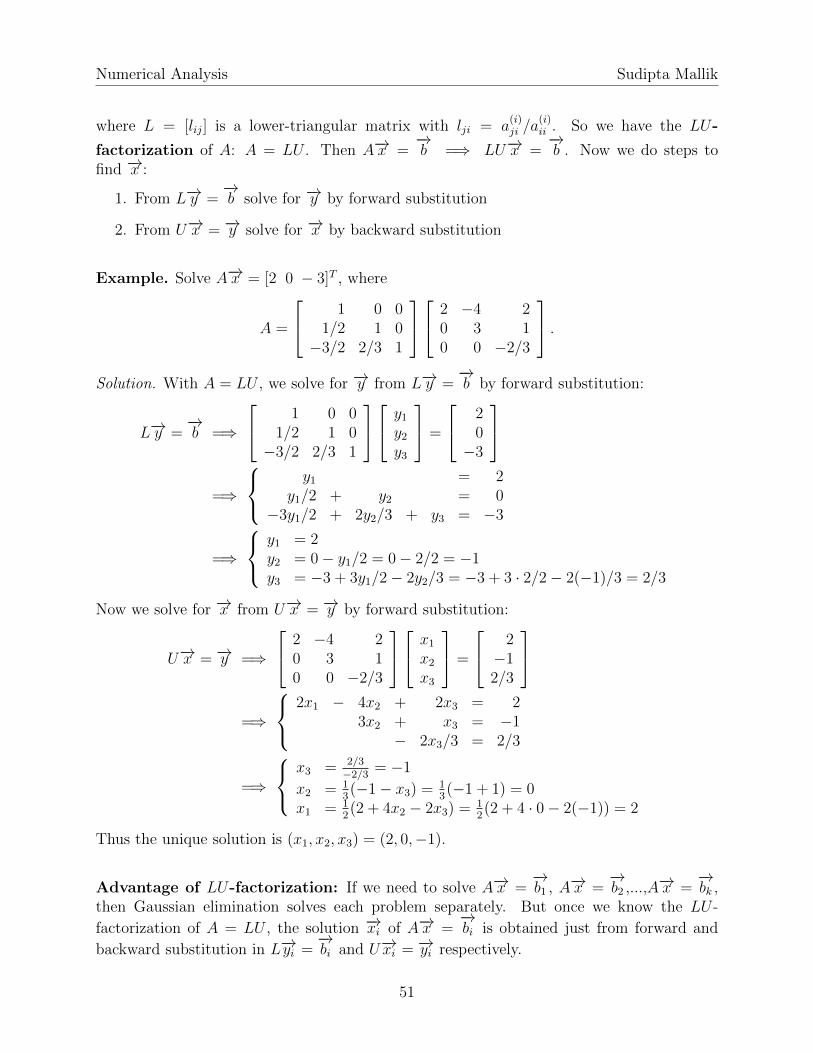
where L = [lij] is a lower-triangular matrix with lji = a(i)ji /a
(i)ii . So we have the LU-
factorization of A: A = LU . Then A−→x =−→b =⇒ LU−→x =
−→b . Now we do steps to
find −→x :
1. From L−→y =−→b solve for −→y by forward substitution
2. From U−→x = −→y solve for −→x by backward substitution
Example. Solve A−→x = [2 0 − 3]T , where
A =
1 0 01/2 1 0−3/2 2/3 1
2 −4 20 3 10 0 −2/3
.Solution. With A = LU , we solve for −→y from L−→y =
−→b by forward substitution:
L−→y =−→b =⇒
1 0 01/2 1 0−3/2 2/3 1
y1y2y3
=
20−3
=⇒
y1 = 2
y1/2 + y2 = 0−3y1/2 + 2y2/3 + y3 = −3
=⇒
y1 = 2y2 = 0− y1/2 = 0− 2/2 = −1y3 = −3 + 3y1/2− 2y2/3 = −3 + 3 · 2/2− 2(−1)/3 = 2/3
Now we solve for −→x from U−→x = −→y by forward substitution:
U−→x = −→y =⇒
2 −4 20 3 10 0 −2/3
x1x2x3
=
2−12/3
=⇒
2x1 − 4x2 + 2x3 = 2
3x2 + x3 = −1− 2x3/3 = 2/3
=⇒
x3 = 2/3
−2/3 = −1
x2 = 13(−1− x3) = 1
3(−1 + 1) = 0
x1 = 12(2 + 4x2 − 2x3) = 1
2(2 + 4 · 0− 2(−1)) = 2
Thus the unique solution is (x1, x2, x3) = (2, 0,−1).
Advantage of LU-factorization: If we need to solve A−→x =−→b1 , A−→x =
−→b2 ,...,A−→x =
−→bk ,
then Gaussian elimination solves each problem separately. But once we know the LU -
factorization of A = LU , the solution −→xi of A−→x =−→bi is obtained just from forward and
backward substitution in L−→yi =−→bi and U−→xi = −→yi respectively.
51
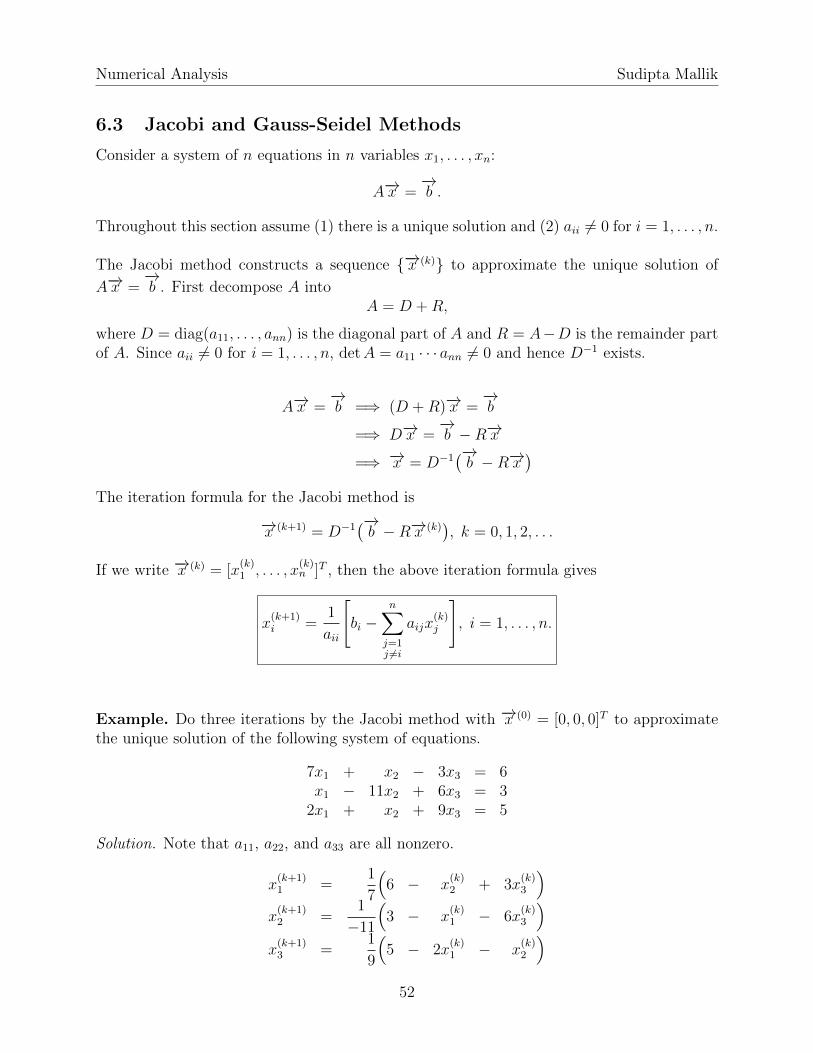
Numerical Analysis Sudipta Mallik
6.3 Jacobi and Gauss-Seidel Methods
Consider a system of n equations in n variables x1, . . . , xn:
A−→x =−→b .
Throughout this section assume (1) there is a unique solution and (2) aii 6= 0 for i = 1, . . . , n.
The Jacobi method constructs a sequence {−→x (k)} to approximate the unique solution of
A−→x =−→b . First decompose A into
A = D +R,
where D = diag(a11, . . . , ann) is the diagonal part of A and R = A−D is the remainder partof A. Since aii 6= 0 for i = 1, . . . , n, detA = a11 · · · ann 6= 0 and hence D−1 exists.
A−→x =−→b =⇒ (D +R)−→x =
−→b
=⇒ D−→x =−→b −R−→x
=⇒ −→x = D−1(−→b −R−→x
)The iteration formula for the Jacobi method is
−→x (k+1) = D−1(−→b −R−→x (k)
), k = 0, 1, 2, . . .
If we write −→x (k) = [x(k)1 , . . . , x
(k)n ]T , then the above iteration formula gives
x(k+1)i =
1
aii
[bi −
n∑j=1j 6=i
aijx(k)j
], i = 1, . . . , n.
Example. Do three iterations by the Jacobi method with −→x (0) = [0, 0, 0]T to approximatethe unique solution of the following system of equations.
7x1 + x2 − 3x3 = 6x1 − 11x2 + 6x3 = 3
2x1 + x2 + 9x3 = 5
Solution. Note that a11, a22, and a33 are all nonzero.
x(k+1)1 =
1
7
(6 − x
(k)2 + 3x
(k)3
)x(k+1)2 =
1
−11
(3 − x
(k)1 − 6x
(k)3
)x(k+1)3 =
1
9
(5 − 2x
(k)1 − x
(k)2
)52
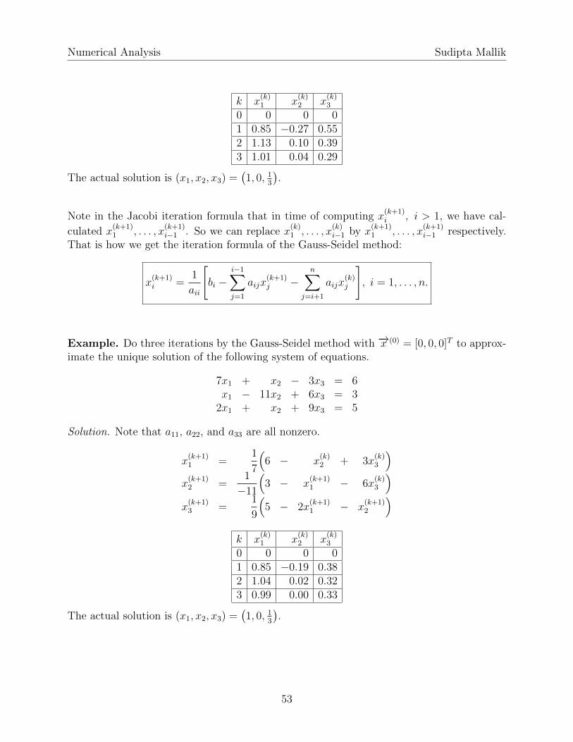
Numerical Analysis Sudipta Mallik
k x(k)1 x
(k)2 x
(k)3
0 0 0 01 0.85 −0.27 0.552 1.13 0.10 0.393 1.01 0.04 0.29
The actual solution is (x1, x2, x3) =(1, 0, 1
3
).
Note in the Jacobi iteration formula that in time of computing x(k+1)i , i > 1, we have cal-
culated x(k+1)1 , . . . , x
(k+1)i−1 . So we can replace x
(k)1 , . . . , x
(k)i−1 by x
(k+1)1 , . . . , x
(k+1)i−1 respectively.
That is how we get the iteration formula of the Gauss-Seidel method:
x(k+1)i =
1
aii
[bi −
i−1∑j=1
aijx(k+1)j −
n∑j=i+1
aijx(k)j
], i = 1, . . . , n.
Example. Do three iterations by the Gauss-Seidel method with −→x (0) = [0, 0, 0]T to approx-imate the unique solution of the following system of equations.
7x1 + x2 − 3x3 = 6x1 − 11x2 + 6x3 = 3
2x1 + x2 + 9x3 = 5
Solution. Note that a11, a22, and a33 are all nonzero.
x(k+1)1 =
1
7
(6 − x
(k)2 + 3x
(k)3
)x(k+1)2 =
1
−11
(3 − x
(k+1)1 − 6x
(k)3
)x(k+1)3 =
1
9
(5 − 2x
(k+1)1 − x
(k+1)2
)k x
(k)1 x
(k)2 x
(k)3
0 0 0 01 0.85 −0.19 0.382 1.04 0.02 0.323 0.99 0.00 0.33
The actual solution is (x1, x2, x3) =(1, 0, 1
3
).
53
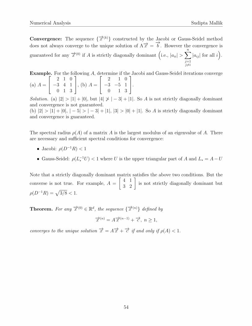
Numerical Analysis Sudipta Mallik
Convergence: The sequence {−→x (k)} constructed by the Jacobi or Gauss-Seidel method
does not always converge to the unique solution of A−→x =−→b . However the convergence is
guaranteed for any −→x (0) if A is strictly diagonally dominant(
i.e., |aii| >n∑j=1j 6=i
|aij| for all i)
.
Example. For the following A, determine if the Jacobi and Gauss-Seidel iterations converge
(a) A =
2 1 0−3 4 1
0 1 3
, (b) A =
2 1 0−3 −5 1
0 1 3
.
Solution. (a) |2| > |1| + |0|, but |4| ≯ | − 3| + |1|. So A is not strictly diagonally dominantand convergence is not guaranteed.(b) |2| > |1| + |0|, | − 5| > | − 3| + |1|, |3| > |0| + |1|. So A is strictly diagonally dominantand convergence is guaranteed.
The spectral radius ρ(A) of a matrix A is the largest modulus of an eigenvalue of A. Thereare necessary and sufficient spectral conditions for convergence:
• Jacobi: ρ(D−1R) < 1
• Gauss-Seidel: ρ(L−1∗ U) < 1 where U is the upper triangular part of A and L∗ = A−U
Note that a strictly diagonally dominant matrix satisfies the above two conditions. But the
converse is not true. For example, A =
[4 13 2
]is not strictly diagonally dominant but
ρ(D−1R) =√
3/8 < 1.
Theorem. For any −→x (0) ∈ Rd, the sequence {−→x (n)} defined by
−→x (n) = A−→x (n−1) +−→c , n ≥ 1,
converges to the unique solution −→x = A−→x +−→c if and only if ρ(A) < 1.
54
Numerical Analysis Sudipta Mallik
6.4 Eigenvalues: Power Method
Let A be an n×n matrix. If A−→x = λ−→x for some nonzero vector −→x and some scalar λ, thenλ is an eigenvalue of A and −→x is an eigenvector of A corresponding to λ.
Example. Consider A =
[1 20 3
], λ = 3, −→v =
[11
], −→u =
[−2
1
].
Since A−→v =
[1 20 3
] [11
]=
[33
]= 3
[11
]= λ−→v , 3 is an eigenvalue of A and −→v is an
eigenvector of A corresponding to the eigenvalue 3.
Since A−→u =
[1 20 3
] [−2
1
]=
[03
]6= λ
[−2
1
]= λ−→u for all scalars λ, −→u is not an
eigenvector of A.
The characteristic polynomial of A is det(A − λI) and its roots are the eigenvaluesof A. The eigenvectors of A corresponding to the eigenvalue λ are nonzero solutions of
(A− λI)−→x =−→O . The eigenspace of A corresponding to λ is
Nul(A− λI) = {−→x | (A− λI)−→x =−→O}.
The dominant eigenvalue of A is the eigenvalue of A with the largest modulus. Thespectral radius ρ(A) of A is the modulus of the dominant eigenvalue of A. For example, if3 and −4 are the eigenvalues of A, then −4 is the dominant eigenvalue of A and ρ(A) = 4.
In this section consider an n×n matrix A with real eigenvalues λ1 ≥ λ2 ≥ · · · ≥ λn. Assume
1. λ1 is the dominant eigenvalue of multiplicity 1 with eigenvector −→v1
2. There are n linearly independent eigenvectors −→v1 , . . . ,−→vn of A (i.e., A is diagonalizable)
The Power Method constructs a sequence {−→x (k)} defined by
−→x (k) =Ak−→x (0)
||Ak−→x (0)||, k ≥ 1
with an initial approximation −→x (0) to approximate an unit eigenvector corresponding to λ1:
Since −→v1 , . . . ,−→vn are n linearly independent eigenvectors, they span Rn and
−→x (0) = c1−→v1 + c2
−→v2 + · · ·+ cn−→vn,
for some scalars c1, c2, . . . , cn. We choose −→x (0) such that c1 6= 0. Then
55
Numerical Analysis Sudipta Mallik
−→x (0) = c1−→v1 + c2
−→v2 + · · ·+ cn−→vn
=⇒ A−→x (0) = c1A−→v1 + c2A
−→v2 + · · ·+ cnA−→vn
=⇒ A−→x (0) = c1λ1−→v1 + c2λ2
−→v2 + · · ·+ cnλn−→vn
=⇒ A2−→x (0) = c1λ1A−→v1 + c2λ2A
−→v2 + · · ·+ cnλnA−→vn
=⇒ A2−→x (0) = c1λ21−→v1 + c2λ
22−→v2 + · · ·+ cnλ
2n−→vn
· · ·=⇒ Ak−→x (0) = c1λ
k1−→v1 + c2λ
k2−→v2 + · · ·+ cnλ
kn−→vn
=⇒ Ak−→x (0) = λk1
(c1−→v1 + c2
(λ2λ1
)k−→v2 + · · ·+ cn
(λnλ1
)k−→vn
)
−→x (k) =Ak−→x (0)
||Ak−→x (0)||=
λk1
(c1−→v1 + c2
(λ2λ1
)k−→v2 + · · ·+ cn
(λnλ1
)k−→vn)∥∥∥∥λk1 (c1−→v1 + c2
(λ2λ1
)k−→v2 + · · ·+ cn
(λnλ1
)k−→vn)∥∥∥∥=
λk1
(c1−→v1 + c2
(λ2λ1
)k−→v2 + · · ·+ cn
(λnλ1
)k−→vn)|λk1|
∥∥∥∥(c1−→v1 + c2
(λ2λ1
)k−→v2 + · · ·+ cn
(λnλ1
)k−→vn)∥∥∥∥= ±
c1−→v1 + c2
(λ2λ1
)k−→v2 + · · ·+ cn
(λnλ1
)k−→vn∥∥∥∥c1−→v1 + c2
(λ2λ1
)k−→v2 + · · ·+ cn
(λnλ1
)k−→vn∥∥∥∥−→ ± c1
−→v1||c1−→v1 ||
= ± c1−→v1
|c1| · ||−→v1 ||= ±
−→v1||−→v1 ||
as k →∞.
Note that
A−→v1 = λ1−→v1 =⇒ −→v1TA−→v1 = λ1
−→v1T−→v1 =⇒ λ1 =−→v1TA−→v1−→v1T−→v1
If −→x (k) ≈ −→v1 , then
λ1 ≈ λ(k)1 :=
(−→x (k))TA−→x (k)
(−→x (k))T−→x (k).
Note
1. The power method does not work for −→x (0) = c1−→v1 + c2
−→v2 + · · ·+ cn−→vn when c1 = 0.
2. The rate convergence of {−→x (k)} is faster when
∣∣∣∣λ2λ1∣∣∣∣ is smaller, i.e., |λ2| << |λ1|.
56
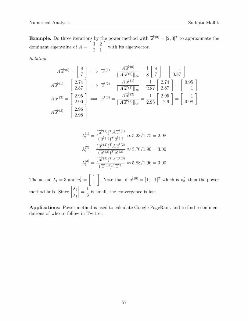
Numerical Analysis Sudipta Mallik
Example. Do three iterations by the power method with −→x (0) = [2, 3]T to approximate the
dominant eigenvalue of A =
[1 22 1
]with its eigenvector.
Solution.
A−→x (0) =
[87
]=⇒ −→x (1) =
A−→x (0)
||A−→x (0)||∞=
1
8
[87
]=
[1
0.87
]A−→x (1) =
[2.742.87
]=⇒ −→x (2) =
A−→x (1)
||A−→x (1)||∞=
1
2.87
[2.742.87
]=
[0.95
1
]A−→x (2) =
[2.952.90
]=⇒ −→x (3) =
A−→x (2)
||A−→x (2)||∞=
1
2.95
[2.952.9
]=
[1
0.98
]A−→x (3) =
[2.962.98
]
λ(1)1 =
(−→x (1))TA−→x (1)
(−→x (1))T−→x (1)≈ 5.23/1.75 = 2.98
λ(2)1 =
(−→x (2))TA−→x (2)
(−→x (2))T−→x (2)≈ 5.70/1.90 = 3.00
λ(3)1 =
(−→x (3))TA−→x (3)
(−→x (3))T−→x 3)≈ 5.88/1.96 = 3.00
The actual λ1 = 3 and −→v1 =
[11
]. Note that if −→x (0) = [1,−1]T which is −→v2 , then the power
method fails. Since
∣∣∣∣λ2λ1∣∣∣∣ =
1
3is small, the convergence is fast.
Applications: Power method is used to calculate Google PageRank and to find recommen-dations of who to follow in Twitter.
57
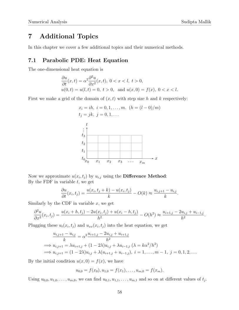
Numerical Analysis Sudipta Mallik
7 Additional Topics
In this chapter we cover a few additional topics and their numerical methods.
7.1 Parabolic PDE: Heat Equation
The one-dimensional heat equation is
∂u
∂t(x, t) = α2∂
2u
∂x2(x, t), 0 < x < l, t > 0,
u(0, t) = u(l, t) = 0, t > 0, and u(x, 0) = f(x), 0 < x < l.
First we make a grid of the domain of (x, t) with step size h and k respectively:
xi = ih, i = 0, 1, . . . ,m. (h = (l − 0)/m)
tj = jk, j = 0, 1, . . .
x0 x1 x2 x3t0
t1
t2
t3
...
x
t
· · · xm
Now we approximate u(xi, tj) by ui,j using the Difference Method:By the FDF in variable t, we get
∂u
∂t(xi, tj) =
u(xi, tj + k)− u(xi, tj)
k−O(k) ≈ ui,j+1 − ui,j
k.
Similarly by the CDF in variable x, we get
∂2u
∂x2(xi, tj) =
u(xi + h, tj)− 2u(xi, tj) + u(xi − h, tj)h2
−O(h2) ≈ ui+1,j − 2ui,j + ui−1,jh2
.
Plugging these ut(xi, tj) and uxx(xi, tj) into the heat equation, we get
ui,j+1 − ui,jk
= α2ui+1,j − 2ui,j + ui+1,j
h2
=⇒ ui,j+1 = λui+1,j + (1− 2λ)ui,j + λui−1,j (λ = kα2/h2)
=⇒ ui,j+1 = (1− 2λ)ui,j + λ(ui+1,j + ui−1,j), i = 1, . . . ,m− 1, j = 0, 1, 2, . . .
By the initial condition u(x, 0) = f(x), we have
u0,0 = f(x0), u1,0 = f(x1), . . . , um,0 = f(xm).
Using u0,0, u1,0, . . . , um,0, we can find u0,1, u1,1, . . . , um,1 and so on at different values of tj.
58
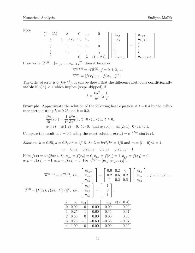
Numerical Analysis Sudipta Mallik
Note (1− 2λ) λ 0 . . . 0
λ (1− 2λ). . . . . .
...
0. . . . . . . . . 0
.... . . . . . . . . λ
0 . . . 0 λ (1− 2λ)
u1,ju2,j......um−1,j
=
u1,j+1
u2,j+1......um−1,j+1
If we write −→u (j) = [u1,j, . . . , um−1,j]
T , then it becomes
−→u (j+1) = A−→u (j), j = 0, 1, 2, . . .−→u (0) = [f(x1), . . . , f(xm−1)]
T .
The order of error is O(k+h2). It can be shown that the difference method is conditionallystable if ρ(A) < 1 which implies (steps skipped) if
λ =kα2
h2≤ 1
2.
Example. Approximate the solution of the following heat equation at t = 0.4 by the differ-ence method using h = 0.25 and k = 0.2.
∂u
∂t(x, t) =
1
16
∂2u
∂x2(x, t), 0 < x < 1, t ≥ 0,
u(0, t) = u(1, t) = 0, t > 0, and u(x, 0) = sin(2πx), 0 < x < 1.
Compare the result at t = 0.4 using the exact solution u(x, t) = e−π2t/4 sin(2πx).
Solution. h = 0.25, k = 0.2, α2 = 1/16. So λ = kα2/h2 = 1/5 and m = (l − 0)/h = 4.
x0 = 0, x1 = 0.25, x2 = 0.5, x3 = 0.75, x4 = 1
Here f(x) = sin(2πx). So u0,0 = f(x0) = 0, u1,0 = f(x1) = 1, u2,0 = f(x2) = 0,u3,0 = f(x3) = −1, u4,0 = f(x4) = 0. For −→u (j) = [u1,j, u2,j, u3,j]
T ,
−→u (j+1) = A−→u (j), i.e.,
u1,j+1
u2,j+1
u3,j+1
=
0.6 0.2 00.2 0.6 0.20 0.2 0.6
u1,ju2,ju3,j
, j = 0, 1, 2, . . .
−→u (0) = [f(x1), f(x2), f(x3)]T , i.e.,
u1,0u2,0u3,0
=
10−1
.i xi ui,0 ui,1 ui,2 u(xi, 0.4)0 0.00 0 0.00 0.00 0.001 0.25 1 0.60 0.36 0.372 0.50 0 0.00 0.00 0.003 0.75 −1 −0.60 −0.36 −0.374 1.00 0 0.00 0.00 0.00
59
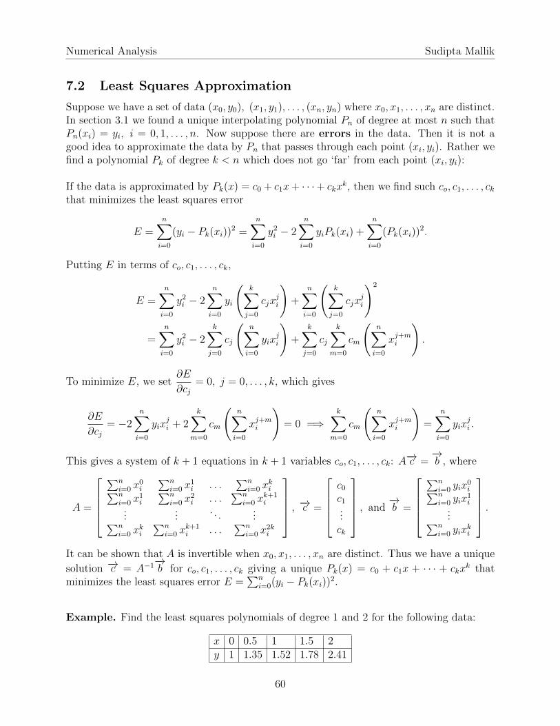
Numerical Analysis Sudipta Mallik
7.2 Least Squares Approximation
Suppose we have a set of data (x0, y0), (x1, y1), . . . , (xn, yn) where x0, x1, . . . , xn are distinct.In section 3.1 we found a unique interpolating polynomial Pn of degree at most n such thatPn(xi) = yi, i = 0, 1, . . . , n. Now suppose there are errors in the data. Then it is not agood idea to approximate the data by Pn that passes through each point (xi, yi). Rather wefind a polynomial Pk of degree k < n which does not go ‘far’ from each point (xi, yi):
If the data is approximated by Pk(x) = c0 + c1x+ · · ·+ ckxk, then we find such co, c1, . . . , ck
that minimizes the least squares error
E =n∑i=0
(yi − Pk(xi))2 =n∑i=0
y2i − 2n∑i=0
yiPk(xi) +n∑i=0
(Pk(xi))2.
Putting E in terms of co, c1, . . . , ck,
E =n∑i=0
y2i − 2n∑i=0
yi
(k∑j=0
cjxji
)+
n∑i=0
(k∑j=0
cjxji
)2
=n∑i=0
y2i − 2k∑j=0
cj
(n∑i=0
yixji
)+
k∑j=0
cj
k∑m=0
cm
(n∑i=0
xj+mi
).
To minimize E, we set∂E
∂cj= 0, j = 0, . . . , k, which gives
∂E
∂cj= −2
n∑i=0
yixji + 2
k∑m=0
cm
(n∑i=0
xj+mi
)= 0 =⇒
k∑m=0
cm
(n∑i=0
xj+mi
)=
n∑i=0
yixji .
This gives a system of k + 1 equations in k + 1 variables co, c1, . . . , ck: A−→c =
−→b , where
A =
∑n
i=0 x0i
∑ni=0 x
1i . . .
∑ni=0 x
ki∑n
i=0 x1i
∑ni=0 x
2i . . .
∑ni=0 x
k+1i
......
. . ....∑n
i=0 xki
∑ni=0 x
k+1i . . .
∑ni=0 x
2ki
, −→c =
c0c1...ck
, and−→b =
∑n
i=0 yix0i∑n
i=0 yix1i
...∑ni=0 yix
ki
.It can be shown that A is invertible when x0, x1, . . . , xn are distinct. Thus we have a unique
solution −→c = A−1−→b for co, c1, . . . , ck giving a unique Pk(x) = c0 + c1x + · · · + ckx
k thatminimizes the least squares error E =
∑ni=0(yi − Pk(xi))2.
Example. Find the least squares polynomials of degree 1 and 2 for the following data:
x 0 0.5 1 1.5 2y 1 1.35 1.52 1.78 2.41
60
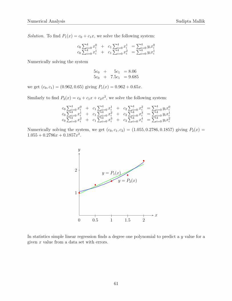
Numerical Analysis Sudipta Mallik
Solution. To find P1(x) = c0 + c1x, we solve the following system:
c0∑4
i=0 x0i + c1
∑4i=0 x
1i =
∑4i=0 yix
0i
c0∑4
i=0 x1i + c1
∑4i=0 x
2i =
∑4i=0 yix
1i
Numerically solving the system
5c0 + 5c1 = 8.065c0 + 7.5c1 = 9.685
we get (c0, c1) = (0.962, 0.65) giving P1(x) = 0.962 + 0.65x.
Similarly to find P2(x) = c0 + c1x+ c2x2, we solve the following system:
c0∑4
i=0 x0i + c1
∑4i=0 x
1i + c2
∑4i=0 x
2i =
∑4i=0 yix
0i
c0∑4
i=0 x1i + c1
∑4i=0 x
2i + c2
∑4i=0 x
3i =
∑4i=0 yix
1i
c0∑4
i=0 x2i + c1
∑4i=0 x
3i + c2
∑4i=0 x
4i =
∑4i=0 yix
2i
Numerically solving the system, we get (c0, c1, c2) = (1.055, 0.2786, 0.1857) giving P2(x) =1.055 + 0.2786x+ 0.1857x2.
x
y
0.5 1 1.5 2
1
2
0
y = P1(x)
y = P2(x)
In statistics simple linear regression finds a degree one polynomial to predict a y value for agiven x value from a data set with errors.
61
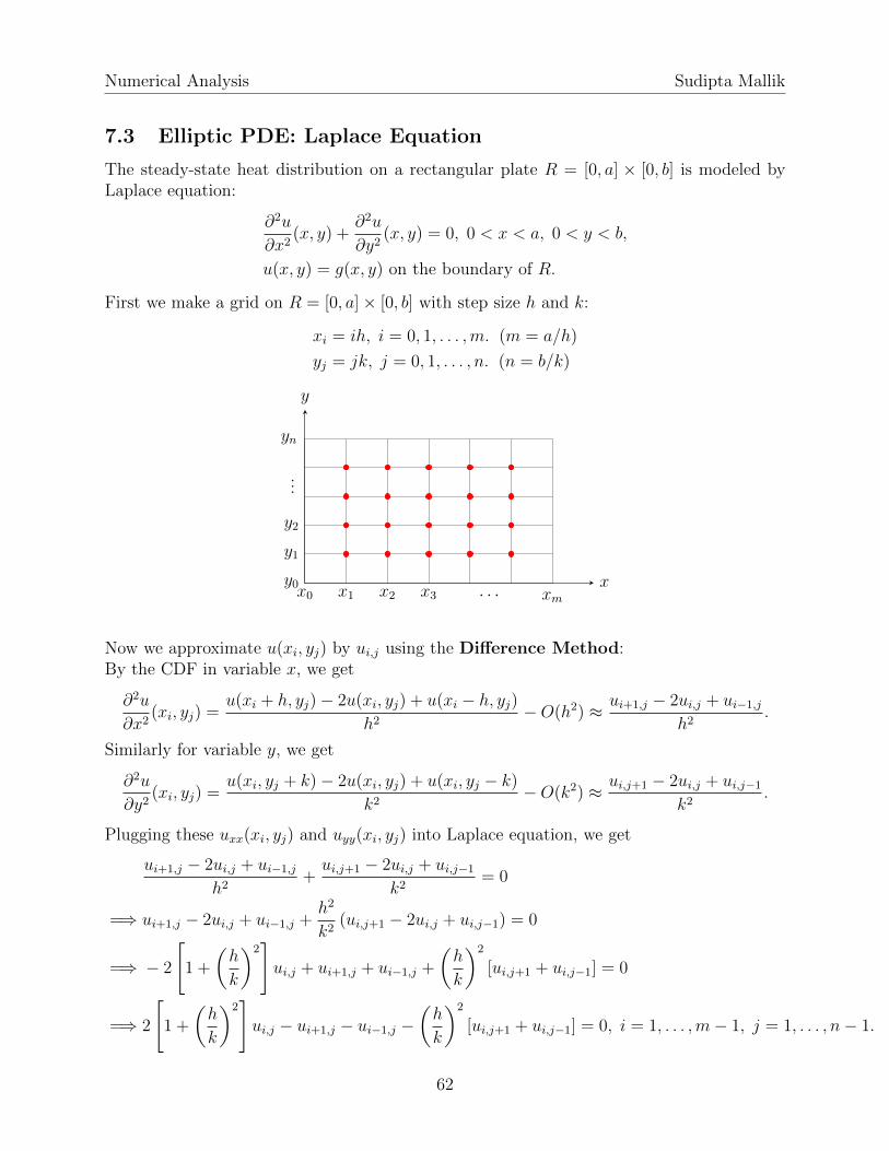
Numerical Analysis Sudipta Mallik
7.3 Elliptic PDE: Laplace Equation
The steady-state heat distribution on a rectangular plate R = [0, a] × [0, b] is modeled byLaplace equation:
∂2u
∂x2(x, y) +
∂2u
∂y2(x, y) = 0, 0 < x < a, 0 < y < b,
u(x, y) = g(x, y) on the boundary of R.
First we make a grid on R = [0, a]× [0, b] with step size h and k:
xi = ih, i = 0, 1, . . . ,m. (m = a/h)
yj = jk, j = 0, 1, . . . , n. (n = b/k)
x0 x1 x2 x3y0
y1
y2
x
y
· · ·
...
xm
yn
Now we approximate u(xi, yj) by ui,j using the Difference Method:By the CDF in variable x, we get
∂2u
∂x2(xi, yj) =
u(xi + h, yj)− 2u(xi, yj) + u(xi − h, yj)h2
−O(h2) ≈ ui+1,j − 2ui,j + ui−1,jh2
.
Similarly for variable y, we get
∂2u
∂y2(xi, yj) =
u(xi, yj + k)− 2u(xi, yj) + u(xi, yj − k)
k2−O(k2) ≈ ui,j+1 − 2ui,j + ui,j−1
k2.
Plugging these uxx(xi, yj) and uyy(xi, yj) into Laplace equation, we get
ui+1,j − 2ui,j + ui−1,jh2
+ui,j+1 − 2ui,j + ui,j−1
k2= 0
=⇒ ui+1,j − 2ui,j + ui−1,j +h2
k2(ui,j+1 − 2ui,j + ui,j−1) = 0
=⇒ − 2
[1 +
(h
k
)2]ui,j + ui+1,j + ui−1,j +
(h
k
)2
[ui,j+1 + ui,j−1] = 0
=⇒ 2
[1 +
(h
k
)2]ui,j − ui+1,j − ui−1,j −
(h
k
)2
[ui,j+1 + ui,j−1] = 0, i = 1, . . . ,m− 1, j = 1, . . . , n− 1.
62
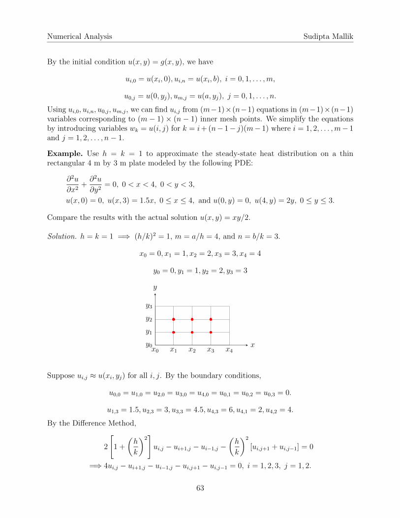
Numerical Analysis Sudipta Mallik
By the initial condition u(x, y) = g(x, y), we have
ui,0 = u(xi, 0), ui,n = u(xi, b), i = 0, 1, . . . ,m,
u0,j = u(0, yj), um,j = u(a, yj), j = 0, 1, . . . , n.
Using ui,0, ui,n, u0,j, um,j, we can find ui,j from (m−1)×(n−1) equations in (m−1)×(n−1)variables corresponding to (m− 1)× (n− 1) inner mesh points. We simplify the equationsby introducing variables wk = u(i, j) for k = i+ (n− 1− j)(m− 1) where i = 1, 2, . . . ,m− 1and j = 1, 2, . . . , n− 1.
Example. Use h = k = 1 to approximate the steady-state heat distribution on a thinrectangular 4 m by 3 m plate modeled by the following PDE:
∂2u
∂x2+∂2u
∂y2= 0, 0 < x < 4, 0 < y < 3,
u(x, 0) = 0, u(x, 3) = 1.5x, 0 ≤ x ≤ 4, and u(0, y) = 0, u(4, y) = 2y, 0 ≤ y ≤ 3.
Compare the results with the actual solution u(x, y) = xy/2.
Solution. h = k = 1 =⇒ (h/k)2 = 1, m = a/h = 4, and n = b/k = 3.
x0 = 0, x1 = 1, x2 = 2, x3 = 3, x4 = 4
y0 = 0, y1 = 1, y2 = 2, y3 = 3
x0 x1 x2 x3 x4y0
y1
y2
y3
x
y
Suppose ui,j ≈ u(xi, yj) for all i, j. By the boundary conditions,
u0,0 = u1,0 = u2,0 = u3,0 = u4,0 = u0,1 = u0,2 = u0,3 = 0.
u1,3 = 1.5, u2,3 = 3, u3,3 = 4.5, u4,3 = 6, u4,1 = 2, u4,2 = 4.
By the Difference Method,
2
[1 +
(h
k
)2]ui,j − ui+1,j − ui−1,j −
(h
k
)2
[ui,j+1 + ui,j−1] = 0
=⇒ 4ui,j − ui+1,j − ui−1,j − ui,j+1 − ui,j−1 = 0, i = 1, 2, 3, j = 1, 2.
63
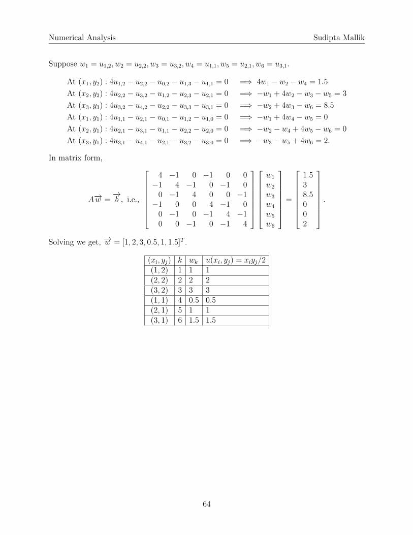
Numerical Analysis Sudipta Mallik
Suppose w1 = u1,2, w2 = u2,2, w3 = u3,2, w4 = u1,1, w5 = u2,1, w6 = u3,1.
At (x1, y2) : 4u1,2 − u2,2 − u0,2 − u1,3 − u1,1 = 0 =⇒ 4w1 − w2 − w4 = 1.5
At (x2, y2) : 4u2,2 − u3,2 − u1,2 − u2,3 − u2,1 = 0 =⇒ −w1 + 4w2 − w3 − w5 = 3
At (x3, y3) : 4u3,2 − u4,2 − u2,2 − u3,3 − u3,1 = 0 =⇒ −w2 + 4w3 − w6 = 8.5
At (x1, y1) : 4u1,1 − u2,1 − u0,1 − u1,2 − u1,0 = 0 =⇒ −w1 + 4w4 − w5 = 0
At (x2, y1) : 4u2,1 − u3,1 − u1,1 − u2,2 − u2,0 = 0 =⇒ −w2 − w4 + 4w5 − w6 = 0
At (x3, y1) : 4u3,1 − u4,1 − u2,1 − u3,2 − u3,0 = 0 =⇒ −w3 − w5 + 4w6 = 2.
In matrix form,
A−→w =−→b , i.e.,
4 −1 0 −1 0 0−1 4 −1 0 −1 0
0 −1 4 0 0 −1−1 0 0 4 −1 0
0 −1 0 −1 4 −10 0 −1 0 −1 4
w1
w2
w3
w4
w5
w6
=
1.538.5002
.
Solving we get, −→w = [1, 2, 3, 0.5, 1, 1.5]T .
(xi, yj) k wk u(xi, yj) = xiyj/2(1, 2) 1 1 1(2, 2) 2 2 2(3, 2) 3 3 3(1, 1) 4 0.5 0.5(2, 1) 5 1 1(3, 1) 6 1.5 1.5
64


![Numerical Integration and Differentiation Quantitative ... · Numerical Integration and Di erentiation Quantitative Macroeconomics [Econ 5725] Raul Santaeul alia-Llopis Washington](https://img.pdfslide.us/doc/110x75/5b68494a7f8b9a6f778c9014/numerical-integration-and-differentiation-quantitative-numerical-integration.jpg)