Dynamic Pricing and Product Di erentiation with Cost

Dynamic Pricing and Product Differentiationwith Cost Uncertainty and Learning

N. Bora Keskin, John R. Birge

Submitted to M&SOM Service SIG 2015 Conference

Dynamic Pricing and Product Differentiation

with Cost Uncertainty and Learning(Authors’ names blinded for peer review)

Motivated by applications in the health insurance industry, we consider a seller who designs and sells a set of ver-

tically differentiated products to a population of quality-sensitive customers. The seller’s business environment

entails an uncertainty about production costs. We characterize the seller’s optimal price-quality schedule in the

cases of: (a) static cost uncertainty, and (b) dynamic learning about cost uncertainty through noisy observations

on an underlying cost curve. We prove that the seller’s optimal quality allocations in (a) and (b) stand in stark

contrast: While a seller facing static cost uncertainty degrades the quality in its product offering, a dynami-

cally learning seller improves the quality of its products to accelerate information accumulation. In the case of

dynamic learning, we prove that the seller exercises the most extreme experimentation on less quality-sensitive

customers. We also extend our results to the cases of commonly used regulations in health insurance industry,

and show how such regulations moderate the interplay between uncertainty and learning.

Key words : Dynamic programming, Bayesian learning, pricing, self-selection, exploration-exploitation.

1. Introduction

Pricing and product differentiation decisions have dual goals: First, they can help firms design prod-

ucts for the varying needs of potential customers, and increase profits by implementing a menu of

products from which customers with some unobservable characteristics can self-select. Secondly, these

decisions can also serve as tools to learn about the potential uncertainties present in a firm’s business

environment, thereby enabling the firm to adaptively improve its product design and increase future

profits. Some of the key questions in this context are the following: If a firm’s business environment

entails uncertainties that can influence production costs, how do these uncertainties affect the firm’s

optimal pricing and product differentiation decisions? What are the benefits and consequences of using

these decisions as learning tools? How should a firm design its product offering to learn optimally?

This paper sheds light on the aforementioned questions by introducing a dynamic pricing and

production differentiation problem with cost uncertainty and learning. In our problem formulation,

we consider a firm that faces an uncertainty about its production costs. There is a cost curve that

gives the cost of production as a function of a certain quality that makes the product more desirable

to customers. We model the firm’s uncertainty about costs as a Bernoulli belief distribution on two

possible cost curves; that is, the firm’s production costs may turn out to be high or low due to

the unresolved uncertainty in the firm’s business environment. To measure the effect of this cost

uncertainty, we use as a benchmark the case of perfect cost information, which corresponds to the

1

Authors’ names blinded for peer review

2 Article submitted to M&SOM Service SIG 2015 Conference

expected profit performance of a clairvoyant who knows the underlying cost curve. In this setting, we

characterize the firm’s optimal pricing and production differentiation policy and show that the presence

of cost uncertainty leads to a quality degradation in the firm’s optimal policy, relative to the expected

quality allocation of the clairvoyant. In stark contrast, if the firm can make sequential observations on

the cost curve, and dynamically update its product offering, we show that the firm optimally improves

the qualities in its product offering to accelerate learning. Assuming that the population of customers

are heterogenous in terms of their sensitivity to quality, we examine the structure of the firm’s optimal

learning policy and identify that the firm exercises more experimentation on less quality-sensitive

customers. Furthermore, we generalize our analysis to the cases of commonly used regulations that

subsidize quality in practice, namely a free outside option with positive but low quality and price

subsidies.

Vertically differentiated products are present in many industries. A notable example is the health

insurance industry where insurance contracts are designed and priced to satisfy significantly vary-

ing healthcare needs of insurance customers. Thus, insurance companies can sell a range of products

tailored to their customers’ differing preferences. However, when there is a new regulation or a tech-

nological innovation, an insurance company’s cost of providing the same service can shift upward or

downward, creating a cost uncertainty from the company’s perspective. In a recent study, Kowalski

(2014) reports that the introduction of the Affordable Care Act (ACA) in the United States has led

to increased average costs of health insurance companies in some states, but reduced average costs in

some others. According to Kowalski (2014), some of this effect can be explained by technological issues

such as the glitches in the enrollment system and political issues such as the degree of cooperation

between the federal and state governments. Moreover, the introduction of such regulations enlarges

the insurance companies’ customer base to include individuals with little or no understanding of how

to use health insurance (Goodnough 2014), creating further uncertainty about the potential cost of

providing service. Motivated by this application, our paper focuses on the possible theoretical impli-

cations of cost uncertainties on a firm’s pricing and product design decisions. To that end, we develop

a stylized framework of dynamic pricing and product differentiation with cost uncertainty, with the

hope of gaining insights into more realistic product design problems.

Summary of main contributions. This paper makes four contributions to the literature on

learning and earning. First, we develop and analyze a dynamic learning model that extends the

research literature on model uncertainty and dynamic learning to the case of self-selection mechanisms.

As will be discussed below, the vast majority of the related research has focused on either the dynamic

control of posted prices or the optimal timing of new technology adoption. Our paper shows how


Article submitted to M&SOM Service SIG 2015 Conference 3

product design decisions such as product differentiation and pricing can be jointly used a learning

tool, and we hope that this work will lead to further research on dynamic product design with cost

uncertainty. Our analysis of the dynamic learning model provides key tools for further studying

dynamic nonlinear pricing problems with model uncertainty and learning. In our analysis, we define a

conditional value function that is adapted to the quality choices of customers and then characterize the

optimal pricing and quality allocation decisions based on the conditional value of learning. Second, our

characterization of the optimal product offering identifies two starkly contrasting effects in the cases

of: (a) static cost uncertainty, and (b) dynamic learning about cost uncertainty. While the presence of

cost uncertainty makes a firm degrade the quality in its product offering, an opportunity to learn about

this cost uncertainty makes the firm improve the quality of its products. It is perhaps worth noting that

our quality degradation result, which is driven by uncertainty, is distinct from the standard quality

degradation results in nonlinear pricing theory, which are usually caused by monopolistic distortion.

Third, we provide key structural insights into the design of optimal experimentation for dynamic

learning about cost uncertainty. Our analysis reveals that a firm projects the value of learning onto its

product offering by improving the quality uniformly for all products and implementing the strongest

quality improvement for the products that target less quality-sensitive customers. We believe that this

structure of our optimal policy can provide a practical guideline for designing products in presence

of cost uncertainty. Finally, we extend our analysis to the case of commonly used regulations in the

health insurance industry, shedding some light on how these regulations would moderate the interplay

between static uncertainty and dynamic learning, and how a firm should design its product offering

under such regulations.

Related literature. Our work is related to three streams of research, namely (i) the economics

literature on nonlinear pricing and self-selection, (ii) the decision analysis literature on dynamic pro-

gramming with Bayesian learning, and (iii) the operations research and management science (OR/MS)

and economics literature on dynamic pricing with model uncertainty and learning.

With regard to (i), there is a rich economics literature on vertical product differentiation and self-

selection. The origins of this literature can be traced back to Mussa and Rosen (1978) and Maskin

and Riley (1984), who have formulated and analyzed the problem of designing and pricing a set of

products to maximize profits earned from a population of quality-sensitive customers. A key result

derived in this framework is that monopolistic pricing reduces the quality in a seller’s product offering,

relative to perfectly competitive pricing. Besanko, Donnenfeld and White (1987, 1988) have studied

how this quality distortion due to monopoly power can be remedied by implementing regulations

such as a price ceiling or minimum quality standards, which are motivated by the regulations in the



cable television industry in the United States. Another paper that studies the monopoly distortion

with regulations is due to Jullien (2000), who has investigated sufficient conditions for customers’

participation in the presence of price cap regulations. Rochet and Stole (2002) have extended this

literature by introducing randomness to the customers’ valuations for outside options, showing that

such random outside options can eliminate some of the monopoly distortion effect. More recently,

Bergemann, Shen, Xu and Yeh (2012) have studied a nonlinear pricing problem with a finite menu

constraint, characterizing the loss due to the limitation to a finite menu of products. To the best of our

knowledge, the aforementioned economics literature on nonlinear pricing and product differentiation

has not focused on cost model uncertainty and dynamic learning. Our work contributes to this litera-

ture by introducing and analyzing the optimal dynamic control of a nonlinear price-quality schedule

in the presence of cost model uncertainty and learning. In particular, we show that the presence of a

static cost uncertainty could result in further quality reduction in a monopolist’s product offering and

that a dynamically learning monopolist can improve quality significantly to increase future gains.

With regard to (ii), a main focus of attention has been the analysis of technology adoption problems

with uncertainty about benefits and costs of adoption. In this context, McCardle (1985) and Lippman

and McCardle (1987) have studied optimal stopping problems in which a firm explores the profitability

of a technology to decide whether to adopt the technology or not and have characterized the optimal

technology adoption policies in their settings. Ulu and Smith (2009) have analyzed a more general

model of technology adoption involving non-stationary technologies and fairly general signal processes

and have derived key comparative statics results regarding the optimal policy. In a more recent study,

Smith and Ulu (2012) have considered the case of repeated technology adoption decisions with time-

varying costs and benefits, showing that the structure of the optimal policy for repeated technology

adoptions differs significantly from the one for single technology adoption. Apart from these studies,

Mazzola and McCardle (1996) have focused on a production planning problem where a firm has

recently adopted a new technology and faces an uncertainty about its learning curve and have showed

that in the presence of learning-curve uncertainty the firm’s optimal production does not necessarily

increase with cumulative production. Like the majority of the above studies, our paper employs a

Bayesian decision model based on dynamic programming. But, the problem we study is a dynamic

control problem rather than an optimal stopping problem, which is used in many of the studies

mentioned above (see, e.g., McCardle 1985, Lippman and McCardle 1987, Ulu and Smith 2009). More

importantly, the decisions in our framework, namely nonlinear price-quality schedules of the firm,

are continuous mappings and hence have very high dimensions compared to the decision variables in

the aforementioned decision analysis studies. To analyze this framework, we introduce and study a



conditional value function that is adapted to the latest customer choice observed by the firm, and

provide an analysis of how to use high dimensional price-quality schedules as a dynamic learning tool.

With regard to (iii), there has been substantial effort to study the tradeoff between learning and

earning in dynamic pricing applications. In the economics literature, Keller and Rady (1999) have

studied a continuous-time stochastic control problem in which a firm is uncertain about the time-

varying demand curve for its product and learns about the unknown demand curve by experimenting

with sales quantities, and have characterized the optimal policy in their setting. Following this work,

Bergemann and Valimaki (2000) and Keller and Rady (2003) have formulated and analyzed duopolis-

tic competition models for dynamic pricing. Bergemann and Valimaki (2000) have considered a market

with an incumbent seller and an entrant, assuming that buyers and sellers are uncertain about the

value of the entrant’s product and receive publicly observable signals about the unknown product

value. In this setting, they have analyzed the Markov perfect equilibrium that describes the pric-

ing strategies of the sellers. On the other hand, Keller and Rady (2003) have considered two sellers

who are uncertain about the parameters of the demand curves for their substitutable products, and

have characterized the sellers’ pricing strategies in a Markov perfect equilibrium. There are several

distinguishing features that differentiate our work from these studies. First, as explained in the pre-

ceding paragraph, our model involves the dynamic control of a price-quality schedule. To be more

precise, the seller in our problem dynamically designs a continuum of price-quality pairs throughout

the selling horizon, which separates our work from standard dynamic pricing problems in terms of

modeling and analysis. Second, unlike the above studies, we investigate the impact of cost uncertainty

on the optimal policy, and identify the contrasting effects of static cost uncertainty and dynamic learn-

ing about cost uncertainty. This analysis provides unique insights about how to design experiments

with a price-quality schedule with the aim of resolving an underlying cost uncertainty. Third, we

use discrete-time dynamic programming rather than continuous-time stochastic control, which makes

our mathematical tools and proof techniques distinct. On top of the related economics literature dis-

cussed above, there has been recent interest in the OR/MS literature on dynamic pricing problems

with demand learning. An early study in this research stream is due to Aviv and Pazgal (2005),

who analyze a dynamic pricing problem in which a firm sells a single product while facing Bayesian

uncertainty about the demand curve for its product. More recently, Araman and Caldentey (2009),

Farias and van Roy (2010), and Harrison, Keskin and Zeevi (2012) have further investigated dynamic

pricing with Bayesian demand learning and characterized well-performing policies that balance the

tradeoff between learning and earning. A common feature of these studies is that they focus on the

pricing of a single product, rather than multiple products. While the extension from single-product



pricing to multi-product pricing has been recently studied by Keskin and Zeevi (2014) and den Boer

(2014), these papers, too, consider a pre-determined set of products. In summary, the aforementioned

OR/MS research on dynamic pricing and learning has essentially focused on using dynamic posted-

price mechanisms as experimentation tools, either for a single product or for an exogenously given set

of products. Unlike this research stream, we study the possibility of jointly using pricing and product

differentiation decisions as learning tools and explore how learning affects the design of self-selection

mechanisms. Moreover, the vast majority of the recent OR/MS work on dynamic pricing and learning

have concentrated on near-optimal learning policies, whereas we investigate in this paper the structure

of exactly optimal learning policies for dynamic pricing and product differentiation.

Organization of the paper. This paper is organized as follows. Section 2 describes the basic

problem formulation and analyzes the case of static cost uncertainty. In Section 3, we extend our

basic problem formulation and analysis to the case of dynamic learning. Section 4 investigates how

regulations moderate the effects of static cost uncertainty and dynamic learning. Finally, Section 5

concludes with possible extensions of this study. Proofs of key results are deferred to appendices.

2. Problem Formulation and Analysis of Static Cost Uncertainty

Consider a firm that sells a product that can be produced at different levels of quality. The product’s

quality q takes values in Q = [0,∞). The firm can produce a range of differentiated qualities in Qand can charge a different price for every distinct quality level in its product offering. If a customer

purchases a product with quality q at price p, then the customer derives a net utility of

U(θ, q, p) = θq− p , (2.1)

where θ denotes the customer’s sensitivity to quality. There is a population of potential customers

whose quality sensitivities are unobservable and distributed according to a density function f(θ) on

Θ = [θmin, θmax]. We assume that f(θ) has increasing failure rate; i.e., f(θ)/F(θ) increases in θ, where

F (θ) =∫ θmax

θf(ξ)dξ. (An important example that satisfies this property is the uniform distribution;

other noteworthy examples are Gaussian and exponential distributions.) The expected cost of produc-

ing and selling one unit of the product at quality level q is c(q). Due to technological innovations and

operational regulations that can potentially happen after the time of sales, the firm is uncertain about

the cost curve c(·) at the time of sales. We model this uncertainty via a Bernoulli prior distribution

on two possible cost curves. Prior to sales, nature chooses either c0(·) or c1(·) as the underlying cost

curve, where ci(q) = aiq2 for i = 0,1, and 0 < a0 < a1 < ∞. Without observing the underlying cost

curve, the firm initially believes that

c(·) =

{c1(·) with probability b

c0(·) with probability 1 − b,(2.2)



where b∈ [0,1]. We hereafter refer to b as the firm’s prior belief. To serve its customers, the firm offers

the product with quality q at a price P (q) for all q ∈ Q. As will be explained below, the firm can

implement a selling mechanism S = {(p(θ), q(θ)) : θ ∈ Θ} that assigns a price-quality pair (p(θ), q(θ))

to each quality sensitivity parameter θ, ensuring that every customer selects the price-quality pair

assigned to its quality sensitivity. For brevity, we hereafter refer to a pair of pricing and quality

allocation functions, p : Θ → R+ and q : Θ → Q respectively, as a product offering. Therefore, the firm’s

objective is to choose a product offering to maximize the expected profit from all potential customers;

that is, the firm solves the following problem:

V (b) = maxp(·),q(·)

{∫ θmax

θmin

(p(θ) −C

(b, q(θ)

))f(θ)dθ

}(2.3a)

s.t. θq(θ) − p(θ) ≥ θq(θ) − p(θ) for all θ, θ ∈ Θ, (2.3b)

θq(θ) − p(θ) ≥ 0 for all θ ∈ Θ, (2.3c)

q(θ) ≥ 0 for all θ ∈ Θ, (2.3d)

where C(b, q) = bc1(q)+(1− b)c0(q) is the expected cost of production when the firm’s prior belief is b

and the quality level is q. The constraints (2.3b) are usually referred to as incentive compatibility (IC)

constraints, which ensure that a customer with quality sensitivity parameter θ prefers (p(θ), q(θ)) to

any other price-quality pair in the firm’s product offering. The constraints (2.3c) are referred to as

individual rationality (IR) constraints, which ensure that a customer with quality sensitivity parameter

θ prefers (p(θ), q(θ)) to an outside option that offers a net utility of zero. The optimal objective value

of the problem in (2.3), which is denoted by V (b), is the expected maximized profit as a function of

the firm’s initial belief b.

Our first goal is to express the optimization problem in (2.3) in a simpler form. To that end,

we start with characterizing a set of conditions that describe the constraints of this problem. By

standard results in nonlinear pricing theory (see, e.g., Mussa and Rosen 1978), we have the following

proposition.

Proposition 1. (incentive compatibility and individual rationality)

(i) The IC constraints (2.3b) hold if and only if q(·) is increasing and differentiable almost every-

where, and p′(θ) = θq′(θ) for θ ∈ Θ, except on a set of measure zero.

(ii) Assume that the IC constraints (2.3b) hold, and that θmin q(θmin) − p(θmin) = 0. Then the IR

constraints (2.3c) also hold.

Proposition 1(i) transforms the constraints of (2.3) into a local differential relationship between

pricing and quality allocation functions. In particular, it prescribes a particular marginal price increase



for an additional unit of quality. Using Proposition 1, we deduce that the pricing function p(·) must

satisfy the following to induce the IC and IR constraints:

p(θ) = p(θmin) +

∫ θ

θmin

p′(ξ)dξ(a)= p(θmin) +

∫ θ

θmin

ξq′(ξ)dξ

(b)= p(θmin) + θq(θ) − θmin q(θmin) −

∫ θ

θmin

q(ξ)dξ

(c)= θq(θ) −

∫ θ

θmin

q(ξ)dξ (2.4)

for all θ ∈ Θ, where: (a) follows by Proposition 1(i), (b) follows by integration by parts, and (c) follows

by Proposition 1(ii). This simplifies the optimization problem in (2.3) as follows:

V (b) = maxq(·)∈A∗

{∫ θmax

θmin

(θq(θ) −

∫ θ

θmin

q(ξ)dξ−C(b, q(θ)

))f(θ)dθ

}, (2.5)

where A∗ is the set of functions q : Θ → R+ that are increasing and differentiable almost everywhere.

Using integration by parts, and the fact that F (θmax) =∫Θf(θ)dθ= 1, we note that the second term

in the integrand above is equal to −F (θ)q(θ)/f(θ), because∫ θmax

θmin

∫ θ

θmin

q(ξ)f(θ)dξ dθ = F (θmax)

∫ θmax

θmin

q(ξ)dξ −∫ θmax

θmin

F (θ)q(θ)dθ =

∫ θmax

θmin

F (θ)q(θ)dθ. (2.6)

Consequently, we can state the firm’s optimization problem as

V (b) = maxq(·)∈A∗

{∫ θmax

θmin

(θq(θ) − F (θ)

f(θ)q(θ) −C

(b, q(θ)

))f(θ)dθ

}. (2.7)

Let q∗(b, θ) be optimal quality allocation for the problem in (2.7). In our next result, we present how

q∗(b, θ) is influenced by the firm’s belief b.

Proposition 2. (optimal quality allocation) In any open subset of [0,1] × Θ on which the

optimal quality allocation q∗(b, θ) is positive, q∗(b, θ) is strictly decreasing and strictly convex in b.

In Proposition 2, we describe how the firm’s optimal quality allocation reacts to cost uncertainty.

As the firm’s belief b in the higher cost curve c1(·) increases, the firm’s expected cost of production

increases. In response to this increase in expected costs, the firm optimally reduces its quality offering

uniformly for all customers, which makes q∗(b, θ) decrease in b. A more interesting point is that the

quality reduction occurs at a decreasing rate. The main reason behind this result is that, when the

quality allocation q∗(b, θ) is an interior solution, it decreases in b in inverse proportion to the marginal

cost of production, ∂C(b, q)/∂q. Because the relative changes in the marginal cost becomes smaller at

larger values of b, the firm chooses to reduce quality at a decreasing rate, which makes q∗(b, θ) convex

in b.

Our next goal is to assess the inefficiency due to the uncertainty in the cost structure. As a perfor-

mance benchmark to measure the value of cost information, let us consider the expected profit of a

clairvoyant who knows the underlying cost curve. Depending on the cost curve, which could be c0(·)



or c1(·), the clairvoyant would solve (2.3) with b= 0 or b= 1. The resulting optimal objective value,

which equals V (i) and is hereafter called the clairvoyant profit, is the maximized profit under the

cost curve ci(·) for i= 0,1. We define the firm’s loss due to uncertainty as the difference between the

expected clairvoyant profit and the firm’s optimal profit, which is given by

∆(b) := bV (1) + (1 − b)V (0) −V (b) for all b∈ [0,1]. (2.8)

To characterize the impact of uncertainty on the firm’s quality allocation, let us denote by δ(b, θ) the

deviation of q∗(b, θ) from the expected clairvoyant quality allocation; i.e.,

δ(b, θ) := bq∗(1, θ) + (1 − b)q∗(0, θ) − q∗(b, θ) for all b∈ [0,1] and θ ∈ Θ. (2.9)

Note that positive (negative) values of δ(b, θ) correspond to quality decreases (increases), relative to

the case of perfect cost information. In our next result, we derive a lower bound on the loss due to

uncertainty.

Proposition 3. (firm’s loss due to uncertainty) ∆(b) is concave, and there exists a finite

positive constant K such that ∆(b) ≥Kb(1 − b) ≥ 0 for all b∈ [0,1].

Proposition 3 characterizes how the uncertainty about costs can affect the firm’s profit performance.

It shows that the presence of cost uncertainty makes the firm incur a non-negative loss relative to

the clairvoyant and that the amount of this loss is greater than a function that increases with the

variance of the firm’s belief distribution, namely b(1 − b). Figure 1 displays the loss function ∆(·) in

a numerical example to demonstrate this result.

b

∆(b)

0 0.2 0.4 0.6 0.8 10

0.1

0.2

0.3

Figure 1 Firm’s loss due to uncertainty. The loss ∆(b) attains larger values for intermediate values of the firm’s

belief b. The consumers’ quality sensitivity parameters are uniformly distributed between 0 and 1. The cost

parameters are a0 = 0.1 and a1 = 1.

In the last result of this section, we show the extent of quality degradation due to cost uncertainty.

Theorem 1. (quality degradation due to uncertainty) There exists an increasing function

g : Θ → R+ such that g(θmax)> 0 and δ(b, θ) ≥ g(θ)b(1 − b) ≥ 0 for all b∈ [0,1] and θ ∈ Θ.

Theorem 1 shows that the firm reacts to the cost uncertainty by choosing positive values for δ(b, θ)

to degrade the quality allocation in its product offering. We note that this effect is different than

the standard quality degradation results in nonlinear pricing theory: As shown by Mussa and Rosen



(1978), the firm is incentivized to degrade quality for customers whose quality sensitivity parameters

are less than θmax; we already see this effect in both the optimal and the clairvoyant quality allocations.

On top of this effect, Theorem 1 shows that the quality allocation in the case of cost uncertainty

is strictly lower than the expected quality allocation under perfect cost information, which creates

another distortion in the dimension of beliefs. The magnitude of this distortion increases with: (a)

the customers’ quality sensitivity, θ; and (b) the variance of the firm’s belief distribution, b(1 − b). In

stark contrast to the standard quality degradation result of Mussa and Rosen (1978), which prescribes

no quality distortion for top consumers, Theorem 1 implies that the quality degradation due to cost

uncertainty affects the quality-sensitive consumers the most, thereby creating a substantial quality

distortion for top consumers.

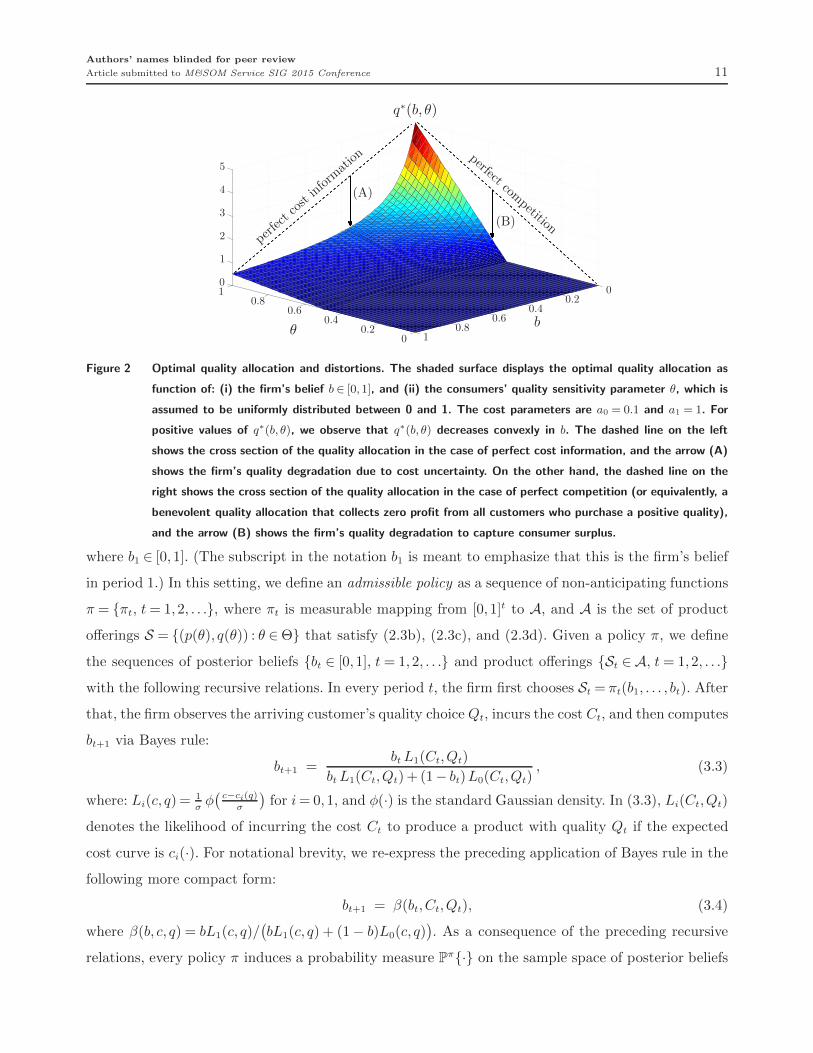
Figure 2 displays an optimal quality allocation example, in which the customers’ quality sensitivity

parameters are distributed uniformly on the unit interval. The two quality degradation effects men-

tioned above are shown as arrows (A) and (B). The monopoly distortion effect in (B) vanishes at the

upper boundary of Θ = [0,1], whereas the uncertainty distortion effect in (A) attains its maximum

value at the upper boundary of Θ = [0,1], leading to significant quality degradation at intermediate

belief levels that are away from 0 or 1.

3. Dynamic Learning about Cost Uncertainty

In this section, we extend the original problem formulation in the preceding section to the case where

the firm dynamically learns about the underlying cost curve. Suppose that the firm now sells its

products over T sales periods, where each sales period entails a learning opportunity about costs. In

every period t= 1,2, . . . , T , the firm first chooses a product offering St = {(pt(θ), qt(θ)) : θ ∈ Θ}, which

is a set of price-quality pairs to be offered to its customers. After that, a customer whose quality

sensitivity θt is randomly drawn from the density f(·) arrives and selects a price-quality pair from

the firm’s product offering St (or the outside option of zero net utility). Let Qt = qt(θt) denote the

quality choice of the customer arriving in period t. Following a sale, the firm incurs the following cost

of production:

Ct = c(Qt) + ǫt for t= 1,2, . . . , (3.1)

where c(·) is underlying cost curve which is unknown to the firm, and ǫtiid∼ N (0, σ2) are idiosyncratic

cost shocks of consumers.

To formally define dynamic pricing-and-quality-allocation policies in this framework, let us first

recall the firm’s prior belief, which was originally expressed in (2.2):

c(·) =

{c1(·) with probability b1

c0(·) with probability 1 − b1,(3.2)



θb

q∗(b, θ)

00.2

0.40.6

0.81 0

0.20.4

0.60.8

1

0

1

2

3

4

5

perfe

ctco

stinform

ation perfect com

petition

(A)

(B)

Figure 2 Optimal quality allocation and distortions. The shaded surface displays the optimal quality allocation as

function of: (i) the firm’s belief b ∈ [0,1], and (ii) the consumers’ quality sensitivity parameter θ, which is

assumed to be uniformly distributed between 0 and 1. The cost parameters are a0 = 0.1 and a1 = 1. For

positive values of q∗(b, θ), we observe that q∗(b, θ) decreases convexly in b. The dashed line on the left

shows the cross section of the quality allocation in the case of perfect cost information, and the arrow (A)

shows the firm’s quality degradation due to cost uncertainty. On the other hand, the dashed line on the

right shows the cross section of the quality allocation in the case of perfect competition (or equivalently, a

benevolent quality allocation that collects zero profit from all customers who purchase a positive quality),

and the arrow (B) shows the firm’s quality degradation to capture consumer surplus.

where b1 ∈ [0,1]. (The subscript in the notation b1 is meant to emphasize that this is the firm’s belief

in period 1.) In this setting, we define an admissible policy as a sequence of non-anticipating functions

π = {πt, t= 1,2, . . .}, where πt is measurable mapping from [0,1]t to A, and A is the set of product

offerings S = {(p(θ), q(θ)) : θ ∈ Θ} that satisfy (2.3b), (2.3c), and (2.3d). Given a policy π, we define

the sequences of posterior beliefs {bt ∈ [0,1], t= 1,2, . . .} and product offerings {St ∈ A, t= 1,2, . . .}with the following recursive relations. In every period t, the firm first chooses St = πt(b1, . . . , bt). After

that, the firm observes the arriving customer’s quality choiceQt, incurs the cost Ct, and then computes

bt+1 via Bayes rule:

bt+1 =btL1(Ct,Qt)

btL1(Ct,Qt) + (1 − bt)L0(Ct,Qt), (3.3)

where: Li(c, q) = 1σφ(

c−ci(q)

σ

)for i= 0,1, and φ(·) is the standard Gaussian density. In (3.3), Li(Ct,Qt)

denotes the likelihood of incurring the cost Ct to produce a product with quality Qt if the expected

cost curve is ci(·). For notational brevity, we re-express the preceding application of Bayes rule in the

following more compact form:

bt+1 = β(bt,Ct,Qt), (3.4)

where β(b, c, q) = bL1(c, q)/(bL1(c, q) + (1 − b)L0(c, q)

). As a consequence of the preceding recursive

relations, every policy π induces a probability measure Pπ{·} on the sample space of posterior beliefs



[0,1]T . To construct this probability measure, let us define the following transition density for beliefs:

ψS(x, y) = x

∫

Θ

∫

{γ∈R :β(x,γ,q(θ))=y}L1

(γ, q(θ)

)f(θ)dγ dθ

+(1 −x)

∫

Θ

∫

{γ∈R :β(x,γ,q(θ))=y}L0

(γ, q(θ)

)f(θ)dγ dθ (3.5)

for all x, y ∈ [0,1] and S ∈ A, where q(·) is the quality allocation function in the product offering S.

Because the transition density ψS(x, y) depends only on the quality allocation q(·) in S, we will also

use the equivalent notation ψq(·)(x, y) = ψS(x, y) when necessary. Thus, given the value of b1 = b, Pπ{·}is defined by the following relations: Pπ{b1 = b} = 1, and

Pπ{bt+1 ∈ dy | b1, . . . , bt} = ψS(bt, y)dy (3.6)

for all t= 1,2, . . . , T , and y ∈ [0,1].

The firm’s objective is to choose an admissible policy to maximize its expected profit over T periods.

For brevity, let r(b,S) be the firm’s expected single-period profit, expressed as a function of the firm’s

belief b and product offering S = {(p(θ), q(θ)) : θ ∈ Θ} ∈ A; i.e.,

r(b,S) :=

∫

Θ

(p(θ) −C

(b, q(θ)

))f(θ)dθ (3.7)

for b∈ [0,1] and S ∈ A. To maximize the expected over T periods, the firm solves

maxπ∈Π

Eπ

{T∑

t=1

r(bt,St)

∣∣∣∣b1 = b

}, (3.8)

where b∈ [0,1], Π is the set of all admissible policies, and Eπ{·} is the expectation operator associated

with Pπ{·}. We hereafter refer to the problem in (3.8) as the dynamic learning problem. Our next

result constructs the optimal value function for the dynamic learning problem and the associated

optimal policy.

Proposition 4. (optimal value function and optimal policy)

(i) (existence) There exists a unique sequence of functions {Vn(·), n= 0,1, . . . , T} that satisfy

Vn(x) = maxS∈A

{r(x,S) +

∫ 1

0

Vn−1(y)ψS(x, y)dy

}for x∈ [0,1] and n= 1, . . . , T, (3.9a)

V0(x) = 0 for x∈ [0,1]. (3.9b)

(ii) (verification) VT (·) satisfies VT (x) ≥ maxπ∈Π Eπ{∑T

t=1 r(bt,St)∣∣ b1 = x

}for x∈ [0,1].

(iii) (attainment) Let π∗ be an admissible policy satisfying π∗t (b1, . . . , bt) = ϕT−t+1(bt), where

ϕn(x) := argmaxS∈A

{r(x,S) +

∫ 1

0

Vn−1(y)ψS(x, y)dy

}(3.10)

for x∈ [0,1] and n= 1, . . . , T . Then,

Eπ∗{

T∑

t=1

r(bt,S∗t )

∣∣∣∣b1 = x

}= VT (x) for x∈ [0,1], (3.11)

where {S∗t , t= 1,2, . . .} is the sequence of product offerings under policy π∗.



Proposition 4 shows that the optimal value function for the firm’s dynamic learning problem is

characterized by the recursive relation in (3.9a), which is usually referred to as the Bellman equation,

and the boundary condition in (3.9b). More importantly, this result verifies that the optimal value is

attained by a Markovian policy that uses only the firm’s most recent belief to determine the product

offering in a given period. We will now analyze the Bellman equation in detail to gain further insights

into the structure of the optimal value function and the optimal policy. By Proposition 1, we know

that the quality allocation function qt(·) must be increasing and differentiable almost everywhere to

induce IC and IR in period t. Moreover, as argued in the derivation of (2.4) in the preceding section,

the pricing function in period t, namely pt(·), satisfies the following relation to induce IC and IR:

pt(θ) = θqt(θ) −∫ θ

θmin

qt(ξ)dξ for all θ ∈ Θ. (3.12)

Given the above structure for the pricing function pt(·), we note that the product offering in period t,

namely St, is completely characterized by its quality allocation function qt(·). Consequently, we can

re-express the Bellman equation in (3.9a) as follows:

Vn(b) = maxq(·)∈A∗

{∫ θmax

θmin

(θq(θ) −

∫ θ

θmin

q(ξ)dξ−C(x, q(θ)

))f(θ)dθ+

∫ 1

0

Vn−1(y)ψq(·)(b, y)dy

}

for all b ∈ [0,1] and n= 1, . . . , T , where A∗ is the set of functions q : Θ → R+ that are increasing and

differentiable almost everywhere. Recalling the definition of the transition density for beliefs in (3.5),

we further obtain


{∫ θmax

θmin

(θq(θ) −

∫ θ

θmin


))f(θ)dθ

+ b

∫ θmax

θmin

( ∫ ∞

−∞Vn−1

(β(b, γ, q(θ)

))L1

(γ, q(θ)

)dγ

)f(θ)dθ

+(1 − b)

∫ θmax

θmin

( ∫ ∞

−∞Vn−1

(β(b, γ, q(θ)

))L0

(γ, q(θ)

)dγ

)f(θ)dθ

}(3.13)

for all b ∈ [0,1] and n = 1, . . . , T . Noting that all of the three integrals on the right hand side of

(3.13) have the common domain of [θmin, θmax], we can simplify (3.13) by introducing the following

conditional value function:

Vn(b, q) := b

∫ ∞

−∞Vn

(β(b, γ, q)

)L1(γ, q)dγ+(1 − b)

∫ ∞

−∞Vn

(β(b, γ, q)

)L0(γ, q)dγ (3.14)

for all b ∈ [0,1], q ∈ Q, and n = 0,1, . . . , T . The value of Vn(b, q) corresponds to the firm’s optimal

profit-to-go in the remaining n periods, conditional on the firm selling a product of quality q. Using

this definition of the conditional value function, we express (3.13) as


{∫ θmax

θmin

(θq(θ) −

∫ θ

θmin


)+Vn−1

(b, q(θ)

))f(θ)dθ

}(3.15)



for all b ∈ [0,1] and n= 1, . . . , T . As argued in the derivation of (2.6), we use integration by parts to

deduce that∫ θ

θminq(ξ)dξ=F (θ)q(θ)/f(θ), which further simplifies (3.15) to the following:


{∫ θmax

θmin

(θq(θ) − F (θ)

f(θ)q(θ) −C

(b, q(θ)

)+Vn−1

(b, q(θ)

))f(θ)dθ

}(3.16)

for all b∈ [0,1] and n= 1, . . . , T . Let q∗n(b, θ) be optimal quality allocation for the problem in (3.16); i.e.,

q∗n(b, ·) := argmax

q(·)∈A∗

{∫ θmax

θmin

(θq(θ) − F (θ)

f(θ)q(θ) −C

(b, q(θ)

)+Vn−1

(b, q(θ)

))f(θ)dθ

}(3.17)

for all b∈ [0,1] and n= 1, . . . , T .

As in Section 2, we will measure the inefficiency due to cost uncertainty by comparing the firm’s

performance with the performance of a clairvoyant who knows the underlying cost structure. To that

end, let us first generalize the definitions of the firm’s loss and quality degradation functions, which

were originally expressed in (2.8) and (2.9) respectively. Define

∆n(b) := bVn(1) + (1 − b)Vn(0) −Vn(b) for all b∈ [0,1] and n= 1, . . . , T, (3.18)

δn(b, θ) := bq∗n(1, θ) + (1 − b)q∗

n(0, θ) − q∗n(b, θ) for all b∈ [0,1], θ ∈ Θ, and n= 1, . . . , T. (3.19)

Note that the functions V1(b), ∆1(b), q∗1(b, θ), and δ1(b, θ) in the above definitions correspond to

V (b), ∆(b), q∗(b, θ), and δ(b, θ), respectively, analyzed in Section 2. For the definition of quality

degradation in (3.19), readers are reminded that positive (negative) values of δn(b, θ) correspond to

quality decreases (increases) relative to the expected quality allocation with perfect cost information.

In the next proposition, we show that the firm’s n-period loss due to cost uncertainty, namely ∆n(b),

is increasing in n.

Proposition 5. (monotonicity of firm’s loss due to uncertainty) ∆n+1(b) ≥ ∆n(b) for all

b∈ [0,1] and n= 1, . . . , T − 1.

Using Proposition 5, we obtain the following result:

Proposition 6. (firm’s loss due to uncertainty) ∆n(b) is concave, and there exists a finite

positive constant K such that ∆n(b) ≥Kb(1 − b) ≥ 0 for all b∈ [0,1] and n= 1, . . . , T .

Propositions 5 and 6 extend Propositon 3 in Section 2 by establishing that the firm’s loss in the

n-period dynamic learning problem increases with n and attains larger values for intermediate values

of the firm’s belief b. Figure 3 shows this behavior of ∆n(b).

The preceding results in this section show that the profit implications of static cost uncertainty,

which was analyzed in Section 2, also hold in the case of dynamic learning. But, the opportunity

of dynamic learning has a contrasting effect on the firm’s optimal quality allocation. The quality

distortion due to uncertainty, which was established in Theorem 1, is mitigated in the dynamic learning

problem. To show the extent of this mitigation we present the next two results:



b

∆n(b)

0 0.2 0.4 0.6 0.8 10

0.5

1.0

1.5

n= 1n= 1n= 1n= 1

n= 5n= 5n= 5n= 5

n= 10n= 10n= 10n= 10

n= 20n= 20n= 20n= 20

Figure 3 Firm’s loss due to uncertainty in the dynamic learning problem. The loss ∆n(b) is increasing in n, and is

concave in b. The consumers’ quality sensitivity parameters are uniformly distributed between 0 and 1. The

cost parameters are a0 = 0.1 and a1 = 1.

Theorem 2. (uniform quality improvement for learning) Let b ∈ [0,1] and n ≥ 2. Then,

δn(b, θ) ≤ δ1(b, θ) for all θ ∈ Θ.

Theorem 2 states that, in the dynamic learning problem, the quality distortion due to uncertainty

is mitigated for all types of customers, implying that the opportunity of learning about the cost

structure improves quality uniformly for all potential customers. The main reason behind this result

is that selling the product at a higher quality provides a clearer signal about the underlying cost

curve; hence the firm can use quality improvements as a tool to accelerate its learning. Consequently,

the firm chooses to increase the quality of its product offering to eliminate future losses due to cost

uncertainty. A key feature of Theorem 2 is that the aforementioned quality improvement is offered

to every customer, establishing that learning is valuable even when the firm’s expected profit is

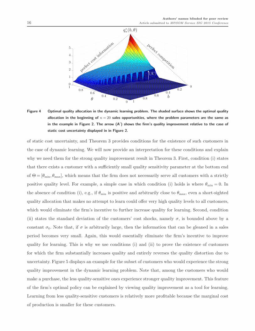
conditioned upon the quality sensitivity of an arriving customer. Figure 4 displays the optimal quality

allocation function q∗n(b, θ) in a numerical example of the dynamic learning problem.

In our next result we prove that, in the dynamic learning problem, the quality degradation result

in Theorem 1 is entirely reversed for a subset of customers.

Theorem 3. (strong quality improvement for learning) Let b ∈ (0,1), n ≥ 2, and assume

that: (i) θmin ≤ 1/f(θmin), and (ii) σ≤ σ0 where σ0 is a finite positive constant. Then, there exists an

open set Eb,n ⊆ Θ of strictly positive measure such that δn(b, θ)< 0 for all θ ∈Eb,n.

While the uniform quality improvement result in Theorem 2 prescribes higher quality levels for all

types of customers, such quality improvements cannot be arbitrarily large because a sufficiently large

quality improvement for all customers would lead to a net loss almost surely; i.e., the firm’s n-period

profit would be negative under both of the possible cost curves c0(·) and c1(·). It is therefore important

to understand if there exist customers who should be offered quality levels higher than the expected

clairvoyant quality allocation. By Theorem 1 we know that there exist no such customers in the case



θb

q∗n(b, θ)

00.2

0.40.6

0.81 0

0.20.4

0.60.8

1

0

1

2

3

4

5

perfe

ctco

stinform

ation perfect com

petition

(A′)

Figure 4 Optimal quality allocation in the dynamic learning problem. The shaded surface shows the optimal quality

allocation in the beginning of n = 20 sales opportunities, where the problem parameters are the same as

in the example in Figure 2. The arrow (A′) shows the firm’s quality improvement relative to the case of

static cost uncertainty displayed in in Figure 2.

of static cost uncertainty, and Theorem 3 provides conditions for the existence of such customers in

the case of dynamic learning. We will now provide an interpretation for these conditions and explain

why we need them for the strong quality improvement result in Theorem 3. First, condition (i) states

that there exists a customer with a sufficiently small quality sensitivity parameter at the bottom end

of Θ = [θmin, θmax], which means that the firm does not necessarily serve all customers with a strictly

positive quality level. For example, a simple case in which condition (i) holds is where θmin = 0. In

the absence of condition (i), e.g., if θmin is positive and arbitrarily close to θmax, even a short-sighted

quality allocation that makes no attempt to learn could offer very high quality levels to all customers,

which would eliminate the firm’s incentive to further increase quality for learning. Second, condition

(ii) states the standard deviation of the customers’ cost shocks, namely σ, is bounded above by a

constant σ0. Note that, if σ is arbitrarily large, then the information that can be gleaned in a sales

period becomes very small. Again, this would essentially eliminate the firm’s incentive to improve

quality for learning. This is why we use conditions (i) and (ii) to prove the existence of customers

for which the firm substantially increases quality and entirely reverses the quality distortion due to

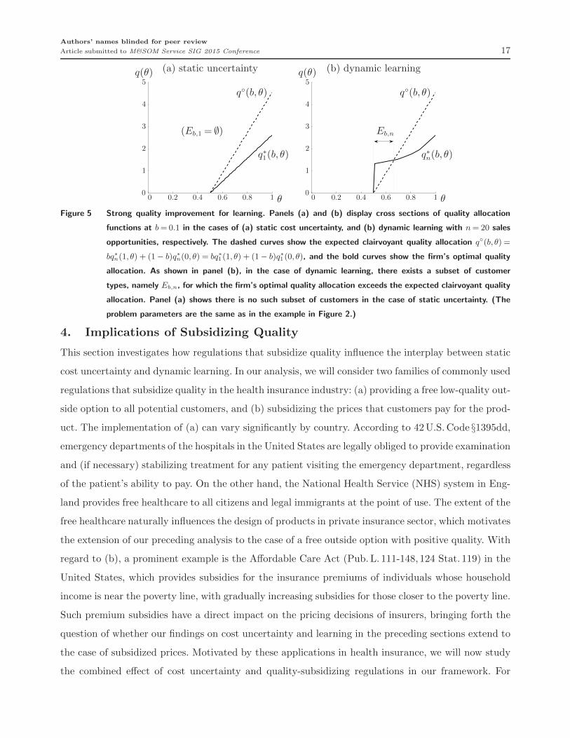
uncertainty. Figure 5 displays an example for the subset of customers who would experience the strong

quality improvement in the dynamic learning problem. Note that, among the customers who would

make a purchase, the less quality-sensitive ones experience stronger quality improvement. This feature

of the firm’s optimal policy can be explained by viewing quality improvement as a tool for learning.

Learning from less quality-sensitive customers is relatively more profitable because the marginal cost

of production is smaller for these customers.



θ

q(θ) (a) static uncertainty

θ

q(θ) (b) dynamic learning

00 0.20.2 0.40.4 0.60.6 0.80.8 1100

11

22

33

44

55

(Eb,1 = ∅)

q∗1(b, θ)

q◦(b, θ)

Eb,n

q∗n(b, θ)

q◦(b, θ)

Figure 5 Strong quality improvement for learning. Panels (a) and (b) display cross sections of quality allocation

functions at b = 0.1 in the cases of (a) static cost uncertainty, and (b) dynamic learning with n = 20 sales

opportunities, respectively. The dashed curves show the expected clairvoyant quality allocation q◦(b, θ) =

bq∗n(1, θ) + (1 − b)q∗

n(0, θ) = bq∗1(1, θ) + (1 − b)q∗

1(0, θ), and the bold curves show the firm’s optimal quality

allocation. As shown in panel (b), in the case of dynamic learning, there exists a subset of customer

types, namely Eb,n, for which the firm’s optimal quality allocation exceeds the expected clairvoyant quality

allocation. Panel (a) shows there is no such subset of customers in the case of static uncertainty. (The

problem parameters are the same as in the example in Figure 2.)

4. Implications of Subsidizing Quality

This section investigates how regulations that subsidize quality influence the interplay between static

cost uncertainty and dynamic learning. In our analysis, we will consider two families of commonly used

regulations that subsidize quality in the health insurance industry: (a) providing a free low-quality out-

side option to all potential customers, and (b) subsidizing the prices that customers pay for the prod-

uct. The implementation of (a) can vary significantly by country. According to 42U.S. Code §1395dd,

emergency departments of the hospitals in the United States are legally obliged to provide examination

and (if necessary) stabilizing treatment for any patient visiting the emergency department, regardless

of the patient’s ability to pay. On the other hand, the National Health Service (NHS) system in Eng-

land provides free healthcare to all citizens and legal immigrants at the point of use. The extent of the

free healthcare naturally influences the design of products in private insurance sector, which motivates

the extension of our preceding analysis to the case of a free outside option with positive quality. With

regard to (b), a prominent example is the Affordable Care Act (Pub. L. 111-148, 124 Stat. 119) in the

United States, which provides subsidies for the insurance premiums of individuals whose household

income is near the poverty line, with gradually increasing subsidies for those closer to the poverty line.

Such premium subsidies have a direct impact on the pricing decisions of insurers, bringing forth the

question of whether our findings on cost uncertainty and learning in the preceding sections extend to

the case of subsidized prices. Motivated by these applications in health insurance, we will now study

the combined effect of cost uncertainty and quality-subsidizing regulations in our framework. For



both (a) and (b), we will begin with verifying the implementability of the regulation, which includes

deriving conditions for incentive compatibility and individual rationality in product design, as well

as investigating whether the regulation in question can be implemented as a welfare-increasing reg-

ulation. That is, for both (a) and (b), we will show the existence of quality-subsidizing regulations

that can increase social welfare, relative to the case of no regulation. After that, we will generalize

our results on cost uncertainty and learning in Sections 2 and 3 to the cases of quality-subsidizing

regulations.

4.1. Free Low-quality Outside Option

Suppose that every potential customer has the outside option of obtaining a product with quality

q0 > 0 at zero price. Let us first consider how the presence of this outside option will affect the firm’s

pricing and quality allocation decisions. As in our analysis of the original problem in Section 2, the

firm’s optimal product offering S = {(p(θ), q(θ)) : θ ∈ Θ} prescribes a threshold θc ∈ [θmin, θmax) such

that the customers whose quality sensitivities are greater than θc will be served with a positive quality

allocation. But this time, the outside option is more attractive; hence θc could be higher relative to

the original problem. (Note that, in both cases, θc could be equal to θmin if θmin is sufficiently high.) To

emphasize the critical threshold θc in the firm’s product offering, we can express the firm’s problem

with the free outside option of quality q0 as follows:

V f(b, q0) = maxp(·),q(·)

{∫ θmax

θc

(p(θ) −C

(b, q(θ)

))f(θ)dθ

}(4.1a)

s.t. θq(θ) − p(θ) ≥ θq(θ) − p(θ) for all θ, θ ∈ [θc, θmax], (4.1b)

θq(θ) − p(θ) ≥ θq0 for all θ ∈ [θc, θmax], (4.1c)

q(θ) ≥ 0 for all θ ∈ [θc, θmax]. (4.1d)

We note that our original problem in (2.3) is a special case of (4.1) with q0 = 0, which implies that

V f(b,0) = V (b). The distinguishing feature of the preceding problem is the net utility of the free

outside option, θq0, which appears on the right hand side of the IR constraints (4.1c). To normalize

the customers’ utility curves, let us define the firm’s excess quality allocation function:

x(θ) := q(θ) − q0 for all θ ∈ [θc, θmax]. (4.2)

Using the definition of x(·), we obtain the following counterpart of Proposition 1.

Proposition 7. (incentive compatibility and individual rationality)

(i) The IC constraints (4.1b) hold if and only if x(·) is increasing and differentiable almost every-

where, and p′(θ) = θx′(θ) for θ ∈ Θ, except on a set of measure zero.

(ii) Assume that the IC constraints (4.1b) hold, and that θc x(θc)−p(θc) = 0. Then the IR constraints

(4.1c) also hold.



As argued in (2.4), Proposition 7 implies that

p(θ) = θx(θ) −∫ θ

θc

x(ξ)dξ for all θ ∈ [θc, θmax]. (4.3)

Therefore, by the arguments used to derive (2.6), the firm’s problem becomes

V f(b, q0) = maxx(·)∈A∗

{∫ θmax

θc

(θx(θ) − F (θ)

f(θ)x(θ) −C

(b, q0 +x(θ)

))f(θ)dθ

}(4.4)

for all b ∈ [0,1] and q0 ≥ 0, where A∗ is the set of functions x : [θc, θmax] → R+ that are increasing

and differentiable almost everywhere. Let qf(b, θ, q0) be the firm’s optimal quality allocation for the

problem in (4.4). That is, qf(b, θ, q0) = q0 +xf(b, θ, q0), where

xf(b, ·, q0) = argmaxx(·)∈A∗

{∫ θmax

θc

(θx(θ) − F (θ)

f(θ)x(θ) −C

(b, q0 +x(θ)

))f(θ)dθ

}. (4.5)

Figure 6 shows a plot of qf(b, θ, q0) in a numerical example. Note that the critical threshold θc, over

which the firm’s quality allocation is preferred to the outside option, varies over different values of

the firm’s belief b. In particular, as the firm’s belief on the higher cost curve c1(·) increases, the firm

chooses to serve a smaller set of potential customers.

θb

qf(b, θ, q0)

00.2

0.40.6

0.81 0

0.20.4

0.60.8

1

0

1

2

3

4

5

Figure 6 Optimal quality allocation with free low-quality outside option. The shaded surface shows the firm’s optimal

quality allocation in presence of a free outside option of quality q0 = 0.15. (The rest of the problem

parameters are the same as in the example in Figure 2.)

Our next goal is to verify that a free outside option can be implemented as a welfare-increasing

regulation. To that end, let q(b, θ, q0) be the quality level that a customer with sensitivity parameter

θ would receive when the firm’s belief is b and the quality of the free outside option is q0; i.e.,

q(b, θ, q0) =

{q0 if θ≤ θf

c(b, q0)

qf(b, θ, q0) otherwise,(4.6)



where θfc(b, q0) = inf

{θ ∈ [θmin, θmax] : x

f(b, θ, q0) ≥ 0}

is the critical threshold over which the firm offers

its customers a quality that is preferred to the outside option. Then, the social welfare with the free

outside option of quality q0 is

W f(b, q0) =

∫ θmax

θmin

(θq(b, θ, q0) −C

(b, q(b, θ, q0)

))f(θ)dθ. (4.7)

In the original problem in (2.3), we have q0 = 0, and hence the social welfare in that case is

W (b) = W f(b,0) =

∫ θmax

θmin

(θq∗(b, θ) −C

(b, q∗(b, θ)

))f(θ)dθ. (4.8)

Our next result shows that the presence of a free outside option can increase social welfare.

Proposition 8. (welfare impact of free low-quality outside option) There exists a finite

and positive constant κ such that, if 0< q0 ≤ κ, then W f(b, q0)>W (b) for all b∈ [0,1].

The preceding proposition establishes that a free outside option can increase social welfare as long

as the quality of the outside option is positive and sufficiently small. As seen on Figure 7, the social

welfare function W f(b, q0) is increasing in q0 for smaller values of q0 and becomes decreasing in q0

when the value of q0 becomes excessively large. The main reason for this behavior is that, for large

values of q0, the outside option simply provides a very high quality whose marginal cost exceeds its

marginal benefit to society, resulting in a net decrease of social welfare.

q0

W f(b, q0)

0 0.1 0.2 0.3 0.40.10

0.11

0.12

0.13

0.14

Figure 7 Social welfare with free low-quality outside option. The social welfare with a free outside option of quality

q0, namely W f(b, q0), is increasing in q0 for sufficiently small values of q0. The firm’s prior belief is b = 0.5,

and the problem parameters are the same as in the example in Figure 2.

Having shown that a free low-quality outside option can be implemented as a welfare-increasing

regulation, our next goal is to study its impact on the quality distortion due to uncertainty. Given

that the customers now receive qualities according to (4.6), we modify the definition of our quality

degradation function in (2.9) as follows:

δf(b, θ, q0) := bq(1, θ, q0) + (1 − b)q(0, θ, q0) − q(b, θ, q0) for all b∈ [0,1], θ ∈ Θ, and q0 > 0. (4.9)

Note that δf(b, θ, q0) accounts for the fact that customers that are not served by the firm receive the

quality of q0. Our next result characterizes how a free outside option with positive quality moderates

the quality degradation due to uncertainty.



Theorem 4. (quality degradation due to uncertainty) Let q0 > 0.

(i) There exists an increasing function g : Θ → R+ such that g(θmax)> 0 and δf(b, θ, q0) ≥ g(θ)b(1−b) ≥ 0 for b∈ [0,1] and θ ∈

[θf

c(1, q0), θmax

].

(ii) There exists an open set E ⊆ [0,1]×[θf

c(0, q0), θfc(1, q0)

]such that δf(b, θ, q0)< 0 for (b, θ) ∈E.

Remark The function g(·) that appears in part (i) of the above theorem is the same function g(·) in

Theorem 1.

Theorem 4 describes in two parts the combined effect of the cost uncertainty and the free outside

option with positive quality. Part (i) establishes that, in the presence of a free outside option with

positive quality, the quality distortion result in Theorem 1 is preserved for customers that are highly

sensitive to quality. On the other hand, part (ii) shows that we can have mixed results for lower

levels of quality sensitivity; in particular, the firm’s optimal quality allocation can exceed the expected

clairvoyant quality allocation.

b

qf(b, θℓ, q0)(a) low θ

b

qf(b, θh, q0)(b) high θ

00 0.20.2 0.40.4 0.60.6 0.80.8 1100

0.50.5

1.01.0

1.51.5

2.02.0

2.52.5

Figure 8 Quality degradation with free low-quality option. The bold curves in panels (a) and (b) show cross sections

of the quality allocation function qf(b, θ, q0) for θℓ = 0.745 and θh = 0.755 respectively, where: q0 = 0.25,

the consumers’ quality sensitivity parameters are uniformly distributed between 0 and 1, and the cost

parameters are a0 = 0.1 and a1 = 0.5. The dashed curves show the expected clairvoyant quality allocation

in each case. Panel (a) shows that qf(b, θ, q0) can exceed the expected clairvoyant quality allocation for

small values of θ, whereas panel (b) shows that the quality degradation due to uncertainty will almost

surely affect top consumers.

Figure 8 displays a numerical example regarding the two parts of Theorem 4. As shown in Figure

8(b), the customers with sufficiently high θ never prefer the outside option, and the convexity of the

firm’s optimal quality allocation leads to a distortion similar to the one we established in Theorem 1.

However, the customers with relatively lower values of θ might have to purchase the low-quality outside

option if the underlying cost curve happens to be the larger one, which means that the clairvoyant

quality allocation for these customers would be q0 if c(·) = c1(·). Consequently, as shown in Figure

8(a), the firm’s uncertainty about the cost curve might result in a better quality allocation than the

expected clairvoyant quality allocation for customers with relatively lower quality sensitivity.



4.2. Price Subsidy

Suppose that a regulatory authority subsidizes a fraction of the price that a customer pays for the

product. For a customer with quality sensitivity parameter θ, let τ(θ) ∈ [0,1] denote the unsubsidized

fraction of the price. That is, a customer with quality sensitivity θ pays only τ(θ)p to purchase the

product at price p, and the remainder of the price, namely(1− τ(θ)

)p, is subsidized. In this case, the

net utility of purchasing a product with quality q at price p becomes

U s(θ, q, p) = θq− τ(θ)p , (4.10)

where θ ∈ Θ is the quality sensitivity of the purchasing customer. Consequently, the firm’s problem

with subsidized prices can be expressed as follows:

V s(b, τ) = maxp(·),q(·)

{∫ θmax

θmin

(p(θ) −C

(b, q(θ)

))f(θ)dθ

}(4.11a)

s.t. θq(θ) − τ(θ)p(θ) ≥ θq(θ) − τ(θ)p(θ) for all θ, θ ∈ Θ, (4.11b)

θq(θ) − τ(θ)p(θ) ≥ 0 for all θ ∈ Θ, (4.11c)

q(θ) ≥ 0 for all θ ∈ Θ. (4.11d)

Letting 1(·) denote the constant function that maps Θ to {1}, we note that the original problem

formulation in (2.3) is a special case of (4.11) with τ = 1. Thus, V s(b,1) = V (b).

Our first goal is to find necessary and sufficient conditions for IC and IR when prices are subsidized.

For that purpose, let us define a feasible set for the function τ . Let T be the set of functions τ : Θ →(0,1] that are increasing, concave, and differentiable almost everywhere. In Figure 9, we display a

piecewise linear subsidization scheme τ ∈ T .

θ

τ(θ)

0 0.2 0.4 0.6 0.8 10

0.2

0.4

0.6

0.8

1

Figure 9 Price subsidization example. Customers with θ ≤ 0.4 pay only a fraction of the price, whereas the remaining

customers pay the full price.

In the next result, we extend Proposition 1 to the case of subsidized prices.

Proposition 9. (incentive compatibility and individual rationality) Let τ ∈ T . Then the

following statements hold:

(i) The IC constraints (4.11b) hold if and only if q(·) is increasing and differentiable almost every-

where, and τ(θ)p′(θ) = θq′(θ) for θ ∈ Θ, except on a set of measure zero.



(ii) Assume that the IC constraints (4.11b) hold, and that θmin q(θmin)− τ(θmin)p(θmin) = 0. Then the

IR constraints (4.11c) also hold.

Using Proposition 9 and integrating by parts, we deduce that the pricing function p(·) must satisfy

the following to induce IC and IR:

p(θ) = ν(θ)q(θ) −∫ θ

θmin

ν ′(ξ)q(ξ)dξ for all θ ∈ Θ, (4.12)

where ν(θ) := θ/τ(θ). Here, ν(θ) can be interpreted as the effective quality sensitivity of a customer

under the price subsidization scheme τ . Recalling the arguments we used for deriving (2.6), we can

re-express the firm’s problem in (4.11) as follows:

V s(b, τ) = maxq(·)∈A∗

{∫ θmax

θmin

(ν(θ)q(θ) − F (θ)

f(θ)ν ′(θ)q(θ) −C

(b, q(θ)

))f(θ)dθ

}(4.13)

for all b ∈ [0,1] and τ ∈ T , where A∗ is the set of functions q : Θ → R+ that are increasing and

differentiable almost everywhere. Denote by qs(b, θ, τ) the firm’s optimal quality allocation for the

problem in (4.13); i.e.,

qs(b, ·, τ) = argmaxq(·)∈A∗

{∫ θmax

θmin

(ν(θ)q(θ) − F (θ)

f(θ)ν ′(θ)q(θ) −C

(b, q(θ)

))f(θ)dθ

}. (4.14)

As in the preceding subsection, we will first verify that a price subsidy can be implemented as a

welfare-increasing regulation. Under the quality allocation qs(b, θ, τ), the social welfare is

W s(b, τ) =

∫ θmax

θmin

(θqs(b, θ, τ) −C

(b, qs(b, θ, τ)

))f(θ)dθ. (4.15)

The following proposition shows that there exists a function τ under which W s(b, τ) achieves its

highest possible value over all feasible quality allocations.

Proposition 10. (welfare impact of price subsidy) Let τ∗(θ) = θF (θ)/(∫ θmax

θξf(ξ)dξ

)for

all θ ∈ Θ. Then,

W s(b, τ∗) = maxq(·)∈A∗

{∫ θmax

θmin

(θq(θ) −C

(b, q(θ)

))f(θ)dθ

}≥ W (b) for all b∈ [0,1]. (4.16)

Proposition 10 explicitly characterizes a price subsidization scheme τ∗ that induces the firm to choose

a welfare-maximizing quality allocation, which is usually referred to as the first best solution. (Figure

10 displays τ∗ in a numerical example.) Naturally, the existence of τ∗ implies that a price subsidy can

be implemented as a welfare-increasing regulation. To derive the subsidization formula in Proposition

10, we solve an ordinary differential equation that ensures that the firm’s marginal revenue for serving

a customer with quality sensitivity θ is equal to the marginal social benefit of serving this customer.

Once this relationship is established, the firm simply chooses its product offering to maximize social

welfare.



θ

τ∗(θ)

0 0.2 0.4 0.6 0.8 10

0.2

0.4

0.6

0.8

1

Figure 10 Welfare-maximizing price subsidization. The function τ∗ increases concavely on Θ = [0,1]. The consumers’

quality sensitivity parameters are uniformly distributed over Θ.

Finally, we focus on whether the firm exercises any quality degradation in its product offering in

the presence of both price subsidies and cost uncertainty. To that end, define

δs(b, θ, τ) := bqs(1, θ, τ) + (1 − b)qs(0, θ, τ) − qs(b, θ, τ) for all b∈ [0,1], θ ∈ Θ, and τ ∈ T . (4.17)

The last result of this subsection shows that the quality distortion due to uncertainty persists under

price subsidies.

Theorem 5. (quality degradation due to uncertainty) Let τ ∈ T . Then there exists an

increasing function G : Θ → R+ such that G(θmax)> 0 and δs(b, θ, τ) ≥G(θ)b(1− b) ≥ 0 for all b∈ [0,1]

and θ ∈ Θ.

The preceding theorem states that, even if welfare-maximizing subsidization schemes such as τ∗

are implemented, a firm facing uncertainty about its cost curve would still degrade the quality of its

products, relative to the expected clairvoyant quality allocation. Figure 11 demonstrates this behavior

of the firm in a numerical example.

θb

qs(b, θ, τ∗)

00.2

0.40.6

0.81 0

0.20.4

0.60.8

1

0

1

2

3

4

5

perfe

ctco

stinform

ation perfect com

petition

Figure 11 Optimal quality allocation with price subsidy. The shaded surface shows the firm’s optimal quality alloca-

tion qs(b, θ, τ∗) under the welfare-maximizing price subsidization scheme τ∗. While the monopoly distortion

effect disappears under τ∗, the uncertainty distortion effect is still present in qs(b, θ, τ∗). (The problem

parameters are the same as in the example in Figure 2.)



4.3. Dynamic Learning in Presence of Quality Subsidization

This subsection extends our findings on dynamic learning in Section 3 to the case of quality-subsidizing

regulations. To generalize the basic problem formulation, we first consider the case of a free outside

option with positive quality, and let rf(b,S, q0) denote the firm’s single-period profit, expressed as a

function of the firm’s belief b, product offering S = {(p(θ), q(θ)) : θ ∈ Θ}, and the quality of the free

outside option q0. Similarly, in the case of price subsidies, let rs(b,S, τ) be the firm’s single-period

profit as a function of the firm’s belief b, product offering S, and the subsidization scheme τ . Under

both subsidization schemes, the firm can make observations on its cost curve as explained in (3.1),

and we construct admissible policies in a non-anticipating fashion such that the product offering in a

given period t= 1, . . . , T depends only on past observations. As a result, the firm solves the following

multi-period problems under quality-subsidizing regulations:

V fn(b, q0) := max

π∈ΠEπ

{n∑

t=1

rf(bt,St, q0)

∣∣∣∣b1 = b

}for b∈ [0,1], q0 > 0, and n= 1, . . . , T, (4.18)

V sn(b, τ) := max

π∈ΠEπ

{n∑

t=1

rs(bt,St, τ)

∣∣∣∣b1 = b

}for b∈ [0,1], τ ∈ T , and n= 1, . . . , T, (4.19)

where Π is the set of all admissible policies. The problem in (4.18) corresponds to the case of a free

outside option with positive quality q0, while the problem in (4.19) corresponds to the case of price

subsidization scheme τ . Let qfn(b, θ, q0) and qs

n(b, θ, τ) be the firm’s optimal quality allocation functions

in the first sales period of the problems in (4.18) and (4.19), respectively. Then, we can extend the

definition of the quality degradation functions in (3.19) as follows:

δfn(b, θ, q0) := bqf

n(1, θ, q0) + (1 − b)qfn(0, θ, q0) − qf

n(b, θ, q0) (4.20)

δsn(b, θ, τ) := bqs

n(1, θ, τ) + (1 − b)qsn(0, θ, τ) − qs

n(b, θ, τ) (4.21)

for all b∈ [0,1], q0 > 0, τ ∈ T , and n= 1, . . . , T . The following theorem extends Theorem 2 by showing

that, under quality subsidization, the firm uniformly improves the quality in its product offering to

accelerate its learning.

Theorem 6. (uniform quality improvement for learning) Let b ∈ [0,1], n ≥ 2, q0 > 0, and

τ ∈ T . Then, δfn(b, θ, q0) ≤ δf

1(b, θ, q0) and δsn(b, θ, τ) ≤ δs

1(b, θ, τ) for all θ ∈ Θ.

5. Extensions and Concluding Remarks

In this last section, we discuss possible extensions of our analysis.

Batch arrivals of customers. In many practical applications of dynamic pricing, firms might not

necessarily be able to adjust their product offerings after every sales opportunity. To accommodate

such cases in our analysis, let us consider an extension of our model where the firm makes multiple

observations on the cost curve before the product offering can be changed. Suppose that, in every



period t, N distinct customers arrive. The firm observes their quality choices {Qjt, j = 1, . . . ,N}, and

incurs the production costs {Cjt, j = 1, . . . ,N} to serve these customers, where Cjt = c(Qjt)+ ǫjt , and

ǫjtiid∼ N (0, σ2). To extend our analysis to this case, we replace the belief updating equation in (3.3)

with the following: The firm’s posterior belief in period t+1 is given by

bt+1 =bt

∏N

j=1L1(Cjt,Qjt)

bt∏N

j=1L1(Cjt,Qjt) + (1 − bt)∏N

j=1L0(Cjt,Qjt), (5.1)


c−ci(q)

σ

)for i = 0,1, and φ(·) is the standard Gaussian density. Redefining the

transition density for beliefs in (3.5) based on (5.1), the firm’s optimal policy in this modified dynamic

learning problem can be constructed as in Section 3. We note that this modification of the dynamic

learning problem can be viewed as a more constrained version of our original problem in Sections 2

and 3, where the added constraint is that the firm is allowed to use its most recent beliefs only in

periods t∈ {1, N+1, 2N+1, . . .}. Consequently, the optimal policy in this extension is a feasible (but

not necessarily optimal) policy in our original problem. Therefore, the firm’s loss due to uncertainty

would increase in this extension, relative to our setting. More importantly, to reflect the value of

learning in its quality allocation, the firm would still need to improve quality, but because every sales

period provides a larger amount of information, the firm would have to make more drastic innovations

in its product offering after every batch of observations.

Generalizing the belief distribution on cost uncertainty. In this paper, we have modeled

the firm’s uncertainty about costs using two cost hypotheses. That is, the firm has a Bernoulli belief

distribution on two possible cost curves. To extend this model to more general prior beliefs, suppose

that the firm has a belief distribution on M +1 possible cost curves. That is, the firm initially believes

that c(·) = ci(·) with probability bi,1 for i= 0,1, . . . ,M , where∑M

i=0 bi,1 = 1, ci(q) = aiq2 for all q ∈ Q,

and 0< a0 < · · ·< aM <∞. Let bt = (bi,t, i= 0,1, . . . ,M) be the firm’s belief vector in period t. Then,

the firm’s belief updating equation to compute bt+1 becomes

bi,t+1 =bi,tLi(Ct,Qt)∑M

i=0 bi,tLi(Ct,Qt)for i= 0,1, . . . ,M, (5.2)


c−ci(q)

σ

)for i= 0,1, . . . ,M , and φ(·) is the standard Gaussian density. Using (5.2),

we can extend the definition of the transition density in (3.5) to the case of belief vectors, and then

construct the corresponding optimal policy as in Section 3. A key issue in this construction is that the

generalized dynamic programming problem has a higher dimensional state space, which might involve

computational challenges for large values of M . To establish the value of learning in this case, one

needs to prove the convexity of the value function associated the with generalized dynamic learning

problem (i.e., the firm should find the expected clairvoyant profit more valuable than its optimal profit



as function of the belief vector). For that purpose, we note that our proof of the convexity of the

value function uses the linearity of the expected profit with respect to bt, which remains valid in this

generalization. Because learning is still valuable in the generalized version of our dynamic learning

problem, one would expect that the firm needs to improve quality for learning purposes.

When the firm has a belief distribution on a multitude of cost curves, it is possible that the extreme

cost scenarios in the firm’s belief distribution could be drastically different from each other, thereby

exacerbating the uncertainty in the firm’s business environment. A key issue in this context is to

provide the firm the right incentives to mitigate some of the quality distortion due to uncertainty.

In health insurance practice, this can be achieved by covering the firm’s additional cost under a

high-cost scenario while charging a fee under a low-cost scenario (see, e.g., the risk corridors of the

ACA, Goodell 2014). In our setting, this effectively eliminates some of the possible cost scenarios,

resulting in a belief distribution concentrated on a smaller number of cost hypotheses. If a regulatory

authority implements a stabilization scheme to eliminate the extreme cost curves, then the differences

between the clairvoyant quality allocations for the worst and best cost scenarios would be reduced.

As a result, under such an stabilization scheme, one would expect to see a smaller quality distortion

due to uncertainty.

Time-varying customer population. Our model assumes that the distribution of customers’

quality sensitivity parameters θ has a fairly general density f(θ), but this density remains the same

over time. In the health insurance context, which serves as our motivation, a key issue is the aging pop-

ulation of potential customers. In particular, as the customer population gets older, one might expect

that their medical needs would increase, thereby raising the quality-sensitivity of customers. To gain

insights into this case, we can consider a time-varying modification of our model: Let the distribution

of θ in period t be a uniform distribution between 0 and θmax(t), and assume that {θmax(t), t= 1,2, . . .}evolves according to the following equation:

θmax(t+1) = A(θmax(t)

)for t= 1,2, . . . , (5.3)

where A : R → R is an increasing function, and θmax(1) is a positive constant. In this case, the firm’s

dynamic learning problem in (3.8) would be replaced by

maxπ∈Π

Eπ

{T∑

t=1

rt(bt,St)

∣∣∣∣ b1 = b

}, (5.4)

where rt(b,S) is the firm’s single-period profit function for period t. The distinguishing feature of the

problem in (5.4) is that the single-period profit function is now dependent on period t. Because the

firm’s customer population is spread to larger intervals in later periods, the firm would be able to

screen its infinitesimal customers in a finer way as t increases, meaning that r∗t (b) ≤ r∗

t+1(b) where



r∗t (b) = maxS∈A{rt(b,S)}. As a result, later periods would provide more lucrative sales opportunities

to the firm; hence, one would expect to see a more pronounced quality improvement for learning.

Cost-heterogeneity of customers. In our model, we considered a cost curve that is characterized

by the product quality; hence the firm’s production costs depend indirectly on the quality-sensitivities

of customers. If the customers’ quality-sensitivities are known to have a direct and heterogeneous

effect on production costs, we can extend our model to accommodate this case as follows. Let us

replace ci(q), i= 0,1, with the two-dimensional cost curves ci(θ, q) = ai(θ)q2, i= 0,1, where a0(·) and

a1(·) are functions from Θ to R++ such that a0(θ)< a1(θ) for all θ ∈ Θ. In this case, the firm’s problem

with static cost uncertainty, which was originally expressed in (2.7), becomes

maxq(·)∈A∗

{∫ θmax

θmin

(θq(θ) − F (θ)

f(θ)q(θ) −C

(b, θ, q(θ)

))f(θ)dθ

}, (5.5)

where C(b, θ, q) = bc1(θ, q)+(1−b)c0(θ, q), and A∗ is the set of functions q : Θ → R+ that are increasing

and differentiable almost everywhere. Letting q∗(b, θ) be the optimal quality allocation for the problem

in (5.5), we note that the proof of Theorem 1 is valid in this extension, with the exception that the

function g(·) in the quality distortion lower bound in Theorem 1 is replaced by

g(θ) =

(a1(θ) − a0(θ)

)2(θ−F (θ)/f(θ)

)+

2a0(θ)a21(θ)

. (5.6)

Because g(θ) is positive for all θ ∈ Θ, one would still observe a quality degradation due to uncertainty

in this extension. Interestingly, this suggests that the firm would degrade the quality further for the

customers whose quality sensitivity θ increases the difference a1(θ)−a0(θ); i.e., the customers who are

expected to incur substantially different costs under the hypotheses {c= c0} and {c= c1} would face

more quality distortion. From a practical standpoint, this means that if a regulation or technological

innovation significantly affects a particular region in the domain of the firm’s cost curve c(θ, q), then

the heterogenous cost parameters under the two hypotheses, namely a0(θ) and a1(θ), would differ

substantially and result in stronger quality distortion over the affected region.

Health-contingent wellness programs and moral hazard. In the broader context of health

insurance, a related issue is the implementation of health-contingent wellness programs, which can

help an insurer partially control its customers’ cost shocks. The Affordable Care Act allows certain

insurers to implement health-contingent wellness programs to induce healthier customer behavior (see,

e.g., Health Care Reform Bulletin 2013). One of the goals of such wellness programs is to mitigate the

moral hazard that emerges when a customer decides to exploit a high-quality product after the time of

sales, resulting in increased subsequent costs for the firm’s higher quality products. To explicitly model

the role of a customer’s unobservable effort that can avoid cost inflation after the time of sales, one can

consider the following extension of our setting. After a sale in period t, the firm makes multiple cost



observations that involve a sequence of cost shocks {ǫs,t, s= 1,2, . . . , S} in (3.1), such that each shock

ǫs,t depends on a subsequent effort process {es ∈ [emin, emax], s= 1, . . . , S}, which is to be determined

by the customer. To be precise, we let ǫs,t = µ(es) + ξs,t for all s= 1, . . . , S, where µ : [emin, emax] → R

is a decreasing function with µ(emin) > 0 and µ(emax) = 0, and ξs,t are independent and identically

distributed random variables with mean zero and variance σ2. If it is costly for customers to exert an

effort greater than emin, then the firm would need to incentivize its customers to reduce after-sales

costs using rewards and penalties adapted to the idiosyncratic cost observations from a customer. Our

basic model can be viewed as the case where the firm induces the customers to exert a fixed effort

level es = e∗ for all s= 1,2, . . . , S such that the expected cost due to moral hazard is minimized.

More on regulations: Funding and labor supply. In Section 4, we have studied how commonly

used quality-subsidizing regulations affect the firm’s price and quality decisions. It is worth noting

that two additional questions in the implementation of these regulations are: how they should be

funded, and how they will influence the labor supply. For the former question, we note that both of

the regulations we have studied can be funded by allocating taxes on the firm and the customers. A

free low-quality outside option decreases the firm’s profits, and hence needs to be funded by customers

who receive larger amounts of net utility. On the other hand, price subsidies increase the firm’s profits,

and hence can be funded by the firm in a Pareto-efficient way. Regarding the latter question, if we

view the firm as an employer that provides health insurance to its employees, then the customers

who obtain a positive utility from the firm’s products constitute the firm’s labor supply. With this

interpretation in mind, the two aforementioned regulations have contrasting effects on labor supply:

While the free low-quality outside option decreases labor supply, the price subsidies increase it (see

Garthwaite, Gross and Notowidigdo 2014, for further discussion of the relationship between health

insurance regulations and labor supply).

A. Proof of Propositions 2-3 and Theorem 1

Proof of Proposition 2. Let us first characterize the optimal solution of (2.7). Note that we can maximize

the integral in (2.7) by choosing the quality q(θ) to maximize the integrand for each value of θ. Therefore, the

first order necessary conditions for (unconstrained) optimality are as follows:

θ− F (θ)

f(θ)=

∂C(b, q(θ)

)

∂qfor all θ ∈ Θ. (A.1)

Because C(b, q) = bc1(q) + (1 − b)c0(q) = ba1q2 + (1 − b)a0q

2, the preceding conditions are equivalent to θ −F (θ)/f(θ) = 2ba1q(θ)+2(1−b)a0q(θ) for all θ ∈ Θ. Since C(b, q) is convex in q, we know that the above necessary

conditions are also sufficient for optimality. Recalling that f(θ) has increasing failure rate, we deduce that

F (θ)/f(θ) is decreasing in θ, and hence the solution to (A.1) is increasing in θ, satisfying the monotonicty

constraint for q(·). Therefore, the optimal quality allocation q∗(b, θ) for the problem in (2.7) is given by

q∗(b, θ) =

(θ−F (θ)/f(θ)

2a0 + 2(a1 − a0)b

)

+

for all b∈ [0,1] and θ ∈ Θ, (A.2)



where x+ = max{x,0} for all x ∈ R. Note that, if q∗(b, θ) is an interior solution, then ∂q∗(b, θ)/∂b = −(θ −

F (θ)/f(θ))(a1 − a0)/

(2a0 + 2(a1 − a0)b

)2< 0 and ∂2q∗(b, θ)/∂b2 = 2

(θ − F (θ)/f(θ)

)(a1 − a0)

2/(2a0 + 2(a1 −

a0)b)3> 0. As a result, in any open subset of [0,1] × Θ in which q∗(b, θ) is an interior solution, q∗(b, θ) is a

strictly decreasing and strictly convex function of b.

Proof of Proposition 3. Let θc = inf{θ ∈ [θmin, θmax] : θ−F (θ)/f(θ) ≥ 0

}. Let b ∈ [0,1]. Because q∗(b, θ) = 0

for all θ≤ θc, we have

V (b) =

∫ θmax

θc

(θq∗(b, θ)− F (θ)

f(θ)q∗(b, θ)−C

(b, q∗(b, θ)

))f(θ)dθ

(b)=

κ

a0 + (a1 − a0)b, (A.3)

where κ= 14

∫ θmax

θc

(θ−F (θ)/f(θ)

)2f(θ)dθ, and (b) follows by (A.2). Using the preceding identity and elementary

algebra, we consequently get

∆(b) =bκ

a1

+(1 − b)κ

a0

− κ

a0 + (a1 − a0)b≥ (a1 − a0)

2κb(1 − b)

a0a21

= Kb(1 − b), (A.4)

where K = (a1 − a0)2κ/(a0a

21).

Proof of Theorem 1. Note that

δ(b, θ) = bq∗(1, θ)+ (1 − b)q∗(0, θ)− q∗(b, θ)(a)= g0(θ)

(b

a1

+1 − b

a0

− 1

a0 + (a1 − a0)b

)(b)

≥ g0(θ)(a1 − a0)2b(1 − b)

a0a21

for all b∈ [0,1] and θ ∈ Θ, where: g0(θ) = 12

(θ−F (θ)/f(θ)

)+, (a) follows by (A.2), and (b) follows by the argument

used to derive (A.4). Therefore, letting g(θ) = g0(θ)(a1 −a0)2/(a0a

21), we deduce that δ(b, θ) ≥ g(θ)b(1−b) for all

b∈ [0,1] and θ ∈ Θ. Since f(θ) has increasing failure rate, g(θ) is increasing in θ. Moreover, because F (θmax) = 0

and θmax > 0, we have g(θmax)> 0.

B. Proof of Theorem 2

Step 1: Prove that ∂Vn(b, q)/∂q≥ 0 for all b∈ [0,1], and q ∈ Q. Fix b ∈ [0,1], q ∈ Q, and n ≥ 2. Let us first

express the marginal conditional value function in the following lemma.

Lemma 1. (derivative of conditional value function)

∂Vn(b, q)

∂q= b

∫ ∞

−∞Vn

(β(b, γ, q)

)s(γ, q)L1(γ, q)dγ+ (1 − b)

∫ ∞

−∞Vn

(β(b, γ, q)

)s(γ, q)L0(γ, q)dγ (B.1)

for all b∈ [0,1], and q ∈ Q, where s(γ, q) := 2q−1(σ−2(γ− a0q

2)(γ− a1q2)− 1

).

Note that, in the integrands on the right hand side of (B.1), almost all terms are non-negative; the only term

with a mixed sign is s(γ, q). To be more precise, the function s(·, q) is a parabola with the following roots:

γ0 =(a0 + a1)q

2 −√

(a1 − a0)2q4 + 4σ2

2and γ1 =

(a0 + a1)q2 +

√(a1 − a0)2q4 + 4σ2

2. (B.2)

Thus,

s(γ, q)

{< 0 if γ ∈ (γ0, γ1)

≥ 0 otherwise.(B.3)

Let xi = β(b, γi, q) and yi = Vn(xi) for i= 0,1. Because β(b, γ, q) is increasing in γ, we know that

β(b, γ, q) ≤ x0 if and only if γ ≤ γ0 ;

β(b, γ, q) ∈ (x0, x1) if and only if γ ∈ (γ0, γ1) ;

β(b, γ, q) ≥ x1 if and only if γ ≥ γ1 . (B.4)

Now, define a function h : [0,1] → R such that h(b) = m0 + m1b, where m0 = y0x1 − y1x0 and m1 = (y0 −y1)/(x0 − x1). That is, h(·) is the affine function whose trajectory coincides with the line passing through the



points (x0, y0) and (x1, y1). Because Vn(·) is a convex function, Vn(b) ≤ h(b) if b ∈ (x0, x1), and Vn(b) ≥ h(b) if

b∈ (−∞, x0] ∪ [x1,∞). Consequently, we deduce from (B.4) that

Vn

(β(b, γ, q)

)− h

(β(b, γ, q)

)≥ 0 if and only if γ ≤ γ0 ;

Vn

(β(b, γ, q)

)− h

(β(b, γ, q)

)≤ 0 if and only if γ ∈ [γ0, γ1] ;

Vn

(β(b, γ, q)

)− h

(β(b, γ, q)

)≥ 0 if and only if γ ≥ γ1 . (B.5)

Recalling (B.3), we deduce that(Vn

(β(b, γ, q)

)− h

(β(b, γ, q)

))s(γ, q) ≥ 0 for all γ ∈ R. This implies that

0 ≤ b

∫ ∞

−∞

(Vn

(β(b, γ, q)

)− h

(β(b, γ, q)

))s(γ, q)L1(γ, q)dγ+ (1 − b)

∫ ∞

−∞

(Vn

(β(b, γ, q)

)− h

(β(b, γ, q)

))s(γ, q)L0(γ, q)dγ

(a)=

∂Vn(b, q)

∂q− b

∫ ∞

−∞h(β(b, γ, q)

)s(γ, q)L1(γ, q)dγ− (1 − b)

∫ ∞

−∞h(β(b, γ, q)

)s(γ, q)L0(γ, q)dγ, (B.6)

where (a) follows by Lemma 1. To eliminate the remaining integrals on the right hand side of (B.6), we state

another lemma.

Lemma 2. Let h : [0,1] → R be an affine function. Then,

0 = b

∫ ∞

−∞h(β(b, γ, q)

)s(γ, q)L1(γ, q)dγ+ (1 − b)

∫ ∞

−∞h(β(b, γ, q)

)s(γ, q)L0(γ, q)dγ (B.7)

for all b∈ [0,1], and q ∈ Q.

By Lemma 2, the right hand side of (B.6) is equal to ∂Vn(b, q)/∂q, from which we conclude that ∂Vn(b, q)/∂q≥ 0.

Step 2: Prove that q∗n(b, θ) ≥ q∗

1(b, θ) for n≥ 2. Fix b∈ [0,1]. By (3.17), we know that

q∗n(b, ·) = argmax

q(·)∈A∗

{∫ θmax

θmin

(R(θ)q(θ)− ab

(q(θ)

)2+ Vn−1

(b, q(θ)

))f(θ)dθ

}, (B.8)

where R(θ) = θ−F (θ)/f(θ) and ab = ba1 +(1− b)a0. As argued in the proof of Proposition 2, we can maximize

the integral in (B.8) by maximizing its integrand for every θ ∈ Θ, and the (unconstrained) maximizer satisfies

the following first order necessary condition:

Ψn(b, θ, q) := R(θ)− 2abq+∂Vn−1

(b, q

)

∂q= 0. (B.9)

Consider the first order condition for n = 1; in this case, we have Vn−1(b, q) = V0(b, q) = 0 for all q ∈ Q, and

hence ∂V0(b, q)/∂q = 0 for all q ∈ Q. Let θc = inf{θ ∈ Θ :R(θ) ≥ 0

}. For all θ ≤ θc, we have q∗

1(b, θ) = 0, which

implies that q∗n(b, θ) ≥ q∗

1(b, θ). For all θ > θc, we have q∗1(b, θ) = R(θ)/(2ab), and hence R(θ) − 2abq ≥ 0 for

all q ∈ [0, q∗1(b, θ)]. Now, let n≥ 2. Because ∂Vn−1(b, q)/∂q ≥ 0 as shown in Step 1, Ψn(b, θ, q) = R(θ) − 2abq+

∂Vn−1

(b, q

)/∂q≥ 0 for all q ∈ [0, q∗

1(b, θ)]. This means that the maximizer that satisfies the first order condition

for n≥ 2, namely q∗n(b, θ), is greater than or equal to q∗

1(b, θ). As a result, q∗n(b, θ) ≥ q∗

1(b, θ) for θ ∈ Θ and n≥ 2.

Step 3: Prove that δn(b, θ) ≤ δ1(b, θ) for n≥ 2. Fix b∈ [0,1], θ ∈ Θ, and n≥ 2. Note that

∂Vn(i, q)

∂q

(b)= i

∫ ∞

−∞Vn

(β(i, γ, q)

)s(γ, q)L1(γ, q)dγ+ (1 − i)

∫ ∞

−∞Vn

(β(i, γ, q)

)s(γ, q)L0(γ, q)dγ

(c)= i Vn(i)

∫ ∞

−∞s(γ, q)L1(γ, q)dγ+ (1 − i)Vn(i)

∫ ∞

−∞s(γ, q)L0(γ, q)dγ

(d)= 0 (B.10)

for i= 0,1, and q ∈ Q, where: (b) follows by Lemma 1; (c) follows because β(i, γ, q) = i for i∈ {0,1}, γ ∈ R, and

q ∈ Q; and (d) follows by Lemma 2 and the fact that a constant function is affine. Therefore, q∗n(i, θ) = q∗

1(i, θ)

for i= 0,1, implying that δn(b, θ) ≤ δ1(b, θ).

References

Araman, V. and Caldentey, R. (2009), ‘Dynamic Pricing for Nonperishable Products with Demand Learning’, Operations

Research 57(5), 1169–1188.



Aviv, Y. and Pazgal, A. (2005), ‘A Partially Observed Markov Decision Process for Dynamic Pricing’, Management

Science 51(9), 1400–1416.

Bergemann, D., Shen, J., Xu, Y. and Yeh, E. (2012), ‘Mechanism Design with Limited Information: The Case of Nonlinear

Pricing’, Game Theory for Networks pp. 1–10.

Bergemann, D. and Valimaki, J. (2000), ‘Experimentation in markets’, The Review of Economic Studies 67(2), 213–234.

Besanko, D., Donnenfeld, S. and White, L. (1987), ‘Monopoly and Quality Distortion: Effects and Remedies’, The

Quarterly Journal of Economics 102(4), 743–768.

Besanko, D., Donnenfeld, S. and White, L. (1988), ‘The Multiproduct Firm, Quality Choice, and Regulation’, The Journal

of Industrial Economics 36(4), 411–429.

den Boer, A. (2014), ‘Dynamic Pricing with Multiple Products and Partially Specified Demand Distribution’, Mathematics

of Operations Research 39(3), 863–888.

Farias, V. and van Roy, B. (2010), ‘Dynamic Pricing with a Prior on Market Response’, Operations Research 58(1), 16–29.

Garthwaite, C., Gross, T. and Notowidigdo, M. (2014), ‘Public Health Insurance, Labor Supply, and Employment Lock’,

Quarterly Journal of Economics 129(2), 653–696.

Goodell, S. (2014), ‘Health Policy Brief: Risk Corridors’. Health Affairs, June 26, 2014.

Goodnough, A. (2014), ‘Newly Insured, Many Now Face Learning Curve’. The New York Times, Published on August

3, 2014, p. A1. URL: http://nyti.ms/1m9Xr71.

Harrison, J., Keskin, N. and Zeevi, A. (2012), ‘Bayesian Dynamic Pricing Policies: Learning and Earning Under a Binary

Prior Distribution’, Management Science 58(3), 570–586.

Health Care Reform Bulletin (2013), ‘Wellness Program Final Rules Increase Maximum Rewards, but Include Significant

New Requirements’. Towers Watson, June 11, 2013.

Jullien, B. (2000), ‘Participation Constraints in Adverse Selection Models’, Journal of Economic Theory 93, 1–47.

Keller, G. and Rady, S. (1999), ‘Optimal Experimentation in a Changing Environment’, The Review of Economic Studies

66(3), 475–507.

Keller, G. and Rady, S. (2003), ‘Price Dispersion and Learning in a Dynamic Differentiated-Goods Duopoly’, RAND

Journal of Economics 34(1), 138–165.

Keskin, N. and Zeevi, A. (2014), ‘Dynamic Pricing with an Unknown Demand Model: Asymptotically Optimal Semi-

myopic Policies’, Operations Research 62(5), 1142–1167.

Kowalski, A. (2014), ‘The Early Impact of the Affordable Care Act’. Working Paper, Yale University, New Haven, CT.

Lippman, S. and McCardle, K. (1987), ‘Does Cheaper, Faster, or Better Imply Sooner in the Timing of Innovation

Decisions?’, Management Science 33(8), 1058–1064.

Maskin, E. and Riley, J. (1984), ‘Monopoly with Incomplete Information’, The RAND Journal of Economics 15(2), 171–

196.

Mazzola, J. and McCardle, K. (1996), ‘A Bayesian Approach to Managing Learning-curve Uncertainty’, Management

Science 42(5), 680–692.

McCardle, K. (1985), ‘Information Acquisition and the Adoption of New Technology’, Management Science 31(11), 1372–

1389.

Mussa, M. and Rosen, S. (1978), ‘Monopoly and Product Quality’, Journal of Economic Theory 18(2), 301–317.

Rochet, J. and Stole, L. (2002), ‘Nonlinear Pricing with Random Participation’, The Review of Economic Studies 69, 277–

311.

Smith, J. and Ulu, C. (2012), ‘Technology Adoption with Uncertain Future Costs and Quality’, Operations Research

60(2), 262–274.

Ulu, C. and Smith, J. (2009), ‘Uncertainty, Information Acquisition, and Technology Adoption’, Operations Research

57(3), 740–752.

Documents

Dynamic Pricing and Product Di erentiation with Cost