Introduction to UnconventionalSuperconductivity

Manfred Sigrist

Theoretische Physik, ETH-Hönggerberg, 8093 Zürich, Switzerland

Abstract. This lecture gives a basic introduction into some aspects ofthe unconventional supercon-ductivity. First we analyze the conditions to realized unconventional superconductivity in stronglycorrelated electron systems. Then an introduction of the generalized BCS theory is given and sev-eral key properties of unconventional pairing states are discussed. The phenomenological treatmentbased on the Ginzburg-Landau formulations provides a view on unconventional superconductivitybased on the concept of symmetry breaking. Finally some aspects of two examples will be discussed:high-temperature superconductivity and spin-triplet superconductivity in Sr2RuO4.

Keywords: Unconventional superconductivity, high-temperature superconductivity, Sr2RuO4

INTRODUCTION

Superconductivity remains to be one of the most fascinatingand intriguing phases ofmatter even nearly hundred years after its first observation. Owing to the breakthrough in1957 by Bardeen, Cooper and Schrieffer we understand superconductivity as a conden-sate of electron pairs, so-called Cooper pairs, which form due to an attractive interactionamong electrons. In the superconducting materials known until the mid-seventies thisinteraction is mediated by electron-phonon coupling whichgises rise to Cooper pairs inthe most symmetric form, i.e. vanishing relative orbital angular momentum and spin sin-glet configuration (nowadays calleds-wave pairing). After the introduction of the BCSconcept, also studies of alternative pairing forms started. Early on Anderson and Morel[1] as well as Balian and Werthamer [2] investigated superconducting phases which laterwould be identified as the A- and the B-phase of superfluid3He [3]. In contrast to thes-wave superconductors the A- and B-phase are characterizedby Cooper pairs with an-gular momentum 1 and spin-triplet configuration. This was the beginning of the era ofunconventionalsuperconductivity, condensates of Cooper pairs of lower symmetry, incontrast to theconventionalsuperconductors with the most symmetric Cooper pairs.

The discovery of superfluidity in the3He in 1971 by Osheroff, Richardson and Leegave the first example of unconventional Cooper pairing [4].In 3He other pairing mecha-nisms are obviously of non-phononic origin, based on van derWaals and spin fluctuationmediated interactions [3, 5]. Moreover,3He is the prime example for a strongly corre-lated Fermi liquid where the short range repulsive interaction leads to strong renormal-isations of the quasiparticle mass and other quantities. Alternative pairing mechanismand strong correlation effects are key elements to prevent electrons from undergoingconventionals-wave pairing.

The natural aim to find among solids a system with unconventional Cooper pairingwas not satisfied until much latter when at the end of seventies and beginning of the

eighties two novel classes of strongly correlated materials were found among whichsome were superconducting - the heavy Fermion compounds [6,7, 8] and organic con-ductors [9, 10]. The first type of materials are intermetallics containing rare earth ionsand the second are highly anisotropic conductors based organic units. Although it is notclear until today which form of Cooper pairing is realized inmany of these materials,some of them possess complex phase diagrams with several different superconductingphases, firmly establishing the unconventional nature. In both types of material super-conductivity emerges out of phase that are nearly magnetic or evolve under pressurefrom a magnetically ordered state. In 1986 the discovery of high-temperature supercon-ductivity in cuprate compounds with layered perovskite structure announced the era ofunconventional superconductivity to a wider community [11]. This system dominates tothe present days the study of superconductivity. A few yearswere necessary to estab-lish the unconventional character to pairing for the cuprates. Cooper pairs possess in thequasi-two-dimensional systems a so-called spin singletdx2−y2-wave structure [12, 13].In cuprate materials the important role of magnetism in the context of the unusual metal-lic properties and superconductivity is underlined by the fact that this superconductoremerges from an antiferromagnetic Mott-insulator upon carrier doping [14].

The essential role which magnetism could play for unconventional superconductivitybecame one of the guiding strategies in the nineties in the search for new materials.Striking examples of superconductivity associated with magnetic phases are several Ce-based compounds where superconductivity is associated with a quantum critical pointof an antiferromagnetically ordered phase. CeIn3 [15], CePd2Si2 [15, 16] and CeMIn5(M=Co,Rh,Ir) [17, 18] are a few examples of this type. Surprisingly superconductivitywas also found inside a ferromagnetic phases in UGe2 [19], URhGe [20] and ZrZn2 [21],possibly connected with the corresponding magnetic quantum phase transition.

Sr2RuO4 whose superconductivity was discovered in 1994 deserves a special placeas an exemplary case of an unconventional superconductor resulting from a stronglycorrelated Fermi liquid phase [22]. In various respects it may be considered as an analogto 3He, including the pairing symmetry which is closely relatedto the A-phase of thesuperfluid. Many aspects of this superconductor have been explored in much detailduring the last ten years [23, 24]

More recently the superconducting skutterudites such as PrOs4Sb12 have beenaroused much interest as new examples of heavy Fermion materials with multiplesuperconducting phases [25]. The exploration of superconductivity in materials withgeometrically frustrated crystall lattices has been a further recent focus. This in-cludes NaxCoO4 intercalated with water which has been considered as a realizationof superconductivity on a triangular lattice [26]. Also superconductivity in metallswith the pyrochlor structure belong to this class such as Cd2Re2O7 [27] and AOs2O6(A=Cs,Rb,K) [28], although it is not clear whether they are unconventional. Crystalstructure can have an even crucial impact on superconductivity than in the case offrustrated lattices, if inversion symmetry is missing. As we will see later inversiontogether with time reversal invariance are among the key symmetries for Cooper pairformation. The discovery of superconductivity in the heavyFermion systems CePt3Siand UIr have reopened the discussion of superconductivity in this kind of systems [29].

During the past two decades we experience important developments in the field ofunconventional superconductivity, from the side of new materials as well as theoretical

understanding. New strategies for the discovery of unconventional superconductors bearfruits besides the tremendous progress in sample production which is a mandatoryaccessory for the observation of unconventional superconducting phases which arevery sensitive to material disorder effects. These lecturenotes cover a few aspects anddevelopments in the field of unconventional superconductivity. Naturally this overviewis selective and the viewpoint is biased by the preferences of the lecturer.

CONVENTIONAL VERSUS UNCONVENTIONALSUPERCONDUCTIVITY

The most fundamental experimental aspect of superconductivity is the screening of amagnetic field, the Meissner-Ochsenfeld effect, which implies also the existence of per-sistent electric currents. The microscopic theory which provides such a feature is basedon the coherent state introduced by Bardeen, Cooper and Schrieffer. In this chapter wewill give a brief introduction to this BCS state (screening effects, however, will be onlyaddressed later in the context of the phenomenological Ginzburg-Landau formulation)and motivate the generalization beyond the standard BCS theory of conventional super-conductivity. We will compare also the electron-phonon mechanism for superconduc-tivity with possible alternative mechanisms, in particular, based on effective interactionoriginating from spin fluctuations.

Standard BCS theory

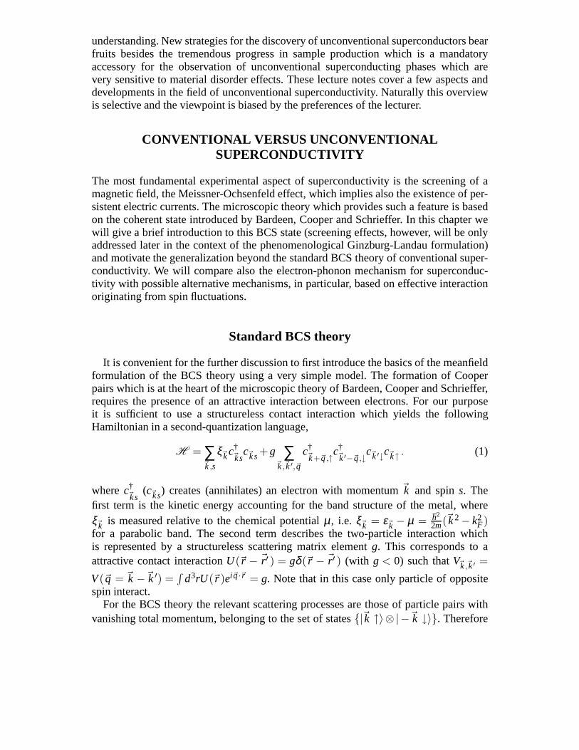
It is convenient for the further discussion to first introduce the basics of the meanfieldformulation of the BCS theory using a very simple model. The formation of Cooperpairs which is at the heart of the microscopic theory of Bardeen, Cooper and Schrieffer,requires the presence of an attractive interaction betweenelectrons. For our purposeit is sufficient to use a structureless contact interaction which yields the followingHamiltonian in a second-quantization language,

H = ∑~k,s

ξ~kc†~ks

c~ks+g ∑~k,~k ′,~q

c†~k+~q,↑c

†~k ′−~q,↓c~k ′↓c~k↑ . (1)

wherec†~ks

(c~ks) creates (annihilates) an electron with momentum~k and spins. Thefirst term is the kinetic energy accounting for the band structure of the metal, whereξ~k is measured relative to the chemical potentialµ, i.e. ξ~k = ε~k − µ = h2

2m(~k2− k2F)

for a parabolic band. The second term describes the two-particle interaction whichis represented by a structureless scattering matrix element g. This corresponds to aattractive contact interactionU(~r − ~r ′ ) = gδ (~r − ~r ′ ) (with g < 0) such thatV~k,~k′ =

V(~q = ~k −~k ′) =∫

d3rU (~r )ei~q·~r = g. Note that in this case only particle of oppositespin interact.

For the BCS theory the relevant scattering processes are those of particle pairs withvanishing total momentum, belonging to the set of states|~k ↑〉⊗ |−~k ↓〉. Therefore

we concentrate on the reduced Hamiltonian

H = ∑~k,s

ξ~kc†~ks

c~ks+g ∑~k,~k ′

c†~k↑c

†−~k↓c−~k ′↓c~k ′↑ . (2)

ignoring all other pair scattering events. Bardeen, Cooperand Schrieffer introduced thefollowing variational ground state

|ΦBCS〉 = ∏~k

u~k +v~kc†

~k↑c†−~k↓

|vac〉 (3)

where|vac〉 denotes the electron vacuum (|u~k |2+ |v~k |2 = 1). This is a coherent states ofelectron pairs (Cooper pairs) giving a lower energy than thebare Fermi gas.

An alternative approach which provides also straightforwardly the quasiparticle spec-trum of the coherent state is given by the mean field theory which allows us to reducethe interaction part. Among the possible meanfields we use the off-diagonal

b~k =⟨

c−~k↓c~k↑

⟩(4)

which connects states of particle numbers different by 2, assuggested by the variationalstate (3). Note that the expectation value〈A〉 = tr[exp(−βH )A]/tr[exp(−βH )]. Wemay interpretb~k as the wavefunction of the Cooper pairs in momentum space. Insertingc−~k↓c~k↑ = b~k +c−~k↓c~k↑−b~k into the Hamiltonian and neglecting terms quadratic in

. . . (we assume〈|. . .|2〉 |b~k |2) we obtain the meanfield Hamiltonian

H = ∑~k,s

ξ~kc†~ks

c~ks+g ∑~k,~k ′

b∗~k ′c−~k↓c~k↑ +b~k ′c†~k↑c

†−~k↓−b∗~kb~k ′ (5)

= ∑~k,s

ξ~kc†~ks

c~ks−∑~k

(∆∗c−~k↓c~k↑ +∆c†

~k↑c†−~k↓

)−∆∗b~k (6)

with ∆ = −g∑~k′ b~k ′. It is now straightforward to find the quasiparticle spectrum of thisone-particle Hamiltonian by introducing new Fermion operators γ~ks with the property

γ†~ks

= i[Hm f,γ†~ks

] = E~kγ†~ks

. To reach such a diagonalization of the Hamiltonian we usethe Bogolyubov transformation

c~k↑ = u∗~kγ~k1 +v~kγ†~k2

and c−~k↓ = −v∗~kγ~k1 +u~kγ†~k2

(7)

with∣∣u~k

∣∣2 +∣∣v~k∣∣2 = 1 and indices 1 and 2 stands for the electron like and hole like

quasiparticle. Note that the functionsu~k andv~k are identical with those of the variationalstate (3). The Hamiltonian acquires the diagonal form

Hm f = ∑~k

[ξ~k −E~k +∆b~k ]+∑~k

E~k(γ†~k1

γ~k1+ γ†~k2

γ~k2) (8)

where the quasiparticle energy is given byE~k =√

ξ 2~k

+∆2, The spectrum of the Hamil-

tonian has two branches which originate from electron and hole branches. The attractive

hole−like

k

kF

2∆

hole−like

electron−like

electron−like

E

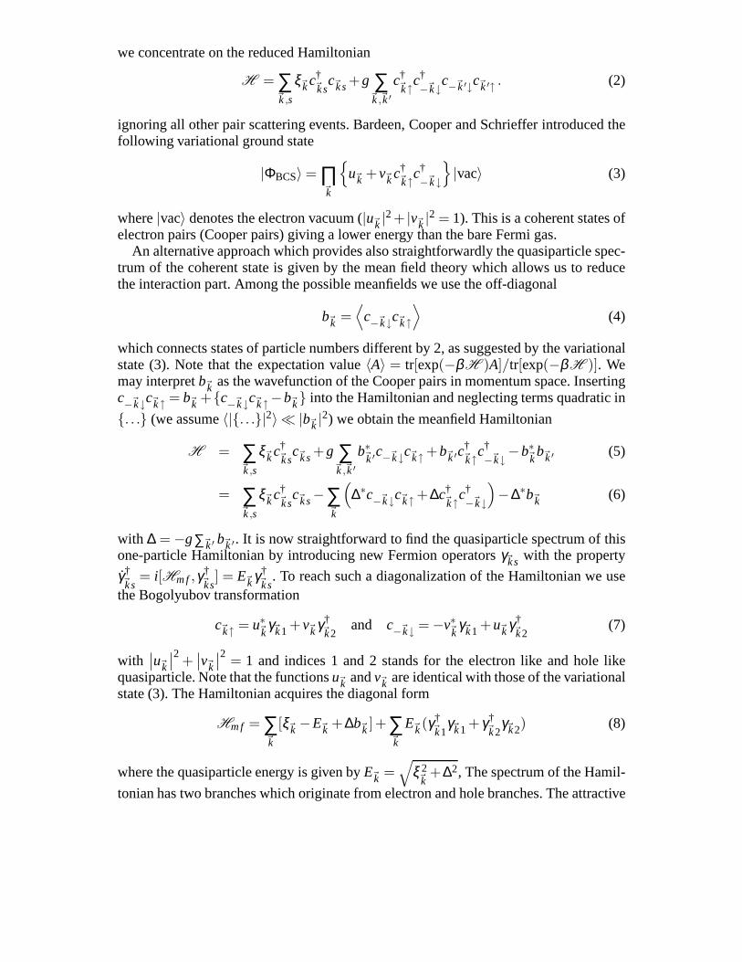
FIGURE 1. Schematic quasiparticle spectrum: The solid line shows thespectrum with a finite energygap and the dashed line corresponds to the spectrum for∆ = 0 with the same quasiparticle occupation.States withE < 0 are occupied by quasiparticles and empty forE > 0. Obviously the opening of the gaplowers the groundstate energy.

interactiong leads to an instability of the Fermi surface and the opening of a gap 2∆ (seeFig.1). The gap is the result of ’hybridizing’ electron-like and hole-like quasiparticlesleading to new quasiparticles as a superposition of electron- and hole-like character.

The energy gap has to be determined self-consistently from the ”gap equation”:

∆ = −g∑~k

b~k = −g∑~k

u∗~kv~k [1− f (E~k)] = −g∑~k

∆2E~k

tanh

(E~k

kBT

)(9)

with the Fermi factorf (E) = 1/(1+ eE/kBT). Note that this energy gap∆(T) onlydepends on temperature. We define the critical temperatureTc as the temperature wherethe gap vanishes. In the limit∆ → 0 of Eq.(9) we obtain the linearized gap equationdeterminingTc:

∆ = −g∆∑~k

12ξ~k

tanh

( ξ~k

kBT

)⇒ 1 = −g

∫dξ

N(ξ )

2ξtanh

(ξ

kBTc

). (10)

whereN(ξ ) is the density of states of the electrons. This integral has alogarithmicdivergence forξ →±∞. Thus we need to introduce a cutoff energyεc to obtain sensibleresult. This corresponds to a characteristic energy scale of the attactive interaction andis assumed to be much smaller than the Fermi energy or the bandwidth, the electronicenergy scale. In other words we may say that the attractive interaction is only presentin a narrow energy range around the Fermi surface. Then it seems legitimate to assumethat the density of states is constant,N(ξ ) → N0, yielding:

1 = −gN0

∫ εc

−εc

dξξ

tanh

(ξ

2kBTc

)= −gN0ln

(1.14εc

kBTc

)(11)

from which we derivekBTc = 1.14εce

−1/|g|N0 . (12)

The critical temperatureTc depends on the cutoff energyεc.The energy gap at zero temperature is also straightforwardly calculated using the same

energy cutoff:

1 = −gN0

∫ εc

0

dξ√ξ 2+∆2

= −gN0sinh−1 εc

∆(13)

such that∆(T = 0) ≈ 2εce−1/|g|N0 = 1.764kBTc . (14)

Obviously we can express the gap byTc with a universal proportionality factor andwithout the appearance ofεc. This is the signature of the scheme which we call ”weak-coupling” approximation. It is possible to express physical quantities cutoff-free, ifTc isknown.

Finally we estimate the condensation energy atT = 0 which corresponds to the energygain due to the opening of the gap. Since this gap is very smallthe condensation energyoriginates from the modification of the quasi particle states very close to the Fermienergy. Therefore we obtain

Econd= ∑~k

[ξ~k −E~k +∆b~k

]≈−1

2N0 |∆|2 . (15)

The condensation energy depends on the density of states at the Fermi surface and thezero-temperature gap magnitude. Thus within the weak coupling meanfield treatmentEcond is determined by the modified quasiparticle spectrum only (Fig.1).

Electron-Phonon interaction and Coulomb Repulsion

So far the nature of the model interaction was not specified inour discussion. We nowturn to the electron-phonon mediated interaction and whichclosely connected with theCoulomb interaction. Thus, it is necessary examine also theeffect of Coulomb repulsionon the pairing of electrons. Electron possesses charge and spin degrees of freedom. Ina metal Coulomb interaction coupling to charge is renormalized through many bodyeffects.

V~k,~k ′ =4πe2

q2ε(~q,ω)(16)

where~q = ~k −~k ′. The dielectric constantε(~q,ω) describes the effect of dynamicalscreening of charge fluctuations. This occurs due to the rearrangement of the electronsas well as the polarization of the elastic (positively charged) ionic lattice of the metal i.e.due to phonons. We can decompose the renormalized interaction into two correspondingparts

Veff~k,~k ′ =

4πe2

q2+k2T F︸ ︷︷ ︸

renorm. Coulomb

+4πe2

q2+k2T F

ω2q

ω2−ω2q︸ ︷︷ ︸

electron-phonon

, (17)

with hω = ε~k −ε~k ′. where the first is due Thomas-Fermi screening which is consideredas instantaneous so that we ignore the frequency dependence. The screening length is

λTF = k−1T F with k2

TF =6πe2ne

εF, (18)

which is of the order of a few lattice constants, making the interaction very shortranged. The second part due to the phonons, in the same way short ranged, involves thedynamics of the ions which slow compared electronic time scales. Hereωq describesthe spectrum of the acoustic phononsωq = sqat long wave-lengths, implying the DebyeenergyhωD as a characteristic energy scale. This interaction is attractive for frequencies|ω| < ωq ≤ ωD and repulsive otherwise. In this way the Debey frequency appears as anatural energy cutoffεc. We will now use a simple model given by Anderson and Morelto discuss the superconducting instability including the repulsive part of the Coulombinteraction which we had ignored in the introduction above [30].

Anderson-Morel-Model

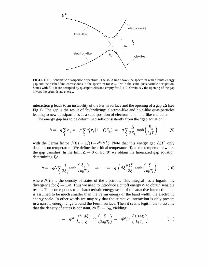
Including now also the effect of the repulsive Coulomb interaction we set up asimplified weak-coupling model which keeps the most essential features of the electronband and the structure of the interaction (17). The electronband is characterized by itswidthW = 2EF with the chemical potential in the center and a constant density of statesN(ξ ) = N0. The interaction is divided into a repulsive and an attractive partVeeandVep,respectively, originating from the two parts in (17). The energy range of the attractivepart is centered around the Fermi energy bounded by the cutoff energyεD = hωD whilethe repulsive part extends over the whole band width. Thus wedefine

V~k,~k ′ = Vee~k,~k′ +Vep

~k ,~k′

⇒

N0Vee~k,~k′ = N0Vee(ξ~k ,ξ~k ′) =

µ > 0 for−W ≤ ξ~k ,ξ~k ′ ≤W0 else

N0Vep~k,~k′ = N0Vep(ξ~k ,ξ~k ′) =

−λ < 0 for− εD ≤ ξ~k ,ξ~k ′ ≤ εD

0 else(19)

with ξ~k = ε~k − εF . We set up the corresponding BCS-type Hamiltonian with the mo-mentum dependent interaction

H = ∑~k,s

ξ~kc†~k ,s

c~k,s+1

2Ω ∑~k,~k ′

V~k,~k ′c†~k↑c

†−~k↓c−~k ′↓c~k ′↑ (20)

which we decouple in the analogous way as in the previous section leading to the gapequation

∆~k = −∑~k ′

V~k,~k ′〈c−~k ′↓c~k ′↑〉 , ∆∗~k

= −∑~k ′

V~k,~k′〈c†~k ′↑c

†−~k ′↓〉 . (21)

ξD +εD +ε

D−εD−W +W ξ−ε

V V

−W +W

µλ

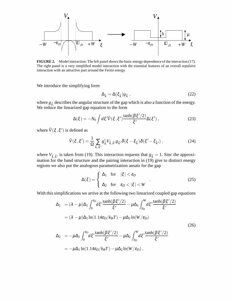
FIGURE 2. Model interaction: The left panel shows the basic energy dependence of the interaction (17).The right panel is a very simplified model interaction with the essential features of an overall repulsiveinteraction with an attractive part around the Fermi energy.

We introduce the simplifying form

∆~k = ∆(ξ~k)g~k , (22)

whereg~k describes the angular structure of the gap which is also a function of the energy.We reduce the linearized gap equation to the form

∆(ξ ) = −N0

∫dξ ′V(ξ ,ξ ′)

tanh(βξ ′/2)

ξ ′ ∆(ξ ′) , (23)

whereV(ξ ,ξ ′) is defined as

V(ξ ,ξ ′) =1Ω ∑

~k,~k′g∗~kV~k,~k′g~k ′δ (ξ −ξ~k)δ (ξ ′−ξ~k ′) . (24)

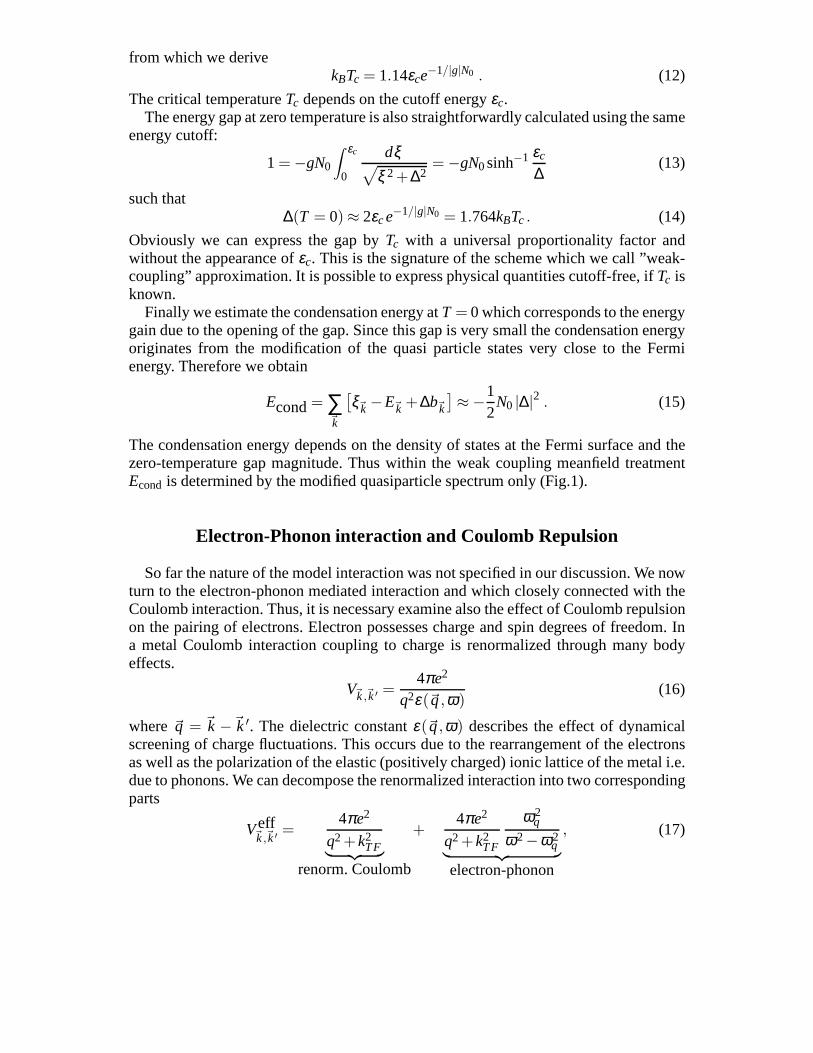
whereV~k,~k′ is taken from (19). This interaction requests thatg~k = 1. Sinc the approxi-mation for the band structure and the pairing interaction in(19) give to distinct energyregions we also put the analogous parametrization ansatz for the gap

∆(ξ ) =

∆1 for |ξ | < εD

∆2 for εD < |ξ | < W. (25)

With this simplifications we arrive at the following two linearized coupled gap equations

∆1 = (λ −µ)∆1

∫ εD

0dξ ′ tanh(βξ ′/2)

ξ ′ −µ∆2

∫ W

εD

dξ ′ tanh(βξ ′/2)

ξ ′

= (λ −µ)∆1 ln(1.14εD/kBT)−µ∆2 ln(W/εD)

∆2 = −µ∆1

∫ εD

0dξ ′ tanh(βξ ′/2)

ξ ′ −µ∆2

∫ W

εD

dξ ′ tanh(βξ ′/2)

ξ ′

= −µ∆1 ln(1.14εD/kBT)−µ∆2 ln(W/εD) .

(26)

ξ

N0 ∆1

∆2

−εD +εD

−W +W

−W +W

∆N( )

ξ

ξ

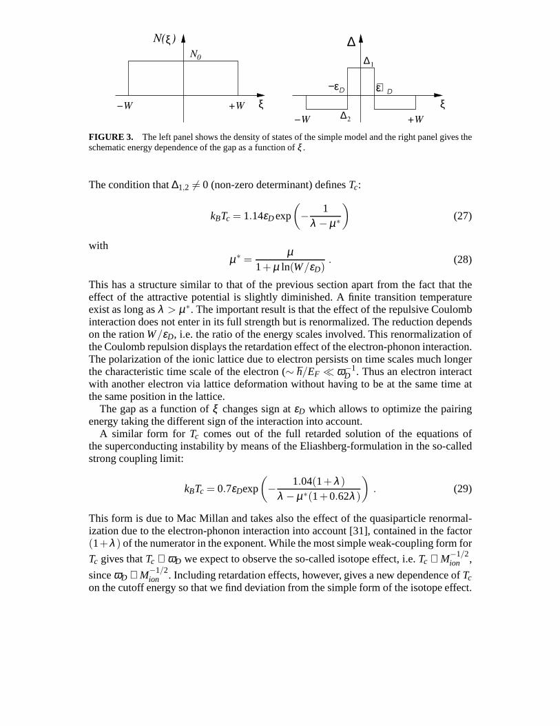
FIGURE 3. The left panel shows the density of states of the simple modeland the right panel gives theschematic energy dependence of the gap as a function ofξ .

The condition that∆1,2 6= 0 (non-zero determinant) definesTc:

kBTc = 1.14εD exp

(− 1

λ −µ∗

)(27)

withµ∗ =

µ1+ µ ln(W/εD)

. (28)

This has a structure similar to that of the previous section apart from the fact that theeffect of the attractive potential is slightly diminished.A finite transition temperatureexist as long asλ > µ∗. The important result is that the effect of the repulsive Coulombinteraction does not enter in its full strength but is renormalized. The reduction dependson the rationW/εD, i.e. the ratio of the energy scales involved. This renormalization ofthe Coulomb repulsion displays the retardation effect of the electron-phonon interaction.The polarization of the ionic lattice due to electron persists on time scales much longerthe characteristic time scale of the electron (∼ h/EF ω−1

D . Thus an electron interactwith another electron via lattice deformation without having to be at the same time atthe same position in the lattice.

The gap as a function ofξ changes sign atεD which allows to optimize the pairingenergy taking the different sign of the interaction into account.

A similar form for Tc comes out of the full retarded solution of the equations ofthe superconducting instability by means of the Eliashberg-formulation in the so-calledstrong coupling limit:

kBTc = 0.7εDexp

(− 1.04(1+λ )

λ −µ∗(1+0.62λ )

). (29)

This form is due to Mac Millan and takes also the effect of the quasiparticle renormal-ization due to the electron-phonon interaction into account [31], contained in the factor(1+λ ) of the numerator in the exponent. While the most simple weak-coupling form for

Tc gives thatTc ∝ ωD we expect to observe the so-called isotope effect, i.e.Tc ∝ M−1/2ion ,

sinceωD ∝ M−1/2ion . Including retardation effects, however, gives a new dependence ofTc

on the cutoff energy so that we find deviation from the simple form of the isotope effect.

Strongly correlated electron systems

In simple metals it is rather easy for the electron-phonon interaction to overcome theCoulomb repulsion through the retardation effect. The conduction electrons are muchfaster than the ions and move basically as free particles. Inso-called strongly correlatedelectron systems, however, electrons are often more close associated with atomic orbitalsand retain more of their localized character, like in transition metal oxides or rare-earthintermetallics forming so-called heavy Fermion systems. The nearly localized electronsare considerably slower in their motion such that Coulomb interactions are comparableto the kinetic energy or even larger. In the heavy Fermion materials the characteristicenergy scale associated with the carriers at the Fermi energy is even smaller that theDebye energy. Under such conditions the retardation effectdoes not provide sufficienthelp and Coulomb interaction dominates over the attractiveelectron-phonon coupling.

Symmetry of the pair wave function

Both the Coulomb and the electron-phonon interaction are very short ranged and maybe viewed practically as contact interactions so that they are felt by two electrons onlyif they can be found with a finite probability at the same spot.Considering the pairwavefunction

ψ(~r ,s;~r ′,s′) = f (∣∣~r −~r ′

∣∣)χ(s,s′) (30)

the obital partf (~r ) has to be in thel = 0-channel for a rotationally symmetric systemsand the spin configuration has spin-singlet character (onlyparticles of the opposite spincan meet at the same point). Forλ < µ∗ the Cooper pairing instability is suppressed byCoulomb interaction. The short-ranged repulsive interaction can be avoided by electronpairs with a non-vanishing orbital angular momentuml > 0. Then the pair wavefunc-tion vanishes for the two electrons at the same place (f (r) ∝ r l for r → 0). Cooper pairsin a rotationally symmetric environment satisfy the following basic symmetry require-ments. The fact that two identical Fermions pair requires that their wave functions isantisymmetric under exchange of the two electrons yields following conditions:

ψ(~r ′,s′;~r ,s) = −ψ(~r ,s;~r ′,s′) = f (−~r −~r ′)χs′,s

⇒

f (−~r ) = f (~r ), χs,s′ = −χs′,s, l = 0,2,4, ..., S= 0

f (−~r ) = − f (~r ), χs,s′ = χs′,s, l = 1,3,5, ..., S= 1

(31)

As parity is given by(−1)l , even partity means spin singlet and odd parity meansspin triplet pairing. From this viewpoint we define a conventional superconductor as acondensate ofl = 0 Cooper pairs, i.e. the most symmetric pairing state. Unconventionalare all other states withl > 0. This distinction is not restricted to rotation symmetricsystems, but can be applied in the modified form also to real metals which possess(lower) point group symmetry of the crystalline lattices. There the angular momentumis replaced by the irreducible representations of the pointgroup, as we will see later.

Alternative mechanisms

If the short-ranged Coulomb repulsion jams the electron-phonon interaction for pair-ing, alternative pairing interactions have to be found. Both interactions are of less im-portance, if pairing is realized in a channel different fromthe most symmetric one.

g~k;s,s′ = 〈c−~k,sc~ks′〉 with ∑~k

g~k;s,s′ = 0 (32)

which means that there is no pairing amplitude for electronson the same position.Mechanisms giving rise to this kind of pairing should provide a not too short-rangedinteraction.

Kohn and Luttinger asked in 1965 the question whether pairing would be possiblebased poorly on Coulomb interaction [32]. Their pairing mechanism is based on apart of the renormalized Coulomb interaction which we had ignored. Due to the sharpFermi edge in metals the renormalized Coulomb interaction possesses also a long-rangeoscillatory tail. These are the Friedel oscillations giving rise to a potential of the large-rform

V(r) =cos2kF r

r3 . (33)

which has obviously both attractive as well as repulsive parts. Pairing states of higherangular momentum would be able to take advantage of the attractive portion ofV(r).The resulting critical temperature obtained from this interaction is

Tc

TF' e−(2l)4

(34)

with l > 0. Although the relevant energy scale is the Fermi energy or band width, thismechanism is irrelevant for real superconductivity, sinceeven forl = 1 the achievableTcwould be of order of 10−7×TF . Nevertheless it is possible to undergo a superconduct-ing transition at very low temperature if no other instability has happened. An approachresulting in more feasible critical temperatures was givenby Berk and Schrieffer [33],who studied the exchange of spin fluctuations. In contrast tothe electron-phonon inter-action and the Kohn-Luttinger mechanism which are based on the electron charge only,the spin plays the key role in this case.

Mechanism based on spin-fluctuation exchange

The electron-phonon mechanism is based on the polarizability of the elastic ioniclattice in a metal. In a similar way also spins can form a polarizable medium andyield an effective interaction among electrons. These polarizable spins can be localizeddegrees of freedom or the spins of the conduction electrons themselves. Nearly magneticmaterials are most suitable for this type of interaction. Wewill illustrate this here on theexample of a nearly ferromagnetic metal, described by the Stoner model.

We consider an electron with spin~S at the position~r and timet. By means ofthe exchange interaction (exchange hole) the electron spinpolarizes the spin of the

surrounding electrons. In this way it acts like a local magnetic field of the form

~H (~r , t) = − IµBh

~S(~r , t) (35)

whereµB is the Bohr magneton andI = U/Ω is derived from the exchange interaction

Hex=∫

d3rd3r ′Uδ (~r −~r ′)ρ↑(~r )ρ↓(~r′) (36)

which appears here as a repulsive contact interaction of strengthU between electrons ofopposite spin (ρs(~r ) denotes the density of electrons of spins at~r , Ω is the volume).According to linear response theory, the electron spins will respond to the local field asdescribed by the dynamical spin susceptibility

~S(~r ′, t ′) = µB

∫d3r dt χ(~r ′−~r , t ′− t) ~H (~r , t) (37)

assumingχ(~r , t) to be isotropic in spin space. Again invoking the exchange interactionit is possible to derive an effective Zeeman energy for the spin density at(~r ′, t ′).

∆E = −µB

h~S(~r ′, t ′) · ~H (~r ′, t ′) =

Ih~S(~r ′, t ′) ·µB

∫d3r dt χ(~r ′−~r , t ′− t)~H (~r , t) (38)

which can be reformulated in terms of electron spin densities,

Hs f = − I2

h2

∫d3r d3r ′

∫dt dt′ χ(~r −~r ′; t − t ′) ~S(~r , t) · ~S(~r ′, t ′) . (39)

and can be rewritten in momentum space as

Hs f =− 1Ω

I2

4

∫dω ∑

~q,~k,~k ′Re(χ(~q,ω)) ∑

s1,s2,s3,s4

c†~k+~q,s1

~σ s1s2c~k,s2·c†

~k ′−~q,s3~σ s3s4c~k ′,s4

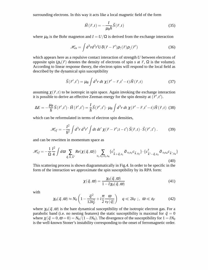
(40)This scattering process is shown diagrammatically in Fig.4. In order to be specific in theform of the interaction we approximate the spin susceptibility by its RPA form:

χ(~q,ω) =χ0(~q,ω)

1− I χ0(~q,ω)(41)

with

χ0(~q,ω) ≈ N0

(1− ~q2

12k2F

+ iπ2

ωvF |~q|

)q 2kF ; , ω εF (42)

whereχ0(~q,ω) is the bare dynamical susceptibility of the isotropic electron gas. For aparabolic band (i.e. no nesting features) the static susceptibility is maximal for ~q = 0whereχ(~q = 0,ω = 0) = N0/(1− IN0). The divergence of the susceptibility for 1= IN0is the well-known Stoner’s instability corresponding to the onset of ferromagnetic order.

Iχ ω

k

k+q

k’

k’−q

σ σI(q, )

FIGURE 4. Process of pair scattering of electrons due to spin flucutions, i.e. paramagnon exchange.

Re

(q,0

)χ

(q, )

ωχ

Im

q ω0q ω

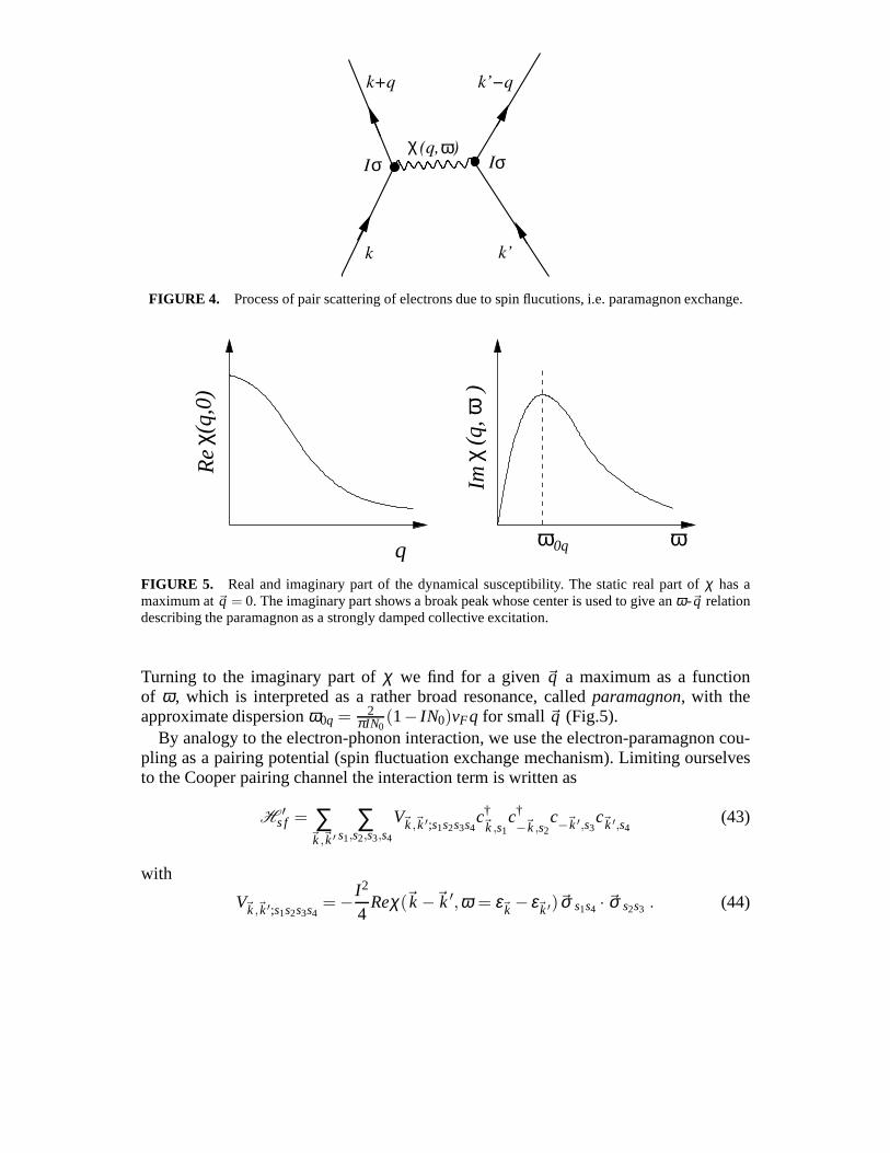
FIGURE 5. Real and imaginary part of the dynamical susceptibility. The static real part ofχ has amaximum at~q = 0. The imaginary part shows a broak peak whose center is used to give anω-~q relationdescribing the paramagnon as a strongly damped collective excitation.

Turning to the imaginary part ofχ we find for a given~q a maximum as a functionof ω, which is interpreted as a rather broad resonance, calledparamagnon, with theapproximate dispersionω0q = 2

πIN0(1− IN0)vFq for small~q (Fig.5).

By analogy to the electron-phonon interaction, we use the electron-paramagnon cou-pling as a pairing potential (spin fluctuation exchange mechanism). Limiting ourselvesto the Cooper pairing channel the interaction term is written as

H′

s f = ∑~k,~k ′

∑s1,s2,s3,s4

V~k,~k ′;s1s2s3s4c†~k ,s1

c†−~k,s2

c−~k ′,s3c~k ′,s4

(43)

with

V~k,~k′;s1s2s3s4= − I2

4Reχ(~k −~k ′,ω = ε~k − ε~k ′)~σ s1s4 · ~σ s2s3 . (44)

Since the Cooper scattering matrix element is spin dependent, we obtain different valuesfor the spin-singlet and spin-triplet configuration:

Vs~k,~k ′ =

3I2

4Reχ(~k −~k ′,ω = ε~k − ε~k ′) for S= 0 ,

Vt~k,~k ′ = − I2

4Reχ(~k −~k ′,ω = ε~k − ε~k ′) for S= 1 ,

(45)

Obviously this is repulsive for the singlet, but attractivein the triplet channel. Thusodd-parity pairing states are favored withl = 1,3,5, .... Similar to electron-phononinteraction retardation effects play a role. The attraction is obtained roughly within anenergy rangeω < ω0q providing the natural energy cutoff from the maximal paramagnonresonance energy forq∼ 2kF :

εc =8

π IN0(1− IN0)EF (46)

It is important to notice thatεc EF near the Stoner instability, an effect of the so-calledcritical slowing down (spin fluctuations become slower). Examining all possibilities wefind that thel = 1-state is the most favored odd-parity state of this interaction. We choosefor the gap function∆~k = ∆g~k with

gα~k

= Ylα(k) =

1√2k

(kx + iky) α = +1

kz

kα = 0

1√2k

(kx− iky) α = −1

, (47)

the threel = 1 spherical harmonics (k =~k/k). Projecting with thisg~k we define

V(ξ ,ξ ′) = − I2

4Ω ∑~k,~k ′

gα~k

χ(~k −~k ′,ω = 0)gα~k′δ (ξ −ξ~k)δ (ξ ′−ξ~k ′)

≈

V1 |ξ |, |ξ ′| < εc

0 otherwise

(48)

where

V1 = − I12

IN0

(1− IN0)2 . (49)

Since we are now left with a BCS-like formulation, it is straightforward to derive thecritical temperature is

kBTc = εce−1/λs , (50)

with

λs = N0V1 =112

(IN0

1− IN0

)2

. (51)

Assuming the Coulomb repulsion as a contact interaction we do not have a correction inthe exponent in the case ofl > 0. It is important note here that while the Coulomb andelectron-phonon interaction has usually the range of the Thomas-Fermi screening length,the paramagnon mediated interaction is longer ranged with the magnetic correlationlengthξ as the length scale. The correlation length is defined as

ξ 2s ∼

∫d3rr 2〈~S(~r ) · ~S(0)〉 (52)

Since we have an Ornstein-Zernike form for the static susceptibility, we can write forthe static susceptibility

χ(~q) ∝1

1+ξ 2s ~q2 (53)

which compared with (42, 41) leads to

ξ 2s =

1

12k2F

IN0

1− IN0. (54)

The correlation length diverges at the Stoner instability point favoring higher angularmomentum pairing. Eventually the~q-dependence of the pairing interaction apart fromthe spin dependence, is decisive for the choice of the pairing state.

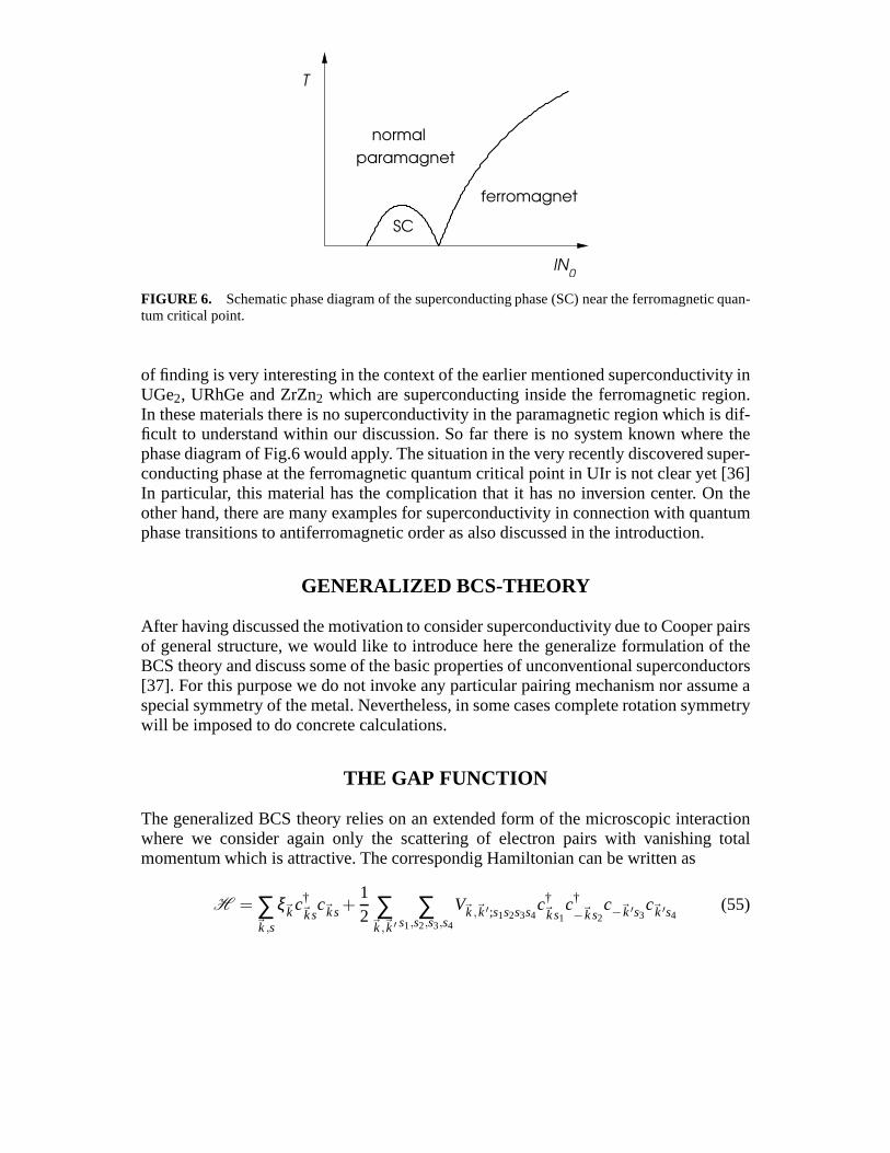
Superconducitivity in the vicinity of magnetic quantum cri tical point

Based on these considerations we construct now a phase diagram for the spin tripletstate near a quantum phase transition to ferromagnetic order. Although we have donesome rough approximations, a qualitative view is still illustrative. The Stoner-criterion1− IN0 = 0 defines the zero-temperature transition point so that we may takeIN0 as thecontrolling parameter which might be changed in real material, for example, by applyingpressure. ForIN0 > 1 the metal has a finite Curie-temperatureTC ∝ (IN0−1)1/2 ( in thestandard mean field approach).

In the paramagnetic region there are two basic trends determining the superconductingtransition temperatureTc. The coupling constantV1 diverges while the cutoff energyεcvanishes at the quantum critical point. This gives rise to the non-monotonous behaviorof Tc which passes a maximum with increasingIN0 and vanishing at the quantum criticalpoint. While the exact behavior is modified by the renormalization of the quasiparticleweight close to the quantum critical point which has been ignored here, the fact thatTcgoes through a maximum and disappears right at the quantum critical point. [34, 35].

We do not touch here the question whether superconductivitywould also appear in-side the ferromagnetic phase within our theory. It has been shown by Fay and Appel thatspin polarized pairing states (so-called non-unitary states) are possible [34]. This kind

normal

T

IN0

SC

ferromagnet

paramagnet

FIGURE 6. Schematic phase diagram of the superconducting phase (SC) near the ferromagnetic quan-tum critical point.

of finding is very interesting in the context of the earlier mentioned superconductivity inUGe2, URhGe and ZrZn2 which are superconducting inside the ferromagnetic region.In these materials there is no superconductivity in the paramagnetic region which is dif-ficult to understand within our discussion. So far there is nosystem known where thephase diagram of Fig.6 would apply. The situation in the veryrecently discovered super-conducting phase at the ferromagnetic quantum critical point in UIr is not clear yet [36]In particular, this material has the complication that it has no inversion center. On theother hand, there are many examples for superconductivity in connection with quantumphase transitions to antiferromagnetic order as also discussed in the introduction.

GENERALIZED BCS-THEORY

After having discussed the motivation to consider superconductivity due to Cooper pairsof general structure, we would like to introduce here the generalize formulation of theBCS theory and discuss some of the basic properties of unconventional superconductors[37]. For this purpose we do not invoke any particular pairing mechanism nor assume aspecial symmetry of the metal. Nevertheless, in some cases complete rotation symmetrywill be imposed to do concrete calculations.

THE GAP FUNCTION

The generalized BCS theory relies on an extended form of the microscopic interactionwhere we consider again only the scattering of electron pairs with vanishing totalmomentum which is attractive. The correspondig Hamiltonian can be written as

H = ∑~k,s

ξ~kc†~ks

c~ks+12 ∑

~k,~k ′∑

s1,s2,s3,s4

V~k,~k′;s1s2s3s4c†~ks1

c†−~k s2

c−~k ′s3c~k ′s4

(55)

with pair scattering matrix elements

V~k,~k ′;s1s2s3s4= 〈−~k,s1;~k,s2|V|−~k ′,s3;~k ′,s4〉 . (56)

Due to Fermionic anticommutation rules the following relations must hold

V~k,~k ′;s1s2s3s4= −V−~k,~k ′;s2s1s3s4

= −V~k,−~k ′;s1s2s4s3= V−~k,−~k ′;s2s1s4s3

. (57)

We consider a weak-coupling approach with an interaction attractive in an energy rangedefined by a cutoffεc, i.e. the scattering matrix elements are non-zero for−εc <ξ~k ,ξ~k ′ < εc εc andεc EF .

Analogous to the simple case we introduce an off-diagonal mean-field

b~k,ss′ = 〈c−~ksc~ks′〉 (58)

which leads to the mean field Hamiltonian

H′ = ∑

~k,s

ξ~kc†~ks

c~ks−12 ∑

~k,s1,s2

[∆~k,s1s2

c†~k s1

c†−~k s2

+∆∗~k,s1s2

c~k s1c−~ks2

]+K +small terms,

(59)where

K = −12 ∑

~k,~k ′∑

s1,s2,s3,s4

V~k,~k ′;s1s2s3s4〈c†

~ks1c†−~ks2

〉〈c−~k ′s3c~k ′s4

〉. (60)

The generalized gap∆~k;ss′ are defined as a function of~k and the spins(s,s′) by theself-consistent equations

∆~k,ss′ = − ∑~k ′,s3s4

V~k,~k′;ss′s3s4b~k,s3s4

,

∆∗~k,ss′

= − ∑~k ′s1s2

V~k ′,~k;s1s2s′sb∗~k,s2s3

.(61)

The gap function is now a complex 2×2 complex matrix in spin space

∆~k =

( ∆~k,↑↑ ∆~k,↑↓∆~k,↓↑ ∆~k,↓↓

). (62)

The structure of the gap function is related to the wave function of the Cooper pairs,b~k,s1s2

. In order to get a deeper insight into the symmetry properties of the gap function,we separateb~k,s1,s2

into an orbital part and a spin part

b~k,s1s2= φ(~k)χs1s2 , (63)

The parity of the orbital part and the spin configuration are linked due to the antisym-metry condition of the many-Fermion wave functions as mentioned above:

Even Parity: φ(~k) = φ(−~k) ⇔ χs1s2 = 1√2(| ↑↓〉− | ↓↑〉) spin singlet

Odd Parity: φ(~k) = −φ(−~k) ⇔ χs1s2 =

| ↑↑〉

1√2

(| ↑↓〉+ | ↓↑〉)

| ↓↓〉

spin triplet

(64)Consequently, the gap function obeys the following rules:

∆~k,s1s2= −∆−~k,s2s1

=

∆−~k,s1s2= −∆~k ,s2s1

even

−∆−~k ,s1s2= ∆~k,s2s1

odd(65)

or in short notation∆~k = −∆T

−~k(66)

Based on these points, we parametrize the form of the 2×2 matrix representing the gapfunction. For even parity (spin singlet), we only need a scalar functionψ(~k),

∆~k =

( ∆~k,↑↑ ∆~k,↑↓∆~k,↓↑ ∆~k,↓↓

)=

(0 ψ(~k)

−ψ(~k) 0

)= iσyψ(~k) . (67)

which satisfiesψ(~k) = ψ(−~k). For the odd parity case, the spin triplet configurationhas to be represented by three components which we introducte as the vector function~d(~k) in the following form

∆~k =

( ∆~k,↑↑ ∆~k,↑↓∆~k,↓↑ ∆~k,↓↓

)=

(−dx(~k)+ idy(~k) dz(~k)

dz(~k) dx(~k)+ idy(~k)

)= i(

~d(~k) · ~σ)

σy ,

(68)with ~d(~k) = − ~d(−~k). This notation will turn out to be very useful considering rota-tions in spin space as will see shortly. We find that

∆~k ∆†~k

= |ψ(~k)|2σ0 spin singlet

∆~k ∆†~k

= | ~d |2σ0+ i( ~d × ~d∗) · ~σ spin triplet.(69)

While for the spin singlet case leads always to∆~k ∆†~k

∝ σ0, the unit matrix, in the spintriplet channel also components different fromσ0 is possible. Pairing states with non-zero~q(~k) = i ~d(~k)× ~d(~k)∗ are callednon-unitaryand are related to pairing with someintrinsic spin polarization, since~q(~k) is connected with the spin expectation value

tr[∆~k ∆†~k

~σ ] for momentum~k. As will become clear below a necessary condition for~q 6= 0 is broken time reversal symmetry.

Symmetry aspects

Cooper pairs consist of two electrons of opposite momentum (⇒ zero-momentumpairs) which are degenerate in energy. There are certain keysymmetries which guaranteethe possibility to find such states at the Fermi energy.

For spin singlet pairing the key symmetry is time reversal invariance [38]. Startingwith an electronic state with momentum~k and spin up↑, we obtain a proper degeneratepartner state by time reversalK:

K|~k ↑〉 = |−~k,↓〉 (70)

such that we have the necessary partner states to form spin singlet Cooper pairs:|~k ↑〉, |−~k ↓〉.

Spin triplet pairing requires in addtion to time reversal the inversion symmetryI togenerate the proper partner states [39]. We start from the same state and obtain

K|~k ↑〉 = |−~k,↓〉 , I |~k ↑〉 = |−~k,↑〉 , I K|~k ↑〉 = |~k,↓〉 (71)

which allows us to form all possible spin triplet configurations.

We want to review the important symmetries and examine theireffect on the gapfunctions. This will be important in the future discussion of the superconducting phases,in particular, in the context of phenomenological description. The symmetries relevantto us are rotations in real and spin space, time reversal, inversion andU(1)-gaugesymmetry.Orbital rotation:

gc~k,s = cR(g)~k,s gc†~k,s

= c†R(g)~k,s

(72)

g∆~k = ∆R(g)~k (73)

whereR(g) is the rotation matrix in three dimensiona corresponding the operation ofg.Spin rotation:

gc~ks = ∑s′

DS (g)ss′c~ks′ and gc†~ks

= ∑s′

DS (g)∗s′sc†~ks′

(74)

g∆~k = DτS

(g)∆~kDS (g). (75)

whereDS (g) = ei~S·~φ (76)

with ~φ the rotation vector of the operationg. Spin rotation has naturally no influence ona singlet configuration because the total spin is zero. On theother hand, the triplet case

corresponds to the usual rotation applied on the~d -vector

g~d(~k) = RS (g) ~d(~k) (77)

with RS (g) the three-dimensional representation of the corresponding rotation. Onewould note that the gap function is then represented in spin space as a spin pointingalong the~d -vector

dx−| ↑↑〉+ | ↓↓〉− idy| ↑↑〉+ | ↓↓〉+dz| ↑↓〉+ | ↓↑〉 (78)

This rather simple behavior under spin rotation is the benefit of the above parametriza-tion of the gap function.Time-reversal symmetryK

Kc~ks= ∑s′

(−iσy)ss′c†−~k,s′

(79)

K∆~k = σy∆∗~k

σy (80)

We usedK = −iσyC with C the operator of complex-conjugation. Note thatK isantilinear.Inversion symmetryI

Ic~k ,s = c−~k ,s ⇒ I ∆~k = ∆−~k =

+∆~k spin-singlet

−∆~k spin-triplet(81)

U(1)-gauge symmetry:

Φc~ks = eiφ/2 ⇒ Φ∆~k = ∆~keiφ (82)

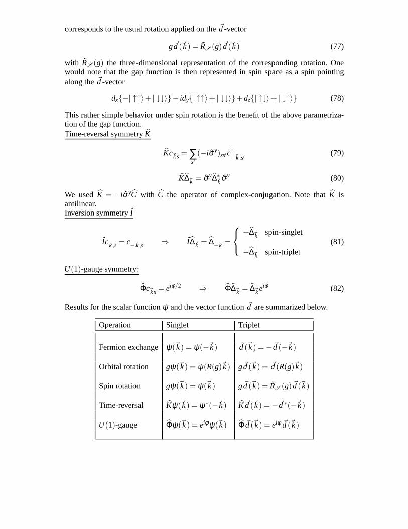
Results for the scalar functionψ and the vector function~d are summarized below.

Operation Singlet Triplet

Fermion exchange ψ(~k) = ψ(−~k) ~d(~k) = − ~d(−~k)

Orbital rotation gψ(~k) = ψ(R(g)~k) g~d(~k) = ~d(R(g)~k)

Spin rotation gψ(~k) = ψ(~k) g~d(~k) = RS (g) ~d(~k)

Time-reversal Kψ(~k) = ψ∗(−~k) K ~d(~k) = − ~d ∗(−~k)

U(1)-gauge Φψ(~k) = eiφ ψ(~k) Φ ~d(~k) = eiφ ~d(~k)

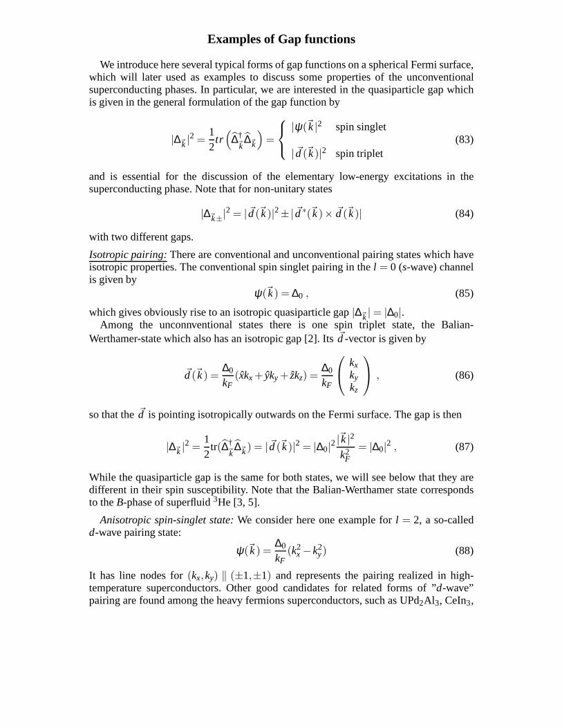
Examples of Gap functions

We introduce here several typical forms of gap functions on aspherical Fermi surface,which will later used as examples to discuss some propertiesof the unconventionalsuperconducting phases. In particular, we are interested in the quasiparticle gap whichis given in the general formulation of the gap function by

|∆~k |2 =

12

tr(

Ơ~k

∆~k

)=

|ψ(~k|2 spin singlet

| ~d(~k)|2 spin triplet(83)

and is essential for the discussion of the elementary low-energy excitations in thesuperconducting phase. Note that for non-unitary states

|∆~k±|2 = | ~d(~k)|2±| ~d∗(~k)× ~d(~k)| (84)

with two different gaps.

Isotropic pairing:There are conventional and unconventional pairing states which haveisotropic properties. The conventional spin singlet pairing in thel = 0 (s-wave) channelis given by

ψ(~k) = ∆0 , (85)

which gives obviously rise to an isotropic quasiparticle gap |∆~k | = |∆0|.Among the unconnventional states there is one spin triplet state, the Balian-

Werthamer-state which also has an isotropic gap [2]. Its~d -vector is given by

~d(~k) =∆0

kF(xkx + yky + zkz) =

∆0

kF

kxkykz

, (86)

so that the~d is pointing isotropically outwards on the Fermi surface. The gap is then

|∆~k |2 =

12

tr(Ơ~k

∆~k) = | ~d(~k)|2 = |∆0|2|~k|2k2

F

= |∆0|2 , (87)

While the quasiparticle gap is the same for both states, we will see below that they aredifferent in their spin susceptibility. Note that the Balian-Werthamer state correspondsto theB-phase of superfluid3He [3, 5].

Anisotropic spin-singlet state:We consider here one example forl = 2, a so-calledd-wave pairing state:

ψ(~k) =∆0

kF(k2

x −k2y) (88)

It has line nodes for(kx,ky) ‖ (±1,±1) and represents the pairing realized in high-temperature superconductors. Other good candidates for related forms of ”d-wave”pairing are found among the heavy fermions superconductors, such as UPd2Al3, CeIn3,

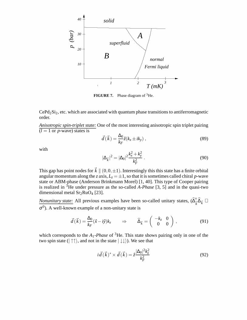
superfluid

30

10

20

40

p (b

ar)

B

A

1 2 3T (mK)

solid

Fermi liquid

normal

FIGURE 7. Phase diagram of3He.

CePd2Si2, etc. which are associated with quantum phase transitions to antiferromagneticorder.

Anisotropic spin-triplet state:One of the most interesting anisotropic spin triplet pairing(l = 1 or p-wave) states is

~d(~k) =∆0

kFz(kx± iky) , (89)

with

|∆~k |2 = |∆0|2

k2x +k2

y

k2F

. (90)

This gap has point nodes for~k ‖ (0,0,±1). Interestingly this this state has a finite orbitalangular momentum along thezaxis,Lz =±1, so that it is sometimes called chiralp-wavestate or ABM-phase (Anderson Brinkmann Morel) [1, 40]. Thistype of Cooper pairingis realized in3He under pressure as the so-calledA-Phase[3, 5] and in the quasi-twodimensional metal Sr2RuO4 [23].

Nonunitary state:All previous examples have been so-called unitary states, (Ơ~k

∆~k ∝σ0). A well-known example of a non-unitary state is

~d(~k) =∆0

kF(x− iy)kz ⇒ ∆~k =

(−kz 00 0

), (91)

which corresponds to theA1-Phaseof 3He. This state shows pairing only in one of thetwo spin state (| ↑↑〉, and not in the state| ↓↓〉). We see that

i ~d(~k)∗× ~d(~k) = z|∆0|2k2

z

k2F

(92)

gives the spin expectation value for the Cooper pair. This state leaves half of all electronsunpaired and is hard to stabilize due to reduced condensation energy. In3He it appearsonly in magnetic field which provides a bias for different spin directions. A similarbias appears of course also in ferromagnetic metals. Thus the superconducting phases inUGe2, URhGe and ZnZr2 are most likely non-unitary.

Bogolyubov Quasiparticles and Self-Consistent Equations

We can diagonalize the mean-field Hamiltonian (59) by means of Bogolyubov trans-formation. It is convenient to rewrite (59) in the followingform

H = ∑~k

C†~kE~kC~k +K , (93)

with

C~k =

c~k↑c~k↓

c†−~k↑

c†−~k↓

and E~k =

12

ξ~k σ0 ∆~k

Ơ~k

−ξ~k σ0

. (94)

We are now searching the diagonalized form

H = ∑~k

A†~k

E~kA~k +K (95)

where

A~k =

a~k↑a~k↓

a†−~k↑

a†−~k↓

and E~k =

E~k+0 0 0

0 E~k− 0 00 0 −E−~k+

00 0 0 −E~k−

. (96)

The Bogolyubov transformation is given by the unitary matrix U~k with

U~k =

u~k v~k

v∗−~ku∗−~k

⇒ C~k = U~kA~k and E~k = U†~kE~kU~k (97)

andU~kU†~k

= U†~k

U~k = 1.We restrict ourselves to the case of unitary pairing. This ensures thatE~k = E~k+

=E~k−. The solution of the eigenvalue problem leads tou~k andv~k

u~k =(E~k +ξ~k)σ0√2E~k(E~k +ξ~k)

and v~k =−∆~k√

2E~k(E~k +ξ~k)(98)

and the energy

E~k =√

ξ 2~k

+ |∆~k |2 with |∆~k |2 =

12

tr(

Ơ~k

∆~k

). (99)

With the new quasiparticle operators (61) we can express theself-consistence or gapequation using〈a†

~ksa~k ′s′〉 = δ~k~k ′δss′ f (E~k) where f (E) = 1/(exp(E/kBT) + 1) is the

Fermi distribution function:

∆~k,s1s2= − ∑

~k ′,s3s4

V~k,~k ′;s1s2s3s4

∑s′

v~k s4s′u~ks′s3〈a−~ks′a

†~ks′

〉−u~ks4s′v~ks′s3〈a†

~ks′a~ks′〉

= − ∑~k ′,s3s4

V~k,~k ′;s1s2s3s4

∆~k ′,s4s3

2E~k

tanh

(E~k

2kBT

)

(100)We introduce now a newly parametrized pairing interaction term in order to obtain a

simpler form of the self-consistence equation,

V~k,~k ′;s1s2s3s4= J0

~k,~k ′σ0s1s4

σ0s2s3

+J~k,~k′ ~σ s1s4 · ~σ s2s3 , (101)

consisting of a spin independent or density-density term and spin-spin exchange cou-pling. In the following we assume that these interactions are only non-zero in a certainrange around the Fermi energy with a cutoff energyεc. For spin singlet pairing the gapequation can be expressed forψ(~k),

ψ(~k) = −∑~k ′

(J0~k,~k ′ −3J~k,~k ′)︸ ︷︷ ︸

= vs~k,~k ′

ψ(~k ′)2E~k ′

tanh

(E~k ′

2kBT

)(102)

and|∆~k |2 = |ψ(~k)|2. For spin triplet channel, the gap equation takes the form

~d(~k) = −∑~k ′

(J0~k,~k ′ +J~k,~k ′)︸ ︷︷ ︸

= vt~k,~k ′

~d(~k ′)2E~k ′

tanh

(E~k ′

2kBT

)(103)

with |∆~k |2 = | ~d(~k)|2.

Critical tempeature and gap magnitude atT = 0

The linearized gap equation can now be used to determine the critical temperature.We consider first the spin singlet case

ψ(~k) = −∑~k ′

vs~k,~k ′

ψ(~k ′)2ξ~k ′

tanh

( ξ~k ′

2kBT

)

= −N0〈vs~k,~k ′ψ(~k ′)〉~k′ ,FS

∫ εc

0dξ

1ξ

tanh

(ξ

2kBT

)

︸ ︷︷ ︸= ln(1.13εc/kBT)

(104)

where〈. . .〉~k,FS denotes the angular average over the Fermi surface. This equation canbe expressed as a eigenvalue problem

−λψ(~k) = −N0〈vs~k,~k ′ψ(~k ′)〉~k′ ,FS , (105)

leading tokBTc = 1.14εce

−1/λ . (106)

Hereλ is a dimensionless and positive parameter. The superconducting instability corre-sponds to the highest eigenvalue (highestTc) of (105) which determines also the structureof the Cooper pairs.

The spin-triplet case has an analogous gap equation which for the evaluation ofTctakes the form

−λ ~d(~k) = −N0〈vt~k,~k ′

~d(~k ′)〉~k ′,FS (107)

and the same type of solutions. Naturally the solution of theinstability problem isspecific to the pairing interaction.

We now turn to the zero-temperature limit and determine the gap for the case ofspin singlet pairing. We introduce∆m as the maximal gap and writeψ(~k) = ∆mg~k with|g~k | ≤ 1. The gap atT = 0 is obtained from the equation

∆mg~k = −N0

⟨

vs~k,~k ′∆mg~k ′

∫ εc

0dξ

1√ξ 2+ |∆mg~k ′|2

⟩

~k ′,FS

. (108)

Multiplying both sides with ˜g∗~k and averaging~k over the Fermi surface, using (105) andintegrating overξ , we obtain eventually

1 = −λ⟨|g~k |

2 ln

(2εc

|∆mg~k |

)⟩

~k ′,FS

= −λ ln

(2εc

∆m

)1−〈|g~k′ |2 ln(|g~k ′|)〉~k′,FS

.

(109)

From this we get the ratio of the maximal gap andTc to be

∆m

kBTc= 1.76 exp

(−〈|g~k ′|2 ln(|g~k′|)〉~k′,FS

)≥ 1.76 , (110)

While this ratio is universal for the isotropic Fermi surface in the case ˜g~k = 1, we seethat it in general depends on the gap anisotropy. Like in conventional superconductors,in this ratio the cutoff energy has been eliminated, such that we can express the gapmagnitude byTc, i.e. we are dealing with the weak-coupling limit.

Condensation energy atT = 0

We now compute the condensation energy atT = 0 within the weak coupling ap-proach. Starting from Hamiltonian (59), we obtain in the Bogolyubov transformed for-mulation

H′ =

12∑

~k,s

E~k

(a†~k,s

a~k,s−a−~k,sa†−~k,s

)+K . (111)

with

K =12 ∑

~k,s1,s2

∆∗~k,s1s2

∆~k,s2s1

2E~k

tanh

(E~k

2kBT

). (112)

Then, the condensation energy atT = 0 is given by

Econd = 〈H ′〉∆ −〈H ′〉∆=0 =12∑

~k,s

(ξ~k −E~k)+12 ∑

~k,s1,s2

∆∗~k,s1s2

∆~k,s2s1

2E~k

= 2N0

∫ εc

0dξ (ξ −〈

√ξ 2+ |∆~k |2〉~k,FS)+

⟨|∆~k |

2∫ εc

0dξ

1√ξ 2+ |∆~k |2

⟩

~k,FS

≈−N0

2〈|∆~k |

2〉~k,FS = −N0

2|∆m|2〈|g~k |

2〉~k,FS ,

(113)under the assumptions that|∆~k | εc and for simplicity, that N0 is isotropic.(For an anisotropic Fermi densityN0(k), we can extend this expressionEcond =−(1/2)〈N0(k)|∆~k |2〉~k,FS.) Using now (110) we can compare different condensationenergies

Econd = −N0

2〈|∆mg~k |

2〉~k,FS = −12

N0 (1.76kBTc)2〈|g~k |

2〉~k,FS exp(−〈|g~k |2 ln |g~k |〉~k,FS)

(114)It is now obvious that an isotropic gap under these conditions gives the largest gainin condensation energy and explains why among the spin triplet state the BW-state ismost stable, if no bias in the pairing interaction (spin-orbit coupling and strong couplingeffects) favors a different state.

Specific heat discontinuity at Tc

A characteristic feature of the second order normal-superconductor phase transitionis the jump in specific heat atTc which is related to the release of entropy through theopening of the gap at the Fermi surface. First, we write the specific heat starting fromthe general form for the entropy:

S= −2kB

Ω ∑~k

f (E~k)ln( f (E~k))+(1− f (E~k)) ln(1− f (E~k))

⇒

C = TdSdT

= − 2Ω ∑

~k

E~k

d f(E~k)

dT= −2N0

T

∫ +∞

−∞dξ⟨∂ f (E~k)

∂E~k

E2

~k− T

2∂ |∆m(T)|2

∂T|g~k |

2⟩

~k,FS(115)

The specific heat of the normal state is easily obtained by setting ∆m = 0,

Cn = −2N0

T

∫ +∞

−∞dξ

∂ f (ξ )

∂ξξ 2 ≈ 2π2k2

B

3N0T , (116)

with the standard Sommerfeld T-linear dependence. The jumpin specific heat dependson the variation of the gap with temperature. It can be expressed as

∆CCn

∣∣∣∣T=Tc

=C−Cn

Cn

∣∣∣∣T=Tc

=3

2π2k2BT

〈|g~k |2〉~k,FS

∂ |∆m(T)|2∂T

∣∣∣∣T→Tc−

= 1.43〈|g~k|2〉2

~k,FS

〈|g~k|4〉~k,FS(117)

This result infers that the specific heat discontinuity is less pronounced in anisotropicgap functions than in the isotropic case. The entropy changeis smaller for a given gapsize∆m in the anisotropic case, since quasiparticle excitations with lower energy are stillallowed.

To show the last equality in (117), the temperature dependence of ∆m has to bedetermined. For this purpose we return to the gap equation which we want to considernearTc. Using the definition ofλ we have the relation

1λ

= − ln

(TTc

)−∫ εc

0dξ

1ξ

tanh

(ξ

2kBT

). (118)

With this expression ofλ for an arbitraryT, we find

〈|g~k |2〉~k,FSln

(TTc

)=∫ εc

0dξ⟨|g~k |

2 1E~k

tanh

(E~k

2kBT

)⟩

~k,FS

−〈|g~k |2〉~k,FS

∫ εc

0dξ

1ξ

tanh

(ξ

2kBT

)

= |∆m|2b〈|g~k |4〉~k,FS

(119)

with

b = −∫ +∞

−∞dξ

ddξ 2

tanh(ξ/2kBTc)

2ξ

=

7ζ (3)

8π2k2BT2

c. (120)

Note thatζ (3) = ∑∞n=1n−3 ≈ 1.2 is theζ Riemann function. Thus, in the vicinity ofTc,

we have

|∆m(T)|2 ≈〈|g~k |2〉~k,FS

b〈|g~k |4〉~k,FS

(1− T

Tc

)= 9.4 (kBTc)

2〈|g~k |2〉~k,FS

〈|g~k |4〉~k,FS

(1− T

Tc

)

= 5.3 |∆m(0)|2(

1− TTc

) 〈|g~k |2〉~k,FS

〈|g~k |4〉~k,FS

exp(〈|g~k |2 ln |g~k |〉~k,FS)

(121)

which inserted into (117) gives the result presented for thespecific heat discontinuity.This behavior of∆m(T) is general for the mean-field description of a second-order phasetransition.

Low Temperature Properties

The low temperature properties of superconductors are governed by the low-energyquasiparticle excitations. Thus, in the frame of generalized BCS theory, the key quantitywhich controls the thermodynamics is the quasiparticles density of states. As will be-come clear immediately, the topology of the nodes in the gap function is very decisivein this respect.

The density of states is defined as

N(E) =2Ω ∑

~k

δ (E~k −E) . (122)

where we use the Bogolyubov quasiparticles spectrum

E~k =√

ξ 2~k

+ |∆~k |2 . (123)

We decompose the~k-integral into the (radial) energyξ part and the angular part (averageover the Fermi surface):

N(E) = N0

∫ dΩ~k

4π

∫dξ δ (

√ξ 2+ |∆mg~k |2−E)

= N0

∫ dΩ~k

4πE√

E2−|∆mg~k |2= N0〈

E√E2−|∆mg~k |2

〉~k,FS .

(124)

line nodes

0

∆m ∆m ∆m

isotropicgapN(E)

EEE

point nodes

N

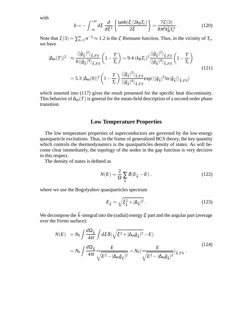
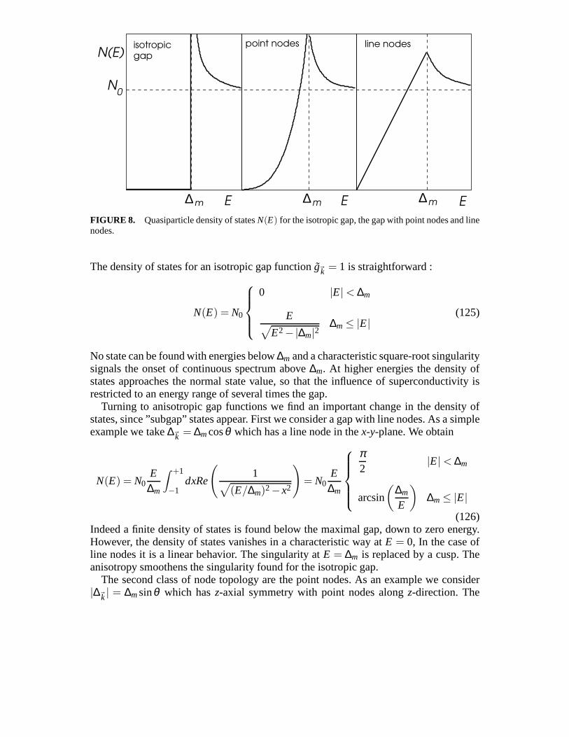
FIGURE 8. Quasiparticle density of statesN(E) for the isotropic gap, the gap with point nodes and linenodes.

The density of states for an isotropic gap function ˜g~k = 1 is straightforward :

N(E) = N0

0 |E| < ∆m

E√E2−|∆m|2

∆m ≤ |E|(125)

No state can be found with energies below∆m and a characteristic square-root singularitysignals the onset of continuous spectrum above∆m. At higher energies the density ofstates approaches the normal state value, so that the influence of superconductivity isrestricted to an energy range of several times the gap.

Turning to anisotropic gap functions we find an important change in the density ofstates, since ”subgap” states appear. First we consider a gap with line nodes. As a simpleexample we take∆~k = ∆mcosθ which has a line node in thex-y-plane. We obtain

N(E) = N0E

∆m

∫ +1

−1dxRe

(1√

(E/∆m)2−x2

)

= N0E

∆m

π2

|E| < ∆m

arcsin

(∆m

E

)∆m ≤ |E|

(126)Indeed a finite density of states is found below the maximal gap, down to zero energy.However, the density of states vanishes in a characteristicway atE = 0, In the case ofline nodes it is a linear behavior. The singularity atE = ∆m is replaced by a cusp. Theanisotropy smoothens the singularity found for the isotropic gap.

The second class of node topology are the point nodes. As an example we consider|∆~k | = ∆msinθ which hasz-axial symmetry with point nodes alongz-direction. The

density of states has then the form

N(E) = N0E

∆m

∫dxRe

(1√

x2 +((E/∆m)2−1)

)= N0

E∆m

ln

∣∣∣∣∣1+ E

∆m

1− E∆m

∣∣∣∣∣ (127)

which also vanishes continuously whenE → 0. but here with a quadratic behaviorN(E) ∝ E2, due the fact that fewer excitations with nearly zero-energy are accessiblethan in the case of line nodes. AtE = ∆m N(E) is logarithmically divergent.

We examine now the influence of the node topology on the low-temperture thermody-namics using the example of the specific heat. The isotropic gap leads us to the result of aconventional superconductor. We can safely assume that at very low temperature the gapmagnitude has saturated and does not change much anymore. Therefore the behavior ofthe specific heat is dominated by the quasiparticle density of states.

C(T) =2Ω ∑

~k

E~k

d f(E~k)

dT=∫

dE N(E) Ed f(E)

dT=∫

dE N(E)E2

kBT2

1

4cosh2(E/2kBT)

≈ N0

4kBT2

∫ ∞

∆m

dEE3

√E2−∆2

m

eE/kBT ≈ N0kB

(∆m

kBT

)2√2πkBT∆me−∆m/kBT

.

(128)This exponential behavior is typical of a gaped system (thermally activated), like ina semiconductor. The gap sets a natural energy scale which can be derived from theexponential behavior.

For line or point nodes this thermally activated behavior iscovered by the low-lyingquasiparticle states. Simple scaling in the integrals showthat the powerlaw in the densityof states atE → 0, N(E) ∝ En, translates directly to a powerlaw in the temperaturedependence:

C(T) =∫

dE N(E)E2

kBT2

1

4cosh2(E/2kBT)∝∫

dE En E2

kBT2

1

4cosh2(E/2kBT)∝ Tn+1 .

(129)The prefactor is determined by the detailed form of the angledependence and is notnecessarily connected with∆m in a simple way. It is important to note that this behavioris only really valid forT Tc, and is not easily observed in experiments, since variousother influences can complicate the behavior. In particular, impurity scattering changesthe low-energy density of states strongly.

More generally, thermodynamic quantities are governed by the density of states sothat they usually have a powerlaw behavior for nodal superconductors. Here are a fewexamples of such thermodynamic quantities. A particularlyimportant quantity is theLondon penetration depth, because here only contributionsof the superconducting partare involved, while for most other quantities also the crystal lattice or other contributionsare involved. For an arbitrary field direction we find

λ (0)−2−λ (T)−2 = 2∫

dEN(E)

(−∂ f (E)

∂E

)T→0→ const.Tn (130)

for N(E) ∝ En. Thus the London penetration depth approaches its zero-temperaturevalue also in a powerlaw, if the nodes can be found in the gap. For specific directionwhere the screening currents are moving parallel to node directions these powerlaws arecorrected to higher exponents.

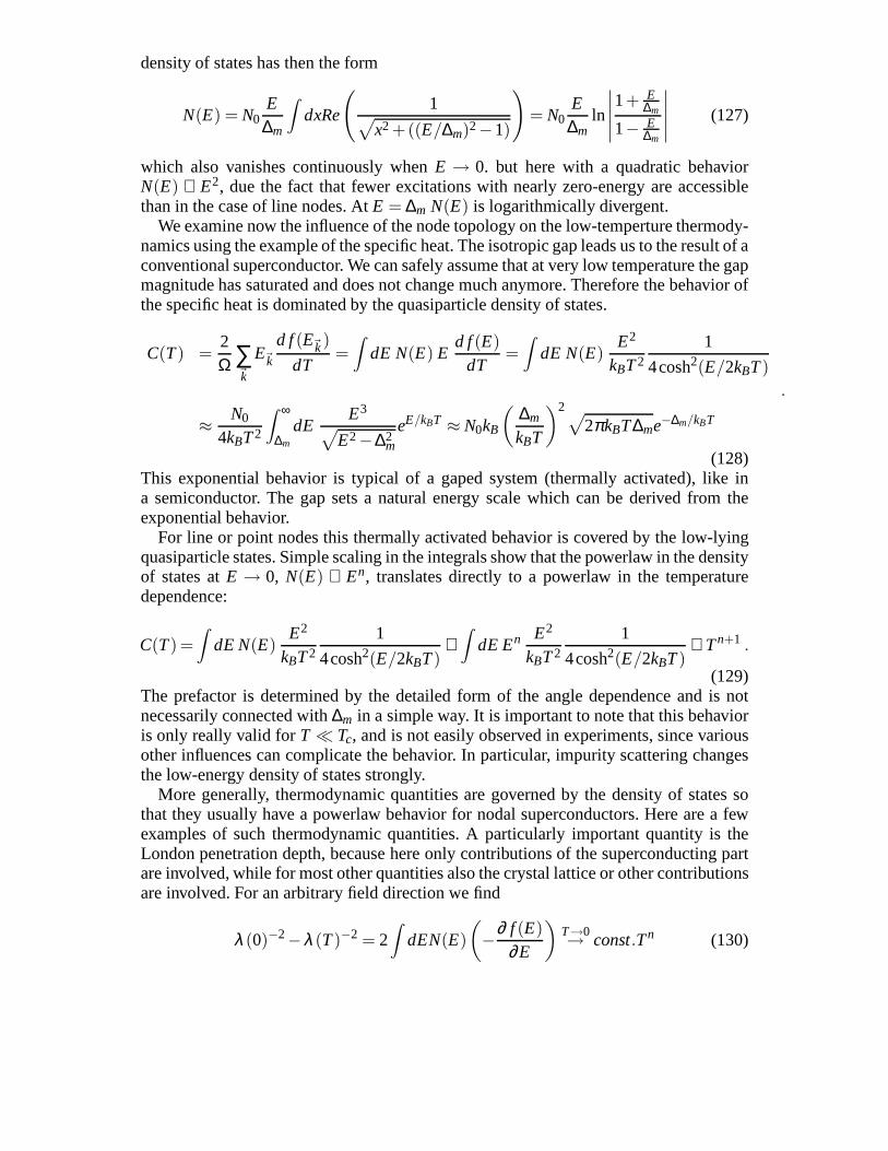
Quantity Line nodes Point nodes

spec. heatC(T) T2 T3

London penetration lengthλ (T)−λ (0) T (T3) T2 (T4)

NMR 1/T1 T3 T5

heat conductivityκ(T) T2 T3

ultrasound absorptionα(T) T (T3) T2 (T4)

Items withTa (Tb) are direction dependent and possess different powerlaws dependingon the orientation of fields or polarizations of the ultrasound.

Spin Susceptibility

The spin susceptibility provides an excellent means to distinguish between spin sin-glet and spin triplet pairing. In spin singlet superconductors the spin susceptibility issuppressed because Cooper pairs have to be broken up in orderto polarize the electronspins. Spin triplet superconductors are more easily spin polarized since the Cooper pairskeep anS= 1 degree of freedom, at least for certain orientations.

We consider here superconductor were the external magneticfield only couplesthrough Zeeman coupling, i.e. we ignore the orbital coupling which is responsible forMeissner screening. The external magnetic field is chosen tolie along thez-axis:

HZ = −µBHz∑~k

c†~k↑c~k↑−c†

~k↓c~k↓

(131)

We tackle the problem by distinguishing two distinct cases of the gap matrix. First,consider a superconducting state with only off-diagonal gap matrix elements, i. e.∆~k↑↑ =

∆~k↓↓ = 0. This includes both spin-singlet pairing (∆~k↑↓ = −∆~k↓↑) as well as triplet-

pairing (∆~k↑↓ = ∆~k↓↑ ⇒ ~d ‖ zwith equal spin-pairing in thex-y-plane). In this case the

quasiparticles Hamiltonian becomes diagonal

HQP = ∑~k

E~k↑a

†~k↑a~k↑ +E~k↓a

†~k↓a~k↓

(132)

with E~ks =√

ξ 2~k

+ |∆~k |2−sµBHz ands=↑,↓ or +,−. The induced magnetization is

Mz = µB∑~k

〈c†~k↑c~k↑−c†

~k↓c~k↓〉 (133)

with〈c†

~ksc~k s〉 = ∑

s′=±

|u~kss′ |

2 f (E~ks′)+ |v~kss′ |2(1− f (E~ks′)

). (134)

Note that|u~kss′|2 ∝ δss′, |v~kss′|2 ∝ |∆~kss′|2 and|u~k↑↑|2+ |v~k↑↓|2 = 1. It follows that

Mz = µB∑~k

(f (E~k↑)− f (E~k↓)

)Hz→0−→ −2µ2

BHz∑~k

∂ f (E~k)

∂E~k

. (135)

Finally the spin susceptibility reads

χ⊥ =Mz

Hz= 2µ2

BN0

∫ dΩ~k

4π

∫dξ

1

4kBTcosh2(E~k/2kBT)= χP

∫ dΩ~k

4πY(k;T) = χPY(T)

(136)with χP = 2µ2

BN0 the Pauli spin susceptibility of the normal state. The function Y(k;T)

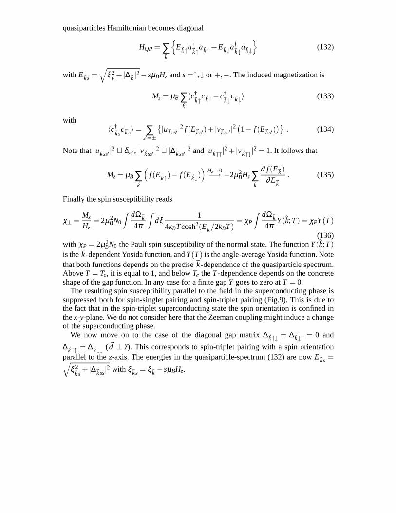
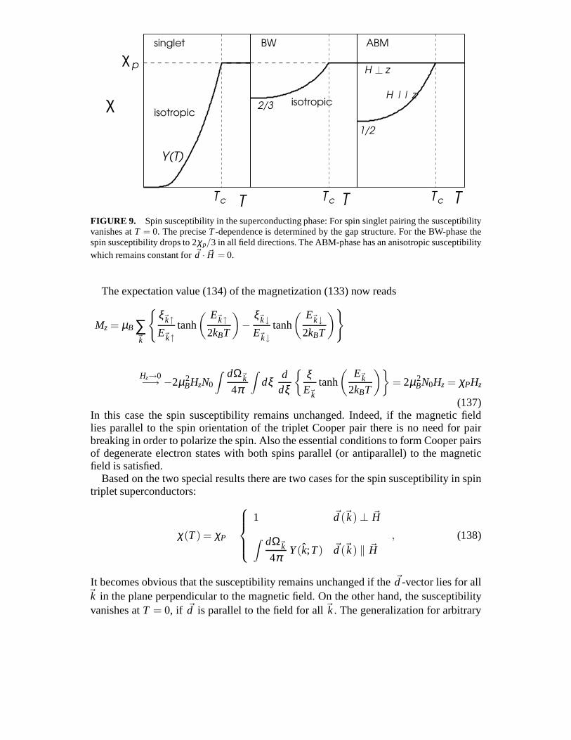
is the~k-dependent Yosida function, andY(T) is the angle-average Yosida function. Notethat both functions depends on the precise~k-dependence of the quasiparticle spectrum.AboveT = Tc, it is equal to 1, and belowTc theT-dependence depends on the concreteshape of the gap function. In any case for a finite gapY goes to zero atT = 0.

The resulting spin susceptibility parallel to the field in the superconducting phase issuppressed both for spin-singlet pairing and spin-tripletpairing (Fig.9). This is due tothe fact that in the spin-triplet superconducting state thespin orientation is confined inthex-y-plane. We do not consider here that the Zeeman coupling might induce a changeof the superconducting phase.

We now move on to the case of the diagonal gap matrix∆~k↑↓ = ∆~k↓↑ = 0 and

∆~k↑↑ = ∆~k↓↓ ( ~d ⊥ z). This corresponds to spin-triplet pairing with a spin orientationparallel to thez-axis. The energies in the quasiparticle-spectrum (132) are nowE~ks =√

ξ 2~ks

+ |∆~kss|2 with ξ~ks= ξ~k −sµBHz.

Y(T)

c Tc Tc

χp

H z

χ

T T T

2/3

1/2

H || zisotropic

isotropic

singlet BW ABM

T

FIGURE 9. Spin susceptibility in the superconducting phase: For spinsinglet pairing the susceptibilityvanishes atT = 0. The preciseT-dependence is determined by the gap structure. For the BW-phase thespin susceptibility drops to 2χp/3 in all field directions. The ABM-phase has an anisotropic susceptibilitywhich remains constant for~d · ~H = 0.

The expectation value (134) of the magnetization (133) now reads

Mz = µB∑~k

ξ~k↑E~k↑

tanh

( E~k↑2kBT

)−

ξ~k↓E~k↓

tanh

( E~k↓2kBT

)

Hz→0−→ −2µ2BHzN0

∫ dΩ~k

4π

∫dξ

ddξ

ξE~k

tanh

(E~k

2kBT

)= 2µ2

BN0Hz = χPHz

(137)In this case the spin susceptibility remains unchanged. Indeed, if the magnetic fieldlies parallel to the spin orientation of the triplet Cooper pair there is no need for pairbreaking in order to polarize the spin. Also the essential conditions to form Cooper pairsof degenerate electron states with both spins parallel (or antiparallel) to the magneticfield is satisfied.

Based on the two special results there are two cases for the spin susceptibility in spintriplet superconductors:

χ(T) = χP

1 ~d(~k) ⊥ ~H

∫ dΩ~k

4πY(k;T) ~d(~k) ‖ ~H

, (138)

It becomes obvious that the susceptibility remains unchanged if the ~d -vector lies for all~k in the plane perpendicular to the magnetic field. On the otherhand, the susceptibilityvanishes atT = 0, if ~d is parallel to the field for all~k. The generalization for arbitrary

fields and spin triplet gap functions yields

χ(T)µν = χP

∫ dΩ~k

4π

δµν −Redµ(~k)∗dν(~k)

| ~d(~k)|2(1−Y(k;T))

(139)

in whichMµ = ∑ν χµνHν .We consider here as a first example the BW-phase for which~d(~k) = ∆0(xkx + yky +

zkz). The calculation by (139) leads to

χBW(T)µν = χPδµν

(1− 1

3(1−Y(T))

). (140)

The spin susceptibilty is isotrop and reaches 2χP/3 for T = 0. A further example is theABM-state for which we have~d(~k) = ∆0z(kx+ iky). In this case the susceptibility reads

χ(T) = χP

YABM(T) ~H ‖ z

1 ~H ⊥ z, (141)

with YABM(T) the Yosida-Function for the ABM-state after integration over the Fermisurface. This phase might be realized in Sr2RuO4 from spin susceptibility measurementsfor fields in thex-y-plane [81].

Obviously it is not only possible to distinguish between spin singlet and spin tripletpairing, but also between different spin triplet state as long as the~d -vector is sufficiently”pinned” due to spin-orbit coupling. The spin susceptibility cannot be measured directlyby the sample magnetization because of Meissner-screening. However, a local probe likenuclear magnetic resonance (NMR) measurements allow us to observe the temperaturedependence of the local susceptibility in the mixed phase (vortex phase) of the supercon-ductor, by looking at the Knight shift, the shift of resonance lines in the NMR spectrum[41]. Similar measurements are also possible with muon spinrelaxation.

The Paramagnetic Limit

The response to Zeeman coupling can play an important role insuperconductors withvery short coherence lengthsξ0 = hvf /π|∆|. The coherence length can be viewed as theextension of the Cooper pairs. The upper critical fieldHc2 due to the orbital depairingdepends onξ0 in the following way

Hc2 =Φ0

2πξ 20

(142)

so thatHc2 can acquire large values for smallξ0. If this is the case depairing due toZeeman spin splitting can become decisive for the destruction of the superconductivity.This phenomenon is called paramagnetic limiting (or Pauli-, Chandrasker- or Clogston-limiting). The paramagnetic limiting field is connected with the spin susceptibility in the

following way. We have to compare the superconducting condensation energy with themagnetization energy which could be reached by the application of a magnetic field:

EZ = −12 ∑

µ,ν(χPδµν −χ(T)µν)HµHν ⇔ Econd = −N0

2|∆m|2〈|g~k |

2〉~k,FS

(143)where we have restricted the comparison toT = 0 andχp = 2µ2

BN0. For spin-singletsuperconductors, we immediately find that a critical field where the two energies areidentical.

Hp =1

µB√

2|∆m|

√〈|g~k |2〉~k,FS . (144)

Thus forHc2 > Hp superconductivity would break down atH = Hp, actually as a dis-continuous first order transition unlike the second order transition for orbital depairingat Hc2. This condition onHc2 is generally quite restrictive, so that it is generally not soeasy to find superconductors displaying paramagnetic limiting.

If paramagnetic limiting is absent, it can be taken as a sign for spin triplet pairing.However, the effect is field direction dependent in general,since the magnetic energy

EZ = −χP

2Re

⟨dµ(~k)∗dν(~k)

| ~d(~k)|2

⟩

~k,FS

HµHν , (145)

has to be compared with the condensation energy. For instance the the ABM-phasediscussed earlier would not be paramagnetically limited for fields in thex-y plane.

PHENOMENOLOGICAL THEORY AND SYMMETRIES

The description of superconductivity based on the theory ofphase transition byGinzburg-Landau is one of the corner stones of our phenomenological understanding ofsuperconductivity in general. The particular strength of this phenomenological theorylies in its generality allowing a formulation even without any detailed microscopicunderstanding of a superconductor. The key quantity is theorder parameterdescribingthe superconducting phase. This order parameter vanishes in the normal state,T > Tc,and grows continuously from zero belowTc. The crucial aspect of the Ginzburg-Landautheory lies in the concept of spontaneous symmetry breakingat a (continuous) secondorder phase transition. This suggests to base the theory on symmetrical grounds which isa powerful strategy as we will show below. The fundamental symmetry to be broken inthe superconducting phase isU(1)-gauge symmetry. This suggests an order parameterwhich would change under the operation ofΦ ∈U(1). While this is the only importantsymmetry for conventional superconductors, we will see below that time reversal andpoint group symmetry of a crystal can also appear in general as broken symmetries inunconventional superconductors [42, 43]

Conventional Superconductors

In order to introduce some basic concepts, it is useful to study first the Ginzburg-Landau phenomenology of conventional superconductors. One choice for the orderparameter is the gap function∆ = −gb~k which indeed changes underU(1)-gaugeoperation by a phase and becomes continuously finite belowTc. Alternatively we couldchooseb~k itsself as the pair wavefunction. In any case we define an order parameterηas∆ = η(~r ,T) as a space and temperature dependent complex wavefunction describingthe superconducting condensate (related also with the density of coherent Cooper pairs).This order parameter changes under basic symmetries as

time reversal : Kη = η∗

U(1) gauge : Φη = ηeiφ(146)

where the vector potential and the electron field operators change under gauge transfor-mation as

Ψ(~r ) , ~A(~r ) ⇔ Ψ(~r )eieχ(~r )/hc , ~A(~r )+ ~∇ χ(~r ) (147)

with φ = 2ieχ/hc, sinceη ∝ 〈ΨΨ〉. Consequently a finite order parameter picks a certainphase which can be changed byU(1)-gauge transformation, breaking this symmetry.

Following Landau we expand the free energy aroundTc in the order parameterη.The free energy is a scalar under symmetry operations belonging to the groupG =K ×U(1). The most general form including the possibility of spatialvariations of theorder parameter is given by

F[η, ~A;T] =∫

Ωd3r

[a(T)|η|2+b(T)|η|4+K(T)|~Πη|2 +

18π

(~∇ × ~A)2]

, (148)

with~Π =

hi~∇ +

2ec

~A . (149)

the canonical ”momentum” (gradient) of the Cooper pairs of charge 2e. Only powers ofη∗η appear which are invariant under time reversal as well asU(1)-gauge operations.We stop the expansion at fourth order. The third term describes the stiffness of the orderparameter against spatial modulations and contains the minimal coupling between theorder parameter and the vector potential and giving this term a gauge invariant form.This term reflects one of the important consequences of a state with brokenU(1)-gaugesymmetry as we will see below. Finally the last term is the magnetic field energy. Thecoefficients are

a(T) ≈ a′(T −Tc) , a′ > 0 , b(T) ≈ b(Tc) = b > 0 and K(T) ≈ K(Tc) = K > 0(150)

so thata(T) changes sign atT = Tc andF is bound towards negative values. For giventemperature we find the equilibrium state by minimizing the free energy variationallywith respect toη and~A.

We discuss first the uniform superconducting phase ignoringspatial variations and themagnetic field:

0 =∂F∂η∗ = a(T)η +2bη|η|2 ⇒ |η|2 =

0 T > Tc

−a(T)

2bT ≤ Tc

(151)

The order parameter satisfies the requirement to be only non-zero belowTc and to growcontinuously from zero. We can now use this solution to calculate some thermodynamicquantities such as entropy and specific heat:

−S=dFdT

= −Sn+ |η|2 dadT

+∂F∂η

dηdT

+∂F∂η∗

dη∗

dT︸ ︷︷ ︸=0

,

C = TdSdT

≈Cn+a′Td|η|2dT

⇒ ∆C|T=Tc = C−Cn|T=Tc =a′2

2b=

8π2k2BTcN0

7ζ (3)Ω .

(152)Using the specific heat result we can related the ratioa/b to the microscopic parameter.The latest enables us to relatea′2/b to the microscopic parameters of the BCS theory.Assuming that the order parameter corresponds to the gap we can derive the coefficientsas

a′ = ΩN0

Tcand b = Ω

7ζ (3)N0

16π2k2BT2

c. (153)

Now we turn to the general inhomogenous form of the order parameter and the vectorpotential. The given expansion of the free energy is valid for variations of the orderparameter on length scales much longer the zero-temperature coherence lengthξ0. Thevariational minimization of the free energy with respect toboth η and ~A leads to theGinzburg-Landau equations

aη +2bη|η|2−K~Π∗ · ~Πη = 0

2ec

K

η∗~Πη +η ~Π ∗η∗− 1

4π~∇ × (~∇ × ~A) = 0

(154)

The second equation can be rewritten as the stationary Maxwell equations which linkscurrent and magnetic field

~∇ × ~B =4πc

2eK

η∗~Πη +η ~Π ∗η∗

=4πc

~j , (155)

with ~j as the supercurrent. For a uniform order parameter|η|, this equation can besimplified into an equation for the magnetic field only

~∇ × (~∇ × ~B) = −4πc

8e2

cK|η|2~B ⇒ ~∇2~B =

1

λ 2L

~B , (156)

which is the London equation describing the screening of themagnetic field. This isan essential consequence of the brokenU(1)-gauge symmetry and corresponds to theHiggs-mechanism in gauge field theories making gauge fields massive by violatinggauge symmetries. A result of the London equation is that an external magnetic fieldcan only penetrate a sample on lengthλL, the London penetration length:

λ−2L =

32πe2

c2 K|η|2 =4πe2ns

mc2 (157)

where the second equality gives the standard form ofλL with ns as the superfluid density.Note thatns is the electronic densityne at T = 0. Near the phase transition one finds

ns(T) = 2ne

(1− T

Tc

)=

7ζ (3)ne

8(πkBTc)2 |η|2 , (158)

which relatesK to microscopic parameters

K =7ζ (3)ne

64πm(πkBTc)2 . (159)

There is a second important length scale in the Ginzburg-Landau equation, the coherencelengthξ . We look at the terms of the first equation in (154), which are linear in the orderparameter. Here we can defineξ naturally as a characteristic length.

(a(T)−Kh2~∇2

)η = a(T)

1−ξ 2~∇2

η

⇒ ξ (T)2 = − h2Ka(T)

=h2K

2b|η|2 =h2v2

F

8π|η|2 ∝Tc

Tc−T,

(160)

which we may compare with coherence lengthξ0 = hvF/π|∆| at T = 0.

Generalization to unconventional order parameters

The extension of the phenomenological theory to general superconducting orderparameters requires to include further symmetries of the system. This leads us to theclassification of the possible order parameters in terms of the irreducible representationsof the corresponding symmetry group analogous to the stationary states in quantummechanics. In the standard case the second order phase transition can be restricted to asingle representation.

To explain this point we consider again the linearized gap equations we had derivedealier for spin singlet and spin triplet pairing with the gapfunctionsψ(~k) and ~d(~k),respectively.

−λψ(~k) = −N0〈vs~k,~k ′ψ(~k ′)〉~k ′,FS for spin singlet pairing

−λ ~d(~k) = −N0〈vt~k,~k ′

~d(~k ′)〉~k ′,FS for spin triplet pairing(161)

where all symmetries are incorporated in the pairing interaction. This is an eigenvalueproblem which gives possible transition temperturesTc. The largest one defines thereal physical instability temperature of the normal state.This corresponds here to thelargest eigenvalueλ . The eigenfunctions belong to irreducible representations whosedimensionality gives the degeneracy of a given eigenvalue.We have shown in theprevious chapter how the gap functions is transformed undersymmetry operations.These operations include besides the time reversal and theU(1)-gauge symmetry alsothe orbital and the spin rotation. In solids the orbital rotation is limited to the point groupoperation of the crystal lattice. Thus we will not be allowedto use the relative angularmomentuml to label the irreducible representations ofSO(3). We will also assume thatspin-orbit coupling is sufficiently strong, so that one can consider the spin to be ”frozen”to the lattice and rotate together with the orbital rotations.

We now would like to construct a free energy that describes a phase transition toan unconventional superconducting phase. Following Landau’s recipe we pick the gapfunction with the highestTc and decompose in the independent basis functions of thisrepresentation,ψm(~k) or ~dm(~k):

ψ(~k) = ∑l

ηmψm(~k) and ~d(~k) = ∑l

ηm~dm(~k) . (162)

where the sum runs over all basis functions of the relevant irreducible representation. It isthus assumed that all other representations have sufficiently lower critical temperaturesto be ignored safely. We will use the coefficientsηm as order parameters in the freeenergy. The free energyF must be real and a scalar functional of the general orderparameterηm and also of the vector potential so it is denotedF[ηm, ~A;T], with T thetemperature parameter. Allηm transform under symmetry operations like coordinatesin the basis of functionsψm(~k) or ~dm(~k), and transform asη → η∗ (η → eiφ η)under time-reversal (U(1)-gauge) operation. The generic form of the scalerF is givenby

F[ηm, ~A;T] = Fn(T)+∫

d3r

a∑

m|ηm|2 + ∑

m1,···,m4

bm1,···,m4η∗m1

η∗m2

ηm3ηm4

+ ∑m1,m2

∑n1,n2

Km1m2,n1n2 (Πn1ηm1)∗ (Πn2ηm2)+

18π

(~∇ × ~A)2

(163)

where

a = a′(T −Tc) , a′,bm,Kmm′,nn′ > 0 and ~Π = ~∇ + i2ehc

~A , (164)

andFn(T) the normal state free energy, which will omitted from now on.The parametersare chosen to satisfy the symmetry condition. The importantmerit of this formulationis that the we can formulate this theory based on a few material dependent parameterswhich should be determined either experimentally or derived from a microscopic theory.This theory goes beyond the weak-coupling approach we had used in the previouschapter and is therefore more general.

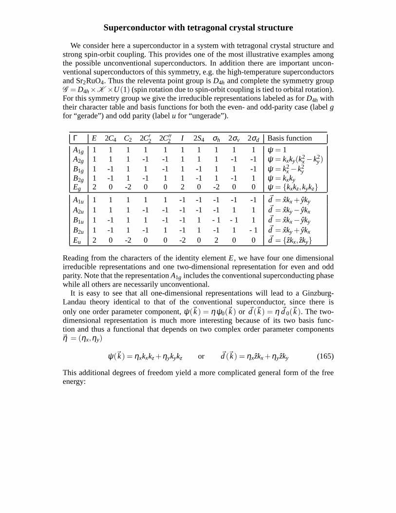
Superconductor with tetragonal crystal structure

We consider here a superconductor in a system with tetragonal crystal structure andstrong spin-orbit coupling. This provides one of the most illustrative examples amongthe possible unconventional superconductors. In additionthere are important uncon-ventional superconductors of this symmetry, e.g. the high-temperature superconductorsand Sr2RuO4. Thus the releventa point group isD4h and complete the symmetry groupG = D4h×K ×U(1) (spin rotation due to spin-orbit coupling is tied to orbitalrotation).For this symmetry group we give the irreducible representations labeled as forD4h withtheir character table and basis functions for both the even-and odd-parity case (labelgfor “gerade”) and odd parity (labelu for “ungerade”).

Γ E 2C4 C2 2C′2 2C′′

2 I 2S4 σh 2σv 2σd Basis function

A1g 1 1 1 1 1 1 1 1 1 1 ψ = 1A2g 1 1 1 -1 -1 1 1 1 -1 -1 ψ = kxky(k2

x −k2y)

B1g 1 -1 1 1 -1 1 -1 1 1 -1 ψ = k2x −k2

yB2g 1 -1 1 -1 1 1 -1 1 -1 1 ψ = kxkyEg 2 0 -2 0 0 2 0 -2 0 0 ψ = kxkz,kykzA1u 1 1 1 1 1 -1 -1 -1 -1 -1 ~d = xkx + yky

A2u 1 1 1 -1 -1 -1 -1 -1 1 1 ~d = xky− ykx

B1u 1 -1 1 1 -1 -1 1 - 1 - 1 1 ~d = xkx− yky

B2u 1 -1 1 -1 1 -1 1 -1 1 - 1 ~d = xky + ykx

Eu 2 0 -2 0 0 -2 0 2 0 0 ~d = zkx, zky

Reading from the characters of the identity elementE, we have four one dimensionalirreducible representations and one two-dimensional representation for even and oddparity. Note that the representationA1g includes the conventional superconducting phasewhile all others are necessarily unconventional.

It is easy to see that all one-dimensional representations will lead to a Ginzburg-Landau theory identical to that of the conventional superconductor, since there isonly one order parameter component,ψ(~k) = ηψ0(~k) or ~d(~k) = η ~d0(~k). The two-dimensional representation is much more interesting because of its two basis func-tion and thus a functional that depends on two complex order parameter components~η = (ηx,ηy)

ψ(~k) = ηxkxkz+ηykykz or ~d(~k) = ηxzkx +ηyzky (165)

This additional degrees of freedom yield a more complicatedgeneral form of the freeenergy:

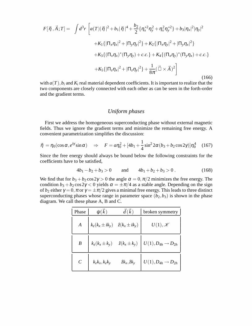
F[~η , ~A;T] =

∫d3r

[a(T)|~η |2+b1|~η |4+

b2

2η∗2

x η2y +η2

x η∗2y +b3|ηx|2|ηy|2

+K1|Πxηx|2+ |Πyηy|2+K2|Πxηy|2+ |Πyηx|2

+K3(Πxηx)∗(Πyηy)+c.c.+K4(Πxηy)

∗(Πyηx)+c.c.

+K5|Πzηx|2+ |Πzηy|2+1

8π(~∇ × ~A)2

]

(166)with a(T),bi andKi real material dependent coefficients. It is important to realize that thetwo components are closely connected with each other as can be seen in the forth-orderand the gradient terms.

Uniform phases

First we address the homogeneous superconducting phase without external magneticfields. Thus we ignore the gradient terms and minimize the remaining free energy. Aconvenient parametrization simplifies the discussion:

~η = η0(cosα,eiγ sinα) ⇒ F = aη20 +[4b1+

14

sin22α(b3+b2cos2γ)]η40 (167)

Since the free energy should always be bound below the following constraints for thecoefficients have to be satisfied,

4b1−b2 +b3 > 0 and 4b1+b2 +b3 > 0 . (168)

We find that forb3 +b2cos2γ > 0 the angleα = 0,π/2 minimizes the free energy. Theconditionb3 +b2cos2γ < 0 yieldsα = ±π/4 as a stable angle. Depending on the signof b2 eitherγ = 0,π or γ =±π/2 gives a minimal free energy. This leads to three distinctsuperconducting phases whose range in parameter space(b2,b3) is shown in the phasediagram. We call these phase A, B and C.

Phase ψ(~k) ~d(~k) broken symmetry

A kz(kx± iky) z(kx± iky) U(1),K

B kz(kx±ky) z(kx±ky) U(1),D4h → D2h

C kzkx,kzky zkx, zky U(1),D4h → D2h

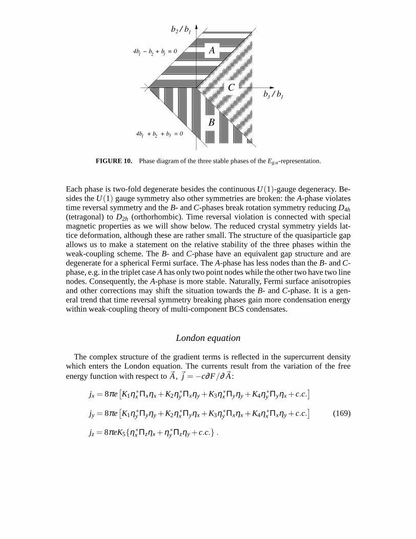
b / b2 1

b / b13

4b + b + b = 01 2 3

4b − b + b = 01 2 3

A

C

B

FIGURE 10. Phase diagram of the three stable phases of theEg,u-representation.

Each phase is two-fold degenerate besides the continuousU(1)-gauge degeneracy. Be-sides theU(1) gauge symmetry also other symmetries are broken: theA-phase violatestime reversal symmetry and theB- andC-phases break rotation symmetry reducingD4h(tetragonal) toD2h (orthorhombic). Time reversal violation is connected withspecialmagnetic properties as we will show below. The reduced crystal symmetry yields lat-tice deformation, although these are rather small. The structure of the quasiparticle gapallows us to make a statement on the relative stability of thethree phases within theweak-coupling scheme. TheB- andC-phase have an equivalent gap structure and aredegenerate for a spherical Fermi surface. TheA-phase has less nodes than theB- andC-phase, e.g. in the triplet caseAhas only two point nodes while the other two have two linenodes. Consequently, theA-phase is more stable. Naturally, Fermi surface anisotropiesand other corrections may shift the situation towards theB- andC-phase. It is a gen-eral trend that time reversal symmetry breaking phases gainmore condensation energywithin weak-coupling theory of multi-component BCS condensates.

London equation

The complex structure of the gradient terms is reflected in the supercurrent densitywhich enters the London equation. The currents result from the variation of the freeenergy function with respect to~A, ~j = −c∂F/∂ ~A:

jx = 8πe[K1η∗

x Πxηx +K2η∗y Πxηy +K3η∗

x Πyηy +K4η∗y Πyηx +c.c.

]

jy = 8πe[K1η∗

y Πyηy +K2η∗x Πyηx +K3η∗

y Πxηx +K4η∗x Πxηy +c.c.

]

jz = 8πeK5η∗x Πzηx +η∗

y Πzηy +c.c. .

(169)

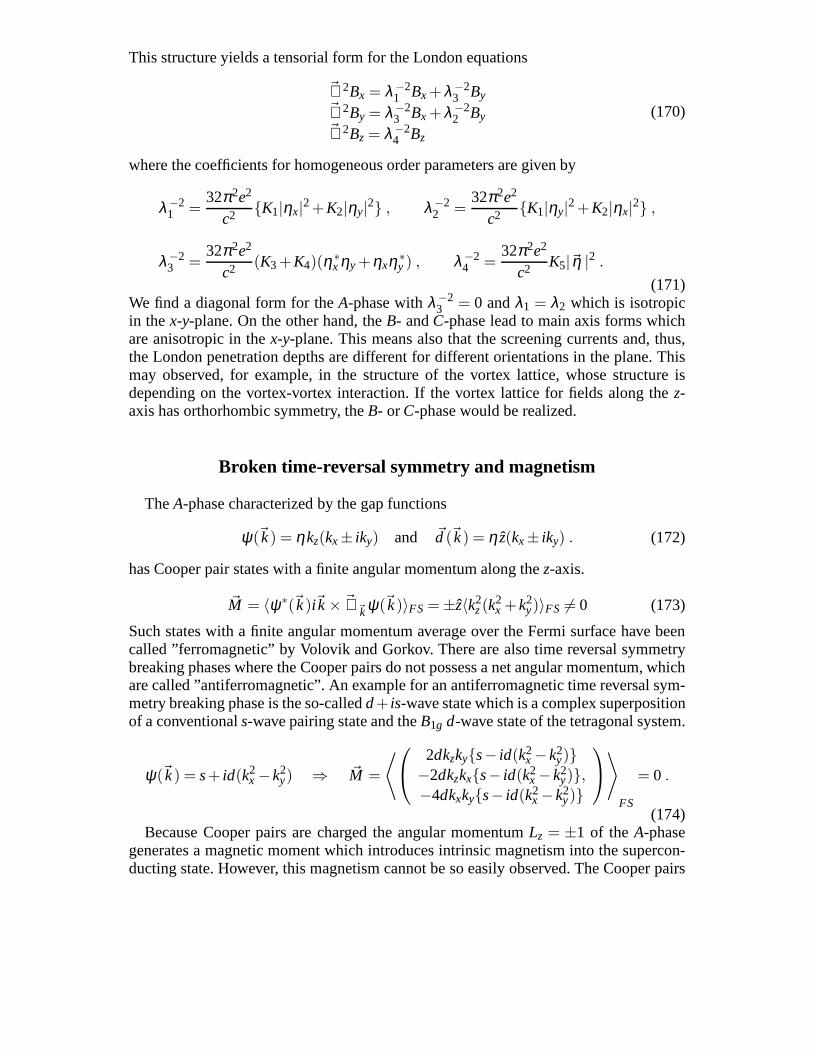
This structure yields a tensorial form for the London equations

~∇2Bx = λ−21 Bx +λ−2

3 By~∇2By = λ−2

3 Bx +λ−22 By

~∇2Bz = λ−24 Bz

(170)

where the coefficients for homogeneous order parameters aregiven by

λ−21 =

32π2e2

c2 K1|ηx|2+K2|ηy|2 , λ−22 =

32π2e2

c2 K1|ηy|2+K2|ηx|2 ,

λ−23 =

32π2e2

c2 (K3+K4)(η∗x ηy +ηxη∗

y ) , λ−24 =

32π2e2

c2 K5|~η |2 .

(171)We find a diagonal form for theA-phase withλ−2

3 = 0 andλ1 = λ2 which is isotropicin thex-y-plane. On the other hand, theB- andC-phase lead to main axis forms whichare anisotropic in thex-y-plane. This means also that the screening currents and, thus,the London penetration depths are different for different orientations in the plane. Thismay observed, for example, in the structure of the vortex lattice, whose structure isdepending on the vortex-vortex interaction. If the vortex lattice for fields along thez-axis has orthorhombic symmetry, theB- or C-phase would be realized.

Broken time-reversal symmetry and magnetism

TheA-phase characterized by the gap functions

ψ(~k) = ηkz(kx± iky) and ~d(~k) = η z(kx± iky) . (172)

has Cooper pair states with a finite angular momentum along thez-axis.

~M = 〈ψ∗(~k)i~k × ~∇~kψ(~k)〉FS = ±z〈k2z(k

2x +k2

y)〉FS 6= 0 (173)

Such states with a finite angular momentum average over the Fermi surface have beencalled ”ferromagnetic” by Volovik and Gorkov. There are also time reversal symmetrybreaking phases where the Cooper pairs do not possess a net angular momentum, whichare called ”antiferromagnetic”. An example for an antiferromagnetic time reversal sym-metry breaking phase is the so-calledd+ is-wave state which is a complex superpositionof a conventionals-wave pairing state and theB1g d-wave state of the tetragonal system.

ψ(~k) = s+ id(k2x −k2

y) ⇒ ~M =

⟨

2dkzkys− id(k2

x −k2y)

−2dkzkxs− id(k2x −k2

y),−4dkxkys− id(k2

x −k2y)

⟩

FS

= 0 .

(174)Because Cooper pairs are charged the angular momentumLz = ±1 of theA-phase

generates a magnetic moment which introduces intrinsic magnetism into the supercon-ducting state. However, this magnetism cannot be so easily observed. The Cooper pairs

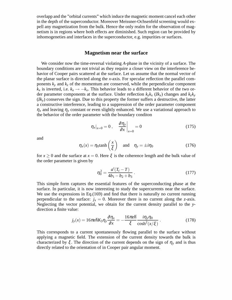
overlapp and the ”orbital currents” which induce the magnetic moment cancel each otherin the depth of the superconductor. Moreover Meissner-Ochsenfeld screening would ex-pell any magnetization from the bulk. Hence the only realm for the observation of mag-netism is in regions where both effects are diminished. Suchregion can be provided byinhomogeneties and interfaces in the superconductor, e.g.impurities or surfaces.

Magnetism near the surface

We consider now the time-reversal violatingA-phase in the vicinity of a surface. Theboundary conditions are not trivial as they require a closerview on the interference be-havior of Cooper pairs scattered at the surface. Let us assume that the normal vector ofthe planar surface is directed along thex-axis. For specular reflection the parallel com-ponentsky andkz of the momentum are conserved, while the perpendicular componentkx is inverted, i.e.kx → −kx. This behavior leads to a different behavior of the two or-der parameter components at the surface. Under reflectionkzkx (zkx) changes andkzky(zky) conserves the sign. Due to this property the former suffersa destructive, the lattera constructive interference, leading to a suppression of the order parameter componentηx and leavingηy constant or even slightly enhanced. We use a variational approach tothe behavior of the order parameter with the boundary conditon

ηx|x=0 = 0 ,∂ηy

∂x

∣∣∣∣x=0

= 0 (175)

and

ηx(x) = η0tanh

(xξ

)and ηy = ±iη0 (176)

for x≥ 0 and the surface atx = 0. Hereξ is the coherence length and the bulk value ofthe order parameter is given by

η20 =

a′(Tc−T)

4b1−b2+b3. (177)

This simple form captures the essential features of the superconducting phase at thesurface. In particular, it is now interesting to study the supercurrents near the surface.We use the expressions in Eq.(169) and find that there is naturally no current runningperpendicular to the surface:jx = 0. Moreover there is no current along thez-axis.Neglecting the vector potential, we obtain for the current density parallel to they-direction a finite value:

jy(x) = 16πehK3ηy∂ηx

∂x= −16πeh

ξiηyη0

cosh2(x/ξ ). (178)

This corresponds to a current spontaneously flowing parallel to the surface withoutapplying a magnetic field. The extension of the current density towards the bulk ischaracterized byξ . The direction of the current depends on the sign ofηy and is thusdirectly related to the orientation of in Cooper pair angular moment.

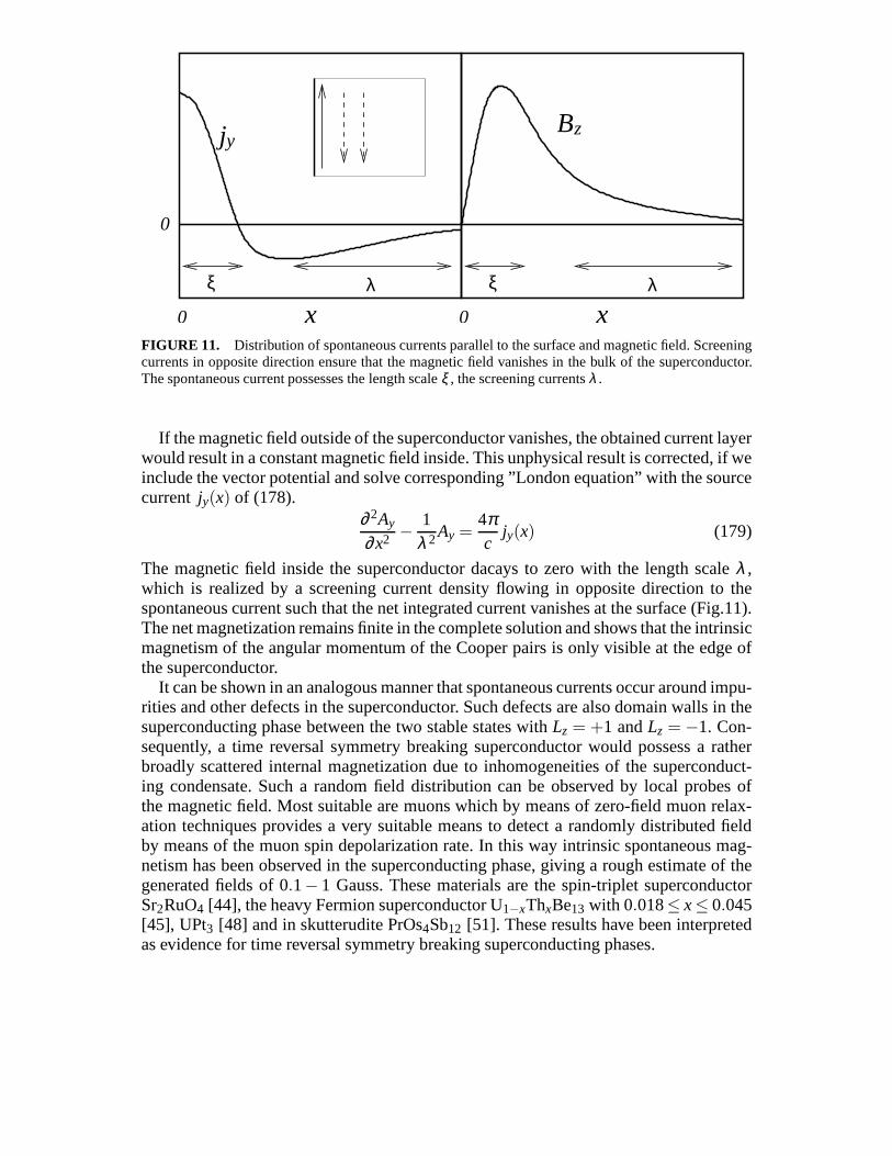
ξ λ ξ λ

jy Bz

0 0x x

0

FIGURE 11. Distribution of spontaneous currents parallel to the surface and magnetic field. Screeningcurrents in opposite direction ensure that the magnetic field vanishes in the bulk of the superconductor.The spontaneous current possesses the length scaleξ , the screening currentsλ .

If the magnetic field outside of the superconductor vanishes, the obtained current layerwould result in a constant magnetic field inside. This unphysical result is corrected, if weinclude the vector potential and solve corresponding ”London equation” with the sourcecurrent jy(x) of (178).

∂ 2Ay

∂x2 − 1λ 2Ay =

4πc

jy(x) (179)

The magnetic field inside the superconductor dacays to zero with the length scaleλ ,which is realized by a screening current density flowing in opposite direction to thespontaneous current such that the net integrated current vanishes at the surface (Fig.11).The net magnetization remains finite in the complete solution and shows that the intrinsicmagnetism of the angular momentum of the Cooper pairs is onlyvisible at the edge ofthe superconductor.

It can be shown in an analogous manner that spontaneous currents occur around impu-rities and other defects in the superconductor. Such defects are also domain walls in thesuperconducting phase between the two stable states withLz = +1 andLz = −1. Con-sequently, a time reversal symmetry breaking superconductor would possess a ratherbroadly scattered internal magnetization due to inhomogeneities of the superconduct-ing condensate. Such a random field distribution can be observed by local probes ofthe magnetic field. Most suitable are muons which by means of zero-field muon relax-ation techniques provides a very suitable means to detect a randomly distributed fieldby means of the muon spin depolarization rate. In this way intrinsic spontaneous mag-netism has been observed in the superconducting phase, giving a rough estimate of thegenerated fields of 0.1− 1 Gauss. These materials are the spin-triplet superconductorSr2RuO4 [44], the heavy Fermion superconductor U1−xThxBe13 with 0.018≤ x≤ 0.045[45], UPt3 [48] and in skutterudite PrOs4Sb12 [51]. These results have been interpretedas evidence for time reversal symmetry breaking superconducting phases.

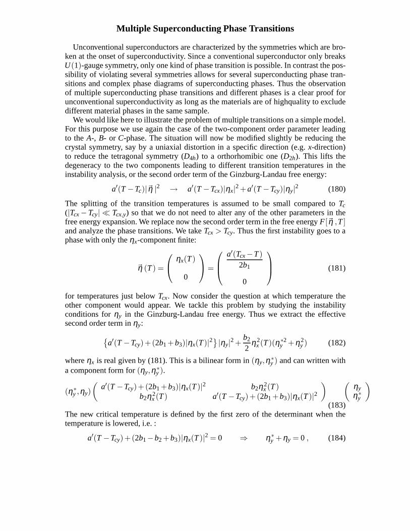
Multiple Superconducting Phase Transitions

Unconventional superconductors are characterized by the symmetries which are bro-ken at the onset of superconductivity. Since a conventionalsuperconductor only breaksU(1)-gauge symmetry, only one kind of phase transition is possible. In contrast the pos-sibility of violating several symmetries allows for several superconducting phase tran-sitions and complex phase diagrams of superconducting phases. Thus the observationof multiple superconducting phase transitions and different phases is a clear proof forunconventional superconductivity as long as the materialsare of highquality to excludedifferent material phases in the same sample.

We would like here to illustrate the problem of multiple transitions on a simple model.For this purpose we use again the case of the two-component order parameter leadingto theA-, B- or C-phase. The situation will now be modified slightly be reducing thecrystal symmetry, say by a uniaxial distortion in a specific direction (e.g.x-direction)to reduce the tetragonal symmetry (D4h) to a orthorhomibic one (D2h). This lifts thedegeneracy to the two components leading to different transition temperatures in theinstability analysis, or the second order term of the Ginzburg-Landau free energy:

a′(T −Tc)|~η |2 → a′(T −Tcx)|ηx|2+a′(T −Tcy)|ηy|2 (180)

The splitting of the transition temperatures is assumed to be small compared toTc(|Tcx−Tcy| Tcx,y) so that we do not need to alter any of the other parameters in thefree energy expansion. We replace now the second order term in the free energyF[~η ,T]and analyze the phase transitions. We takeTcx > Tcy. Thus the first instability goes to aphase with only theηx-component finite:

~η (T) =

ηx(T)

0

=

a′(Tcx−T)

2b1

0

(181)

for temperatures just belowTcx. Now consider the question at which temperature theother component would appear. We tackle this problem by studying the instabilityconditions forηy in the Ginzburg-Landau free energy. Thus we extract the effectivesecond order term inηy:

a′(T −Tcy)+(2b1+b3)|ηx(T)|2

|ηy|2+

b2

2η2

x (T)(η∗2y +η2

y ) (182)

whereηx is real given by (181). This is a bilinear form in(ηy,η∗y ) and can written with

a component form for(ηy,η∗y ).

(η∗y ,ηy)

(a′(T −Tcy)+(2b1+b3)|ηx(T)|2 b2η2

x (T)b2η2

x (T) a′(T −Tcy)+(2b1+b3)|ηx(T)|2) (

ηyη∗

y

)

(183)The new critical temperature is defined by the first zero of thedeterminant when thetemperature is lowered, i.e. :

a′(T −Tcy)+(2b1−b2+b3)|ηx(T)|2 = 0 ⇒ η∗y +ηy = 0 , (184)

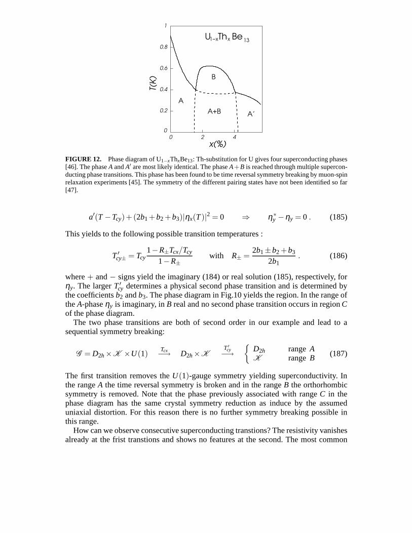
1−x

0

0.2

0.4

0.6

0.8

1

0 2 4

A

B

A+B A’

x(%)T(

K)

U Th Be13x

FIGURE 12. Phase diagram of U1−xThxBe13: Th-substitution for U gives four superconducting phases[46]. The phaseA andA′ are most likely identical. The phaseA+B is reached through multiple supercon-ducting phase transitions. This phase has been found to be time reversal symmetry breaking by muon-spinrelaxation experiments [45]. The symmetry of the differentpairing states have not been identified so far[47].

a′(T −Tcy)+(2b1+b2+b3)|ηx(T)|2 = 0 ⇒ η∗y −ηy = 0 . (185)

This yields to the following possible transition temperatures :

T ′cy± = Tcy

1−R±Tcx/Tcy

1−R±with R± =

2b1±b2 +b3

2b1. (186)

where+ and− signs yield the imaginary (184) or real solution (185), respectively, forηy. The largerT ′

cy determines a physical second phase transition and is determined bythe coefficientsb2 andb3. The phase diagram in Fig.10 yields the region. In the range oftheA-phaseηy is imaginary, inB real and no second phase transition occurs in regionCof the phase diagram.

The two phase transitions are both of second order in our example and lead to asequential symmetry breaking:

G = D2h×K ×U(1)Tcx−→ D2h×K

T ′cy−→

D2h rangeAK rangeB (187)

The first transition removes theU(1)-gauge symmetry yielding superconductivity. Inthe rangeA the time reversal symmetry is broken and in the rangeB the orthorhombicsymmetry is removed. Note that the phase previously associated with rangeC in thephase diagram has the same crystal symmetry reduction as induce by the assumeduniaxial distortion. For this reason there is no further symmetry breaking possible inthis range.

How can we observe consecutive superconducting transtions? The resistivity vanishesalready at the frist transtions and shows no features at the second. The most common

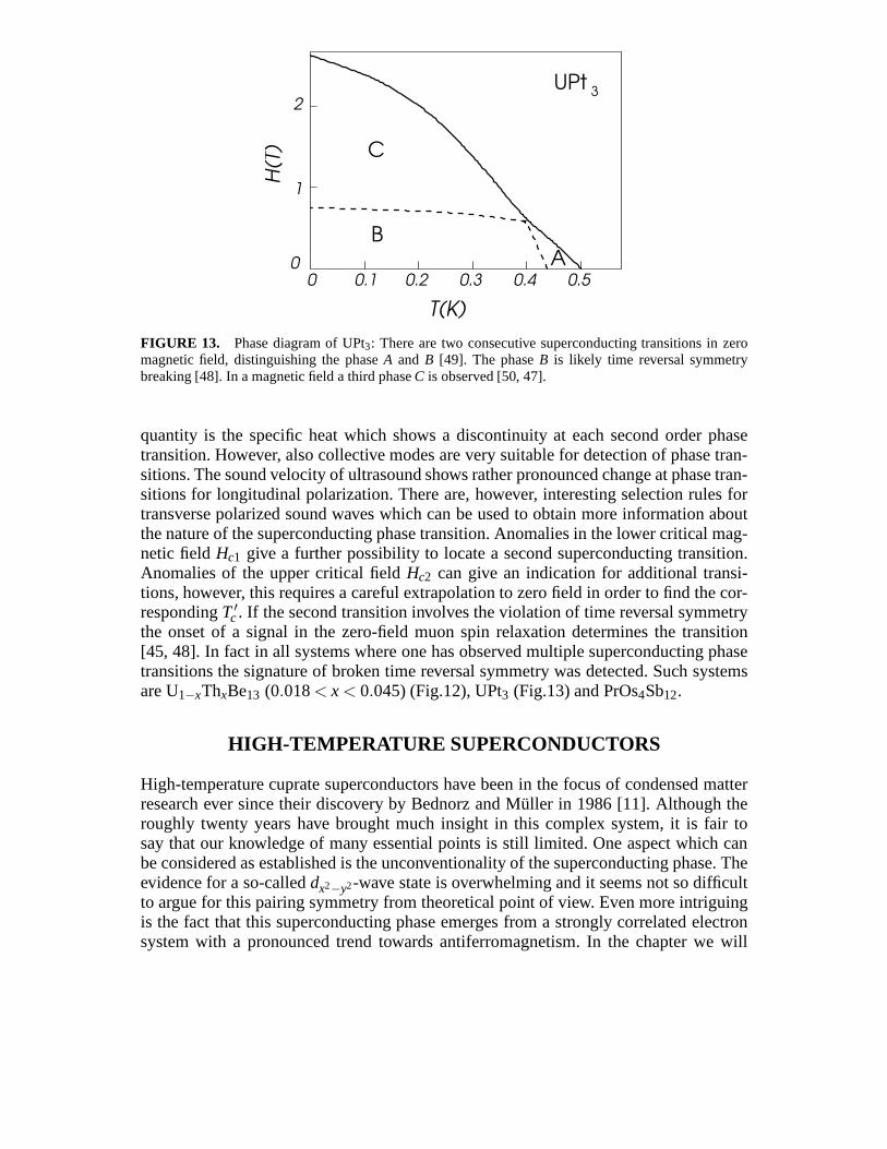
A

3

0 0.1 0.2 0.3 0.4 0.50

1

2

H(T

)

T(K)

C

B

UPt

FIGURE 13. Phase diagram of UPt3: There are two consecutive superconducting transitions inzeromagnetic field, distinguishing the phaseA and B [49]. The phaseB is likely time reversal symmetrybreaking [48]. In a magnetic field a third phaseC is observed [50, 47].

quantity is the specific heat which shows a discontinuity at each second order phasetransition. However, also collective modes are very suitable for detection of phase tran-sitions. The sound velocity of ultrasound shows rather pronounced change at phase tran-sitions for longitudinal polarization. There are, however, interesting selection rules fortransverse polarized sound waves which can be used to obtainmore information aboutthe nature of the superconducting phase transition. Anomalies in the lower critical mag-netic fieldHc1 give a further possibility to locate a second superconducting transition.Anomalies of the upper critical fieldHc2 can give an indication for additional transi-tions, however, this requires a careful extrapolation to zero field in order to find the cor-respondingT ′

c. If the second transition involves the violation of time reversal symmetrythe onset of a signal in the zero-field muon spin relaxation determines the transition[45, 48]. In fact in all systems where one has observed multiple superconducting phasetransitions the signature of broken time reversal symmetrywas detected. Such systemsare U1−xThxBe13 (0.018< x < 0.045) (Fig.12), UPt3 (Fig.13) and PrOs4Sb12.

HIGH-TEMPERATURE SUPERCONDUCTORS

High-temperature cuprate superconductors have been in thefocus of condensed matterresearch ever since their discovery by Bednorz and Müller in1986 [11]. Although theroughly twenty years have brought much insight in this complex system, it is fair tosay that our knowledge of many essential points is still limited. One aspect which canbe considered as established is the unconventionality of the superconducting phase. Theevidence for a so-calleddx2−y2-wave state is overwhelming and it seems not so difficultto argue for this pairing symmetry from theoretical point ofview. Even more intriguingis the fact that this superconducting phase emerges from a strongly correlated electronsystem with a pronounced trend towards antiferromagnetism. In the chapter we will

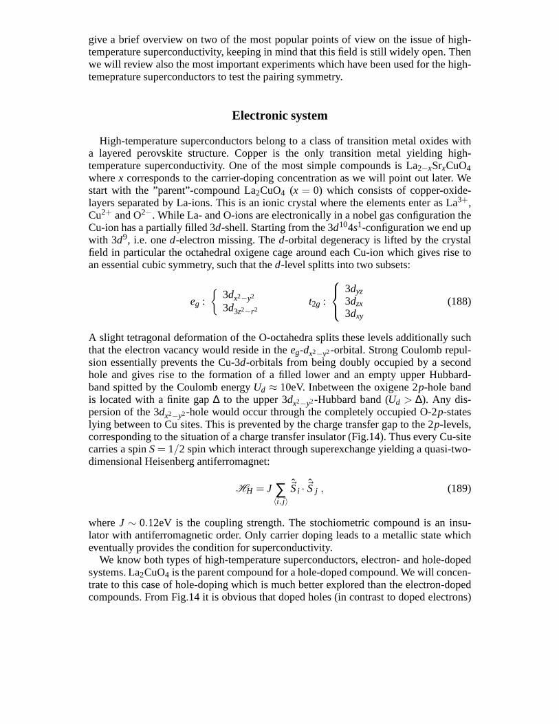
give a brief overview on two of the most popular points of viewon the issue of high-temperature superconductivity, keeping in mind that this field is still widely open. Thenwe will review also the most important experiments which have been used for the high-temeprature superconductors to test the pairing symmetry.

Electronic system

High-temperature superconductors belong to a class of transition metal oxides witha layered perovskite structure. Copper is the only transition metal yielding high-temperature superconductivity. One of the most simple compounds is La2−xSrxCuO4wherex corresponds to the carrier-doping concentration as we willpoint out later. Westart with the ”parent”-compound La2CuO4 (x = 0) which consists of copper-oxide-layers separated by La-ions. This is an ionic crystal where the elements enter as La3+,Cu2+ and O2−. While La- and O-ions are electronically in a nobel gas configuration theCu-ion has a partially filled 3d-shell. Starting from the 3d104s1-configuration we end upwith 3d9, i.e. oned-electron missing. Thed-orbital degeneracy is lifted by the crystalfield in particular the octahedral oxigene cage around each Cu-ion which gives rise toan essential cubic symmetry, such that thed-level splitts into two subsets:

eg :

3dx2−y2

3d3z2−r2t2g :

3dyz3dzx3dxy

(188)

A slight tetragonal deformation of the O-octahedra splits these levels additionally suchthat the electron vacancy would reside in theeg-dx2−y2-orbital. Strong Coulomb repul-sion essentially prevents the Cu-3d-orbitals from being doubly occupied by a secondhole and gives rise to the formation of a filled lower and an empty upper Hubbard-band spitted by the Coulomb energyUd ≈ 10eV. Inbetween the oxigene 2p-hole bandis located with a finite gap∆ to the upper 3dx2−y2-Hubbard band (Ud > ∆). Any dis-persion of the 3dx2−y2-hole would occur through the completely occupied O-2p-stateslying between to Cu sites. This is prevented by the charge transfer gap to the 2p-levels,corresponding to the situation of a charge transfer insulator (Fig.14). Thus every Cu-sitecarries a spinS= 1/2 spin which interact through superexchange yielding a quasi-two-dimensional Heisenberg antiferromagnet:

HH = J ∑〈i, j〉

~Si · ~S j , (189)

whereJ ∼ 0.12eV is the coupling strength. The stochiometric compound is an insu-lator with antiferromagnetic order. Only carrier doping leads to a metallic state whicheventually provides the condition for superconductivity.

We know both types of high-temperature superconductors, electron- and hole-dopedsystems. La2CuO4 is the parent compound for a hole-doped compound. We will concen-trate to this case of hole-doping which is much better explored than the electron-dopedcompounds. From Fig.14 it is obvious that doped holes (in contrast to doped electrons)

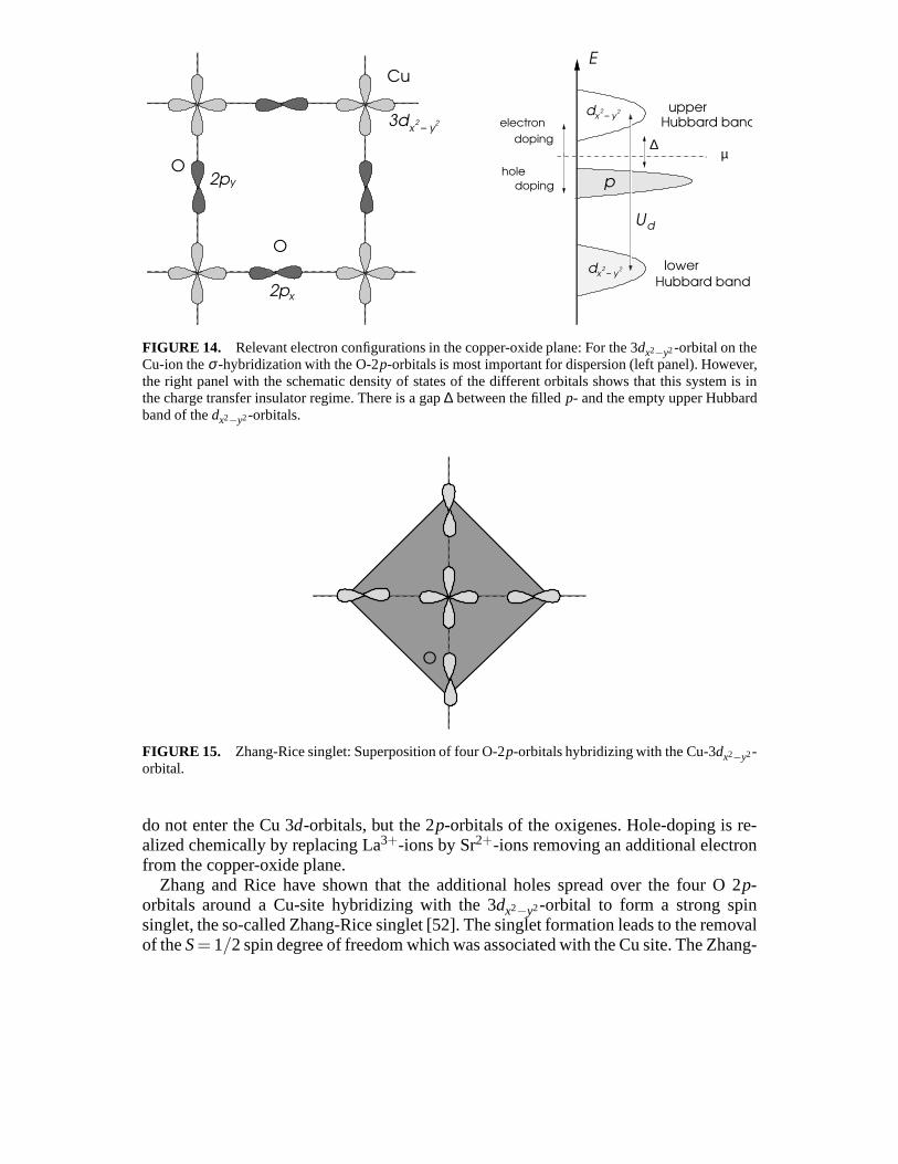
Hubbard band

Hubbard band

hole

doping

electron

doping

µ

upper

lower

E

x − y223d

2py

2px

x − y22d

x − y22d

Cu

O

O

p

∆

dU

FIGURE 14. Relevant electron configurations in the copper-oxide plane: For the 3dx2−y2-orbital on theCu-ion theσ -hybridization with the O-2p-orbitals is most important for dispersion (left panel). However,the right panel with the schematic density of states of the different orbitals shows that this system is inthe charge transfer insulator regime. There is a gap∆ between the filledp- and the empty upper Hubbardband of thedx2−y2-orbitals.

O

FIGURE 15. Zhang-Rice singlet: Superposition of four O-2p-orbitals hybridizing with the Cu-3dx2−y2-orbital.

do not enter the Cu 3d-orbitals, but the 2p-orbitals of the oxigenes. Hole-doping is re-alized chemically by replacing La3+-ions by Sr2+-ions removing an additional electronfrom the copper-oxide plane.

Zhang and Rice have shown that the additional holes spread over the four O 2p-orbitals around a Cu-site hybridizing with the 3dx2−y2-orbital to form a strong spinsinglet, the so-called Zhang-Rice singlet [52]. The singlet formation leads to the removalof theS= 1/2 spin degree of freedom which was associated with the Cu site. The Zhang-

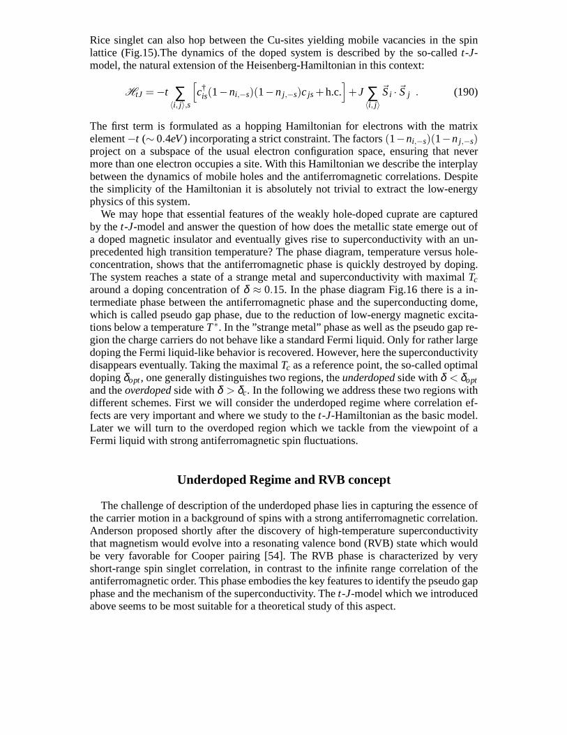
Rice singlet can also hop between the Cu-sites yielding mobile vacancies in the spinlattice (Fig.15).The dynamics of the doped system is described by the so-calledt-J-model, the natural extension of the Heisenberg-Hamiltonian in this context:

HtJ = −t ∑〈i, j〉,s

[c†

is(1−ni,−s)(1−n j ,−s)c js +h.c.]+J ∑

〈i, j〉~Si · ~S j . (190)

The first term is formulated as a hopping Hamiltonian for electrons with the matrixelement−t (∼ 0.4eV) incorporating a strict constraint. The factors(1−ni,−s)(1−n j ,−s)project on a subspace of the usual electron configuration space, ensuring that nevermore than one electron occupies a site. With this Hamiltonian we describe the interplaybetween the dynamics of mobile holes and the antiferromagnetic correlations. Despitethe simplicity of the Hamiltonian it is absolutely not trivial to extract the low-energyphysics of this system.

We may hope that essential features of the weakly hole-dopedcuprate are capturedby thet-J-model and answer the question of how does the metallic stateemerge out ofa doped magnetic insulator and eventually gives rise to superconductivity with an un-precedented high transition temperature? The phase diagram, temperature versus hole-concentration, shows that the antiferromagnetic phase is quickly destroyed by doping.The system reaches a state of a strange metal and superconductivity with maximal Tcaround a doping concentration ofδ ≈ 0.15. In the phase diagram Fig.16 there is a in-termediate phase between the antiferromagnetic phase and the superconducting dome,which is called pseudo gap phase, due to the reduction of low-energy magnetic excita-tions below a temperatureT∗. In the ”strange metal” phase as well as the pseudo gap re-gion the charge carriers do not behave like a standard Fermi liquid. Only for rather largedoping the Fermi liquid-like behavior is recovered. However, here the superconductivitydisappears eventually. Taking the maximalTc as a reference point, the so-called optimaldopingδopt, one generally distinguishes two regions, theunderdopedside withδ < δoptand theoverdopedside withδ > δc. In the following we address these two regions withdifferent schemes. First we will consider the underdoped regime where correlation ef-fects are very important and where we study to thet-J-Hamiltonian as the basic model.Later we will turn to the overdoped region which we tackle from the viewpoint of aFermi liquid with strong antiferromagnetic spin fluctuations.

Underdoped Regime and RVB concept

The challenge of description of the underdoped phase lies incapturing the essence ofthe carrier motion in a background of spins with a strong antiferromagnetic correlation.Anderson proposed shortly after the discovery of high-temperature superconductivitythat magnetism would evolve into a resonating valence bond (RVB) state which wouldbe very favorable for Cooper pairing [54]. The RVB phase is characterized by veryshort-range spin singlet correlation, in contrast to the infinite range correlation of theantiferromagnetic order. This phase embodies the key features to identify the pseudo gapphase and the mechanism of the superconductivity. Thet-J-model which we introducedabove seems to be most suitable for a theoretical study of this aspect.

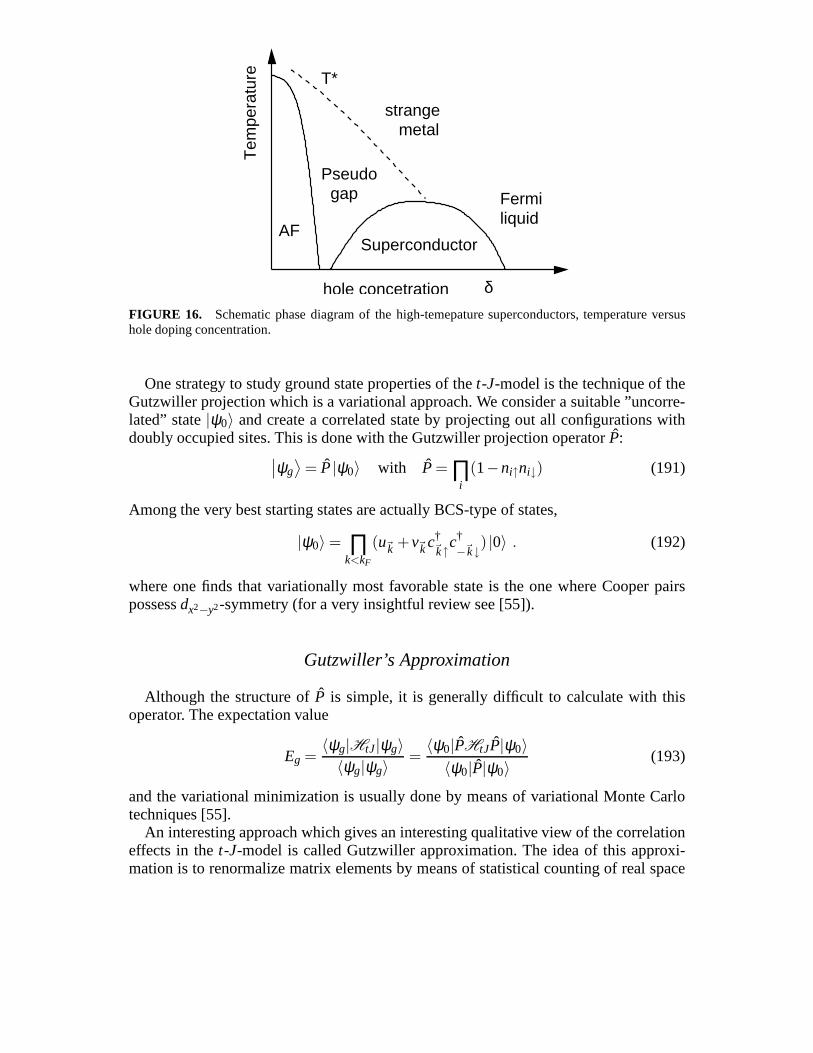
liquidAF

Fermi

δ

T*

Pseudo gap

strange metal

Tem

pera

ture

hole concetration

Superconductor

FIGURE 16. Schematic phase diagram of the high-temepature superconductors, temperature versushole doping concentration.

One strategy to study ground state properties of thet-J-model is the technique of theGutzwiller projection which is a variational approach. We consider a suitable ”uncorre-lated” state|ψ0〉 and create a correlated state by projecting out all configurations withdoubly occupied sites. This is done with the Gutzwiller projection operatorP:

∣∣ψg⟩

= P|ψ0〉 with P = ∏i

(1−ni↑ni↓) (191)

Among the very best starting states are actually BCS-type ofstates,

|ψ0〉 = ∏k<kF

(u~k +v~kc†~k↑c

†−~k↓) |0〉 . (192)

where one finds that variationally most favorable state is the one where Cooper pairspossessdx2−y2-symmetry (for a very insightful review see [55]).

Gutzwiller’s Approximation

Although the structure ofP is simple, it is generally difficult to calculate with thisoperator. The expectation value

Eg =〈ψg|HtJ|ψg〉〈ψg|ψg〉

=〈ψ0|PHtJP|ψ0〉

〈ψ0|P|ψ0〉(193)

and the variational minimization is usually done by means ofvariational Monte Carlotechniques [55].

An interesting approach which gives an interesting qualitative view of the correlationeffects in thet-J-model is called Gutzwiller approximation. The idea of thisapproxi-mation is to renormalize matrix elements by means of statistical counting of real space

configurations. Thus the fully correlated HamiltonianHtJ will be replaced by an effec-tive Hamiltonian without constraints.

HG = −gtt ∑〈i, j〉,s

[c†

isc js +h.c.]−µ ∑

i,sni,s+gJJ ∑

〈i, j〉~Si · ~S j . (194)

Renormalization factorsgt and gJ are determined by comparing the constrained andunconstraint expectation values:

⟨c†

isc js

⟩= gt

⟨c†

isc js

⟩

0hopping (195)

⟨~Si · ~S j

⟩= gJ

⟨~Si · ~S j

⟩

0spin exchange (196)

⟨c†

i↑c†j↓

⟩= g∆

⟨c†

i↑c†j↓

⟩

0pairing (197)

with 〈· · ·〉 the expectation values in the constrained Hamiltonian and〈· · ·〉0 the expecta-tion values in the unconstrained Hamiltonian. Moreover, a pairing renormalization factorg∆ is introduced in order to discuss the renormalization of thepairing gap even thoughit does not explicitly appear in the renormalized Hamiltonian.

First we considergt for the particle hopping:

〈ψ|c†isc js|ψ〉 = gt 〈ϕ0|c†

isc js |ϕ0〉 (198)

where|ψ〉 is a state where all configurations of double occupancy are absent, while|ϕ0〉is an uncorrelated state with|ψ〉 ↔√

gt |ϕ0〉. Only states with one particle on sitej andnone on sitei are relevant in|ψ〉 so that we approximategt through the comparison ofconfigurational probabilities:

P(↑,0)+P(↓,0) = gt [P0(↑,0)+P0(↓,0)] . (199)

HereP andP0 are the probabilities for constraint and unconstraint configurations, re-spectively. The left-hand side is the density of electron multiplying the density of holesn(1−n). The right-hand side reads

P0(↑,0)+P0(↓,0) =⟨ni↑(1−n j↑)

⟩0 +⟨ni↓(1−n j↓)

⟩0 = 〈ni〉0−

⟨ni↑n j↑

⟩0−⟨ni↓n j↓

⟩0

(200)which yields approximativelyn−n2/4−n2/4, since electrons are supposed to be un-correlated. Then,gt results as

gt ≈2(1−n)

2−n(201)

The same reasoning can be done for the exchange renormalization parameter. Now wehave ∣∣s,s′

⟩↔√

gJ∣∣s,s′

⟩0 . (202)

Since the process involves two electrons, exactly one on twoneighboring sites, theprobabilities of configurations give

∑s,s′

P(s,s′) = gJ∑s,s′

P0(s,s′) . (203)

The left-hand side isn2. For electrons on neighboring sitesi and j, the right-hand side is

∑s,s′

⟨ni,s(1−ni,−s)n j ,s′(1−n j ,−s′)

⟩0 =

⟨nin j

⟩0−2

⟨nin j↑n j↓

⟩0+4

⟨ni↑ni↓n j↑n j↓

⟩0 .

(204)This is approximated asn2−2n(n/2)2+4(n/2)4 = (2−n)2n2/4 so that

gJ ≈4

(2−n)2 (205)

Finally we consider the renormalization of the pairing amplitudes,g∆. This is an off-diagonal expectation value which couples states with different total number of electrons.Thus the matrix elements take the form

〈ψ(N)|c†i↑c

†j↓ |ψ(N−2)〉 = g∆ 〈ϕ0(N)|c†

i↑c†j↓ |ϕ0(N−2)〉 ⇔ (206)

|ψ(N)〉 → γN |ϕ0(N)〉 and |ψ(N−2)〉 → γN−2 |ϕ0(N−2)〉 , (207)

with g∆ = γNγN−2. The probabilities of the relevant configurations are

P(↑,↓) =n2

4= γ2

NP0(↑,↓) = γ2N〈ni↑n j↓〉0 = γ2

Nn2

4(208)

so thatγN = 1. In the same way we evaluate

P(0,0) = (1−n)2 = γ2N−2P0(0,0) = γ2

N−2

⟨(1−ni↑)(1−n j↓)

⟩= γ2

N−2

(1− n

2

)2,

(209)leading toγN−2 = 2(1−n)/(2−n) such that

g∆ =2(1−n)

2−n= gt , (210)

Both hopping and pairing are connected with the quasiparticle weight of the electrons atthe Fermi surface, which is reduced through the correlationeffects. We find that bothgtandg∆ vanish as we approach half-filling,n → 1. It is obvious that the charge fluctua-tions under the constraint would be suppressed giving rise to increasing difficulties forhopping due to the lack of free sites. In much the same way the BCS pairing is relyingon the availability on configurations with unoccupied sites. On the other hand, we findthatgJ takes its maximal (enhanced) value at half filling, since this yields with securityconfiguration where neighboring sites are occupied by just single electrons.

Mean field treatment

The Fermionic operators which we use inHG are now not constraint anymore andwithin our approximation the effect of projections is incorportated by the renormaliza-tion factors. Nevertheless, we are still confronted with a many-body problem which we

would like to tackle by means of a mean field ansatz to decouplethe Heisenberg partof HG. It turns out that the following two types of mean fields are giving a descriptionwhich carries the idea obtained from the above variational treatment:

χi j =⟨

c†isc js

⟩

0and ∆i j =

⟨c†

i↑c†j↓

⟩

0, (211)

whereχi j is a hopping mean field and∆i j is a BCS-like pairing mean field. Note that weneglect here the staggered magnetic moment as another obvious mean field. These arenearest-neighbor mean fields which are considered to be unform throughout the systemwith

χi,i+ax = χx , χi,i+ay = χy , ∆i,i+ax = ∆x , ∆i,i+ay = ∆y . (212)

The transformation to momentum space leads to the followingeffective (one-particle)mean field Hamiltonian

HMF = ∑~k,s

ξ~kc†~k,s

c~k,s−∑~k

∆∗

~kc~k↓c~k↑ +h.c.

+

3Jgj

2 ∑~k

∣∣χ~k

∣∣2+∣∣∆~k

∣∣2

(213)

with

ξ~k = −2 ∑α=x,y

gtt +gJ

3J4

χα

coskα −µ

= ε~k −µ −gJ3J2 ∑

α=x,yχα coskα (214)

∆~k = −gJ3J2 ∑

α=x,y∆α coskα (215)

andε~k =−2tgt(coskx +cosky). The self-consistence equations lead to a stable solutionwith

χx = χy = χ and ∆x = −∆y = ∆ (216)

for sufficiently low temperatures. The energy spectrum of the Bogolyubov quasiparticlesis given by

E~k = ±√

ξ 2~k

+ |∆~k |2 (217)

with an energy gap. The mean field∆~k has an onset temperatureT∗ which graduallydecreases from a high value at half filling upon increasingδ = 1− n and eventuallyreaches zero aroungδ ∼ 0.3. The onset of the hopping mean field lies higher and has nostraightforward physical interpretation.

Despite the formal analogy the mean field∆~k is not the BCS superconducting orderparameter which we only obtain with proper renormalizationtaking the restricted chargefluctuations into account. We find

∆BCS,~k = g∆∆~k =2(1−n)

2−n∆~k (218)

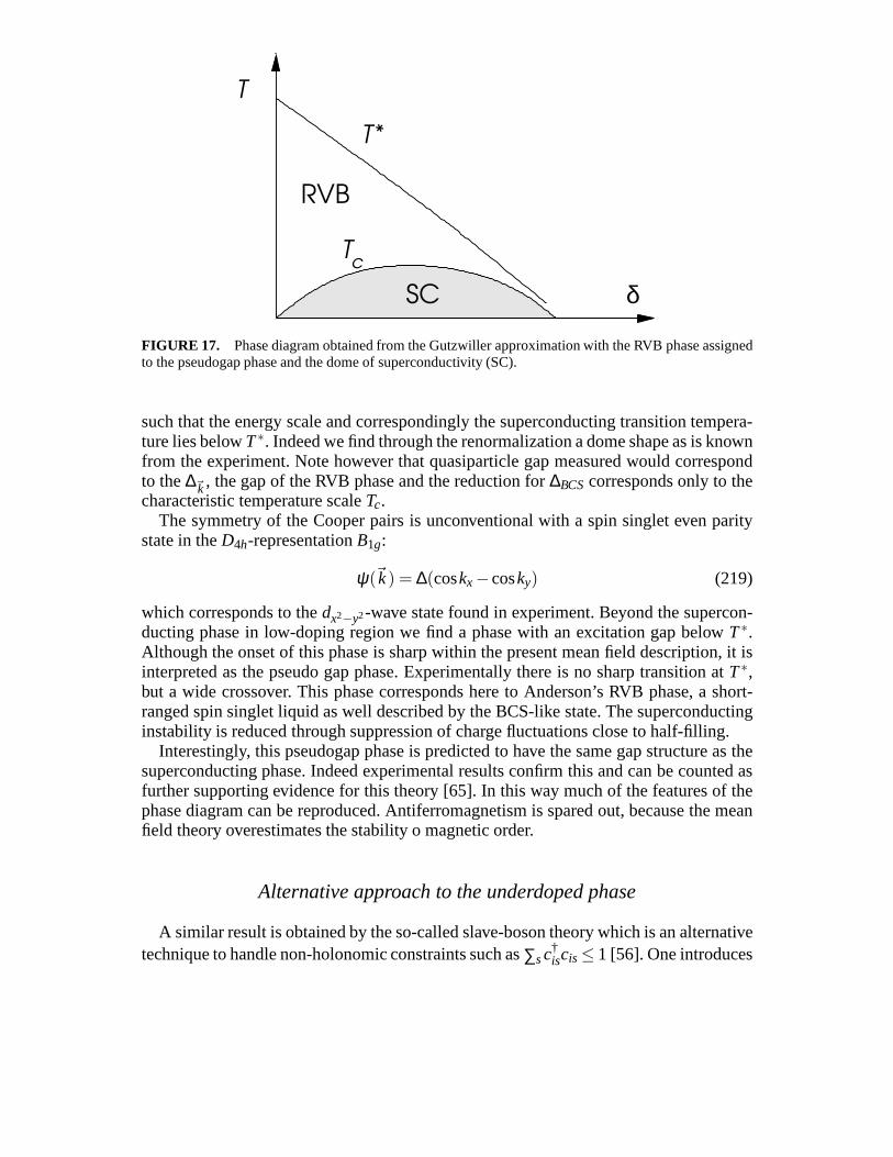
δ

T

T*

RVB

c

SC

T

FIGURE 17. Phase diagram obtained from the Gutzwiller approximation with the RVB phase assignedto the pseudogap phase and the dome of superconductivity (SC).

such that the energy scale and correspondingly the superconducting transition tempera-ture lies belowT∗. Indeed we find through the renormalization a dome shape as isknownfrom the experiment. Note however that quasiparticle gap measured would correspondto the∆~k , the gap of the RVB phase and the reduction for∆BCScorresponds only to thecharacteristic temperature scaleTc.

The symmetry of the Cooper pairs is unconventional with a spin singlet even paritystate in theD4h-representationB1g:

ψ(~k) = ∆(coskx−cosky) (219)

which corresponds to thedx2−y2-wave state found in experiment. Beyond the supercon-ducting phase in low-doping region we find a phase with an excitation gap belowT∗.Although the onset of this phase is sharp within the present mean field description, it isinterpreted as the pseudo gap phase. Experimentally there is no sharp transition atT∗,but a wide crossover. This phase corresponds here to Anderson’s RVB phase, a short-ranged spin singlet liquid as well described by the BCS-likestate. The superconductinginstability is reduced through suppression of charge fluctuations close to half-filling.

Interestingly, this pseudogap phase is predicted to have the same gap structure as thesuperconducting phase. Indeed experimental results confirm this and can be counted asfurther supporting evidence for this theory [65]. In this way much of the features of thephase diagram can be reproduced. Antiferromagnetism is spared out, because the meanfield theory overestimates the stability o magnetic order.

Alternative approach to the underdoped phase

A similar result is obtained by the so-called slave-boson theory which is an alternativetechnique to handle non-holonomic constraints such as∑sc†

iscis ≤ 1 [56]. One introduces

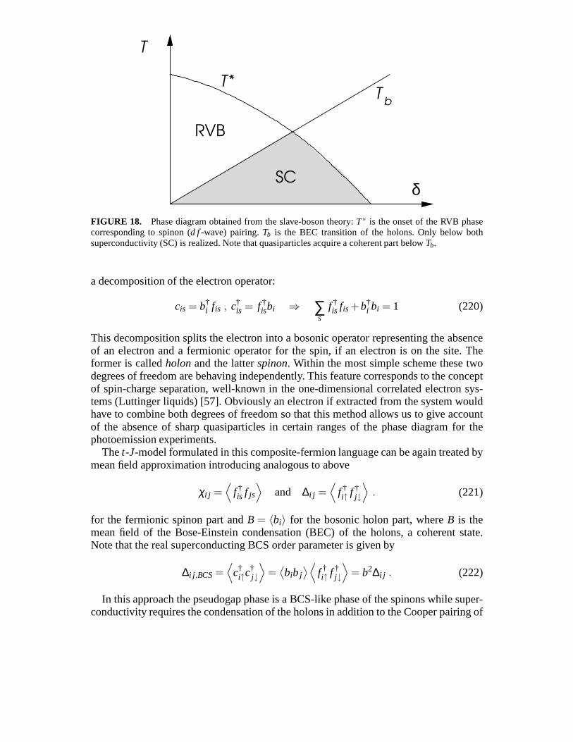
b

SC

RVB

T

T

T*

δ

FIGURE 18. Phase diagram obtained from the slave-boson theory:T∗ is the onset of the RVB phasecorresponding to spinon (d f-wave) pairing.Tb is the BEC transition of the holons. Only below bothsuperconductivity (SC) is realized. Note that quasiparticles acquire a coherent part belowTb.

a decomposition of the electron operator:

cis = b†i fis , c†

is = f †isbi ⇒ ∑

sf †is fis +b†

i bi = 1 (220)

This decomposition splits the electron into a bosonic operator representing the absenceof an electron and a fermionic operator for the spin, if an electron is on the site. Theformer is calledholonand the latterspinon. Within the most simple scheme these twodegrees of freedom are behaving independently. This feature corresponds to the conceptof spin-charge separation, well-known in the one-dimensional correlated electron sys-tems (Luttinger liquids) [57]. Obviously an electron if extracted from the system wouldhave to combine both degrees of freedom so that this method allows us to give accountof the absence of sharp quasiparticles in certain ranges of the phase diagram for thephotoemission experiments.

Thet-J-model formulated in this composite-fermion language can be again treated bymean field approximation introducing analogous to above

χi j =⟨

f †is f js

⟩and ∆i j =

⟨f †i↑ f †

j↓

⟩. (221)

for the fermionic spinon part andB = 〈bi〉 for the bosonic holon part, whereB is themean field of the Bose-Einstein condensation (BEC) of the holons, a coherent state.Note that the real superconducting BCS order parameter is given by

∆i j ,BCS=⟨

c†i↑c

†j↓

⟩=⟨bib j

⟩⟨f †i↑ f †

j↓

⟩= b2∆i j . (222)

In this approach the pseudogap phase is a BCS-like phase of the spinons while super-conductivity requires the condensation of the holons in addition to the Cooper pairing of

the spinons (SC=RVB+BEC) (see Fig.18). Analogous to the Gutzwiller approximationmethod one finds here an RVB phase below a characteristic temperatureT∗ and super-conductivity appears at lower temperature. The holon condensation temperature growslinearly with the hole density, whileT∗ decreases. Where the two temperatures cross wefind the maximalTc (optimal doping). In the overdoped regime we above the supercon-ducting phase no spinon pairing while the holons are condensed. The presence of thecondensate allows to find a coherent part in the electron weight, so that one could inter-pret the normal state here as Fermi liquid-like. The spinon-holon picture is complicatedby the fact that two degrees of freedom are coupled by aU(1)-gauge field. Hence thespin-charge separation is to some extent a spurious featureof the theory [56].

While the RVB-phase gives an elegant interpretation of the underdoped region, it isdifficult to establish this picture firmely. The situation iscomplicated by the fact thatmany different states seem to have comparable energy. Disorder can stabilize phase-separated states leading to the formation of charged stripes in a spin background. Othercandidates have been the flux state or the d-density wave state which could competewith the RVB phase. Another attempt to explain the pseudogapphase is based onan extended region of superconducting fluctuations. Cooperpairs are created at hightemperature but do not form a phase coherent condensate. Each of these proposed phasesand concepts relies on a set of experiments for their support. However, no satisfactorydescription of the emergence of the cuprated physics in the underdoped region out of anantiferromagnetic insulator has been given so far.

Overdoped Regime

In the overdoped regime the normal state properties turn into a more standard metalstate. Thet-J-model of the weakly-doped system is obsolete here and the descriptionin terms of a Fermi liquid phase with rather strong antiferromagnetic spin fluctuationslooks more appropriate. This provides an alternative routeto the description of high-temperature superconductivity, sparing out the complications of the underdoped (al-though there are attempts to extend this kind of analysis into the underdoped region;this is, however, beyond the scope of our lecture) [58]. The starting point is the Hub-bard model in two dimensions from which we may derive an effective spin fluctuationbased interaction between electrons, which is eventually responsible for the formation ofCooper pairs. Alternatively the spin fluctuations can also be introduced as a phenomeno-logical input.

Effective spin fluctuation model

Restricting to the spin fluctuation induced interaction part we can introduce to follow-ing effective Hamiltonian:

Hs f = ∑~k,s

ξ~kc†~ks

c~ks−1

2N2 ∑~k,~k ′,~q

∑s1,s2,s3,s4

v(~q)~σ s1s2 · ~σ s3s4c†~k+~q,s1

c~ks2c†~k ′−~q,s3

c~k ′,s4,

(223)with the band energyξ~k (=−2t(coskx+cosky)−µ for a simple nearest-neighbor tight-binding model),N as the number of sites of the lattice. The effective interaction has theform

v(~q) = U +U2χ(~q) with χ(~q) =χ0(~q)

1−Uχ0(~q). (224)

with the approximative RPA form for the static spin susceptibility χ(~q) whereχ0(~q)is the spin susceptibility of the free electron system. Since we are concerned withthe possibility of Cooper pairing, we ignore all scatteringevents apart form the pairscattering in the Cooper channel. Hence the interaction part of the Hamiltonian reducesto the following terms in which we separate out the spin-singlet and the spin-triplet part:

Hpair =1

N2 ∑~k,~k ′

∑s

Vt

~k,~k′(c†~k,s

c†−~k ,s

c−~k ′,sc~k ′,s+c†~k ,s

c†−~k,−s

c−~k ′,−sc~k ′,s)

+Vs~k,~k ′c

†~k ,s

c†−~k,−s

c−~k ′,−sc~k ′,s

,

(225)

with the spin-triplet and spin-singlet coupling matrix elements,

Vt~k,~k′ = −1

4

[v(~k −~k ′)−v(~k +~k ′)

]resp. Vs

~k,~k ′ =34

[v(~k −~k ′)+v(~k +~k ′)

],

(226)In the sense of the weak-coupling these matrix elements are non-zero only within anenergy region of width 2εc around the Fermi energy. The interaction contains two parts,a repulsive onsite interactionU preventing to pair in the most simples-wave form, anda susceptibility dependent part on which we will focus now. The susceptibility can inpriniciple be calculated in the RPA scheme using the given band structure. Even moresophisticated approaches developed for itinerant electron systems close to magnetictransitions may be applied such as the self-consistent renormalization scheme [53]. Inorder to keep matters simple we assume a simple form for the susceptibility which givesthe essential features of the interaction. We parameterizeχ(~q) as

χ(~q) ≈ χ0[1−b f(~q)] with f = cosqx +cosqy , (227)

This χ(~q) describes antiferromagnetic spin fluctuations, if it is maximal at ~q = ~Q =(π/a,π/a) (a: lattice constant), i.e.b > 0. In contrast, negativeb corresponds to ferro-magnetic spin fluctuations.

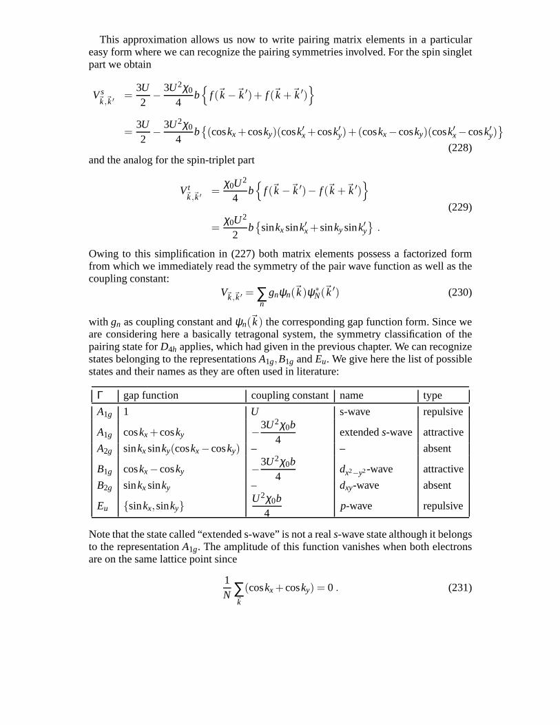
This approximation allows us now to write pairing matrix elements in a particulareasy form where we can recognize the pairing symmetries involved. For the spin singletpart we obtain

Vs~k,~k ′ =

3U2

− 3U2χ0

4b

f (~k −~k ′)+ f (~k +~k ′)

=3U2

− 3U2χ0

4b(coskx +cosky)(cosk′x +cosk′y)+(coskx−cosky)(cosk′x−cosk′y)

(228)and the analog for the spin-triplet part

Vt~k,~k ′ =

χ0U2

4b

f (~k −~k ′)− f (~k +~k ′)

=χ0U2

2b

sinkxsink′x +sinkysink′y

.

(229)

Owing to this simplification in (227) both matrix elements possess a factorized formfrom which we immediately read the symmetry of the pair wave function as well as thecoupling constant:

V~k,~k ′ = ∑n

gnψn(~k)ψ∗N(~k ′) (230)

with gn as coupling constant andψn(~k) the corresponding gap function form. Since weare considering here a basically tetragonal system, the symmetry classification of thepairing state forD4h applies, which had given in the previous chapter. We can recognizestates belonging to the representationsA1g,B1g andEu. We give here the list of possiblestates and their names as they are often used in literature:

Γ gap function coupling constant name type

A1g 1 U s-wave repulsive

A1g coskx +cosky −3U2χ0b4

extendeds-wave attractive

A2g sinkxsinky(coskx−cosky) – – absent

B1g coskx−cosky −3U2χ0b4

dx2−y2-wave attractive

B2g sinkxsinky – dxy-wave absent

Eu sinkx,sinkyU2χ0b

4p-wave repulsive

Note that the state called “extended s-wave” is not a reals-wave state although it belongsto the representationA1g. The amplitude of this function vanishes when both electronsare on the same lattice point since

1N ∑

~k

(coskx +cosky) = 0 . (231)

For antiferromagnetic spin-fluctuations, onlyA1g (extendeds-wave) andB1g pairingstates give rise to an attractive interaction. Both are associated with the spin-singletchannel. (Note that for negativeb, i.e. ferromagnetic spin fluctuations, the representationEu would provide the only channel with attractive interaction.)

We now have to address the instability condition. The linearized gap equation has theform

−λψ(~k) = −〈N0(k)Vs~k,~k′ψ(~k ′)〉~k′,FS (232)

and look for the highest eigenvalueλ (N0(k): angle dependent density of states on theFermi level). It is easy to see that the instability is not only depending on the couplingconstant which is identical for the extendeds-wave and thedx2−y2-wave state, but alsothe gap function form on the Fermi surface plays a role, in particular the Fermi surfaceaverage:

I [ψ] = 〈N0(k)|ψ(~k)|2〉~k,FS . (233)

We find that I [ψA1g] < I [ψB1g], i.e. the leading instability results fromdx2−y2 -wavepairing. It is easy to see that the extendeds-wave state has a small gap function overall the Fermi surface, while thedx2−y2-wave state has nodes along the (11)-direction, butis largest along the(10)- and(01)-direction where the density of state is largest in thetwo-dimensional electron system.

The discussion based on the spin fluctuation based mechanismleads to the same pair-ing state symmetry as the Gutzwiller-approximation for thet-J-model. This consistentresult is not so surprising in view of the fact that the interaction term in thet-J-model isin its structure also a spin fluctuation type of interaction.Moreover the approach (227)leads to the same mathematical structure for both cases. This result is especially satis-factory as the experiments confirm this shape of the pairing interaction.

Testing the Pairing Symmetry

The pairing symmetry has been one of the most important question of the early 1990salso from the experimental point of view. The presence of line nodes constitute oneimportant characteristic feature of thedx2−y2-wave state. These nodes can be approachedby a number of ways. However, the nodes alone do not give the entire picture of the pairwave function. It is also important to establish the phase structure.

Line nodes

The probably first indication for line nodes came from experiments which probe thelow-energy (temperature) quasiparticle spectrum. These were the NMR-1/T1 measure-ments which noted aT3-powerlaw behavior forT → 0 [60]. Moreover aT-linear behav-ior has been seen in the low-temperature London penetrationdepth [61]. Both resultsare compatible with line nodes. The fact that hereTc is extremely high made it naturallyeasier to address these powerlaws experimentally than in most other unconventional su-perconductors.

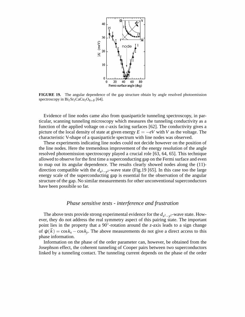
node

FIGURE 19. The angular dependence of the gap structure obtain by angle resolved photoemissionspectroscopy in Bi2Sr2CaCu2O8+δ [64].

Evidence of line nodes came also from quasiparticle tunneling spectroscopy, in par-ticular, scanning tunneling microscopy which measures thetunneling conductivity as afunction of the applied voltage onc-axis facing surfaces [62]. The conductivity gives apicture of the local density of state at given energyE = −eV with V as the voltage. Thecharacteristic V-shape of a quasiparticle spectrum with line nodes was observed.

These experiments indicating line nodes could not decide however on the position ofthe line nodes. Here the tremendous improvement of the energy resolution of the angleresolved photoemission spectroscopy played a crucial role[63, 64, 65]. This techniqueallowed to observe for the first time a superconducting gap onthe Fermi surface and evento map out its angular dependence. The results clearly showed nodes along the (11)-direction compatible with thedx2−y2-wave state (Fig.19 [65]. In this case too the largeenergy scale of the superconducting gap is essential for theobservation of the angularstructure of the gap. No similar measurements for other unconventional superconductorshave been possibile so far.

Phase sensitive tests - interference and frustration

The above tests provide strong experimental evidence for thedx2−y2-wave state. How-ever, they do not address the real symmetry aspect of this pairing state. The importantpoint lies in the property that a 90-rotation around thez-axis leads to a sign changeof ψ(~k) = coskx− cosky. The above measurements do not give a direct access to thisphase information.

Information on the phase of the order parameter can, however, be obtained from theJosephson effect, the coherent tunneling of Cooper pairs between two superconductorslinked by a tunneling contact. The tunneling current depends on the phase of the order

parameter on the two sides of the contact interface:

I = Icsin(φ2−φ1) (234)

whereIc is the maximal current (Josephson coupling) andφ1,2 are the phases of the orderparameter (gap function / pair wave function) on the side 1 and 2, respectively. This stan-dard formula is simple and unproblematic for conventional superconductors. However,in the case of unconventional superconductors geometric aspects of the interface start toplay a role. For thedx2−y2-wave phase the phase of the order parameter is different alongthex- and along they-direction. The phase difference for the two directions isπ . Thus,having contacts on two interfaces,x- andy-oriented, then the their current-phase rela-tion would be shifted byπ . This property has been used to probe this symmetry featurethrough an interference experiment.

We consider the configuration as given in Fig.20 where a conventional superconductoris coupled to adx2−y2-wave superconductor on two orthogonal faces. This is a typicalSQUID (Superconducting QUantum Interference Device) where the flux gives via anAharanov-Bohm-type effect for the Cooper pairs a periodic interference pattern of themaximal current as a function of the magnetic flux threading the SQUID-loop. The totalcurrent through this device consists of the contributions of the two junctions 1 and 2:

I = I1+ I2 = Ic1sinϕ1 + Ic2sin(ϕ2+α) with ϕ1−ϕ2 = 2πΦΦ0

(235)

with Φ0 = hc/2e is the superconducting magnetic flux quantum. The second terminvolves a phase shiftα which is π in the present situation. It is easy to calculate themaximal current assumingIc1 = Ic2 = Ic.

Imax(Φ) = Ic

∣∣∣∣cos

(π

ΦΦ0

+a2

)∣∣∣∣ . (236)

While the standard SQUID (α = 0) shows a maximum forΦ = nΦ0, the configurationwith the d-wave superconductor (α = π) is shifted by half a flux quantum with amaximum for Φ = (n/2+ 1)Φ0 (see Fig.21. This type of experiments have indeedbeen performed in the specified configuration with YBa2Cu3O7 by several groups witha positive result giving an even stronger support for the realization of dx2−y2-wavesymmetry in the cuprate superconductors [70, 71, 72, 66].

Another related experiment addresses the phase frustration effect in a superconductingloop where aπ-shift like this is buildt in. We assume that the superconducting loop doesnot allow any flux to leak out so that enclosed flux is defined by the following condition

0 =∮

d~s ·(

~∇φ − 2πΦ0

~A

)= 2πn+∑

iαi −2π

ΦΦ0

(237)

where the sum runs overall Josephson junction in the loop andαi denotes the phase shift(0,π) (n: integer). Note that these phase shifts are not gauge independent. However,the sum does not change under any gauge transformation in anyof the superconductingsegments along the loop. One always finds∑i αi = πn′, either withn′ an even or an odd

++

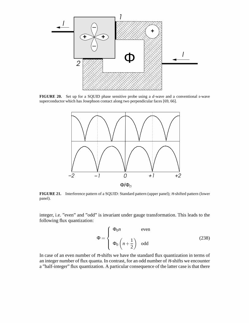
I

I

2

+

1

Φ

FIGURE 20. Set up for a SQUID phase sensitive probe using ad-wave and a conventionals-wavesuperconductor which has Josephson contact along two perpendicular faces [69, 66].

+2

0

0 +1−2 −1

Φ/ΦFIGURE 21. Interference pattern of a SQUID: Standard pattern (upper panel);π-shifted pattern (lowerpanel).

integer, i.e. ”even” and ”odd” is invariant under gauge transformation. This leads to thefollowing flux quantization:

Φ =

Φ0n even

Φ0

(n+

12

)odd

(238)

In case of an even number ofπ-shifts we have the standard flux quantization in terms ofan integer number of flux quanta. In contrast, for an odd number of π-shifts we encountera ”half-integer” flux quantization. A particular consequence of the latter case is that there

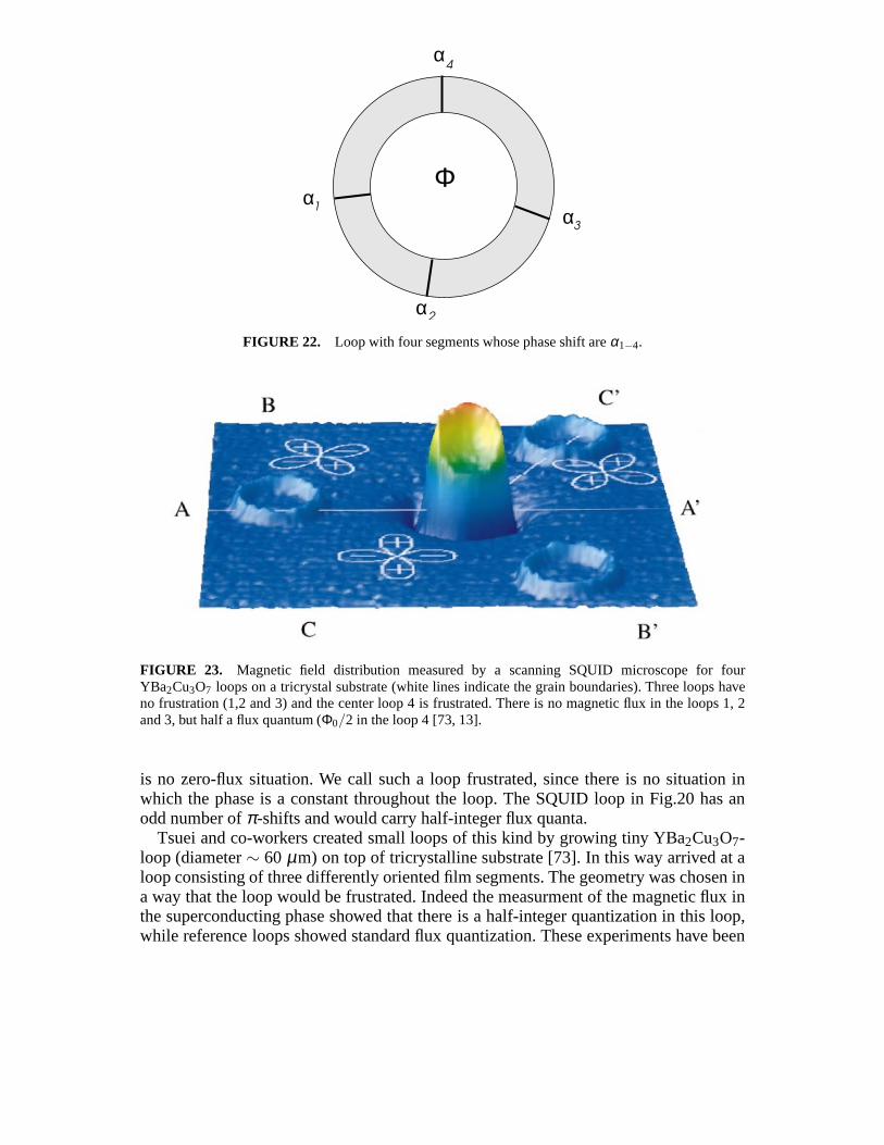
α4

αΦ

1

α2

α3

FIGURE 22. Loop with four segments whose phase shift areα1−4.

3

1

2

4

FIGURE 23. Magnetic field distribution measured by a scanning SQUID microscope for fourYBa2Cu3O7 loops on a tricrystal substrate (white lines indicate the grain boundaries). Three loops haveno frustration (1,2 and 3) and the center loop 4 is frustrated. There is no magnetic flux in the loops 1, 2and 3, but half a flux quantum (Φ0/2 in the loop 4 [73, 13].

is no zero-flux situation. We call such a loop frustrated, since there is no situation inwhich the phase is a constant throughout the loop. The SQUID loop in Fig.20 has anodd number ofπ-shifts and would carry half-integer flux quanta.

Tsuei and co-workers created small loops of this kind by growing tiny YBa2Cu3O7-loop (diameter∼ 60 µm) on top of tricrystalline substrate [73]. In this way arrived at aloop consisting of three differently oriented film segments. The geometry was chosen ina way that the loop would be frustrated. Indeed the measurment of the magnetic flux inthe superconducting phase showed that there is a half-integer quantization in this loop,while reference loops showed standard flux quantization. These experiments have been

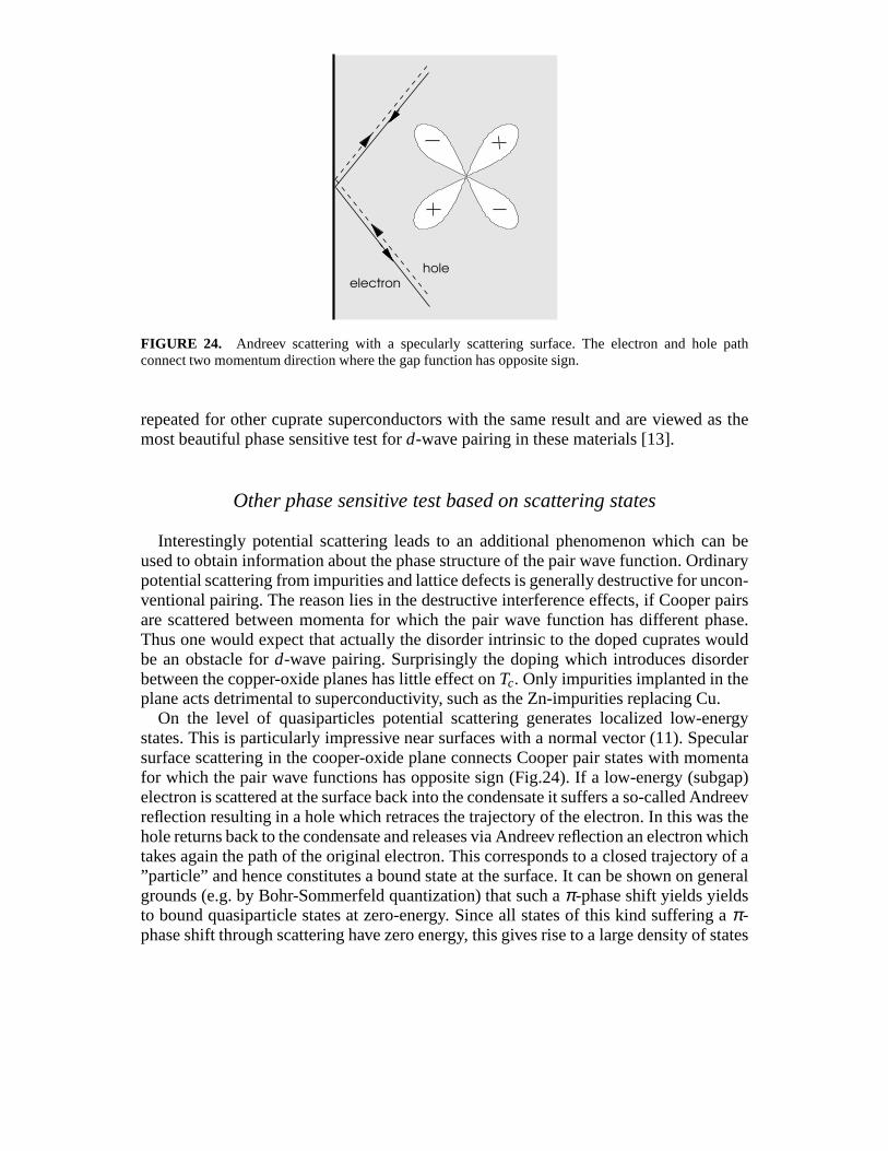
electronhole

FIGURE 24. Andreev scattering with a specularly scattering surface. The electron and hole pathconnect two momentum direction where the gap function has opposite sign.

repeated for other cuprate superconductors with the same result and are viewed as themost beautiful phase sensitive test ford-wave pairing in these materials [13].

Other phase sensitive test based on scattering states

Interestingly potential scattering leads to an additionalphenomenon which can beused to obtain information about the phase structure of the pair wave function. Ordinarypotential scattering from impurities and lattice defects is generally destructive for uncon-ventional pairing. The reason lies in the destructive interference effects, if Cooper pairsare scattered between momenta for which the pair wave function has different phase.Thus one would expect that actually the disorder intrinsic to the doped cuprates wouldbe an obstacle ford-wave pairing. Surprisingly the doping which introduces disorderbetween the copper-oxide planes has little effect onTc. Only impurities implanted in theplane acts detrimental to superconductivity, such as the Zn-impurities replacing Cu.

On the level of quasiparticles potential scattering generates localized low-energystates. This is particularly impressive near surfaces witha normal vector (11). Specularsurface scattering in the cooper-oxide plane connects Cooper pair states with momentafor which the pair wave functions has opposite sign (Fig.24). If a low-energy (subgap)electron is scattered at the surface back into the condensate it suffers a so-called Andreevreflection resulting in a hole which retraces the trajectoryof the electron. In this was thehole returns back to the condensate and releases via Andreevreflection an electron whichtakes again the path of the original electron. This corresponds to a closed trajectory of a”particle” and hence constitutes a bound state at the surface. It can be shown on generalgrounds (e.g. by Bohr-Sommerfeld quantization) that such aπ-phase shift yields yieldsto bound quasiparticle states at zero-energy. Since all states of this kind suffering aπ-phase shift through scattering have zero energy, this givesrise to a large density of states

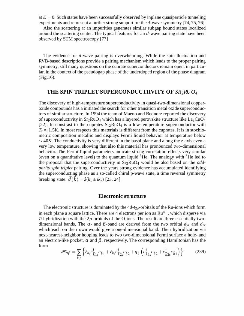
atE = 0. Such states have been successfully observed by inplane quasiparticle tunnelingexperiments and represent a further strong support for thed-wave symmetry [74, 75, 76].

Also the scattering at an impurities generates similar subgap bound states localizedaround the scattering center. The typical features for and-wave pairing state have beenobserved by STM spectroscopy [77]

The evidence ford-wave pairing is overwhelming. While the spin fluctuation andRVB-based descriptions provide a pairing mechanism which leads to the proper pairingsymmetry, still many questions on the cuprate superconductors remain open, in particu-lar, in the context of the pseudogap phase of the underdoped region of the phase diagram(Fig.16).

THE SPIN TRIPLET SUPERCONDUCTIIVITY OF SR2RUO4

The discovery of high-temperature superconductivity in quasi-two-dimensional copper-oxide compounds has a initiated the search for other transition metal oxide superconduc-tors of similar structure. In 1994 the team of Maeno and Bednorz reported the discoveryof superconductivity in Sr2RuO4 which has a layered perovskite structure like La2CuO4[22]. In constrast to the cuprates Sr2RuO4 is a low-temperature superconductor withTc ≈ 1.5K. In most respects this materials is different from the cuprates. It is in stochio-metric composition metallic and displays Fermi liquid behavior at temperature below∼ 40K. The conductivity is very different in the basal plane and along thez-axis even avery low temperature, showing that also this material has pronounced two-dimensionalbehavior. The Fermi liquid parameters indicate strong correlation effects very similar(even on a quantitative level) to the quantum liquid3He. The analogy with3He led tothe proposal that the superconductivity in Sr2RuO4 would be also based on theodd-parity spin tripletpairing. Over the years strong evidence has accumulated identifyingthe superconducting phase as a so-called chiral p-wave state, a time reversal symmetrybreaking state:~d(~k) = z(kx± iky) [23, 24].

Electronic structure

The electronic structure is dominated by the 4d-t2g-orbitals of the Ru-ions which formin each plane a square lattice. There are 4 electrons per ion as Ru4+, which disperse viaπ-hybridization with the 2p-orbitals of the O-ions. The result are three essentially two-dimensional bands. Theα- and β -band are derived from the two orbitaldyz and dzxwhich each on their own would give a one-dimensional band. Their hybridization vianext-nearest-neighbor hopping leads to two two-dimensional Fermi surface a hole- andan electron-like pocket,α andβ , respectively. The corresponding Hamiltonian has theform

Hαβ = ∑~k,s

εkyc

†~k1s

c~k1 + εkxc†~k2s

c~k2+g~k

(c†~k1s

c~k2 +c†~k2s

c~k1

)(239)

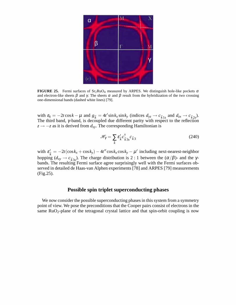
α

γ

β

FIGURE 25. Fermi surfaces of Sr2RuO4 measured by ARPES. We distinguish hole-like pocketsαand electron-like sheetsβ andγ. The sheetsα andβ result from the hybridization of the two crossingone-dimensional bands (dashed white lines) [79].

with εk = −2t cosk− µ andg~k = 4t ′sinkxsinky (indicesdyz → c~k1s anddzx → c~k2s).The third band,γ-band, is decoupled due different parity with respect to thereflectionz→−z as it is derived fromdxy. The corresponding Hamiltonian is

Hγ = ∑~k

ε ′~kc†~k3s

c~k3 (240)

with ε ′~k = −2t(coskx + cosky)− 4t ′′coskxcosky− µ ′ including next-nearest-neighborhopping (dxy → c~k3s). The charge distribution is 2 : 1 between the (α/β )- and theγ-bands. The resulting Fermi surface agree surprisingly wellwith the Fermi surfaces ob-served in detailed de Haas-van Alphen experiments [78] and ARPES [79] measurements(Fig.25).

Possible spin triplet superconducting phases

We now consider the possible superconducting phases in thissystem from a symmetrypoint of view. We pose the preconditions that the Cooper pairs consist of electrons in thesame RuO2-plane of the tetragonal crystal lattice and that spin-orbit coupling is now

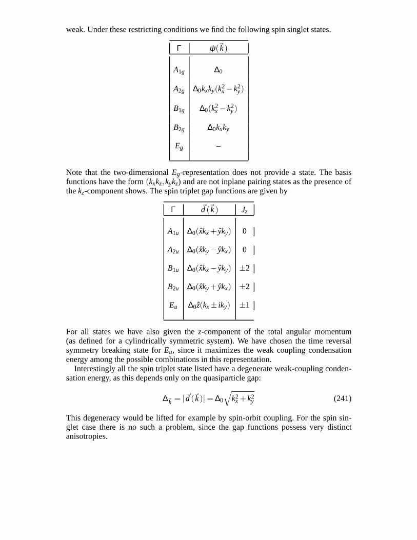
weak. Under these restricting conditions we find the following spin singlet states.

Γ ψ(~k)

A1g ∆0

A2g ∆0kxky(k2x −k2

y)

B1g ∆0(k2x −k2

y)

B2g ∆0kxky

Eg –

Note that the two-dimensionalEg-representation does not provide a state. The basisfunctions have the form(kxkz,kykz) and are not inplane pairing states as the presence ofthekz-component shows. The spin triplet gap functions are given by

Γ ~d(~k) Jz

A1u ∆0(xkx + yky) 0

A2u ∆0(xky− ykx) 0

B1u ∆0(xkx− yky) ±2

B2u ∆0(xky + ykx) ±2

Eu ∆0z(kx± iky) ±1

For all states we have also given thez-component of the total angular momentum(as defined for a cylindrically symmetric system). We have chosen the time reversalsymmetry breaking state forEu, since it maximizes the weak coupling condensationenergy among the possible combinations in this representation.

Interestingly all the spin triplet state listed have a degenerate weak-coupling conden-sation energy, as this depends only on the quasiparticle gap:

∆~k = | ~d(~k)| = ∆0

√k2

x +k2y (241)

This degeneracy would be lifted for example by spin-orbit coupling. For the spin sin-glet case there is no such a problem, since the gap functions possess very distinctanisotropies.

Experimental identification of pairing symmetry

As mentioned earlier there is convincing evidence for spin triplet pairing with thesymmetry ~d(~k) = z(kx ± iky). A first proof for unconventional superconductivity isprovided by the sensitivity of theTc to non-magnetic impurities [80]. The transitiontemperature is suppressed with increasing impurity concentration. The threshold meanfree path of the conduction electrons needs to be longer thanroughly 100 nm whichcorresponds approximately to the zero-temperature coherence length.

A rather direct test for triplet pairing is the measurement of the spin susceptibilitywhich is possible in the superconducting phase via the NMR Knight shift. Early onexperiments showed that the spin susceptibility stays constant for magnetic fields inthe basal plane indicating a~d -vector parallel to thez-axis [81]. In another experiment,the muon zero-field relaxation rate displays an pronounced continuous increase of theintrinsic magnetic field spread pointing towards a time reversal symmetry breakingsuperconducting phase [44]. From our classification we see that under the restriction toinplane pairing there is no spin singlet pairing phase with broken time reversal symmetry.On the other hand, both experiments are consistent with eachother in selecting~d(~k) =z(kx± iky).

There is further experimental evidence for this pairing state. Very recently a first phasesensitive test of the SQUID-type has been reported [82]. In contrast to the case discussedfor thedx2−y2-wave spin singlet superconductor, the conditions here is less intuitive. Afirst problem which has to be settled is the Josephson effect between a spin singlet anda spin triplet superconductor, since the SQUID device contains junctions between thetriplet and a conventional superconductor. There are two obstacles to be overcome. Thepair wave functions in the two superconductors do not match in the parity of their orbitalpart and also not in the spin part. The first point is solved through the fact that an interfacenaturally breaks parity. The second requires magneticallyactive tunneling, i.e. spin flipprocesses in tunneling. This appears automatically when the two superconductors aredifferent in spin-orbit coupling, so that the matching of electron spinor wavefunctionsremoves spin conservation in tunneling. Symmetry considerations lead to the followingexpression for the coupling:

J ∝ Im〈ψ(~k)∗ ~d(~k) · ~n×~k〉~k,FS (242)

where~n is the normal vector of the interface on the spin triplet superconductor side.We see that there is only coupling in the basal plane for~d ‖ z. The orbital and spinpart have no independent selection rules anymore, but only the total angular momentum~J · ~n perpendicular to the junction. For the gap function~d(~k) = z(ηxkx + ηyky) withthe normal vector~n ‖ x we find the thes-wave order parameter couples to theηy

component. In this way~J · ~n = 0 is realized for the Cooper pairs on both sides. TheSQUID device follow the basic design proposed by Geshkenbein and co-workers [68]as shown in Fig.26. Thes-wave superconductor is attached on two opposite sides sothat~n has opposite sign. In this way there is a phase shift ofπ in the SQUID loop and,analogously to thed-wave SQUID of the cuprate superconductors, we expect a shift ofthe interference pattern by half of a flux quantum. This effect has indeed been observed

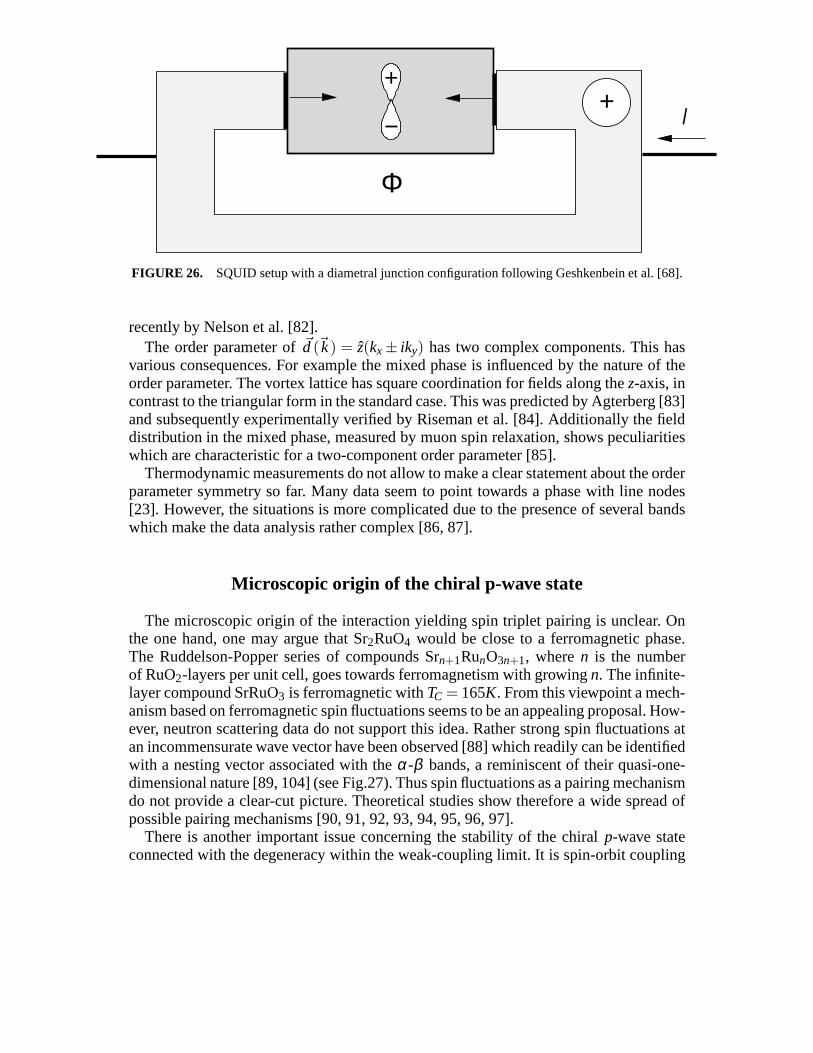
I

Φ

++

FIGURE 26. SQUID setup with a diametral junction configuration following Geshkenbein et al. [68].

recently by Nelson et al. [82].The order parameter of~d(~k) = z(kx± iky) has two complex components. This has

various consequences. For example the mixed phase is influenced by the nature of theorder parameter. The vortex lattice has square coordination for fields along thez-axis, incontrast to the triangular form in the standard case. This was predicted by Agterberg [83]and subsequently experimentally verified by Riseman et al. [84]. Additionally the fielddistribution in the mixed phase, measured by muon spin relaxation, shows peculiaritieswhich are characteristic for a two-component order parameter [85].

Thermodynamic measurements do not allow to make a clear statement about the orderparameter symmetry so far. Many data seem to point towards a phase with line nodes[23]. However, the situations is more complicated due to thepresence of several bandswhich make the data analysis rather complex [86, 87].

Microscopic origin of the chiral p-wave state

The microscopic origin of the interaction yielding spin triplet pairing is unclear. Onthe one hand, one may argue that Sr2RuO4 would be close to a ferromagnetic phase.The Ruddelson-Popper series of compounds Srn+1RunO3n+1, wheren is the numberof RuO2-layers per unit cell, goes towards ferromagnetism with growing n. The infinite-layer compound SrRuO3 is ferromagnetic withTC = 165K. From this viewpoint a mech-anism based on ferromagnetic spin fluctuations seems to be anappealing proposal. How-ever, neutron scattering data do not support this idea. Rather strong spin fluctuations atan incommensurate wave vector have been observed [88] whichreadily can be identifiedwith a nesting vector associated with theα-β bands, a reminiscent of their quasi-one-dimensional nature [89, 104] (see Fig.27). Thus spin fluctuations as a pairing mechanismdo not provide a clear-cut picture. Theoretical studies show therefore a wide spread ofpossible pairing mechanisms [90, 91, 92, 93, 94, 95, 96, 97].

There is another important issue concerning the stability of the chiral p-wave stateconnected with the degeneracy within the weak-coupling limit. It is spin-orbit coupling

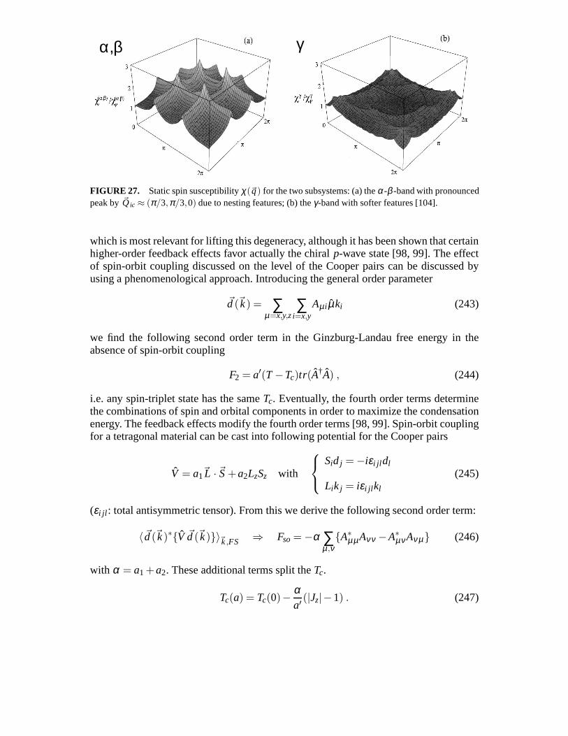
α,β γ

FIGURE 27. Static spin susceptibilityχ(~q) for the two subsystems: (a) theα-β -band with pronouncedpeak by~Q ic ≈ (π/3,π/3,0) due to nesting features; (b) theγ-band with softer features [104].

which is most relevant for lifting this degeneracy, although it has been shown that certainhigher-order feedback effects favor actually the chiralp-wave state [98, 99]. The effectof spin-orbit coupling discussed on the level of the Cooper pairs can be discussed byusing a phenomenological approach. Introducing the general order parameter

~d(~k) = ∑µ=x,y,z

∑i=x,y

Aµ i µki (243)

we find the following second order term in the Ginzburg-Landau free energy in theabsence of spin-orbit coupling

F2 = a′(T −Tc)tr(A†A) , (244)

i.e. any spin-triplet state has the sameTc. Eventually, the fourth order terms determinethe combinations of spin and orbital components in order to maximize the condensationenergy. The feedback effects modify the fourth order terms [98, 99]. Spin-orbit couplingfor a tetragonal material can be cast into following potential for the Cooper pairs

V = a1~L · ~S+a2LzSz with

Sid j = −iεi jl dl

Lik j = iεi jl kl

(245)

(εi jl : total antisymmetric tensor). From this we derive the following second order term:

〈 ~d(~k)∗V ~d(~k)〉~k,FS ⇒ Fso= −α ∑µ,ν

A∗µµAνν −A∗

µνAνµ (246)

with α = a1 +a2. These additional terms split theTc.

Tc(a) = Tc(0)− αa′

(|Jz|−1) . (247)

TheTc depends on the total angular momentumJz and onα. The sign ofα determineswhether the states withJz = ±2 or Jz = 0 have the highestTc. Annoyingly the chiralp-wave state cannot be stabilized in this way [100, 95, 101, 96]

On the microscopic level we can introduce spin-orbit coupling on the Ru-ion actingonly within the 4d-t2g-orbitals:

Hso = iλ ∑m,n,l

εlmn ∑~k,s,s′

c†~k ls

c~kms′σnss′ . (248)

This added to the tight-binding Hamiltonian (239,240) leads to a modified band struc-ture. Examining this Hamiltonian we find that starting out from the independent orbitals(dyz,dzx,dxy) we can obtain in lowest order perturbation in the spin-orbit coupling andthe interorbital hybridization that the degeneracy is lifted by a spin dependent Cooperpair scattering between the orbitalsdyz anddzx with the matrix element proportional to

λ t ′〈kxkyz· ~d1(~k)× ~d2(~k)〉~k (249)

where ~d1 and ~d2 are the gap functions associated with the orbitaldyz anddzx, respec-tively. Obviously the~d -vectors have to lie in thex-y-plane in order to reach a finitematrix element. It is easy to verify that the possible statesstabilized are characterized byJz= 0 or±2 depending on the sign ofλ . This is in agreement with the phenomenologicalanalysis above [101].

In order to stabilize the chiralp-wave state an additional indirect spin anisotropy hasto enter via the pairing interaction [102, 104, 95, 101]. This means that interactionsinvolving spin densities have to play a certain role in the pairing mechanism in orderto pin the orientation of the~d -vector additionally. The spin fluctuation mechanism, forexample, involves the anisotropies of the dynamical spin susceptibility resulting fromspin-orbit coupling in the multi-band systems (248). The static susceptibility shows veryclear properties in this respect:

χzz(~q) < χ+−(~q) for ~q → 0

χzz(~q) < χ+−(~q) for ~q = ~Q ic

(250)

where ~Q ic ≈ (π/3,π/3,0) is the wave vector of the (dominant) incommensurate spincorrelation [104, 105]. The small-q contribution is inplane polarized and the incom-mensurate fluctuations arez-axis polarized [106]. The former favors, of course, inplaneequal-spin pairing for the spin triplet channel, since the small-q scattering is favorablefor odd-parity pairing[102]. Thez-axis polarization on the other hand, is essential forcertain spin fluctuation based mechanisms combining the scattering around~Q ic andspecial nesting feartures of the Fermi surface to obtained an inplane equal-spin pairingstate [91, 93]. While this aspect suggests that spin fluctuations are involved in the pairingmechanism, it is not clear whether they are necessarily the dominant part. In addition theview on the spin dynamics alone neglects contributions fromvertex corrections (renor-malized coupling matrx elements) which are possibily important for the selection of thepairing state as well [90, 95].

We have two competing trends due to spin-orbit coupling. If the α-β -bands aredominating the superconductivity, then likely the states with ~d ⊥ zwill be stabilized. Onthe other hand, a dominatingγ-band would entirely be determined by the contributionsof the anisotropic spin fluctuations stabilizing a state with ~d ‖ z corresponding to thechiral p-wave phase. Therefore, aγ-band dominating the superconducting instabilitywhile the α-β -bands are only passively involved, provides good conditions to favorthe chiral p-wave state over the others [103, 95]. This ideas of the dominant γ-bandreceives strong support from the analysis of various thermodynamic measurements suchas the specific heat [87, 107], the London penetration depth [108, 109] etc. These resultssuggest that theα-β -bands only contribute at rather low temperature noticablyto thesuperconductivity. This aspect makes the search for gap anisotropies, even with nodalfeatures, very challenging [107].

The fact that there are obviously two trends to lift the degeneracy among the differentspin triplet states hints that the energy scales involved inthe end are rather small despitethe rather strong spin orbit coupling (λ ∼ 1000K). There are several renormalizingsteps which reduce finally the magnitude of effect on the Cooper pair energy. Forexample the matrix element (249) is reduced through the factthat contributions to the~k average come from the region at the Fermi level where the two bands cross. Also thecontribution of the anisotropy of the spin susceptibility can only result in a fraction ofTc. Consequently the anisotropy pinning of the~d -vector is likely weak. Indeed recentKnight shift measurement for fields along thez-axis suggest that for fields of severalhundreds of Oe the~d may have flipped into basal plane [110].

The inhomogeneous 3-Kelvin phase

Finally we would like to briefly review a quite unexpected finding in Sr2RuO4. Inves-tigating Ru-Sr2RuO4 eutectic samples it was found that an inhomogeneous supercon-ducting phase appears at higher temperature than the bulk superconductivity, roughlyaroundT∗ ∼ 3K. This inhomogeneous phase was then called ”3K-phase”. Below T∗

superconductivity nucleates on islands which eventually grow together to form the uni-form bulk phase as the temperature reachesTc ≈ 1.5K. The signature of the phase is thegradual drop of the resistance forTc < T < T∗[111]. The Ru-Sr2RuO4 eutectic consistsof manyµm-size Ru-metal inclusions in the otherwise pure Sr2RuO4. The experimentalevidence points towards the nucleation of superconductivity at the interface between Ruand Sr2RuO4 in a way that in a tiny layer the conditions for Cooper pairingis improved[112]. The nucleation of such a filamentary form of superconductivity has been con-firmed by measurments of the upper critical field. For filamentary superconductors thetemperature dependence of the upper critical field has an exponentα < 1 in

Hc2(T) ∝ (T∗−T)α (251)

whereα has been fitted to the value 0.7. This means a clear deviation from the standardbulk Hc2 which has a linear dependence [113, 114].

A fascinating aspect of this eutectic system is that the nucleated order parameter hasa p-wave component whose lobes lie parallel to the interface. This corresponds to time

reversal symmetry conserving phase, so that the bulk transition is not merely a perco-lation transition as in inhomogeneous conventional superconductors. This transition istime reversal symmetry breaking in order to arrive at the chiral p-wave phase. The studyof the structure of the inhomogeneous phase shows that the transition to the bulk phasemay be even more complex. The inhomogeneous phase viewed as anetwork of super-conducting islands weakly coupled among each other, which is intrinsically frustrateddue to the internal phase structure. Thus, the evolution of the superconducting phase asthe temperature is lowered could lead through regimes wherespontaneous supercurrentsare flowing in the frustrated network, rather similar to the frustrated loops discussed inthe context of phase sensitive test ford-wave superconductivity [112]. For such a phasethere is so far only indirect evidence by the observation that the critical currents in the3-K phase are not invariant under the operationJ → −J [115]. This indicates that inthe complex network of superconducting islands the time reversal symmetry has beenbroken.

It is a lucky coincidence that Sr2RuO4 provides us with this highly complex inhomo-geneous phase besides much other exciting physics of an unconventional superconduc-tor. While a great deal of the properties of this superconductor has been understood bynow there are still many questions. In particular, the pairing mechanism and its connec-tion to the magnetic properties have not been put into a transparent form. Sr2RuO4 willin any case serve in future as an exemplary system for discussing unconventional su-perconductivity as many of the generic non-trivial aspectsare realized here. As a Fermiliquid phase it constitutes also the electronic analog of the most intriguing superfluid,3He.

CONCLUSION

In this lecture we have covered a few of the essential parts todescribe and understandunconventional superconductivity. This field is quickly developing due to impressiveprogress in the production of high-quality materials during recent years. High qualityis mandatory to find unconventional superconductivity, since anisotropic Cooper pairsare easily destroyed by scattering at defects in the samples. Among the unconventionalsuperconductors we do not only find those with the highestTc but many with fascinatingand puzzling properties making them despite most lowTcs a most attractive subject ofresearch. Many of the new superconductors require from us toextend our views andideas of superconductivity.

Finally I would like to recommend for further reading several reviews and bookswhich go in many parts much deeper than it was possible in thislecture. Among thebooks to recommend are V.P. Mineev and K.V. Samokhin,Introduction to Unconven-tional Superconductivity(Gordon and Breach, Science Publisher, 1999), K.H. Benne-mann and J.B. Ketterson,The Physics of Superconductors, Vol. I / II(Springer, 2003).A review on recent developments for the heavy Fermion superconductor UPt3, not men-tioned in the lecture, is R. Joynt and L. Taillefer (Rev. Mod.Phys. 74, 235 (2002)).

ACKNOWLEDGMENTS

I would like to thank my colleagues with whom I had the pleasure to work on thesubjects which have been topics of this lecture: D.F. Agterberg, Y. Asano, P.A. Frigeri,A. Furusaki, J. Goryo, N. Hayashi, C. Honerkamp, H. Kusunose, M. Matsumoto, H.Monien, K.K. Ng, Y. Okuno, Y. Tanaka, F.C. Zhang, M.E. Zhitomirsky. In particular Iwould like to thank T.M. Rice, K. Ueda and R. Joynt who introduced me to the fieldmany years ago, and my experimental colleagues Y. Maeno, A.P. Mackenzie, A.C. Motaand H.R. Ott. I would also like to thank Guillaume Roux who helped the preparation ofthis notes in the initial stage.

REFERENCES

1. P. W. Anderson and P. Morel, Phys. Rev. Lett.5, 136-138 (1960); Phys. Rev.123, 1911-1934 (1961).2. R. Balian and N. R. Werthamer, Phys. Rev.131, 1553-1564 (1963).3. A. J. Leggett, Rev. Mod. Phys.47, 331-414 (1975).4. D. D. Osheroff, R. C. Richardson and D. M. Lee, Phys. Rev. Lett. 28, 885-887 (1972).5. D. Vollhardt and P. Wölfle,The superfluid phases of3He, Tayler & Francis, London (1990).6. F. Steglich, J. Aarts, C.D. Bredl, W. Lieke, D. Meschede, W. Franz and H. Schäfer, Phys. Rev. Lett.

43, 1892 (1979).7. H.R. Ott, H. Rudigier, Z. Fisk and J.L. Smith, Phys. Rev. Lett. 50, 1595 (1983).8. G.R. Stewart, Z. Fisk, J.O. Willis and J.L. Smith, Phys. Rev. Lett.52, 679 (1984).9. D. Jerome, A. Mazaud, M. Ribault and K. Bechgaard, J. Phys.Lett. (Paris)41, L95 (1980).10. S.S.P. Parkin, E.M. Engler, R.R. Schumaker, R. Lagier, V.V. Lee, J.C. Scott and R.L. Greene, Phys.

Rev. Lett.50, 270 (1983).11. J.G. Bednorz and K.A. Müller, Z. Phys. B64, 189 (1986).12. D.J. Scalapino, Phys. Rep.250, 329 (1995).13. C.C. Tsuei and J.R. Kirtley, Rev. Mod. Phys.72, 969 (2000).14. B. Batlogg and C. Varma, Physics World, Feb. 2000, p. 33.

(http://physicsweb.org/article/world/13/2/8)15. F.M. Grosche, S.R. Julien, N.D. Mathurand G.G. Lonzarich, Physica B223-224, 50 (1996).16. N.D. Mathur, G.M. Grosche, S.R. Julian, I.R. Walker, D.M. Freye, R.K.W. Haselwimmer, G.G.

Lonzarich, Nature (London)394, 39 (1998).17. J.D. Thompson, R. Movshovich, Z. Fisk, F. Bouquet, N.J. Cueeo, R.A. Fisher, P.C. Hammel, H.

Heeger, M.F. Hundley, M. Jaime, P.G. Pagliuso, C. Petrovic,N.E. Philips, J.L. Sarrao, J. Magn. Magn.Mater.226-230, 5 (2001).

18. C. Petrovic, R. Movshovich, M. Jaime, P.G. Hundley, J.L.Sarrao, Z. Fisk, J.D. Thompson, Europhys.Lett. 53, 354 (2001).

19. S.S. Saxena, P. Agarwal, K. Ahllan, F.M. Grosche, R.K.W.Haselwimmer, M.J. Steiner, E. Pugh,I.R. Walker, S.R. Julian, P. Monthoux, G.G. Lonzarich, A. Huxley, I. Shelkin, D. Braithwaite, and J.Flouquet, Nature (London)406, 587 (2000).

20. D. Aoki, A. Huxley, E. Ressouche, D. Braithwaite, J. Flouquet, J.-P. Brison, and E. Lhotel, Nature413, 613 (2001).

21. C. Pfleiderer, J. Magn. Magn. Mater,226-230, 23 (2001).22. Y. Maeno, H. Hashimoto, K. Yoshida, S. Nishizaki, T. Fujita, J.G. Bednorz and F. Lichtenberg, Nature

(London)372, 532 (1994).23. A.P. Mackenzie and Y. Maeno, Rev. Mod. Phys.75, 657 (2003).24. Y. Maeno, T.M. Rice and M. Sigrist, Physics Today54, 42 (2001).25. E.D. Bauer, N.A. Frederick, P.-C. Ho, V.S. Zapf, and M.B.Maple, Phys. Rev. B65, 100506 (R)

(2002).26. K. Takada, H. Sakurai, E. Takayama-Muromachi, F. Isumi,R.A. Dilanian and T. Sasaki, Nature

(London)422, 53 (2003).

27. M. Hanawa, Y. Muraoka, T. Tayama, T. Sakakibara, J. Yamaura and Z. Hiroi, Phys. Rev. Lett.87,187001 (2001).

28. S. Yonezawa, Y. Muraoka, Y. Matsushita and Z. Hiroi, J. Phys. Cond. Matter16 , L9 (2004).29. E. Bauer, G. Hilscher, H. Michor, C. Paul, E.W. Scheidt, A. Gribanov, Y. Seropegin, H. Noel, M.

Sigrist and P. Rogl, Phys. Rev. Lett.92, 027003 (2004).30. P. W. Anderson and P. Morel, Phys. Rev.125, 1263-1271 (1962).31. W. L. MacMillan, Phys. Rev.167, 331 (1968).32. W. Kohn and J.M. Luttinger, Phys. Rev. Lett.15, 524-526 (1965).33. N.F. Berk and J.R. Schrieffer, Phys. Rev. Lett.17, 433-435 (1966).34. D. Fay and J. Appel, Phys. Rev. B22, 3173-3182 (1980).35. P. Monthoux and G.G. Lonzarich, Phys. Rev. B59, 14598 (1999); Phys. Rev. B63, 054529 (2001).36. T. Akazawa, H. Hidaka, T. Fujiwara, T.C. Kobayashi, E. Yamamoto, Y. Haga, R. Settai and Y. Onuki,

J. Phys.: Condens. Matter16, L29 (2004); T. Akazawa, H. Hidaka, T.C. Kobayashi,T. Fujiwara E.Yamamoto, Y. Haga, R. Settai and Y. Onuki, J. Phys. Soc. Jpn.73, 3129 (2004).

37. P.W. Anderson and W.F. Brinkman, included in P.W. Anderson Basic Notions of Condensed MatterPhysics, Frontiers in Physics Nr. 55, Addison-Wesley (1984).

38. P.W. Anderson, J. Phys. Chem. Solids11, 26 (1959).39. P.W. Anderson, Phys. Rev. B30, 4000 (1984).40. P.W. Anderson and W.F. Brinkman, Phys. Rev. Lett.30, 1108 (1973).41. A.A. Abrikosov,Fundamentals of the Theory of Metals, North-Holland, Chapter: 21.4 (1988).42. L.P. Gorkov, Sov. Sci. Rev. A Phys.9, 1 (1987).43. M. Sigrist and K. Ueda, Rev. Mod. Phys.63, 239 (1991).44. G.M. Luke, Y. Fudamoto, K.M. Kojima, M.I. Larkin, J. Merrin, B. Nachumi, Y.J. Uemura, Y. Maeno,

Z.Q. Mao, Y. Mori, H. Nakamura and M. Sigrist, Nature (London) 394, 558 (1998).45. R.H. Heffner, J.O. Willis, J.L. Smith, P. Birrer, C. Baines, F.N. Gygax, B. Hitti, E. Lippelt, H.R. Ott,

A. Schenk and D.E. MacLaughlin, Phys. Rev. B40, 806 (1989).46. H.R. Ott, H. Rudigier, E. Felder, Z. Fisk and J.L. Smith, Phys. Rev. B33, 126 (1986).47. H.R. Ott, J. Low Temp. Phys.95, 95 (1994).48. G.M. Luke, A. Keren, L.P. Le, W.D. Wu, Y.J. Uemura, D.A Bonn, L. Taillefer and J.D. Garrett, Phys.

Rev. Lett.71, 1466 (1993).49. R.A. Fisher, S. Kim, B.F. Woodfield, N.E. Phillips, L. Taillefer, K. Hasselbach, J. Flouquet, A.L.

Giorgi and J.L. Smith, Phys. Rev. Lett.62, 1411 (1989).50. K. Hasselbach, L. Taillefer and J. Flouquet, Phys. Rev. Lett.63, 93 (1989).51. Y. Aoki, A. Tsuchiya, T. Kanayama, S.R. Saha, H. Sugawara, H. Sato, W. Higemoto, A. Koda, K.

Ohishi, K.Nishiyama and R. Kadono, Phys. Rev. Lett.91, 067003 (2003).52. F.C. Zhang and T.M. Rice, Phys. Rev. B37, 3759 (1988).53. T. Moriya,Spin fluctuations in itinerant electron magnetism, Springer Series in Solid-State Sciences

56 (1985).54. P.W. Anderson, Science237, 1196 (1987).55. P.W. Anderson, P.A. Lee, M. Randeria, T.M. Rice, N. Trivedi and F.C. Zhang, J. Phys. Condens.

Matter16, R755 (2004).56. P.A. Lee, N. Nagaosa and X.G. Wen, cond-mat/0410445.57. N. Nagaosa,Quantum Field Theory in Strongly Correlated Electronic Systems, Springer (1998).58. T. Moriya and K. Ueda, Adv. Phys. 49, 555 (2000).59. T. Tanamoto, H Kohno and H. Fukuyama, J. Phys. Soc. Jpn. 63, 2739 (1994).60. J.A. Martindale, S.E. Barrett, K.E. O’Harea, C.P. Slichter, W.C. Lee and D.M. Ginsberg, Phys. Rev.

B 47, 9155 (1993).61. W.N. Hardy, D.A. Bonn, D.C. Morgan, R. Liang and K. Zhang,Phys. Rev. Lett.70, 3999 (1993).62. B. Barbiellini, O. Fischer, M. Peter, C. Renner and M. Weger, Physica C220, 55.63. Z.X. Shen, D.S. Dessau, B.O. Wells, D.M. King, W.E. Spicer, A.J. Arko, D. Marshall, L.W. Lom-

bardo, A. Kapitulnik, P. Dickinson, S. Doniach, J. DiCarlo,A.G. Loeser and C.H. Park, Phys. Rev.Lett. 70, 1553 (1993).

64. H. Ding, M.R. Norman, J.C. Campuzano, M. Randeria, A.F. Bellman, T. Yokoya, T. Takahashi, T.Mochiku and K. Kadowaki, Phys. Rev. Lett.54, 9678 (1996).

65. A. Damascelli, Z. Hussain and Z.X. Shen. Rev. Mod. Phys.75, 473 (2003).66. D.J. Van Harlingen, Rev. Mod. Phys.67, 515 (1995).

67. V.B. Geshkenbein and A.I. Larkin, JETP Lett.43, 395 (1986).68. V.B. Geshkenbein, A.I. Larkin and A. Barone, Phys. Rev. B36, 235 (1987).69. M. Sigrist and T.M. Rice, J. Phys. Soc. Jpn.61, 4283 (1992).70. D.A. Wollman, D.J. Van Harlingen, W.C. lee, D.M. Ginsberg and A.J. Leggett, Phys. Rev. Lett.71,

2134 (1993).71. D. Brawner and H.R. Ott, Phys. Rev. B50, 6530 (1994).72. A. Mathai, Y. Gim, R.C. Black, A. Amar and F.C. Wellstood,Phys. Rev. Lett.74, 4523 (1995).73. C.C. Tsuei, J.R. Kirtley, C.C. Chi, L.S. Yu-Jahnes, A. Gupta, T. Shaw, J.Z. Sun and M.B. Ketchen,

Phys. Rev. Lett.73, 593 (1994).74. C.-R. Hu, Phys. Rev. Lett.72, 1526 (1994).75. S. Kashiwaya and Y. Tanaka, Rep. Prog. Phys.63, 1641 (2000).76. G. Deutscher, Rev. Mod. Phys.77, 109 (2005).77. A.V. Balatsky, I. Vekhter and J.-X. Zhu, cond-mat/0411318 (2004).78. C. Bergemann, S.R. Julian, A.P. Mackenzie, S. Nishizakiand Y. Maeno, Phys. Rev. Lett.84, 2662

(2000).79. A. Damascelli, D.H. Lu, K.M. Shen, N.P. Armitage, F. Ronning, D.L. Feng, C. Kim, Z.X. Shen, T.

Kimura, Y. Tokura, Z.Q. Mao and Y. Maeno, Phys. Rev. Lett.85, 5194 (2000).80. A.P. Mackenzie, R.K.W. Haselwimmer, A.W. Tyler, G.G. Lonzarich, Y. Mori, S. Nishizaki and Y.

Maeno, Phys. Rev. Lett.80, 161 (1998).81. K. Ishida, H. Mukuda, Y. Kitaoka, K. Asayama, Z.Q. mao, Y.Mori and Y. Maeno, Nature (London)

396, 658 (1998).82. K.D. Nelson, Z.Q. Mao, Y. Maeno and Y. Liu, Science306, 1151 (2004).83. D.F. Agterberg, Phys. Rev. Lett.80, 5184 (1998).84. T.M. Riseman, P.G. Kealey, E.M. Forgan, A.P. Mackenzie,L.M. Galvin, A.W. Tyler, S.L. Lee, C.

Ager, D. McK. Paul, C.M. Aegerter, R. Cubitt, Z.Q. Mao, T. Akima and Y. Maeno, Nature (London)396, 242; Nature (London)404, 629 (2000).

85. P.G. Kealey, T.M. Riseman, E.M. Forgan, A.P. Mackenzie,L.M. Galvin, S.L. Lee, D.McK. Paul, R.Cubitt, D.F. Agterberg, R. Heeb, Z.Q. Mao and Y. Mao, Phys. Rev. Lett.84, 6094 (2000).

86. D.F. Agterberg, T.M. Rice and M. Sigrist, Phys. Rev. Lett. 78, 3374 (1997).87. M.E. Zhitomirsky and T.M. Rice, Phys. Rev. Lett.87, 057001 (2001).88. Y. Sidis, M. Braden, P. Bourges, B. Hennion, W. Reichardt, Y. Maeno and Y. Mori, Phys. Rev. Lett.

83, 3320 (1999).89. I.I. Mazin and D.J. Singh, Phys. Rev. Lett.82, 4324 (1999).90. T. Nomura and K. Yamada, J. Phys. Soc. Jpn.69, 2678 (2000); J. Phys. Soc. Jpn.71, 404 (2002);J.

Phys. Soc. Jpn.71, 1993 (2002).91. T. Kuwabara and M. Ogata, Phys. Rev. Lett.85, 4586 (2000).92. M. Sato and K. Kohmoto, J. Phys. Soc. Jpn.69, 3505 (2000).93. K. Kuroki, M. Ogata, R. Arita and H. Aoki, Phys. Rev. B63, 060506 (2001).94. I. Eremin, D. Manske, C. Joas and K.H. Bennemann, Europhys. Lett.58, 871 (2002).95. Y. Yanase and M. Ogata, J. Phys. Soc. Jpn.72, 673 (2003).96. I. Eremin, D. Manske, S.G. Ovchinnikov and J.F. Annett, Annalen der Physik13, 149 (2004).97. R. Arita, S. Onari, K. Kuroki and H. Aoki, Phys. Rev. Lett.bf 92, 247006 (2004).98. J. Goryo and M. Sigrist, J. Phys.: Condens. Matter12, L599 (2000).99. J. Goryo and M. Sigrist, Europhys. Lett.57, 578 (2002).100. M. Sigrist and M.E. Zhitomirsky, J. Phys. Soc. Jpn.65, 3452 (1996).101. J.F. Annett, G. Litak, B.L. Gyorffy and K.L. Wysokinski, cond-mat/0411169.102. M. Sigrist, D.F. Agterberg, A. Furusaki, C. Honerkamp,K.K. Ng, T.M. Rice and M.E. Zhitomirsky,

Physica C317-318, 134 (1999).103. K.K. Ng and M. Sigrist, Europhys. Lett.49, 473 (2000).104. K.K. Ng and M. Sigrist, J. Phys. Soc. Jpn.69, 3764 (2000).105. I. Eremin, D. Manske and K.H. Bennemann, Phys. Rev. B65, 220502 (2002).106. M. Braden, P. Steffens, Y. Sidis, J. Kulda, P. Bourges, S. Hayden, N. Kikugawa and Y. Maeno, Phys.

Rev. Lett.92, 097402 (2004).107. K. Deguchi, Z.Q. Mao, H. Yaguchi and Y. Maeno, Phys. Rev.Lett. 92, 047002 (2004); K. Deguchi,

Z.Q. Mao and Y. Maeno, J. Phys. Soc. Jpn.73, 1313 (2004).

108. I. Bonalde, B.D. Yanoff, D.J. Van Harlingen, M.B. Salamon and Y. Maeno, Phys. Rev. Lett.85, 4775(2000).

109. H. Kusunose and M. Sigrist, Europhys. Lett.60, 281 (2002).110. H. Murakawa, K. Ishida, K. Kitagawa, Z.Q. Mao and Y. Maeno, Phys. Rev. Lett.93, 167004 (2004).111. Y. Maeno, T. Ando, Y. Mori, E. Ohmichi, S. Ikeda, S. Nishizaki and S. Nakatsuji, Phys. Rev. Lett.

81, 3765 (1998).112. M. Sigrist and H. Monien, J. Phys. Soc. Jpn.70, 2409 (2001).113. H. Yaguchi, M. Wada, T. Akima, Y. Maeno and T. Ishiguro, Phys. Rev. B67, 214519 (2003).114. M. Matsumoto, C. Belardinelli and M. Sigrist, J. Phys. Soc. Jpn.72, 1623 (2003).115. J. Hooper, Z.Q. Mao, K.D. Nelson, Y. Liu, M. Wada and Y. Maeno, Phys. Rev. B70, 014510 (2004).