Embed Size (px)
Citation preview

Introduction to Time Series Analysis. Lecture 12.Peter Bartlett
Last lecture:
1. Parameter estimation
2. Maximum likelihood estimator
3. Yule-Walker estimation
1

Introduction to Time Series Analysis. Lecture 12.
1. Review: Yule-Walker estimators
2. Yule-Walker example
3. Efficiency
4. Maximum likelihood estimation
5. Large-sample distribution of MLE
2

Review: Yule-Walker estimation
Method of moments: We choose parameters for which the moments are
equal to the empirical moments.
In this case, we chooseφ so thatγ(h) = γ(h) for h = 0, . . . , p.
Yule-Walker equations forφ:
Γpφ = γp,
σ2 = γ(0)− φ′γp.
These are the forecasting equations.
We can use the Durbin-Levinson algorithm.
3
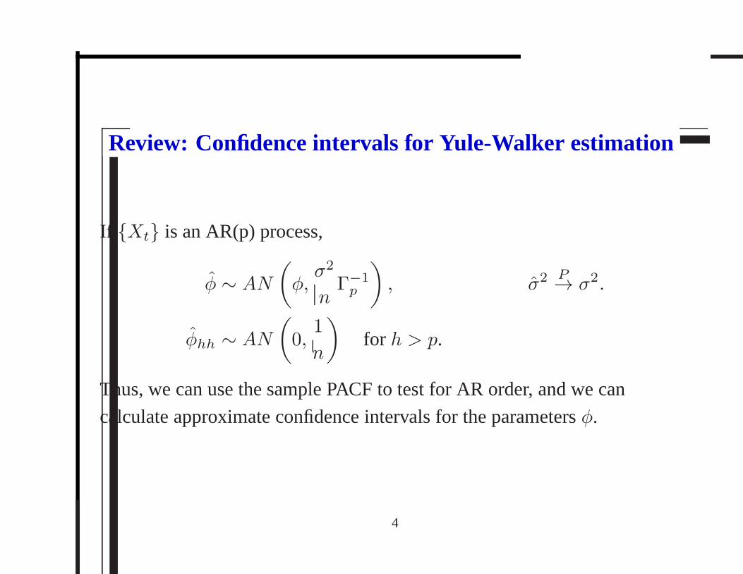
Review: Confidence intervals for Yule-Walker estimation
If {Xt} is an AR(p) process,
φ ∼ AN
(
φ,σ2
nΓ−1p
)
, σ2 P→ σ2.
φhh ∼ AN
(
0,1
n
)
for h > p.
Thus, we can use the sample PACF to test for AR order, and we can
calculate approximate confidence intervals for the parametersφ.
4
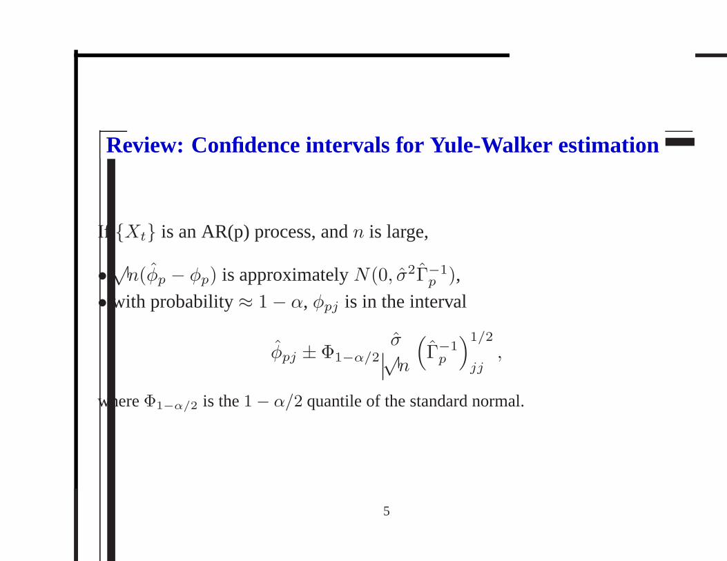
Review: Confidence intervals for Yule-Walker estimation
If {Xt} is an AR(p) process, andn is large,
• √n(φp − φp) is approximatelyN(0, σ2Γ−1p ),
• with probability≈ 1− α, φpj is in the interval
φpj ± Φ1−α/2σ√n
(
Γ−1p
)1/2
jj,
whereΦ1−α/2 is the1− α/2 quantile of the standard normal.
5

Review: Confidence intervals for Yule-Walker estimation
• with probability≈ 1− α, φp is in the ellipsoid{
φ ∈ Rp :(
φp − φ)′
Γp
(
φp − φ)
≤ σ2
nχ21−α(p)
}
,
whereχ2
1−α(p) is the(1−α) quantile of the chi-squared withp degrees of freedom.
6

Yule Walker estimation: Example
−40 −30 −20 −10 0 10 20 30 40−0.2
0
0.2
0.4
0.6
0.8
1
1.2Sample ACF: Depth of Lake Huron, 1875 − 1972
7
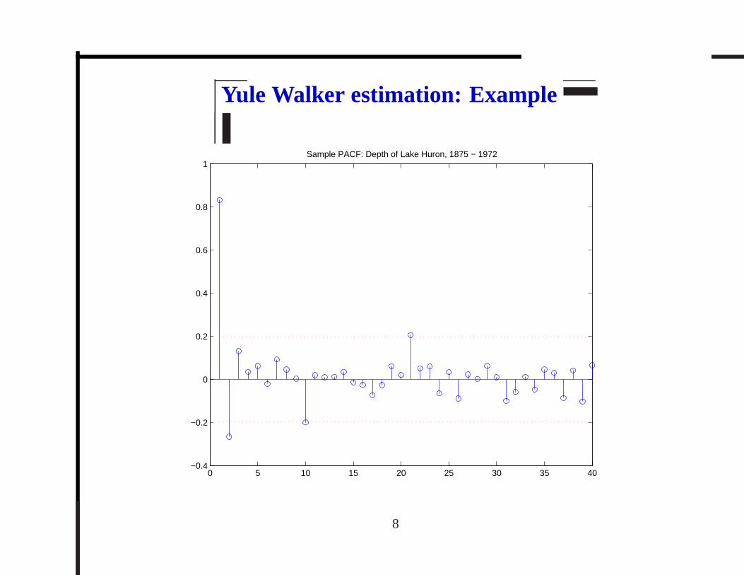
Yule Walker estimation: Example
0 5 10 15 20 25 30 35 40−0.4
−0.2
0
0.2
0.4
0.6
0.8
1Sample PACF: Depth of Lake Huron, 1875 − 1972
8
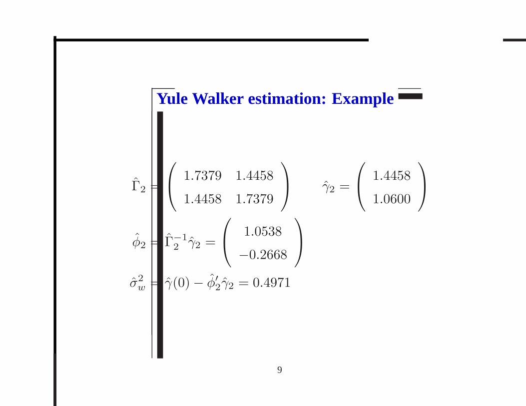
Yule Walker estimation: Example
Γ2 =
1.7379 1.4458
1.4458 1.7379
γ2 =
1.4458
1.0600
φ2 = Γ−12 γ2 =
1.0538
−0.2668
σ2w = γ(0)− φ′2γ2 = 0.4971
9

Yule Walker estimation: Example
Confidence intervals:
φ1 ± Φ1−α/2
(
σ2wΓ
−12 /n
)1/2
11= 1.0538± 0.1908
φ2 ± Φ1−α/2
(
σ2wΓ
−12 /n
)1/2
22= −0.2668± 0.1908
10

Yule-Walker estimation
It is also possible to define analogous estimators for ARMA(p,q) models
with q > 0:
γ(j)− φ1γ(j − 1)− · · · − φpγ(j − p) = σ2
q∑
i=j
θiψi−j ,
whereψ(B) = θ(B)/φ(B).
Because of the dependence on theψi, these equations are nonlinear inφi, θi.
There might be no solution, or nonunique solutions.
Also, theasymptotic efficiencyof this estimator is poor: it has unnecessarily
high variance.
11

Efficiency of estimators
Let φ(1) andφ(2) be two estimators. Suppose that
φ(1) ∼ AN(φ, σ21), φ(2) ∼ AN(φ, σ2
2).
The asymptotic efficiency ofφ(1) relative toφ(2) is
e(
φ, φ(1), φ(2))
=σ22
σ21
.
If e(
φ, φ(1), φ(2))
≤ 1 for all φ, we say thatφ(2) is amore efficient
estimator ofφ thanφ(1).
For example, for an AR(p) process, the moment estimator and themaximum likelihood estimator are as efficient as each other.
For an MA(q) process, the moment estimator is less efficient than theinnovations estimator, which is less efficient than the MLE.
12

Yule Walker estimation: Example
AR(1): γ(0) =σ2
1− φ21
φ1 ∼ AN
(
φ1,σ2
nΓ−11
)
= AN
(
φ1,1− φ21n
)
.
AR(2):
φ1
φ2
∼ AN
φ1
φ2
,σ2
nΓ−12
andσ2
nΓ−12 =
1
n
1− φ22 −φ1(1 + φ2)
−φ1(1 + φ2) 1− φ22
.
13

Yule Walker estimation: Example
Suppose{Xt} is an AR(1) process and the sample sizen is large.
If we estimateφ, we have
Var(φ1) ≈1− φ21n
.
If we fit a larger model, say an AR(2), to this AR(1) process,
Var(φ1) ≈1− φ22n
=1
n>
1− φ21n
.
We have lost efficiency.
14

Introduction to Time Series Analysis. Lecture 12.
1. Review: Yule-Walker estimators
2. Yule-Walker example
3. Efficiency
4. Maximum likelihood estimation
5. Large-sample distribution of MLE
15

Parameter estimation: Maximum likelihood estimator
One approach:
Assume that{Xt} is Gaussian, that is,φ(B)Xt = θ(B)Wt, whereWt is
i.i.d. Gaussian.
Chooseφi, θj to maximize thelikelihood:
L(φ, θ, σ2) = f(X1, . . . , Xn),
wheref is the joint (Gaussian) density for the given ARMA model.
(c.f. choosing the parameters that maximize the probability of the data.)
16

Maximum likelihood estimation
Suppose thatX1, X2, . . . , Xn is drawn from a zero mean Gaussian
ARMA(p,q) process. The likelihood of parametersφ ∈ Rp, θ ∈ R
q,
σ2w ∈ R+ is defined as the density ofX = (X1, X2, . . . , Xn)
′ under the
Gaussian model with those parameters:
L(φ, θ, σ2w) =
1
(2π)n/2 |Γn|1/2exp
(
−1
2X ′Γ−1
n X
)
,
where|A| denotes the determinant of a matrixA, andΓn is the
variance/covariance matrix ofX with the given parameter values.
The maximum likelihood estimator (MLE) ofφ, θ, σ2w maximizes this
quantity.
17

Parameter estimation: Maximum likelihood estimator
Advantages of MLE:
Efficient (low variance estimates).
Often the Gaussian assumption is reasonable.
Even if{Xt} is not Gaussian, the asymptotic distribution of the estimates
(φ, θ, σ2) is the same as the Gaussian case.
Disadvantages of MLE:
Difficult optimization problem.
Need to choose a good starting point (often use other estimators for this).
18

Preliminary parameter estimates
Yule-Walker for AR(p) : RegressXt ontoXt−1, . . . , Xt−p.
Durbin-Levinson algorithm withγ replaced byγ.
Yule-Walker for ARMA(p,q): Method of moments. Not efficient.
Innovations algorithm for MA(q): with γ replaced byγ.
Hannan-Rissanen algorithm for ARMA(p,q):1. Estimate high-order AR.
2. Use to estimate (unobserved) noiseWt.
3. RegressXt ontoXt−1, . . . , Xt−p, Wt−1, . . . , Wt−q.
4. Regress again with improved estimates ofWt.
19

Recall: Maximum likelihood estimation
Suppose thatX1, X2, . . . , Xn is drawn from a zero mean Gaussian
ARMA(p,q) process. The likelihood of parametersφ ∈ Rp, θ ∈ R
q,
σ2w ∈ R+ is defined as the density ofX = (X1, X2, . . . , Xn)
′ under the
Gaussian model with those parameters:
L(φ, θ, σ2w) =
1
(2π)n/2 |Γn|1/2exp
(
−1
2X ′Γ−1
n X
)
,
where|A| denotes the determinant of a matrixA, andΓn is the
variance/covariance matrix ofX with the given parameter values.
The maximum likelihood estimator (MLE) ofφ, θ, σ2w maximizes this
quantity.
20
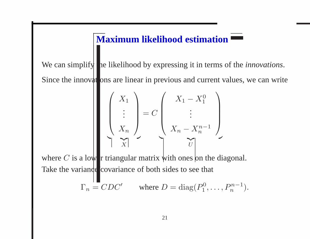
Maximum likelihood estimation
We can simplify the likelihood by expressing it in terms of the innovations.
Since the innovations are linear in previous and current values, we can write
X1
...
Xn
︸ ︷︷ ︸
X
= C
X1 −X01
...
Xn −Xn−1n
︸ ︷︷ ︸
U
whereC is a lower triangular matrix with ones on the diagonal.
Take the variance/covariance of both sides to see that
Γn = CDC ′ whereD = diag(P 01 , . . . , P
n−1n ).
21

Maximum likelihood estimation
Thus,|Γn| = |C|2P 01 · · ·Pn−1
n = P 01 · · ·Pn−1
n and
X ′Γ−1n X = U ′C ′Γ−1
n CU = U ′C ′C−TD−1C−1CU = U ′D−1U.
So we can rewrite the likelihood as
L(φ, θ, σ2w) =
1((2π)nP 0
1 · · ·Pn−1n
)1/2exp
(
−1
2
n∑
i=1
(Xi −Xi−1i )2/P i−1
i
)
=1
((2πσ2
w)nr01 · · · rn−1
n
)1/2exp
(
−S(φ, θ)2σ2
w
)
,
whereri−1i = P i−1
i /σ2w and
S(φ, θ) =n∑
i=1
(Xi −Xi−1
i
)2
ri−1i
.
22

Maximum likelihood estimation
The log likelihood ofφ, θ, σ2w is
l(φ, θ, σ2w) = log(L(φ, θ, σ2
w))
= −n2log(2πσ2
w)−1
2
n∑
i=1
log ri−1i − S(φ, θ)
2σ2w
.
Differentiating with respect toσ2w shows that the MLE(φ, θ, σ2
w) satisfies
n
2σ2w
=S(φ, θ)
2σ4w
⇔ σ2w =
S(φ, θ)
n,
andφ, θ minimize log
(
S(φ, θ)
n
)
+1
n
n∑
i=1
log ri−1i .
23

Summary: Maximum likelihood estimation
The MLE (φ, θ, σ2w) satisfies
σ2w =
S(φ, θ)
n,
andφ, θ minimize log
(
S(φ, θ)
n
)
+1
n
n∑
i=1
log ri−1i ,
whereri−1i = P i−1
i /σ2w and
S(φ, θ) =
n∑
i=1
(Xi −Xi−1
i
)2
ri−1i
.
24

Maximum likelihood estimation
Minimization is done numerically (e.g., Newton-Raphson).
Computational simplifications:
• Unconditional least squares.Drop thelog ri−1i terms.
• Conditional least squares.Also approximate the computation ofxi−1i by
dropping initial terms inS. e.g., for AR(2), all but the first two terms inS
depend linearly onφ1, φ2, so we have a least squares problem.
The differences diminish as sample size increases. For example,
P t−1t → σ2
w sort−1t → 1, and thusn−1
∑
i log ri−1i → 0.
25

Maximum likelihood estimation: Confidence intervals
For an ARMA(p,q) process, the MLE and un/conditional least
squares estimators satisfy
φ
θ
−
φ
θ
∼ AN
0,
σ2w
n
Γφφ Γφθ
Γθφ Γθθ,
−1
,
where
Γφφ Γφθ
Γθφ Γθθ,
= Cov((X, Y ), (X, Y )),
X = (X1, . . . , Xp)′ φ(B)Xt =Wt,
Y = (Y1, . . . , Yp)′ θ(B)Yt =Wt.
26
Introduction to Time Series Analysis. Lecture 12.
1. Review: Yule-Walker estimators
2. Yule-Walker example
3. Efficiency
4. Maximum likelihood estimation
5. Large-sample distribution of MLE
27