Intro to FEM

SorenBoettcher

Introduction to the Finite Element Method

Soren Boettcher

09.06.2009

Intro to FEM

SorenBoettcher

Outline

Motivation

Partial Differential Equations (PDEs)

Finite Difference Method (FDM)

Finite Element Method (FEM)

References

Intro to FEM

SorenBoettcher

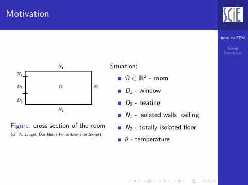
Motivation

Figure: cross section of the room(cf. A. Jungel, Das kleine Finite-Elemente-Skript)

Situation:

Ω ⊂ R2 - room

D1 - window

D2 - heating

N1 - isolated walls, ceiling

N2 - totally isolated floor

θ - temperature

Intro to FEM

SorenBoettcher

Motivation

Conservation of energy:∫ T

0

∫Ω

ρ0ce∂θ

∂tdx dt = −

∫ T

0

∫∂Ω

κ∂θ

∂νdσx dt +

∫ T

0

∫Ω

f dx dt

Heat equation:

ρ0ce∂θ

∂t− div(κ∇θ) = f in Ω for t > 0

Assumptions:

no time rate of change of the temperature, i.e. ∂θ∂t = 0

no interior heat source/sink, i.e. f = 0κ = 1

Intro to FEM

SorenBoettcher

Motivation

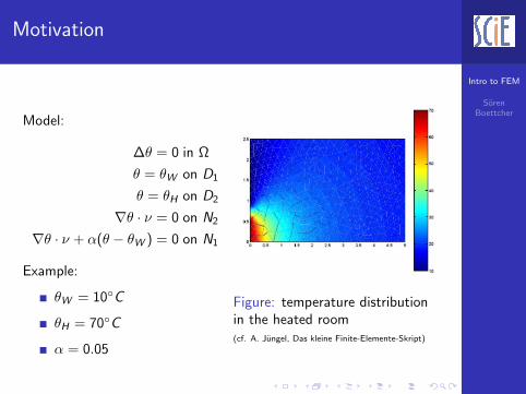
Model:

∆θ = 0 in Ω

θ = θW on D1

θ = θH on D2

∇θ · ν = 0 on N2

∇θ · ν + α(θ − θW ) = 0 on N1

Example:

θW = 10C

θH = 70C

α = 0.05

Figure: temperature distributionin the heated room(cf. A. Jungel, Das kleine Finite-Elemente-Skript)

Intro to FEM

SorenBoettcher

Partial Differential Equations (PDEs)

Second-order PDEs

Elliptic PDE (stationary) e.g. Poisson Equation (scalar)

−∆u = f in Ω

or stationary elasticity (vector-valued)

− div(σ) = f in Ω

Parabolic PDE e.g. heat equation

θ′ − div(κ∇θ) = f in Ω× (0,T )

Hyperbolic PDE e.g. instationary elasticity

u′′ − div(σ) = f in Ω× (0,T )

Intro to FEM

SorenBoettcher

Classification of PDEs

Linear PDE

θ′ −∆θ = f in Ω× (0,T )

Semilinear PDE

θ′ −∆θ = f (θ) in Ω× (0,T )

Quasilinear PDE

θ′ − div(α(∇θ)) = f in Ω× (0,T )

Fully nonlinear PDE

θ′ − g(∆θ) = f in Ω× (0,T )

Intro to FEM

SorenBoettcher

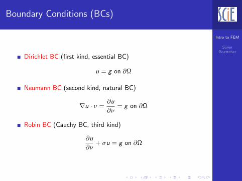
Boundary Conditions (BCs)

Dirichlet BC (first kind, essential BC)

u = g on ∂Ω

Neumann BC (second kind, natural BC)

∇u · ν =∂u

∂ν= g on ∂Ω

Robin BC (Cauchy BC, third kind)

∂u

∂ν+ σu = g on ∂Ω

Intro to FEM

SorenBoettcher

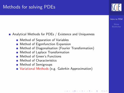
Methods for solving PDEs

Analytical Methods for PDEs / Existence and Uniqueness

Method of Separation of VariablesMethod of Eigenfunction ExpansionMethod of Diagonalisation (Fourier Transformation)Method of Laplace TransformationMethod of Green’s FunctionsMethod of CharacteristicsMethod of SemigroupsVariational Methods (e.g. Galerkin Approximation)

Intro to FEM

SorenBoettcher

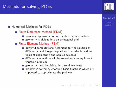
Methods for solving PDEs

Numerical Methods for PDEs

Finite Difference Method (FDM)

pointwise approximation of the differential equationgeometry is divided into an orthogonal grid

Finite Element Method (FEM)

powerful computational technique for the solution ofdifferential and integral equations that arise in variousfields of engineering and applied sciencesdifferential equations will be solved with an equivalentvariation problemgeometry must be divided into small elementsproblem is solved by choosing basis functions which aresupposed to approximate the problem

Intro to FEM

SorenBoettcher

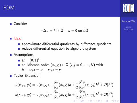
FDM

Consider

−∆u = f in Ω, u = 0 on ∂Ω

Idea:

approximate differential quotients by difference quotientsreduce differential equation to algebraic system

Assumptions:

Ω = (0, 1)2

equidistant nodes (xi , yj) ∈ Ω (i , j = 0, . . . ,N) withh = xi+1 − xi = yi+1 − yi

Taylor Expansion

u(xi+1, yj) = u(xi , yj) +∂u

∂x(xi , yj)h +

1

2

∂2u

∂x2(xi , yj)h

2 +O(h3)

u(xi−1, yj) = u(xi , yj)−∂u

∂x(xi , yj)h +

1

2

∂2u

∂x2(xi , yj)h

2 +O(h3)

Intro to FEM

SorenBoettcher

FDM

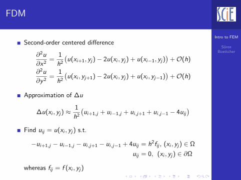
Second-order centered difference

∂2u

∂x2=

1

h2

(u(xi+1, yj)− 2u(xi , yj) + u(xi−1, yj)

)+O(h)

∂2u

∂y2=

1

h2

(u(xi , yj+1)− 2u(xi , yj) + u(xi , yj−1)

)+O(h)

Approximation of ∆u

∆u(xi , yj) ≈1

h2

(ui+1,j + ui−1,j + ui,j+1 + ui,j−1 − 4uij

)Find uij = u(xi , yj) s.t.

−ui+1,j − ui−1,j − ui,j+1 − ui,j−1 + 4uij = h2fij , (xi , yj) ∈ Ω

uij = 0, (xi , yj) ∈ ∂Ω

whereas fij = f (xi , yj)

Intro to FEM

SorenBoettcher

FDM

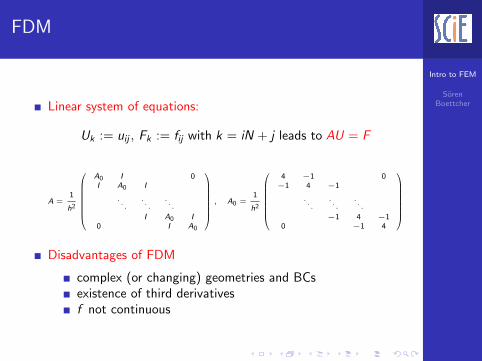
Linear system of equations:

Uk := uij , Fk := fij with k = iN + j leads to AU = F

A =1

h2

A0 I 0I A0 I

. . .. . .

. . .

I A0 I0 I A0

, A0 =1

h2

4 −1 0−1 4 −1

. . .. . .

. . .

−1 4 −10 −1 4

Disadvantages of FDM

complex (or changing) geometries and BCsexistence of third derivativesf not continuous

Intro to FEM

SorenBoettcher

FEM

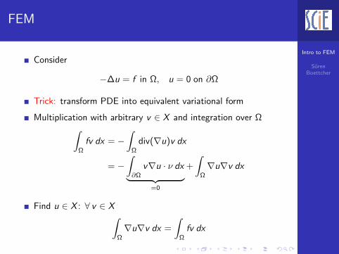
Consider

−∆u = f in Ω, u = 0 on ∂Ω

Trick: transform PDE into equivalent variational form

Multiplication with arbitrary v ∈ X and integration over Ω∫Ω

fv dx = −∫

Ω

div(∇u)v dx

= −∫∂Ω

v∇u · ν dx︸ ︷︷ ︸=0

+

∫Ω

∇u∇v dx

Find u ∈ X : ∀ v ∈ X∫Ω

∇u∇v dx =

∫Ω

fv dx

Intro to FEM

SorenBoettcher

FEM

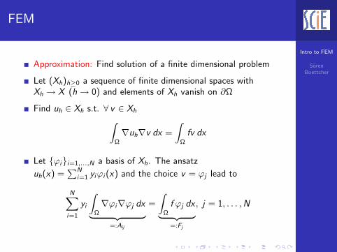
Approximation: Find solution of a finite dimensional problem

Let (Xh)h≥0 a sequence of finite dimensional spaces withXh → X (h→ 0) and elements of Xh vanish on ∂Ω

Find uh ∈ Xh s.t. ∀ v ∈ Xh∫Ω

∇uh∇v dx =

∫Ω

fv dx

Let ϕii=1,...,N a basis of Xh. The ansatz

uh(x) =∑N

i=1 yiϕi (x) and the choice v = ϕj lead to

N∑i=1

yi

∫Ω

∇ϕi∇ϕj dx︸ ︷︷ ︸=:Aij

=

∫Ω

f ϕj dx︸ ︷︷ ︸=:Fj

, j = 1, . . . ,N

Intro to FEM

SorenBoettcher

FEM

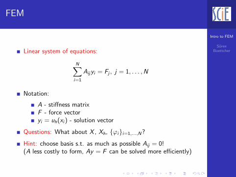
Linear system of equations:

N∑i=1

Aijyi = Fj , j = 1, . . . ,N

Notation:

A - stiffness matrixF - force vectoryi = uh(xi ) - solution vector

Questions: What about X , Xh, ϕii=1,...,N?

Hint: choose basis s.t. as much as possible Aij = 0!(A less costly to form, Ay = F can be solved more efficiently)

Intro to FEM

SorenBoettcher

FEM

Idea: discretise the domain into finite elements and define basisfunctions which vansih on most of these elements

1D: interval2D: triangular/quadrilateral shape3D: tetrahedral, hexahedral forms

Ansatz functions:

support of basis functions as small as possible and numberof basis functions whose supports intersect as small aspossibleuse of piecewise (images of) polynomials

Intro to FEM

SorenBoettcher

FEM

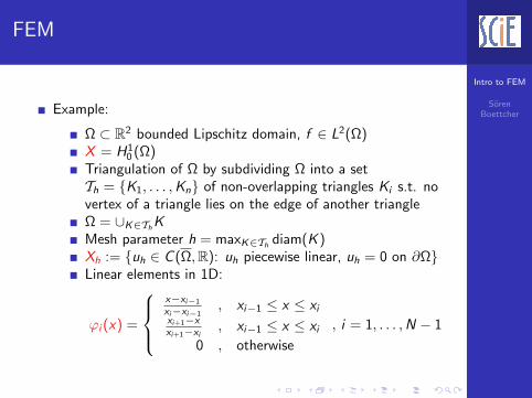
Example:

Ω ⊂ R2 bounded Lipschitz domain, f ∈ L2(Ω)X = H1

0 (Ω)Triangulation of Ω by subdividing Ω into a setTh = K1, . . . ,Kn of non-overlapping triangles Ki s.t. novertex of a triangle lies on the edge of another triangleΩ = ∪K∈Th

KMesh parameter h = maxK∈Th

diam(K )Xh := uh ∈ C (Ω,R): uh piecewise linear, uh = 0 on ∂ΩLinear elements in 1D:

ϕi (x) =

x−xi−1

xi−xi−1, xi−1 ≤ x ≤ xi

xi+1−xxi+1−xi

, xi−1 ≤ x ≤ xi

0 , otherwise

, i = 1, . . . ,N − 1

Intro to FEM

SorenBoettcher

FEM

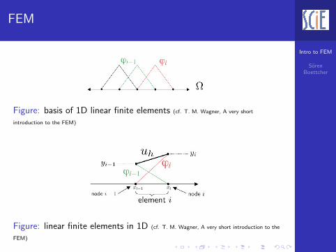
Figure: basis of 1D linear finite elements (cf. T. M. Wagner, A very short

introduction to the FEM)

Figure: linear finite elements in 1D (cf. T. M. Wagner, A very short introduction to the

FEM)

Intro to FEM

SorenBoettcher

FEM

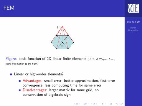
Figure: basis function of 2D linear finite elements (cf. T. M. Wagner, A very

short introduction to the FEM)

Linear or high-order elements?

Advantages: small error, better approximation, fast errorconvergence, less computing time for same errorDisadvantages: larger matrix for same grid, noconservation of algebraic sign

Intro to FEM

SorenBoettcher

FEM

Matrix A is large, but sparse: only a few matrix elements arenot equal to zero(intersection of the support of basis function is mostly empty)

A symmetric, positive definit unique solution

Linear system of equations: many methods in numerical linearalgebra exist to solve linear systems of equations

direct solvers (Gaussian elemination, LU decomposition,Cholesky decomposition): for N × N matrix ≈ N3

operationsiterative solvers (CG, GMRES, . . . ): ≈ N operations foreach iteration

Runge-Kutta methods (ODEs for unsteady problems)

Intro to FEM

SorenBoettcher

FEM

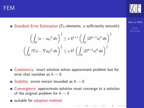
Standard Error Estimation (Pk -elements, u sufficiently smooth):(∫Ω

|u − uh|2 dx

) 12

≤ c hk+1

(∫Ω

|Dk+1u|2 dx

) 12

(∫Ω

|∇u −∇uh|2 dx

) 12

≤ c hk

(∫Ω

|Dk+1u|2 dx

) 12

Consistency: exact solution solves approximate problem but forerror that vanishes as h→ 0

Stability: errors remain bounded as h→ 0

Convergence: approximate solution must converge to a solutionof the original problem for h→ 0

suitable for adaptive method

Intro to FEM

SorenBoettcher

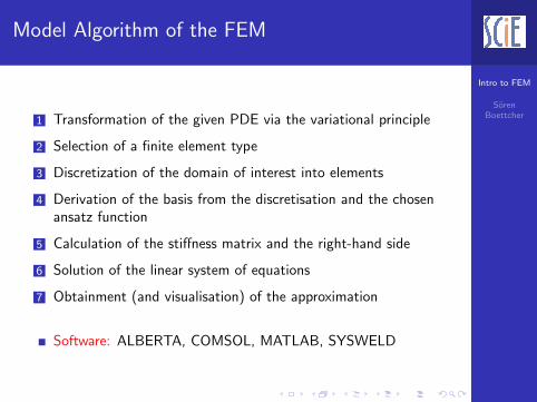
Model Algorithm of the FEM

1 Transformation of the given PDE via the variational principle

2 Selection of a finite element type

3 Discretization of the domain of interest into elements

4 Derivation of the basis from the discretisation and the chosenansatz function

5 Calculation of the stiffness matrix and the right-hand side

6 Solution of the linear system of equations

7 Obtainment (and visualisation) of the approximation

Software: ALBERTA, COMSOL, MATLAB, SYSWELD

Intro to FEM

SorenBoettcher

References

K. Atkinson, W. Han; Theoretical Numerical Analysis.

D. Braess; Finite Elements.

R. Dautray, J.-L. Lions; Mathematical Analysis and NumericalMethods for Science and Technology, Vol. 6: Evolution Problems II.

C. Grossmann, H.-G. Roos; Numerical Treatment of PDEs.

K. Knothe, H. Wessels; Finite elements.

G. R. Liu, S. S. Quek; The FEM.

M. Renardy, R. C. Rogers; An Introduction to PDEs.

E. G. Thompson; Introduction to the FEM.

Intro to FEM

SorenBoettcher

Thank you for your attention.