Embed Size (px)
Citation preview
Introduction to Statistics
Class Overheadsfor
APA 3381“Measurement and Data Analysis
in Human Kinetics”
byD. Gordon E. Robertson, PhD, FCSB
School of Human KineticsUniversity of Ottawa
Copyright © D.G.E. Robertson, September 2015
2
Introduction to Statistics
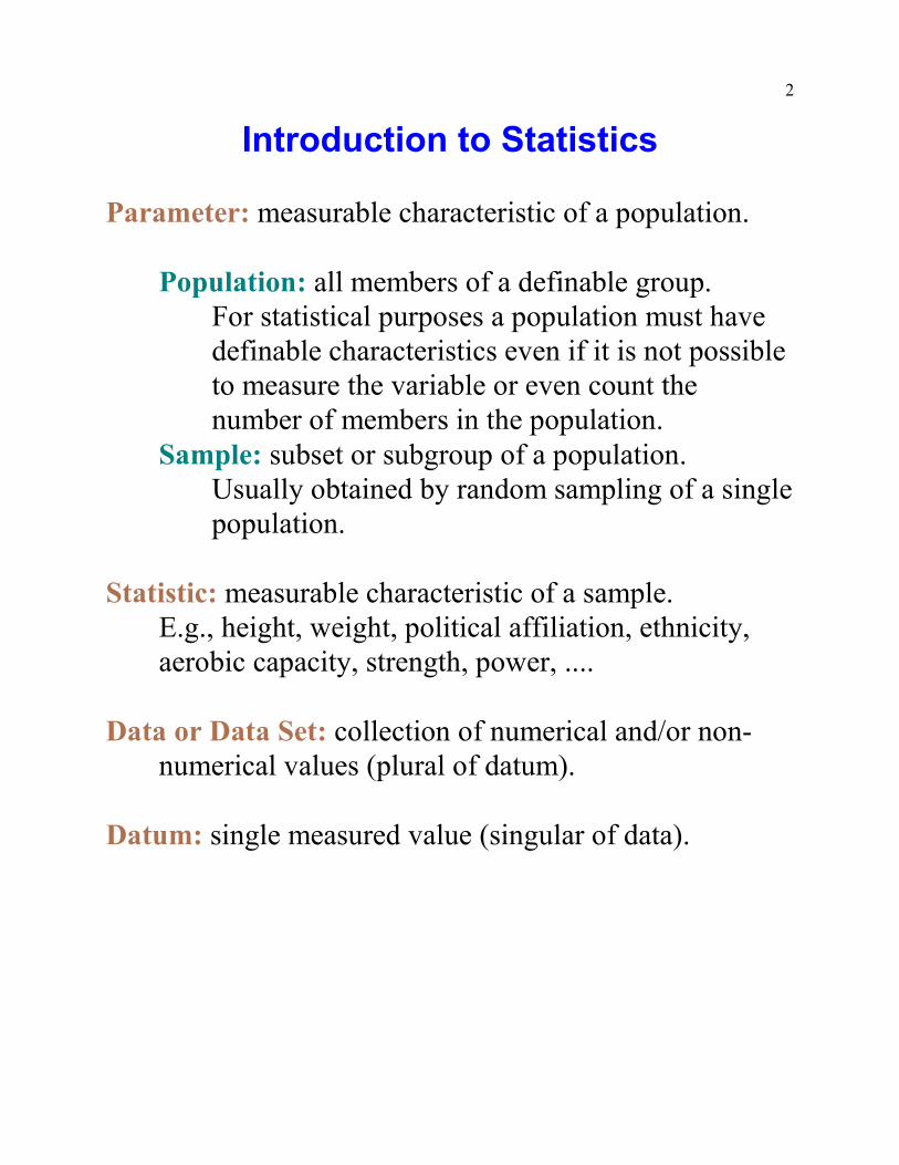
Parameter: measurable characteristic of a population.
Population: all members of a definable group.For statistical purposes a population must havedefinable characteristics even if it is not possibleto measure the variable or even count thenumber of members in the population.
Sample: subset or subgroup of a population.Usually obtained by random sampling of a singlepopulation.
Statistic: measurable characteristic of a sample.E.g., height, weight, political affiliation, ethnicity,aerobic capacity, strength, power, ....
Data or Data Set: collection of numerical and/or non-numerical values (plural of datum).
Datum: single measured value (singular of data).
3
Statistics
Statistics: 1. plural of statistic, 2. science of conductingstudies to collect, organize, summarize, analyze and drawconclusions from data.
Descriptive statistics: collection, description,organization, presentation and analysis of data.
Inferential statistics: generalizing from samples topopulations, testing of hypotheses, determiningrelationships among variables and making decisions,uses probability theory to make decisions.
Hypothesis: “less than a thesis”, a testableconjecture based on a theory.Thesis: a dissertation or learned argument whichdefends a particular proposition or theory.
Qualitative measurements:typically non-numerical, subjectively measured,
judgmentally determined, categorical.E.g., religious affiliation, teacher/professor
evaluations, emotional states, flavour, gender.
Quantitative measurements:typically numerical, objectively measured, reliability
(repeatability or precision) and validity (accuracy) can beevaluated against a criterion.
E.g., salary, course grade, foot size, IQ, age, girth.
4
Types of quantitative measures:Constants: quantities with fixed characteristics.
Physical constants: G, c, h (Planck’s constant)Mathematical constants: p, e, i
Variables: quantities whose characteristics vary.Discrete variables: numerical variables that
have finitely many possibilities (usuallyintegers), countable many possible values
Examples: value of $ bills or coins, card countContinuous variables: numerical variables that
have infinitely many possible values withina range of values (numbers between –1 and+1) or unbounded (Real numbers, numbersgreater than 0).
Examples: height, duration, angle (only a fixednumber of significant figures are reported).
Significant Figures:When reporting numerical information, especially whenobtained by a calculator, usually only 3 or 4 digits arerequired. The general rule that is accurate to 0.5% holdsthat only 4 significant figures are needed if the firstnonzero number is a 1 and 3 when it is not.Examples: 234 000, 1.234, 2.45, 0.003 45, 0.1234,
8910, and 56 100.Exceptions are frequencies and counts when all digits arereported and financial numbers, hich are too nearestdollar or nearest cent depending on the amount.
5
Measurement Scales
Nominal: classifies data into mutually exclusive(nonoverlapping), exhaustive categories in which noordering or ranking of the categories is implied.
E.g., colour, flavour, religion, gender, sex,nationality, county of residence, postal code.
Ordinal: classifies data into categories that can beordered or ranked (highest to lowest or vice versa),precise differences between categories does not exist.
E.g., teaching evaluations, letter grade (A+, A, A–, ...F), judges scores (0–10), preferences (polls), skillrankings.
Interval: numerical data with precise differences betweencategories but with no true zero (i.e., zero implies absenceof quantity).
E.g., IQ (0 means could not be measured),temperature (degrees Celsius), z-scores (0 is averagevalue), acidity (pH, 7 is neutral).
Ratio: interval data with a true zero, true ratios existE.g., height, weight, temperature (in Kelvins),
strength, price, age, duration.
6
Methods of Sampling
Random: subjects are randomly selected from apopulation, all subjects have equal probability of beingselected, subjects may not be selected twice.
Systematic: subjects are numbered sequentially andevery n subject is selected to obtain a sample of N/nth
subjects (N is number of people in population).
Stratified: population is divided into identifiable groups(strata) by some relevant variable (income, gender, age,education) and each strata is sampled randomly inproportion to the strata’s relative size in the population.
Cluster: subjects are randomly sampled fromrepresentative clusters or regions of the population.Economical method if subjects are widely dispersedgeographically.
Convenience: typically used in student projects and byjournalists, uses subjects that can be conveniently polledor tested. Not suitable for pollsters or medical research.
7
Graphing 1
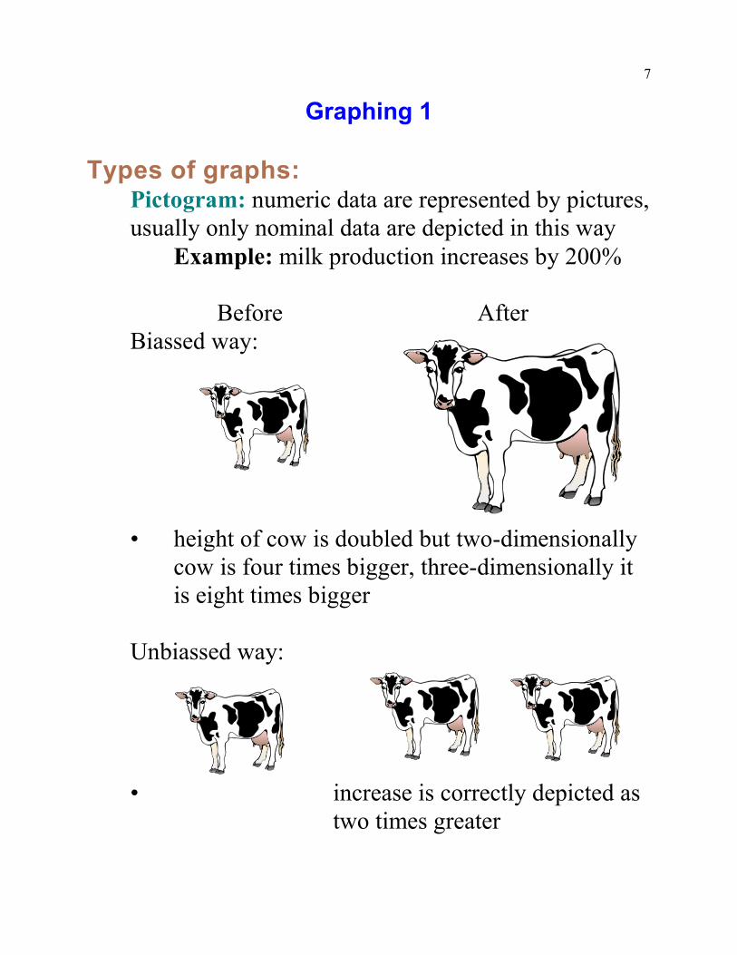
Types of graphs:Pictogram: numeric data are represented by pictures,usually only nominal data are depicted in this way
Example: milk production increases by 200%
Before AfterBiassed way:
• height of cow is doubled but two-dimensionallycow is four times bigger, three-dimensionally itis eight times bigger
Unbiassed way:
• increase is correctly depicted astwo times greater
8
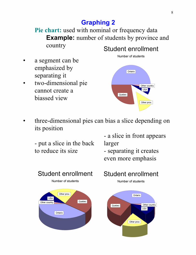
Graphing 2Pie chart: used with nominal or frequency data
Example: number of students by province andcountry
• a segment can beemphasized byseparating it
• two-dimensional piecannot create abiassed view
• three-dimensional pies can bias a slice depending onits position
- a slice in front appears- put a slice in the back largerto reduce its size - separating it creates
even more emphasis
9
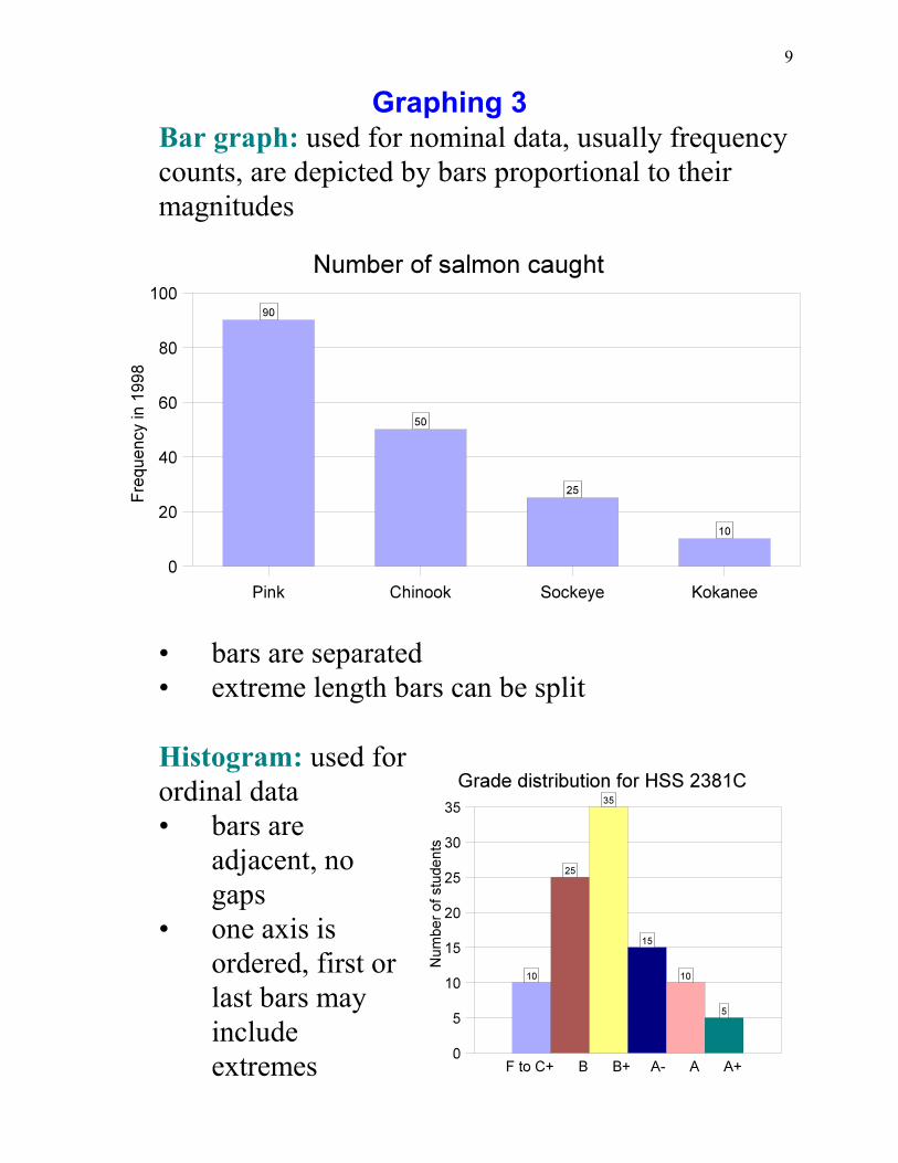
Graphing 3Bar graph: used for nominal data, usually frequencycounts, are depicted by bars proportional to theirmagnitudes
• bars are separated• extreme length bars can be split
Histogram: used forordinal data• bars are
adjacent, nogaps
• one axis isordered, first orlast bars mayincludeextremes
10
Graphing 4
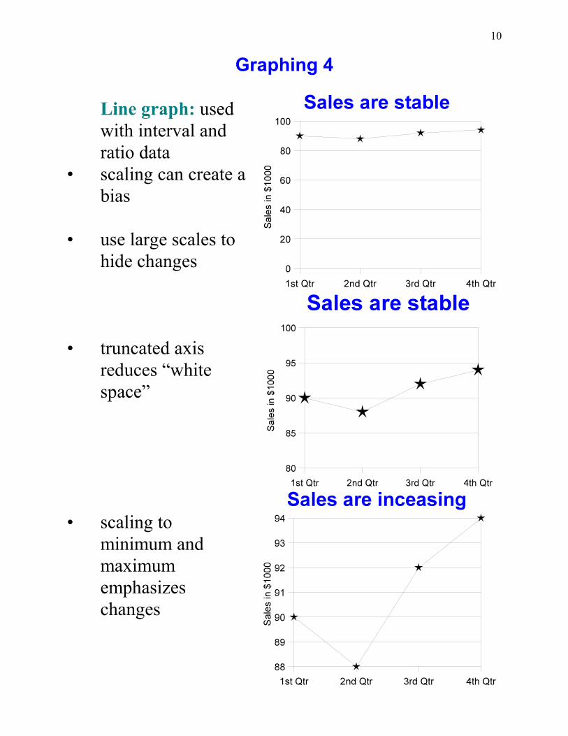
Line graph: usedwith interval andratio data
• scaling can create abias
• use large scales tohide changes
• truncated axisreduces “whitespace”
• scaling tominimum andmaximumemphasizeschanges
11
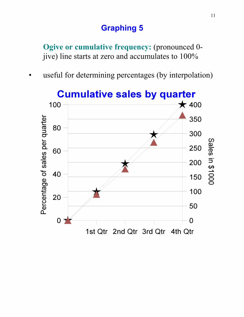
Graphing 5
Ogive or cumulative frequency: (pronounced 0-jive) line starts at zero and accumulates to 100%
• useful for determining percentages (by interpolation)
12
Rules for Constructing a Frequency Histogram
1. There should be between 5 and 20 classes.• this is strictly for aesthetic purposes
2. The class width should be an odd number.• this ensures that the midpoint has the same number of
decimal places as the original data
3. The classes must be mutually exclusive.• each datum must fall into one class and one class only
4. The classes must be continuous.• there should be no “gaps” in the number line even if a
class has no members
5. The classes must be exhaustive.• all possible data must fit into one of the classes
6. The classes must have equal width.• if not there will be a bias among the classes• you can have open-ended classes at the ends (i.e., for
ages you may use 10 and under or 65 and over, etc.)
13
Types of Frequency Distributions
Categorical - for nominal types of data
Ungrouped - for numerical data with few scores
Grouped - for numerical data with many scores
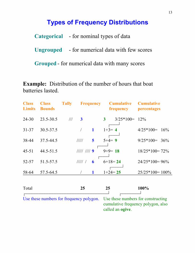
Example: Distribution of the number of hours that boatbatteries lasted.
Class Class Tally Frequency Cumulative CumulativeLimits Bounds frequency percentages
24-30 23.5-30.5 /// 3 3 3/25*100= 12% +)))-
31-37 30.5-37.5 / 1 1+3= 4 4/25*100= 16% +)))-
38-44 37.5-44.5 ///// 5 5+4= 9 9/25*100= 36% +)))-
45-51 44.5-51.5 ///// //// 9 9+9= 18 18/25*100= 72% +)))-
52-57 51.5-57.5 ///// / 6 6+18= 24 24/25*100= 96% +))))-
58-64 57.5-64.5 / 1 1+24= 25 25/25*100= 100%
Total 25 25 100%+))))))))))))))))))))))))))))))))- +)))))))-Use these numbers for frequency polygon. Use these numbers for constructing
cumulative frequency polygon, alsocalled an ogive.
14
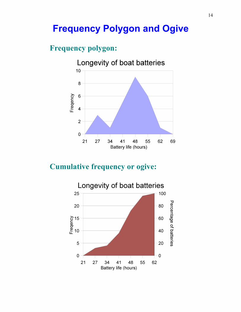
Frequency Polygon and Ogive
Frequency polygon:
Cumulative frequency or ogive:
15
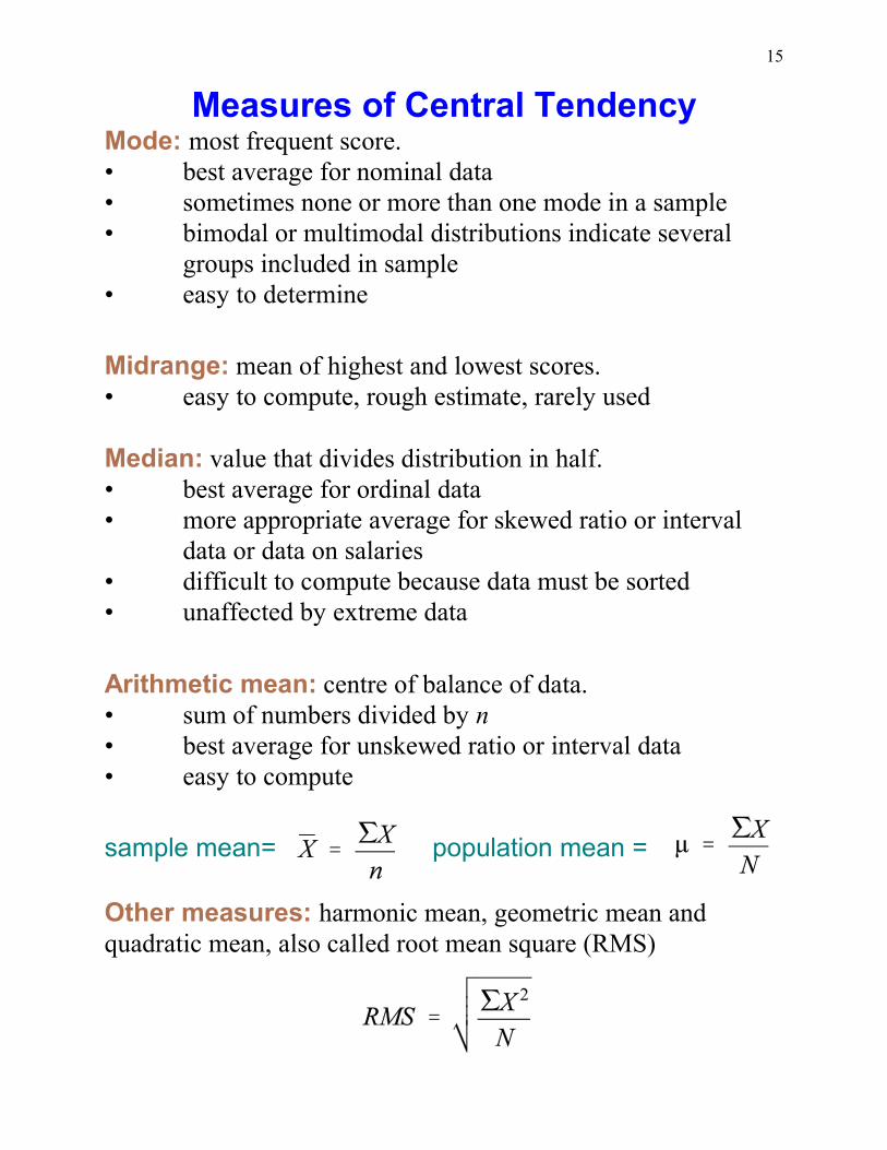
Measures of Central TendencyMode: most frequent score.• best average for nominal data• sometimes none or more than one mode in a sample• bimodal or multimodal distributions indicate several
groups included in sample• easy to determine
Midrange: mean of highest and lowest scores.• easy to compute, rough estimate, rarely used
Median: value that divides distribution in half.• best average for ordinal data• more appropriate average for skewed ratio or interval
data or data on salaries• difficult to compute because data must be sorted• unaffected by extreme data
Arithmetic mean: centre of balance of data.• sum of numbers divided by n• best average for unskewed ratio or interval data• easy to compute
sample mean= population mean =
Other measures: harmonic mean, geometric mean andquadratic mean, also called root mean square (RMS)
16
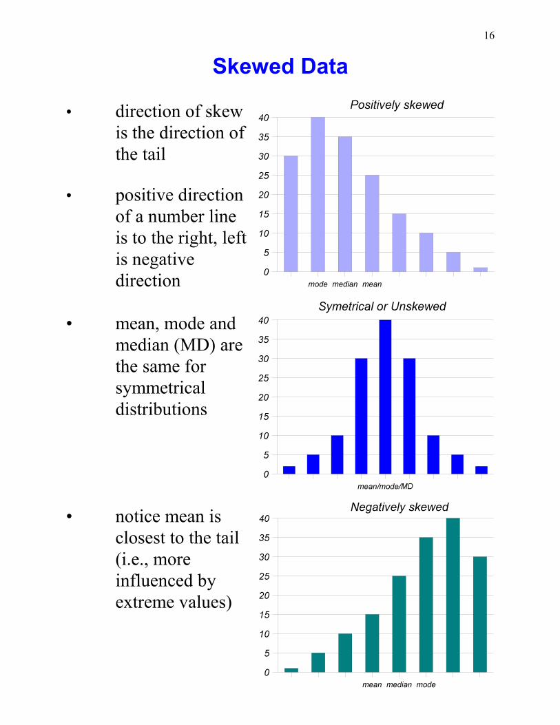
Skewed Data
• direction of skewis the direction ofthe tail
• positive directionof a number lineis to the right, leftis negativedirection
• mean, mode andmedian (MD) arethe same forsymmetricaldistributions
• notice mean isclosest to the tail(i.e., moreinfluenced byextreme values)
17
Measures of Variation
Range: highest minus lowest values.• used for ordinal data
R = highest – lowest
Interquartile range: 75 minus 25 percentile.th th
• used for determining “outliers”
3 1IQR = Q – Q
Variance: mean of squared differences between scores and
the mean value (m).• used on ratio or interval data• used for advanced statistical analysis (ANOVAs)
Standard deviation: has same units as raw data.• used on ratio or interval data• most commonly used measure of variation
Coefficient of variation: percentage of standard deviationto mean.
• used to compare variability among data with differentunits of measure. Not suitable for interval data.
18
Biased and Unbiased Estimators
• sample mean is an unbiased estimate of the populationmean (m)
• variances and standard deviations are biased estimatorsbecause mean is used in their computation
Why?• Last score can be determined from mean and all other
scores, therefore, it is not free to vary or add tovariability. To compensate divide sums of squares byn–1 instead of n.
• Instead of using the standard formula a computingformula is used so that running totals of scores andscores squared may be used to compute variability.
Computing Formulae
Variance: s = sample variance2
Standard deviation: S = sample standard deviation
19
Measures of Position
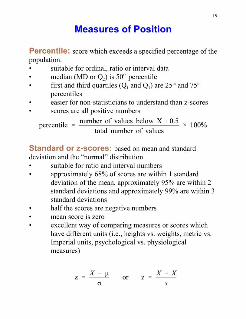
Percentile: score which exceeds a specified percentage of thepopulation.• suitable for ordinal, ratio or interval data
2• median (MD or Q ) is 50 percentileth
1 3• first and third quartiles (Q and Q ) are 25 and 75th th
percentiles• easier for non-statisticians to understand than z-scores• scores are all positive numbers
Standard or z-scores: based on mean and standarddeviation and the “normal” distribution.• suitable for ratio and interval numbers• approximately 68% of scores are within 1 standard
deviation of the mean, approximately 95% are within 2standard deviations and approximately 99% are within 3standard deviations
• half the scores are negative numbers• mean score is zero• excellent way of comparing measures or scores which
have different units (i.e., heights vs. weights, metric vs.Imperial units, psychological vs. physiologicalmeasures)
20
Measures of Position and Outliers
Other measures of position:Deciles: 1 2 10 10 , 20 , ... 100 percentiles (D , D , ...D )th th th
• often used in education or demographic studies
Quartiles: 1 2 3 25 , 50 and 75 percentiles (Q , Q , Q )th th th
• frequently used for exploratory statistics and to
2determine outliers (Q is same as median)
Outliers: extreme values that adversely affect statisticalmeasures of central tendency and variation.
Method of determining outliers:• compute interquartile range (IRQ)• multiply IRQ by 1.5
1• lower bound is Q minus 1.5 × IRQ
3• upper bound is Q plus 1.5 × IRQ• values outside these bounds are outliers and may be
removed from the data set• it is assumed that outliers are the result of errors in
measurement or recording or were taken from anunrepresentative individual
Alternate method for normally distributed data:• +/– 4 or 5 standard deviations
21
Counting Techniques
Fundamental Counting Rule:In a sequence of “n” events with each event having “k”
possibilities, the total number of outcomes is:k = k × k × k × . . . × kn
Examples:• How many 6 digit student ID numbers
10 × 10 × 10 × 10 × 10 × 10 = 1 000 000
• How many ways of throwing 5 dice (Yahtze) 6 × 6 × 6 × 6 × 6 = 7 776
• How many ways of selecting 3 letters 26 × 26 × 26 = 17 576
1In a sequence of “n” events in which there are “k ” possibilities
2for the first event, “k ” possibilities for the second event and
3“k ” for the third, etc., the total number of possible outcomes is:
1 2 3 nk × k × k × . . . × kExamples:• How many 3 digit phone exchanges before 1980
8 × 2 × 10 = 160 (minus 911, 311, 411, 511)
• How many 3 digit phone exchanges after 19808 × 10 × 10 = 800 (minus 911, 311, 411, 511)
• How many 7 character Ontario licence plates (4letters, 3 numbers)26 × 26 × 26 × 26 × 10 × 10 × 10 = 456 976 000
22
Factorial Notation
Factorials:Factorial numbers are identified with an exclamation
mark (n!). They are defined:
n! = n × n–1 × n–2 × . . . × 1
0! is defined to be 1
Examples: 1! = 1
2! = 2 × 1 = 2
5! = 5 × 4 × 3 × 2 × 1 = 120
12! = 479 001 600
20! . 2.433 × 10¹⁸
23
Permutations and Combinations 1
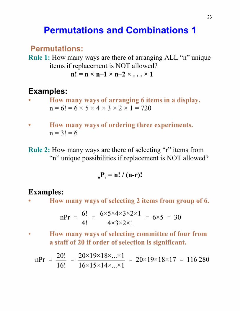
Permutations:Rule 1: How many ways are there of arranging ALL “n” unique
items if replacement is NOT allowed?n! = n × n–1 × n–2 × . . . × 1
Examples:• How many ways of arranging 6 items in a display.
n = 6! = 6 × 5 × 4 × 3 × 2 × 1 = 720
• How many ways of ordering three experiments.n = 3! = 6
Rule 2: How many ways are there of selecting “r” items from“n” unique possibilities if replacement is NOT allowed?
n rP = n! / (n-r)!
Examples:• How many ways of selecting 2 items from group of 6.
• How many ways of selecting committee of four froma staff of 20 if order of selection is significant.
24
Permutations and Combinations 2
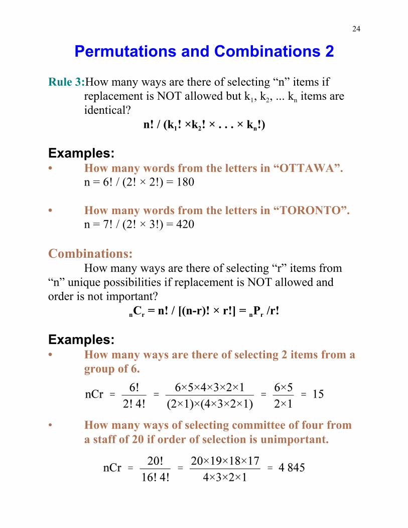
Rule 3:How many ways are there of selecting “n” items if
1 2 nreplacement is NOT allowed but k , k , ... k items areidentical?
1 2 nn! / (k ! ×k ! × . . . × k !)
Examples:• How many words from the letters in “OTTAWA”.
n = 6! / (2! × 2!) = 180
• How many words from the letters in “TORONTO”.n = 7! / (2! × 3!) = 420
Combinations:How many ways are there of selecting “r” items from
“n” unique possibilities if replacement is NOT allowed andorder is not important?
n r n rC = n! / [(n-r)! × r!] = P /r!
Examples:• How many ways are there of selecting 2 items from a
group of 6.
• How many ways of selecting committee of four froma staff of 20 if order of selection is unimportant.
25
Probability
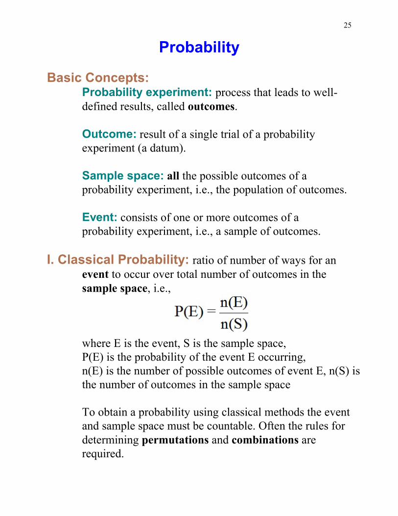
Basic Concepts:Probability experiment: process that leads to well-defined results, called outcomes.
Outcome: result of a single trial of a probabilityexperiment (a datum).
Sample space: all the possible outcomes of aprobability experiment, i.e., the population of outcomes.
Event: consists of one or more outcomes of aprobability experiment, i.e., a sample of outcomes.
I. Classical Probability: ratio of number of ways for anevent to occur over total number of outcomes in thesample space, i.e.,
where E is the event, S is the sample space,P(E) is the probability of the event E occurring,n(E) is the number of possible outcomes of event E, n(S) isthe number of outcomes in the sample space
To obtain a probability using classical methods the eventand sample space must be countable. Often the rules fordetermining permutations and combinations arerequired.
26
Classical Probability 1
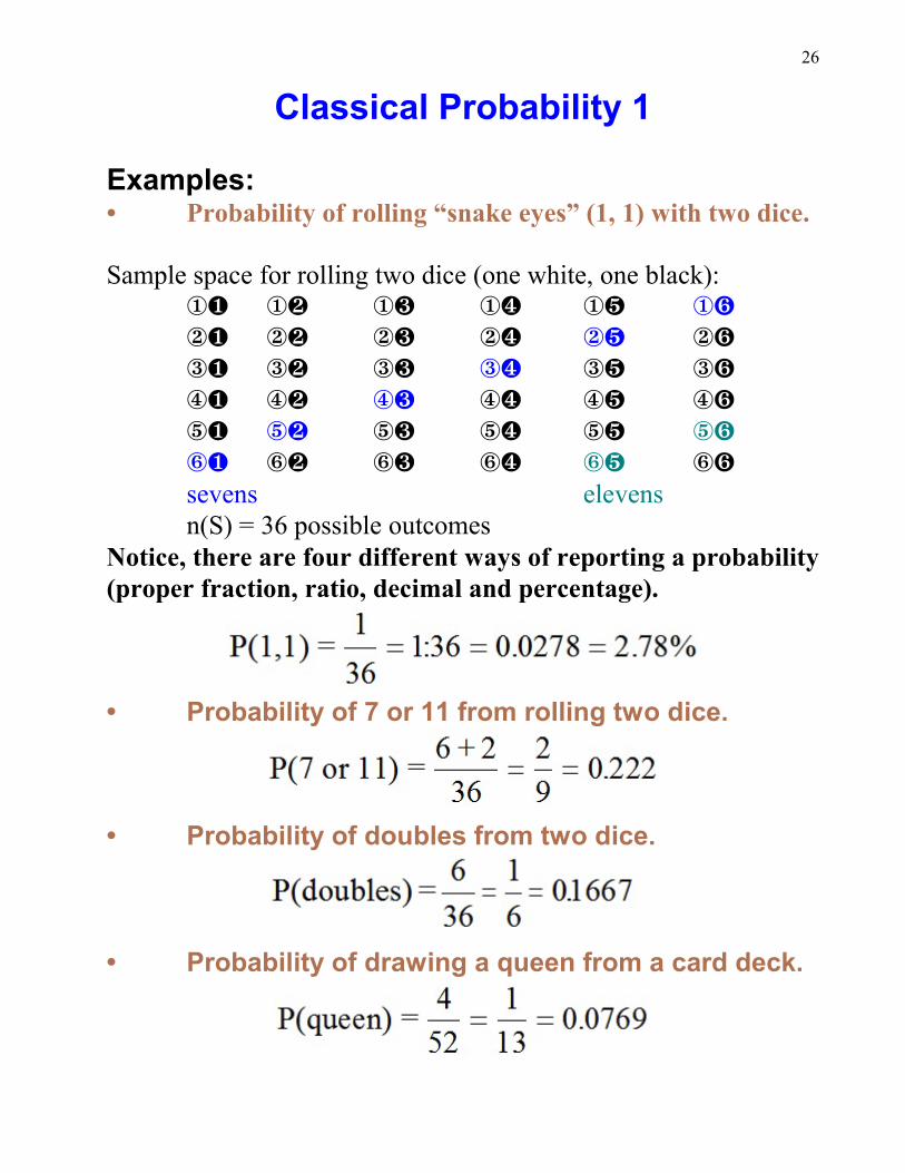
Examples:• Probability of rolling “snake eyes” (1, 1) with two dice.
Sample space for rolling two dice (one white, one black):ÎØ ÎÙ ÎÚ ÎÛ ÎÜ ÎÝÏØ ÏÙ ÏÚ ÏÛ ÏÜ ÏÝÐØ ÐÙ ÐÚ ÐÛ ÐÜ ÐÝÑØ ÑÙ ÑÚ ÑÛ ÑÜ ÑÝÒØ ÒÙ ÒÚ ÒÛ ÒÜ ÒÝÓØ ÓÙ ÓÚ ÓÛ ÓÜ ÓÝsevens elevensn(S) = 36 possible outcomes
Notice, there are four different ways of reporting a probability(proper fraction, ratio, decimal and percentage).
• Probability of 7 or 11 from rolling two dice.
• Probability of doubles from two dice.
• Probability of drawing a queen from a card deck.
27
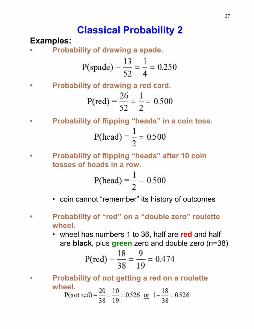
Classical Probability 2Examples:• Probability of drawing a spade.
• Probability of drawing a red card.
• Probability of flipping “heads” in a coin toss.
• Probability of flipping “heads” after 10 cointosses of heads in a row.
• coin cannot “remember” its history of outcomes
• Probability of “red” on a “double zero” roulettewheel.• wheel has numbers 1 to 36, half are red and half
are black, plus green zero and double zero (n=38)
• Probability of not getting a red on a roulettewheel.
28
Rules of Probability
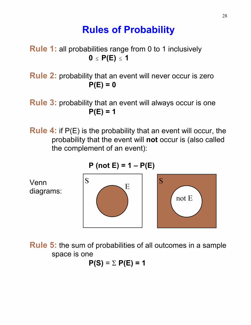
Rule 1: all probabilities range from 0 to 1 inclusively0 # P(E) # 1
Rule 2: probability that an event will never occur is zeroP(E) = 0
Rule 3: probability that an event will always occur is oneP(E) = 1
Rule 4: if P(E) is the probability that an event will occur, theprobability that the event will not occur is (also calledthe complement of an event):
P (not E) = 1 – P(E)
Venn diagrams:
Rule 5: the sum of probabilities of all outcomes in a samplespace is one
P(S) = S P(E) = 1

29
Empirical Probability
II. Empirical Probability: obtained empirically bysampling a population and creating a representativefrequency distribution.• for a given frequency distribution, probability is the
ratio of frequency of an event class to the totalnumber of data in the frequency distribution, i.e.,
Examples:• Probability of a girl baby.
Assume that a population has a blood type distribution of:2% AB, 5% B, 23% A, and 70% O
• Probability of a person having type B or ABblood.
P(AB or B) = 2% + 5% = 7.00% = 0.0700
• Probability of strongly left-handed person.
P(strongly left-handed) = 0.050 = 5.00%
• Probability of “natural” blues eyes.
P(blues eyes) = 0.065 = 6.50%
30
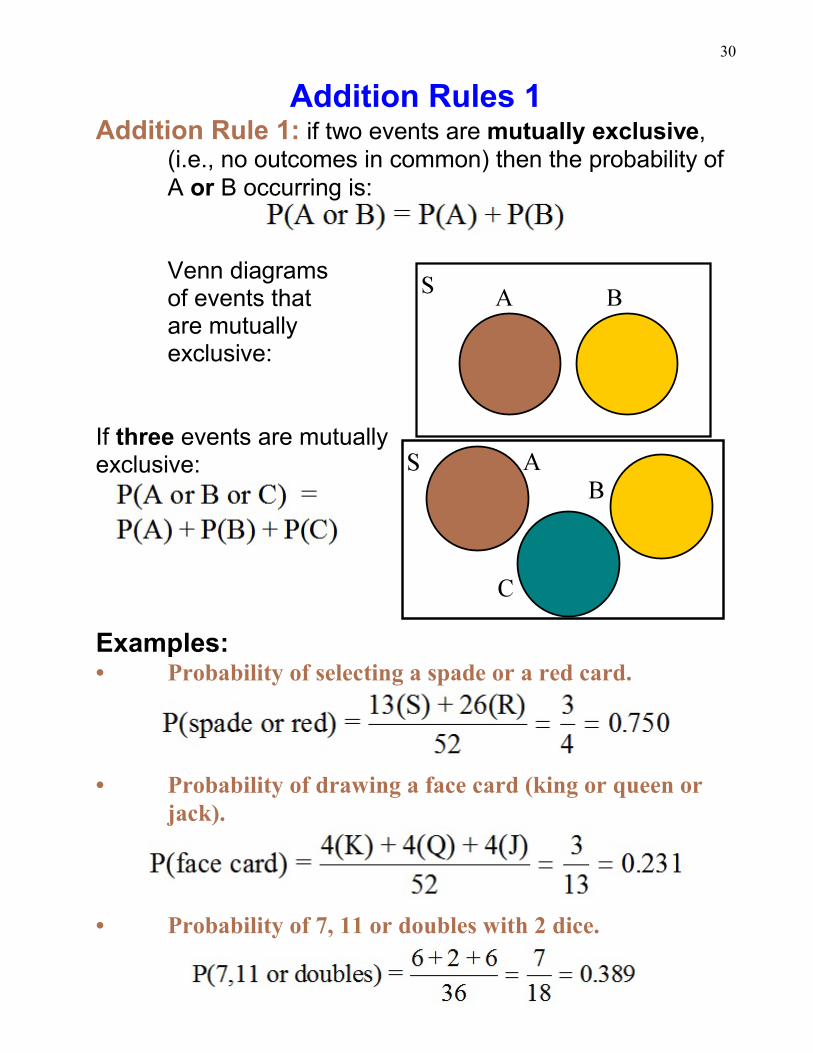
Addition Rules 1Addition Rule 1: if two events are mutually exclusive,
(i.e., no outcomes in common) then the probability ofA or B occurring is:
Venn diagramsof events thatare mutuallyexclusive:
If three events are mutually exclusive:
Examples:• Probability of selecting a spade or a red card.
• Probability of drawing a face card (king or queen orjack).
• Probability of 7, 11 or doubles with 2 dice.
31
Addition Rules 2
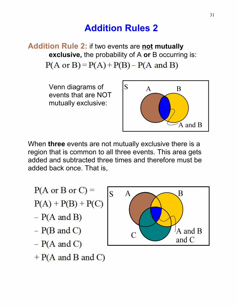
Addition Rule 2: if two events are not mutuallyexclusive, the probability of A or B occurring is:
Venn diagrams ofevents that are NOTmutually exclusive:
When three events are not mutually exclusive there is aregion that is common to all three events. This area getsadded and subtracted three times and therefore must beadded back once. That is,
32
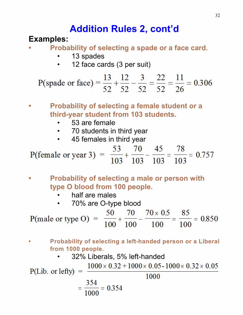
Addition Rules 2, cont’dExamples:• Probability of selecting a spade or a face card.
• 13 spades• 12 face cards (3 per suit)
• Probability of selecting a female student or athird-year student from 103 students.
• 53 are female• 70 students in third year• 45 females in third year
• Probability of selecting a male or person withtype O blood from 100 people.
• half are males • 70% are O-type blood
• Probability of selecting a left-handed person or a Liberal
from 1000 people.
• 32% Liberals, 5% left-handed
33
IndependenceDefinition: two events are independent if the occurrence
of one event has no effect on the occurrence of theother event. In probability experiments where there isno “memory” from one event to the next, the eventsare called independent.
Examples of Independent Events:Coin tosses. Even when 10 heads are flipped in a row the next
coin toss still as a 50:50 chance of being a head.
Roulette wheel spins. Each spin of the wheel is theoreticallyindependent. Each number on the wheel has equalprobability of occurring at each spin.
Rolling dice repeatedly. The dice cannot “remember” whatthey rolled from one toss to another.
Drawing cards with replacement. “With replacement”means after a card is drawn it is put back in the deck; thusall cards are equally likely to be drawn each time.
Examples of Dependent Events:Drawing cards without replacement. Once a card is drawn
it cannot be drawn a second time. This changes thecharacteristics of the remaining deck of cards.
Bingo numbers. Once a ball is drawn it is not replaced.
Lottery 6/49. All numbers (1– 49) are equally likely to bechosen but can only be chosen once.
34
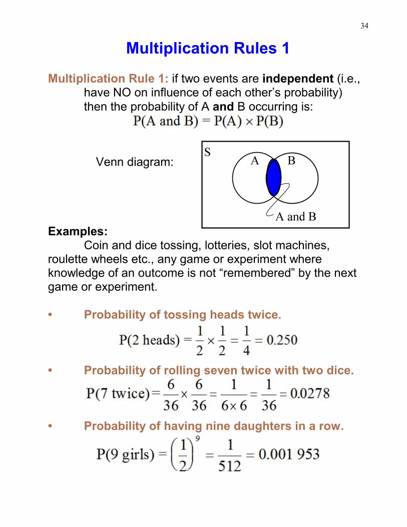
Multiplication Rules 1
Multiplication Rule 1: if two events are independent (i.e.,have NO on influence of each other’s probability)then the probability of A and B occurring is:
Venn diagram:
Examples:Coin and dice tossing, lotteries, slot machines,
roulette wheels etc., any game or experiment whereknowledge of an outcome is not “remembered” by the nextgame or experiment.
• Probability of tossing heads twice.
• Probability of rolling seven twice with two dice.
• Probability of having nine daughters in a row.
35
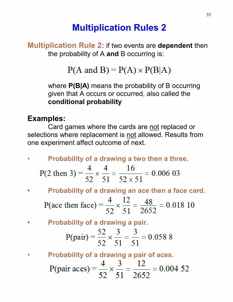
Multiplication Rules 2
Multiplication Rule 2: if two events are dependent thenthe probability of A and B occurring is:
where P(B|A) means the probability of B occurringgiven that A occurs or occurred, also called theconditional probability
Examples:Card games where the cards are not replaced or
selections where replacement is not allowed. Results fromone experiment affect outcome of next.
• Probability of a drawing a two then a three.
• Probability of a drawing an ace then a face card.
• Probability of a drawing a pair.
• Probability of a drawing a pair of aces.
36
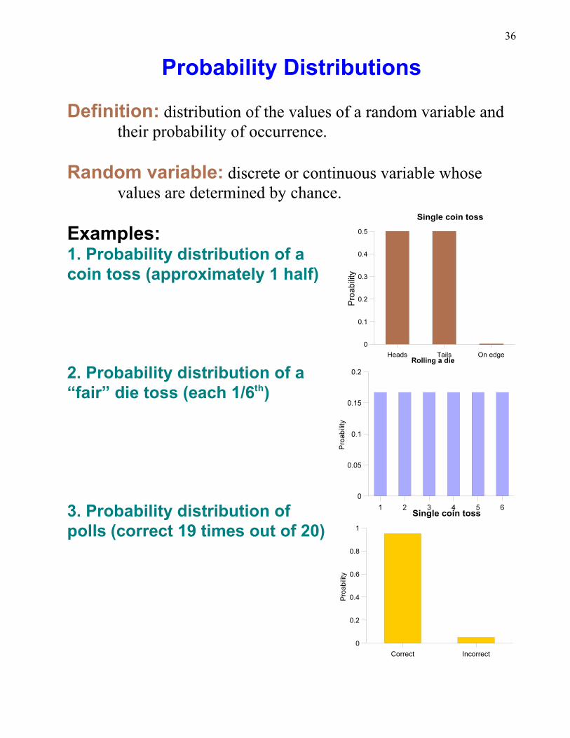
Probability Distributions
Definition: distribution of the values of a random variable andtheir probability of occurrence.
Random variable: discrete or continuous variable whosevalues are determined by chance.
Examples:1. Probability distribution of acoin toss (approximately 1 half)
2. Probability distribution of a “fair” die toss (each 1/6 )th
3. Probability distribution ofpolls (correct 19 times out of 20)
37
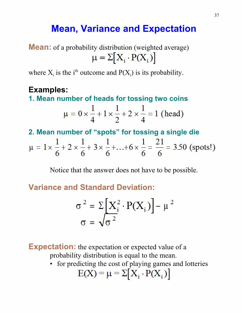
Mean, Variance and Expectation
Mean: of a probability distribution (weighted average)
i iwhere X is the i outcome and P(X ) is its probability.th
Examples:1. Mean number of heads for tossing two coins
2. Mean number of “spots” for tossing a single die
Notice that the answer does not have to be possible.
Variance and Standard Deviation:
Expectation: the expectation or expected value of aprobability distribution is equal to the mean.• for predicting the cost of playing games and lotteries
38
Expectation cont’d
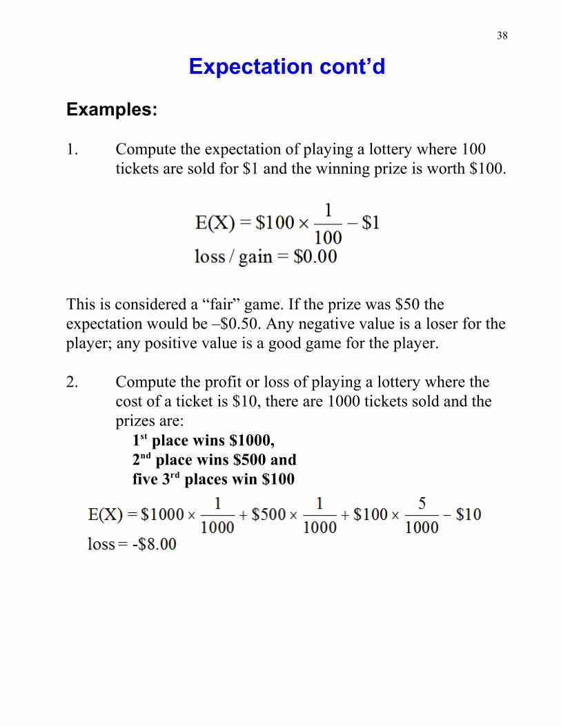
Examples:
1. Compute the expectation of playing a lottery where 100tickets are sold for $1 and the winning prize is worth $100.
This is considered a “fair” game. If the prize was $50 theexpectation would be –$0.50. Any negative value is a loser for theplayer; any positive value is a good game for the player.
2. Compute the profit or loss of playing a lottery where thecost of a ticket is $10, there are 1000 tickets sold and theprizes are:
1 place wins $1000,st
2 place wins $500 andnd
five 3 places win $100rd
39
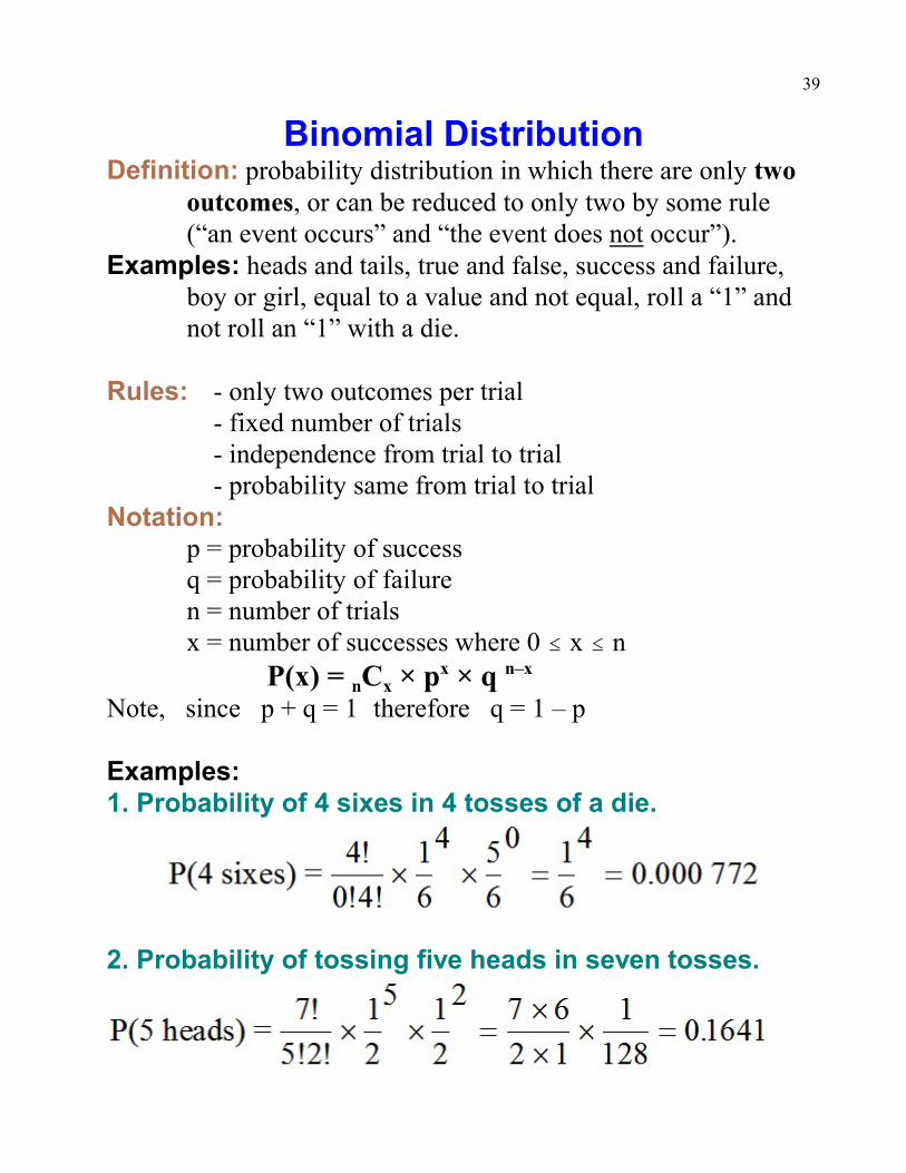
Binomial DistributionDefinition: probability distribution in which there are only two
outcomes, or can be reduced to only two by some rule(“an event occurs” and “the event does not occur”).
Examples: heads and tails, true and false, success and failure,boy or girl, equal to a value and not equal, roll a “1” andnot roll an “1” with a die.
Rules: - only two outcomes per trial- fixed number of trials- independence from trial to trial- probability same from trial to trial
Notation:p = probability of successq = probability of failuren = number of trialsx = number of successes where 0 # x # n
n xP(x) = C × p × q x n–x
Note, since p + q = 1 therefore q = 1 – p
Examples:1. Probability of 4 sixes in 4 tosses of a die.
2. Probability of tossing five heads in seven tosses.
40
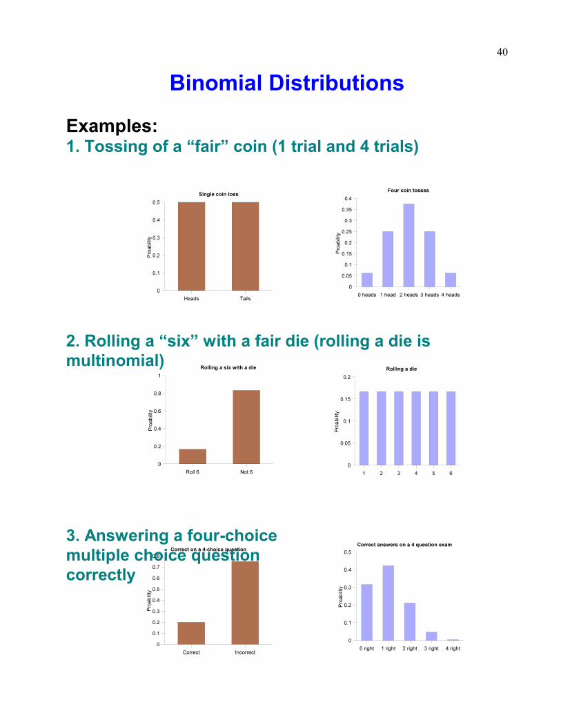
Binomial Distributions
Examples:1. Tossing of a “fair” coin (1 trial and 4 trials)
2. Rolling a “six” with a fair die (rolling a die ismultinomial)
3. Answering a four-choicemultiple choice questioncorrectly
41
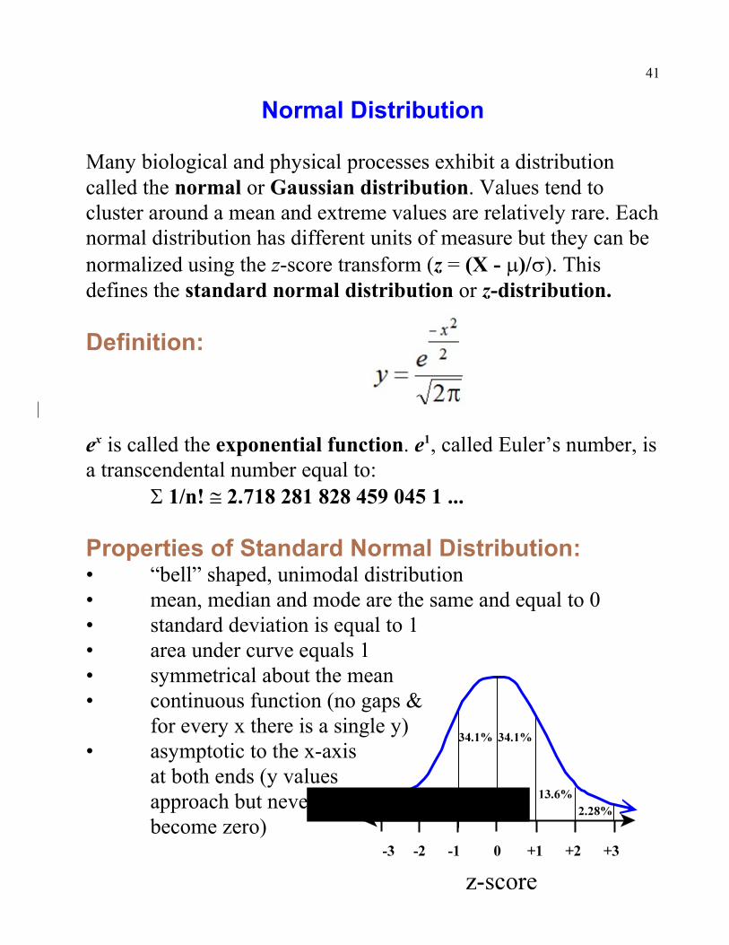
Normal Distribution
Many biological and physical processes exhibit a distributioncalled the normal or Gaussian distribution. Values tend tocluster around a mean and extreme values are relatively rare. Eachnormal distribution has different units of measure but they can benormalized using the z-score transform (z = (X - m)/s). Thisdefines the standard normal distribution or z-distribution.
Definition:
e is called the exponential function. e , called Euler’s number, isx 1
a transcendental number equal to:S 1/n! @ 2.718 281 828 459 045 1 ...
Properties of Standard Normal Distribution: • “bell” shaped, unimodal distribution• mean, median and mode are the same and equal to 0• standard deviation is equal to 1• area under curve equals 1• symmetrical about the mean• continuous function (no gaps &
for every x there is a single y)• asymptotic to the x-axis at both ends (y values
approach but never become zero)
42
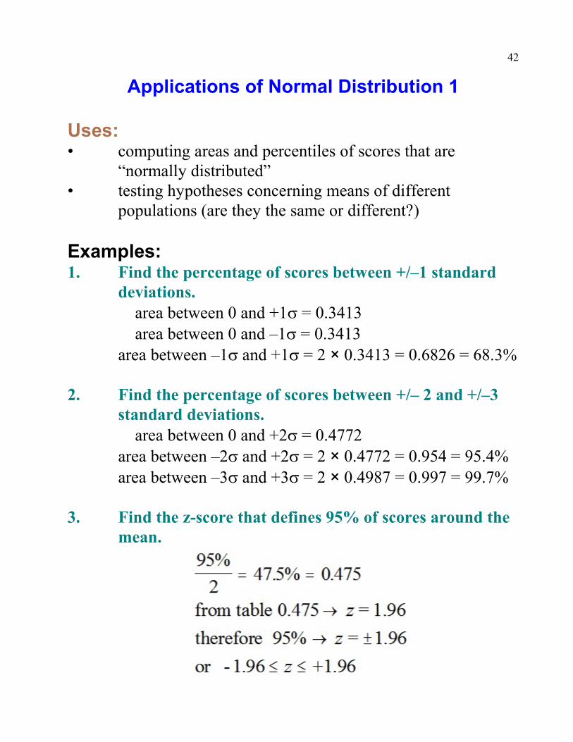
Applications of Normal Distribution 1
Uses: • computing areas and percentiles of scores that are
“normally distributed”• testing hypotheses concerning means of different
populations (are they the same or different?)
Examples:1. Find the percentage of scores between +/–1 standard
deviations.area between 0 and +1s = 0.3413area between 0 and –1s = 0.3413
area between –1s and +1s = 2 × 0.3413 = 0.6826 = 68.3%
2. Find the percentage of scores between +/– 2 and +/–3standard deviations.
area between 0 and +2s = 0.4772area between –2s and +2s = 2 × 0.4772 = 0.954 = 95.4%area between –3s and +3s = 2 × 0.4987 = 0.997 = 99.7%
3. Find the z-score that defines 95% of scores around themean.
43
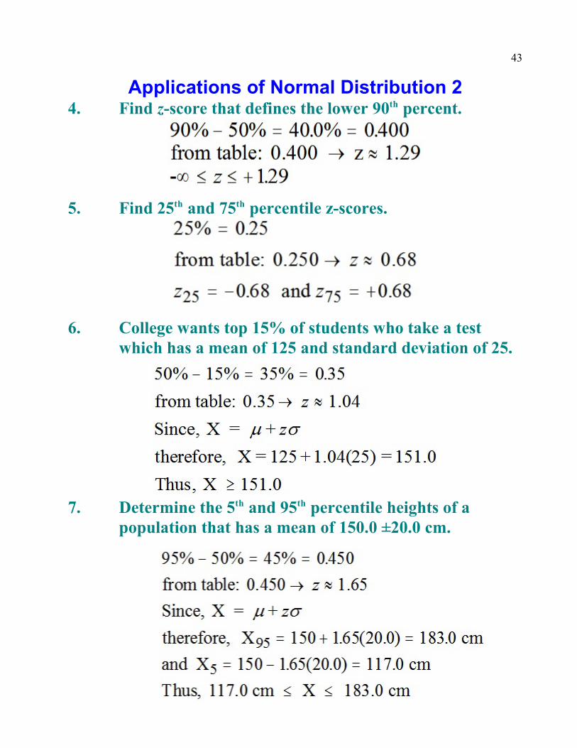
Applications of Normal Distribution 24. Find z-score that defines the lower 90 percent.th
5. Find 25 and 75 percentile z-scores.th th
6. College wants top 15% of students who take a testwhich has a mean of 125 and standard deviation of 25.
7. Determine the 5 and 95 percentile heights of ath th
population that has a mean of 150.0 ±20.0 cm.
44
Central Limit Theorem 1
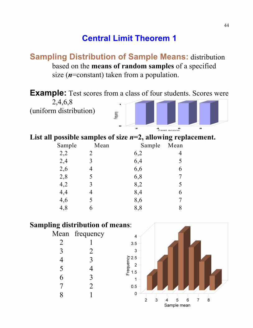
Sampling Distribution of Sample Means: distributionbased on the means of random samples of a specifiedsize (n=constant) taken from a population.
Example: Test scores from a class of four students. Scores were2,4,6,8
(uniform distribution)
List all possible samples of size n=2, allowing replacement. Sample Mean Sample Mean
2,2 2 6,2 4
2,4 3 6,4 5
2,6 4 6,6 6
2,8 5 6,8 7
4,2 3 8,2 5
4,4 4 8,4 6
4,6 5 8,6 7
4,8 6 8,8 8
Sampling distribution of means:Mean frequency
2 13 24 35 46 37 28 1
45
Central Limit Theorem 2
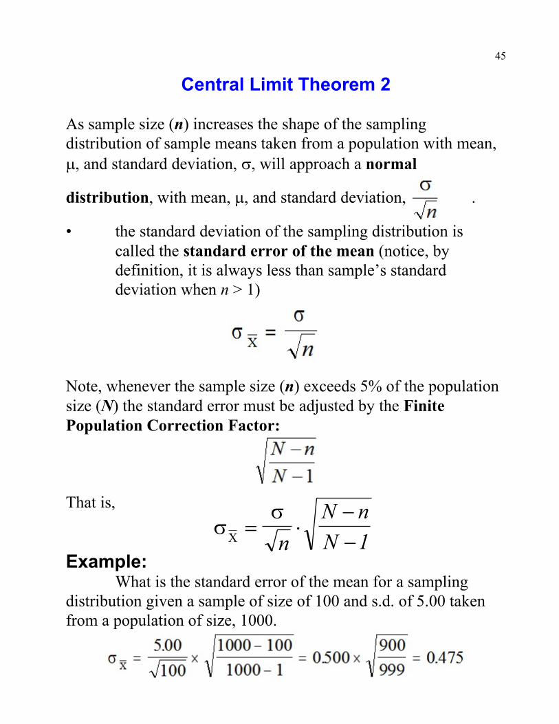
As sample size (n) increases the shape of the samplingdistribution of sample means taken from a population with mean,m, and standard deviation, s, will approach a normal
distribution, with mean, m, and standard deviation, .
• the standard deviation of the sampling distribution iscalled the standard error of the mean (notice, bydefinition, it is always less than sample’s standarddeviation when n > 1)
Note, whenever the sample size (n) exceeds 5% of the populationsize (N) the standard error must be adjusted by the FinitePopulation Correction Factor:
That is,
Example:What is the standard error of the mean for a sampling
distribution given a sample of size of 100 and s.d. of 5.00 takenfrom a population of size, 1000.
46
Confidence Intervals 1
Point Estimate:• a specific value that estimates a parameter
• e.g., a sample mean ( ) is “best estimator” of thepopulation mean (m)
• problem is that there is no way to determine how close apoint estimate is to the parameter
Properties of a Good Estimator:1. must be an unbiased estimator -expected value of
estimator or mean obtained from samples of a given sizemust be equal to the parameter
2. must be consistent -as sample size increases estimatorapproaches value of the parameter
3. must be relatively efficient -estimator must havesmallest variance of all other estimators
Interval Estimate:• range of values that estimate a parameter• e.g., mean +/- standard deviation (s), 25 ± 10 kg, 5 toth
95 %ileth
• precise probabilities can be assigned the validity of theinterval
47
Confidence Intervals 2
Confidence Interval:• interval estimate based on sample data and a given
confidence level
Confidence Level:• probability that a parameter will fall within an interval
estimate• related to alpha (a) level, that is,
Confidence Level = 1 - aE.g., C.L. = 95% means a = 0.05
C.L. = 99% means a = 0.01
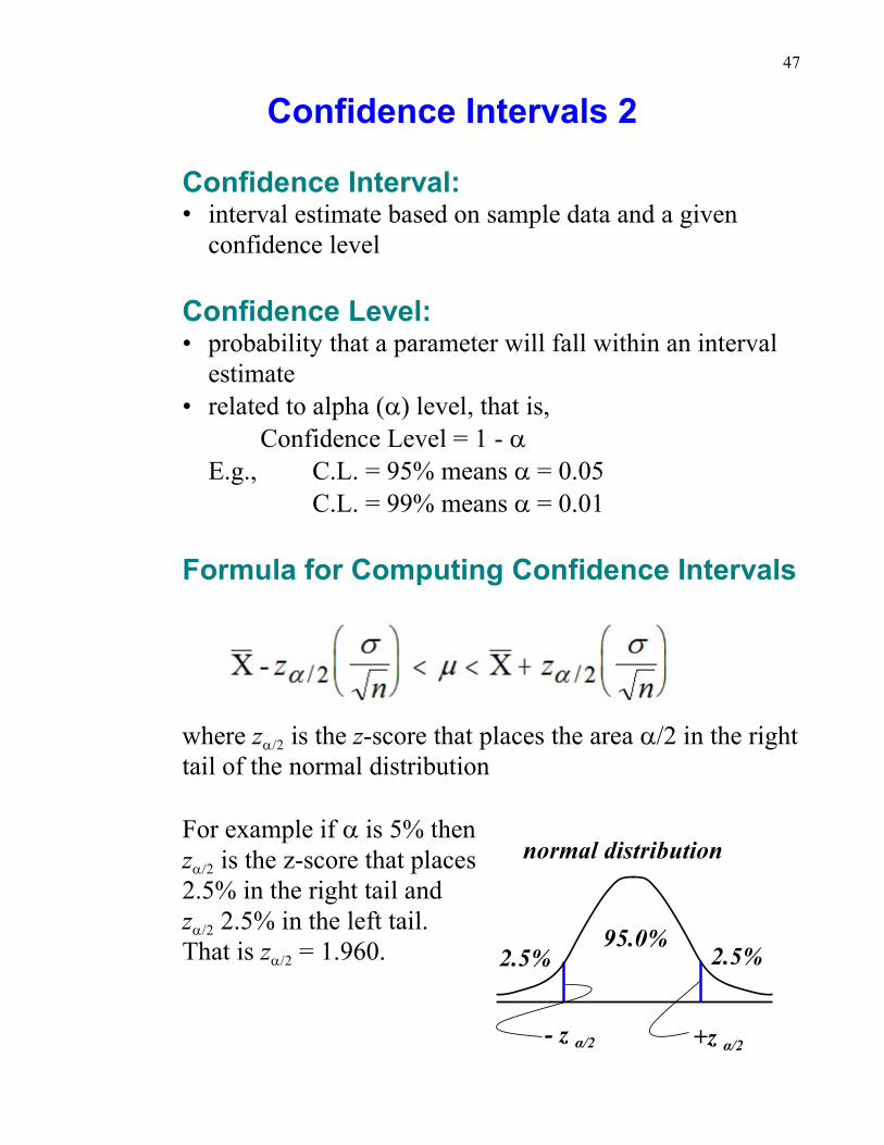
Formula for Computing Confidence Intervals
a/2where z is the z-score that places the area a/2 in the righttail of the normal distribution
For example if a is 5% then
a/2z is the z-score that places2.5% in the right tail and
a/2z 2.5% in the left tail.
a/2That is z = 1.960.
48
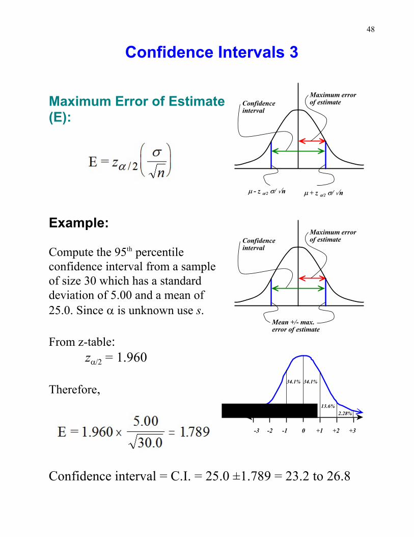
Confidence Intervals 3
Maximum Error of Estimate(E):
Example:
Compute the 95 percentileth
confidence interval from a sampleof size 30 which has a standarddeviation of 5.00 and a mean of25.0. Since a is unknown use s.
From z-table:
a/2z = 1.960
Therefore,
Confidence interval = C.I. = 25.0 ±1.789 = 23.2 to 26.8
49
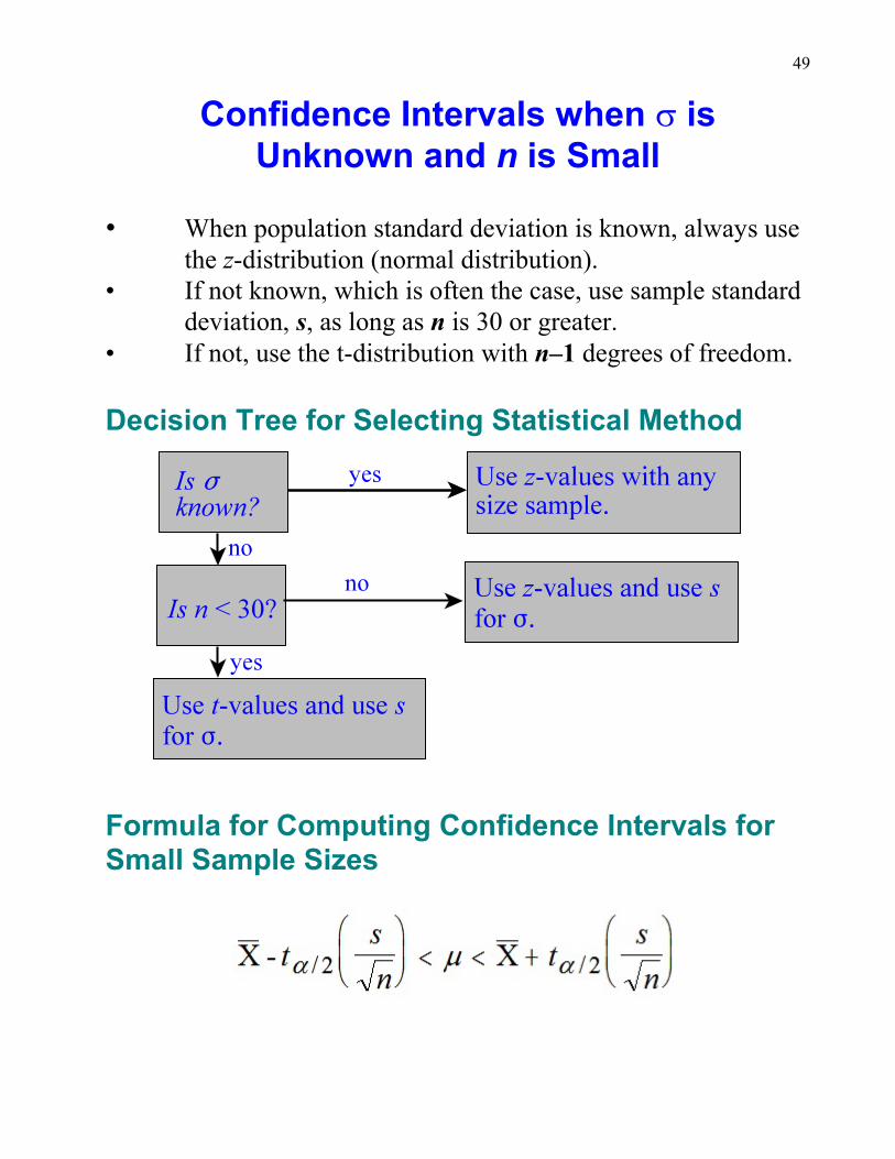
Confidence Intervals when s isUnknown and n is Small
• When population standard deviation is known, always usethe z-distribution (normal distribution).
• If not known, which is often the case, use sample standarddeviation, s, as long as n is 30 or greater.
• If not, use the t-distribution with n–1 degrees of freedom.
Decision Tree for Selecting Statistical Method
Formula for Computing Confidence Intervals forSmall Sample Sizes
50
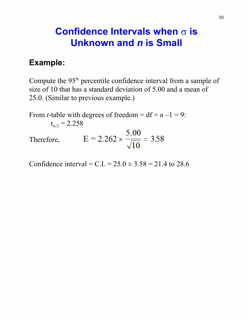
Confidence Intervals when s isUnknown and n is Small
Example:
Compute the 95 percentile confidence interval from a sample ofth
size of 10 that has a standard deviation of 5.00 and a mean of25.0. (Similar to previous example.)
From t-table with degrees of freedom = df = n –1 = 9:
a/2t = 2.258
Therefore,
Confidence interval = C.I. = 25.0 ± 3.58 = 21.4 to 28.6
51
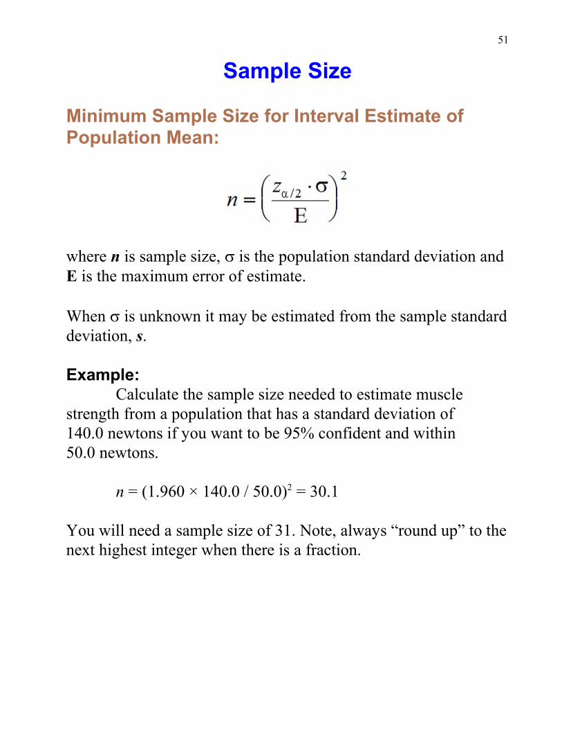
Sample Size
Minimum Sample Size for Interval Estimate ofPopulation Mean:
where n is sample size, s is the population standard deviation andE is the maximum error of estimate.
When s is unknown it may be estimated from the sample standarddeviation, s.
Example:Calculate the sample size needed to estimate muscle
strength from a population that has a standard deviation of140.0 newtons if you want to be 95% confident and within50.0 newtons.
n = (1.960 × 140.0 / 50.0) = 30.12
You will need a sample size of 31. Note, always “round up” to thenext highest integer when there is a fraction.
52
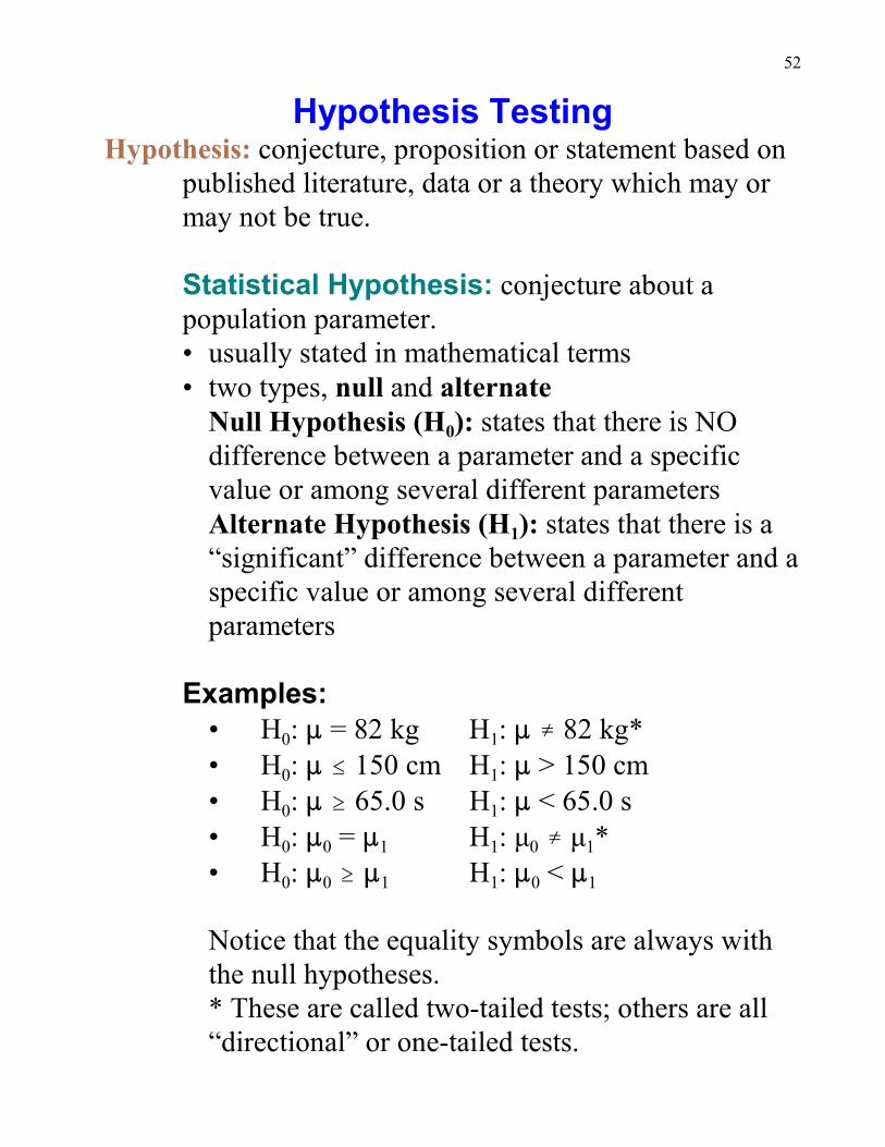
Hypothesis TestingHypothesis: conjecture, proposition or statement based on
published literature, data or a theory which may ormay not be true.
Statistical Hypothesis: conjecture about apopulation parameter.• usually stated in mathematical terms• two types, null and alternate
0Null Hypothesis (H ): states that there is NOdifference between a parameter and a specificvalue or among several different parameters
1Alternate Hypothesis (H ): states that there is a“significant” difference between a parameter and aspecific value or among several differentparameters
Examples:
0 1• H : : = 82 kg H : : � 82 kg*
0 1• H : : # 150 cm H : : > 150 cm
0 1• H : : $ 65.0 s H : : < 65.0 s
0 0 1 1 0 1• H : : = : H : ì � ì *
0 0 1 1 0 1• H : : $ : H : : < :
Notice that the equality symbols are always withthe null hypotheses.* These are called two-tailed tests; others are all“directional” or one-tailed tests.
53
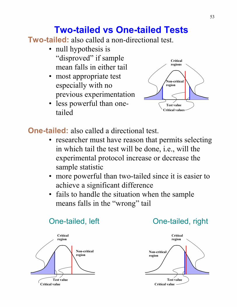
Two-tailed vs One-tailed TestsTwo-tailed: also called a non-directional test.
• null hypothesis is“disproved” if samplemean falls in either tail
• most appropriate testespecially with noprevious experimentation
• less powerful than one-tailed
One-tailed: also called a directional test.• researcher must have reason that permits selecting
in which tail the test will be done, i.e., will theexperimental protocol increase or decrease thesample statistic
• more powerful than two-tailed since it is easier toachieve a significant difference
• fails to handle the situation when the samplemeans falls in the “wrong” tail
One-tailed, left One-tailed, right
54
Statistical Testing
To determine the veracity (truth) of an hypothesis a statisticaltest must be undertaken that yields a test value. This value is thenevaluated to determine if it falls in the critical region of aappropriate probability distribution for a given significance oralpha (a) level.
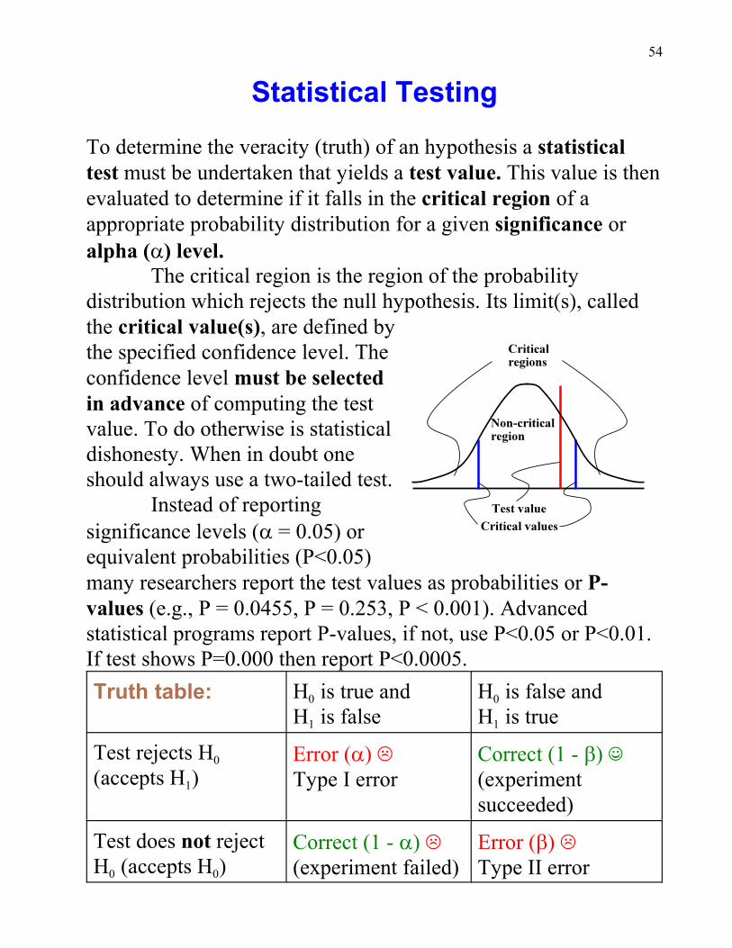
The critical region is the region of the probabilitydistribution which rejects the null hypothesis. Its limit(s), calledthe critical value(s), are defined bythe specified confidence level. Theconfidence level must be selectedin advance of computing the testvalue. To do otherwise is statisticaldishonesty. When in doubt oneshould always use a two-tailed test.
Instead of reportingsignificance levels (a = 0.05) orequivalent probabilities (P<0.05)many researchers report the test values as probabilities or P-values (e.g., P = 0.0455, P = 0.253, P < 0.001). Advancedstatistical programs report P-values, if not, use P<0.05 or P<0.01. If test shows P=0.000 then report P<0.0005.
Truth table: 0H is true and
1H is false0H is false and
1H is true
0Test rejects H
1(accepts H )Error (a) ;Type I error
Correct (1 - b) ((experimentsucceeded)
Test does not reject
0 0H (accepts H )Correct (1 - a) ;(experiment failed)
Error (b) ;Type II error
55
z-Test and t-Test
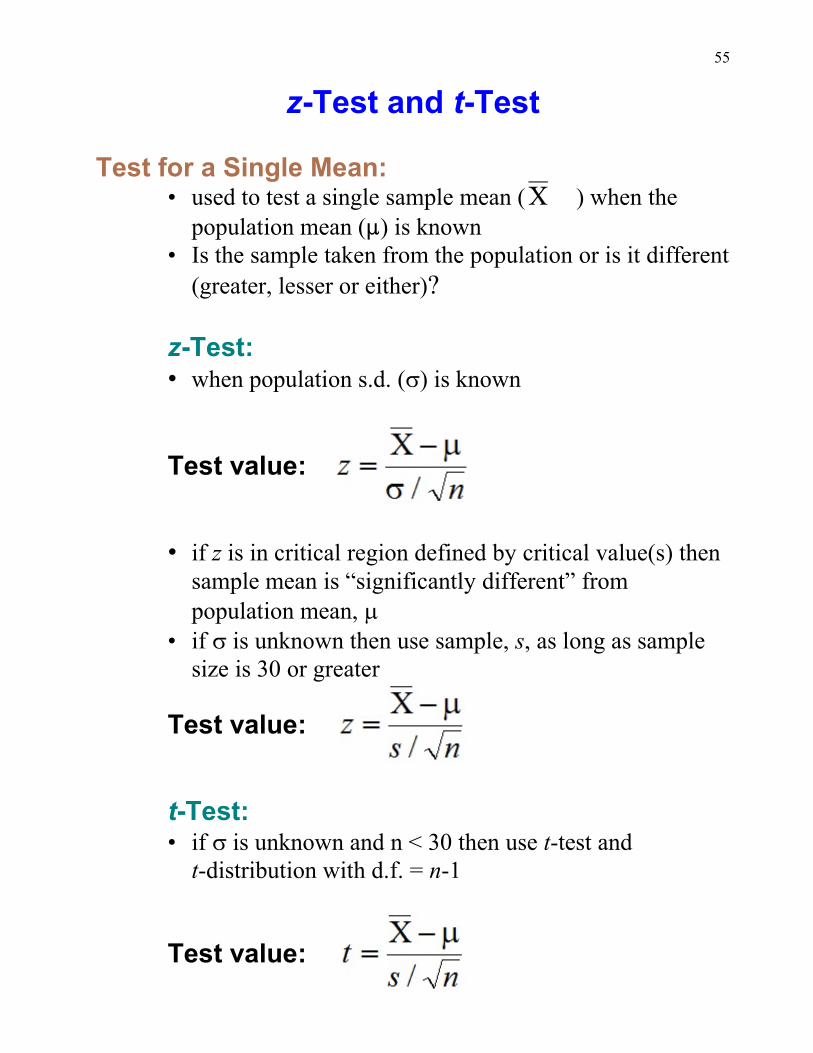
Test for a Single Mean: • used to test a single sample mean ( ) when the
population mean (:) is known• Is the sample taken from the population or is it different
(greater, lesser or either)?
z-Test:• when population s.d. (s) is known
Test value:
• if z is in critical region defined by critical value(s) thensample mean is “significantly different” frompopulation mean, m
• if s is unknown then use sample, s, as long as samplesize is 30 or greater
Test value:
t-Test:• if s is unknown and n < 30 then use t-test and
t-distribution with d.f. = n-1
Test value:
56
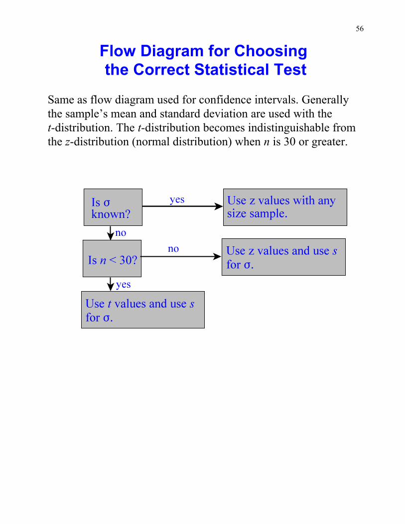
Flow Diagram for Choosing the Correct Statistical Test
Same as flow diagram used for confidence intervals. Generallythe sample’s mean and standard deviation are used with thet-distribution. The t-distribution becomes indistinguishable fromthe z-distribution (normal distribution) when n is 30 or greater.
57
Power of a Statistical Test
Power: ability of a statistical test to detect a real difference.• probability of rejecting the null hypothesis when it is
false (i.e., there is a real difference)• equal to 1 – b (1 – probability of Type II error)
Ways of increasing power
• Increasing a will increase power but it also increaseschance of a Type I error
• Increasing sample size (increases costs)• Using ratio or interval data versus nominal or ordinal.
Tests involving ratio/interval data are called“parametric” tests. Those involving nominal andordinal data are called “nonparametric” tests.
• Using “repeated measures” tests, such as, therepeated measures t-test or ANOVA. By using the samesubjects repeatedly, variability is reduced.
• If variances are equal use pooled estimates of variance(e.g., Independent groups t-test)
• Using samples that represent extremes. Reducesgeneralizability of experiment results.
• Standardizing testing procedures reduces variability.• Using one-tailed vs. two-tailed tests. Problem occurs if
results are in wrong tail. Not recommended.
58
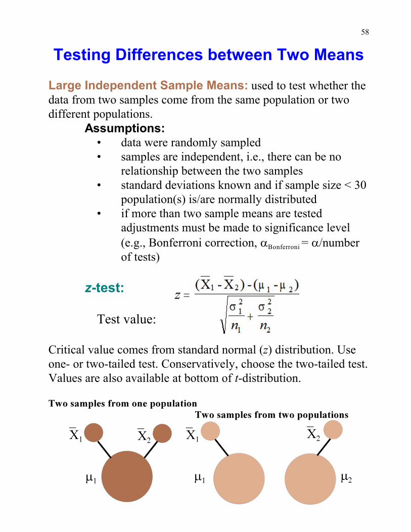
Testing Differences between Two Means
Large Independent Sample Means: used to test whether thedata from two samples come from the same population or twodifferent populations.
Assumptions:• data were randomly sampled• samples are independent, i.e., there can be no
relationship between the two samples• standard deviations known and if sample size < 30
population(s) is/are normally distributed• if more than two sample means are tested
adjustments must be made to significance level
Bonferroni (e.g., Bonferroni correction, a = a/numberof tests)
z-test:
Test value:
Critical value comes from standard normal (z) distribution. Useone- or two-tailed test. Conservatively, choose the two-tailed test.Values are also available at bottom of t-distribution.
59
The Step-by-Step Approach
Step 1: State hypothesesTwo-tailed: One-tailed:
0 1 2 0 1 2 0 1 2H : : = : H : : # : or H : : $ :
1 1 2 1 1 2 1 1 2H : : � : H : : > : or H : : < :
Step 2: Find critical valueLook up z-score for specified significance (a) level and forone- or two-tailed test (selected in advance). Usually use
criticala = 0.05 and two-tailed test, i.e., z = ±1.960. For one-
criticaltailed use z = ±1.645.
Step 3: Compute testvalue
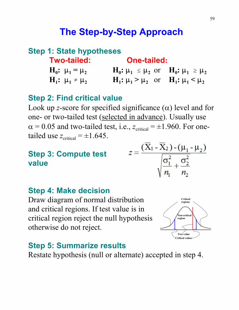
Step 4: Make decisionDraw diagram of normal distributionand critical regions. If test value is incritical region reject the null hypothesisotherwise do not reject.
Step 5: Summarize resultsRestate hypothesis (null or alternate) accepted in step 4.
60
If null is rejected:There is enough evidence to reject the null
hypothesis.
If null is not rejected:There is not enough evidence to reject the null
hypothesis.
Optionally, reword hypothesis in “lay” terms. E.g., Thereis or is not a difference between the two populations orone population is greater/lesser than the other for theindependent variable.
61
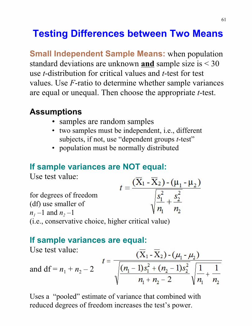
Testing Differences between Two Means
Small Independent Sample Means: when populationstandard deviations are unknown and sample size is < 30use t-distribution for critical values and t-test for testvalues. Use F-ratio to determine whether sample variancesare equal or unequal. Then choose the appropriate t-test.
Assumptions• samples are random samples • two samples must be independent, i.e., different
subjects, if not, use “dependent groups t-test”• population must be normally distributed
If sample variances are NOT equal:Use test value:
for degrees of freedom(df) use smaller of
1 2n –1 and n –1(i.e., conservative choice, higher critical value)
If sample variances are equal:Use test value:
1 2and df = n + n – 2
Uses a “pooled” estimate of variance that combined withreduced degrees of freedom increases the test’s power.
62
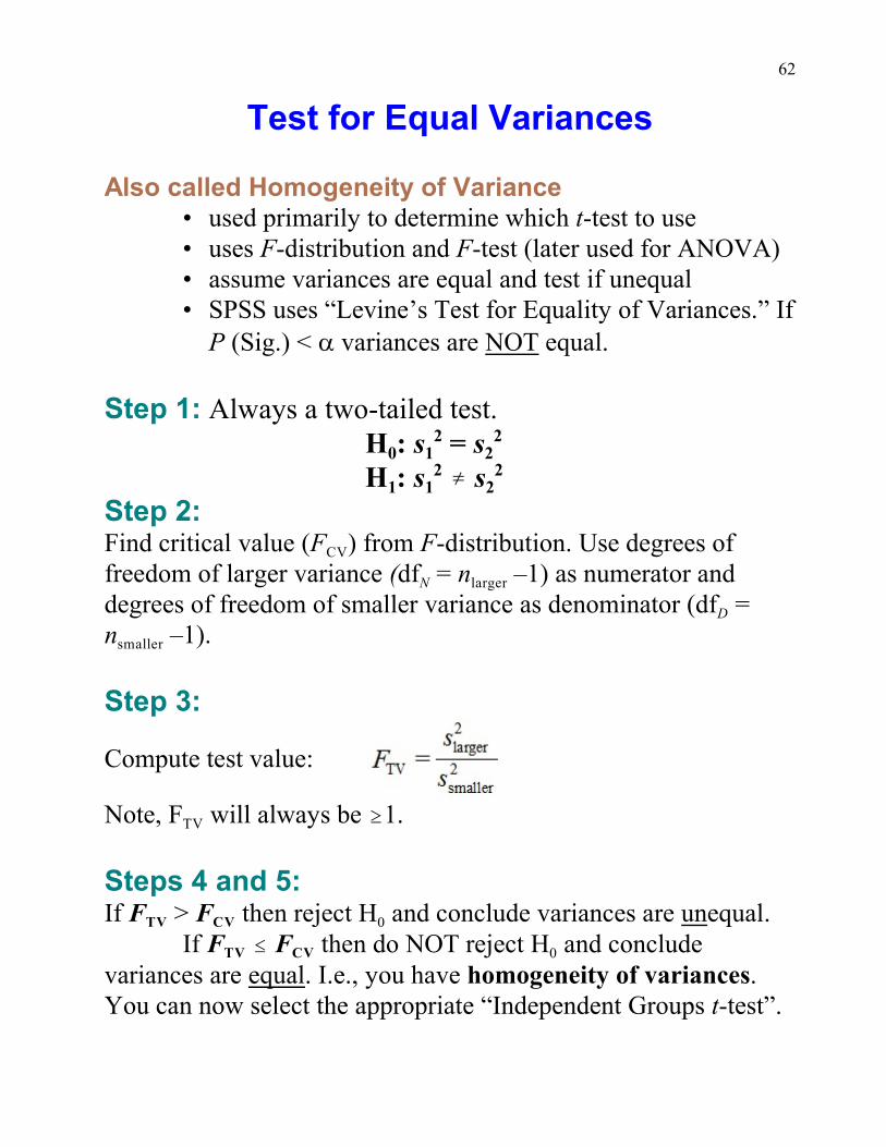
Test for Equal Variances
Also called Homogeneity of Variance• used primarily to determine which t-test to use• uses F-distribution and F-test (later used for ANOVA)• assume variances are equal and test if unequal• SPSS uses “Levine’s Test for Equality of Variances.” If
P (Sig.) < a variances are NOT equal.
Step 1: Always a two-tailed test.
0 1 2H : s = s2 2
1 1 2H : s � s2 2
Step 2:CVFind critical value (F ) from F-distribution. Use degrees of
N largerfreedom of larger variance (df = n –1) as numerator and
Ddegrees of freedom of smaller variance as denominator (df =
smallern –1).
Step 3:
Compute test value:
TVNote, F will always be $1.
Steps 4 and 5:
0TV CVIf F > F then reject H and conclude variances are unequal.
0TV CVIf F # F then do NOT reject H and concludevariances are equal. I.e., you have homogeneity of variances.You can now select the appropriate “Independent Groups t-test”.
63
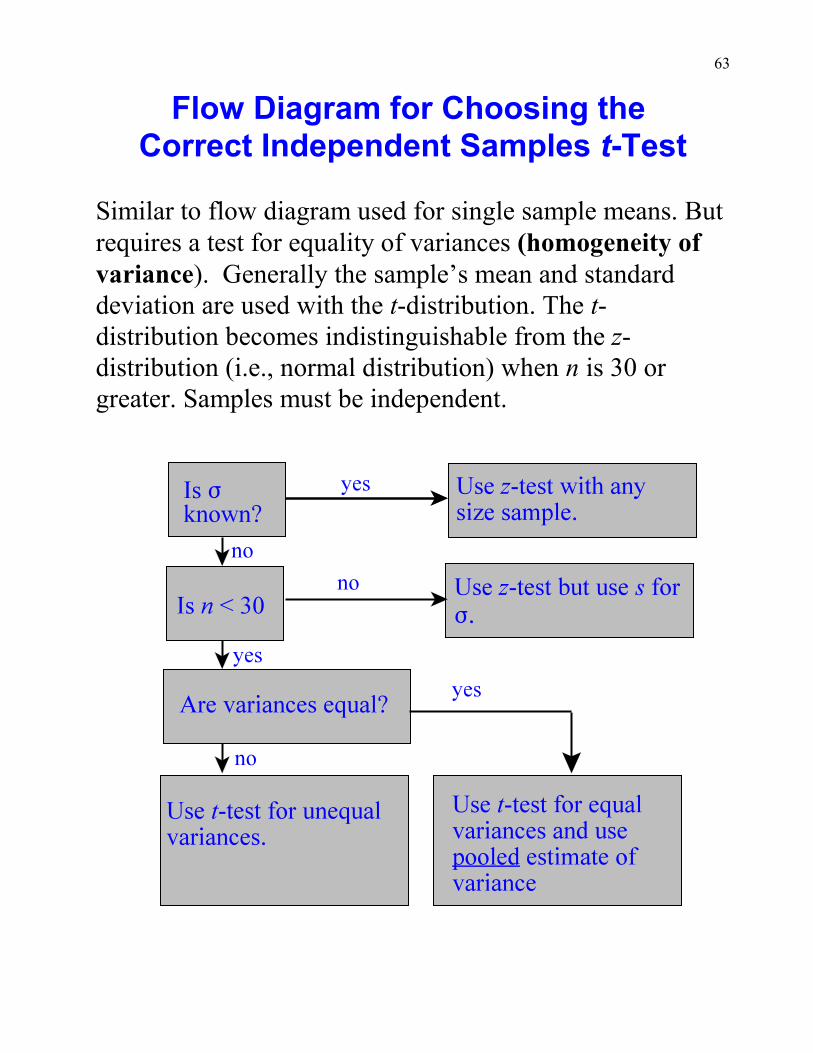
Flow Diagram for Choosing the Correct Independent Samples t-Test
Similar to flow diagram used for single sample means. Butrequires a test for equality of variances (homogeneity ofvariance). Generally the sample’s mean and standarddeviation are used with the t-distribution. The t-distribution becomes indistinguishable from the z-distribution (i.e., normal distribution) when n is 30 orgreater. Samples must be independent.
64
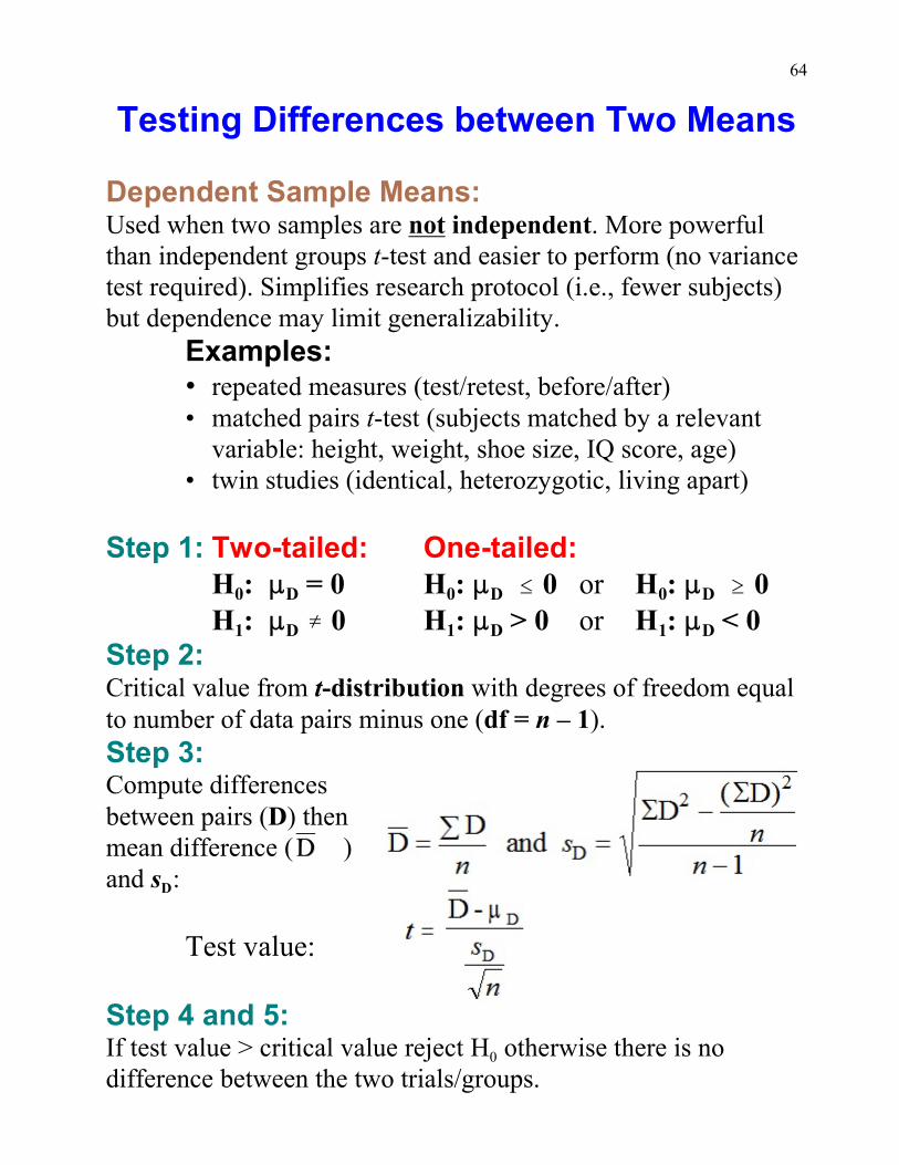
Testing Differences between Two Means
Dependent Sample Means:Used when two samples are not independent. More powerfulthan independent groups t-test and easier to perform (no variancetest required). Simplifies research protocol (i.e., fewer subjects)but dependence may limit generalizability.
Examples:• repeated measures (test/retest, before/after)• matched pairs t-test (subjects matched by a relevant
variable: height, weight, shoe size, IQ score, age)• twin studies (identical, heterozygotic, living apart)
Step 1: Two-tailed: One-tailed:
0 D 0 D 0 DH : : = 0 H : : # 0 or H : : $ 0
1 D 1 D 1 DH : : � 0 H : : > 0 or H : : < 0Step 2:Critical value from t-distribution with degrees of freedom equalto number of data pairs minus one (df = n – 1).
Step 3:Compute differencesbetween pairs (D) thenmean difference ( )
Dand s :
Test value:
Step 4 and 5:0If test value > critical value reject H otherwise there is no
difference between the two trials/groups.
65
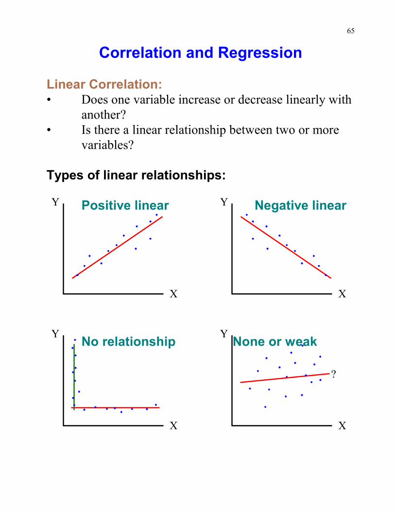
Correlation and Regression
Linear Correlation:• Does one variable increase or decrease linearly with
another?• Is there a linear relationship between two or more
variables?
Types of linear relationships:
Positive linear Negative linear
No relationship None or weak
66
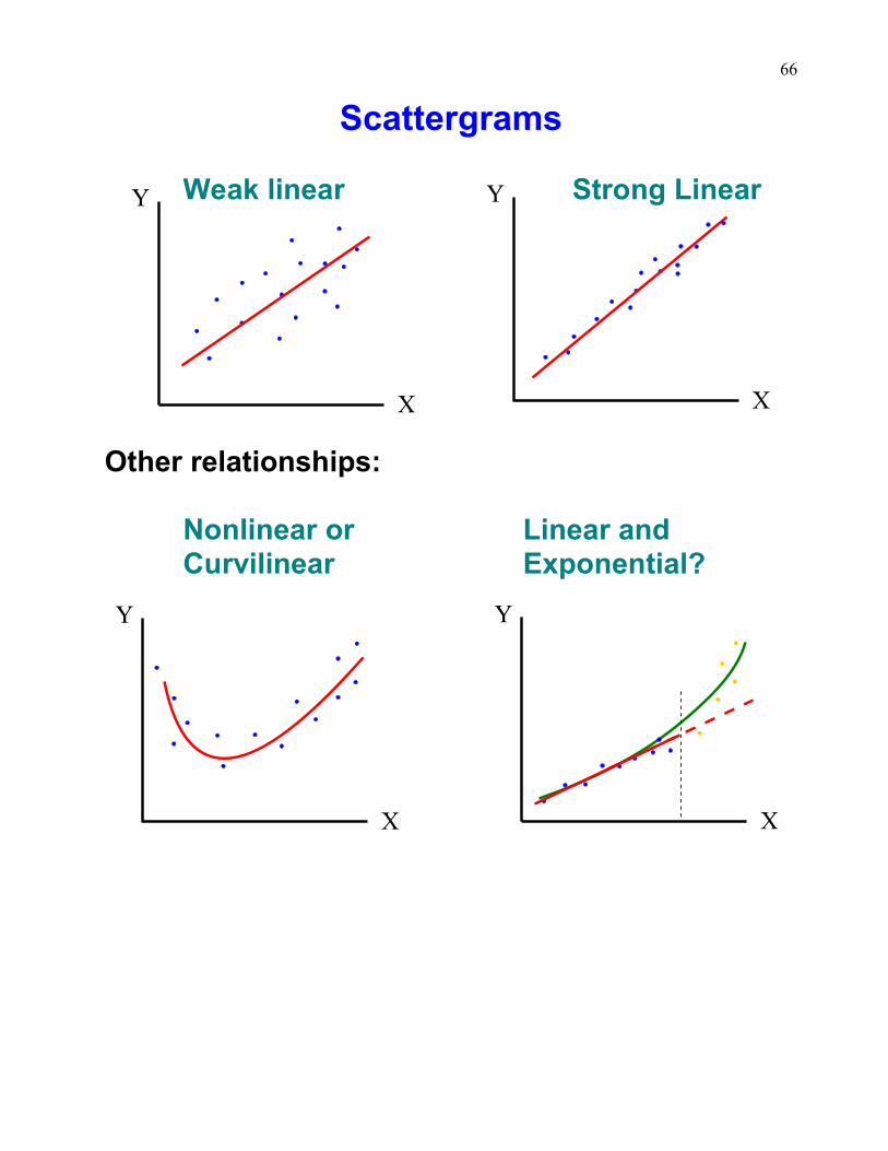
Scattergrams
Weak linear Strong Linear
Other relationships:
Nonlinear or Linear andCurvilinear Exponential?
67
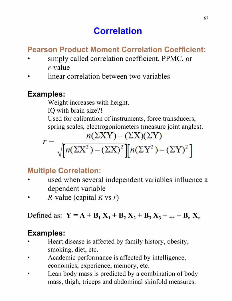
Correlation
Pearson Product Moment Correlation Coefficient:• simply called correlation coefficient, PPMC, or
r-value• linear correlation between two variables
Examples:Weight increases with height.IQ with brain size?!Used for calibration of instruments, force transducers,spring scales, electrogoniometers (measure joint angles).
Multiple Correlation:• used when several independent variables influence a
dependent variable• R-value (capital R vs r)
1 1 2 2 3 3 n nDefined as: Y = A + B X + B X + B X + ... + B X
Examples:• Heart disease is affected by family history, obesity,
smoking, diet, etc.• Academic performance is affected by intelligence,
economics, experience, memory, etc.• Lean body mass is predicted by a combination of body
mass, thigh, triceps and abdominal skinfold measures.
68
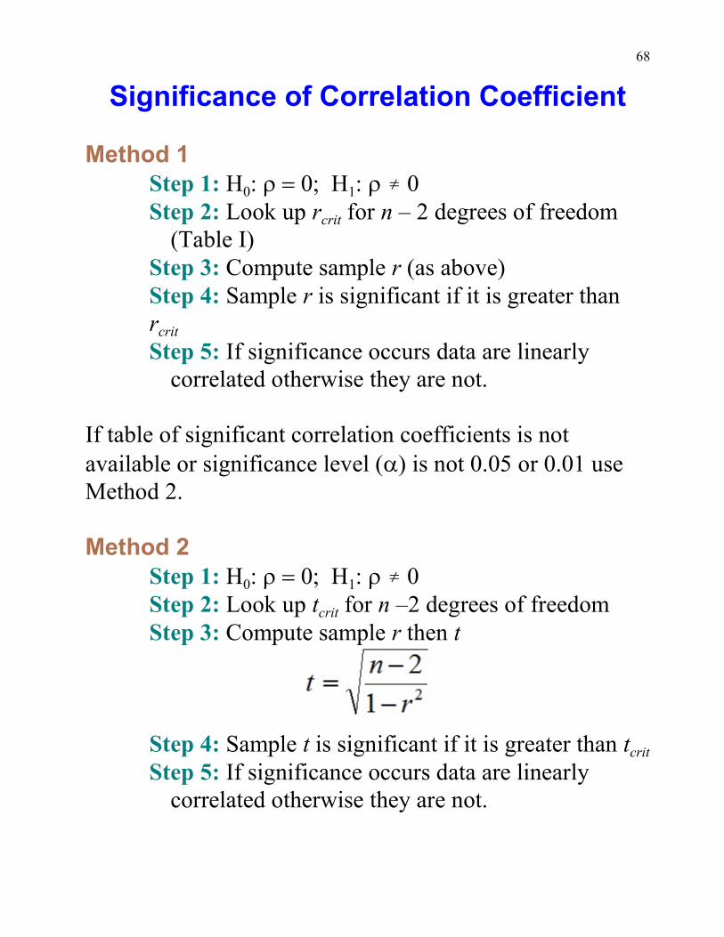
Significance of Correlation Coefficient
Method 1Step 1: 0 1 H : r = 0; H : r � 0Step 2: crit Look up r for n – 2 degrees of freedom
(Table I)Step 3: Compute sample r (as above)Step 4: Sample r is significant if it is greater than
critr Step 5: If significance occurs data are linearly
correlated otherwise they are not.
If table of significant correlation coefficients is notavailable or significance level (a) is not 0.05 or 0.01 useMethod 2.
Method 2Step 1: 0 1 H : r = 0; H : r � 0Step 2: crit Look up t for n –2 degrees of freedom Step 3: Compute sample r then t
Step 4: crit Sample t is significant if it is greater than t Step 5: If significance occurs data are linearly
correlated otherwise they are not.
69
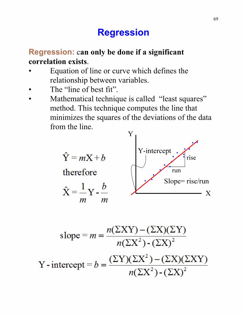
Regression
Regression: can only be done if a significantcorrelation exists.• Equation of line or curve which defines the
relationship between variables.• The “line of best fit”.• Mathematical technique is called “least squares”
method. This technique computes the line thatminimizes the squares of the deviations of the datafrom the line.
70
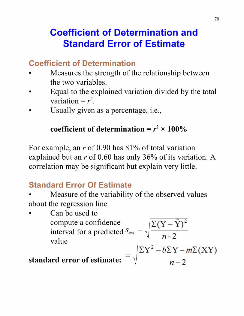
Coefficient of Determination andStandard Error of Estimate
Coefficient of Determination• Measures the strength of the relationship between
the two variables.• Equal to the explained variation divided by the total
variation = r .2
• Usually given as a percentage, i.e.,
coefficient of determination = r × 100%2
For example, an r of 0.90 has 81% of total variationexplained but an r of 0.60 has only 36% of its variation. Acorrelation may be significant but explain very little.
Standard Error Of Estimate• Measure of the variability of the observed valuesabout the regression line• Can be used to
compute a confidenceinterval for a predictedvalue
standard error of estimate:
71
Possible Reasons for a Significant Correlation
1. There is a direct cause-and-effect relationship between thevariables. That is, x causes y. For example, positive reinforcementimproves learning, smoking causes lung cancer and heat causes ice tomelt.
2. There is a reverse cause-and-effect relationship between thevariables. That is, y causes x. For example, suppose a researcherbelieves excessive coffee consumption causes nervousness, but theresearcher fails to consider that the reverse situation may occur. That is,it may be that an nervous people crave coffee.
3. The relationship between the variables may be caused by athird variable. For example, if a statistician correlated the number ofdeaths due to drowning and the number of cans of soft drinksconsumed during the summer, he or she would probably find asignificant relationship. However, the soft drink is not necessarilyresponsible for the deaths, since both variables may be related to heatand humidity.
4. There may be a complexity of interrelationships among manyvariables. For example, a researcher may find a significant relationshipbetween students’ high school grades and college grades. But thereprobably are many other variables involved, such as IQ, hours of study,influence of parents, motivation, age and instructors.
5. The relationship may be coincidental. For example, aresearcher may be able to find a significant relationship between theincrease in the number of people who are exercising and the increase inthe number of people who are committing crimes. But common sensedictates that any relationship between these two variables must be dueto coincidence.
72
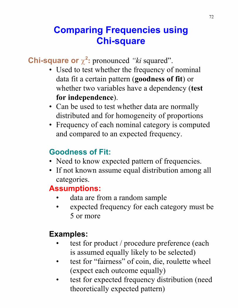
Comparing Frequencies usingChi-square
Chi-square or c :2 pronounced “ki squared”.• Used to test whether the frequency of nominal
data fit a certain pattern (goodness of fit) orwhether two variables have a dependency (testfor independence).
• Can be used to test whether data are normallydistributed and for homogeneity of proportions
• Frequency of each nominal category is computedand compared to an expected frequency.
Goodness of Fit:• Need to know expected pattern of frequencies.• If not known assume equal distribution among all
categories.Assumptions:
• data are from a random sample• expected frequency for each category must be
5 or more
Examples: • test for product / procedure preference (each
is assumed equally likely to be selected)• test for “fairness” of coin, die, roulette wheel
(expect each outcome equally)• test for expected frequency distribution (need
theoretically expected pattern)
73
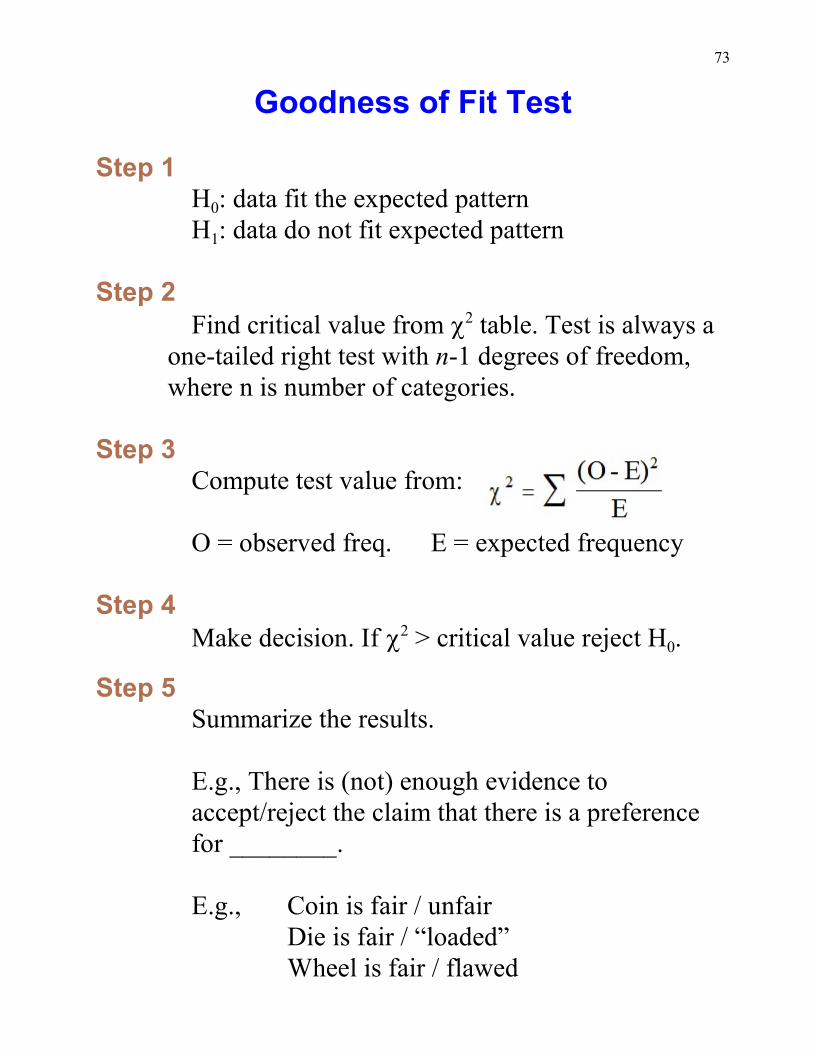
Goodness of Fit Test
Step 1
0H : data fit the expected pattern
1H : data do not fit expected pattern
Step 2Find critical value from c table. Test is always a2
one-tailed right test with n-1 degrees of freedom,where n is number of categories.
Step 3Compute test value from:
O = observed freq. E = expected frequency
Step 4
0Make decision. If c > critical value reject H .2
Step 5Summarize the results.
E.g., There is (not) enough evidence toaccept/reject the claim that there is a preferencefor ________.
E.g., Coin is fair / unfairDie is fair / “loaded”Wheel is fair / flawed
74
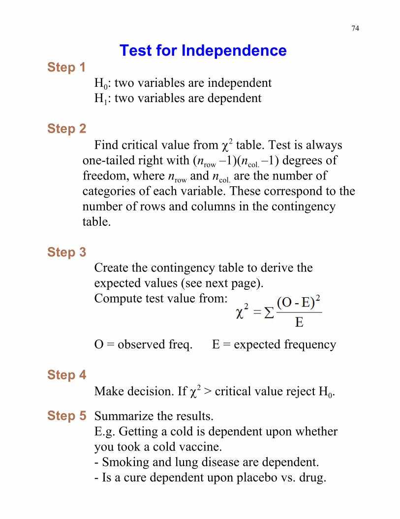
Test for IndependenceStep 1
0H : two variables are independent
1H : two variables are dependent
Step 2Find critical value from c table. Test is always2
row col. one-tailed right with (n –1)(n –1) degrees of
row col.freedom, where n and n are the number ofcategories of each variable. These correspond to thenumber of rows and columns in the contingencytable.
Step 3Create the contingency table to derive theexpected values (see next page).Compute test value from:
O = observed freq. E = expected frequency
Step 4
0Make decision. If c > critical value reject H .2
Step 5 Summarize the results.E.g. Getting a cold is dependent upon whetheryou took a cold vaccine.- Smoking and lung disease are dependent.- Is a cure dependent upon placebo vs. drug.
75
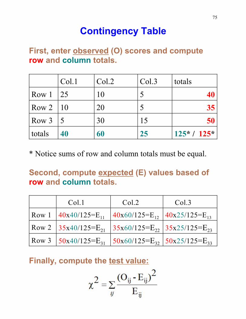
Contingency Table
First, enter observed (O) scores and computerow and column totals.
Col.1 Col.2 Col.3 totals
Row 1 25 10 5 40
Row 2 10 20 5 35
Row 3 5 30 15 50
totals 40 60 25 125* / 125*
* Notice sums of row and column totals must be equal.
Second, compute expected (E) values based ofrow and column totals.
Col.1 Col.2 Col.3
Row 1 40x40 11/125=E 40x60 12/125=E 40x25 13/125=E
Row 2 35x40 21/125=E 35x60 22/125=E 35x25 23/125=E
Row 3 50x40 31/125=E 50x60 32/125=E 50x25 33/125=E
Finally, compute the test value:
76
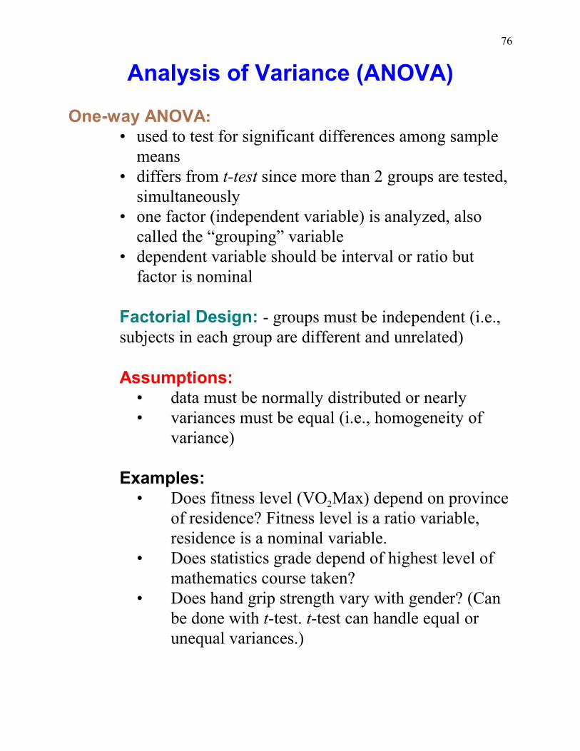
Analysis of Variance (ANOVA)
One-way ANOVA:• used to test for significant differences among sample
means • differs from t-test since more than 2 groups are tested,
simultaneously• one factor (independent variable) is analyzed, also
called the “grouping” variable• dependent variable should be interval or ratio but
factor is nominal
Factorial Design: - groups must be independent (i.e.,subjects in each group are different and unrelated)
Assumptions:• data must be normally distributed or nearly• variances must be equal (i.e., homogeneity of
variance)
Examples:
2• Does fitness level (VO Max) depend on provinceof residence? Fitness level is a ratio variable,residence is a nominal variable.
• Does statistics grade depend of highest level ofmathematics course taken?
• Does hand grip strength vary with gender? (Canbe done with t-test. t-test can handle equal orunequal variances.)
77
One-way ANOVA
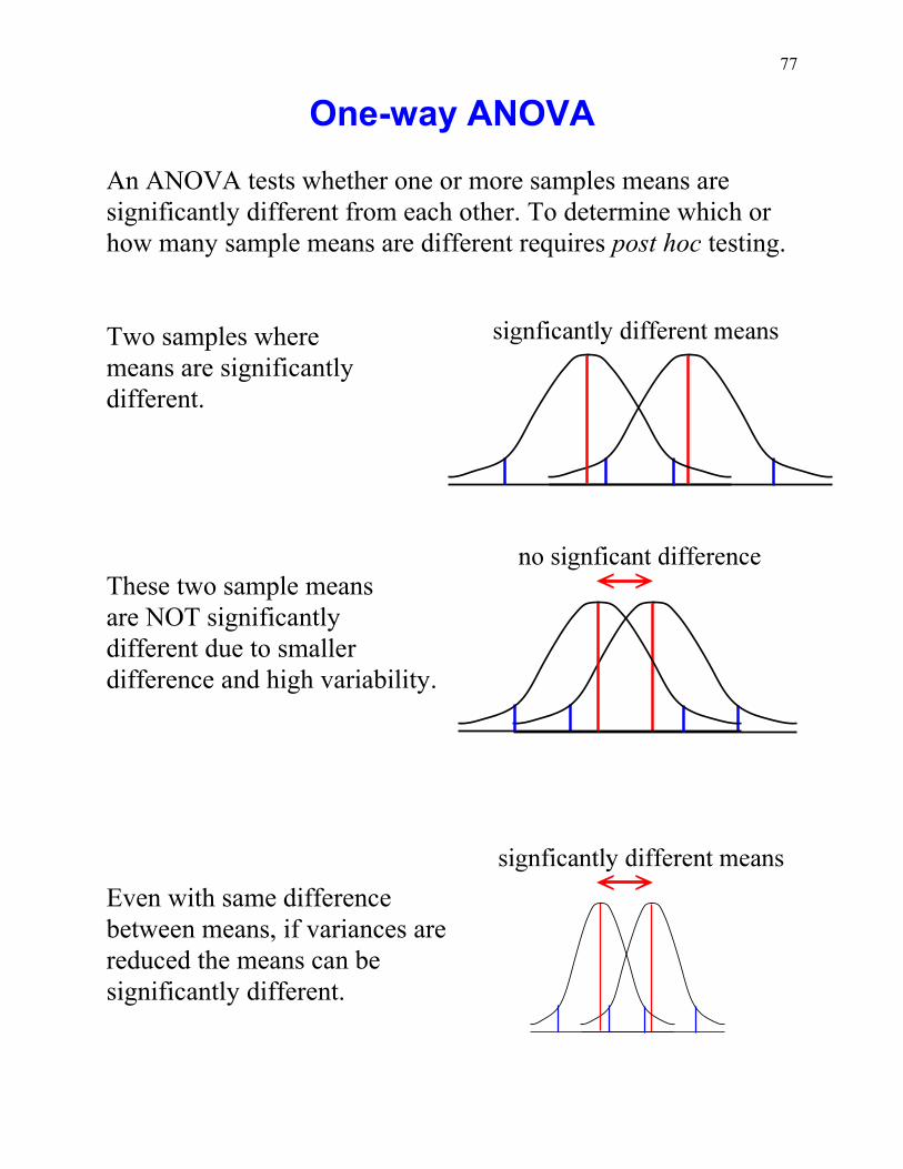
An ANOVA tests whether one or more samples means aresignificantly different from each other. To determine which orhow many sample means are different requires post hoc testing.
Two samples wheremeans are significantlydifferent.
These two sample meansare NOT significantlydifferent due to smallerdifference and high variability.
Even with same differencebetween means, if variances arereduced the means can besignificantly different.
78
One-way ANOVA
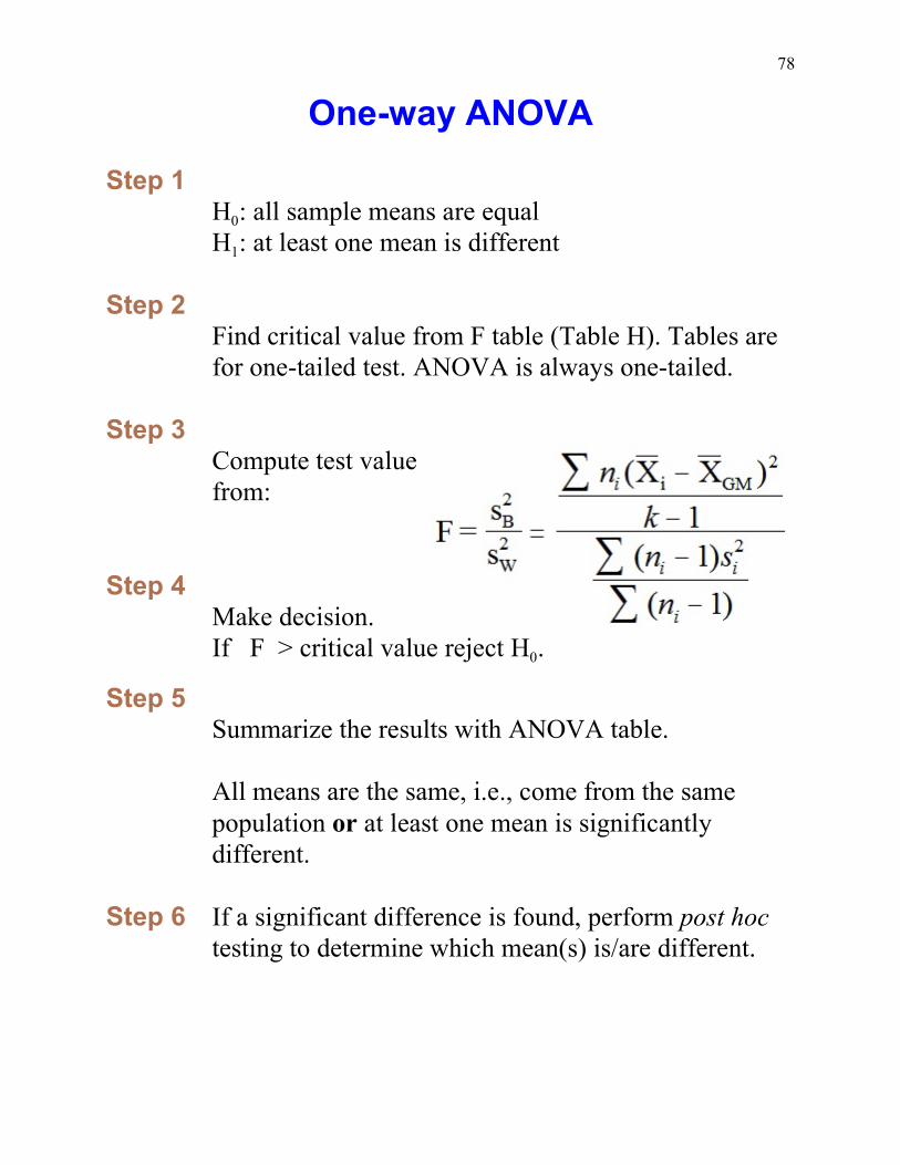
Step 1
0H : all sample means are equal
1H : at least one mean is different
Step 2Find critical value from F table (Table H). Tables arefor one-tailed test. ANOVA is always one-tailed.
Step 3Compute test valuefrom:
Step 4Make decision.
0If F > critical value reject H .
Step 5Summarize the results with ANOVA table.
All means are the same, i.e., come from the samepopulation or at least one mean is significantlydifferent.
Step 6 If a significant difference is found, perform post hoctesting to determine which mean(s) is/are different.
79
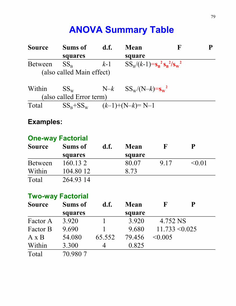
ANOVA Summary Table
Source Sums of d.f. Mean F Psquares square
B BBetween SS k-1 SS /(k-1) B B=s s2 2W/s 2
(also called Main effect)
W WWithin SS N–k SS /(N–k) W=s 2
(also called Error term)
B WTotal SS +SS (k–1)+(N–k)= N–1
Examples:
One-way FactorialSource Sums of d.f. Mean F P
squares squareBetween 160.13 2 80.07 9.17 <0.01Within 104.80 12 8.73Total 264.93 14
Two-way FactorialSource Sums of d.f. Mean F P
squares squareFactor A 3.920 1 3.920 4.752 NSFactor B 9.690 1 9.680 11.733 <0.025A x B 54.080 65.552 79.456 <0.005Within 3.300 4 0.825Total 70.980 7
80
Post Hoc Testing
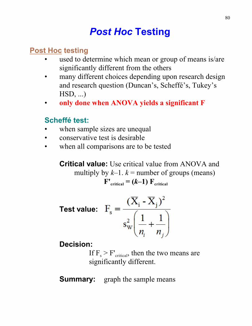
Post Hoc testing • used to determine which mean or group of means is/are
significantly different from the others• many different choices depending upon research design
and research question (Duncan’s, Scheffé’s, Tukey’sHSD, ...)
• only done when ANOVA yields a significant F
Scheffé test:• when sample sizes are unequal• conservative test is desirable• when all comparisons are to be tested
Critical value: Use critical value from ANOVA andmultiply by k–1. k = number of groups (means)
critical criticalF' = (k–1) F
Test value:
Decision:
s criticalIf F > F' , then the two means aresignificantly different.
Summary: graph the sample means
81
Post Hoc Testing 2
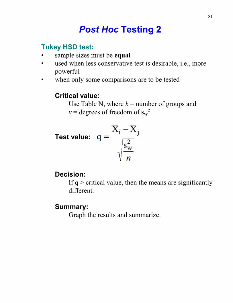
Tukey HSD test:• sample sizes must be equal• used when less conservative test is desirable, i.e., more
powerful• when only some comparisons are to be tested
Critical value:Use Table N, where k = number of groups and
Wv = degrees of freedom of s 2
Test value:
Decision:If q > critical value, then the means are significantlydifferent.
Summary:Graph the results and summarize.
82
Nonparametric Statistics
Nonparametric or Distribution-free statistics:• used when data are ordinal (i.e., rankings)• used when ratio/interval data are not normally
distributed (data are converted to ranks)• for studies not involving population parameters
Advantages:• no assumptions about distribution of data• suitable for ordinal data• can test hypotheses that do not involve population
parameters• computations are easier to perform• results are easier to understand
Disadvantages:• less powerful (less sensitive) than parametric• uses less information than parametric (ratio data are
reduced to ordinal scale)• less efficient, therefore larger sample sizes are needed to
detect significance
Examples: • Is there a bias in the rankings of judges from
different countries?• Is there a correlation between the rankings of two
judges?• Do different groups rank a professor’s teaching
differently?
83
Paired Sign Test
• used for repeated measures tests
Step 1
0H : no change/increase/decrease between before andafter tests
1H : there was a change/increase/decrease
Step 2Find critical value from table (Table J) for given a level,sample size (>7) and whether one- or two-tailedhypothesis
Step 3Subtract “after” from “before” scores, then count numberof positive (+) AND negative (–) differences. Zeros(pairs are equal) do not count.
Step 4Make decision. If smallest count (+ or –) less than
0critical value, reject H .
Step 5Summarize the result.
I.e., there was/was not a change or there was/was not andincrease/decrease in the dependent variable.
84
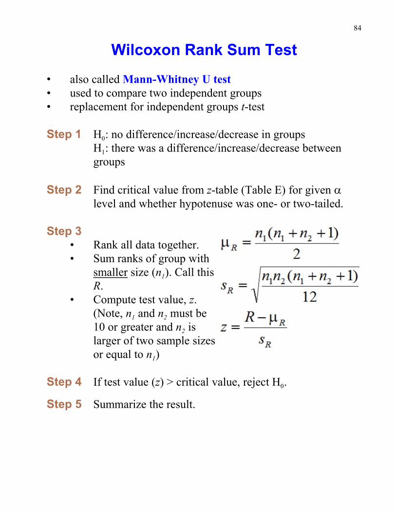
Wilcoxon Rank Sum Test
• also called Mann-Whitney U test• used to compare two independent groups• replacement for independent groups t-test
Step 1 0H : no difference/increase/decrease in groups
1H : there was a difference/increase/decrease betweengroups
Step 2 Find critical value from z-table (Table E) for given alevel and whether hypotenuse was one- or two-tailed.
Step 3• Rank all data together.• Sum ranks of group with
1smaller size (n ). Call thisR.
• Compute test value, z.
1 2(Note, n and n must be
210 or greater and n islarger of two sample sizes
1or equal to n )
Step 4 0If test value (z) > critical value, reject H .
Step 5 Summarize the result.
85
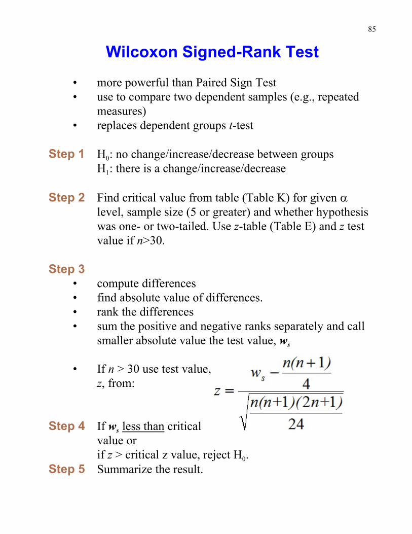
Wilcoxon Signed-Rank Test
• more powerful than Paired Sign Test• use to compare two dependent samples (e.g., repeated
measures)• replaces dependent groups t-test
Step 1 0H : no change/increase/decrease between groups
1H : there is a change/increase/decrease
Step 2 Find critical value from table (Table K) for given alevel, sample size (5 or greater) and whether hypothesiswas one- or two-tailed. Use z-table (Table E) and z testvalue if n>30.
Step 3• compute differences• find absolute value of differences.• rank the differences• sum the positive and negative ranks separately and call
ssmaller absolute value the test value, w
• If n > 30 use test value,z, from:
Step 4 sIf w less than criticalvalue or
0if z > critical z value, reject H .Step 5 Summarize the result.
86
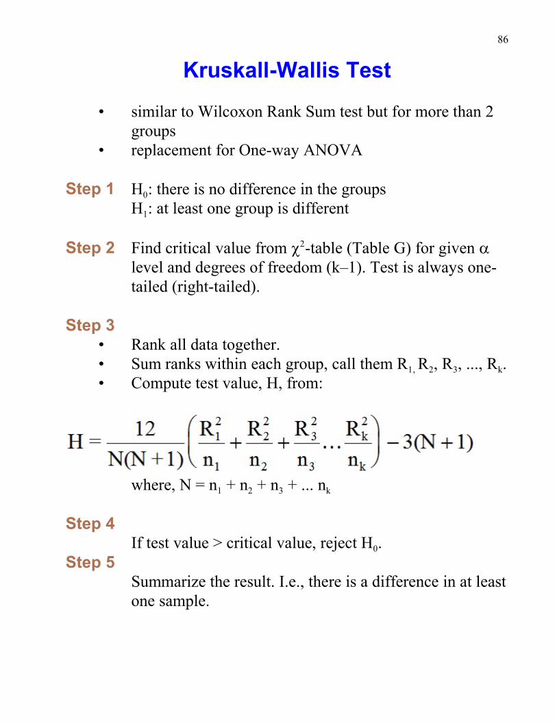
Kruskall-Wallis Test
• similar to Wilcoxon Rank Sum test but for more than 2groups
• replacement for One-way ANOVA
Step 1 0H : there is no difference in the groups
1H : at least one group is different
Step 2 Find critical value from c -table (Table G) for given a2
level and degrees of freedom (k–1). Test is always one-tailed (right-tailed).
Step 3• Rank all data together.
1, 2 3 k• Sum ranks within each group, call them R R , R , ..., R .• Compute test value, H, from:
1 2 3 kwhere, N = n + n + n + ... n
Step 4
0If test value > critical value, reject H .Step 5
Summarize the result. I.e., there is a difference in at leastone sample.
87
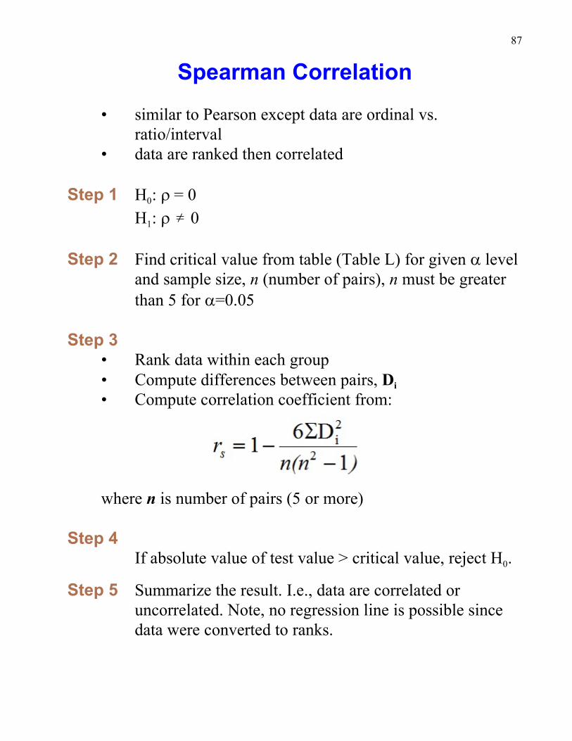
Spearman Correlation
• similar to Pearson except data are ordinal vs.ratio/interval
• data are ranked then correlated
Step 1 0H : r = 0
1H : r � 0
Step 2 Find critical value from table (Table L) for given a leveland sample size, n (number of pairs), n must be greaterthan 5 for a=0.05
Step 3• Rank data within each group
i• Compute differences between pairs, D• Compute correlation coefficient from:
where n is number of pairs (5 or more)
Step 4
0If absolute value of test value > critical value, reject H .
Step 5 Summarize the result. I.e., data are correlated oruncorrelated. Note, no regression line is possible sincedata were converted to ranks.
88
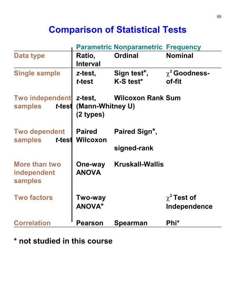
Comparison of Statistical Tests
Parametric Nonparametric FrequencyData type Ratio, Ordinal Nominal
Interval
Single sample z-test, Sign test*, c Goodness-2
t-test K-S test* of-fit
Two independent z-test, Wilcoxon Rank Sumsamples t-test (Mann-Whitney U)
(2 types)
Two dependent Paired Paired Sign*,samples t-test Wilcoxon
signed-rank
More than two One-way Kruskall-Wallisindependent ANOVAsamples
Two factors Two-way c Test of2
ANOVA* Independence
Correlation Pearson Spearman Phi*
* not studied in this course