Embed Size (px)
Citation preview

Introduction to Statistically Designed Experiments Mike Heaney ([email protected])
NREL/PR-5500-66898
ASQ Denver Section 1300 Monthly Membership Meeting September 13, 2016 Englewood, Colorado
2
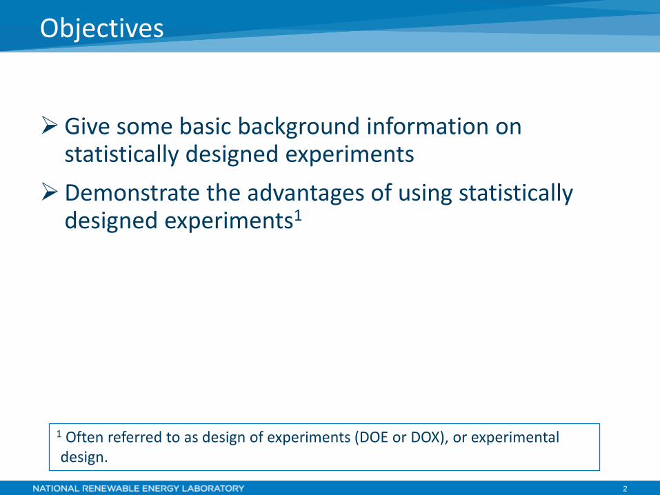
Objectives
Give some basic background information on statistically designed experiments
Demonstrate the advantages of using statistically designed experiments1
1 Often referred to as design of experiments (DOE or DOX), or experimental design.
3
A Few Thoughts
Many companies/organizations do experiments for Process improvement Product development Marketing strategies
We need to plan our experiments as efficiently and effectively as possible
Statistically designed experiments have a proven track record (Mullin 2013 in Chemical & Engineering News) Conclusions supported by statistical tests Substantial reduction in total experiments
Why are we still planning experiments like it’s the 19th century?
4
Outline
• Research Problems • The Linear Model • Key Types of Designs
o Full Factorial o Fractional Factorial o Response Surface
• Sequential Approach • Summary

Research Problems
6
Research Problems
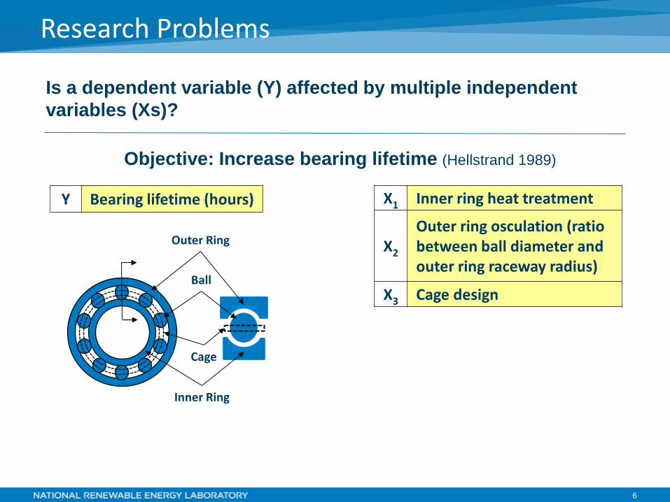
Is a dependent variable (Y) affected by multiple independent variables (Xs)?
Y Bearing lifetime (hours) X1 Inner ring heat treatment
X2
Outer ring osculation (ratio between ball diameter and outer ring raceway radius)
X3 Cage design
Objective: Increase bearing lifetime (Hellstrand 1989)
Outer Ring
Ball
Inner Ring
Cage
7
Research Problems
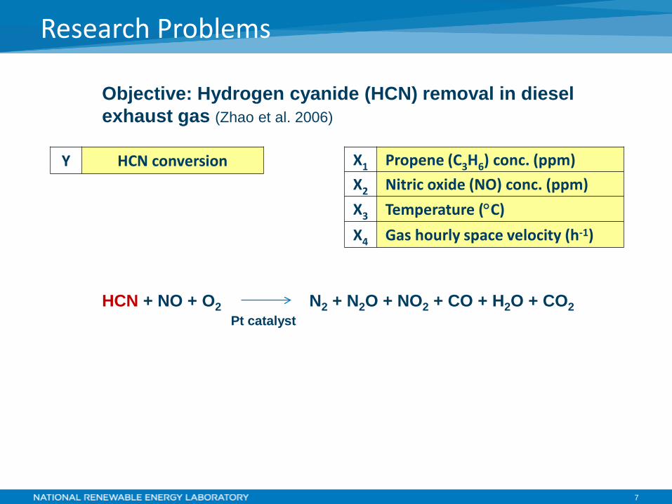
Y HCN conversion X1 Propene (C3H6) conc. (ppm) X2 Nitric oxide (NO) conc. (ppm) X3 Temperature (°C) X4 Gas hourly space velocity (h-1)
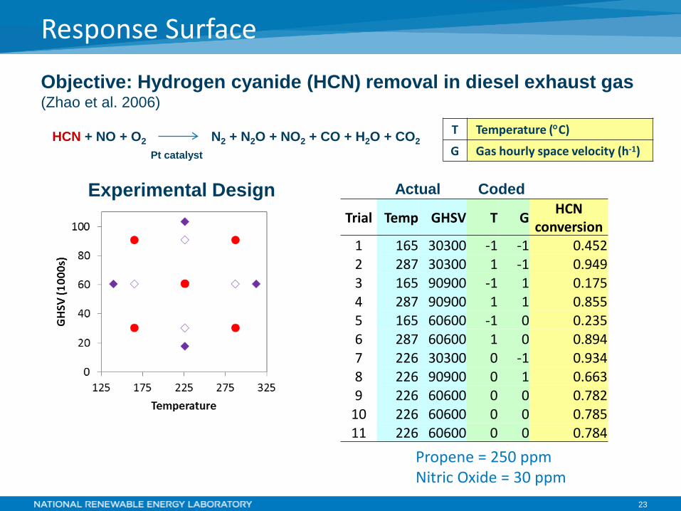
Objective: Hydrogen cyanide (HCN) removal in diesel exhaust gas (Zhao et al. 2006)
HCN + NO + O2 N2 + N2O + NO2 + CO + H2O + CO2 Pt catalyst
8
Research Problems
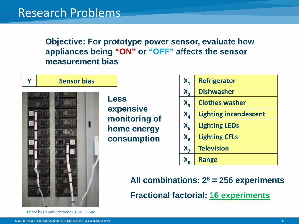
Y Sensor bias X1 Refrigerator X2 Dishwasher X3 Clothes washer X4 Lighting incandescent X5 Lighting LEDs X6 Lighting CFLs X7 Television X8 Range
Objective: For prototype power sensor, evaluate how appliances being “ON” or “OFF” affects the sensor measurement bias
All combinations: 28 = 256 experiments
Less expensive monitoring of home energy consumption
Fractional factorial: 16 experiments
Photo by Dennis Schroeder, NREL 35602

The Linear Model
10
The Linear Model
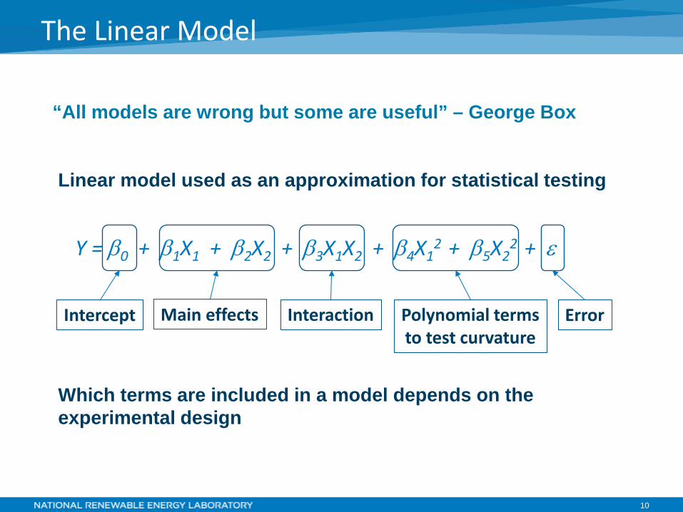
Y = β0 + β1X1 + β2X2 + β3X1X2 + β4X12
+ β5X22
+ ε
Interaction Polynomial terms to test curvature
Main effects
“All models are wrong but some are useful” – George Box
Error Intercept
Linear model used as an approximation for statistical testing
Which terms are included in a model depends on the experimental design
11
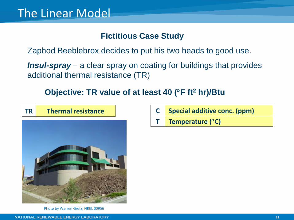
Zaphod Beeblebrox decides to put his two heads to good use.
Insul-spray − a clear spray on coating for buildings that provides additional thermal resistance (TR)
Fictitious Case Study
The Linear Model
TR Thermal resistance C Special additive conc. (ppm) T Temperature (°C)
Objective: TR value of at least 40 (°F ft2 hr)/Btu
Photo by Warren Gretz, NREL 00956
12
The Linear Model
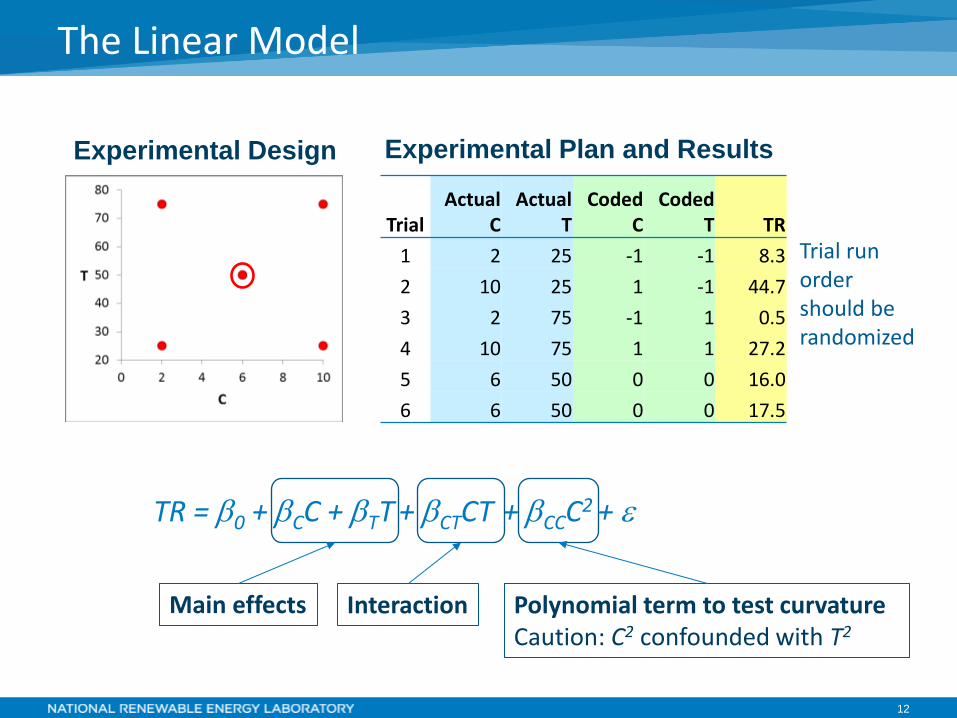
Trial run order should be randomized
Experimental Design
TR = β0 + βCC + βTT + βCTCT + βCCC2 + ε
Interaction Polynomial term to test curvature Caution: C2 confounded with T2
Trial Actual
C Actual
T Coded
C Coded
T TR 1 2 25 -1 -1 8.3 2 10 25 1 -1 44.7 3 2 75 -1 1 0.5 4 10 75 1 1 27.2 5 6 50 0 0 16.0 6 6 50 0 0 17.5
Main effects
Experimental Plan and Results
13
The Linear Model
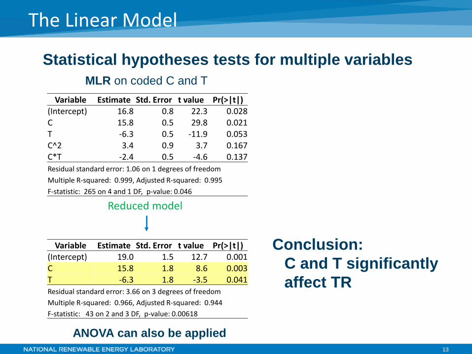
Statistical hypotheses tests for multiple variables MLR on coded C and T
Reduced model
Variable Estimate Std. Error t value Pr(>|t|) (Intercept) 16.8 0.8 22.3 0.028 C 15.8 0.5 29.8 0.021 T -6.3 0.5 -11.9 0.053 C^2 3.4 0.9 3.7 0.167 C*T -2.4 0.5 -4.6 0.137 Residual standard error: 1.06 on 1 degrees of freedom Multiple R-squared: 0.999, Adjusted R-squared: 0.995 F-statistic: 265 on 4 and 1 DF, p-value: 0.046
Variable Estimate Std. Error t value Pr(>|t|) (Intercept) 19.0 1.5 12.7 0.001 C 15.8 1.8 8.6 0.003 T -6.3 1.8 -3.5 0.041 Residual standard error: 3.66 on 3 degrees of freedom Multiple R-squared: 0.966, Adjusted R-squared: 0.944 F-statistic: 43 on 2 and 3 DF, p-value: 0.00618
ANOVA can also be applied
Conclusion: C and T significantly affect TR
14
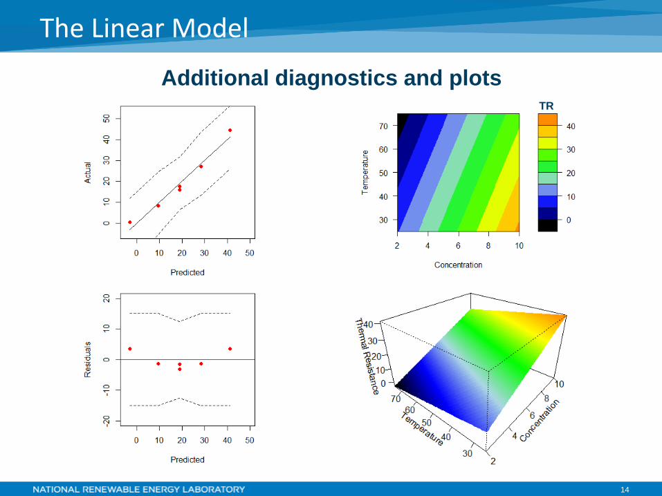
The Linear Model
Additional diagnostics and plots TR

Types of Designs
16
Full Factorial
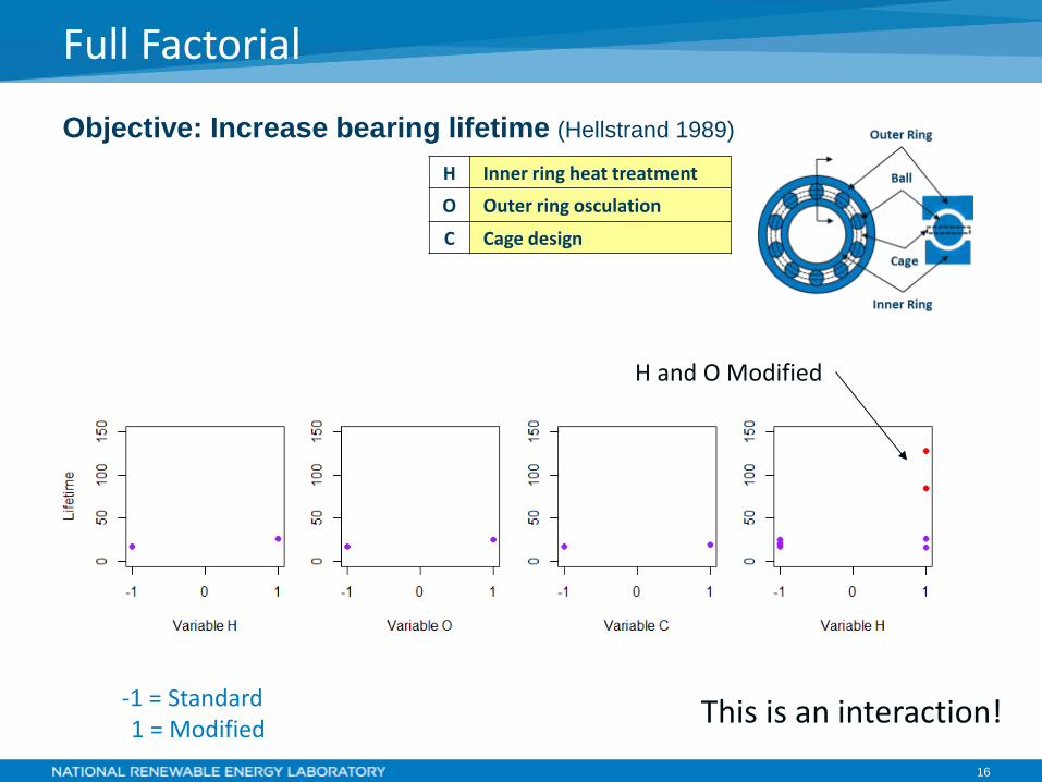
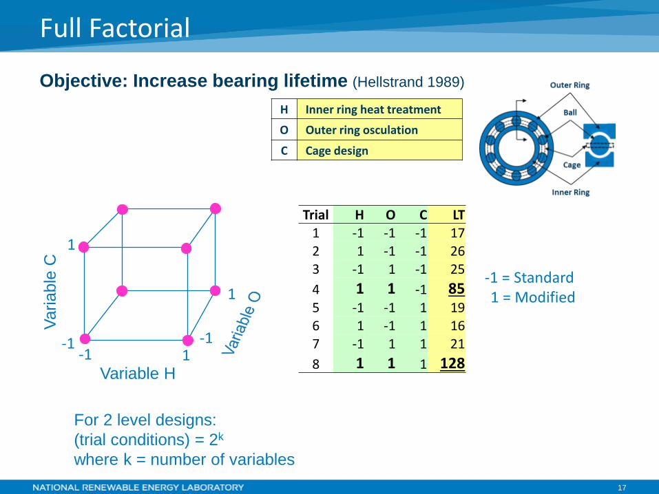
-1 = Standard 1 = Modified
Objective: Increase bearing lifetime (Hellstrand 1989)
H Inner ring heat treatment
O Outer ring osculation
C Cage design
H and O Modified
This is an interaction!
17
Full Factorial Va
riabl
e C
Variable H
-1 = Standard 1 = Modified
-1
1
-1 1 -1
1
Objective: Increase bearing lifetime (Hellstrand 1989)
For 2 level designs: (trial conditions) = 2k
where k = number of variables
Trial H O C LT 1 -1 -1 -1 17 2 1 -1 -1 26 3 -1 1 -1 25 4 1 1 -1 85 5 -1 -1 1 19 6 1 -1 1 16 7 -1 1 1 21 8 1 1 1 128
H Inner ring heat treatment
O Outer ring osculation
C Cage design
18
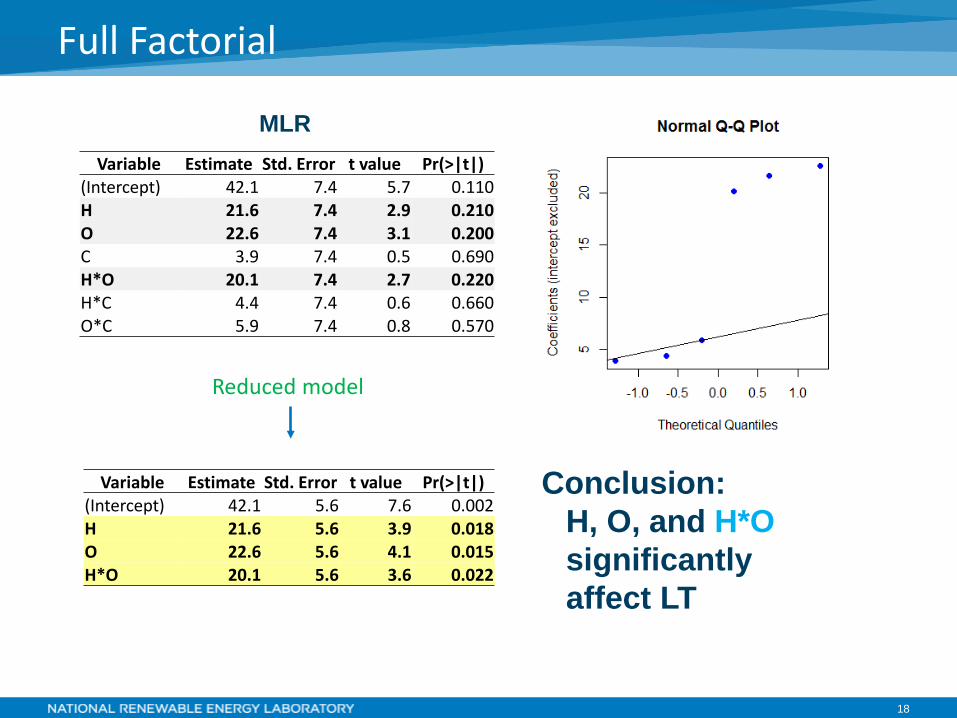
Full Factorial
Variable Estimate Std. Error t value Pr(>|t|) (Intercept) 42.1 7.4 5.7 0.110 H 21.6 7.4 2.9 0.210 O 22.6 7.4 3.1 0.200 C 3.9 7.4 0.5 0.690 H*O 20.1 7.4 2.7 0.220 H*C 4.4 7.4 0.6 0.660 O*C 5.9 7.4 0.8 0.570
MLR
Reduced model
Conclusion: H, O, and H*O significantly affect LT
Variable Estimate Std. Error t value Pr(>|t|) (Intercept) 42.1 5.6 7.6 0.002 H 21.6 5.6 3.9 0.018 O 22.6 5.6 4.1 0.015 H*O 20.1 5.6 3.6 0.022
19
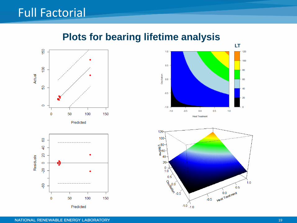
Full Factorial
Plots for bearing lifetime analysis LT

20
Fractional Factorial
Varia
ble
C
Variable A
Varia
ble
C
Variable A
Full Factorial 8 trial conditions
Fractional Factorial 4 trial conditions
Center point condition often added to test for curvature
21
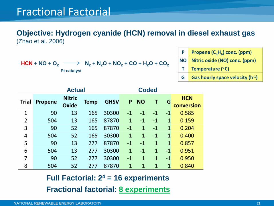
Fractional Factorial
P Propene (C3H6) conc. (ppm) NO Nitric oxide (NO) conc. (ppm) T Temperature (°C)
G Gas hourly space velocity (h-1)
Objective: Hydrogen cyanide (HCN) removal in diesel exhaust gas (Zhao et al. 2006)
HCN + NO + O2 N2 + N2O + NO2 + CO + H2O + CO2
Pt catalyst
Trial Propene Nitric Oxide Temp GHSV P NO T G HCN
conversion 1 90 13 165 30300 -1 -1 -1 -1 0.585 2 504 13 165 87870 1 -1 -1 1 0.159 3 90 52 165 87870 -1 1 -1 1 0.204 4 504 52 165 30300 1 1 -1 -1 0.400 5 90 13 277 87870 -1 -1 1 1 0.857 6 504 13 277 30300 1 -1 1 -1 0.951 7 90 52 277 30300 -1 1 1 -1 0.950 8 504 52 277 87870 1 1 1 1 0.840
Actual Coded
Full Factorial: 24 = 16 experiments Fractional factorial: 8 experiments
22
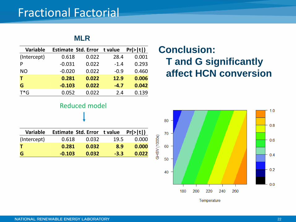
Fractional Factorial
Variable Estimate Std. Error t value Pr(>|t|) (Intercept) 0.618 0.022 28.4 0.001 P -0.031 0.022 -1.4 0.293 NO -0.020 0.022 -0.9 0.460 T 0.281 0.022 12.9 0.006 G -0.103 0.022 -4.7 0.042 T*G 0.052 0.022 2.4 0.139
MLR Conclusion:
T and G significantly affect HCN conversion
Reduced model
Variable Estimate Std. Error t value Pr(>|t|) (Intercept) 0.618 0.032 19.5 0.000 T 0.281 0.032 8.9 0.000 G -0.103 0.032 -3.3 0.022
23
Response Surface
T Temperature (°C)
G Gas hourly space velocity (h-1)
Objective: Hydrogen cyanide (HCN) removal in diesel exhaust gas (Zhao et al. 2006)
HCN + NO + O2 N2 + N2O + NO2 + CO + H2O + CO2
Pt catalyst
Actual Coded
Trial Temp GHSV T G HCN conversion
1 165 30300 -1 -1 0.452 2 287 30300 1 -1 0.949 3 165 90900 -1 1 0.175 4 287 90900 1 1 0.855 5 165 60600 -1 0 0.235 6 287 60600 1 0 0.894 7 226 30300 0 -1 0.934 8 226 90900 0 1 0.663 9 226 60600 0 0 0.782
10 226 60600 0 0 0.785 11 226 60600 0 0 0.784
Propene = 250 ppm Nitric Oxide = 30 ppm
Experimental Design
24
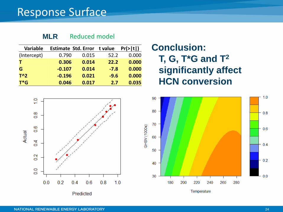
Response Surface
Variable Estimate Std. Error t value Pr(>|t|) (Intercept) 0.790 0.015 52.2 0.000 T 0.306 0.014 22.2 0.000 G -0.107 0.014 -7.8 0.000 T^2 -0.196 0.021 -9.6 0.000 T*G 0.046 0.017 2.7 0.035
MLR Reduced model
Conclusion: T, G, T*G and T2 significantly affect HCN conversion

Sequential Approach
26
Sequential Approach
Basic idea is to break up overall experimental plan into a few complementary experimental plans
Start simple (fractional factorials) - 25% rule (25-40% of allotted time/effort in first designed experiment)
Modify additional experiments based on what is learned from prior experiments
BE FLEXIBLE!!!
General concepts of sequential approach (Box and Bisgaard 1997)
27
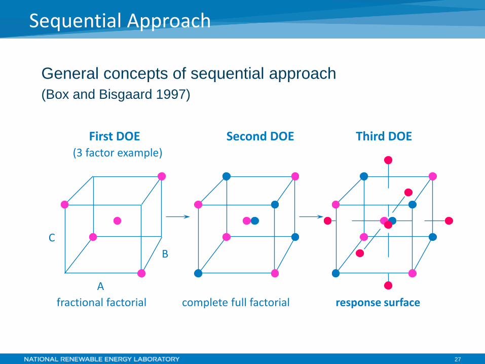
Sequential Approach
General concepts of sequential approach (Box and Bisgaard 1997)
A
B C
(3 factor example) First DOE Second DOE
complete full factorial fractional factorial response surface
Third DOE
28
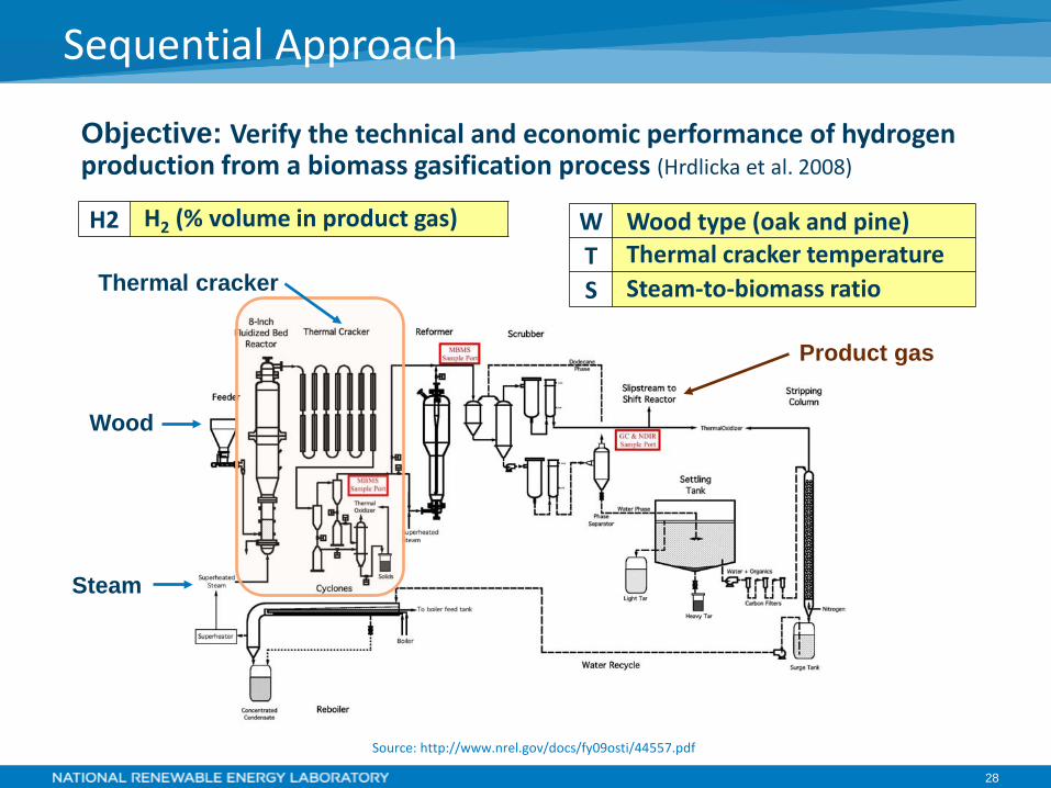
Sequential Approach
H2 H2 (% volume in product gas) W Wood type (oak and pine) T Thermal cracker temperature S Steam-to-biomass ratio
Objective: Verify the technical and economic performance of hydrogen production from a biomass gasification process (Hrdlicka et al. 2008)
Source: http://www.nrel.gov/docs/fy09osti/44557.pdf
Wood
Steam
Thermal cracker
Product gas
29
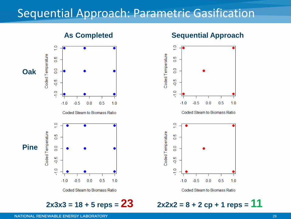
Sequential Approach: Parametric Gasification
As Completed
Oak
Pine
2x3x3 = 18 + 5 reps = 23
Sequential Approach
2x2x2 = 8 + 2 cp + 1 reps = 11
30
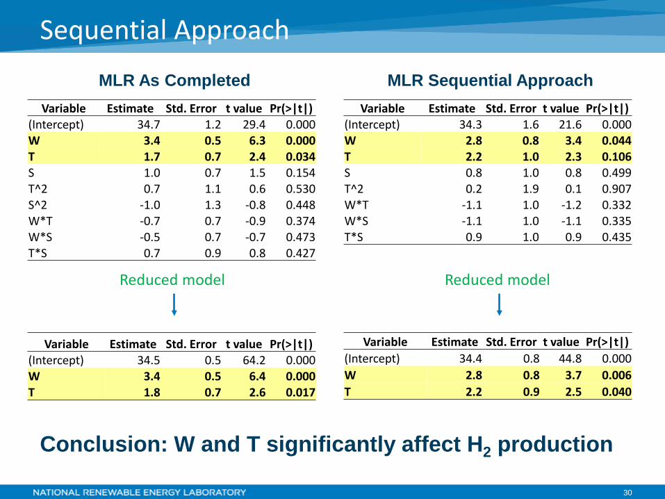
Sequential Approach
Reduced model
MLR As Completed MLR Sequential Approach Variable Estimate Std. Error t value Pr(>|t|)
(Intercept) 34.7 1.2 29.4 0.000 W 3.4 0.5 6.3 0.000 T 1.7 0.7 2.4 0.034 S 1.0 0.7 1.5 0.154 T^2 0.7 1.1 0.6 0.530 S^2 -1.0 1.3 -0.8 0.448 W*T -0.7 0.7 -0.9 0.374 W*S -0.5 0.7 -0.7 0.473 T*S 0.7 0.9 0.8 0.427
Variable Estimate Std. Error t value Pr(>|t|) (Intercept) 34.5 0.5 64.2 0.000 W 3.4 0.5 6.4 0.000 T 1.8 0.7 2.6 0.017
Variable Estimate Std. Error t value Pr(>|t|) (Intercept) 34.3 1.6 21.6 0.000 W 2.8 0.8 3.4 0.044 T 2.2 1.0 2.3 0.106 S 0.8 1.0 0.8 0.499 T^2 0.2 1.9 0.1 0.907 W*T -1.1 1.0 -1.2 0.332 W*S -1.1 1.0 -1.1 0.335 T*S 0.9 1.0 0.9 0.435
Variable Estimate Std. Error t value Pr(>|t|) (Intercept) 34.4 0.8 44.8 0.000 W 2.8 0.8 3.7 0.006 T 2.2 0.9 2.5 0.040
Reduced model
Conclusion: W and T significantly affect H2 production
31
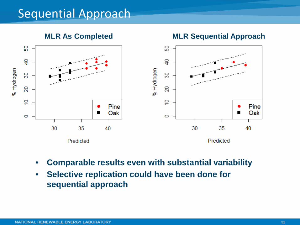
Sequential Approach
MLR As Completed MLR Sequential Approach
• Comparable results even with substantial variability • Selective replication could have been done for
sequential approach
32
Summary
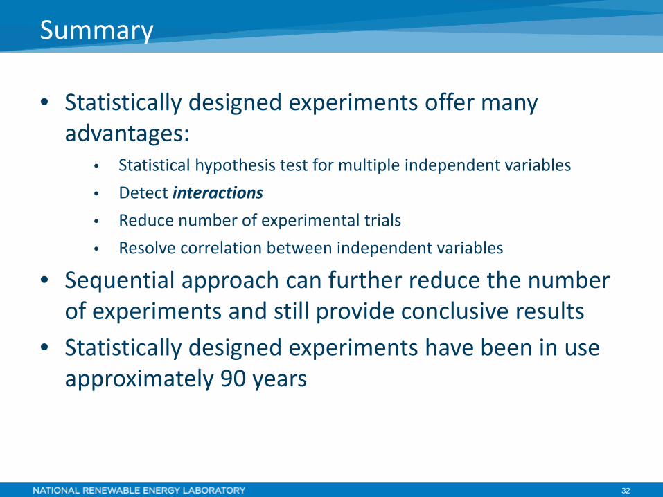
• Statistically designed experiments offer many advantages:
• Statistical hypothesis test for multiple independent variables • Detect interactions • Reduce number of experimental trials • Resolve correlation between independent variables
• Sequential approach can further reduce the number of experiments and still provide conclusive results
• Statistically designed experiments have been in use approximately 90 years

Supplemental Slides
35
References
Box, G.E.P. and Bisgaard, S. (1997). Design of Experiments for Discovery, Improvement and Robustness: Going Beyond the Basic Principles. The College of Engineering, University of Wisconsin, Madison, WI.
Hellstrand, C. (1989). The Necessity of Modern Quality Improvement and Some Experience With its Implementation in the Manufacture of Rolling Bearings. The College of Engineering, University of Wisconsin, Madison, WI. Accessed January 11, 2012: http://cqpi.engr.wisc.edu/system/files/r035.pdf.
Hrdlicka, J.; Feik, C.; Carpenter, D.; Pomeroy, M. (2008). Parametric Gasification of Oak and Pine Feedstocks Using the TCPDU and Slipstream Water-Gas Shift Catalysis. Golden, CO: National Renewable Energy Laboratory, NREL/TP-510-44557.
Mullin, R. (2013). “Design Of Experiments Makes A Comeback.” Chemical & Engineering News, Volume 91 Issue 13, pp 25-28. Accessed November 19, 2015: http://cen.acs.org/articles/91/i13/Design-Experiments-Makes-Comeback.html?h=2027056365.
Zhao, H; Tonkyn, R.; Barlow, S.; Peden, C; Koel, B. (2006). “Fractional Factorial Study of HCN Removal over 0.5% Pt/Al2O3 Catalyst: Effects of Temperature, Gas Flow Rate, and Reactant Partial Pressure.” Industrial & Engineering Chemistry Research, Volume 45, pp 934-939.

36
Bibliography
Box, G.E.P., Hunter, W.G. and Hunter, J.S. (1978). Statistics for Experimenters. John Wiley & Sons.
Deming, W.E. (1986). Out of the Crisis. Massachusetts Institute of Technology, Cambridge, MA.
Gunst, R.F. and Mason, R.L. (1991). Volume 14: How to Construct Fractional Factorial Experiments. ASQ Quality Press, Milwaukee, WI.
Montgomery, D.C. (1997). Design and Analysis of Experiments, Fourth Edition. John Wiley & Sons.
NIST (2015). Engineering Statistics Handbook. Accessed December 1, 2015: http://www.itl.nist.gov/div898/handbook/index.htm.
R Core Team (2014). “R: A Language and Environment for Statistical Computing.” Vienna, Austria: R Foundation for Statistical Computing. Accessed April 6, 2015: http://www.R-project.org/.
Rodríguez, G. (2013). “Introducing R.” Princeton University, Accessed January 13, 2014: http://data.princeton.edu/R/linearModels.html.
37
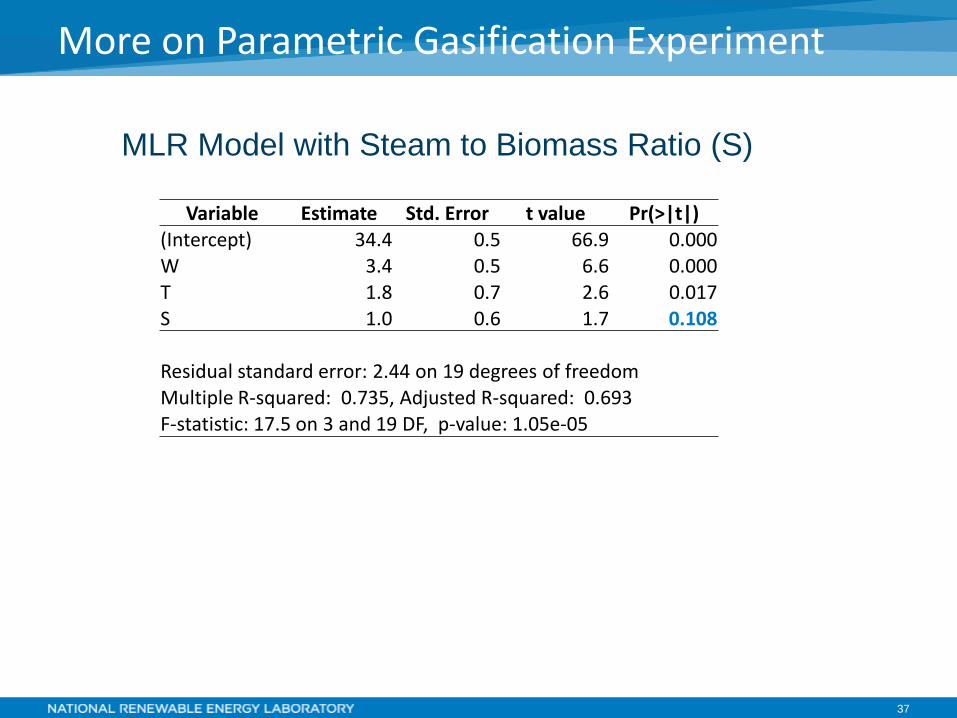
More on Parametric Gasification Experiment
MLR Model with Steam to Biomass Ratio (S)
Variable Estimate Std. Error t value Pr(>|t|) (Intercept) 34.4 0.5 66.9 0.000 W 3.4 0.5 6.6 0.000 T 1.8 0.7 2.6 0.017 S 1.0 0.6 1.7 0.108
Residual standard error: 2.44 on 19 degrees of freedom Multiple R-squared: 0.735, Adjusted R-squared: 0.693 F-statistic: 17.5 on 3 and 19 DF, p-value: 1.05e-05