INTRODUCTION TO STATIC ANALYSIS

PDPI 2013

What is “Pile Capacity” ?

When we load a pile until IT Fails – what is “IT”

Strength Considerations Two Failure Modes

1. Pile structural failure

controlled by allowable driving stresses

2. Soil failure

controlled by factor of safety (ASD) resistance factors (LRFD)

In addition, driveability is evaluated by wave equation

STATIC ANALYSIS METHODS

Designer should fully know the basis for, limitations

of, and applicability of a chosen method.

Foundation designer must know design loads and

performance requirements.

Many static analysis methods are available.

- methods in manual are relatively simple

- methods provide reasonable agreement with full scale tests

- other more sophisticated methods could be used

BASICS OF STATIC ANALYSIS

Static capacity is the sum of the soil/rock

resistances along the pile shaft and at the pile toe.

Static analyses are performed to determine ultimate

pile capacity and the pile group response to applied

loads.

The ultimate capacity of a pile and pile group is the

smaller of the soil rock medium to support the pile

loads or the structural capacity of the piles.

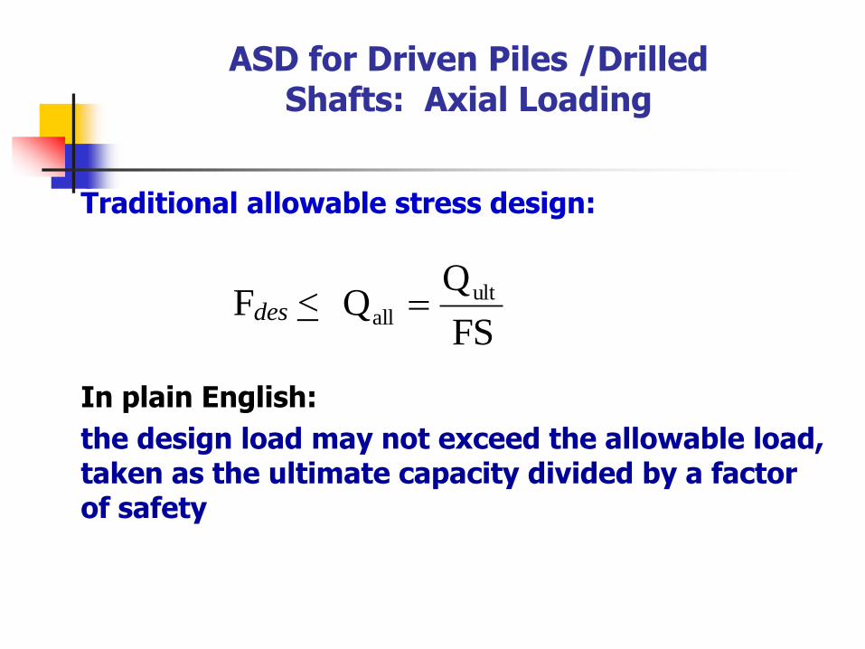
ASD for Driven Piles /Drilled Shafts: Axial Loading

Traditional allowable stress design:

In plain English:

the design load may not exceed the allowable load, taken as the ultimate capacity divided by a factor of safety

Fdes < FS

QQ ult

all

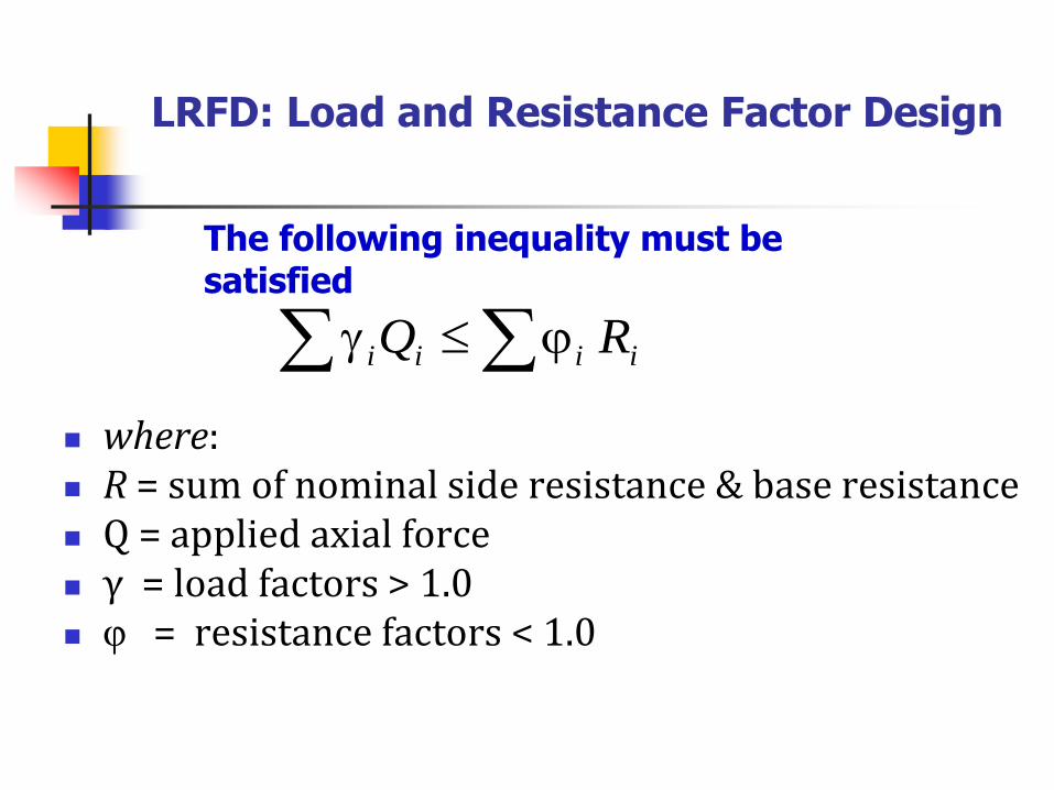
LRFD: Load and Resistance Factor Design

where: R = sum of nominal side resistance & base resistance Q = applied axial force γ = load factors > 1.0 φ = resistance factors < 1.0

In plain English:

the summation of factored force effects must not

exceed the summation of factored resistances

iiii RQ

The following inequality must be satisfied

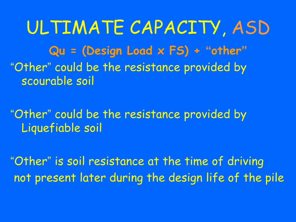
ULTIMATE CAPACITY, ASD Qu = (Design Load x FS) + “other”

“Other” could be the resistance provided by scourable soil

“Other” could be the resistance provided by Liquefiable soil

“Other” is soil resistance at the time of driving

not present later during the design life of the pile

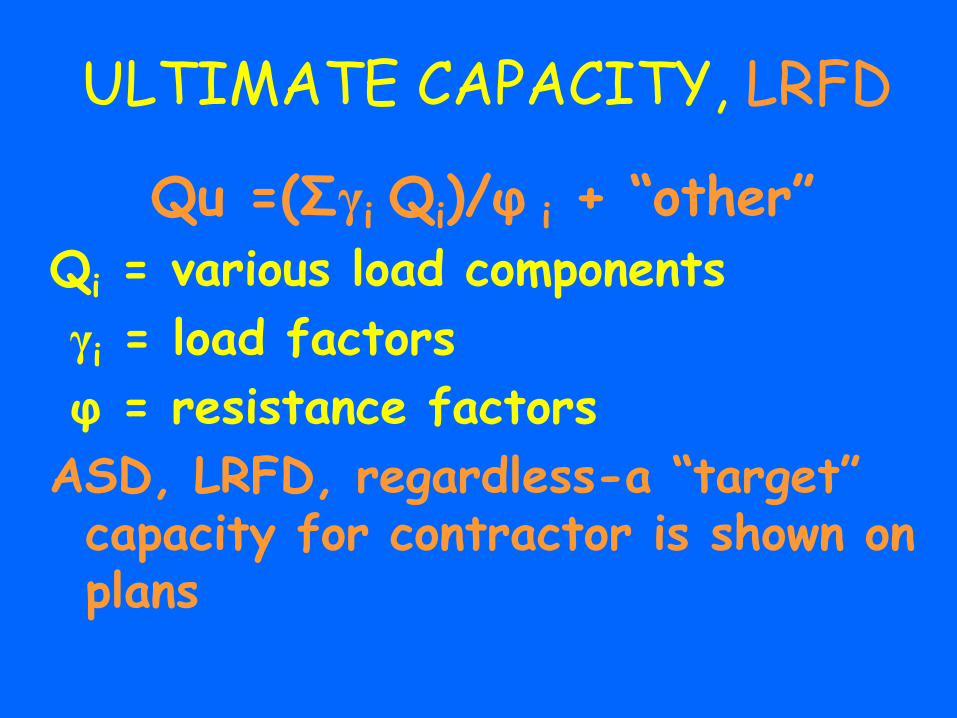
ULTIMATE CAPACITY, LRFD

Qu =(Σγi Qi)/φ i + “other” Qi = various load components

γi = load factors

φ = resistance factors

ASD, LRFD, regardless-a “target” capacity for contractor is shown on plans

LRFD

Structural Engineer

Estimates, magnitude and direction of loads:

Geotechnical Engineer

Estimates soil resistance and calculates size, length and quantity of piles to resist the given loads.

The factored resistance must be greater than the factored applied loads !

Any SCOUR ?? Any SET UP

Pro

fesso

r's D

rive

n P

ile In

stitu

te, U

tah

Sta

te U

niv

ers

ity

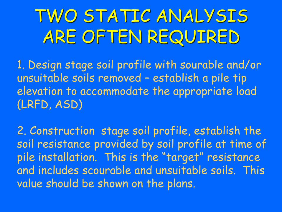
TWO STATIC ANALYSIS ARE OFTEN REQUIRED

1. Design stage soil profile with sourable and/or unsuitable soils removed – establish a pile tip elevation to accommodate the appropriate load (LRFD, ASD) 2. Construction stage soil profile, establish the soil resistance provided by soil profile at time of pile installation. This is the “target” resistance and includes scourable and unsuitable soils. This value should be shown on the plans.

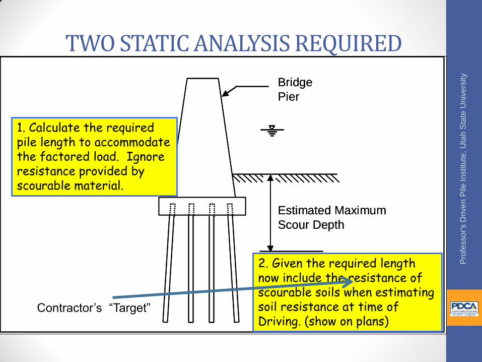
TWO STATIC ANALYSIS REQUIRED

Estimated Maximum

Scour Depth

Bridge

Pier

Estimated Maximum

Scour Depth

Bridge

Pier

2. Given the required length now include the resistance of scourable soils when estimating soil resistance at time of Driving. (show on plans)

Pro

fesso

r's D

rive

n P

ile In

stitu

te, U

tah

Sta

te U

niv

ers

ity

1. Calculate the required pile length to accommodate the factored load. Ignore resistance provided by scourable material.

Contractor’s “Target”

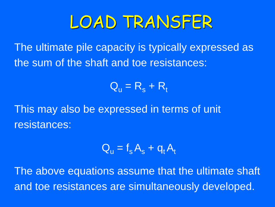
LOAD TRANSFER

The ultimate pile capacity is typically expressed as

the sum of the shaft and toe resistances:

Qu = Rs + Rt

This may also be expressed in terms of unit

resistances:

Qu = fs As + qt At

The above equations assume that the ultimate shaft

and toe resistances are simultaneously developed.

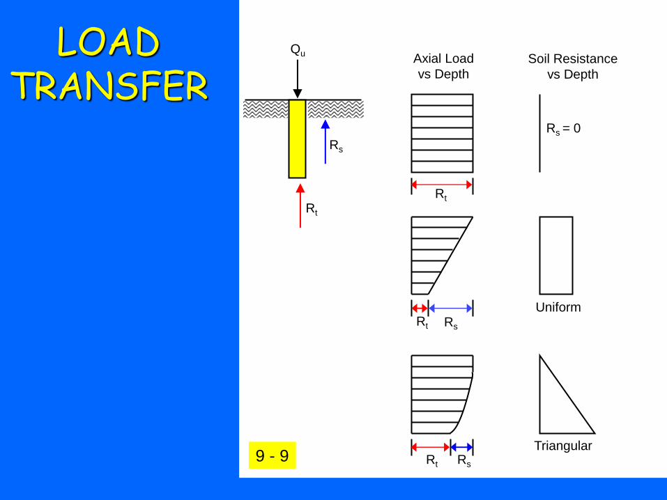
LOAD TRANSFER

Rt

Axial Load

vs Depth

Rt

Rs

Qu

Rs

Soil Resistance

vs Depth

Rs = 0

Uniform

Triangular

Rs Rt

Rt

9 - 9

DESIGN SOIL STRENGTH PARAMETERS

Most of the static analysis methods in cohesionless

soils use the soil friction angle determined from

laboratory tests or SPT N values.

In coarse granular deposits, the soil friction angle

should be chosen conservatively.

What does this mean ??

DESIGN SOIL STRENGTH PARAMETERS

In soft, rounded gravel deposits, use a maximum

soil friction angle, , of 32˚ for shaft resistance

calculations.

In hard, angular gravel deposits, use a maximum

friction angle of 36˚ for shaft resistance

calculations.

DESIGN SOIL STRENGTH PARAMETERS

In cohesive soils, accurate assessments of the soil

shear strength and consolidation properties are

needed for static analysis.

The sensitivity of cohesive soils should be known

during the design stage so that informed

assessments of pile driveability and soil setup can

be made.

DESIGN SOIL STRENGTH PARAMETERS

For a cost effective design with any static analysis

method, the foundation designer must consider

time dependent soil strength changes.

Ignore set up --- uneconomical

Ignore relaxation --- unsafe

Static Analysis - Single Piles

Methods for estimating axial static

resistance of soils

Soil Mechanics Review

• Angle of friction

• Undrained shear strength

• Unconfined Compression Strength

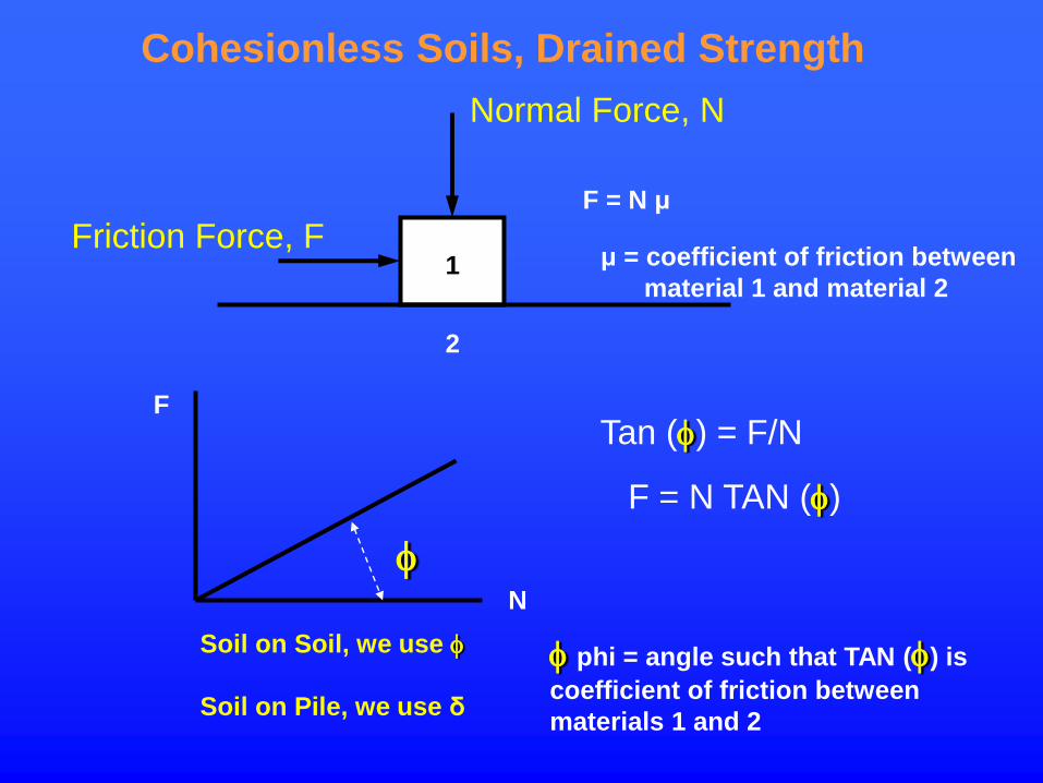
Normal Force, N

Friction Force, F F = N μ

μ = coefficient of friction between

material 1 and material 2

F

N

Tan () = F/N

F = N TAN ()

phi = angle such that TAN () is

coefficient of friction between

materials 1 and 2

1

2

Soil on Soil, we use

Soil on Pile, we use δ

Cohesionless Soils, Drained Strength

Cohesive Soils, Undrained Strength

F

N

c

= zero

c = cohesion, stickiness, soil / soil

a = adhesion, stickiness, soil / pile

C is independent of overburden pressures (i.e. N)

F = Friction resistance (stress) N = Normal force (stress)

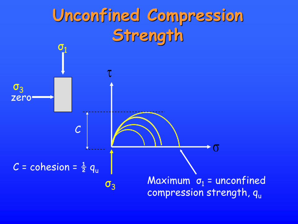
Unconfined Compression Strength

zero

Maximum σ1 = unconfined compression strength, qu

C

C = cohesion = ½ qu

σ1

σ3

σ3

STATIC CAPACITY

OF PILES IN

COHESIONLESS SOILS

METHODS OF STATIC ANALYSIS FOR PILES IN COHESIONLESS SOILS

Method Approach Design

Parameters

Advantages Disadvantages Remarks

Meyerhof

Method

Empirical Results of

SPT tests.

Widespread use of

SPT test and input

data availability.

Simple method to

use.

Non

reproducibility of

N values. Not

as reliable as the

other methods

presented in this

chapter.

Due to non

reproducibility of N

values and

simplifying

assumptions, use

should be limited to

preliminary

estimating

purposes.

Brown

Method

Empirical Results of

SPT tests

based of N60

values.

Widespread use of

SPT test and input

data availability.

Simple method to

use.

N60 values not

always

available.

Simple method

based on

correlations with 71

static load test

results. Details

provided in Section

9.7.1.1b.

Nordlund

Method.

Semi-

empirical

Charts

provided by

Nordlund.

Estimate of

soil friction

angle is

needed.

Allows for

increased shaft

resistance of

tapered piles and

includes effects of

pile-soil friction

coefficient for

different pile

materials.

No limiting value

on unit shaft

resistance is

recommended

by Nordlund.

Soil friction

angle often

estimated from

SPT data.

Good approach to

design that is

widely used.

Method is based on

field observations.

Details provided in

Section 9.7.1.1c.

FHWA

9-19

Part Theory

Part

Experience

Experience N

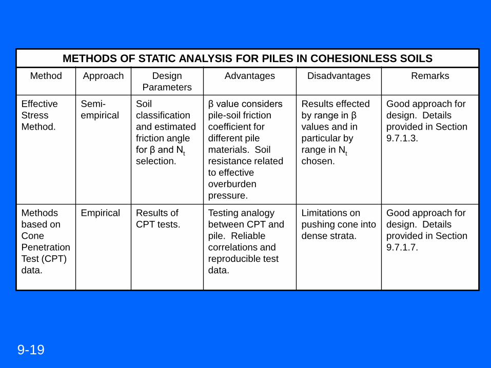
METHODS OF STATIC ANALYSIS FOR PILES IN COHESIONLESS SOILS

Method Approach Design

Parameters

Advantages Disadvantages Remarks

Effective

Stress

Method.

Semi-

empirical

Soil

classification

and estimated

friction angle

for β and Nt

selection.

β value considers

pile-soil friction

coefficient for

different pile

materials. Soil

resistance related

to effective

overburden

pressure.

Results effected

by range in β

values and in

particular by

range in Nt

chosen.

Good approach for

design. Details

provided in Section

9.7.1.3.

Methods

based on

Cone

Penetration

Test (CPT)

data.

Empirical Results of

CPT tests.

Testing analogy

between CPT and

pile. Reliable

correlations and

reproducible test

data.

Limitations on

pushing cone into

dense strata.

Good approach for

design. Details

provided in Section

9.7.1.7.

9-19

Nordlund Data Base

Pile Types

Pile Sizes

Pile Loads

Timber, H-piles, Closed-end Pipe,

Monotube, Raymond Step-Taper

Pile widths of 250 – 500 mm (10 - 20 in)

Ultimate pile capacities of 350 -2700 kN

(40 -300 tons)

Nordlund Method tends to overpredict capacity

of piles greater than 600 mm (24 in) 9-25

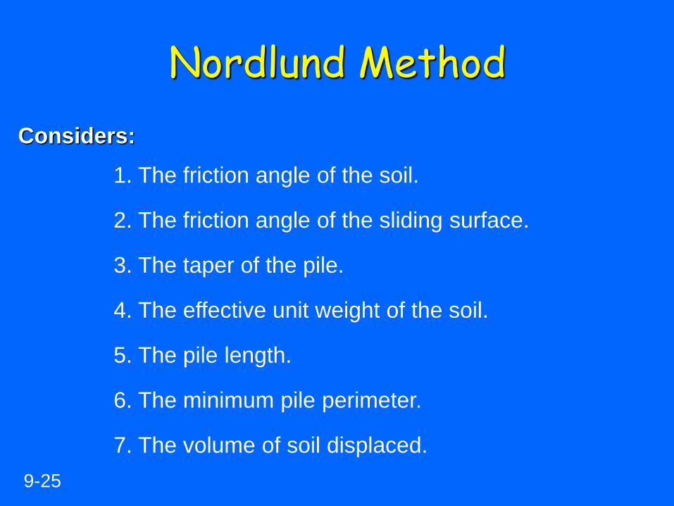
Nordlund Method

1. The friction angle of the soil.

9-25

2. The friction angle of the sliding surface.

3. The taper of the pile.

4. The effective unit weight of the soil.

5. The pile length.

6. The minimum pile perimeter.

7. The volume of soil displaced.

Considers:

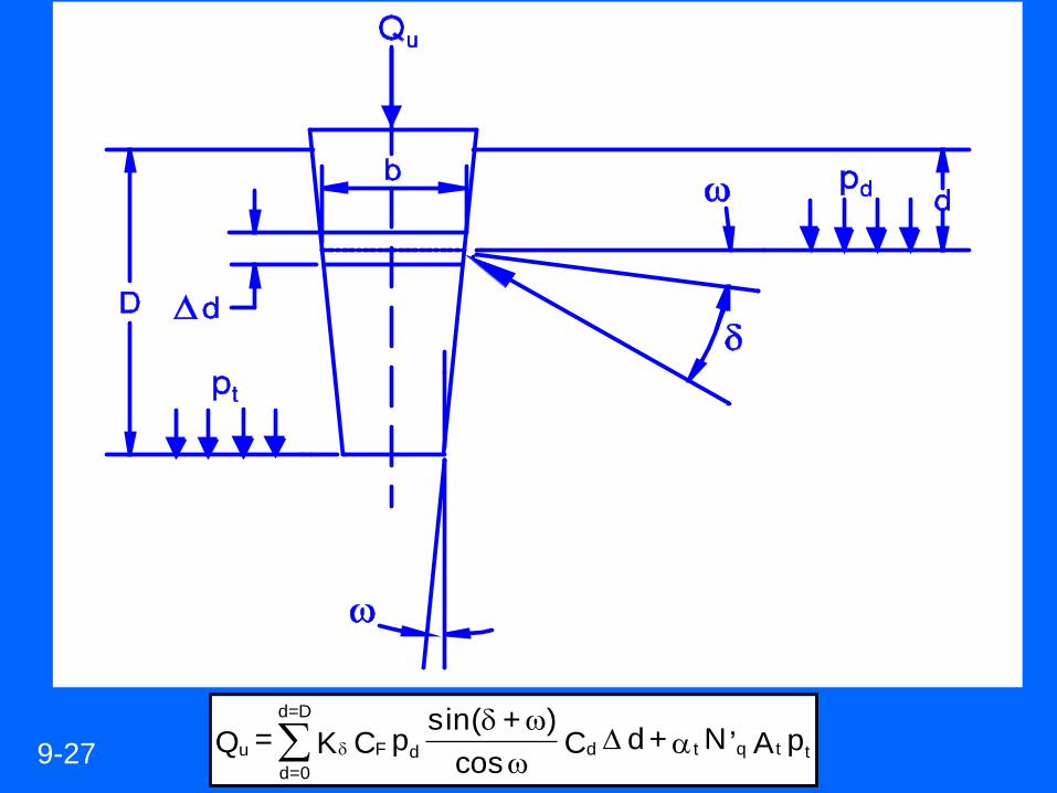
p A ’N + d C cos

) + ( sin p C K = Q ttqtddF

D=d

0=d

u

9-27

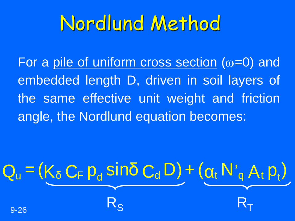
For a pile of uniform cross section (=0) and

embedded length D, driven in soil layers of

the same effective unit weight and friction

angle, the Nordlund equation becomes:

)p A ’N α( + D) C sinδ p C K( = Q ttqtddFδu

Nordlund Method

RS RT 9-26

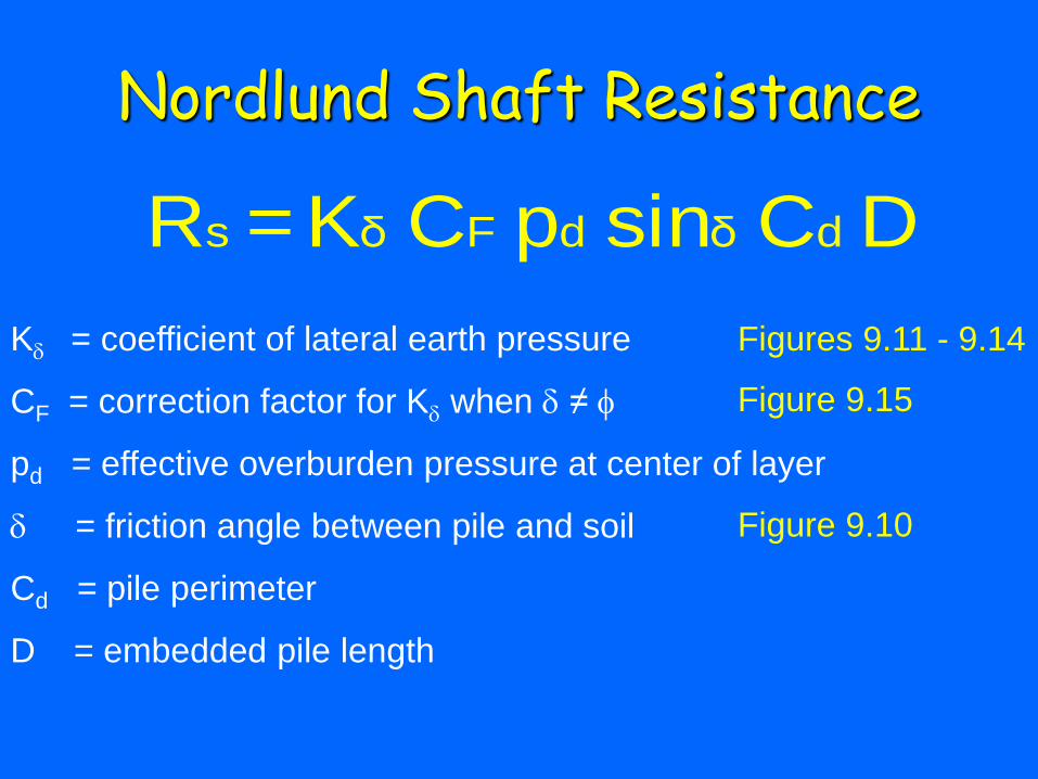
Nordlund Shaft Resistance

DCsinpCK = R d δ d F δs

K = coefficient of lateral earth pressure

CF = correction factor for K when ≠

pd = effective overburden pressure at center of layer

= friction angle between pile and soil

Cd = pile perimeter

D = embedded pile length

Figures 9.11 - 9.14

Figure 9.15

Figure 9.10

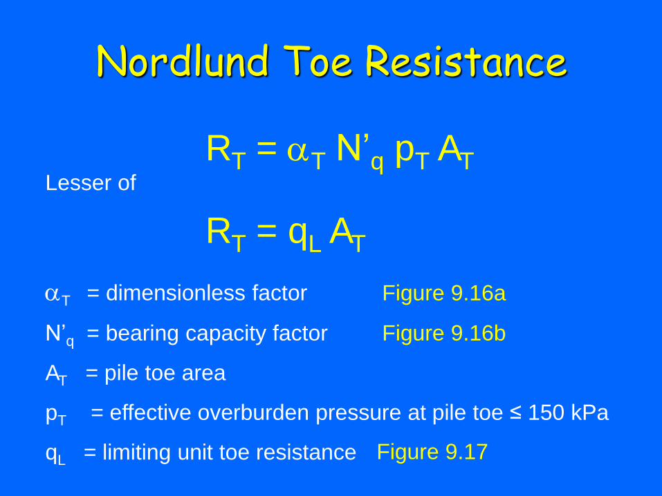
Nordlund Toe Resistance

T = dimensionless factor

N’q = bearing capacity factor

AT = pile toe area

pT = effective overburden pressure at pile toe ≤ 150 kPa

qL = limiting unit toe resistance

Figure 9.16a

Figure 9.16b

Figure 9.17

RT = qL AT

RT = T N’q pT AT Lesser of

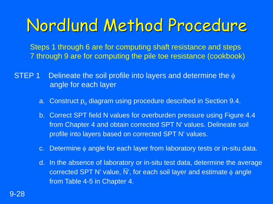
Nordlund Method Procedure Steps 1 through 6 are for computing shaft resistance and steps

7 through 9 are for computing the pile toe resistance (cookbook)

STEP 1 Delineate the soil profile into layers and determine the

angle for each layer

a. Construct po diagram using procedure described in Section 9.4.

b. Correct SPT field N values for overburden pressure using Figure 4.4

from Chapter 4 and obtain corrected SPT N' values. Delineate soil

profile into layers based on corrected SPT N' values.

c. Determine angle for each layer from laboratory tests or in-situ data.

d. In the absence of laboratory or in-situ test data, determine the average

corrected SPT N' value, N', for each soil layer and estimate angle

from Table 4-5 in Chapter 4.

9-28

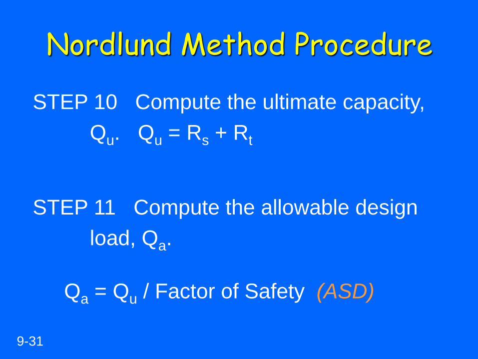
Nordlund Method Procedure

STEP 10 Compute the ultimate capacity,

Qu. Qu = Rs + Rt

9-31

STEP 11 Compute the allowable design

load, Qa.

Qa = Qu / Factor of Safety (ASD)

STATIC CAPACITY

OF PILES IN

COHESIVE SOILS

METHODS OF STATIC ANALYSIS FOR PILES IN COHESIVE SOILS

Method Approach Method of

Obtaining

Design Parameters

Advantages Disadvantages Remarks

α-Method

(Tomlinson

Method).

Empirical,

total stress

analysis.

Undrained shear

strength estimate

of soil is needed.

Adhesion

calculated from

Figures 9.18 and

9.19.

Simple calculation

from laboratory

undrained shear

strength values to

adhesion.

Wide scatter in

adhesion versus

undrained shear

strengths in

literature.

Widely used

method

described in

Section

9.7.1.2a.

Effective

Stress

Method.

Semi-

Empirical,

based on

effective

stress at

failure.

β and Nt values

are selected from

Table 9-6 based on

drained soil

strength estimates.

Ranges in β and

Nt values for

most cohesive

soils are relatively

small.

Range in Nt

values for hard

cohesive soils

such as glacial

tills can be large.

Good design

approach

theoretically

better than

undrained

analysis.

Details in

Section

9.7.1.3.

Methods

based on

Cone

Penetration

Test data.

Empirical. Results of CPT

tests.

Testing analogy

between CPT and

pile.

Reproducible test

data.

Cone can be

difficult to

advance in very

hard cohesive

soils such as

glacial tills.

Good

approach for

design.

Details in

Section

9.7.1.7.

FHWA

9-42

Tomlinson or α-Method

Unit Shaft Resistance, fs:

fs = ca = αcu

Where:

ca = adhesion (Figure 9.18)

α = empirical adhesion factor (Figure 9.19)

9-41

Tomlinson or α-Method

Shaft Resistance, Rs:

Rs = fs As

Where:

As = pile surface area in layer

(pile perimeter x

length)

Concrete, Timber, Corrugated Steel Piles

Smooth Steel Piles b = Pile Diameter

D = distance from ground surface to bottom of

clay layer or pile toe, whichever is less

Tomlinson or α-Method (US)

Figure 9.18

Tomlinson or α-Method

Unit Toe Resistance, qt:

qt = cu Nc

Where:

cu = undrained shear strength of the soil at pile toe

Nc = dimensionless bearing capacity factor

(9 for deep foundations)

Tomlinson or α-Method

Toe Resistance, Rt:

Rt = qt At

The toe resistance in cohesive soils is sometimes ignored

since the movement required to mobilize the toe resistance

is several times greater than the movement required to

mobilize the shaft resistance.

Ru = RS + RT

Qa = RU / FS

and

Tomlinson or α-Method

9-56

DRIVEN COMPUTER PROGRAM

Can be used to calculate the static capacity of

open and closed end pipe piles, H-piles, circular or

square solid concrete piles, timber piles, and

Monotube piles.

Analyses can be performed in SI or US units.

DRIVEN uses the FHWA recommended Nordlund

(cohesionless) and α-methods (cohesive).

Available at: www.fhwa.dot.gov/bridge/geosoft.htm

The Pile Design is not complete until the pile

has been driven – that’s when we can estimate

the “capacity” (E.O.D)

STATIC ANALYSIS – SINGLE PILES

LATERAL CAPACITY METHODS

Reference Manual Chapter 9.7.3

9-82

Lateral Capacity of Single Piles

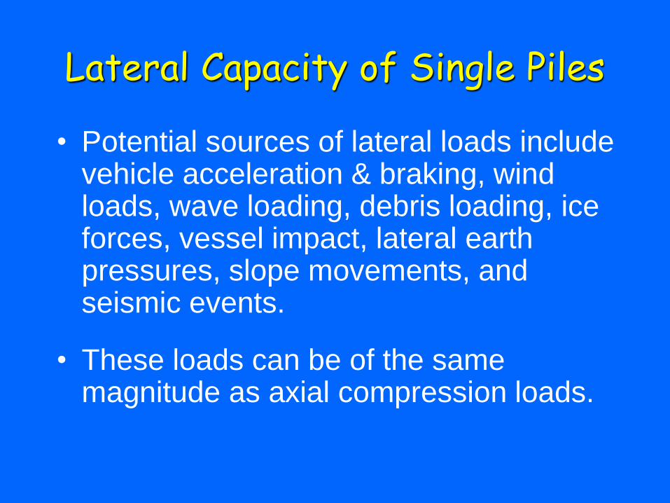
• Potential sources of lateral loads include vehicle acceleration & braking, wind loads, wave loading, debris loading, ice forces, vessel impact, lateral earth pressures, slope movements, and seismic events.

• These loads can be of the same magnitude as axial compression loads.

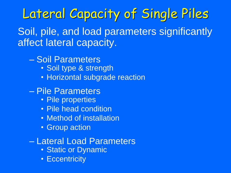
Lateral Capacity of Single Piles Soil, pile, and load parameters significantly affect lateral capacity.

– Soil Parameters • Soil type & strength

• Horizontal subgrade reaction

– Pile Parameters • Pile properties

• Pile head condition

• Method of installation

• Group action

– Lateral Load Parameters • Static or Dynamic

• Eccentricity

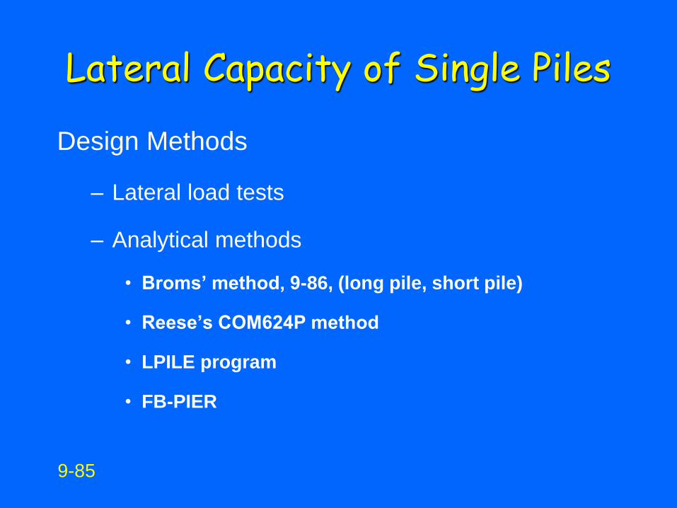
Lateral Capacity of Single Piles

Design Methods

– Lateral load tests

– Analytical methods

• Broms’ method, 9-86, (long pile, short pile)

• Reese’s COM624P method

• LPILE program

• FB-PIER

9-85

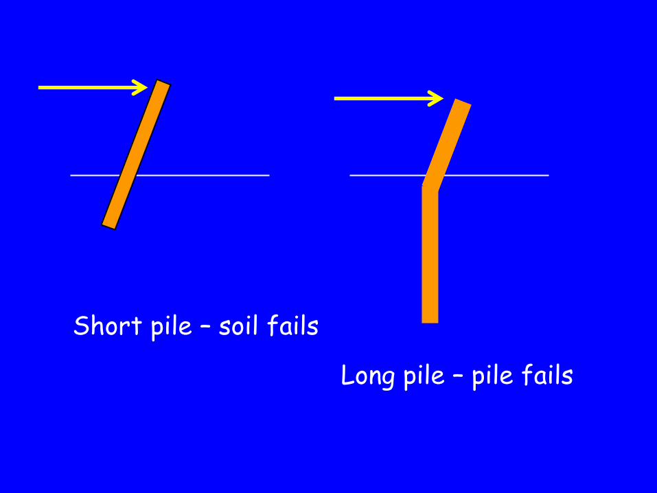
Long pile – pile fails

Short pile – soil fails

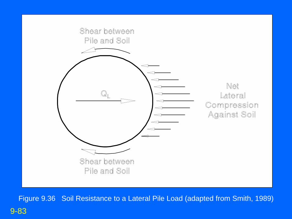
Figure 9.36 Soil Resistance to a Lateral Pile Load (adapted from Smith, 1989)

9-83

NIM

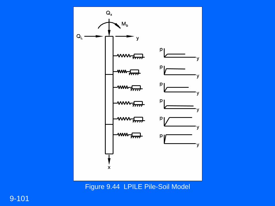
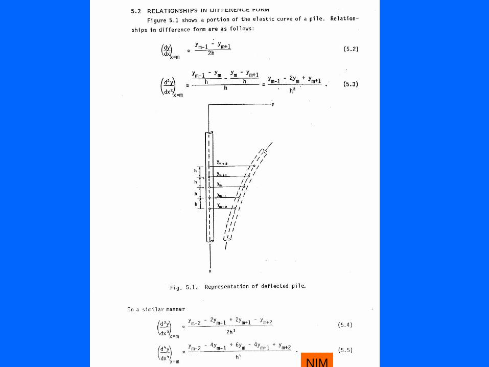
Figure 9.44 LPILE Pile-Soil Model

9-101

NIM

NIM

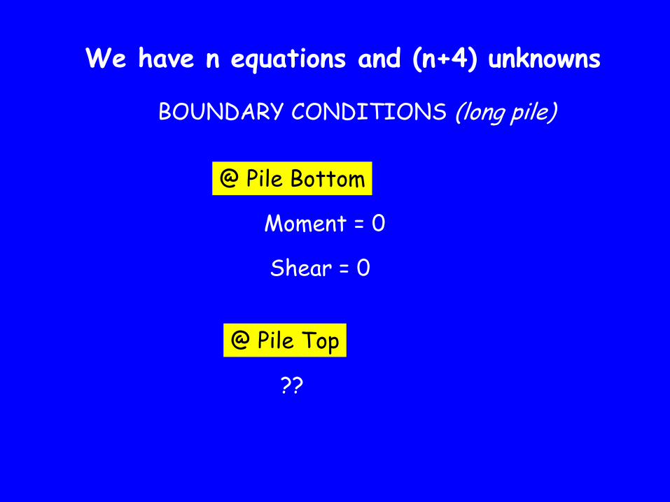
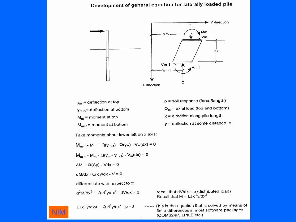
We have n equations and (n+4) unknowns

BOUNDARY CONDITIONS (long pile)

@ Pile Bottom

Moment = 0

Shear = 0

@ Pile Top

??

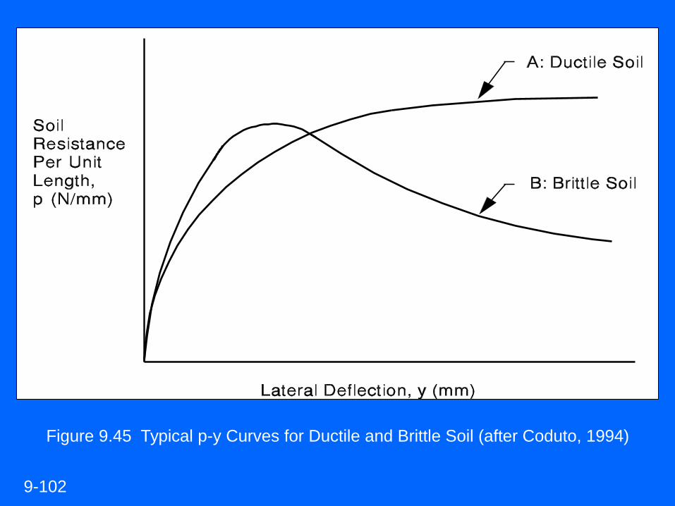
Figure 9.45 Typical p-y Curves for Ductile and Brittle Soil (after Coduto, 1994)

9-102

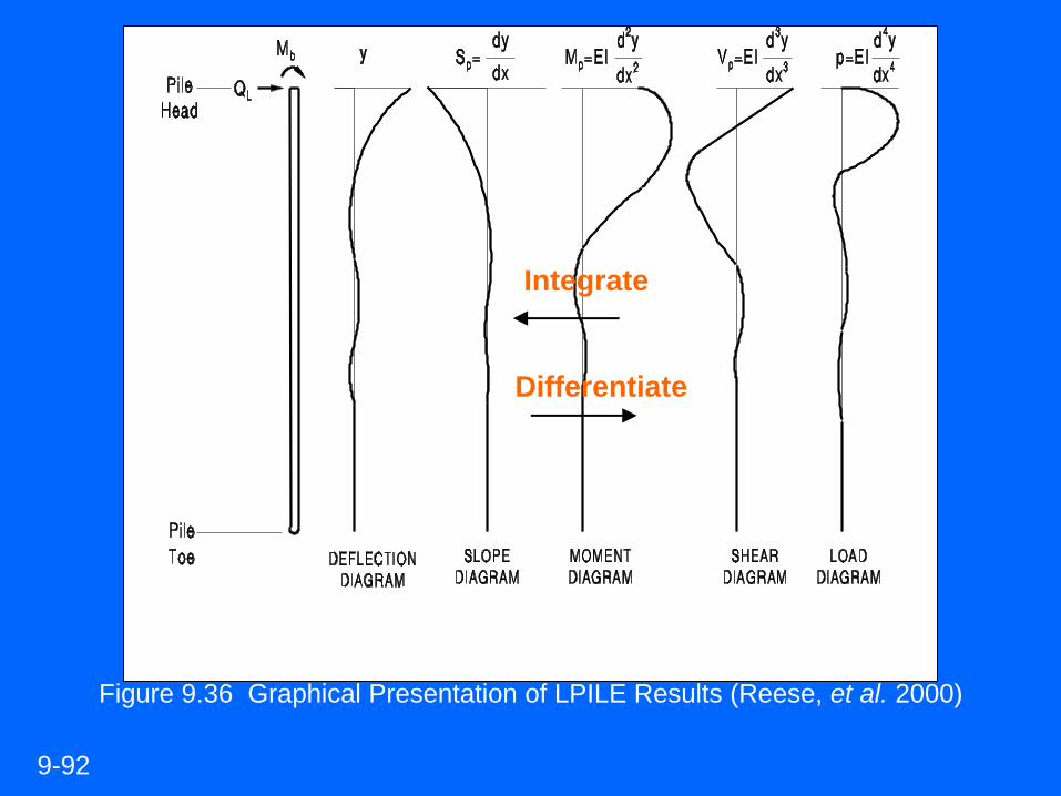
Figure 9.36 Graphical Presentation of LPILE Results (Reese, et al. 2000)

9-92

Differentiate

Integrate

LET’S EAT !!