Introduction to Real Analysis M361K - University of … · Preface These notes are for the basic real analysis class. (The more advanced class is M365C.) They were writtten, used,

Introduction to Real Analysis

M361K

Preface

These notes are for the basic real analysis class. (The more advanced class is M365C.)They were writtten, used, revised and revised again and again over the past five years.The course has been taught 12 times by eight different instructors. Contributors tothe text include both TA’s and instructors: Cody Patterson, Alistair Windsor, TimBlass, David Paige, Louiza Fouli, Cristina Caputo and Ted Odell.

The subject is calculus on the real line done the right way. The main topics aresequences, limits, continuity, the derivative and the Riemann integral. it is a challengeto choose the proper amount of preliminary material before starting with the maintopics. In early editions we had too much and decided to move some things into anappendix to Chapter 2 (at the end of the notes) and to let the instructor choose whatto cover. We also removed much of the topology on R materal from Chapter 3 andput it in an appendix. In a one semester course we are able to do most problems fromChapter 3–6 and a selection of certain preliminary problems from Chapter 2 and thetwo appendices.

March 2009

Contents

Chapter 1. Introduction 1

Chapter 2. Preliminaries: Numbers and Functions 51. The Absolute Value 82. Intervals 93. Functions 10

Chapter 3. Sequences 151. Limits 152. Archimedean Property 173. Convergence 184. Monotone Sequences; least upper bound

and greatest lower bound 205. Subsequences 236. Cauchy Sequences 247. Decimals 25

Chapter 4. Limits and Continuity 291. Limits 292. Continuous Functions 333. Uniform Continuity 36

Chapter 5. Differentiation 371. Derivatives 372. The Mean Value Theorem 39

Chapter 6. Integration 411. The Definition 412. Integrable Functions 433. Fundamental Theorems of Calculus 454. Integration Rules 46

Appendix. Appendix to Chapter 2 471. The Field Properties 472. The Order Properties 493. The Ordered Field Properties 504. Set Theory 525. Cardinality 53

iii

iv CONTENTS

6. Mathematical Induction 56

Appendix. Appendix to Chapter 3 571. Open and Closed Sets 572. Compactness 593. Sequential Limits and Closed Sets 60

CHAPTER 1

Introduction

Goals

The purpose of this course is three-fold:

(1) to provide an introduction to the basic definitions and theorems of real anal-ysis.

(2) to provide an introduction to writing and discovering proofs of mathematicaltheorems. These proofs will go beyond the mechanical proofs found in yourDiscrete Mathematics course.

(3) to experience the joy of mathematics; the joy of personal discovery.

Proofs

Hopefully all of you have seen some proofs before. A proof is the name that math-ematicians give to an explanation that leaves no doubt. The level of detail in thisexplanation depends on the audience for the proof. Mathematicians often skip stepsin proofs and rely on the reader to fill in the missing steps. This can have the ad-vantage of focusing the reader on the new ideas in the proof but can easily lead tofrustration if the reader is unable to fill in the missing steps. More seriously thesemissing steps can easily conceal mistakes; most mistakes in proofs begin with “it isclear that”.

In this course we will try to avoid missing any steps in our proofs; each statementshould follow from a previous one by a simple property of arithmetic, by a definition,or by a previous theorem, and this justification should be clearly stated. Writingclear proofs is a skill in itself. Often the shortest proof is not the clearest.

There is no mechanical process to produce a proof but there are some basic guidelinesyou should follow. The most basic is that every object that appears should be defined;when a variable, function, or set appears we should be able to look back and find astatement defining that object:

(1) Let ε > 0 be arbitrary.(2) Let f(x) = 2x+ 1.(3) Let A = {x ∈ R : x13 − 27x12 + 16x2 − 4 = 0}.(4) By the definition of continuity there exists a δ > 0 such that...

1

2 1. INTRODUCTION

Always watch out for hidden assumptions. In a proof, you may want to say “Letx ∈ A be arbitrary,” but this does not work if A = ∅ (the empty set). A commonerror in real analysis is to write lim

n→∞an or lim

x→af(x) without first checking whether the

limit exists (often this is the hardest part).

The audience for which a proof is intended is what determines how the proof iswritten. Your audience is another student in the class who is clueless as to how toprove the theorem.

Logic

We will avoid using logical notation in our definitions and statements of theorems.Instead we will use their English equivalents. Beyond switching to the contrapositiveand negating a definition, formal logical manipulation is rarely helpful in provingstatements in real analysis.

You should be familiar with the basic logical operators: if P and Q are propositions,i.e., statements that are either true or false, then you should understand what ismeant by

(1) not P(2) P or Q – the mathematical use of “or” is not exclusive so P or Q is true

even if both P and Q are true.(3) P and Q(4) if P then Q (or “P implies Q”)(5) P if and only if Q (sometimes written P is equivalent to Q)

Similarly if P (x) is a predicate, that is a statement that becomes a proposition whenan object such as a real number is inserted for x, then you should understand

(1) for all x, P (x) is true(2) there exists an x such that P (x) is true

Simple examples of such a P (x) are “x > 0” or “x2 is an integer.”

You should know the formulae for negating the various operators and quantifiers.

Most of our theorems will have the form of implications: “if P then Q.” P is calledthe hypothesis and Q the conclusion.

Definition. The contrapositive of the implication “if P then Q” is the implication“if not Q then not P .” The contrapositive is logically equivalent to the originalimplication. This means that one is valid (true) if and only if the other is valid.

Sometimes it is much easier to pass to the contrapostive formulation when provinga theorem.

Definition. The converse of the implication if P then Q is the implication if Qthen P . The converse is not logically equivalent to the original implication.

1. INTRODUCTION 3

Definition. A statement that is always true is called a tautology. An implicationthat is a tautology is called a valid argument. A statement that is always false iscalled a contradiction.

To show that an argument is not valid it suffices to find one situation in whichthe hypotheses are true but the conclusion is false. Such a situation is called acounterexample.

One technique of proof is by contradiction. To prove “P implies Q” we might assumethat P is true and Q is false and obtain a contradiction. This is really proving thecontrapositive.

CHAPTER 2

Preliminaries: Numbers and Functions

What exactly is a number?

If you think about it, to give a precise answer to this question is surprisingly difficult.As is often the case, the word ‘number’ reflects a concept of which we have someintuitive understanding, but no concrete definition. We will try to describe exactlywhat we should expect from a number system. These expectations will lead us toconclude that a number is an element of R, the collection of real numbers. Most ofus have probably heard of the real numbers, but may not be exactly sure what theyare.

In particular, we might ask: Why exactly are the real numbers so important? Is theresome other system that would also suffice to be our system of numbers? What iswrong with just using the natural numbers, the integers, or the rational numbers? Toanswer this question, we will have to pin down the expectations we have on a numbersystem. More precisely, we will have to decide exactly what properties should holdin a system of numbers. It is actually not so difficult to make progress in this area:it only requires a little bit of introspection and memory.

Think back to when you first met the idea of a number. Probably the very firstpurpose of a number in your life is that it allowed you to count things: 50 states,32 professional football teams, 7 continents, 5 golden rings, etc. Needing to countthings leads us to the invention (or discovery depending on your point of view) ofthe natural numbers (the numbers 1, 2, 3, 4, 5, · · · ). Mathematicians typically denotethe collection of natural numbers by the symbol ‘N.’ Though this collection canbe constructed quite rigorously from the standard axioms of mathematics, we willassume that we are all familiar with the natural numbers and their basic properties(such as the concept of mathematical induction; see appendix to Chapter 2). Thenatural numbers fulfill quite successfully our goal of being able to count.

The next thing that will expect of our number system is that it should be able toanswer questions like the following: “If the Big Twelve has 12 football teams andthe Big Ten has 11 (shockingly it’s true), how many teams do the conferences havebetween them?” In other words we will need to add. We will also multiply. Thenatural numbers are already well-suited for these tasks. Really this should not comeas a surprise. After all, adding is really just a different way of looking at counting (i.e.,

5

6 2. PRELIMINARIES: NUMBERS AND FUNCTIONS

adding three and five is the same as taking three dogs and five cats and counting thetotal number of animals). As we all know, multiplication is really repeated addition.

Having addition naturally leads us to subtraction. This is the first place the naturalnumbers will fail us. Subtracting 7 from 2 is an operation that cannot be performedwithin N. The need for subtraction, therefore, is one of the reasons that N will notwork as our entire number system. Thus we are lead to expand to the integers.As we all probably know, the integers are comprised of the natural numbers, thenumber zero, and the negatives of the natural numbers (at this point, you mightprotest and say that zero should be included as a natural number as it allows us tocount collections which contain no objects; in fact many mathematicians do includezero in N, but the distinction is of little importance). The collection of integers isdenoted by Z. Again we will assume we know all the basic properties of Z (like primefactorization).

The integers are a very good number system for most purposes, but they still havean obvious defect: we cannot divide. Surely any reasonable number system allowsdivision. If you and I have a sandwich and we each want an equal share, how much dowe each get? Needing division, we throw in fractions: symbols which are comprisedof two integers, one in the numerator and one in the denominator (of course thedenominator is not allowed to be zero). A fraction will represent the number whichresults when the numerator is divided by the denominator. Things start to get a littlebit complicated here. We can now have more than one symbol that that stand forthe same number: 2

2and 1

1will both stand for integer 1.

Combining all the numbers we have so far gives Q, the collection of rational numbers.Again, we will assume that we are familiar with all its basic properties. Before we goon to justify our assertion that Q is not a sufficient number system, we have anotherproperty to point out. Notice that most of our properties so far involve operationsamong our numbers: namely addition, subtraction, multiplication, and division. Wecall these types of properties algebraic (In mathematics, the word algebra describesthe study of operations). The property we are going to discuss next is not algebraic.

Suppose then that I pick a rational number and you pick another. We can easilydecide which is bigger: Namely a

bis bigger than c

d(where a, b, c, and d are integers)

if ad is bigger than bc (assuming b and d both positive; we can easily assure bothdenominators are positive by moving any negative into the numerator). Since ad andbc are integers, we know how to compare them (because we know how to comparenatural numbers and how to take negatives into account). Since we can alwayscompare any two rational numbers in this way, we say that Q is totally ordered.

In retrospect, we should have demanded this property of our number system from thebeginning. Numbers should come with some notion of size. Fortunately, we got itfor free. Moreover, it is interesting to notice that the our expectation that a numbersystem should include the natural numbers and that it should have certain algebraicproperties is enough to lead us to include all of Q. We did not to request that our

2. PRELIMINARIES: NUMBERS AND FUNCTIONS 7

system be ordered to find Q. The order properties turn out to be more importantin telling us which potential numbers we should NOT include (such as the imaginarynumber i).

Q comes very close to satisfying everything we want in a number system. Unfortu-nately it is still lacking. Suppose we draw a circle whose diameter is 1. The lengtharound the circle (usually called the circumference) should certainly be a number.If, however, we restrict ourselves to the rational numbers, this length will not be anumber (the number is of course usually denoted π and it is not a rational number).The same could be said of the length of one of the sides of a square whose area is 2(this number is usually denoted

√2).

These two examples merely comprise our attempt to give (geometric) demonstrationthat Q is lacking as a number system. The real (more general) property that weseek, called completeness , is actually quite subtle and has to do with the presenceof something like ‘gaps’ in Q (the absence of the number

√2 or the number π is

an example of such a gap). These gaps have to do with something called a Cauchysequence which we will study in detail in this course. One consequence of filling inthese gaps is that we are able to perform calculus. This, in turn, allows us to expressall the lengths (and areas, volumes, etc.) of geometric objects like the examples aboveas real numbers.

One of the fundamental results in mathematics is that the collection of real numbersis the ONLY system of numbers which satisfies all of our demands. We will formulateour demands precisely throughout the first three sections of this chapter with theexception of the completeness axiom). We are thus forced to admit that the realnumbers comprise the only possible choice of a number system. To give an exactdefinition of the real number is surprisingly complicated. In fact, the first rigorousconstruction of the real numbers was given by Georg Cantor as late as 1873 (bycomparison, the rational numbers where constructed in ancient times).

For our purposes, we will take it on faith that the real numbers exist as a numbersystem. In the appendix to this chapter, we will state precisely the important prop-erties of the real numbers (which we will also take on faith) and note that these lineup with our expectations of the number system (except for the completeness axiomwhose importance might not be clear at first; keep our geometric example in mind).In the next chapter, we will also describe a way to define the real numbers rigorouslyusing decimal expansions (there are actually several well-known ways).

Finally, it is important to realize that the properties given in the appendix (whichwe will call axioms), together with the completeness axiom, are the ONLY propertiesthat we assume about R. Strictly speaking, any other statement we want to makemust be proven from either from our axioms or from properties we have alreadyassumed about N, Z, and Q (or, of course, some combination of the two).

In general, however, this can get to be a little bit tedious. Hence we will allow you toassume all of the ‘basic’ or ‘obvious’ properties of the real numbers. Unfortunately,


deciding which properties are obvious is a subjective process. Therefore, if there isany doubt about whether a statement is obvious, you should prove it rigorously fromthe axioms (or at least describe how to prove it rigorously). Actually, the ability todecide when statements are obvious or ‘trivial’ is an important skill in mathematics.Possessing this ability can often be a reflection of great mathematical maturity andinsight.

In the appendix to this chapter, we will also derive some properties of R that followfrom our axioms. We will work on some of these in class, but thereafter you mayconsider them “known.” The appendix also contains a discussion of basic set theoryand induction.

1. The Absolute Value

An important property of the real numbers is that we can define a size on them,which we call the absolute value. The definition is relatively simple and yet it hasvast and important consequences.

Definition. Given a real number a ∈ R, we define the absolute value of a, denoted|a| to be a if a is nonnegative and −a if a is negative.

2.1. For a ∈ R: 1) |a| ≥ 0, 2) |a| = 0 if and only if a = 0, and 3) |a| ≥ a.

The following technical observations will be of assistance in some arguments involvingthe absolute value.

2.2. For all a ∈ R, a2 = |a|2.2.3. For all a, b ∈ R with a, b ≥ 0 we have a2 ≤ b2 if and only if a ≤ b. Likewise,a < b if and only if a2 < b2.

The next statement gives two fundamental properties of the absolute value.

2.4. Let a, b ∈ R, then

(1) |ab| = |a||b| and(2) |a+ b| ≤ |a| + |b|

Hint: One can prove these by laboriously checking all the cases (e.g., a > 0, b ≤ 0)but in each case an elegant proof is obtained by using our observations to eliminatethe absolute value and then proceeding using the properties of arithmetic.

The second inequality above is perhaps the most important inequality in all of anal-ysis. It is called the triangle inequality.

The remaining results in this section are important consequences of the triangle in-equality.

2.5. Let a, b, c ∈ R. Then we have

2. INTERVALS 9

(1) |a− b| ≥ ∣∣|a| − |b|∣∣ and(2) |a− c| ≤ |a− b| + |b− c|.

You have probably measured the length of something using a yardstick. You mightplace one end at zero and see where the other end lies to get the length. In a tightplace you might place the yardstick and find one end at 7′′ and other at 13′′ andconclude the length is 13′′ − 7′′ = 6′′. If I told you one end was at x and the otherwas at y, what would be the length? Well, y−x if y > x and x− y if x > y. In short,it would be |x− y|. So, we can regard |x− y| as the distance between the numbersx and y. Note this works for all real numbers, even if one or both is negative. Notethat this explains why (see 2.5(2)) we call 2.4(2) the triangle inequality.

2.5(1) is often called the reverse triangle inequality.

2.6. Let x, ε ∈ R with ε > 0. Then we have the following two statements.

(1) |x| ≤ ε if and only if −ε ≤ x ≤ ε. The double inequality −ε ≤ x ≤ ε means−ε ≤ x and x ≤ ε.

(2) If a ∈ R, |x− a| ≤ ε if and only if a− ε ≤ x ≤ a+ ε.

Remark. By a similar proof, the same properties hold with ≤ replaced by <.

2. Intervals

Intervals are a very important type of subset of R. Loosely speaking they are setswhich consist of all the numbers between two fixed numbers, called the endpoints. Wealso (informally) allow the endpoints to be ±∞. Depending on whether the endpointsare finite and whether we include them in our sets, we arrive at 9 different types ofintervals in R.

Definition. An interval is a set which falls into one of the following 9 categories(assume a, b ∈ R with a < b). We apply the word ‘bounded’ if both the endpointsare finite. Otherwise we use the word ‘unbounded’.

(1) Bounded open intervals are sets of the form

(a, b) := {x ∈ R : a < x < b}.(2) Bounded closed interval are sets of the form

[a, b] := {x ∈ R : a ≤ x ≤ b}.(3) There are two type of half-open bounded intervals. One type is sets of the

form

[a, b) := {x ∈ R : a ≤ x < b}.(4) The other is sets of the form

(a, b] := {x ∈ R : a < x ≤ b}.


(5) There are also two types of unbounded open intervals not equal to R. Onetype is sets of the form

(a,+∞) := {x ∈ R : a < x}.(6) The other is sets of the form

(−∞, b) := {x ∈ R : x < b}.(7) There are two types of unbounded closed intervals not equal to R. One type

is sets of the form

[a,+∞) := {x ∈ R : a ≤ x}.(8) The other is sets of the form

(−∞, b] := {x ∈ R : x ≤ b}.(9) The whole real line R = (−∞,∞) is an interval. We count R as being open,

closed, and unbounded.

Some authors include the empty set, ∅, and single points, {a} for some a ∈ R,as intervals. To distinguish these special sets, people often call them ‘degenerateintervals’ whereas sets of the above would be ‘nondegenerate invervals.’ We willreserve the word ‘interval’ for the nondegenerate case. That is, in our language, aninterval is not allowed to be ∅ or {a}.Definition. The closure of an interval I, denoted I, is the union of I and it endpoints.

Thus

(a, b) = [a, b] = [a, b) = (a, b] = [a, b]

(a,+∞) = [a,+∞) = [a,+∞)

(−∞, b) = (−∞, b] = (−∞, b]

R = R

Definition. The interior of an interval I, denoted I◦, is I minus its endpoints.

Thus

(a, b)◦ = [a, b]◦ = [a, b)◦ = (a, b]◦ = (a, b)

(a,+∞)◦ = [a,+∞)◦ = (a,+∞)

(−∞, b)◦ = (−∞, b]◦ = (−∞, b)

R◦ = R

3. Functions

Even more basic to mathematics than the concept of a number is the concept of afunction. Roughly speaking, a function f from a set A to a set B is a rule that assigns

3. FUNCTIONS 11

to each x ∈ A an element f(x) ∈ B. In this case we write f : A → B. What do wemean by “rule”? Let’s try to be more precise.

Definition. A function f from A to B, denoted by f : A→ B, is a subset f of theCartesian product A× B = {(a, b) : a ∈ A, b ∈ B} satisfying

(1) for each a ∈ A there exists b ∈ B such that (a, b) ∈ f(2) for all a ∈ A and for all b, b′ ∈ B if (a, b) ∈ f and (a, b′) ∈ f then b = b′.

We could combine the two hypotheses into a single statement:

for each a ∈ A there exists a unique b ∈ B such that (a, b) ∈ f

Rather than writing (a, b) ∈ f it is customary to write f(a) = b.

Technically then a function from A to B is just a special subset of A×B. Mathemati-cians, however, rarely think of functions in this way. The idea of a rule is intuitivelymore accurate whereas the formal definition is just a way to make it precise.

It is very important to realize that a function is not the same thing as a formula.Many beginning students in mathematics think that in order to find a function, theyneed to find a formula using variables. This is not the case. It is perfectly reasonableto define a function by saying something like:

Define a function from the set of real numbers to the set {0, 1} byassigning the value 1 to all rational numbers and the value 0 to allirrational numbers.

Since every number has been given a value and no number has been given more thenone, our rule gives a function.

This function f : R → {0, 1} would probably be more commonly described by sayingthat for x ∈ R,

f(x) =

⎧⎨⎩

1 if x ∈ Q

0 if x ∈ R\Q

,

but either description would work. Notice that it would be impossible to find whatmost people would call a ‘formula’ to describe this function.

Definition. Let f : A→ B be a function. The set A is called the domain of f andB is called the co-domain.

The range of f , denoted by f(A), is

f(A) = {f(a) : a ∈ A}.Most of the functions we consider will be of the form f : R → R or f : A→ R whereA ⊆ R.


A function is sometimes called a mapping or a transformation. If f(a) = b wemight say “f maps a to b” or “f sends a to b.” Some functions have certain specificproperties that we shall name.

Definition. Let f : A→ B.

(1) f is onto (or surjective) if f(A) = B. That is, f is onto if, for every b ∈ B,there exists some a ∈ A such that f(a) = b.

(2) f is 1–1 (or one-to-one or injective) if for all a1, a2 ∈ A, f(a1) = f(a2)implies a1 = a2. That is, f is 1–1 if, for all a1, a2 ∈ A such that a1 = a2, wehave f(a1) = f(a2).

(3) f is a bijection (or 1–1 correspondence) if it is 1–1 and onto. This isequivalent to: for all b ∈ B there exists a unique a ∈ A with f(a) = b. (Note:it is usually simpler to show that a function is a bijection by showing it is1–1 and onto separately.)

If a function is a bijection then you can “reverse it” to obtain a function going theother way. The following theorem makes this precise.

Theorem 2.7. Let f : A → B be a bijection. Then there exists a bijectiong : B → A satisfying

(1) for all a ∈ A, g(f(a)) = a.(2) for all b ∈ B, f(g(b)) = b.

Furthermore, this function g is unique; if g1 and g2 are bijections satisfying (1) and(2) then g1 = g2. (Would it be enough to assume g1 and g2 both satisfy (1)?)

The bijection g is called the inverse function of f and is usually denoted by f−1.Do not confuse this with “1/f”.

Definition. Let f : A→ B. Let D ⊆ A, and C ⊆ B.

(1) The image of D under f , denoted f(D), is

f(D) = {f(x) : x ∈ D}.(2) The pre-image, of C under f , denoted f−1(C), is

f−1(C) = {a ∈ A : f(a) ∈ C}.The set f−1(C) always exists even when the function f−1 does not exist. The contextof a problem will tell you which “f−1” is being used.

We are using the symbol f−1 in two different ways. When the function f−1 doesexist then there are two different ways of reading f−1(C); it can be read as the directimage of the set C under the function f−1 or it can be read as the inverse image ofC under the function f . These give the same set and thus there is no ambiguity, inthis case.

3. FUNCTIONS 13

Definition. Let f : A → B and g : B → C. The composition g ◦ f : A → C isdefined by (g ◦ f)(a) = g(f(a)).

2.8. Let f : A→ B and g : B → C be two bijections. Then g ◦ f : A→ C is also abijection.

Caution: If f and g are functions, it is not true in general that f ◦ g = g ◦ f . Infact, these two compositions may have completely different domains and co-domains!

Note: If f : A → B is a bijection then f−1 ◦ f : A → A is the identity map on Aand f ◦ f−1 : B → B is the identity map on B. (The identity map on the set S is themap id : S → S defined by id(x) = x for all x ∈ S.)

CHAPTER 3

Sequences

1. Limits

Our basic object for investigating real analysis will be the sequence.

Definition. A sequence in R is a function f : N → R.

Example. f(n) = n2 and g(n) =√n both define sequences in R.

We typically do not use functional notation to discuss sequences, instead we writethings like (n2)∞n=1 or (

√n )∞n=1. If we say “Consider the sequence (an)∞n=1,” we are

referring to the sequence whose value at n is an. Sequences, like general functions,can be defined without using an explicit formula.

Example. We can define a sequence (an)∞n=1 by

an = nth digit to right of the decimal point for π.

Thus (an)∞n=1 = (1, 4, 1, 5, 9, . . .).

Example. We can define a sequence recursively; that is using the previous membersof the sequence to define the next element. A famous example of a recursively definedsequence is the Fibonacci sequence given by

a1 = 1 a2 = 1 an+2 = an+1 + an for n ≥ 1.

Find a3, a4, a5.

A sequence is not to be confused with a set. For example {1, 1, 1, . . .} = {1} but(1, 1, 1, . . .) denotes f : N → R with f(n) = 1 for all n. This is an example of aconstant sequence. A sequence is really an infinite ordered list of real numbers,which may repeat.

Remark. Sometimes we will write “consider the sequence (an)∞n=4.” Of course thisis given by f(n) = a3+n for n ∈ N so it is a sequence even though for convenience orwhatever reason we chose to “start the sequence at n = 4.”

Intuitively a sequence (an)∞n=1 converges to a limit L if the terms get closer and closerto L as n gets larger and larger.

Now we need to make this idea precise so we can use it in our future discussions.First note that (1, 0, 1

2, 0, 1

3, 0, . . .) should converge to 0 under our yet to be formulated

15

16 3. SEQUENCES

definition. But it is not true that each term is closer to 0 than the previous term. Sothe rough intuitive “definition” needs clarification.

The following definition makes this intuition precise:

Definition. A sequence (an)∞n=1 is said to converge to L ∈ R if for all ε > 0 thereexists N ∈ N so that for all n ≥ N , |an − L| < ε. L is called a limit of the sequence(an)∞n=1. If there exists an L ∈ R such that (an)∞n=1 converges to L then we say (an)∞n=1

converges or (an)∞n=1 is a convergent sequence.

Note: It is important to realize that the N that you choose will typically depend onε. Typically we expect that N will get larger as ε gets closer to 0.

This definition seems to have been first published by Bernard Bolzano, a Czech math-ematician, in 1816. It is the notion of limit that distinguishes analysis/calculus from,say, algebra. This definition came about 150 years after the creation of calculus (dueindependently to Newton and Leibniz). The fact that it will probably take you sometime to understand and become happy with it is therefore no surprise. The old guyswere pretty sharp and still struggled with the notion.

Lemma 3.1. Let a ≥ 0 be a real number. Prove that if for every ε > 0 we have thata < ε then a = 0.

3.2. Prove that if (an)∞n=1 converges to L ∈ R and (an)∞n=1 converges to M ∈ R thenL = M . (Hint: argue by contradication.)

We have just shown if a sequence has a limit then that limit is unique. Thus it makessense to talk about the limit of a sequence and to write lim

n→∞an = L.

Caution: Before we write limn→∞

an we must know that an has a limit.

3.3. Negate the definition of limn→∞

an = L to give an explicit definition of “(an)∞n=1

does not converge to L.”

Remark. We can write (an)∞n=1 does not converge to L as (an)∞n=1 → L.

Caution: We should not write limn→∞

an = L to mean (an)∞n=1 does not converge to L

unless we know that limn→∞

an exists.

Definition. A sequence (an) is said to diverge if it does not converge to L for anyL ∈ R. We will distinguish two special types of divergence:

(1) A sequence (an) is said to diverge to +∞ if for all M ∈ R there existsN ∈ N such that for all n ≥ N we have an ≥M . In an abuse of notation weoften write lim

n→∞an = +∞.

(2) A sequence (an) is said to diverge to −∞ if for all M ∈ R there existsN ∈ N such that for all n ≥ N we have an ≤M . In an abuse of notation weoften write lim

n→∞an = −∞.

2. ARCHIMEDEAN PROPERTY 17

3.4. Prove that a sequence (an)∞n=1 converges to L ∈ R if and only if for all ε > 0 theset

{n ∈ N : |an − L| ≥ ε}is finite. This is saying that the number of terms an which are more than ε distancefrom L must be finite.

This has a couple of interesting corollaries;

(1) if we change finitely many terms of a sequence we do not alter its limitingbehaviour; if the sequence originally converged to L then the altered sequencestill converges to L, and if the original sequence diverged then so does thealtered sequence.

(2) if we remove a finite number of terms from a sequence then we do not alter itslimiting behaviour; if the sequence originally converged to L then the alteredsequence sequence still converges to L, and if the original sequence divergedthen so does the altered sequence.

3.5. Prove using the definition of a limit that limn→∞

1n

= 0.

Let’s examine the proof here. Your proof should look something like this.

Proof. We will show limn→∞

1n

= 0. Let ε > 0 be arbitrary but fixed. We must find

N ∈ N so that if n ≥ N then | 1n− 0| < ε which is the same as 1

n< ε. Choose N ∈ N

so that 1N< ε. Then if n ≥ N , 1

n≤ 1

N< ε. �

We have used here two things. First the basic properties of order which we willassume you know. Secondly, we have used that: given ε > 0 there exists N ∈ N with1N< ε or in other form, 1

ε< N . This is called the Archimedian property.

2. Archimedean Property

R has the Archimedean Property, which says that for every x there exists ann ∈ N with x < n. This seemingly innocuous property has many consequences:

(1) For every ε > 0 there exists an n ∈ N such that

0 <1

n< ε,

(2) for every x ∈ R there exists an m ∈ Z such that

m ≤ x < m+ 1,

(3) for every x ∈ R and n ∈ N there exists an m ∈ Z such that

m

n≤ x <

m+ 1

n,

18 3. SEQUENCES

3.6. Using these we can prove that every real number can be approximated arbitrarilywell by a rational number. We say that Q is dense in R.

(1) Prove that for every x ∈ R and every ε > 0 there exists mn∈ Q such that

0 ≤ x− m

n< ε.


−ε < x− m

n≤ 0

Similarly, the irrational numbers are dense in R.

3.7. Prove:

(1) For all mn∈ Q \ {0} the number

√2 m

nis irrational.


0 ≤ x−√

2m

n< ε.


−ε < x−√

2m

n≤ 0

3. Convergence

3.8. Prove using the definition of a limit that a) limn→∞

1− 1n2+1

= 1, b) limn→∞

n2−12n2+3

= 12.

3.9. Prove or disprove: To disprove you need only give a counterexample.

(1) If limn→∞

an = L then limn→∞

|an| = |L|.(2) If lim

n→∞|an| = |L| then lim

n→∞an = L.

(3) If limn→∞

|an| = 0 then limn→∞

an = 0.

(4) If an ≤ cn ≤ bn for all n ∈ N and limn→∞

an = limn→∞

bn = L then limn→∞

cn = L.

This is normally referred to as the Squeeze Theorem for sequences.

Definition. A sequence (an)∞n=1 is called bounded if the set {an : n ∈ N} iscontained in a bounded interval.

Note: Thus (an) is bounded if and only if there exists K ≥ 0 with |an| ≤ K for alln ∈ N.

3.10. Prove that if (an)∞n=1 is a convergent sequence with limn→∞

an = L then (an)∞n=1 is

bounded. Is the converse true?

We can now justify our use of the word “diverges” in the situation that a sequencegoes to ±∞.

3. CONVERGENCE 19

3.11. Show that if (an) diverges to ∞ then an diverges. Show that if (an) divergesto −∞, it also diverges.

3.12. Let (bn)n=1∞ be a convergent sequence with limn→∞

bn = M with M = 0. Prove

that there exists an N ∈ N such that for all n ≥ N we have |bn| > |M |2

.

The following are often called the “Limit Laws” for sequences.

3.13. Let (an)∞n=1 and (bn)∞n=1 be sequences and c ∈ R be an arbitrary real number.We can define new sequences (c · an)∞n=1, (an + bn)∞n=1, and (an · bn)∞n=1. If bn = 0 for

all n ∈ N then we can define(an

bn

)∞n=1

.

Prove that:

(1) If (an)∞n=1 is a convergent sequence and c ∈ R then (c · an)∞n=1 is a convergentsequence and

limn→∞

(c · an) = c · limn→∞

an.

(2) If (an)∞n=1 and (bn)∞n=1 are convergent sequences then (an + bn)∞n=1 is a con-vergent sequence and

limn→∞

(an + bn) = limn→∞

an + limn→∞

bn.

(3) If (an)∞n=1 and (bn)∞n=1 are convergent sequences then (an · bn)∞n=1 is a conver-gent sequence and

limn→∞

(an · bn) =(

limn→∞

an

) · ( limn→∞

bn).

(4) If (an)∞n=1 and (bn)∞n=1 are convergent sequences with bn = 0 for all n ∈ N

and limn→∞

bn = 0 then

limn→∞

an

bn=

limn→∞ an

limn→∞ bn.

Hint for (3): The problem in (3) is that we have two quantities changing simultane-ously. To deal with this we use a very common trick in analysis: we add and subtractadditional terms, which does not affect the value, and then group terms so that eachterm is a product of things we can control. Let L = lim

n→∞an and M = lim

n→∞bn. We can

write

an · bn − L ·M = an · bn − L ·M + L · bn − L · bn= (an − L) · bn + L · (bn −M).

Hint for (4): Given (3) it suffices to prove (explain why) that

limn→∞

1

bn=

1

limn→∞

bn.

20 3. SEQUENCES

Let M = limn→∞

bn and notice that∣∣∣ 1

bn− 1

M

∣∣∣ =|M − bn||Mbn| <

|M − bn|(M2/2)

if |bn| > |M |2

. Now use Problem 3.12.

3.14. Suppose a ≤ an ≤ b for all n ∈ N. Prove that if limn→∞

an = L, then L ∈ [a, b].

3.15. Let (an)∞n=1 and (bn)∞n=1 be convergent sequences with a = limn→∞

an and b =

limn→∞

bn. Prove that if an − bn = 1n

for all n ∈ N then a = b. Would this theorem still

be true if, instead of equality, you had an − bn <1n? What if an − bn = 1

2n ?

4. Monotone Sequences; least upper boundand greatest lower bound

In general it can be difficult to show that a sequence converges. For certain classesof sequences checking for convergence can be much easier.

Definition. Let (an) be a sequence. We say

(1) (an) is increasing if for all n ∈ N, an ≤ an+1.(2) (an) is decreasing if for all n ∈ N, an ≥ an+1.(3) (an) is monotone if it is increasing or decreasing.

Before proceeding we need some new definitions.

Definition. Let A ⊆ R and x ∈ R.

(1) x is called an upper bound for A if, for all a ∈ A, we have a ≤ x.(2) x is called an lower bound for A if, for all a ∈ A, we have x ≤ a.(3) The set A is called bounded above if there exists an upper bound for A.

The set A is called bounded below if there exists a lower bound for A. Theset A is called bounded if it is both bounded above and bounded below.

(4) x is called a maximum of A if x ∈ A and x is an upper bound for A.(5) x is called a minimum of A if x ∈ A and x is a lower bound for A.

In (4) ((5)) we write x = maxA (minA). Note there is only one maximum (orminimum), if any.

3.16. For each of the following subsets of R:

(a) A = ∅,(b) A = {a ∈ R : 0 < a ≤ 1},(c) A = {a ∈ R : 2 ≤ a}.(d) A = {a ∈ R : a2 < 2},(1) Find all lower bounds for A and all upper bounds for A,

4. MONOTONE SEQUENCES; LEAST UPPER BOUND AND GREATEST LOWER BOUND 21

(2) Find minA and maxA if they exist.(3) Discuss whether A is bounded.

Definition. Let A ⊆ R and x ∈ R

(1) x is called a least upper bound of A or supremum of A if(a) x is an upper bound for A,(b) if y is an upper bound for A then x ≤ y.

(2) x is called a greatest lower bound of A or infimum of A if(a) x is a lower bound for A,(b) if y is a lower bound for A then y ≤ x.

3.17. Let A ⊆ R. Prove that if x is a supremum of A and y is a supremum of A thenx = y.

Hence, if the set A has a supremum then that supremum is unique and we can speakof the supremum of A and write supA. Similarly, if the set A has an infimum thenthat infimum is unique and we can speak of the infimum of A and write inf A.

3.18. Find inf A and supA, if they exist, for each of the following subsets of R:

(a) A = ∅,(b) A = {a ∈ R : 0 < a ≤ 1},(c) A = {a ∈ R : 2 ≤ a}.(d) A = {a ∈ R : a2 < 2},

The above definitions could also be made in Q or in any other subset of R. Ofcourse the answers to the exercises would depend upon the universe in question. Forexample if A is the set of all positive irrationals, then inf A would not exist inside ofthe universe R \ Q.

The Completeness Axiom: R is complete. That is, if A ⊆ R, A = ∅ and A isbounded above, then supA exists.

Though supA need not be in the set A there are elements of A arbitrarily close tosupA.

3.19. Let A ⊆ R be non-empty and bounded above. Prove that if s = supA thenfor every ε > 0 there exists an a ∈ A with s− ε < a ≤ s.

What would the equivalent property of inf A be?

3.20. Let A ⊆ R be bounded above and non-empty. Let s = supA. Prove that thereexists a sequence (an) ⊆ A with lim

nan = s. Prove that, in addition, the sequence

(an) can be chosen to be increasing, i.e., an ≤ an+1 for all n ∈ N.

What would be the analogous results for t = inf A, if A is bounded below?

22 3. SEQUENCES

3.21. Let A ⊆ R. Define

−A = {−x : x ∈ A}.(1) Prove that x is an upper bound for A if and only if −x is a lower bound for

−A.(2) Prove that x = supA if and only if −x = inf −A.(3) Prove that if A is non-empty and bounded below then inf A exists.

3.22. Prove or disprove:

(1) If A,B ⊆ R are nonempty sets such that for every a ∈ A and for every b ∈ Bwe have a ≤ b then supA and inf B exist and supA ≤ inf B.

(2) If A,B ⊆ R are nonempty sets such that for every a ∈ A and for every b ∈ Bwe have a < b, then supA and inf B exist and supA < inf B.

3.23. Let A,B ⊂ R be non-empty, bounded sets. We define A+B = {a+ b : a ∈ Aand b ∈ B}. Prove that

sup(A+B) = sup(A) + sup(B) and

inf(A+B) = inf(A) + inf(B)

3.24. Let f : R → R and g : R → R and A ⊆ R. Assume that f(A) and g(A) arebounded. Prove that

sup(f + g)(A) ≤ sup f(A) + sup g(A) .

Give examples where one has “=” and also “<”. State the analogous results for “inf”.

3.25. Prove the following:

(1) If (an) is increasing and unbounded then (an) diverges to +∞.(2) If (an) is decreasing and unbounded then (an) diverges to −∞(3) Let (an) be increasing and bounded. Let L = sup{an : n ∈ N}. Then

limn→∞

an = L.

(4) Let (an) be decreasing and bounded. Let L = inf{an : n ∈ N}. Thenlim

n→∞an = L.

3.26. Let A ⊂ R be a non-empty, bounded set. Let α = sup(A) and β = inf(A), andlet (an)∞n=1 ⊂ A be a convergent sequence, with a = lim

n→∞an. Prove that β ≤ a ≤ α.

Notice that a need not be equal to either of α or β, even if (an) is strictly increasingor strictly decreasing. For example, let A = [0, 1] so α = 1 and β = 0, and letan = 1

2+ 1

2n . Then (an) is strictly decreasing and a = limn→∞

an = 12. If, instead,

an = 12− 1

2n , then (an) would be strictly increasing and a = limn→∞

an = 12. In both

cases, a = α and a = β. Come up with a different example where (an) is monotonic(i.e., increasing or decreasing) but its limit is not α or β.

5. SUBSEQUENCES 23

3.27. If A ⊂ R is a non-empty, bounded set and B ⊂ A, prove

inf(A) ≤ inf(B) ≤ sup(B) ≤ sup(A) .

3.28. If A,B ⊂ R are both non-empty, bounded sets, prove

sup(A ∪ B) = max{sup(A), sup(B)} .

3.29. We analyze the important sequence (rn)∞n=1, where r ∈ R.

(1) Prove that if 0 ≤ r < 1 then (rn)∞n=1 converges to 0.Hint: Show the sequence is decreasing. Proceed by contradiction; supposeL = inf{an : n ∈ N} > 0, find an with L ≤ an < r−1L, and hence produce acontradiction.

(2) Prove that if r > 1 then (rn)∞n=1 diverges to +∞.(3) Use Problem 3.9 to complete the proof of the following fact: The sequence

(rn) converges if and only if −1 < r ≤ 1. If r = 1 then limn→∞

rn = 1. If

−1 < r < 1 then limn→∞

rn = 0.

The following example illustrates how powerful monotonicity is.

3.30. Let a1 = 2 and let (an) be generated by the recursive formula

an+1 =1

2

(an +

2

an

)for n ≥ 1.

(1) Prove that√

2 < an for all n ∈ N.Hint: Assuming an > 0 turn 1

2

(an + 2

an

)>

√2 into an equivalent condition

on a quadratic polynomial. Proceed by induction.(2) Prove that (an) is decreasing and hence converges.(3) Now take limits on both sides of the recursive formula using Problem 3.13

and use the fact that

limn→∞

an+1 = limn→∞

an

to find limn→∞

an.

Let x ∈ R+. What can you say about the sequence given by a1 = 1 and an+1 =12(an + x

an) for n ≥ 1?

5. Subsequences

If we have a sequence (an), a subsequence is a (new) sequence formed by skipping(possibly infinitely many) terms in an.

Definition. A sequence (bk)∞k=1 is a subsequence of (an)∞n=1 if there exists a strictly

increasing sequence of natural numbers n1 < n2 < · · · so that for all k ∈ N, bk = ank.

24 3. SEQUENCES

Example. (1, 1, 1, . . .) is a subsequence of (1,−1, 1,−1, . . .). In fact any sequence of±1’s is a subsequence of (1,−1, 1,−1, . . .).

In particular we see that a subsequence of a divergent sequence may be convergent.

Example. ( 1n2 )

∞n=1 is a subsequence of ( 1

n)∞n=1.

Both(

1n

)∞n=1

and(

1n2

)∞n=1

converge to 0.

3.31. Prove or disprove: If (bn) is a subsequence of (an) and limn→∞

an = L, then

limn→∞

bn = L.

Now we can play a fun game to see whether we can find subsequences with betterproperties than the original sequence.

3.32. Prove that every sequence of real numbers has a monotone subsequence.

Hint: Consider two cases. The first is the case in which every subsequence has aminimum element. In this case we can extract an increasing subsequence.

3.33. Let (xn)∞n=1 be an increasing sequence. Suppose that there exists a subse-quence (xnk

) of (xn) that converges to a point x ∈ R. Prove that (xn) also convergesto x.

Combining this with our earlier work on monotone sequences, Problem 3.25, we geta very useful result.

3.34. Prove that every bounded sequence of real numbers has a convergent subse-quence.

3.35. Let (an) and (bn) be sequences such that an−1 ≤ an < bn ≤ bn−1 for all n ∈ N,and lim

n→∞(bn − an) = 0. If we define In = [an, bn] then I1 ⊃ I2 ⊃ I3 ⊃ · · · .

1. Prove that there exists a p ∈ R such that p ∈ In for all n ∈ N.2. Prove that if q ∈ In for all n ∈ N then q = p.

6. Cauchy Sequences

The problem with the definition of a convergent sequence is that it requires us toknow or guess what the limit is in order to prove a sequence converges. We saw whenlooking at bounded monotone sequences that sometimes it is possible to show that asequence converges without knowing the limit.

We now give another definition that will address the problem.

Definition. A sequence (an) is called a Cauchy sequence if for all ε > 0 there existsN ∈ N such that for all m,n ≥ N we have |an − am| < ε.

3.36. Negate the definition of Cauchy sequence to give an explicit definition of“(an)∞n=1 is not a Cauchy sequence.”

7. DECIMALS 25

This will turn out to be very useful for proving that a sequence diverges.

3.37. Prove that every convergent sequence is Cauchy.

This is true much more generally than just for R. It is particularly useful in thecontrapositive form; if (an)∞n=1 is not Cauchy then (an)∞n=1 diverges.

3.38. Prove that every Cauchy sequence is bounded. Is the converse true?

3.39. Let (an) be a Cauchy sequence and let (ank) be a convergent subsequence.

Prove that (an) is convergent and limn→∞

an = limk→∞

ank.

Again this statement does not depend on special properties of R. However, Problem3.39 together with what we know about sequences in R proves the converse of Problem3.37 is true for sequences in R.

3.40. Let (an) be Cauchy sequence in R. Prove that (an) is convergent.

A Cauchy sequence in R is thus the same as a convergent sequence in R. The advan-tage is that the definition of a Cauchy sequence makes no reference to the limit; it isan intrinsic property of the sequence.

This fact does not hold in every “universe.” Is every Cauchy sequence in Q convergentto some point in Q?

3.41. Prove or give a counterexample: If a sequence of real numbers (xn)∞n=1 hasthe property that for all ε > 0, there exists N ∈ N such that for all n ≥ N we have|xn+1 − xn| < ε, then (xn) is a convergent sequence. How is this different from thedefinition of a Cauchy sequence?

7. Decimals

3.42. The way that many people think of real numbers is as decimal expansions. Ofcourse the only decimal expansions that we can easily write down either terminate

1

8= 0.125

27

50= 0.54

or become periodic

1

3= 0.3333 . . . = 0.3

1

7= 0.142857142857 . . . = 0.142857

Write down a decimal that is not periodic in such a way that the pattern is clear. Itis an interesting fact that a decimal expansion which either terminates or becomesperiodic represents a rational number. Unfortunately some numbers have two decimalexpansions. For example we could write

1

8= 0.1249.

All the numbers that have multiple decimal expansions are rational. However, notall rational numbers have multiple expansions.

26 3. SEQUENCES

Shortly we will prove that π has a decimal expansion even though not all the digitsare known; as of this writing the first 1,241,100,000,000 decimal digits are known.They were calculated by the laboratory of Yasumasa Kanada at the University ofTokyo. Chao Lu of China holds the Guinness Book of Records record for recitingdigits of π; he recited 67, 890 digits.

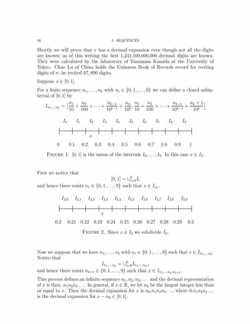
Suppose x ∈ [0, 1].

For a finite sequence n1, . . . , nk with ni ∈ {0, 1, . . . , 9} we can define a closed subin-terval of [0, 1] by

In1,...,nk=

[n1

10+

n2

100+ · · · + nk−1

10k−1+

nk

10k,n1

10+

n2

100+ · · · + nk−1

10k−1+nk + 1

10k

]

0 0.1 0.2 0.3 0.4 0.5 0.6 0.7 0.8 0.9 1

I0 I1 I2 I3 I4 I5 I6 I7 I8 I9

x

Figure 1. [0, 1] is the union of the intervals I0, . . . , I9. In this case x ∈ I2.

First we notice that[0, 1] = ∪9

i=0Ii

and hence there exists n1 ∈ {0, 1, . . . , 9} such that x ∈ In1.

0.2 0.21 0.22 0.23 0.24 0.25 0.26 0.27 0.28 0.29 0.3

I2,0 I2,1 I2,2 I2,3 I2,4 I2,5 I2,6 I2,7 I2,8 I2,9

x

Figure 2. Since x ∈ I2 we subdivide I2.

Now we suppose that we have n1, . . . , nk with ni ∈ {0, 1, . . . , 9} such that x ∈ In1,...,nk.

Notice thatIn1,...,nk

= ∪9i=0In1,...,nk,i

and hence there exists nk+1 ∈ {0, 1, . . . , 9} such that x ∈ In1,...,nk,nk+1.

This process defines an infinite sequence n1, n2, n3, . . . and the decimal representationof x is then .n1n2n3 . . .. In general, if x ∈ R, we let n0 be the largest integer less thanor equal to x. Then the decimal expansion for x is n0.n1n2n3 . . ., where 0.n1n2n3 . . .is the decimal expansion for x− n0 ∈ [0, 1].

7. DECIMALS 27

3.43.

(1) For each k ∈ N define xk ∈ Q by

xk = n0.n1 . . . nk.

Prove that limk→∞

xk = x.

(2) Explain how a real number x may have two decimal expansions.(3) Suppose x, y ∈ R and suppose (ak) and (bk) are decimal expansions for x and

y respectively. In addition, assume neither (ak) nor (bk) ends with a constantsequence of 9’s (see the previous question). Show that x < y if and only ifthere exists a k ∈ N with a0.a1a2 . . . ak < b0.b1b2 . . . bk.

(4) Suppose x, y ∈ R and suppose {ak} and {bk} are decimal expansions for xand y respectively. Describe (and prove) how to find a decimal expansion forx+ y.

(5) Prove that a decimal expansion is eventually periodic if and only if it comesfrom a rational number.

3.44. Let (dn)∞n=1 be an arbitrary sequence with dn ∈ {0, 1, . . . , 9} for each n ∈ N.Define a sequence (an)∞n=1 by

an = 0.d1d2 . . . dn =n∑

k=1

dk

10k.

Prove that (an)∞n=1 converges to a real number. Hence, give another proof that forany a, b ∈ R with a < b there exists a rational number x ∈ (a, b).

CHAPTER 4

Limits and Continuity

1. Limits

The intuitive idea of a number L ∈ R being the limit of a function f(x) as x approachesa point p is that, for all x close enough to p, the value of the function is as close as welike to L. The limit should not depend on the value of f at p but only on the valueof f at points x near p. Indeed for a limit to exist at p it is not even necessary thatf be defined at p but only that f be defined at points x near p.

Definition. Let I ⊆ R be an interval, f : I → R a function, p ∈ I, and L ∈ R. Wesay that L is a limit of f as x approaches p if, for every ε > 0, there exists a δ > 0such that for all x ∈ I if 0 < |x− p| < δ then |f(x) − L| < ε.

When proving that L is a limit of f as x approaches p, we are given an arbitraryε > 0 and have to find a δ > 0 exactly as we had to find a N ∈ N when provingthat L was the limit of a sequence. In practice this means that we seek to estimate|f(x) − L| from above making it < ε using |x− p| < δ.

This definition gives you no way of finding a limit L.

Exactly as for sequences, Problem 3.2, we have to show that limits are in fact unique.

4.1. Let I ⊆ R be an interval, f : I → R a function, and p ∈ I. Suppose L and Mare both limits of f as x approaches p. Show that L = M .

This shows that if a limit of f as x approaches p exists then it is unique. Now we cantalk about the limit of f as x approaches p and write lim

x→pf(x) = L.

Note: When we write limx→p

f(x) = L we are making two assertions; the limit of f as x

approaches p exists, and its value is L. Exactly as with sequences we must take carenever to write lim

x→pf(x) until after we have shown that the limit exists.

If the point p can be approached from both sides by points of I, that is if p ∈ I◦, thenwe can define the left-hand limit and right-hand limit of f as x approaches p.

Definition. Let I ⊆ R be an interval, f : I → R a function, p ∈ I, and L ∈ R. Wesay that L is a right-hand limit of f as x approaches p if for every ε > 0, thereexists a δ > 0 such that I ∩ (p, p + δ) = ∅, and for all x ∈ I if p < x < p + δ then|f(x) − L| < ε. We say that L is a left-hand limit of f as x approaches p if for

29

30 4. LIMITS AND CONTINUITY

p p+ δp− δa b

L

L+ ε

L− ε

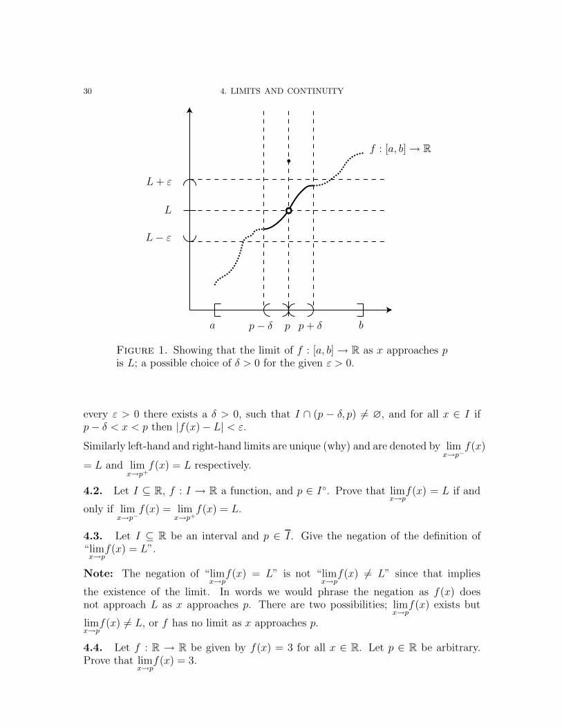
f : [a, b] → R

Figure 1. Showing that the limit of f : [a, b] → R as x approaches pis L; a possible choice of δ > 0 for the given ε > 0.

every ε > 0 there exists a δ > 0, such that I ∩ (p − δ, p) = ∅, and for all x ∈ I ifp− δ < x < p then |f(x) − L| < ε.

Similarly left-hand and right-hand limits are unique (why) and are denoted by limx→p−

f(x)

= L and limx→p+

f(x) = L respectively.

4.2. Let I ⊆ R, f : I → R a function, and p ∈ I◦. Prove that limx→p

f(x) = L if and

only if limx→p−

f(x) = limx→p+

f(x) = L.

4.3. Let I ⊆ R be an interval and p ∈ I. Give the negation of the definition of“lim

x→pf(x) = L”.

Note: The negation of “limx→p

f(x) = L” is not “limx→p

f(x) = L” since that implies

the existence of the limit. In words we would phrase the negation as f(x) doesnot approach L as x approaches p. There are two possibilities; lim

x→pf(x) exists but

limx→p

f(x) = L, or f has no limit as x approaches p.

4.4. Let f : R → R be given by f(x) = 3 for all x ∈ R. Let p ∈ R be arbitrary.Prove that lim

x→pf(x) = 3.

1. LIMITS 31

Remark. In this case the δ that you get does not depend on ε for any p. For afunction f defined on an interval this only occurs when f is constant.

4.5. Let f : R → R be given by f(x) = x for all x ∈ R. Let p ∈ R. Provelimx→p

f(x) = p.

Remark. Now we see that δ depends on ε and that δ goes to 0 as ε goes to 0.However the choice of δ still does not depend on the choice of p.

4.6. Let f : R → R be given by f(x) = 3x − 5 for all x ∈ R. Let p ∈ R. Provelimx→p

f(x) = 3p− 5.

4.7. Let f : R → R be given by f(x) = x2 for all x ∈ R. Let p ∈ R. Provelimx→p

f(x) = p2.

Hint: Start the proof by writing down what needs to be shown. The goal is alwaysto estimate |f(x) − p2| from above by some function of δ that goes to 0 as δ goes to0. By the difference of squares formula, |x2 − p2| = |x + p| |x − p|. The definitionof the limit gives us the estimate |x − p| < δ. However, since our choice of δ is onlyallowed to depend on ε and p but not on x we must estimate |x+p| by some quantityindependent of x.

Since we know that |x− p| < δ we can say |x| < |p| + δ and hence we can estimate

|x+ p| ≤ |x| + |p| < 2|p| + δ

and hence

|x2 − p2| < (2|p| + δ)δ.

Now if we fix an ε > 0 then we can always choose δ > 0 such that (2|p| + δ)δ < ε.If we complete the square or use the quadratic formula then we find an “optimal”choice for δ. However, it is important to remember that we don’t need to find thebest δ we just need to find a δ > 0 that works. If we knew δ ≤ 1 then we couldestimate |x+ p| < 2|p| + 1 and hence |x2 − p2| < (2|p| + 1)δ. From this it is easy tochoose a δ > 0 such that both δ ≤ 1 and (2|p| + 1)δ < ε.

Note: Regardless of how we produce our choice of δ it depends on the point p. Fora fixed ε we see that the δ required gets smaller and smaller as |p| gets bigger andbigger. How could you tell this from looking at the graph of f?

4.8. Using the definition of the limit of a function (i.e., the ε-δ definition), provethat lim

x→2(2x2 − x+ 1) = 7.

4.9. Let I ⊂ R be an interval and let f : I → R, with p ∈ I. Assume there exista < b and δ > 0 such that for all x ∈ I, if |x− p| < δ then f(x) ∈ [a, b]. Prove that ifL = lim

x→pf(x) exists, then L ∈ [a, b].


4.10. Let f : R → R be given by

f(x) =

{0 x is irrational

1 x is rational.

Prove that limx→p

f(x) does not exist for any p ∈ R.


f(x) =

{0 x is irrational

x x is rational.

Prove that limx→p

f(x) exists for only one value of p.

4.12. Let f : [a, b] → R and let p ∈ [a, b]. Assume limx→p

= L exists with L > 0. Prove

that there exists δ > 0 such that if x ∈ [a, b] and 0 < |x− p| < δ then f(x) > L/2.

The next problem relates the limit of a function as x approaches p to the limits ofsequences.

4.13. Let I ⊆ R be an interval, f : I → R a function, p ∈ I, and L ∈ R. Provethat lim

x→pf(x) = L if and only if for every sequence (xn) ⊆ I \ {p} with lim

n→∞xn = p,

we have limn→∞

f(xn) = L.

Hint: To prove “if for every sequence (xn) ⊂ I \ {a} with limn→∞

xn = p we have

limn→∞

f(xn) = L” you should switch to the contrapositive.

4.14. State the contrapositive of the sequential characterization, Problem 4.13, oflimits (i.e., get a new if and only if statement by negating both sides).

This statement is quite useful for proving that a function has no limit as x approachesp.

4.15. Which of these limits (if any) exist? Prove your answer.

(1) limx→0

sin(

1x

).

(2) limx→0

x sin(

1x

).

The following are the analogues of the limit laws for sequences, Problem 3.13.

4.16. Let I ⊆ R be an interval, p ∈ I, and f : I → R and g : I → R functionssatisfying

limx→p

f(x) = L limx→p

g(x) = M

Let c ∈ R. Prove that

(1) limx→p

c · f(x) = c · L.

2. CONTINUOUS FUNCTIONS 33

(2) limx→p

(f(x) + g(x)

)= L+M .

(3) limx→p

f(x) · g(x) = L ·M .

(4) If g(x) = 0 for x ∈ I and M = 0 then limx→p

f(x)g(x)

= LM

.

There are two ways to prove these statements; one is to use the definition of limitdirectly, and the other is to use the sequential characterization of the limit, Problem4.13, and our earlier limit theorems for sequences, Problem 3.13.

Remark. The condition g(x) = 0 for x ∈ I is stronger than necessary. It ensures

that the function f(x)g(x)

is defined for all x ∈ I. If limx→p

g(x) = 0 then there exists an

interval J ⊆ I with p ∈ J and g(x) = 0 for all x ∈ J .

4.17. Let I ⊂ R be an interval, and let p ∈ I. Let f , g, and h be functions onI \ {p} such that g(x) ≤ f(x) ≤ h(x) for all x ∈ I \ {p}. Prove that if lim

x→pg(x) =

limx→p

h(x) = L ∈ R, then limx→p

f(x) = L. (This is the Squeeze Theorem for functions.)

2. Continuous Functions

Definition. Let I ⊆ R be an interval, f : I → R a function, and p ∈ I. We say thatf is continuous at p if for every ε > 0 there exists a δ > 0 such that if x ∈ I and|x− p| < δ then |f(x) − f(p)| < ε.

If f is continuous at all p ∈ I it is called continuous. If S ⊆ I and f is continuousat all p ∈ S it is called continuous on S.

4.18. Let f : I → R where I is an interval and let p ∈ I. Negate the definition of“f is continuous at p”.


f(x) =

{1 0 ≤ x ≤ 1

0 otherwise.

Find all points p ∈ R at which f is continuous. Justify your answer.


f(x) =

{0 x is irrational

1 x is rational.



f(x) =

{0 x is irrational

x x is rational.



The definition of f being continuous at p is very similar to the definition of the limitof f as x approaches p. The following theorem makes the connection explicit. Thisis probably the definition of continuity that you saw in your Calculus class.

4.22. Let I ⊂ R be an interval and p ∈ I. Prove that f is continuous at p if andonly if lim

x→pf(x) = f(p).

Since we have a sequential characterization of the limit of f as x approaches p,Problem 4.13, we can obviously produce a sequential characterization of continuity.

4.23. Let I ⊆ R be an interval, f : I → R a function, and p ∈ I. Prove that f iscontinuous at p if and only if for every sequence (xn) ⊆ I with lim

n→∞xn = p, we have

limn→∞

f(xn) = f(p).

This is slightly different from a direct application of Problem 4.13 since we have everysequence (xn) ⊆ I rather than every sequence (xn) ⊆ I \ {p}. Is the theorem stilltrue if we replace “ every sequence (xn) ⊆ I” with every sequence (xn) ⊆ I \ {p}?4.24. Give the contrapositive to the sequential characterization of continuity, Prob-lem 4.23.

The limit laws for functions, Problem 4.16, can be reinterpreted in terms of continuousfunctions.

4.25. Let I ⊆ R be an interval, f : I → R and g : I → R functions, and p ∈ I.Assume that f and g are continuous at p. Let c ∈ R. Prove

(1) f + g is continuous at p.(2) c · f is continuous at p.(3) f · g is continuous at p.

(4) If g(x) = 0 for x ∈ I then f(x)g(x)

is continuous at p.

4.26. Prove that every polynomial function is continuous on R.

There is one more operation which we can perform with functions that has no directanalogue for sequences.

4.27. Let I, J ⊆ R be intervals, f : I → R and g : J → R functions with f(I) ⊆ J .Let p ∈ I. Prove that if f is continuous at p and g is continuous at f(p) then g ◦ f iscontinuous at p.

This can be proved either directly from the definition or by repeated application ofProblem 4.23.

One of the most important theorems about continuous functions on intervals is the“Intermediate Value Theorem”.

2. CONTINUOUS FUNCTIONS 35

4.28. If f is a continuous function on [a, b] with a < b and f(a) < y < f(b) orf(a) > y > f(b) then there exists p ∈ (a, b) with f(p) = y.

Hint: Suppose f(a) < y < f(b) and let E = {x ∈ [a, b] : f(x) < y}. Let p = supE.The point p can be written as the limit of a sequence xn ∈ E and as the limit of asequence x′n ∈ [a, b] \ E. Hence prove that f(p) = y.

4.29. Let I ⊆ R be any interval and f : I → R a non-constant continuous function.Prove that f(I) is an interval.

Remark. First prove that it suffices to show that given any two points c, d ∈ f(I)the entire interval between them is contained in f(I).

In general we cannot say any more about the interval f(I).

Definition. We say that a function f : I → R is bounded if the set f(I) is bounded.Thus f is bounded if and only if there exists K ∈ R such that |f(x)| ≤ K for allx ∈ I.

4.30. Give an example of a continuous function f : (0, 1) → R that is not bounded.

Thus the continuous image of a bounded interval may be unbounded.

4.31. Give an example of a continuous function f : (0, 1) → R such that f((0, 1)

)is a closed and bounded interval.

Thus the continuous image of an open interval may be a closed interval.

However, in the special case of a continuous function on a closed and bounded intervalwe can say a lot more.

4.32. Let f be a continuous function on [a, b] with a < b. Show that f is bounded.

Hint: Proceed by contradiction. Suppose that f is not bounded above and constructa sequence (xn)∞n=1 with xn ∈ [a, b] for all n ∈ N such that

limn→∞

f(xn) = +∞

Now apply the sequential characterization of continuity, Problem 4.23, to obtain acontradiction.

4.33. Let f be a continuous function on [a, b] with a < b. Show that there existxm, xM ∈ [a, b] such that f(xm) ≤ f(x) ≤ f(xM) for all x ∈ [a, b]. We say f achievesits maximum and minimum value.

Hint: Construct a sequence (xn)∞n=1 with xn ∈ [a, b] for all n ∈ N such that

limn→∞

f(xn) = sup{f(x) : x ∈ [a, b]}.

Now apply the sequential characterization of continuity, Problem 4.23, to find a pointp ∈ [a, b] with f(p) = sup{f(x) : x ∈ [a, b]}.


4.34. Give an example of f : (0, 1) → R that is bounded, continuous, and hasneither a maximum nor a minimum. Can you do the same for f : (0, 1] → R?

3. Uniform Continuity

Sometimes we encounter a property stronger than continuity. Recall that f : I → R

is continuous on I, if for all p ∈ I and for all ε > 0, there exists a δ > 0 such that forall x ∈ I if |x− p| < δ then |f(x) − f(p)| < ε.

For a continuous function, the δ generally depends upon both ε and the point p asprevious exercises have illustrated. If we remove the dependence on p we have uniformcontinuity.

Definition. Let I ⊆ R be an interval and f : I → R a function. We say that f isuniformly continuous on I if for all ε > 0, there exists a δ > 0 such that for allx, y ∈ I if |x− y| < δ then |f(x) − f(y)| < ε.

4.35. Suppose I ⊆ R is an interval. Prove that if f : I → R is uniformly continuouson I then f is continuous on I.

4.36. Let f(x) = mx+c for some m, c ∈ R. Prove that f(x) is uniformly continuouson R.

4.37. Negate the definition of uniform continuity.

4.38. Let f : R → R be given by f(x) = x2. Prove that f is not uniformlycontinuous on R.

Hint: Fix an ε > 0 and show that no matter what δ > 0 is chosen you can alwayschoose x, y ∈ R such that |x− y| < δ and |x2 − y2| ≥ ε.

4.39. Prove that if I is a bounded interval and f : I → R is uniformly continuousthen f is bounded.

This together with Problem 4.30 shows that we can have continuous functions on (0, 1)that are not uniformly continuous. As in the previous section the case of functionson closed and bounded intervals is very different.

4.40. Let f : [a, b] → R be a continuous function. Prove that f is uniformlycontinuous.

Hint: Suppose that f is not uniformly continuous. Then there exists an ε > 0 suchthat for every δ > 0 there exists x, y ∈ [a, b] such that |x−y| < δ but |f(x)−f(y)| ≥ ε.Show that there exists two sequences (xn), (yn) ⊂ [a, b] which both converge to thesame point p ∈ [a, b] but such that |f(xn)− f(yn)| ≥ ε. Hence conclude that f is notcontinuous at p.

CHAPTER 5

Differentiation

1. Derivatives

Definition. Let I ⊂ R be an interval, f : I → R be a function, and p ∈ I0. Thefunction f is said to be differentiable at p if

limx→p

f(x) − f(p)

x− pexists.

If f is differentiable at p then we define the derivative of f at p, denoted f ′(p), by

f ′(p) := limx→p

f(x) − f(p)

x− p

If S ⊆ I, f is said to be differentiable on S if f is differentiable at x for all x ∈ S.

5.1.

(1) Let c ∈ R be arbitrary and f : R → R be defined by f(x) = c. Prove that fis differentiable on R and that f ′(x) = 0 for all x ∈ R.

(2) Let f : R → R be defined by f(x) = x. Prove that f is differentiable on R

and that f ′(x) = 1, for all x ∈ R.(3) Let f : R → R be defined by f(x) = x2−x+1. Prove that f is differentiable

on R and find f ′(x) for x ∈ R.(4) Let f : R → R be defined by f(x) = |x|. Prove that f is not differentiable

at 0.

We can relate the notion of f being differentiable at p with our earlier notion ofcontinuity.

5.2. Let I ⊆ R be an interval, f : I → R a function, and p ∈ I. Prove that f isdifferentiable at p if and only if there exists a function φ : I → R that is continuousat p such that

f(x) = f(p) + (x− p)φ(x).

Moreover, if there exists a function φ : I → R that is continuous at p such that

f(x) = f(p) + (x− p)φ(x),

then f ′(p) = φ(p).

Hint: This is really just a very useful restatement of the definition.

37

38 5. DIFFERENTIATION

Now many of our results about differentiability of f will follow from our rules forcontinuous functions, Problem 4.25, applied to φ.

5.3. Let I ⊆ R be an interval, f : I → R a function, and p ∈ I. Prove that if f isdifferentiable at p then f is continuous at p.

In particular, using Problem 5.2, the usual rules of differentiation come from Problem4.25 by some simple algebra.

5.4. Let I ⊆ R be an interval, f : I → R a function, g : I → R a function, c ∈ R,and p ∈ I. If f is differentiable at p and g is differentiable at p then

(1) c · f is differentiable at p and

(c · f)′(p) = c · f ′(p).

(2) f + g is differentiable at p and

(f + g)′(p) = f ′(p) + g′(p).

(3) f · g is differentiable at p and

(f · g)′(p) = f(p) · g′(p) + f ′(p) · g(p).(4) if g(p) = 0 then f

gis differentiable at p and(fg

)′(p) =

g(p) · f ′(p) − f(p) · g′(p)(g(p)

)2 .

Hint: You can prove these either directly from the definition or by writing f(x) =f(p) + (x − p) · φ(x) and g(x) = g(p) + (x − p) · ψ(x) and using Problem 5.2. Youshould try both ways.

5.5. Let P (x) = a0 + a1x+ · · · + anxn be a polynomial. Prove that for all x

P ′(x) = a1 + 2a2x+ · · · + nanxn−1 .

There is one more standard differentiation rule: the Chain Rule.

5.6. Let I, J ⊆ R be intervals, f : I → R and g : J → R functions with f(I) ⊆ J .Let p ∈ I. Prove that if f is differentiable at p and g is differentiable at f(p) theng ◦ f is differentiable at p and

(g ◦ f)′(p) = g′(f(p)

) · f ′(p).

Hint: Since g is differentiable at f(p) there exists a function ψ : J → R such that

g(x) = g(f(p)

)+

(x− f(p)

) · ψ(x)

for all x ∈ J . Replace x by f(x) and then use the fact that f(x)−f(p) = (x−p)·φ(x).

Perhaps the most important applications of differentiation are in optimization andin estimation. In optimization we try to find the maximum or minimum value of agiven function (often subject to one, or more, constraints).

2. THE MEAN VALUE THEOREM 39

2. The Mean Value Theorem

Definition. Let I ⊆ R be an interval and f : I → R a function. We say p ∈ I isa local maximum if there exists a δ > 0 such that for all x ∈ I with |x − p| < δ,f(x) ≤ f(p). We say p ∈ I is a local minimum if there exists a δ > 0 such that forall x ∈ I with |x− p| < δ, f(x) ≥ f(p).

We begin with a lemma that relates local maxima and minima with differentiation.

5.7. Let I ⊆ R be an interval and f : I → R a function. Prove that if p ∈ I◦ is eithera local maximum or a local minimum, and f is differentiable at p, then f ′(p) = 0.

Hint: Assume p is a local maximum and compute the signs of

limx→p+

f(x) − f(p)

x− pand lim

x→p−

f(x) − f(p)

x− p.

If f is differentiable at p then these limits must be equal.

With this observation we can prove Rolle’s Theorem. A version of the theorem wasfirst stated by Indian astronomer Bhaskara in the 12th century however the first proofseems to be due to Michel Rolle in 1691.

5.8. Let a < b. Prove that if f : [a, b] → R is continuous, f is differentiable on(a, b), and f(a) = f(b), then there exists a point p ∈ (a, b) with f ′(p) = 0.

Hint: If f is not constant it has either a maximum value or a minimum value atsome c ∈ (a, b).

An immediate consequence of Rolle’s Theorem is the very important Mean ValueTheorem. The Mean Value Theorem is used extensively in estimation.

5.9. Let a < b. Prove that if f : [a, b] → R is continuous and f is differentiable on(a, b) then there exists c ∈ (a, b) with

f ′(c) =f(b) − f(a)

b− a.

Hint: Construct a linear function l(x) with l(a) = f(a), l(b) = f(b) and considerg(x) = f(x) − l(x).

We now give some consequences of the Mean Value Theorem.

5.10. Let a < b. Prove that if f : [a, b] → R is continuous, f is differentiable on(a, b), and f ′(p) = 0 for all p ∈ (a, b) then f(x) is a constant.

5.11. Let a < b, f : [a, b] → R be continuous, and f differentiable on (a, b). Provethat

(1) if f ′(x) ≥ 0 for all x ∈ (a, b) then f is increasing on [a, b], i.e. if a ≤ x < y ≤ b,then f(x) ≤ f(y).

40 5. DIFFERENTIATION

(2) if f ′(x) ≤ 0 for all x ∈ (a, b) then f is decreasing on [a, b], i.e. if a ≤ x < y ≤b, then f(x) ≥ f(y).

CHAPTER 6

Integration

1. The Definition

Our final chapter is the other half of calculus, the definite integral. Again let’s recalla familiar problem to motivate our definition.

Problem. Let f : [a, b] → [0,∞) be continuous. Find the area of the region boundedby x = a, x = b, y = f(x) and y = 0. Draw a few pictures of such f ’s, e.g., f(x) = x2

on [0, 2]. Geometry does not give us a formula for this area unless f is quite nice(e.g., f(x) = 3). Our approach for finding this area will be to use very thin rectanglesto approximate the area and then use a limiting process to obtain the area. It lookscomplicated so be sure to draw some pictures to help you understand the notation.

In this chapter we define∫ b

af(x) dx, commonly called the (definite) Riemann in-

tegral of f over [a, b]. You should recall from calculus the “short way” of computingthis: ∫ 2

1

x dx =x2

2

∣∣∣21

= 2 − 1

2=

3

2.

This comes from the fundamental theorem of calculus, which we shall prove. We will

define∫ b

af(x) dx so that when f ≥ 0 and f is continuous, this number is the area of

the region bounded by y = f(x), x = a, x = b and the x-axis.

Definition. Let a < b. Let f : [a, b] → R be a bounded function.

A partition P of [a, b] is an ordered finite set

a = x0 < x1 < · · · < xn = b.

If P and Q are two partitions of [a, b] we say that Q refines P if Q ⊇ P .

Let P = (x0, x1, . . . , xn) be a partition of [a, b]. For 1 ≤ i ≤ n we set

Mi(f, P ) = sup{f(x) : xi−1 ≤ x ≤ xi}= sup f

([xi−1, xi]

)mi(f, P ) = inf{f(x) : xi−1 ≤ x ≤ xi}

= inf f([xi−1, xi]

)Δi = xi − xi−1.

41

42 6. INTEGRATION

We define the upper Riemann sum of f with respect to P , denoted U(f, P ), by

U(f, P ) =n∑

i=1

Mi(f, P ) Δi

and we define the lower Riemann sum of f with respect to P , denoted L(f, P ), by

L(f, P ) =

n∑i=1

mi(f, P ) Δi.

6.1. Let f(x) = x and g(x) = x2 for x ∈ [0, 1]. Let n ∈ N and let Pn ={0, 1

n, 2

n, · · · , n−1

n, 1} be a partition of [0, 1]. Draw a picture illustrating L(f, P4),

U(f, P4), L(g, P4), and U(g, P4). Can you find expressions for L(f, Pn), U(f, Pn),L(g, Pn), and U(g, Pn)?

6.2. Let f : [a, b] → R be bounded and let P be a partition of [a, b]. Let m =inf f([a, b]) and M = sup f([a, b]).

(1) Provem (b− a) ≤ L(f, P ) ≤ U(f, P ) ≤M (b− a).

(2) Prove that if Q refines P then

L(f, P ) ≤ L(f,Q) ≤ U(f,Q) ≤ U(f, P ).

Hint: First prove that it suffices to show this when |Q| = |P | + 1. Thenprove (2) in this case.

Definition. Let f : [a, b] → R be bounded. We define the upper Riemann integralof f , denoted U(f), by

U(f) = inf{U(f, P ) : P is a partition of [a, b]

}.

We define the lower Riemann integral of f , denoted L(f), by

L(f) = sup{L(f, P ) : P is a partition of [a, b]

}.

(Why do these exist?) We say f is Riemann integrable if L(f) = U(f). In this casewe call the common value the (definite) Riemann integral of f over the interval

[a, b] which we denote∫ b

af . Remember that the infimum or supremum of a set may

not be a member of that set.

6.3. Show that for f and g as in Problem 6.1 for all n ∈ N, U(f, Pn) = U(f),L(f, Pn) = L(f) and similarly for g.

We begin by seeing that not every bounded function is integrable. Later we will provethat every continuous function is integrable.

6.4. Let f : [0, 1] → R be given by

f(x) =

{0 x ∈ [0, 1] \ Q

1 x ∈ [0, 1] ∩ Q.

2. INTEGRABLE FUNCTIONS 43

Prove, or disprove, the statement: f is integrable.

6.5. Let f : [a, b] → R be bounded and let P and Q be partitions of [a, b]. Provethat L(f, P ) ≤ U(f,Q).

Hint: Consider the partition R = P ∪Q.

6.6. Let f : [a, b] → R be bounded. Show that L(f) ≤ U(f).

6.7. Let f : [0, 1] → R be given by f(x) = x for all x ∈ [0, 1]. Let Pn be the partitionof [0, 1] given by

Pn = (0,1

n,2

n, . . . ,

n− 1

n, 1).

(1) Find L(f, Pn) and U(f, Pn).(2) Find U(f, Pn) − L(f, Pn).

(3) Show f is integrable on [0, 1] and find∫ 1

0f .

Remark. Notice for any partitions P , Q, we have U(f, P ) = L(f,Q), even thoughU(f) = L(f).

2. Integrable Functions

The definition of integrability can be difficult to use directly so we are fortunate tohave this next problem.

6.8. Let f : [a, b] → R be bounded. Show that f is integrable on [a, b] if and only iffor all ε > 0 there exists a partition P = (x0, . . . , xn) of the interval [a, b] such that

U(f, P ) − L(f, P ) =

n∑i=1

(Mi(f, P ) −mi(f, P )

)Δi < ε.

6.9. Let f : [a, b] → R be an increasing function. Prove that f is integrable on [a, b].

Hint: For an increasing function we know explicitly what Mi(f, P ) and mi(f, P ) are.

6.10. Let f : [a, b] → R be continuous. Prove that f is integrable on [a, b].

Hint: Use Problem 4.40 to conclude that f is uniformly continuous. Let ε > 0 bearbitrary and choose δ > 0 so that if x, y ∈ [a, b] with |x−y| < δ then |f(x)−f(y)| <

εb−a

. Let P be any partition with each Δix < δ and use Problem 6.8.

6.11. Let f and g be integrable functions on [a, b]. Let c ∈ R be an arbitrary constant.Prove that

(1) c · f is integrable on [a, b] and∫ b

a

c · f = c

∫ b

a

f.

44 6. INTEGRATION

(2) f + g is integrable on [a, b] and∫ b

a

(f + g) =

∫ b

a

f +

∫ b

a

g.

Hint: Show

Mi(f + g, P ) ≤Mi(f, P ) +Mi(g, P )

and hence conclude that U(f + g, P ) ≤ U(f, P ) + U(g, P ). Similarly, show thatL(f + g, P ) ≥ L(f, P ) + L(g, P ). Use Problem 6.8 to conclude integrability. Thenprove the equation.

Look at f(x) = x and g(x) = 1− x on the interval I = (0, 1). Then sup(f(I)) = 1 =sup(g(I)) and inf(f(I)) = 0 = inf(g(I)) (notice that neither f nor g has a maximumor a minimum on I). The function (f + g)(x) = f(x) + g(x) = x+ 1 − x = 1, and istherefore constant on I. Thus, sup((f + g)(I)) = 1 < 1 + 1 = sup(f(I)) + sup(g(I))and inf((f + g)(I)) = 1 > 0 + 0 = inf(f(I)) + inf(g(I)).

6.12. Let f and g be integrable on [a, b] with f(x) ≤ g(x) for all x ∈ [a, b]. Prove

that∫ b

af ≤ ∫ b

ag.

6.13. Let a < c < b and let f : [a, b] → R.

(1) Assume f is integrable on [a, b]. Prove that f is integrable on [a, c] and [c, b].(2) Assume that f is integrable on [a, c] and on [c, b]. Prove that f is integrable

on [a, b] and ∫ b

a

f =

∫ c

a

f +

∫ b

c

f .

Definition. If f is integrable on [a, b] we define∫ a

bf = − ∫ b

af . We define

∫ a

af = 0.

6.14. Let f be integrable on an interval containing a, b and c. Prove that, no matterwhat their order, ∫ b

a

f =

∫ c

a

f +

∫ b

c

f .

6.15. Let f : [a, b] → R be integrable. Prove that

(1) |f | is integrable on [a, b]Hint: Prove that Mi(|f |, P ) −mi(|f |, P ) ≤ Mi(f, P ) −mi(f, P ).

(2)∣∣∫ b

af∣∣ ≤ ∫ b

a|f |.

6.16. Prove that if f and g are integrable on [a, b] then f · g is integrable on [a, b].

Hint: Since f and g are integrable we may define

Lf = sup{|f(x)| : a ≤ x ≤ b},Lg = sup{|g(x)| : a ≤ x ≤ b}.

3. FUNDAMENTAL THEOREMS OF CALCULUS 45

Use the fact that

f(x) · g(x) − f(y) · g(y) = f(x) · (g(x) − g(y))

+(f(x) − f(y)

) · g(y)to conclude

Mi(f · g, P )−mi(f · g, P )

≤ Lf · (Mi(g, P )−mi(g, P ))

+(Mi(f, P ) −mi(f, P )

) · Lg.

Now use Problem 6.8

3. Fundamental Theorems of Calculus

Finally we reach the Fundamental Theorem of Calculus which relates integration anddifferentiation. It is commonly broken into two different theorems.

6.17. Prove the first Fundamental Theorem of Calculus:

Let f be integrable on [a, b]. Define a function F : [a, b] → R by

F (x) =

∫ x

a

f.

F is uniformly continuous on [a, b], and if f is continuous at c ∈ (a, b) then F ′(c) =f(c).

Hint: For uniform continuity show that if a ≤ x ≤ y ≤ b then

F (y) − F (x) =

∫ y

x

f.

Now estimate∫ y

xf from above and below in terms of y − x. For F ′(c) = f(c) show

thatF (x) − F (c)

x− c− f(c) =

1

x− c

∫ x

c

[f − f(c)] .

Use the fact that f is continuous at c to conclude that the right hand side can bemade arbitrarily small by taking x sufficiently close to c.

6.18. Prove the second Fundamental Theorem of Calculus:

If f is differentiable on [a, b] and f ′ is integrable on [a, b], then∫ b

af ′ = f(b) − f(a).

Hint: If P = (x0, x1, . . . , xn) is any partition of [a, b] then, by Problem 5.9, for each1 ≤ i ≤ n we can find ti ∈ (xi−1, xi) so that

f(b) − f(a) =

n∑i=1

(f(xi) − f(xi−1)

)=

n∑i=1

f ′(ti)Δi .

Show L(f ′, P ) ≤ f(b) − f(a) ≤ U(f ′, P ).

46 6. INTEGRATION

4. Integration Rules

Once we have the fundamental theorems of calculus we can prove two of the importantrules of integration; integration by parts, and integration by substitution. These turnout to be reinterpretations of the product rule from differentiation and the chain rulerespectively.

6.19. Prove that if f and g are functions that are differentiable on [a, b] and bothf ′ and g′ are integrable on [a, b] then∫ b

a

f(x) · g′(x) = f(b) · g(b) − f(a) · g(a) −∫ b

a

f ′(x) · g(x).

Hint: By Problem 5.4 f · g is differentiable and (f · g)′ = f ′ · g + f · g′.6.20. Suppose that u is differentiable on [c, d] and u′ is continuous on [c, d]. Leta = u(c) and b = u(d). Suppose that f is continuous on u

([c, d]

). Prove that∫ b

a

f =

∫ d

c

(f ◦ u) · u′.

Hint: Let F (x) =∫ x

af . Use Problem 6.17 to show that F is differentiable and use

Problem 5.6 to show that F ◦ u is differentiable. Now apply Problem 6.18.

Remark. Notice we don’t need to assume that u([c, d]

)= [a, b].

Appendix to Chapter 2

1. The Field Properties

Mathematicians study many different types of mathematical objects. You may haveheard of groups, rings, topological spaces, smooth manifolds, vector spaces, Banachspaces, affine varieties, elliptic curves, etc. One of the objects which mathematiciansstudy is called a field. In the introduction to the chapter, we mentioned severalalgebraic properties of R. The crucial algebraic properties of R can be summarizedby saying that R is a field. Notice that all the field properties (listed below) wouldcertainly be demanded of any number system.

As we mentioned above, we will take all the properties on faith. Hence will call themaxioms (in mathematics an axiom is a basic statement which is accepted withoutproof, for example the statement which says “There exists a set” is a basic axiom ofmathematics).

Axiom 1. There exists a set R, which contains Q. We may define two operations on R

called addition and multiplication, which extend normal addition and multiplicationof rational numbers.

When we say that addition on R extends addition on Q, we mean that adding tworeal numbers which happen to be rational would be the same as the normal additionof rational numbers (and likewise for multiplication).

We will use all the standard notations regarding operations among numbers. Forexample a + b is the sum of a, b ∈ R. As always, we write the symbol ‘=’ betweentwo real numbers which are the same and the symbol ‘=’ between two which are not.

Axiom 2. Addition of real numbers is commutative: For every a, b ∈ R, a+b = b+a.

Axiom 3. Addition of real numbers is associative: For every a, b, c ∈ R, a+(b+ c) =(a+ b) + c.

Axiom 4. The real number zero is an additive identity: For each a ∈ R, 0 + a = a.

Axiom 5. Every real number has an additive inverse: For every a ∈ R, there is anumber b ∈ R such that a+ b = 0.

We mentioned above that there are many obvious facts about the real numbers that,strictly speaking, must be proven from the axioms. The following is an example (asare most of the exercises in this section).

47

48 APPENDIX TO CHAPTER 2

A2.1. For every a ∈ R, the additive inverse of a is unique. That is, if b and c arereal numbers which satisfy a + b = 0 and a + c = 0, we may conclude that b = c.

The previous problem justifies us saying THE additive inverse of a ∈ R (rather thenAN additive inverse). As usual, we will use the symbol −a for the additive inverse ofa. Notice that, strictly speaking, −a is not the same symbol as (−1) · a (that is thenumber negative 1 times the number a). That the two symbols represent the samenumber will be one the obvious facts we prove below.

We can also now define subtraction: If a and b are natural numbers, then a − b isdefined to be a+ (−b) (in words a− b is the the sum of a and the additive inverse ofb).

Axiom 6. Multiplication of real numbers is commutative: For every a, b ∈ R, ab = ba.

Axiom 7. Multiplication of real numbers is associative: For every a, b, c ∈ R, a(bc) =(ab)c.

Axiom 8. The number one is a multiplicative identity: For every a ∈ R, a · 1 = a.

Axiom 9. Every real number besides zero has a multiplicative inverse: For everya ∈ R, a = 0, there is a number b such that ab = 1.

We have a result about multiplicative inverses analogous to the one we had for additiveinverse.

A2.2. For every a ∈ R (other than zero), the multiplicative inverse of a is unique.That is, if b and c are real numbers which satisfy ab = 1 and ac = 1, we may concludethat b = c.

Again we are now justified in referring to THE multiplicative inverse of a, whichwe will denote by a−1. We define division in a similar manner as subtraction: a/b isdefined to be ab−1 (that is, a/b is defined to be the product of a and the multiplicativeinverse of b).

Axiom 10. Multiplication and addition satisfy the distributive property: For everya, b, c ∈ R, a(b+ c) = ab+ ac.

These algebraic properties of the real numbers are very important, but they are notunique to R. Q would satisfy all of these axioms and so is also a field. In general,there exist many different fields. The collection of complex numbers, C, (with usualnotions of addition and subtraction) is a field. For a prime number p, you may befamiliar with the collection of numbers modulo p, often denoted Zp. It too is a field(and in contrast to Q, R, and C has finitely many elements). We will thus need moreproperties of R to describe it uniquely.

The following (relatively simple) question might help you to better understand theaxioms:

2. THE ORDER PROPERTIES 49

A2.3. Which axioms would still be satisfied if R were replaced with Q? with Z?with N?

We will now give some more basic properties about the real numbers which followfrom these axioms.

For our first result, we will see that the multiplication operation on R still boils downto repeated addition (as long as one of the numbers is a natural number).

A2.4. Multiplication of real numbers by natural numbers is just repeated addition.That is, if a ∈ R, and n ∈ N, na is the same as the number which results when a isadded to itself n times.

Hint: Use induction.

As promised, we will show that the additive inverse of a real number is just thatnumber, multiplied by −1.

A2.5. For every a ∈ R, the product of a and −1 is the additive inverse of a. Thatis, −a = (−1)a.

We can also define integral powers of real numbers in the usual way.

Definition. Let a ∈ R. If n is a natural number, we define an to be the product ofa with itself n times. If a−n is defined to be the product of a−1 with itself n times.We also define a0 to be 1.

We have the following basic properties of powers:

A2.6. If a, b ∈ R and m,n ∈ Z, then

(1) (am)n = amn = (an)m,(2) am+n = aman, and(3) (ab)m = ambm.

Hint: These properties are by no means automatic. They must be proven, bycareful reasoning, from the axioms.

2. The Order Properties

In the previous section we saw the algebraic (or field) properties of R. In this one wewill study the order properties. As mentioned in the introduction, a set is ordered ifwe have a rule which tells us, given two elements of the set, which is bigger.

Axiom 11. The real numbers come equipped with an order which extends the orderon Q.

By ‘extends,’ we mean that if a and b are rational numbers, then a is less than baccording to the order on Q if and only if a is less than b according to the order onR.


As usual, we denote the order by ≤.

Axiom 12. The order is reflexive: For every a ∈ R, a ≤ a.

Axiom 13. The order is transitive: For every a, b, c ∈ R such that a ≤ b and b ≤ c,we have a ≤ c.

Axiom 14. The order is antisymmetric: For every a, b ∈ R such that a ≤ b and b ≤ a,we have a = b.

Axiom 15. The order is a total order: For every a, b ∈ R, either a ≤ b or b ≤ a.

R is by no means the only set that comes with an order. In fact, an order can bedefined on any set (and many sets, like for example the set consisting of all the monthsin the year, have an obvious order). Actually, there are many different ways to definean order on R, but there is only one order that will satisfy all the axioms we will list(and have listed).

We will also use the symbols <, >, and ≥ with their usual meanings (i.e., a < bmeans a ≤ b and a = b). To make our words precise, we will pronounce a ≤ b as “ais less than b” and a < b as “a is strictly less than b” (with similar phrasing for ≥and >). Note then that “a is less than b” includes the possibility that a = b. This isonly a convention, but it is one used by many mathematicians.

Again we have many basic and obvious properties.

A2.7. R satisfies the trichotomy property: if a, b ∈ R, then exactly one of thefollowing holds:

(1) a < b,(2) a > b, or(3) a = b.

As expected, a number which is strictly greater than zero is called positive, whereasa number which is either positive or zero (in other words a number that is greaterthen zero) is called nonnegative. We use the terms negative and nonpositivesimilarly (though nonpositive is typically used with less frequency).

3. The Ordered Field Properties

In this section, we will discuss how the algebraic (field) properties of R interact withthe order properties (again in ways that, if you think about them, should work in anysystem of numbers).

Axiom 16. The order is preserved under addition by a fixed number: If a, b, c ∈ R

and a ≤ b then a+ c ≤ b+ c.

Axiom 17. The product of two nonnegative numbers is again nonnegative: If a, b ∈ R,0 ≤ a, and 0 ≤ b then 0 ≤ ab.

3. THE ORDERED FIELD PROPERTIES 51

To say that R satisfies these additional properties is to say that it is an ordered field.Notice that being an ordered field is much more restrictive than being a field andhaving an order. The field properties and the order properties must also interactin the right way (as described by the previous two axioms). For example, althoughthere many orders on the set of complex numbers, C, there is no order which makesit into an ordered field (this is not too difficult to prove and we will do so below).Demanding that our numbers form an ordered field tells us that we cannot includeimaginary numbers (or complex numbers) in our number system. It also turns outthat there is no order on Zp which makes it into an ordered field.

Nevertheless, R is not the only ordered field. Q is an ordered field and there aremany others. We will need one additional property, called the completeness axiom,to uniquely define R. As we mentioned above, the completeness axiom is significantlydeeper than the others and we will need to develop several new concepts in the nextchapter before we can describe it.

Again we have many basic properties that follow from the axioms. As always, becareful not to use any facts other than the axioms (and other facts we have proven).

The next result shows that we may multiply inequalities by −1 as long as we arewilling to reverse the sign.

A2.8. Let a, b ∈ R. If a ≤ b then −b ≤ −a.More generally we may multiply an inequality by a real number, but, as expected, wemust reverse the sign if the number is negative.

A2.9. Suppose a, b ∈ R and a ≤ b. If c ∈ R is nonnegative, then ac ≤ bc. If c isnonpositive then bc ≤ ac.

Of course the same result holds for strict inequalities unless c = 0 (by a similar proof).

A2.10. Given any number a ∈ R, there is a number which is strictly larger.

Hint: Finding a number is not difficult, but prove rigorously that it is larger.

A2.11. If a ∈ R, a2 ≥ 0 with a2 = 0 if and only if a = 0.

We will not have occasion to use the next two results, but they are of general interestand they provide insights into ordered fields.

A2.12. Suppose we have a field F (that is, F satisfies all the properties which wegave for R in the section on the field properties). In addition suppose there is anelement i ∈ F which satisfies i2 = −1. Then there is no order on F which makes itinto an order field (that is, no order which will satisfy all the properties given for R

in this chapter).

Hint: Suppose F does indeed satisfy all the properties we have given so far for R.How does i compare to zero?

A2.13. There is no order on C which makes it an ordered field.


This last result is important because C does satisfy the completeness axiom. Thusthere are fields other then R which satisfy the completeness axiom, but no otherordered fields which satisfy it. Notice that Q is an ordered field which is not completeand C is a completed field which is not ordered.

All of the assumed properties of R are now in place except completeness. The re-maining statements of this chapter must therefore be proven from our axioms.

4. Set Theory

We will not try and define what we mean by a set. Surprisingly this is actually quitecomplicated and there is a branch of mathematical logic called set theory that dealswith this.

Definition. The basic set theory concepts we expect you to be familiar with are:

(1) ∅ is the empty set, i.e. the set with no elements.(2) A ⊆ B means that every element of A is an element of B, or for all x ∈ A,

x ∈ B. It is read “A is a subset of B.”(3) A = B means that A and B have the same elements. Another way of saying

this is x ∈ A if and only if x ∈ B.(4) A ∩ B = {x : x ∈ A and x ∈ B}. A ∩ B is read as “A intersect B” and is

called the intersection of A and B.(5) A ∪ B = {x : x ∈ A or x ∈ B}. A ∪ B is read as “A union B” and is called

the union of A and B. If x ∈ A ∪ B then x ∈ A or x ∈ B. It could be inboth.

(6) A and B are called disjoint sets if A ∩ B = ∅. A and B are disjoint if theyhave no elements in common.

It turns out that the operations of union and intersection satisfy “distributive laws”reminiscent of those that hold for the real numbers:

Theorem A2.14. Suppose that A, B, and C are sets. Then the following identitieshold:

(1) A ∩ (B ∪ C) = (A ∩B) ∪ (A ∩ C)(2) A ∪ (B ∩ C) = (A ∪B) ∩ (A ∪ C)

Definition.

(1) A \B = {x : x ∈ A and x /∈ B}. A \B is read as “A minus B” and is calledthe “set theoretic difference of A and B.”

(2) A�B = (A\B)∪ (B \A) and is called the symmetric difference of A andB.

(3) Ac = {x : x /∈ A} is called the complement of A.

5. CARDINALITY 53

Caution: To be honest Ac is not really a set since we have not said what x is otherthan it is not in A. When we use Ac we must have a universal set U in mind. Theuniversal set is often unspecified and is simply inferred from the context. Then wecan write Ac = U \ A which is unambiguous.

Theorem A2.15. Let A and B be sets. Then the following are true:

(1) (Ac)c = A.(2) (A ∩ B)c = Ac ∪Bc.(3) (A ∪ B)c = Ac ∩Bc.(4) A�B = (A ∪ B) \ (A ∩ B).

Statements (2) and (3) are called De Morgan’s Laws.

Definition. If A and B are sets then the Cartesian product of A and B is definedto be

A×B = {(a, b) : a ∈ A and b ∈ B}where (a, b) denotes the ordered pair.

R2 = R × R is the Cartesian plane.

Definition. We can define unions and intersections of large collections of sets. If Iis a set, called the index set, and for all i ∈ I, Ai is a set then we define⋃

i∈I

Ai = {x : there exists i ∈ I such that x ∈ Ai}⋂i∈I

Ai = {x : for all i ∈ I, x ∈ Ai}.

Theorem A2.16. If I is a set and for all i ∈ I, Ai is a set, then

(1) (⋃i∈I

Ai)c =

⋂i∈I

Aci .

(2) (⋂i∈I

Ai)c =

⋃i∈I

Aci .

These are the De Morgan’s laws for unions and intersections over arbitrary index sets.

5. Cardinality

Having defined “function” we can proceed to some fun stuff concerning counting thenumber of elements in a set. How can you count an infinite set? How can youdetermine if two sets (even infinite ones) have the same number of elements, or as weshall say the same cardinality? Your first notions of size may be shattered. Read on.

Definition. If A and B are sets we write |A| = |B| if there exists a 1–1 onto functionf : A→ B. We read |A| = |B| as “the cardinality of A equals the cardinality of B.Note. By Theorem 2.7 in Chapter 2, |A| = |B| ⇒ |B| = |A|.


Intuitively |A| = |B| means that both sets have the “same number of elements”. Thisis not startling for finite sets. It is no surprise that |{a, b, c}| = |{1, 2, 3}|. Howeverthis definition can lead to non-intuitive results. We can have A ⊆ B, A = B yet|A| = |B| (how?).

Definition. A is finite if A = ∅ or if there exists n ∈ N with |A| = |{1, 2, . . . , n}|.(We then say |A| = 0 or |A| = n accordingly.) A is infinite if A is not finite. A iscountably infinite if |A| = |N|. A is countable if A is finite or countably infinite.

Are all infinite sets also countably infinite?

A2.17. Prove that a set A is

a) countably infinite if and only if we can write A = {a1, a2, . . .} where ai = aj

if i = j.b) countably infinite if and only if A is infinite and we can writeA = {a1, a2, . . .}.c) countable if and only if A = ∅ or we can write A = {a1, a2, . . .}.

Deduce that if B ⊆ A and A is countable, then B is countable.

A2.18. Let |A| = |B| and |B| = |C|. Prove that |A| = |C|.A2.19. Prove that

a) |N| = |{2, 4, 6, 8, . . .}|b) |N| = |Z|c) |N| = |{x ∈ Q : x > 0}|

Hint: Try to make an infinite list of all rationals in (0, 1]. Now try to make a list ofall rationals > 1.

d) |N| = |Q|.A2.20. If A is countable and B is countable prove that A× B is countable.

Hint: You want to construct a list of all elements in A×B (see 1.17). Can you makean infinite matrix of these elements starting with

a1 a2 a3 . . .

b1b2b3...

Can you take this matrix and make a list as in 1.17c)?

Our next problem is due to G. Cantor. It is a famous result which shook the math-ematical world and has found its way into numerous “popular” math/science books.Cantor went insane. The problem’s solution relies on the decimal representation of a

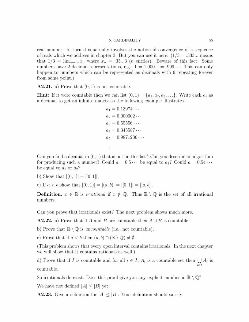
5. CARDINALITY 55

real number. In turn this actually involves the notion of convergence of a sequenceof reals which we address in chapter 3. But you can use it here. (1/3 = .333... meansthat 1/3 = limn→∞ xn where xn = .33...3 (n entries). Beware of this fact: Somenumbers have 2 decimal representations, e.g., 1 = 1.000... = .999... . This can onlyhappen to numbers which can be represented as decimals with 9 repeating foreverfrom some point.)

A2.21. a) Prove that (0, 1) is not countable.

Hint: If it were countable then we can list (0, 1) = {a1, a2, a3, . . .}. Write each ai asa decimal to get an infinite matrix as the following example illustrates.

a1 = 0.13974 · · ·a2 = 0.000002 · · ·a3 = 0.55556 · · ·a4 = 0.345587 · · ·a5 = 0.9871236 · · ·...

Can you find a decimal in (0, 1) that is not on this list? Can you describe an algorithmfor producing such a number? Could a = 0.5 · · · be equal to a1? Could a = 0.54 · · ·be equal to a1 or a2?

b) Show that |(0, 1]| = |[0, 1]|.c) If a < b show that |(0, 1)| = |(a, b)| = |[0, 1]| = |[a, b]|.Definition. x ∈ R is irrational if x /∈ Q. Thus R \ Q is the set of all irrationalnumbers.

Can you prove that irrationals exist? The next problem shows much more.

A2.22. a) Prove that if A and B are countable then A ∪ B is countable.

b) Prove that R \ Q is uncountable (i.e., not countable).

c) Prove that if a < b then (a, b) ∩ (R \ Q) = ∅.(This problem shows that every open interval contains irrationals. In the next chapterwe will show that it contains rationals as well.)

d) Prove that if I is countable and for all i ∈ I, Ai is a countable set then⋃i∈I

Ai is

countable.

So irrationals do exist. Does this proof give you any explicit number in R \ Q?

We have not defined |A| ≤ |B| yet.

A2.23. Give a definition for |A| ≤ |B|. Your definition should satisfy


a) |A| ≤ |A|b) |A| ≤ |B| and |B| ≤ |C| implies that |A| ≤ |C|.

Bonus. Prove also that

c) |A| ≤ |B| and |B| ≤ |A| iplies that |A| = |B|.Definition. |A| < |B| if |A| ≤ |B| and |A| = |B|.

A2.24. Prove that for all sets A, |A| < |P(A)| (so no largest “cardinal number”exists). Hint: Show there does not exist a function f : A → P(A) which is onto byassuming such an f exists and considering B ∈ P(A) where B = {a ∈ A : a /∈ f(a)}.Note: P(A) denotes the set of all subsets of A. Thus P({1, 2}) = {φ, {1}, {2}, {3}}.

6. Mathematical Induction

The Theorem of Mathematical Induction. Let P (1), P (2), P (3), . . . be a listof statements, each of which is either true or false. Suppose that

i) P (1) is trueii) For all n ∈ N, if P (n) is true then P (n+ 1) is true.

Then for all n ∈ N, P (n) is true.

A2.25. Prove this theorem.

Hint: Suppose it were not true. Choose n0 to be the smallest integer so that P (n0)is false.

A2.26. Use mathematical induction to establish the following. Make sure in yourproof to precisely state what you are taking “P (n)” to be.

a) For all n ∈ N, 1 + 2 + · · ·+ n = n(n+1)2

b) For all n ∈ N, 12 + 22 + · · ·+ n2 = n(n+1)(2n+1)6

c) For all n ∈ N, if n ≥ 4 then 2n < n!.

Note: n! = 1 · 2 · 3 · · · · · (n− 1) · n. This is called “n factorial.”

Appendix to Chapter 3

1. Open and Closed Sets

Continuing our discussion of R we turn to what is called “topology”. This is crucialmaterial for our future discussion of limits and continuity.

Definition. Let ε > 0. The interval (a − ε, a + ε) is said to be an open intervalcentered at a of radius ε.

A3.1. Let a < b. Show that (a, b) is an open interval of radius ε for some ε > 0.What is the center? What is ε?

Definitions. Let S ⊆ R.

a) S is open if for all a ∈ S there exists ε > 0 with (a− ε, a+ ε) ⊆ Sb) S is closed if C(S) = R \ S is open.

Quick Question: Is every S ⊆ R either open or closed? Can you justify youranswer?

A3.2. Prove that every open interval is an open set and every closed interval is aclosed set.

A3.3. Classify as open, closed, both or neither

a) ∅ b) [0, 1] c) Q d) R \ Q e) R f) [0, 1] ∪ [2, 3] g) { 1n

: n ∈ N}Definitions. Let S ⊂ R.

a) x ∈ int(S) if there exists ε > 0 with (x− ε, x+ ε) ⊆ S.b) x ∈ bd(S) if for all ε > 0, (x−ε, x+ ε)∩S = ∅ and (x−ε, x+ ε)∩C(S) = ∅.

Note: “int” is short for interior and “bd” is short for boundary .

A3.4. For each S find int(S) and bd(S)

a) [0, 1] b) (0, 1) c) Q d) R e) {1, 2, 3} f) { 1n

: n ∈ N}A3.5. Prove the following. S ⊆ R.

a) int(S) ⊆ S and int(S) is an open set.

57


b) S is open ⇔ S = int(S).c) S is open ⇔ S ∩ bd(S) = ∅.d) S is closed ⇔ S ⊇ bd(S).

A3.6. Prove the following

a) If I is a set and for all i ∈ I, Ai is an open set, then⋃i∈I

Ai is open.

b) If I is any set and for all i ∈ I, Fi is a closed set then⋂i∈I

Fi is closed.

c) If n ∈ N and Ai is an open set for each i ≤ n thenn⋂

i=1

Ai is open.

d) If n ∈ N and Ai is a closed set for each i ≤ n thenn⋃

i=1

Ai is closed.

A3.7. Show by example that c) (and d)) in 2.17 cannot be extended to infiniteintersections (unions).

Definitions. Let S ⊆ R, x ∈ R.

a) x is an accumulation point of S if for all ε > 0, {y ∈ R : 0 < |x − y| <ε} ∩ S = ∅.

b) S ′ = {x : x is an accumulation point of S}.c) x is an isolated point of S if x ∈ S \ S ′.d) S = S ∪ S ′.

Note: S is called the closure of S.

A3.8. Let S ⊆ R. Prove the following.

a) x ∈ S is an isolated point of S if and only if there exists ε > 0 such that (x−ε, x+ε) ∩ S = {x}. Let S ⊆ R.

b) Let x ∈ R. Prove that x ∈ S ′ if and only if for all ε > 0, (x − ε, x + ε) ∩ S isinfinite.

A3.9. For each set S below find S ′, S and all isolated points of S.

a) R b) ∅ c) Q d) (0, 1] e) Q∩(0, 1) f) (R\Q)∩(0, 1) g) { 1n

: n ∈ N}

A3.10. Prove the following. S ⊆ R.

a) S is closed if and only if S ⊇ S ′.b) S is closed.c) S is closed if and only if S = S.d) If F ⊇ S and F is closed then F ⊇ S.

2. COMPACTNESS 59

2. Compactness

Our next topic in topology is compactness. The definition is quite abstract and willtake effort to absorb. We will later prove that a continuous function on a compactdomain achieves both a maximum and a minimum value — quite a useful thing inapplications.

Definitions. Let S ⊆ R.

a) Let {Ai}i∈I be a family of open sets. {Ai}i∈I is an open cover for S ifS ⊆ ⋃

i∈I

Ai.

For example, {(n− 1, n+ 1) : n ∈ Z} is an open cover of R.

Question. For all x ∈ Q, let εx > 0. Is {(x − εx, x + εx) : x ∈ Q} necessarily anopen cover of R?

b) Let {Ai}i∈I be an open cover for S. A subcover of this open cover is anycollection {Ai}i∈I0 where I0 ⊆ I such that

⋃i∈I0

Ai ⊇ S.

c) S is compact if every open cover of S admits a finite subcover, i.e., whenever{Ai}i∈I is a family of open sets such that S ⊆ ⋃

i∈I

Ai then there exists a finite

set F ⊆ I so that S ⊆ ⋃i∈F

Ai.

This is a very abstract definition that requires study and time to absorb. Note thatthe definition requires that every open cover of S admits a finite subcover. To showS is not compact you only need construct one open cover without a finite subcover.Compactness plays a key role in analysis (and topology).

A3.11. Which of the following sets are compact?

a) {1, 2, 3} b) ∅ c) (0, 1) d) [0, 1) e) R

A3.12. Let S ⊆ R be compact. Prove that

a) S is bounded. b) S is closed.

Hint: Assume not in each case and produce an open cover without a finite subcover.

A3.13. Prove that [0, 1] is compact. Hint: Let {Ai}i∈I be any open cover of [0, 1].Let

B = {x ∈ [0, 1] : [0, x] can be covered by a finite subcover of {Ai}i∈I} .Then 0 ∈ B so B = ∅. Let x = sup(B). Show x ∈ B. Show x = 1.

A3.14. Let K ⊆ R be compact and let F ⊆ K be closed. Prove that F is compact.

Hint: If {Ai}i∈I covers F then {Ai}i∈I ∪ {C(F )} covers K.


A3.15. Let K ⊆ R be closed and bounded.

a) Prove min(K) and max(K) both exist if K = ∅.b) Prove that K is compact.

Note: From 3.12 and 3.15 we see thatK ⊆ R is compact ⇔ K is closed and bounded.

A3.16. Let I1 ⊇ I2 ⊇ I3 ⊇ · · · be a nested sequence of closed, bounded andnonempty sets in R. Then

∞⋂n=1

In = ∅

Hint: Assume it is empty. Then

R = C

( ∞⋂n=1

In

)=

∞⋃n=1

C(In) ⊇ I1 .

A3.17. Let K ⊆ R be compact and infinite. Prove that K ′ = ∅.Hint: Assume K ′ = ∅.A3.18. Let A ⊆ R be bounded and infinite. Prove that A′ = ∅.

3. Sequential Limits and Closed Sets

Definition. Let A ⊆ R. A is sequentially closed if whenever (an)∞n=1 is a sequence inA converging to a limit a, then a ∈ A.

A3.19. If A ⊆ R is closed then it is sequentially closed.

A3.20. If A ⊆ R is sequentially closed then it is closed.

A3.21. If A ⊆ R then A is closed if and only if it is sequentially closed.

Documents

Introduction to Real Analysis M361K - University of … · Preface These notes are for the basic real analysis class. (The more advanced class is M365C.) They were writtten, used,