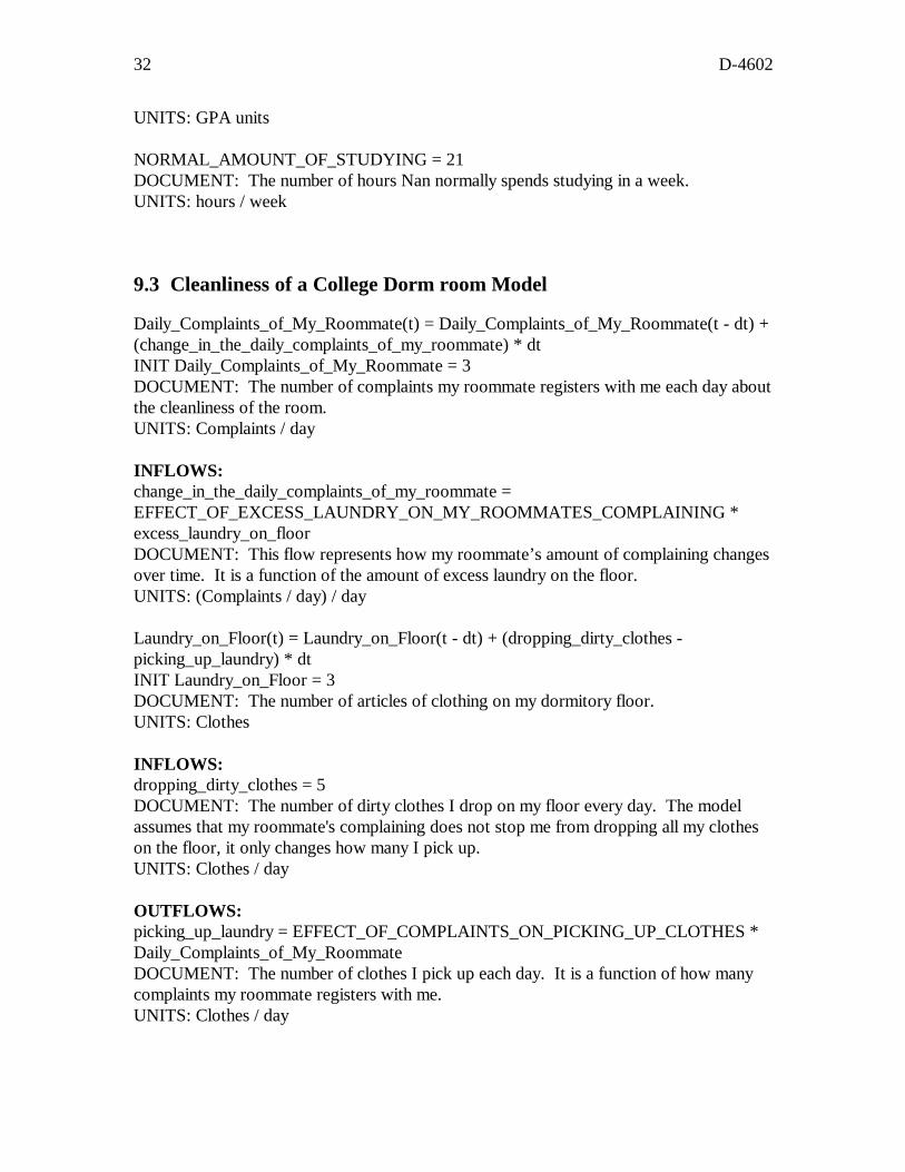
D-4602 1

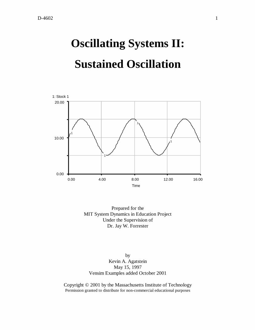
Oscillating Systems II:

Sustained Oscillation

1: Stock 1 20.00

10.00

0.00

1

1

1

1

0.00 4.00 8.00 12.00 16.00

Time

Prepared for theMIT System Dynamics in Education Project

Under the Supervision ofDr. Jay W. Forrester

byKevin A. Agatstein

May 15, 1997Vensim Examples added October 2001

Copyright © 2001 by the Massachusetts Institute of Technology Permission granted to distribute for non-commercial educational purposes

7

D-4602 3

Table of Contents

1. ABSTRACT 6

2. INTRODUCTION

3. SUSTAINED OSCILLATION

4. FIRST-ORDER SYSTEMS

4.1 THE RABBIT POPULATION MODEL 94.2 WHY A FIRST-ORDER SYSTEM CANNOT OSCILLATE 10

5. ACADEMIC PERFORMANCE MODEL 12

5.1 DETAILED MODEL BEHAVIOR ANALYSIS 155.2 DEBRIEF OF THE ACADEMIC PERFORMANCE MODEL 19

6. CLEANLINESS OF A COLLEGE DORM ROOM MODEL 20

6.1 DETAILED MODEL BEHAVIOR ANALYSIS 236.2 DEBRIEF OF THE CLEANLINESS OF A COLLEGE DORM ROOM MODEL 26

7. WHY SECOND-ORDER SYSTEMS CAN OSCILLATE 27

8. CONCLUSION

9. APPENDIX

9.1 FIRST-ORDER RABBIT POPULATION MODEL 299.2 ACADEMIC PERFORMANCE MODEL 309.3 CLEANLINESS OF A COLLEGE DORM ROOM MODEL 32

9. VENSIM EXAMPLES 34

7

9

28

29

6 D-4602

1. Abstract

Oscillating Systems II: Sustained Oscillation is the second paper in a series

dedicated to understanding oscillation. Please read Generic Structures in Oscillating

Systems I,1 before continuing with this paper. This paper assumes knowledge of

STELLA2 software, as well as simple system dynamics structures such as positive and

negative feedback, exponential growth, S-shaped growth, and oscillation.

Oscillating Systems II: Sustained Oscillations will examine the structural features

that allow for sustained oscillation. First, this paper will analyze a simple first-order

system that cannot oscillate in order to develop structural criteria for oscillation. Then, by

studying two different models, an Academic Performance Model of a college student and

the Cleanliness of a College Dorm Room Model, the causes of oscillation will be analyzed.

1Celeste V. Chung, 1994. Generic Structures in Oscillating Systems I (D-4426-1), System Dynamics inEducation Project, System Dynamics Group, Sloan School of Management, Massachusetts Institute ofTechnology, June 17, 25 p.2 STELLA is a registered trademark of High Performance Systems, Inc.

D-4602 7

2. Introduction

Oscillating systems are abundant in nature: a person's sleep-wake patterns, the

number of solar sunspots, the national economy, the pendulum on a grandfather clock, to

name but a few. While the average person observes oscillating systems throughout his

life, understanding why the systems exhibit the oscillating behavior mode is a significant

intellectual undertaking. However, once one understands why a particular system

oscillates, he can transfer that knowledge to many other oscillating systems. The purpose

of this paper is to explore in great detail two simple oscillating systems, and from them

develop an intimate understanding of oscillation and its causes.

3. Sustained Oscillation

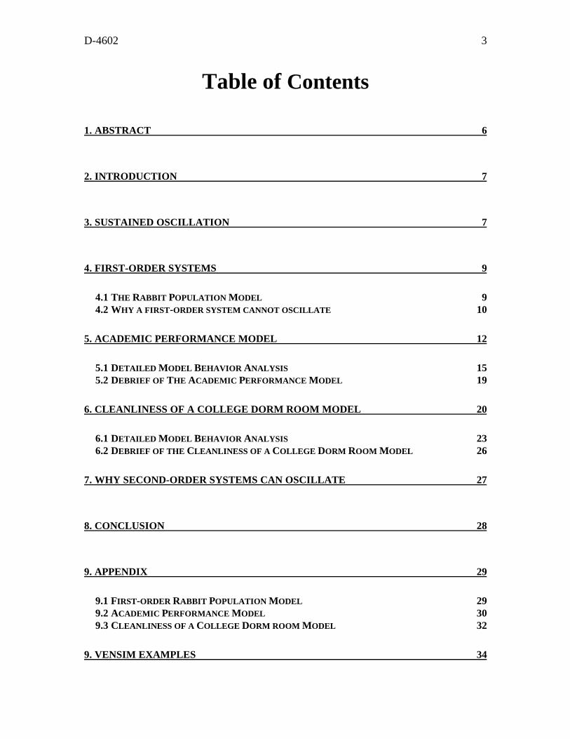
Oscillation refers to a behavior in which the values of the stocks vary around some

average value in a repeating pattern.3 Figure 1 plots the behavior of a stock exhibiting

oscillation over the course of 12 time units. Period

Peak1: Stock 10.00

5.00

0.00

Figure 1: An example of sustained oscillation

0.00 3.00 6.00 9.00 12.00

Time

1

1

1

1

Trough

Period

8 D-4602

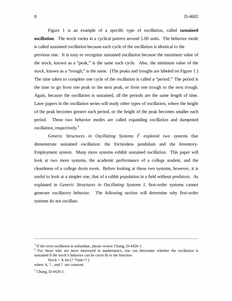
Figure 1 is an example of a specific type of oscillation, called sustained

oscillation. The stock varies in a cyclical pattern around 5.00 units. The behavior mode

is called sustained oscillation because each cycle of the oscillation is identical to the

previous one. It is easy to recognize sustained oscillation because the maximum value of

the stock, known as a “peak,” is the same each cycle. Also, the minimum value of the

stock, known as a “trough,” is the same. (The peaks and troughs are labeled on Figure 1.)

The time taken to complete one cycle of the oscillation is called a “period.” The period is

the time to go from one peak to the next peak, or from one trough to the next trough.

Again, because the oscillation is sustained, all the periods are the same length of time.

Later papers in the oscillation series will study other types of oscillation, where the height

of the peak becomes greater each period, or the height of the peak becomes smaller each

period. These two behavior modes are called expanding oscillation and dampened

oscillation, respectively.4

Generic Structures in Oscillating Systems I5 explored two systems that

demonstrate sustained oscillation: the frictionless pendulum and the Inventory-

Employment system. Many more systems exhibit sustained oscillation. This paper will

look at two more systems, the academic performance of a college student, and the

cleanliness of a college dorm room. Before looking at those two systems, however, it is

useful to look at a simpler one, that of a rabbit population in a field without predators. As

explained in Generic Structures in Oscillating Systems I, first-order systems cannot

generate oscillatory behavior. The following section will determine why first-order

systems do not oscillate.

3 If the term oscillation is unfamiliar, please review Chung, D-4426-1.4 For those who are more interested in mathematics, one can determine whether the oscillation issustained if the stock’s behavior can be curve fit to the function:

Stock = A sin (? *time+? ) where A, ? , and ? are constant. 5 Chung, D-4426-1.

D-4602 9

4. First-order Systems

4.1 The Rabbit Population Model6

The model of “rabbits in a field” is a classic model often used to introduce system

dynamics modeling students to the behavior of S-shaped growth. The only stock in the

model is the “Rabbit Population” in a given-sized field. As one familiar with population

models would predict, the “Rabbit Population” grows exponentially at first. The simple

positive feedback loop of rabbit births leading to more rabbits, which in turn leads to more

rabbit births, causes the exponential growth. Eventually, the “Rabbit Population” will

begin to approach the “carrying capacity”7 of the field. The behavior of “Rabbit

Population” then switches over to an asymptotic approach to the carrying capacity of the

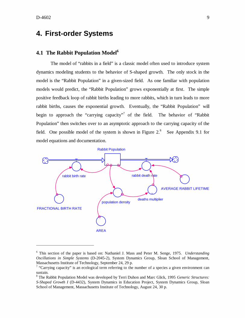
field. One possible model of the system is shown in Figure 2.8 See Appendix 9.1 for

model equations and documentation.

Rabbit Population

rabbit birth rate rabbit death rate

FRACTIONAL BIRTH RATE

population density

~

deaths multiplier

AVERAGE RABBIT LIFETIME

AREA

6 This section of the paper is based on: Nathaniel J. Mass and Peter M. Senge, 1975. UnderstandingOscillations in Simple Systems (D-2045-2), System Dynamics Group, Sloan School of Management,Massachusetts Institute of Technology, September 24, 29 p.7 “Carrying capacity” is an ecological term referring to the number of a species a given environment cansustain.8 The Rabbit Population Model was developed by Terri Duhon and Marc Glick, 1995 Generic Structures:S-Shaped Growth I (D-4432), System Dynamics in Education Project, System Dynamics Group, SloanSchool of Management, Massachusetts Institute of Technology, August 24, 30 p.

10 D-4602

Figure 2: Model of a rabbit population in a field

In Figure 2 the “Rabbit Population” increases as a result of the positive feedback

loop between “rabbit birth rate” and “Rabbit Population.” The increase in “Rabbit

Population” in turn increases the “population density,” which increases the “deaths

multiplier.” The “deaths multiplier” table function reflects that as the “population density”

increases, greater competition develops among the rabbits for food and water. The

increase in the “deaths multiplier” causes the rabbit death loop, a negative feedback loop,

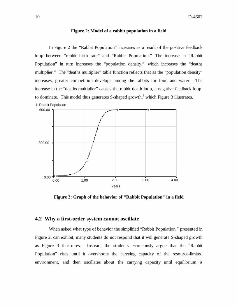
to dominate. This model thus generates S-shaped growth,9 which Figure 3 illustrates.

1: Rabbit Population 600.00

300.00

0.00

1 1

1

1

0.00 1.00 2.00 3.00 4.00

Years

Figure 3: Graph of the behavior of “Rabbit Population” in a field

4.2 Why a first-order system cannot oscillate

When asked what type of behavior the simplified “Rabbit Population,” presented in

Figure 2, can exhibit, many students do not respond that it will generate S-shaped growth

as Figure 3 illustrates. Instead, the students erroneously argue that the “Rabbit

Population” rises until it overshoots the carrying capacity of the resource-limited

environment, and then oscillates about the carrying capacity until equilibrium is

D-4602 11

established. Analysis of the model shows it is impossible for the “Rabbit Population” to

overshoot the carrying capacity. To prove that overshoot is impossible, incorrectly

assume that the rabbit population did in fact overshoot the carrying capacity of the field.

The overshoot and subsequent decline in the “Rabbit Population” incorrectly predicted by

the students is shown in Figure 4. 1: Rabbit Population

1000.00

500.00

0.00

1

1

1 1

0.00 3.00 6.00 9.00 12.00 Years

Figure 4: Erroneous prediction of the behavior of the Rabbit Population Model

On the initial rise, the “rabbit birth rate” exceeds the “rabbit death rate,” and the

“Rabbit Population” grows. As the limited space and resources are used, the effect of

crowding becomes significant, and the “rabbit death rate” gradually approaches the “rabbit

birth rate.” Thus, the “Rabbit Population” is growing more and more slowly. If the

overshoot of the carrying capacity is to occur, the “rabbit birth rate” and “rabbit death

rate” must be equal momentarily. The point when the flows are equal is the very peak of

the population curve, and is indicated by an oval on the graph in Figure 4. However, if the

“Rabbit Population” is in temporary equilibrium, nothing can move it away from

equilibrium. The “rabbit birth rate” and the “rabbit death rate,” the only two flows to and

from the “Rabbit Population” stock, only vary if the “Rabbit Population” varies. All the

9 If S-shaped growth is unfamiliar please review Duhon and Glick, D-4432.

12 D-4602

other terms in the rate equations are constant.10 Moreover, the “Rabbit Population” stock

can only change if the flows into it, the “rabbit birth rate” and “rabbit death rate,” are not

equal. Once the “rabbit birth rate” and “rabbit death rate” are equal, which is the case at

the oval on Figure 4, nothing can alter the value of the stock. Thus, nothing can alter the

value of the two flows in the system. Because the balance cannot be tipped, the system is

locked into equilibrium. The system exhibits the S-shaped growth behavior shown in

Figure 3— NOT the overshoot of equilibrium displayed in Figure 4.

If the “Rabbit Population” system is to deviate from its equilibrium point as

represented by the oval on Figure 4, another variable must continue to change even if the

“Rabbit Population” is momentarily unchanging. The additional variable can be a

changing food or water supply, a predator population, or some other environmental

factor. However, if the variable is to drive the system out of equilibrium, the variable must

not be a function only of the “Rabbit Population.” For example, if an auxiliary variable

affecting the “rabbit birth rate” was solely a function of “Rabbit Population,” it would not

be able to disrupt the temporary equilibrium and generate oscillation.11 Therefore, another

stock-and-flow structure must exist to change the “rabbit birth rate” or “rabbit death rate”

to make the system oscillate. Thus, the “Rabbit Population” example of a first-order, non-

oscillating system shows that a second stock is required for oscillation.

Now, by looking at two second-order systems (systems with two stocks each), this

paper will show two or more stocks are required for oscillation. The first system is a

college student’s academic performance.

5. Academic Performance Model

The first example of an oscillating system this paper will study is Nan’s Grade

Point Average (GPA) over the course of a year. Nan is a college student who hopes to

devote time to her studies as well as to athletics and her social life. As a result she has a

desired goal of graduating with a respectable 3.5 GPA out of a possible 4.0. When Nan’s

grades fall below 3.5, she increases the amount of studying she does each evening. When

10 See equations in Appendix 9.1.

D-4602 13

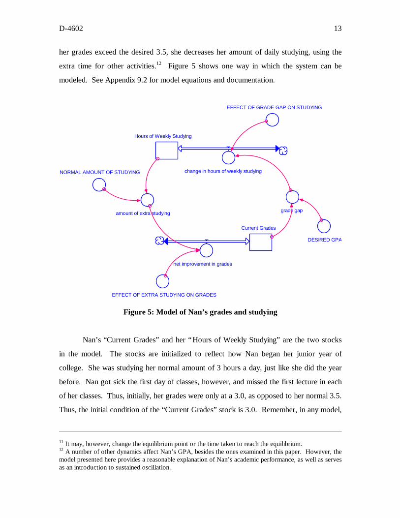
her grades exceed the desired 3.5, she decreases her amount of daily studying, using the

extra time for other activities.12 Figure 5 shows one way in which the system can be

modeled. See Appendix 9.2 for model equations and documentation.

EFFECT OF GRADE GAP ON STUDYING

Hours of Weekly Studying

change in hours of weekly studyingNORMAL AMOUNT OF STUDYING

amount of extra studying

Current Grades

net improvement in grades

grade gap

DESIRED GPA

EFFECT OF EXTRA STUDYING ON GRADES

Figure 5: Model of Nan’s grades and studying

Nan’s “Current Grades” and her “Hours of Weekly Studying” are the two stocks

in the model. The stocks are initialized to reflect how Nan began her junior year of

college. She was studying her normal amount of 3 hours a day, just like she did the year

before. Nan got sick the first day of classes, however, and missed the first lecture in each

of her classes. Thus, initially, her grades were only at a 3.0, as opposed to her normal 3.5.

Thus, the initial condition of the “Current Grades” stock is 3.0. Remember, in any model,

11 It may, however, change the equilibrium point or the time taken to reach the equilibrium.12 A number of other dynamics affect Nan’s GPA, besides the ones examined in this paper. However, themodel presented here provides a reasonable explanation of Nan’s academic performance, as well as servesas an introduction to sustained oscillation.

14 D-4602

all stocks must have initial conditions, not only because the mathematics dictates it, but

because the stocks define the state of the system. The state of the system must be defined

initially.

Before describing the model’s behavior, it is useful to examine the feedback

relationships in the model. Figure 5 shows that as “Current Grades” go down, the “grade

gap” goes up. As the “grade gap” goes up, the “change in hours of weekly studying” goes

up. Because “change in hours of weekly studying” is an inflow to the “Hours of Weekly

Studying” stock, the stock begins to fill more quickly. As “Hours of Weekly Studying”

increases, the “amount of extra studying” also increases. As Nan puts in more and more

extra studying, her “net improvement in grades” begins to rise, increasing her “Current

Grades” over time. Thus, as Nan’s “Current Grades” fall, she puts in more studying, and

her “Current Grades” eventually rise. The only feedback loop in the model is a negative

feedback loop. When the model is simulated, it should demonstrate a behavior

characteristic of a negative feedback loop.

It is also important to notice how each stock affects the flow into the other stock.

As explained by the Rabbit Population Model in the previous section of the paper, two

stocks are required for oscillatory behavior. Nan’s “Current Grades” influence her

“change in hours of weekly studying,“ and Nan’s “Hours of Weekly Studying” affect her

“net improvement in grades.” Structures similar to the Academic Performance Model

appeared in Generic Structures in Oscillating Systems I.13 Thus, it is not surprising that

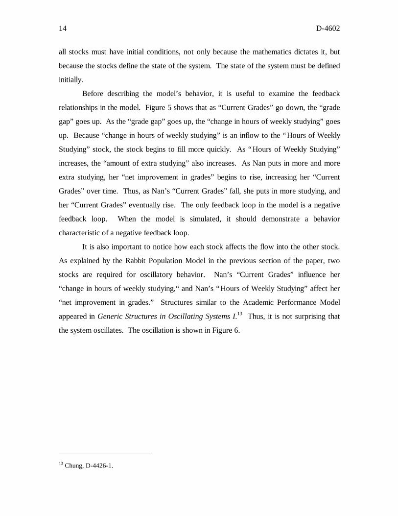
the system oscillates. The oscillation is shown in Figure 6.

13 Chung, D-4426-1.

D-4602 15

1: Current Grades (GPA Units) 2: Hours of Weekly Studying (Hours / week) 1: 4.00 2: 28.00

1: 3.50 2: 21.00

Desired GPA

2

1

2

1

1

2 1 2

1: 3.00 2: 14.00

0.00 13.00 26.00 39.00 52.00

Weeks

Figure 6: Behavior of the Academic Performance Model

Note that the oscillation is sustained because the height of all the peaks is the same, the

height of all the troughs is the same, and the period for each cycle of the oscillation is the 14same.

5.1 Detailed Model Behavior Analysis

The next step in studying the system is to explain why the system demonstrates the

behavior mode of sustained oscillation. The analysis of the model’s behavior will focus on

one period of the system’s oscillation. By studying one period, the whole behavior pattern

can be understood, because each subsequent period is identical to the first one. Figure 7

shows the graph of the stocks and their respective flows of the model during the first

period.

14 For running this model it is recommended that you use the “Runge-Kutta 4” method of integration. To do this in Stella® select RK4 under the “Time Specs...” window that can be opened from the “Run” pull down menu. If the solution interval (DT) is set small enough relative to the time constants of the model, it does not make a great deal of difference what method of integration you use. The graphs look nicer, however, when RK4 is used because the oscillation repeats itself more identically than with Euler’s Method.

16 D-4602

1: Current Grades 2: Hours of Weekly Studying (GPA units) (Hours / week)

1: 4.00 2: 28.00

1: 3.50 2: 21.00

1: 3.00 2: 14.00

2

1

2

1

2 1

2

1 The Stocks

0.00 6.00 12.00 18.00 24.00 Weeks

1: net improvement in grades 2: change in hours of weekly studying (GPA units / week) (Hours / week / week)

1: 0.20 2: 1.50

1: 0.00 2: 0.00

1: -0.202: -1.50

2 1

2

1

2

1

The Flows 2 1

0.00 6.00 12.00 18.00 24.00 Weeks

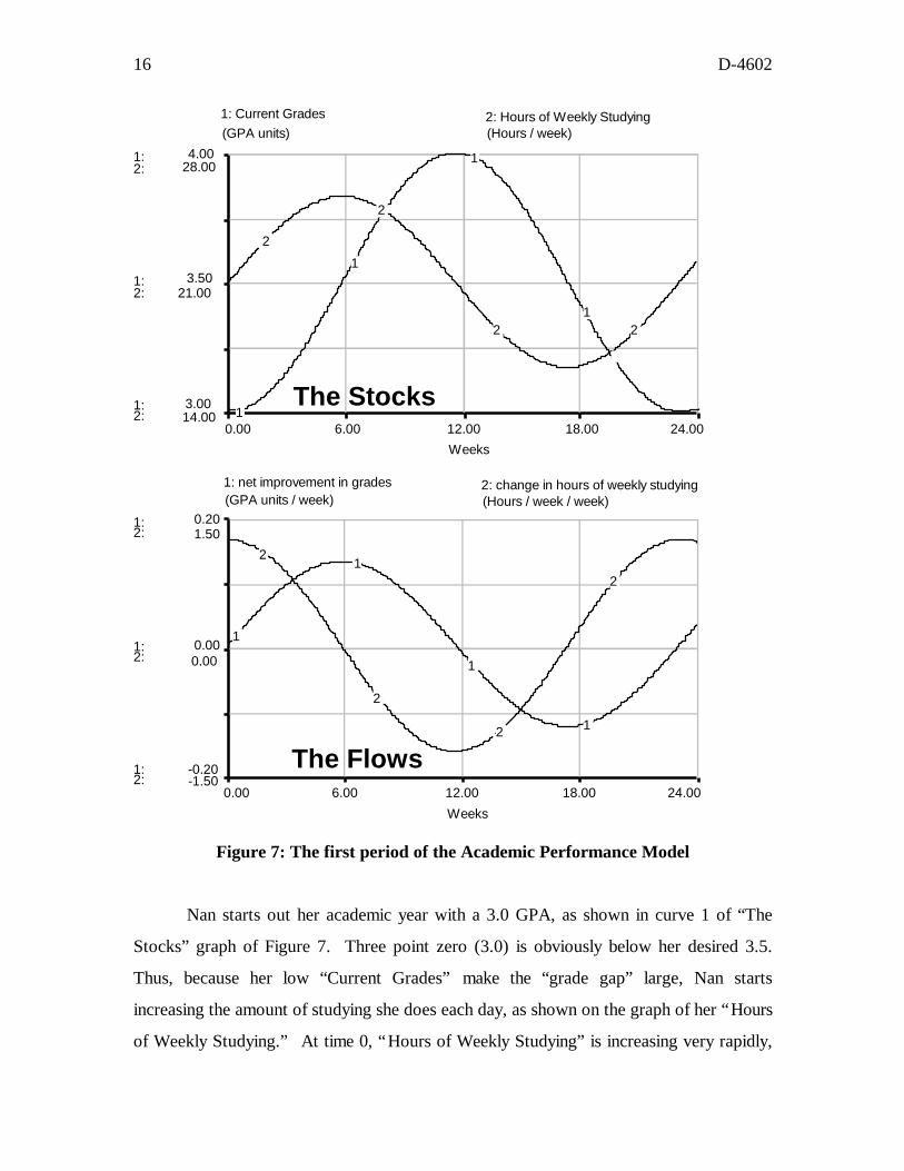
Figure 7: The first period of the Academic Performance Model

Nan starts out her academic year with a 3.0 GPA, as shown in curve 1 of “The

Stocks” graph of Figure 7. Three point zero (3.0) is obviously below her desired 3.5.

Thus, because her low “Current Grades” make the “grade gap” large, Nan starts

increasing the amount of studying she does each day, as shown on the graph of her “Hours

of Weekly Studying.” At time 0, “Hours of Weekly Studying” is increasing very rapidly,

D-4602 17

and thus the graph of the “change in hours of weekly studying” is at its highest point. As

time passes, Nan’s “Current Grades” begin to improve because of her extra studying. As

her “Current Grades” increase, the gap between her “DESIRED GPA” and her “Current

Grades” shrinks. Nan continues to increase her “Hours of Weekly Studying” because she

is still below her “DESIRED GPA.” However, she increases her amount of studying by

less and less as the gap between her “Current Grades” and her “DESIRED GPA” shrinks.

By 6 weeks, when she finally reaches her “DESIRED GPA,” she is no longer increasing

her “Hours of Weekly Studying.” Notice that at week 6, her “change in hours of weekly

studying” is zero hours in a week per week.

So far, the system does not demonstrate anything particularly new. Nan’s grades

were below what she wanted them to be, so she increased her studying, a great deal at

first, then less and less, until she eventually closed the gap and reached her goal. When

she finally reached her goal, she stopped increasing her amount of studying. The feedback

relationship described is an example of a negative feedback loop. The system oscillates

because at week 6, when her “Current Grades” are the desired 3.5, all the studying Nan

put in up until that point then causes her “Current Grades” to rise past the goal of 3.5.

Remember, by week 6 Nan has been studying 26 hours a week, so she is going to do well

on her quizzes and exams for the next few weeks. In fact, her “net improvement in

grades,” which is the flow into the “Current Grades” stock, is at its highest. Her “net

improvement in grades” is at its highest because Nan at week 6 has been over the last six

weeks continually increasing her weekly amount of studying. Thus, by week 6, she is

putting in the most hours a week in studying, almost 26 hours weekly! All the studying

means that her “Current Grades” are rising most rapidly when she is at the goal.

At week 6, when Nan reaches her academic goal, she is no longer increasing her

“Hours of Weekly Studying.” Thus, exactly at week 6 the “change in hours of weekly

studying” is zero. Had Nan’s academic performance been a first-order system, the

negative feedback loop would have reached its goal and permanent equilibrium would

have been established. To Nan’s delight, however, her “Current Grades” continue to rise

past her goal. While she is happy about her continually rising grades, Nan decides to cut

back on her amount of time studying so that she is free to do other things she enjoys.

18 D-4602

Immediately after week 6, Nan’s “change in hours of weekly studying” becomes negative.

Her “Current Grades,” however, still continue to rise from all the studying she had done

before then. Her “Current Grades” do rise more and more slowly though because the rise

is no longer reinforced by an increase in her “Hours of Weekly Studying.” Thus, the “net

improvement in grades” is positive, but begins to head back down towards zero GPA units

per week. As Nan’s “Current Grades” continue to rise, Nan feels more and more like

using her time elsewhere, and her “Hours of Weekly Studying” continue to decrease.

As everyone knows, if a student keeps cutting back on studying, her grades will

eventually fall. The same holds true for Nan as well. At week 12, Nan’s “Current

Grades” have reached 4.0, and she is back down to studying 21 hours a week.

Remember, Nan’s “Current Grades” have been growing, even though she has been cutting

back on her amount of studying because of the extra work done initially. Her “Current

Grades,” however, have been growing slower and slower since week 6 when she was

studying the maximum amount. Nan is unbelievably happy— she has a great GPA, and is

studying a mere 21 hours a week.

After week 12, things begin to turn sour. For the previous six weeks Nan has been

cutting back on her studying, so her “Current Grades” are beginning to fall. Because

Nan’s GPA is still above her goal she continues reducing her “Hours of Weekly

Studying.” The reduction in her “Hours of Weekly Studying” continues for the entire time

between week 12 and week 18. She does, however, reduce her studying less and less each

week as her GPA falls closer and closer to her goal.

By week 18, Nan’s “Current Grades” have fallen from their peak at 4.0 and have

reached her “DESIRED GPA” of 3.5. If the system had been a first-order system, like the

Rabbit Population system looked at in section 4, once the system reached its goal

equilibrium would be established. Unfortunately for Nan, her academic performance is not

a first-order system. Nan’s “Current Grades” continue to fall after week 18, and thus fall

below her goal. Nan’s “Current Grades” fall below the goal because since week 6, when

her GPA was high, she was studying less than average. After week 18, when Nan’s

“Current Grades” fall below her goal, she increases her “Hours of Weekly Studying.”

However, the increase in studying takes time to increase her “Current Grades” the desired

D-4602 19

amount. Remember, studying does not directly increase her “Current Grades.” Instead,

studying increases her “net improvement in grades,” the flow into her “Current Grades”

stock. The increase in her “net improvement in grades” does increase her grades over

time.

Immediately after week 18, Nan’s GPA will continue to fall no matter what Nan

does. Eventually, the studying she does will reverse the system, and her “Current Grades”

will rise again. In fact, just as when her “Current Grades” were low at week 0, they will

rise again. The time between Nan’s studying and the improvement in her “Current Grades”

will cause her “Current Grades” to overshoot her goal and perpetuate the oscillation.

5.2 Debrief of The Academic Performance Model

The Academic Performance Model demonstrates a great deal about oscillating

systems. As expected from studying the Rabbit Population Model, an oscillating system

requires two stocks. The second stock allows for the first stock to continue to change

even if the first stock was temporarily in its equilibrium position. Specifically, in Nan’s

Academic Performance model, the “Hours of Weekly Studying” change even if Nan’s

“Current Grades” are at the goal value of 3.5 (Nan’s “DESIRED GPA”). Nan’s “Current

Grades” keep increasing because Nan’s “net improvement in grades” is a function of her

“Hours of Weekly Studying,” NOT of her “Current Grades.” Studying Figure 7 closely

will show that the net flow into or out of a stock is greatest when the stock is in its goal

position.15

Another thing to notice about oscillating systems from Nan’s Academic

Performance Model is that oscillating systems have some momentum associated with

them. In a first-order negative feedback loop, the system takes action when a gap exists

between the state of the system and the goal of the system. The system thus approaches

the goal asymptotically. The asymptotic approach can be seen in the Rabbit Population

Model studied earlier. For instance, assume that a hundred rabbits escape from a

15 Later papers in the oscillation series will expose the reader to systems in which sustained oscillation is not exhibited, and dampened and expanding oscillation will occur.

20 D-4602

laboratory and try to live in the field that was originally in equilibrium. Because the

number of rabbits in the field is suddenly greater than the carrying capacity, “rabbit death

rate” increases, and the number of rabbits approaches the carrying capacity of the

environment. Equilibrium is re-established. In Nan’s Academic Performance model, when

Nan’s “Current Grades” are below her goal, she cannot immediately raise her GPA.

Instead, she must increase her amount of studying that will in turn, after a few weeks, raise

her “Current Grades” to her desired level. Unfortunately for Nan, until her “Current

Grades” actually reach the “DESIRED GPA” she does not know to stop increasing her

“Hours of Weekly Studying.” Thus she overstudies, which allows her grades to overshoot

and undershoot her goal GPA, and thus the oscillatory behavior of the model is produced.

Building and experimenting with the model will yield tremendous insights into

oscillation. Try changing the value of the constants and initial conditions of the stocks.

As always when simulating a model, try to understand why changing a certain variable

alters the model’s behavior.

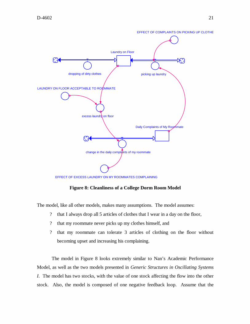
6. Cleanliness of a College Dorm Room Model

Imagine a college dorm room with one very messy roommate (me) who always

drops his dirty clothes on the floor. My very neat roommate always complains about the

untidiness of the room, especially when my dirty clothes spill over to his side of the room.

When the clothes begin to untidy his side of the room, he complains, and I pick up some

of the clothes. His complaining then subsides as the room becomes tidier. When the

complaining subsides, I stop picking up the clothing because I am a slob. As the amount

of laundry on the floor begins to reaccumulate, the number of complaints registered by my

roommate each day increases. The complaints increase my willingness to pick up laundry,

which decreases the amount of clothes on the floor. The increase in the cleanliness of the

room of course reduces his complaining. A model of the system is shown in Figure 8. For

equations and documentation see Appendix, Section 9.3.

D-4602 21

EFFECT OF COMPLAINTS ON PICKING UP CLOTHES

Laundry on Floor

Daily Complaints of My Roommate

change in the daily complaints of my roommate

picking up laundrydropping of dirty clothes

excess laundry on floor

LAUNDRY ON FLOOR ACCEPTABLE TO ROOMMATE

EFFECT OF EXCESS LAUNDRY ON MY ROOMMATES COMPLAINING

Figure 8: Cleanliness of a College Dorm Room Model

The model, like all other models, makes many assumptions. The model assumes:

? that I always drop all 5 articles of clothes that I wear in a day on the floor,

? that my roommate never picks up my clothes himself, and

? that my roommate can tolerate 3 articles of clothing on the floor without

becoming upset and increasing his complaining.

The model in Figure 8 looks extremely similar to Nan’s Academic Performance

Model, as well as the two models presented in Generic Structures in Oscillating Systems

I. The model has two stocks, with the value of one stock affecting the flow into the other

stock. Also, the model is composed of one negative feedback loop. Assume that the

22 D-4602

“Laundry on Floor” increases and thus the “excess laundry on floor” increases. As the

amount of excess clothing on the floor rises, my roommate’s unhappiness increases, and

thus the “change in the daily complaints of my roommate,” the flow into the “Daily

Complaints of My Roommate” stock, also increases. As the flow into a stock increases,

the value of the stock increases as well. Thus the “Daily Complaints of My Roommate”

increases. The increased complaining causes the “picking up laundry” flow to increase.

Because “picking up laundry” is an outflow, the “Laundry on Floor” decreases. Thus, the

model is one negative feedback loop— as the amount of laundry increases, my roommate

complains more, which causes me to pick up more clothes. The amount of laundry on the

floor thus decreases.

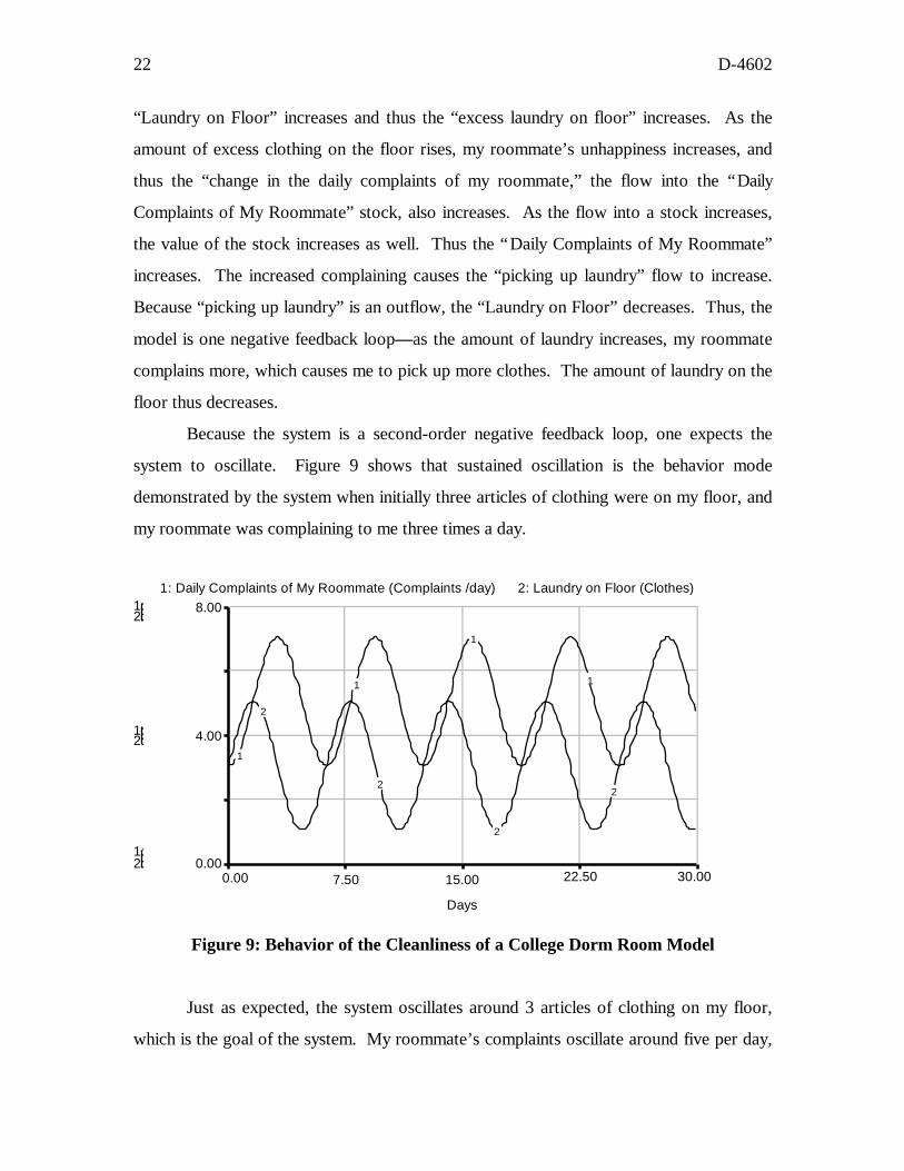
Because the system is a second-order negative feedback loop, one expects the

system to oscillate. Figure 9 shows that sustained oscillation is the behavior mode

demonstrated by the system when initially three articles of clothing were on my floor, and

my roommate was complaining to me three times a day.

1: Daily Complaints of My Roommate (Complaints /day) 2: Laundry on Floor (Clothes) 1:2:

1:2:

1: 2:

8.00

4.00

0.00

1

2

1 1

1

2 2

2

0.00 7.50 15.00 22.50 30.00

Days

Figure 9: Behavior of the Cleanliness of a College Dorm Room Model

Just as expected, the system oscillates around 3 articles of clothing on my floor,

which is the goal of the system. My roommate’s complaints oscillate around five per day,

D-4602 23

which is the number of complaints per day required to keep me picking up as many clothes

as I drop. The initial conditions of the simulation reflect what happened at the start of

February, 1996. Originally, 3 articles of clothes untidied the floor and my roommate was

complaining 3 times a day. Three times a day was less than he normally complains

because he just received a very generous financial aid package from MIT.

It is important to notice that the oscillation is sustained because all the peaks for

each stock are the same height and all the troughs for each stock are the same height. To

explain why the oscillation occurs, one can study the first few days of the system and

recognize that any subsequent behavior is simply a repetition of the initial behavior.

6.1 Detailed Model Behavior Analysis

Figure 10 shows the behavior of the stocks of the system, “Laundry on my Floor”

and “Daily Complaints of My Roommate,” for the first week. Figure 10 also shows the

behavior of the “change in the daily complaints of my roommate” and the “picking up

laundry” flows. “Dropping dirty clothes,” the inflow to “Laundry on Floor,” is constant at

5 clothes per day.

24 D-4602

1: Daily Complaints of my Roommate 2: Laundry on Floor 1: 8.002:

1: 2: 4.00

1: 2: 0.00

1 The Stocks

1

2

1 1

2

2 2

0.00 3.00 6.00 9.00 12.00

Days

1: change in the daily complaints of my roommate 2: picking up laundry

Days

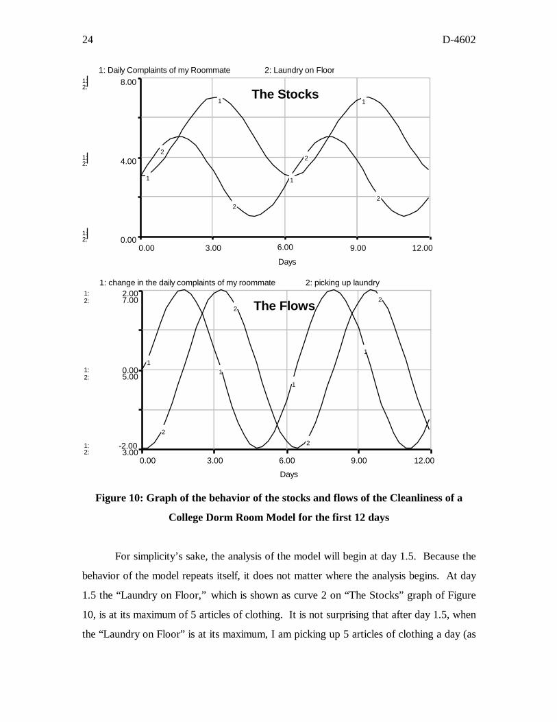
Figure 10: Graph of the behavior of the stocks and flows of the Cleanliness of a

College Dorm Room Model for the first 12 days

For simplicity’s sake, the analysis of the model will begin at day 1.5. Because the

behavior of the model repeats itself, it does not matter where the analysis begins. At day

1.5 the “Laundry on Floor,” which is shown as curve 2 on “The Stocks” graph of Figure

10, is at its maximum of 5 articles of clothing. It is not surprising that after day 1.5, when

the “Laundry on Floor” is at its maximum, I am picking up 5 articles of clothing a day (as

0.00 3.00 6.00 9.00 12.00

1:

1:

1:

2:

2:

2:

-2.00

0.00

2.00

3.00

5.00

7.00

1 1

1

1

2

2

2

2The Flows

D-4602 25

shown on curve 2 of “The Flows” graph of Figure 10). Remember, every day I drop 5

articles of clothing on the floor, so when I am picking up 5, the stock is in temporary

equilibrium. Even though the stock of “Laundry on Floor” is temporarily in equilibrium

(the inflow equal to the outflow), the number of articles of clothing on the floor is greater

than the 3 articles my roommate considers tolerable. Thus, my roommate continues to

increase his number of daily complaints. The increase in complaints is shown on Figure 10

where curve 1 on “The Flows” graph is at positive 2.00 (Complaints/day)/day.

After day 1.5 my roommate’s complaints drive me to pick up more laundry off my

floor. Because picking up laundry is the outflow from the “Laundry on Floor” stock, the

amount of “Laundry on Floor” decreases. My roommate, however, continues to increase

his complaining because more than 3 articles of clothing are on the floor. A little after day

3, I have reduced the amount of laundry on the floor to 3 articles. Thus, at a little after

day 3, my roommate stops increasing his amount of complaining. However, I am still

hearing him complain 7 times a day. Remember, he has only stopped increasing his

amount of complaining, he has NOT stopped complaining. What is interesting is that my

roommate can normally tolerate 3 articles of clothing on the floor. Because he is so mad

at me, however, it takes him time to change his daily number of complaints. Thus, the

amount of laundry on the floor drops below 3 articles of clothing. The seven complaints a

day, the peak of his daily complaints, cause me to continue to pick up more clothes than I

drop. The amount of “Laundry on Floor” continues to fall. The decrease of “Laundry on

Floor” pleases my roommate. He begins softening up on me by reducing his daily

complaints. He is still, at least right after day 3, complaining quite a bit, and I continue to

pick up more clothes than I drop. As my roommate’s number of daily complaints falls, so

does my picking up of my laundry.

By around day 5 the “Laundry on my Floor” is at a minimum of 1 article of

clothing. Between slightly after day 3 and day 4.5, I have been decreasing the amount of

laundry I have been picking up off the floor because my roommate has begun to reduce his

complaining. By day 4.5, I am only picking up 5 articles of clothing a day, which means

that the amount of “Laundry on my Floor” is temporarily in equilibrium again. Because

only 1 article of clothing is on the floor, which is far below the 3 articles my roommate

26 D-4602

finds acceptable, he continues to reduce his amount of complaining. My roommate’s lack

of complaining causes me to continue to reduce my picking up of laundry, and the clothes

begin to reaccumulate on my floor. Eventually, by day 6.0 (actually, slightly after day 6.0)

the amount of “Laundry on Floor” reaches 3 articles and my roommate stops decreasing

his amount of complaining. Because he is complaining so little, I continue not to pick up

as many clothes off the floor as I drop, and my laundry accumulates. The accumulation

continues until my roommate’s complaints reach a high enough level to force me to pick

up more clothes than I drop. As Figure 10 shows, the oscillation perpetuates indefinitely.

6.2 Debrief of the Cleanliness of a College Dorm Room Model

Similar to the Academic Performance Model, the Cleanliness of a College Dorm

Room Model shows an oscillatory pattern.16 One could expect the behavior mode

because the model meets the requirement of being second-order (two stocks), with the

flows into one stock determined by the value of the other stock. For example, the flow

“picking up laundry” is a function of the “Daily Complaints of My Roommate” stock.

Also, the flow “change in the daily complaints of my roommate” is a function of the stock

of “Laundry on Floor.”

Furthermore, one would also expect the system to oscillate because it is a negative

feedback loop. The momentum in the system is that my roommate gets into a good or bad

mood and cannot change his amount of complaining immediately. Thus, when my

roommate is not satisfied with the state of the system, he can start to get more annoyed

and increase his complaining. It takes him about a day to change his amount of

complaining. Because of his inability to change his mood immediately, when finally the

amount of “Laundry on Floor” is acceptable to him, he is already so mad at me that it

takes him time to stop complaining. The time for my roommate to change his mood

causes me to overshoot the equilibrium and continue to pick clothes up faster than I drop

them. The same holds true in the reverse. When the “Laundry on Floor” stock is small

and then reaccumulates so that it reaches 3 articles (the amount acceptable to my

roommate), it immediately overshoots because my roommate is complaining very little. It

D-4602 27

takes time for his mood to change sufficiently to complain enough to keep the laundry on

the floor at his acceptable level. Thus, the momentum in the system always causes the

system to overshoot and undershoot the equilibrium, and thus oscillation occurs.

Again, it is important to build and experiment with the model to gain a strong

intuition as to why the sustained oscillating behavior exists. Try changing the “EFFECT

OF ROOMMATES COMPLAINTS ON PICKING UP CLOTHES” variable in particular.

This variable represents how much of an effect my roommate’s complaining has on my

picking up my clothes off the floor.

7. Why Second-order Systems Can Oscillate

The three systems studied in this paper illustrate some of the structural

requirements of sustained oscillation. The requirements are:

? The system must be a negative feedback loop.

? The system must be at least second-order (have two stocks).

Negative feedback loops always attempt to close the gap between some desired

state of the system and the actual state of the system. For example, the negative feedback

loop showed in the Rabbit Population Model over time closed the gap between the

“Rabbit Population” and the carrying capacity of the field. Also, the negative feedback

loop in the Cleanliness of a College Dorm Room Model attempted over time to close the

gap between the amount of laundry on the floor and the amount of laundry my roommate

considered acceptable. Earlier papers in Road Maps showed how first-order (one stock)

negative feedback loops generate asymptotic growth, also known as goal-seeking

behavior.17 The goal-seeking behavior occurs because the system realizes that a gap exists

between the desired state and actual state, and adjusts the rates of the system. The system

then immediately recompares the actual state of system to the goal, and readjusts the rates

16 It also shows how much of a slob and a rotten roommate I am.17 Stephanie Albin, 1996. Generic Structures: Negative Feedback Loops (D-4475-1), System Dynamicsin Education Project, System Dynamics Group, Sloan School of Management, Massachusetts Institute ofTechnology, May 28, 28 pp.

28 D-4602

accordingly. For example, if the initial “Rabbit Population” was larger than the carrying

capacity, goal-seeking behavior would result. The “rabbit death rate” would increase, and

thus the “Rabbit Population” would shrink, which then would decrease the “rabbit death

rate.”

Now, for comparison, consider the model of Nan’s academic performance. When

Nan’s “Current Grades” are too low, she cannot simply improve her “Current Grades” a

proportional amount immediately. Thus, the second-order system is different from the

first-order Rabbit Population Model. In the Rabbit Population Model, should the number

of rabbits exceed the carrying capacity, more rabbits would die than would be born. The

stock-and-flow structure of the Academic Performance Model, shown in Figure 5,

contains no direct link between “grade gap” and “net improvement in grades.” Instead,

the corrective action the system takes is to increase Nan’s “Hours of Weekly Studying.”

The increase of studying raises her “Current Grades,” but not in the same fashion as in a

first-order feedback loop. The oscillation occurs because Nan keeps increasing her

studying until she reaches her goal. She overshoots her “DESIRED GPA” because she

overstudied. When Nan’s “Current Grades” stock is at its desired value, all the studying

she put in up to then increased her “Hours of Weekly Studying” stock to almost 28 hours

a week. Nan’s large amount of studying means that her “net improvement in grades,” the

flow into the “Current Grades” stock, is large. Thus, Nan overshoots the goal of the

system (Nan's “DESIRED GPA”) and the system is able to oscillate. Nan later

undershoots her “DESIRED GPA” for the same reason— because of the momentum in the

system when one stock is at its goal value, the other stock drives it out of equilibrium. As

learned from studying the Rabbit Population Model, a second stock allows for oscillation.

The second stock can continue to change the system even if one of the stocks is at its goal

value.

8. Conclusion

Through studying the first-order system of a rabbit population in a field, it was

determined that for a system to oscillate, the system must be a negative feedback loop

with at least two stocks. Also, the flows into one stock must be a function of the other

D-4602 29

stock in the model. If each flow was only a function of the stock it fed into or out of, the

system could not move from equilibrium once it was established. For example, the

“Rabbit Population” was stable when it reached its maximum in the first model of this

paper because the “rabbit birth rate” and “rabbit death rate” were only functions of the

“Rabbit Population.” Once the “Rabbit Population” reached the carrying capacity of the

environment, nothing could move the system from equilibrium. In Nan’s Academic

Performance Model, however, when Nan’s “Current Grades” were in equilibrium (equal

to her “DESIRED GPA,”) the amount of studying she had done previously caused her

“Current Grades” to move away from equilibrium. Lastly, the notion that all models must

have a set of initial conditions for the stocks was reiterated.

Future papers in Road Maps will expose the reader to more complex types of

oscillation, both expanding and dampened. Oscillating Systems II: Sustained Oscillation

outlines the basic causes of sustained oscillation. The reader’s understanding will grow as

he experiments with the models presented in this paper, as well as develops oscillating

models from scratch. The reader is encouraged to build the models presented here and

study how their behavior changes as the various parameters and initial conditions of the

stocks are altered. It is important to understand the mechanism of sustained oscillation

before studying more complex oscillatory behaviors.

9. Appendix

The following are the equations and the documentation of the three models presented in

this paper:

9.1 First-order Rabbit Population Model

Rabbit_Population(t) = Rabbit_Population(t - dt) + (rabbit_birth_rate - rabbit_death_rate) * dt INIT Rabbit_Population = 2 DOCUMENT: The number of rabbits in the field. UNITS: Rabbits

INFLOWS:

30 D-4602

rabbit_birth_rate = Rabbit_Population * FRACTIONAL_BIRTH_RATE DOCUMENT: The number of rabbits born each year. UNITS: Rabbits / year

OUTFLOWS: rabbit_death_rate = (Rabbit_Population / AVERAGE_RABBIT_LIFETIME) *deaths_multiplierDOCUMENT: The number of rabbits dying each year.UNITS: Rabbits / year

AREA = 1DOCUMENT: The size of the field the rabbits are living in.UNITS: Acres

AVERAGE_RABBIT_LIFETIME = 4DOCUMENT: The average life span of a rabbit living in an uncrowded environment.UNITS: Years

FRACTIONAL_BIRTH_RATE = 5.0DOCUMENT: The number of rabbits born each year into the population per rabbit in thepopulation.UNITS: Fraction / year

population_density = Rabbit_Population / AREADOCUMENT: The number of rabbits per acre of field.UNITS: Rabbits / acre

deaths_multiplier = GRAPH(population_density)(0.00, 1.00), (100, 2.50), (200, 5.00), (300, 7.75), (400, 10.75), (500, 15.25), (600,20.25), (700, 26.50), (800, 34.75), (900, 43.00), (1000, 50.00)DOCUMENT: Deaths multiplier is a multiplication factor which depends uponPOPULATION DENSITY. It converts density to a factor that affects the number ofrabbit deaths (i.e., it makes the rabbit death rate a function of POPULATION DENSITY).The deaths multiplier reflects that the more dense the rabbit population is, the morecompetition there is for food and water, so the more rabbits die.UNITS: dimensionless

9.2 Academic Performance Model

Current_Grades(t) = Current_Grades(t - dt) + (net_improvement_in_grades) * dt INIT Current_Grades = 3.0 DOCUMENT: Nan's academic performance at any given time.

D-4602 31

UNITS: GPA units

INFLOWS: net_improvement_in_grades = amount_of_extra_studying * EFFECT_OF_EXTRA_STUDYING_ON_GRADES DOCUMENT: This is the change in Nan's grades as a result of studying more or less than her normal amount. UNITS: GPA units / week

Hours_of_Weekly_Studying(t) = Hours_of_Weekly_Studying(t - dt) + (change_in_hours_of_weekly_studying) * dt INIT Hours_of_Weekly_Studying = 21 DOCUMENT: The number of hours Nan spends per week studying. The initial value of 21 hours per week corresponds to 3 hours per night. UNITS: hours / week

INFLOWS: change_in_hours_of_weekly_studying = grade_gap *EFFECT_OF_GRADE_GAP_ON_STUDYINGDOCUMENT: The number of hours by which Nan increases or decreases her amount ofstudying based on her current academic performance.UNITS: (hours / week) / week

amount_of_extra_studying = Hours_of_Weekly_Studying ­NORMAL_AMOUNT_OF_STUDYINGDOCUMENT: The number of hours in a week Nan spends studying above her normalamount.UNITS: hours / week

DESIRED_GPA = 3.5DOCUMENT: The GPA Nan wants.UNITS: GPA units

EFFECT_OF_EXTRA_STUDYING_ON_GRADES = 0.0285DOCUMENT: The amount by which Nan's academic performance is increased one extrahour.UNITS: GPA units / hour

EFFECT_OF_GRADE_GAP_ON_STUDYING = 2.45DOCUMENT: The amount by which Nan increases her weekly studying when she isbelow her desired GPA by 1.0 points.UNITS: [(Hours / week) / week] / GPA units

grade_gap = DESIRED_GPA - Current_GradesDOCUMENT: The difference between Nan's desired and actual GPA.

32 D-4602

UNITS: GPA units

NORMAL_AMOUNT_OF_STUDYING = 21 DOCUMENT: The number of hours Nan normally spends studying in a week. UNITS: hours / week

9.3 Cleanliness of a College Dorm room Model

Daily_Complaints_of_My_Roommate(t) = Daily_Complaints_of_My_Roommate(t - dt) + (change_in_the_daily_complaints_of_my_roommate) * dt INIT Daily_Complaints_of_My_Roommate = 3 DOCUMENT: The number of complaints my roommate registers with me each day about the cleanliness of the room. UNITS: Complaints / day

INFLOWS: change_in_the_daily_complaints_of_my_roommate =EFFECT_OF_EXCESS_LAUNDRY_ON_MY_ROOMMATES_COMPLAINING *excess_laundry_on_floorDOCUMENT: This flow represents how my roommate’s amount of complaining changesover time. It is a function of the amount of excess laundry on the floor.UNITS: (Complaints / day) / day

Laundry_on_Floor(t) = Laundry_on_Floor(t - dt) + (dropping_dirty_clothes ­picking_up_laundry) * dtINIT Laundry_on_Floor = 3DOCUMENT: The number of articles of clothing on my dormitory floor.UNITS: Clothes

INFLOWS: dropping_dirty_clothes = 5 DOCUMENT: The number of dirty clothes I drop on my floor every day. The model assumes that my roommate's complaining does not stop me from dropping all my clothes on the floor, it only changes how many I pick up. UNITS: Clothes / day

OUTFLOWS: picking_up_laundry = EFFECT_OF_COMPLAINTS_ON_PICKING_UP_CLOTHES * Daily_Complaints_of_My_Roommate DOCUMENT: The number of clothes I pick up each day. It is a function of how many complaints my roommate registers with me. UNITS: Clothes / day

D-4602 33

EFFECT_OF_EXCESS_LAUNDRY_ON_MY_ROOMMATES_COMPLAINING = 1 DOCUMENT: This constant reflects how my roommate increases his complaining based on the addition of one more article of clothing to the floor. UNITS: ((Complaints / day) / day) / Clothes

EFFECT_OF_ COMPLAINTS_ON_PICKING_UP_CLOTHES = 1 DOCUMENT: This variable is the number of extra clothes I will pick up each day if my roommate increases his complaining by one complaint per day. UNITS: (Clothes / day) / (Complaint / day), or more simply, Clothes / Complaints

excess_laundry_on_floor = Laundry_on_Floor ­LAUNDRY_ON_FLOOR_ACCEPTABLE_TO_ROOMMATE DOCUMENT: This variable is the difference between the number of articles of clothing on my floor and the number of articles acceptable to my roommate. UNITS: Clothes

LAUNDRY_ON_FLOOR_ACCEPTABLE_TO_ROOMMATE = 3 DOCUMENT: This is the number of clothes on the floor my roommate finds acceptable (because they don't spill over onto his side of the room). UNITS: Clothes

Vensim Examples: Oscillating Systems II:

Sustained OscillationBy Aaron Diamond

March 2000

34 D-4602

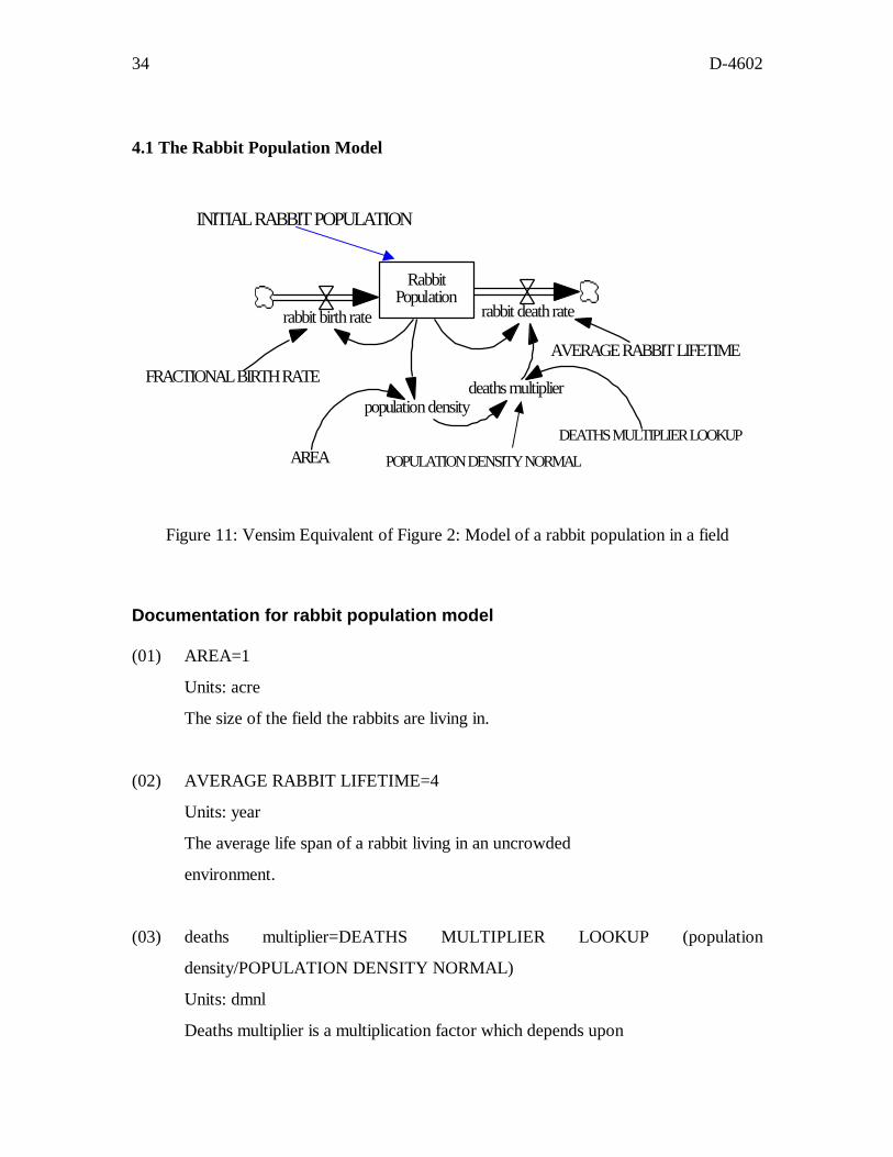
4.1 The Rabbit Population Model

INITIAL RABBIT POPULATION

Rabbit Population

rabbit birth rate rabbit death rate

FRACTIONAL BIRTH RATE AVERAGE RABBIT LIFETIME

deaths multiplier population density

AREA DEATHS MULTIPLIER LOOKUP

POPULATION DENSITY NORMAL

Figure 11: Vensim Equivalent of Figure 2: Model of a rabbit population in a field

Documentation for rabbit population model

(01) AREA=1

Units: acre

The size of the field the rabbits are living in.

(02) AVERAGE RABBIT LIFETIME=4

Units: year

The average life span of a rabbit living in an uncrowded

environment.

(03) deaths multiplier=DEATHS MULTIPLIER

density/POPULATION DENSITY NORMAL)

Units: dmnl

LOOKUP (population

Deaths multiplier is a multiplication factor which depends upon

D-4602 35

POPULATION DENSITY. It converts density to a factor that affects

the number of rabbit deaths (i.e., it makes the rabbit death

rate a function ofPOPULATION DENSITY). The deaths multiplier

reflects that the more dense the rabbit population is, the more

competition there is for food and water, so the more rabbits die.

(04) DEATHS MULTIPLIER LOOKUP= ([(0,0),(10,60)], (0,1), (100,2.5), (200,5),

(300,7.75),(400,10.75),(500,15.25),(600,20.25),(700,26.5),(800,34.75),(900,43),

(1000,50))

Units: dmnl

(05) FINAL TIME = 4

Units: year

The final time for the simulation.

(06) FRACTIONAL BIRTH RATE=5

Units: 1/year

The number of rabbits born each year into the population per

rabbit in the population.

(07) INITIAL RABBIT POPULATION=2

Units: rabbits

(08) INITIAL TIME = 0

Units: year

The initial time for the simulation.

(09) population density=Rabbit Population/AREA

Units: rabbits/acre

The number of rabbits per acre of field.

36 D-4602

(10) POPULATION DENSITY NORMAL=1

Units: rabbits/acre

(11) rabbit birth rate=Rabbit Population*FRACTIONAL BIRTH RATE

Units: rabbits/year

The number of rabbits born each year.

(12) rabbit death rate=(Rabbit Population/AVERAGE RABBIT LIFETIME)*deaths

multiplier

Units: rabbits/year

The number of rabbits dying each year.

(13) Rabbit Population= INTEG (rabbit birth rate-rabbit death rate, INITIAL RABBIT

POPULATION)

Units: rabbits

The number of rabbits in the field.

(14) SAVEPER =TIME STEP

Units: year

The frequency with which output is stored.

(15) TIME STEP = 0.0625

Units: year

The time step for the simulation.

D-4602 37

G raph for R abb it Population 600

450

300

150

0 0 1 2 3 4

Tim e (y ear)

Rabbit Population rabbits

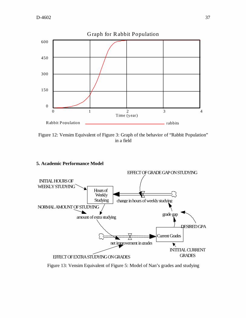
Figure 12: Vensim Equivalent of Figure 3: Graph of the behavior of “Rabbit Population” in a field

5. Academic Performance Model

EFFECT OF GRADE GAP ON STUDYING

Hours of Weekly Studying

Current Grades

change in hours of weekly studying

net improvement in grades

amount of extra studying

NORMAL AMOUNT OF STUDYING grade gap

DESIRED GPA

EFFECT OF EXTRA STUDYING ON GRADES

INITIAL HOURS OF WEEKLY STUDYING

INTITIAL CURRENT GRADES

Figure 13: Vensim Equivalent of Figure 5: Model of Nan’s grades and studying

38 D-4602

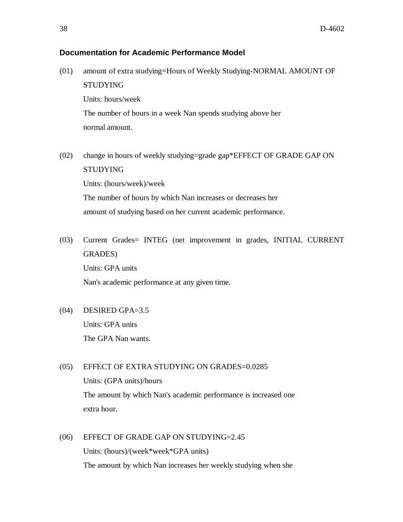
Documentation for Academic Performance Model

(01) amount of extra studying=Hours of Weekly Studying-NORMAL AMOUNT OF

STUDYING

Units: hours/week

The number of hours in a week Nan spends studying above her

normal amount.

(02) change in hours of weekly studying=grade gap*EFFECT OF GRADE GAP ON

STUDYING

Units: (hours/week)/week

The number of hours by which Nan increases or decreases her

amount of studying based on her current academic performance.

(03) Current Grades= INTEG (net improvement in grades, INITIAL CURRENT

GRADES)

Units: GPA units

Nan's academic performance at any given time.

(04) DESIRED GPA=3.5

Units: GPA units

The GPA Nan wants.

(05) EFFECT OF EXTRA STUDYING ON GRADES=0.0285

Units: (GPA units)/hours

The amount by which Nan's academic performance is increased one

extra hour.

(06) EFFECT OF GRADE GAP ON STUDYING=2.45

Units: (hours)/(week*week*GPA units)

The amount by which Nan increases her weekly studying when she

D-4602 39

is below her desired GPA by 1.0 points.

(07) FINAL TIME = 24

Units: week

The final time for the simulation.

(08) grade gap=DESIRED GPA-Current Grades

Units: GPA units

The difference between Nan's desired and actual GPA.

(09) Hours of Weekly Studying= INTEG (change in hours of weekly studying,

INITIAL HOURS OF WEEKLY STUDYING)

Units: hours/week

The number of hours Nan spends per week. The initial value of 21

hours per week corresponds corresponds to 3 hours per week.

(10) INITIAL CURRENT GRADES=3

Units: GPA units

(11) INITIAL HOURS OF WEEKLY STUDYING=21

Units: hours

(12) INITIAL TIME = 0

Units: week

The initial time for the simulation.

(13) net improvement in grades=amount of extra studying*EFFECT OF EXTRA

STUDYING ON GRADES

Units: (GPA units)/week

This is the change in Nan's grades as a result of studying more

40 D-4602

or less than her normal amount.

(14) NORMAL AMOUNT OF STUDYING=21

Units: hours/week

The number of hours Nan normally spends studying in a week.

(15) SAVEPER = TIME STEP

Units: week

The frequency with which output is stored.

(16) TIME STEP = 0.0625

Units: week

The time step for the simulation.

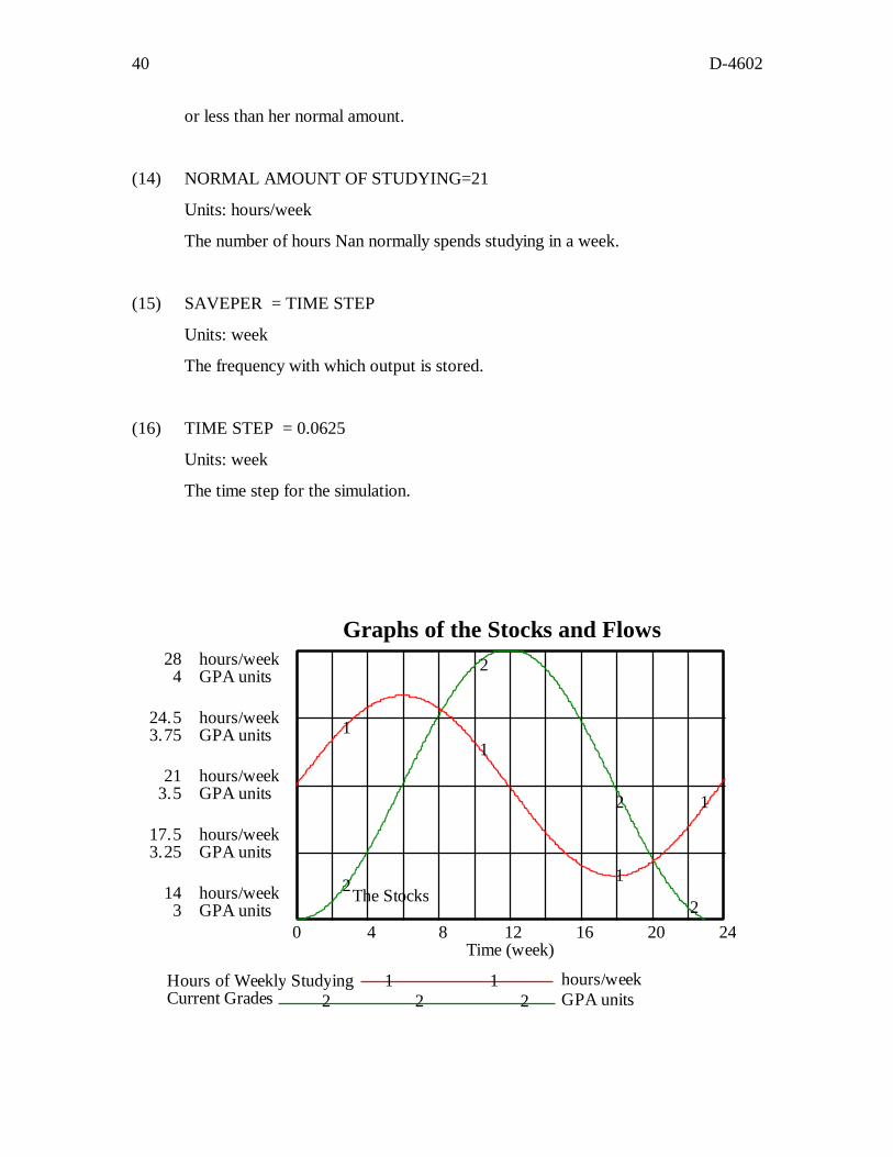
Graphs of the Stocks and Flows 28 4

hours/week GPA units

24.5 3.75

hours/week GPA units

21 hours/week 3.5 GPA units

17.5 3.25

hours/week GPA units

14 3

hours/week GPA units

0 4 8 12 16 20 24 Time (week)

Hours of Weekly Studying :Current Grades 2

1 2

1 2

hours/week GPA units

1 1

1

1

2

2

2

2The Stocks

:

D-4602 41

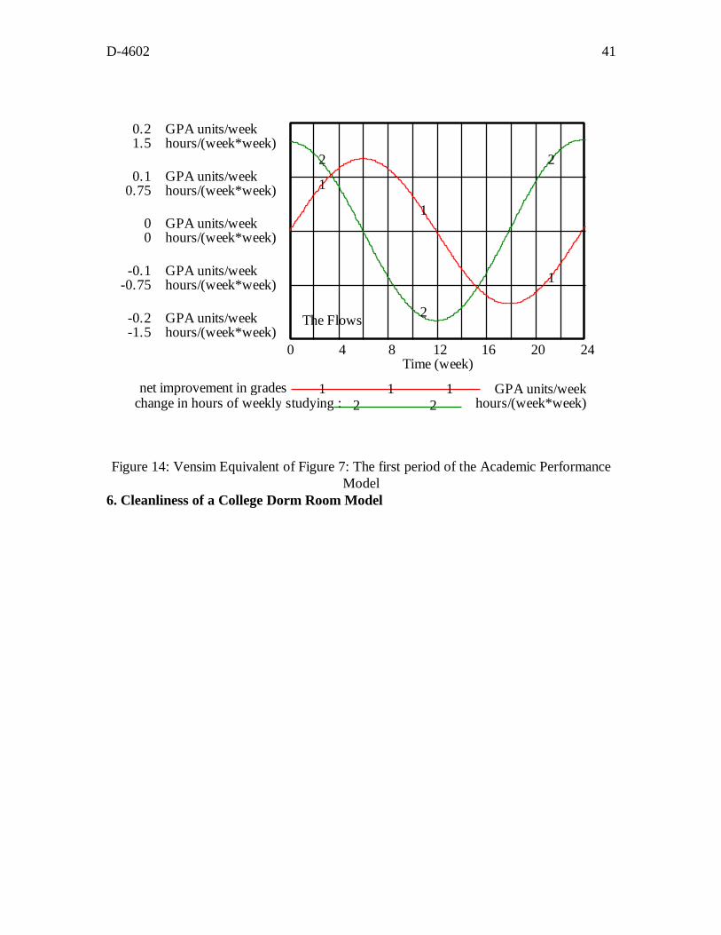
1

1

1

2

2

2

The Flows

0.2 GPA units/week 1.5 hours/(week*week)

0.1 GPA units/week 0.75 hours/(week*week)

0 GPA units/week0 hours/(week*week)

-0.1 GPA units/week-0.75 hours/(week*week)

-0.2 GPA units/week -1.5 hours/(week*week)

0 4 8 12 16 20 24 Time (week)

net improvement in grades 1 1 1 GPA units/week change in hours of weekly studying : 2 2 hours/(week*week)

Figure 14: Vensim Equivalent of Figure 7: The first period of the Academic Performance Model

6. Cleanliness of a College Dorm Room Model

42 D-4602

INITIAL LAUNDRY ON FLOOR EFFECT OF COMPLAINTS ON PICKING UP OF CLOTHES

Laundry onFloor

Daily Complaints ofMy Roommate

dropping of dirty clothes picking up of laundry

change in daily complaints of my roommate

excess laundry on floor

LAUNDRY ON FLOOR ACCEPTABLE TO ROOMMATE

EFFECT OF EXCESS LAUNDRY ON MY ROOMMATE'S COMPLAINING

INITIAL DAILY COMPLAINTS

OF MY ROOMMATE

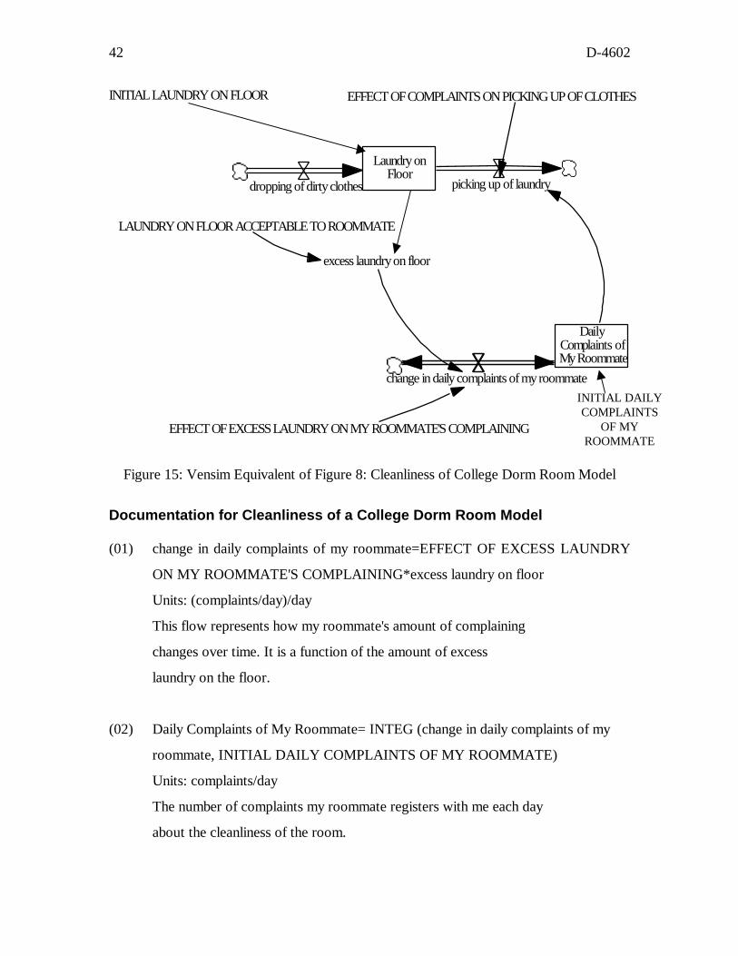
Figure 15: Vensim Equivalent of Figure 8: Cleanliness of College Dorm Room Model

Documentation for Cleanliness of a College Dorm Room Model

(01) change in daily complaints of my roommate=EFFECT OF EXCESS LAUNDRY

ON MY ROOMMATE'S COMPLAINING*excess laundry on floor

Units: (complaints/day)/day

This flow represents how my roommate's amount of complaining

changes over time. It is a function of the amount of excess

laundry on the floor.

(02) Daily Complaints of My Roommate= INTEG (change in daily complaints of my

roommate, INITIAL DAILY COMPLAINTS OF MY ROOMMATE)

Units: complaints/day

The number of complaints my roommate registers with me each day

about the cleanliness of the room.

D-4602 43

(03) dropping of dirty clothes=5

Units: clothes/day

The number of dirty clothes I drop on my floor every day. The

model assumes that my roommate's complaining does not stop me

from dropping all my clothes on the floor, it only changes how

many I pick up.

(04) EFFECT OF COMPLAINTS ON PICKING UP OF CLOTHES=1

Units: clothes/complaints

This variable is the number of extra clothes I will pick up each

day if my roommate increases his complaining by one complaint

per day.

(05) EFFECT OF EXCESS LAUNDRY ON MY ROOMMATE'S COMPLAINING=1

Units: ((complaints/day)/day)/clothes

This constant reflects how my roommate increases his complaining

based on the addition of one more article of clothing to the

floor.

(06) excess laundry on floor=Laundry on Floor-LAUNDRY ON FLOOR

ACCEPTABLE TO ROOMMATE

Units: clothes

This variable is the difference between the number of articles

of clothing on my floor and the number of articles acceptable to

my roommate.

(07) FINAL TIME = 30

Units: day

The final time for the simulation.

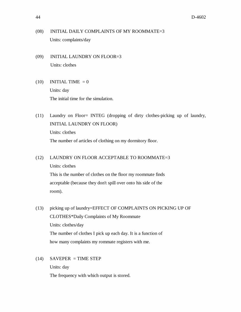
44 D-4602

(08) INITIAL DAILY COMPLAINTS OF MY ROOMMATE=3

Units: complaints/day

(09) INITIAL LAUNDRY ON FLOOR=3

Units: clothes

(10) INITIAL TIME = 0

Units: day

The initial time for the simulation.

(11) Laundry on Floor= INTEG (dropping of dirty clothes-picking up of laundry,

INITIAL LAUNDRY ON FLOOR)

Units: clothes

The number of articles of clothing on my dormitory floor.

(12) LAUNDRY ON FLOOR ACCEPTABLE TO ROOMMATE=3

Units: clothes

This is the number of clothes on the floor my roommate finds

acceptable (because they don't spill over onto his side of the

room).

(13) picking up of laundry=EFFECT OF COMPLAINTS ON PICKING UP OF

CLOTHES*Daily Complaints of My Roommate

Units: clothes/day

The number of clothes I pick up each day. It is a function of

how many complaints my rommate registers with me.

(14) SAVEPER = TIME STEP

Units: day

The frequency with which output is stored.

D-4602 45

(15) TIME STEP = 0.0625

Units: day

The time step for the simulation.

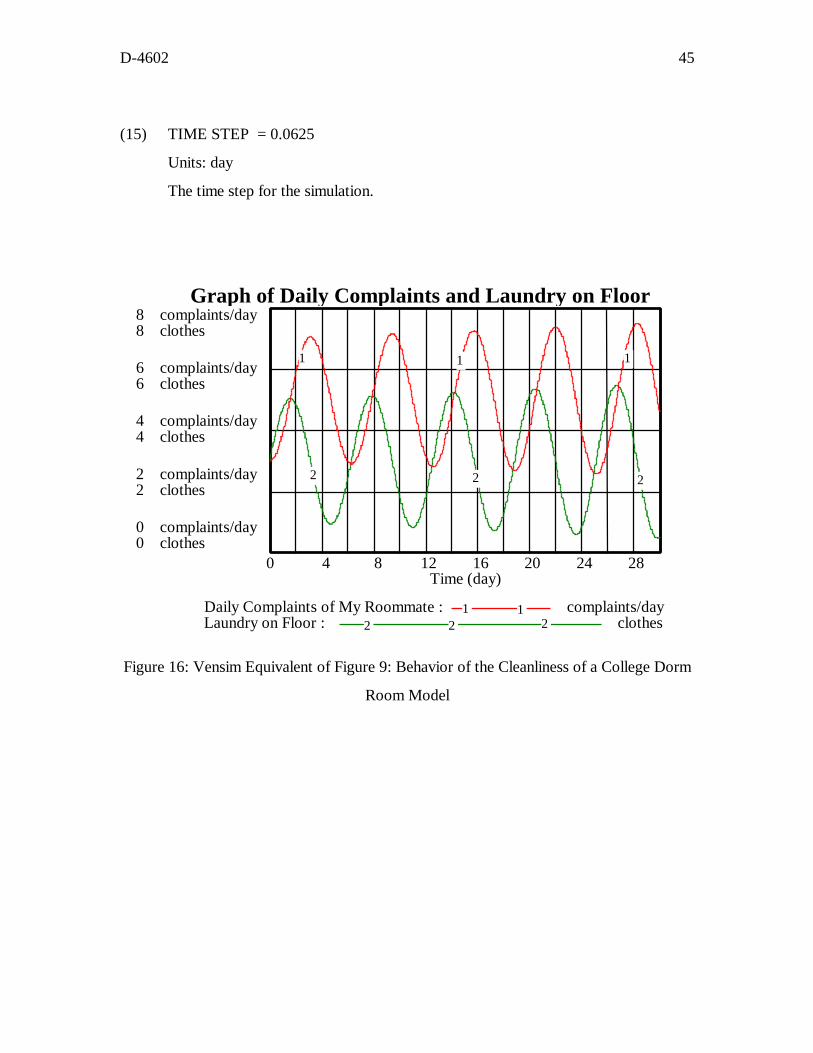
Graph of Daily Complaints and Laundry on Floor 8 complaints/day8 clothes

6 complaints/day6 clothes

4 complaints/day4 clothes

2 complaints/day2 clothes

0 complaints/day0 clothes

0 4 8 12 16 20 24 28Time (day)

Figure 16: Vensim Equivalent of Figure 9: Behavior of the Cleanliness of a College Dorm

Room Model

111

2 2 2

Daily Complaints of My Roommate : complaints/day Laundry on Floor : clothes

1 1 2 22

46

8 8

complaints/dayclothes

6 6

complaints/dayclothes

4 4

complaints/dayclothes

2 2

complaints/dayclothes

0 0

complaints/dayclothes

D-4602

2 2

2

1

1

1

The Stocks

0 2 4 6 8 10 12 Time (day)

Daily Complaints of My Roommate : complaints/day Laundry on Floor : 2 2 2

11 clothes

2 7

complaints/(day*day) clothes/day

1 6

complaints/(day*day) clothes/day

0 5

complaints/(day*day) clothes/day

-1 4

complaints/(day*day) clothes/day

-2 3

complaints/(day*day) clothes/day

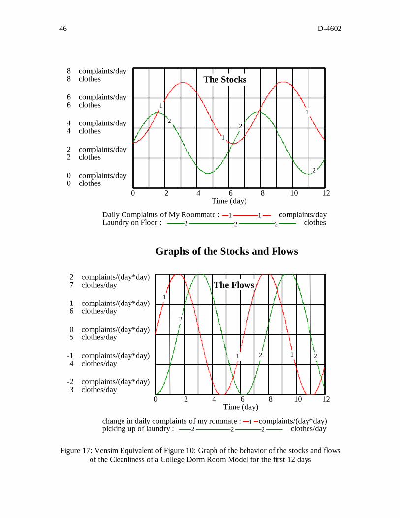
Graphs of the Stocks and Flows

1

1 1

2

22

The Flows

0 2 4 6 8 10 12 Time (day)

change in daily complaints of my rommate : 12 2

complaints/(day*day) picking up of laundry : 2 clothes/day

Figure 17: Vensim Equivalent of Figure 10: Graph of the behavior of the stocks and flows of the Cleanliness of a College Dorm Room Model for the first 12 days