INTRODUCTION TO OPERATIONS RESEARCHPresented by

Augustine Muhindo祥瑞

Mentor: Prof. Zhou Jian

34th Seminar /summer,2012

Chapter.1

1. INTRODUCTION

1.1.Origin of the operations research

• Advent of the industrial revolution

• The artisans’ small shops of an earlier era have evolved into the billion-dollar corporations of today.

• The computer revolution

1.2 THE NATURE OF OPERATIONS RESEARCH

• operations research involves “research on operations

• The process begins by carefully observing and formulating the problem, including gathering all relevant data.

• The next step is to construct a scientific (typically mathematical) model that attempts to abstract the essence of the real problem

• suitable experiments are conducted to test this hypothesis

• it attempts to resolve the conflicts of interest among the components of the organization

• OR frequently attempts to find a best

solution

1.3 THE IMPACT OF OPERATIONS RESEARCH

• improving the efficiency of numerous organizations around the world

• Has a significant contribution to increasing the productivity of the economies of various countries

CHAPTER .2

Overview of the Operations ResearchModeling Approach

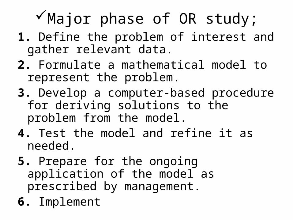
Major phase of OR study;1. Define the problem of interest and gather

relevant data.2. Formulate a mathematical model to

represent the problem.3. Develop a computer-based procedure for

deriving solutions to the problem from the model.

4. Test the model and refine it as needed.5. Prepare for the ongoing application of the

model as prescribed by management.6. Implement

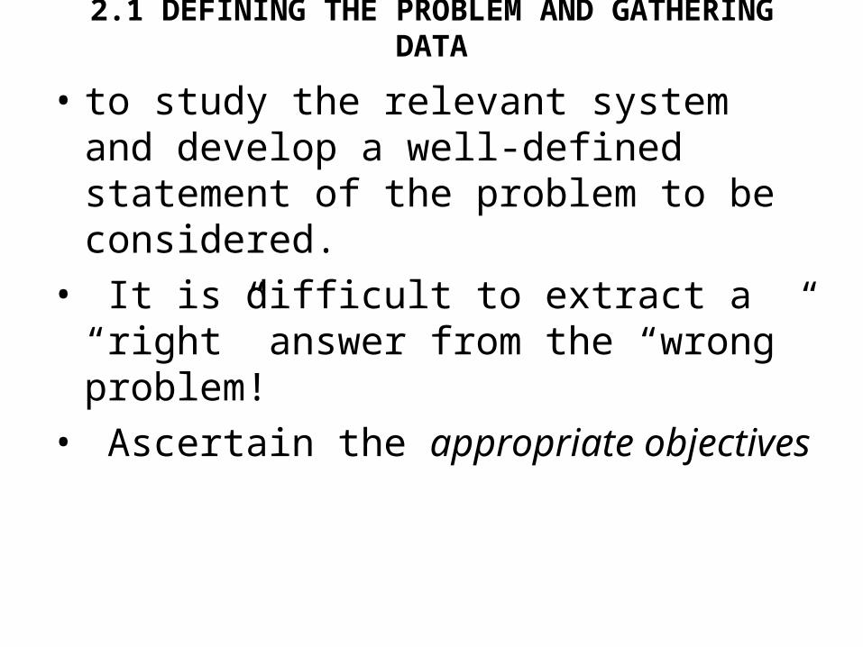
2.1 DEFINING THE PROBLEM AND GATHERING DATA

• to study the relevant system and develop a well-defined statement of the problem to be considered.

• It is difficult to extract a “right” answer from the “wrong” problem!

• Ascertain the appropriate objectives

Example!• An OR study done for the San Francisco Police

Department1 resulted in the development of a computerized system for optimally scheduling and deploying police patrol officers. The new system provided annual savings of $11 million, an annual $3 million increase in traffic citation revenues, and a 20 percent improvement in response times. In assessing the appropriate objectives for this study, three fundamental objectives were identified:

1. Maintain a high level of citizen safety.2. Maintain a high level of officer morale.3. Minimize the cost of operations

2.2 FORMULATING A MATHEMATICAL MODEL

• A mathematical model is a description of a system using mathematical concepts and language.

• The process of developing a mathematical model is termed mathematical modeling.

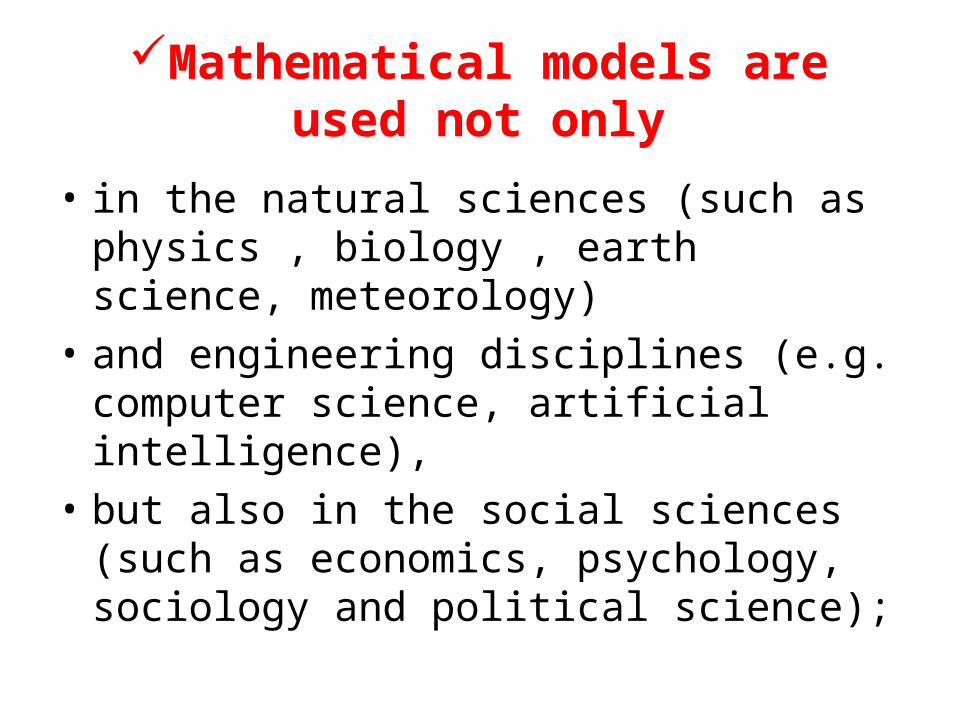
Mathematical models are used not only

• in the natural sciences (such as physics , biology , earth science, meteorology)

• and engineering disciplines (e.g. computer science, artificial intelligence),

• but also in the social sciences (such as economics, psychology, sociology and political science);

Therefore, when formulating MM, following is considered

decision variables objective function• example, x1 +3x1x2 + 2x2 < 10• Such mathematical expressions for the

restrictions often are called constraints.parameters of the model( objectives and

constraints)Sensitivity analysisLinear programming model

EXAMPLE OF MATHEMATICAL MODEL

• The potential field is given by a function V : R3 → R and the trajectory is a solution of the differential equation

• Note this model assumes the particle is a point mass, which is certainly known to be false in many cases in which we use this model; for example, as a model of planetary motion

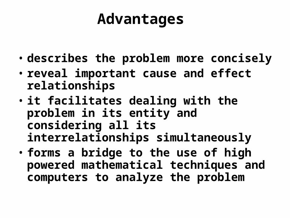
Advantages

• describes the problem more concisely• reveal important cause and effect

relationships• it facilitates dealing with the problem in its

entity and considering all its interrelationships simultaneously

• forms a bridge to the use of high powered mathematical techniques and computers to analyze the problem

Disadvantage

• Abstract idealization of the problem

2.3 DERIVING SOLUTIONS FROM THE MODEL

Heuristic procedures Post-optimality analysis • This analysis also is sometimes referred to as

what-if analysis • sensitivity analysis

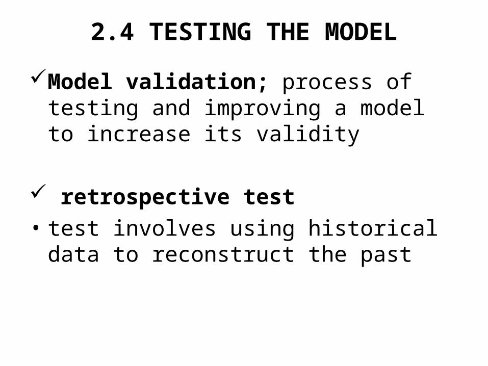
2.4 TESTING THE MODEL

Model validation; process of testing and improving a model to increase its validity

retrospective test• test involves using historical data to

reconstruct the past

2.5 PREPARING TO APPLY THE MODEL

Model procedureDecision support system; • In other cases, an interactive computer-based

system

2.6 IMPLEMENTATION

• The implementation phase involves;OR team gives operating management a

careful explanation of the new system to be adopted and how it relates to operating realities.

•

Chapter.3

Introduction to Linear Programming

Definitions of linear programmingLinear programming (LP, or linear

optimization) is a mathematical method for determining a way to achieve the best outcome (such as maximum profit or lowest cost) in a given mathematical model for some list of requirements represented as linear relationships.

More formally, linear programming is a technique for the optimization of a linear objective function, subject to linear equality and linear inequality constraints

• Its feasible region is a convex polyhedron, which is a set defined as the intersection of finitely many half spaces, each of which is defined by a linear inequality.

• Its objective function is a real-valued affine function defined on this polyhedron. A linear programming algorithm finds a point in the polyhedron where this function has the smallest (or largest) value if such point exists

• Linear programs are problems that can be expressed in canonical form

• Max cTx• Subject to: Ax ≤ b• And x≥ 0

• In fact, any problem whose mathematical model fits the very general format for the linear programming model is a linear programming problem.

• Furthermore, a remarkably efficient solution procedure, called the simplex method, is available for solving linear programming problems of even enormous size.

3.1 PROTOTYPE EXAMPLE• The WYNDOR GLASS CO. produces high-quality glass products,

including windows and glass doors. It has three plants. Aluminum frames and hardware are made in Plant 1, wood frames are made in Plant 2, and Plant 3 produces the glass and assembles the products. Because of declining earnings, top management has decided to revamp the company’s product line. Unprofitable products are being discontinued, releasing production capacity to launch two new products having large sales potential: Product 1: An 8-foot glass door with aluminum framing

• Product 2: A 4 _ 6 foot double-hung wood-framed window• Product 1 requires some of the production capacity in Plants 1 and

3, but none in Plant• 2. Product 2 needs only Plants 2 and 3. The marketing division has

concluded that the company could sell as much of either product as could be produced by these plants. However, because both products would be competing for the same production capacity in Plant 3, it is not clear which mix of the two products would be most profitable. Therefore, an OR team has been formed to study this question

TABLE 3.1 Data for the Wyndor Glass Co. problem

Production Timeper Batch, Hours

Production TimePlant 1 2 Available per Week, Hours

productsPlant 1

21 1

04

2 0 2

12

3 3 2

18

Profit per batch $3000 $5000

• Formulation as a Linear Programming Problem• • To formulate the mathematical (linear programming)

model for this problem, let• x1 = number of batches of product 1 produced per

week• x2 =number of batches of product 2 produced per

week• Z = total profit per week (in thousands of dollars) from

producing these two products• Thus, x1 and x2 are the decision variables for the

model. Using the bottom row of Table• 3.1, we obtain• Z + 3x1 +5x2.

• The objective is to choose the values of x1 and x2 so as to maximize Z =3x1 + 5x2, subject to the restrictions imposed on their values by the limited production capacities available in the three plants.

• Table 3.1 indicates that each batch of product 1 produced per week uses 1 hour of production time per week in Plant 1, whereas only 4 hours per week are available.

• This restriction is expressed mathematically by the inequality x1 ≤ 4. Similarly, Plant 2 imposes the restriction that 2x2 ≤ 12. The number of hours of production rates would be 3x1 +2x2. Therefore, the mathematical statement of the Plant 3 restriction is 3x1 +2x2 ≤18.

• Finally, since production rates cannot be negative, it is necessary to restrict the decision variables to be nonnegative: x1 ≥ 0 and x2 ≥0.

• To summarize, in the mathematical language of linear programming, the problem is

• to choose values of x1 and x2 so as to• Maximize Z = 3x1 + 5x2,• subject to the restrictions• 3x1 + 2x2 ≤ 4• 3x1 +2x2 ≤12• 3x1 + 2x2 ≤18• and• x1 ≥ 0, x2 ≥ 0.

• Graphically,

Future presentationThe linear programming modelAssumptions of linear programmingSome case studiesFormulating very large linear programming

models

• Thanks for listening.

• 你 有问题 吗？