Statistical analysis on geotechnical and geosciences data

J.P. WangDept Civil, Hong Kong University of Science and Technology (HKUST)

1

Introduction

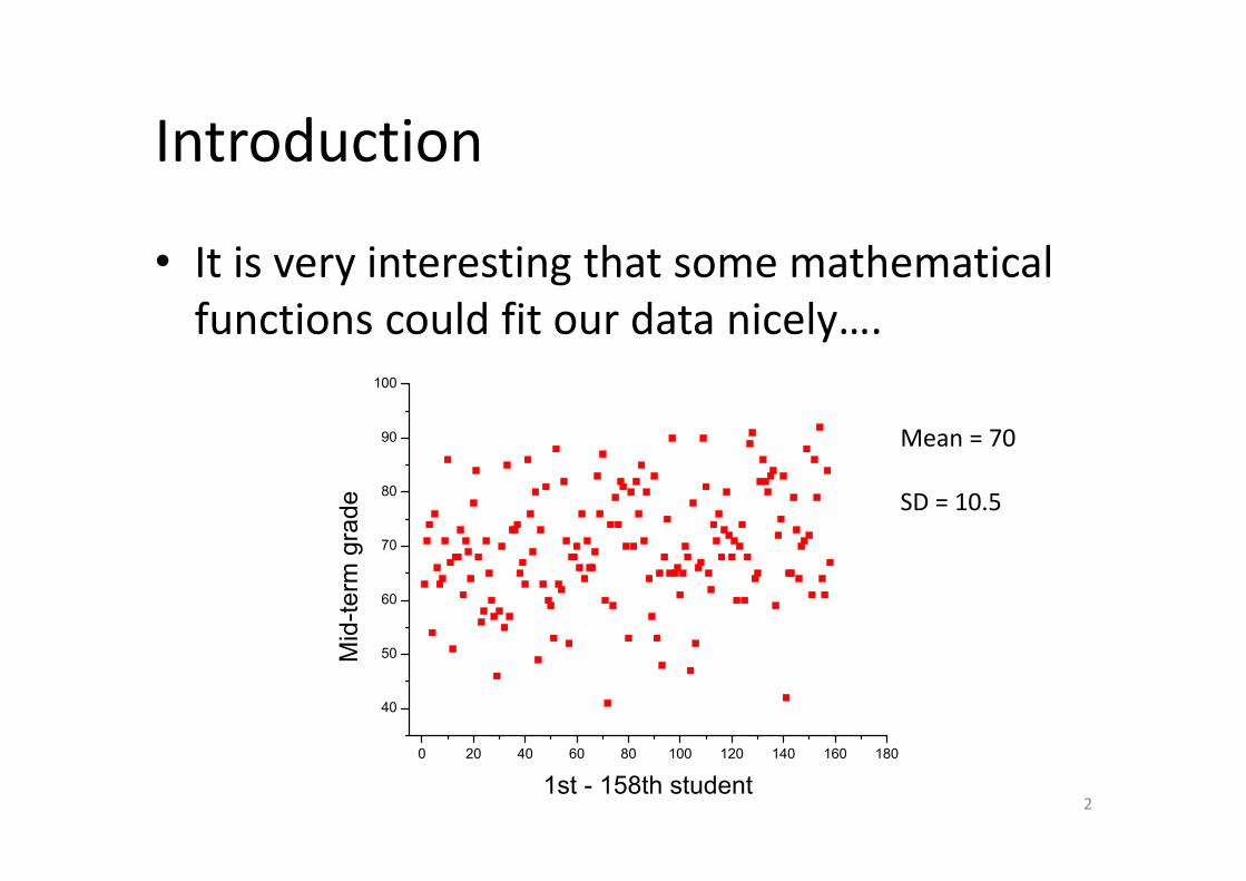
• It is very interesting that some mathematical functions could fit our data nicely….

0 20 40 60 80 100 120 140 160 180

40

50

60

70

80

90

100

Mid

-term

gra

de

1st - 158th student

Mean = 70

SD = 10.5

2

35~40 40~45 45~50 50~55 55~60 60~65 65~70 70~75 75~80 80~85 85~90 90~95 95~1000

5

10

15

20

25

30

35

Freq

uenc

y

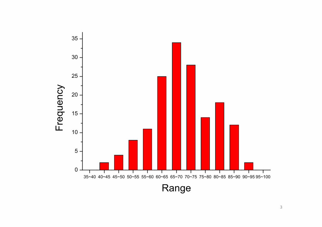
Range

3

35~40 40~45 45~50 50~55 55~60 60~65 65~70 70~75 75~80 80~85 85~90 90~95 95~1000

5

10

15

20

25

30

35

Freq

uenc

y

Range

4

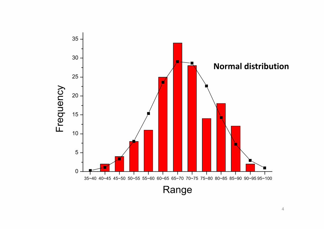
Normal distribution

• Like the “mid‐term” example, several statistical studies on earthquake and debris‐flow data will be introduced in this presentation.

• In addition to those findings, some applications will be discussed on the use of the statistical inferences from samples. 

5

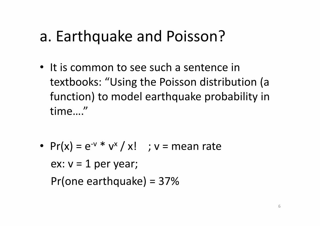
a. Earthquake and Poisson?

• It is common to see such a sentence in textbooks: “Using the Poisson distribution (a function) to model earthquake probability in time….”

• Pr(x) = e‐v * vx / x!    ; v = mean rateex: v = 1 per year; Pr(one earthquake) = 37%  

6

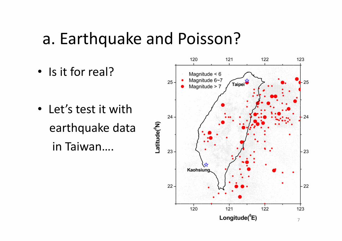
a. Earthquake and Poisson?

• Is it for real? 

• Let’s test it with earthquake data in Taiwan….

7

8

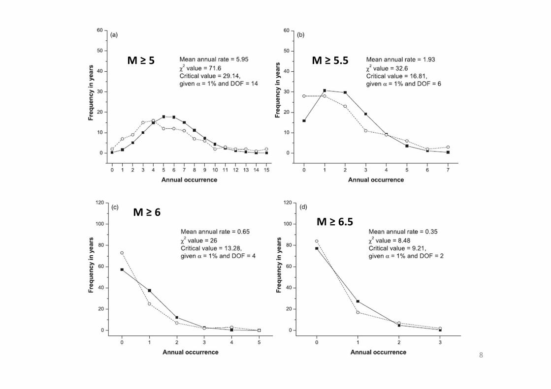
M ≥ 5 M ≥ 5.5

M ≥ 6M ≥ 6.5

• It seems that the model and observation are in good agreement.  

• Next, we changed the “boundary condition” to examine the same hypothesis.

9

10

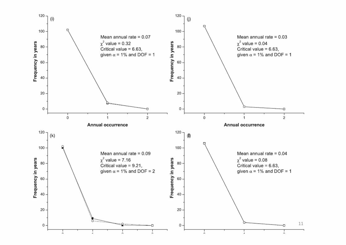
11

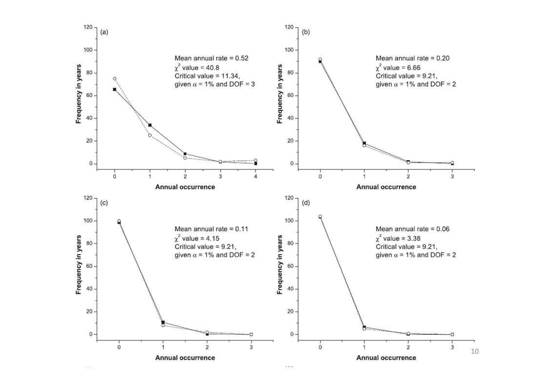
Summary (Wang et al., 2014)

• From earthquake data around Taiwan, the Poisson model and the observation are in good agreement, and the hypothesis was not rejected by Chi‐square tests, on some conditions

• A rule of thumb: mean rate = 0.1; if the mean rate < 0.1, earthquake temporal randomness could be modeled by the Poisson 

12

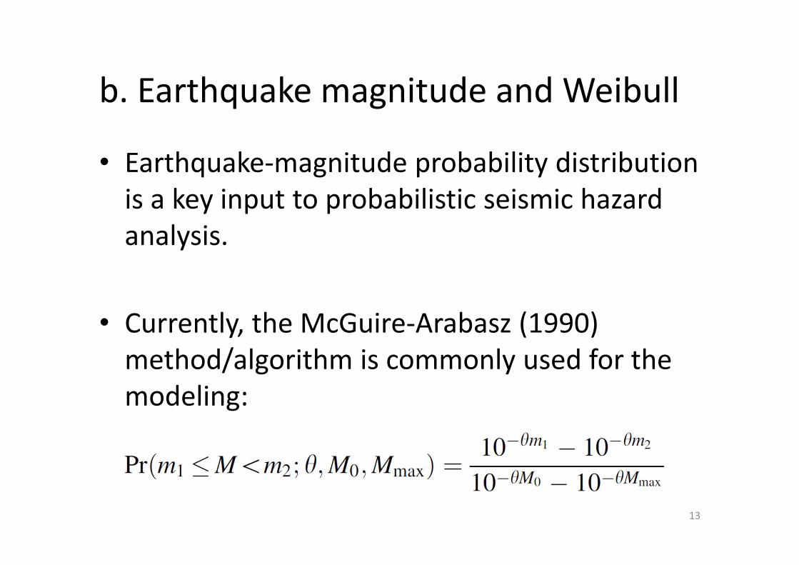
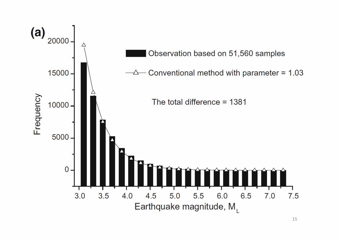
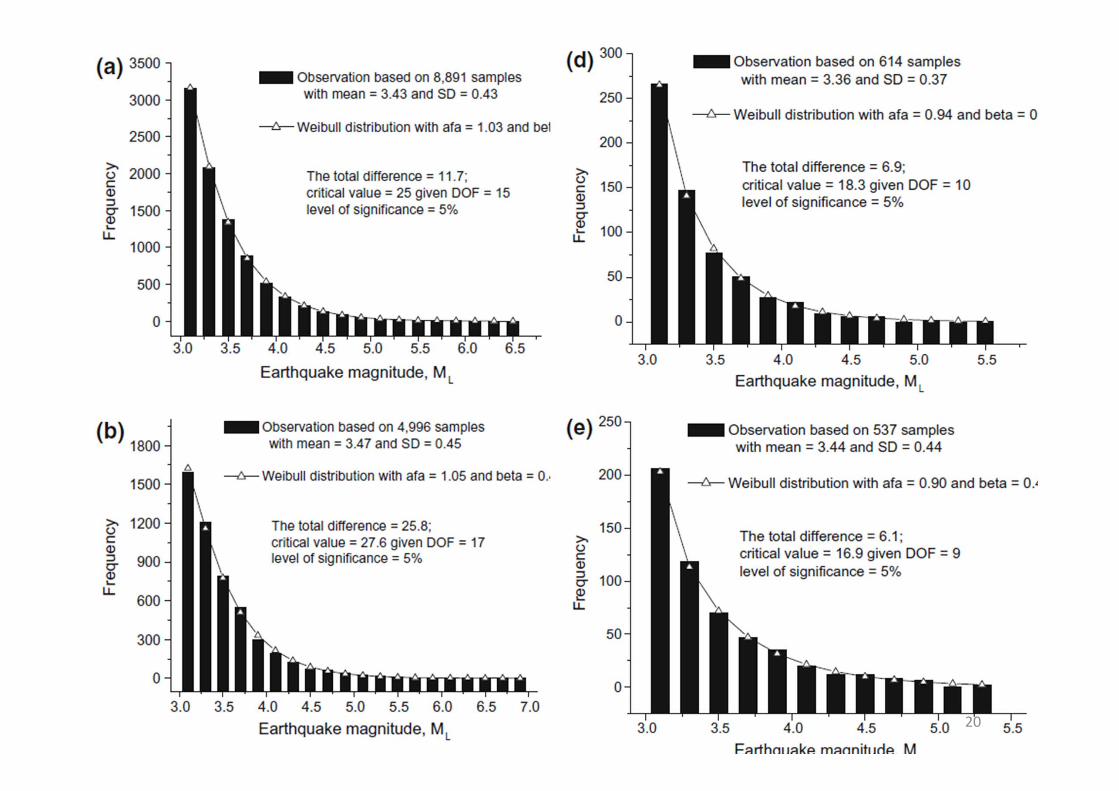
b. Earthquake magnitude and Weibull

• Earthquake‐magnitude probability distribution is a key input to probabilistic seismic hazard analysis. 

• Currently, the McGuire‐Arabasz (1990) method/algorithm is commonly used for the modeling: 

13

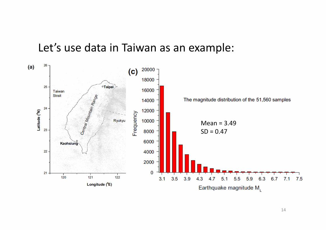
Let’s use data in Taiwan as an example:

14

Mean = 3.49SD = 0.47

15

• The Weibull distribution (a function) was discovered and proposed in the late 1930s:

• Many applications to biology, finance, and engineering (e.g., Weibull, 1939, 1951; Islam et al., 2013)

16

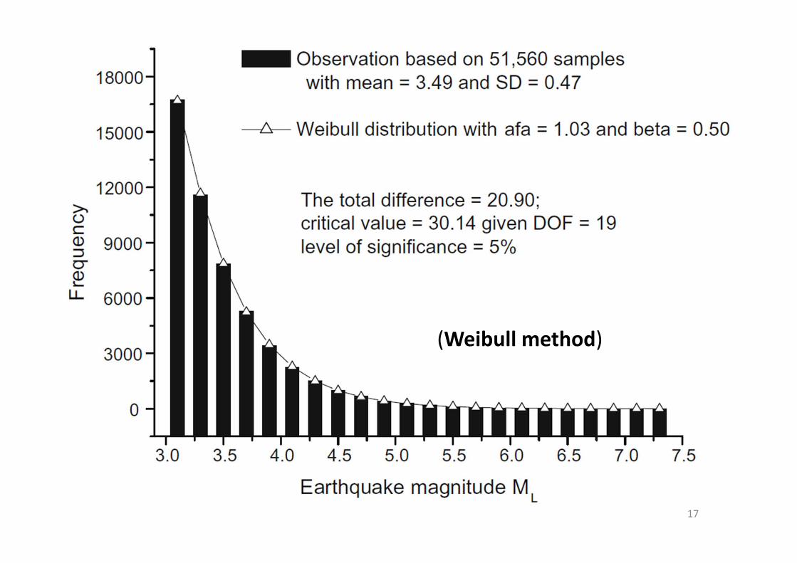
17

(Weibull method)

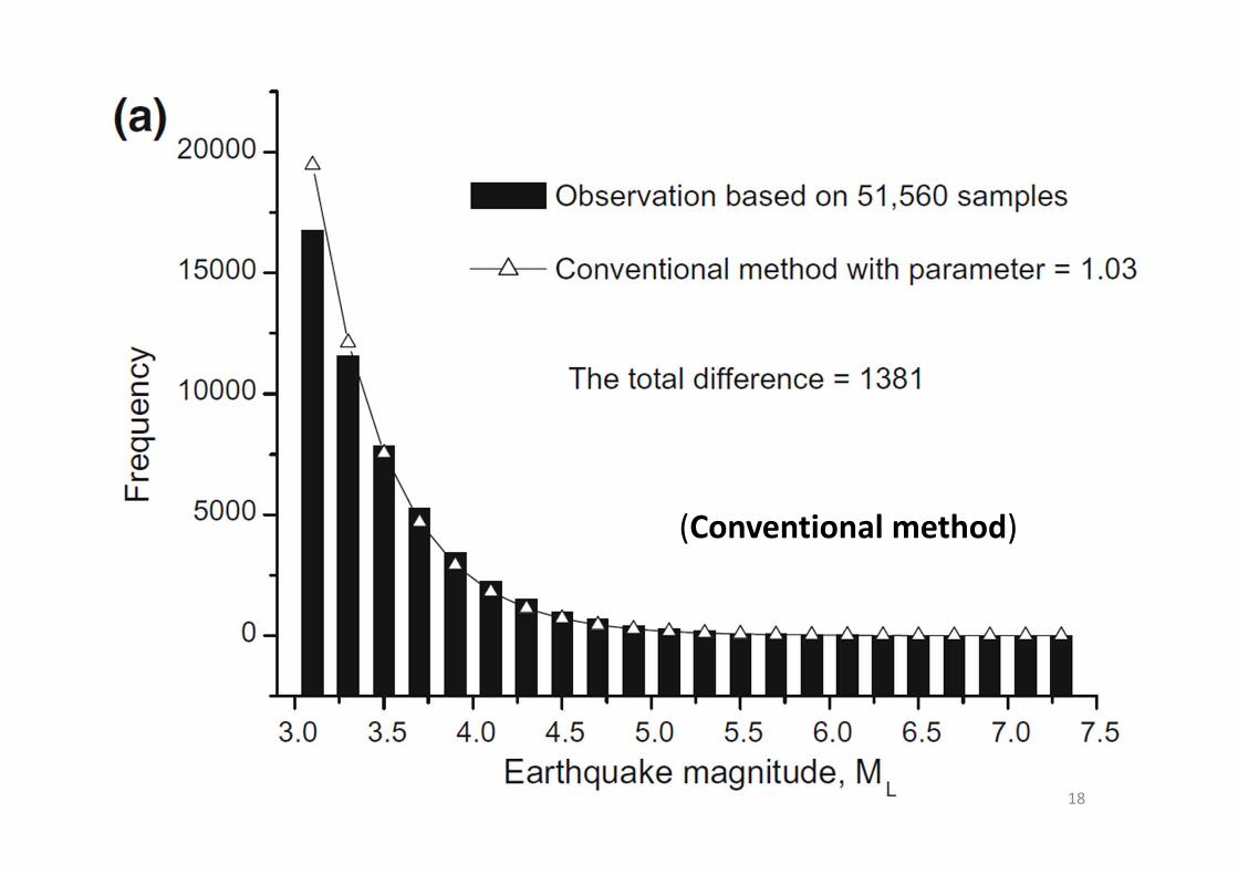
18

(Conventional method)

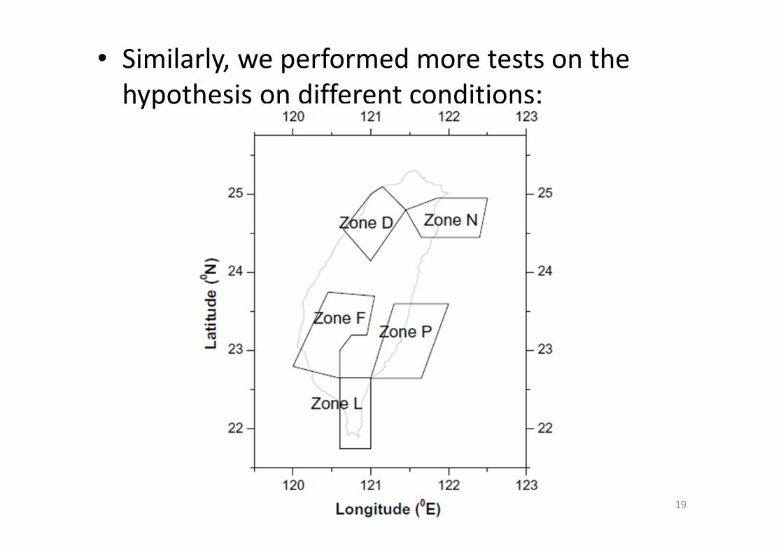
• Similarly, we performed more tests on the hypothesis on different conditions: 

19

20

Summary (Wang, 2015)

• Earthquake magnitude should be a Weibull random variable, which is supported by earthquake data around Taiwan

• The Weibull approach provides a better modeling on magnitude probability distributions, than the conventional method

21

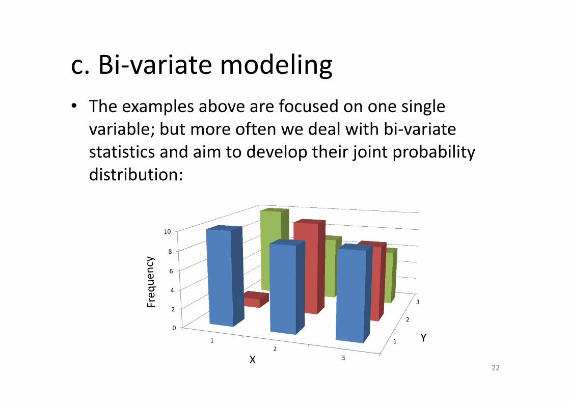
c. Bi‐variate modeling• The examples above are focused on one single variable; but more often we deal with bi‐variate statistics and aim to develop their joint probability distribution:

1

2

3

0

2

4

6

8

10

12

3X

Y

22

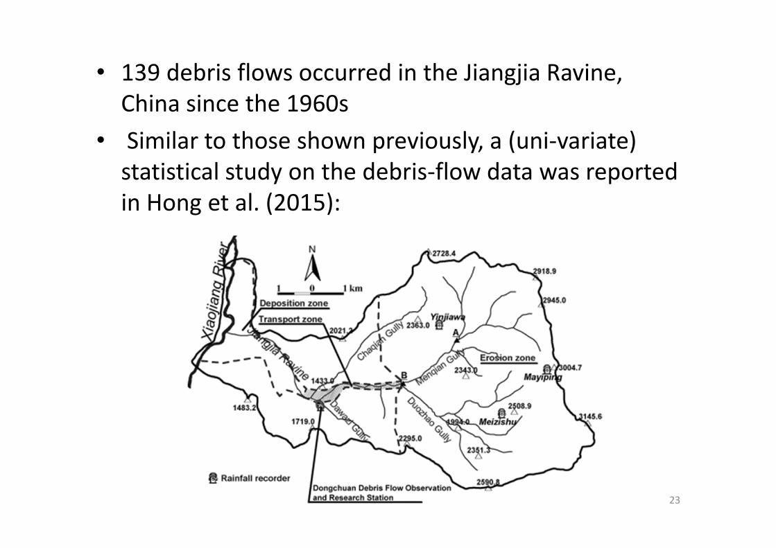
• 139 debris flows occurred in the Jiangjia Ravine, China since the 1960s

• Similar to those shown previously, a (uni‐variate) statistical study on the debris‐flow data was reported in Hong et al. (2015):

23

• The flow’s maximum impact pressure, P:

24

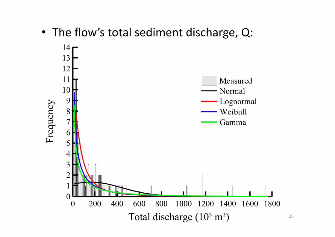
• The flow’s total sediment discharge, Q:

25

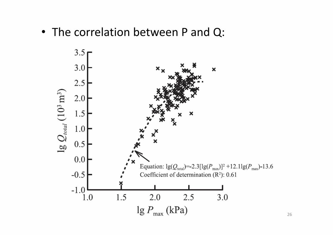
• The correlation between P and Q: 

26

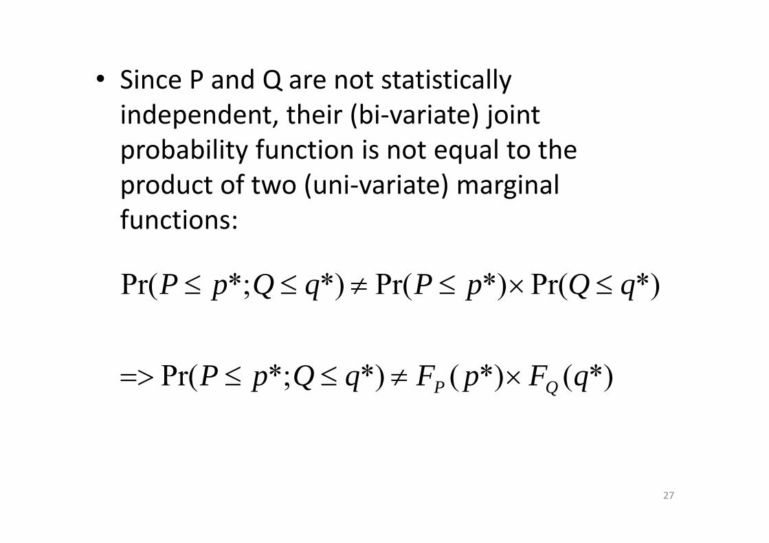
• Since P and Q are not statistically independent, their (bi‐variate) joint probability function is not equal to the product of two (uni‐variate) marginal functions:  

*)(*)(*)*;Pr(

*)Pr(*)Pr(*)*;Pr(

qFpFqQpP

qQpPqQpP

QP

27

• Therefore, in order to achieve a better modeling on the bi‐variate data, one logical approach is to adopt bi‐variate models, such as bi‐normal distribution, to fit the observation from scratch:  

28

(observation data)

• From methodology to calibration, the difficulty and effort are much increased from uni‐variate to bi‐variate statistical works....

• The copula method is increasingly applied to bi‐variate or multi‐variate modeling, for the method being more “user‐friendly”

• Li and Tang (2014) applied the copula method to model the joint probability function of soil friction angle and cohesion (the two are dependent), among many others (e.g., Goda, 2010)

29

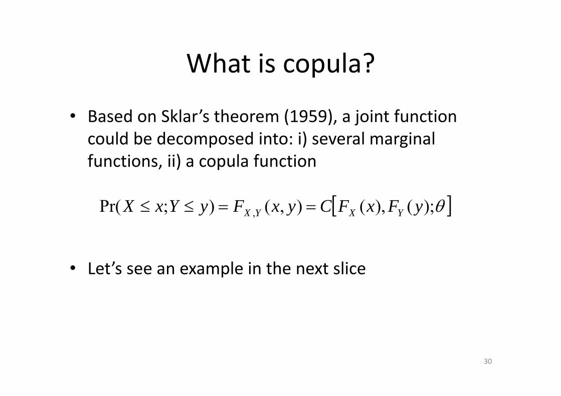
What is copula?

• Based on Sklar’s theorem (1959), a joint function could be decomposed into: i) several marginal functions, ii) a copula function

• Let’s see an example in the next slice

);(),(),();Pr( , yFxFCyxFyYxX YXYX

30

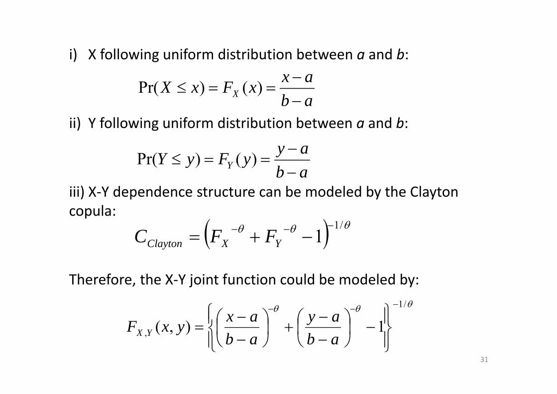
i)   X following uniform distribution between a and b:

ii)  Y following uniform distribution between a and b:

iii) X‐Y dependence structure can be modeled by the Clayton copula: 

Therefore, the X‐Y joint function could be modeled by:   

/11

YXClayton FFC

abaxxFxX X

)()Pr(

abayyFyY Y

)()Pr(

/1

, 1),(

abay

abaxyxF YX

31

• Using the copula approach, here is our best bi‐variate model for P‐Q simulation:

2.31/1.62

( ) ( )1.62 1.62249.4 237, ( , ) (1 ) (1 ) 1

p q

P QF p q e e

(Weibull + Weibull + Clayton)

Observation                                                                         Model

32

• We also applied the copula method to PGA and CAV, the two most parameters for earthquake‐resistant design

PGA

33

CAV = cumulative absolute velocity= ∫ |a| dt

• With data from Taiwan, here is our best bi‐variate model for PGA‐CAV (Xu, 2015):

(Lognormal+ Lognormal + Gaussian)

Observation                                                                         Model

34

ln * 4.44 ln * 2.84 2 2( ) ( )1 1 2 21.22 1.19

, 1 20 0

exp( 1.73 )( *, *)22.67

PGA CAV

PGA CAVr r r rF PGA CAV drdr

Summary and conclusion

• Some mathematical functions can well capture a variable’s randomness or distribution, such as using the Poisson distribution to model earthquake temporal randomness

• The copula method seems a good solution to multi‐variate statistical modeling      

35

Thank you

36