1

Introduction to Numerical Methods

2

1. Chapter 01.01 Introduction to Numerical Methods

PRE-REQUISITES (ön koşullar) 1. Be able to find integrals of a function (Primer for Integral Calculus). 2. Understand the concept of curve fitting.

OBJECTIVES (hedefler) 1. understand the need for numerical methods, and 2. go through the stages (mathematical modeling, solving and implementation) of

solving a particular physical problem. After reading this chapter, you should be able to:

1. understand the need for numerical methods, and 2. go through the stages (mathematical modeling, solving and implementation) of

solving a particular physical problem. Mathematical models are an integral (ayrılmaz/bütünü) part in solving engineering problems. Many times, these mathematical models are derived (türetilmiş) from engineering and science principles, while at other times the models may be obtained (elde edilmiş/toplanmış) from experimental data. Mathematical models generally result in need of using mathematical procedures that include but are not limited to (matematiksel modellerde matematiksel işlemlere gereksinim vardır)

(A) differentiation, (değişiklik/farklılaşma) (B) nonlinear equations, (çizgisel olmayan eşitlikler) (C) simultaneous linear equations, (aynı anda çözülen çizgisel eşitlikler) (D) curve fitting by interpolation or regression, (interpolasyon/regresyon ile eğri uydurma) (E) integration, (toplama) and (F) differential equations (diferensiyel eşitlikler).

These mathematical procedures may be suitable to be solved exactly as you must have experienced in the series of calculus courses you have taken, but in most cases, the procedures need to be solved approximately using numerical methods (derslerde matematik problemlerini analitik çözerken kesin sonuçlar elde etmişsinizdir, sayısal yöntemlerde ise yaklaşık çözümler elde edilir). Let us see an example of such a need from a real-life physical problem. To make the fulcrum (dayanak/mesnet noktası) (Figure 1) of a bascule bridge (basküllü köprü), a long hollow steel shaft (içi boş çelik şaft) called the trunnion (mafsal/dayanak) is shrink fit into a steel hub. The resulting steel trunnion-hub assembly is then shrink fit into the girder (kiriş) of the bridge.

3

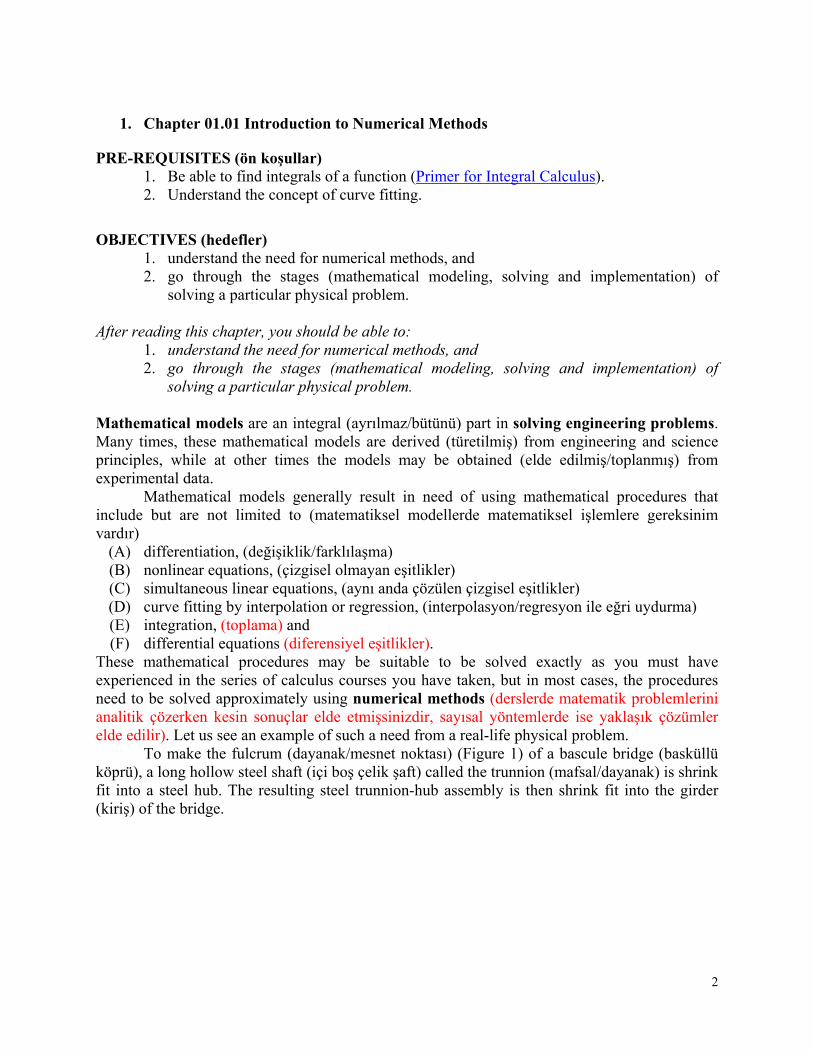
Figure 1 Trunnion-Hub-Girder (THG) assembly (mafsal-yuva-kiriş işlemi). This is done by first immersing (daldırılmış) the trunnion (mafsal) in a cold medium such as a dry-ice/alcohol mixture. After the trunnion reaches the steady state temperature of the cold medium, the trunnion outer diameter contracts. The trunnion is taken out of the medium and slid through the hole of the hub (Figure 2) (mafsal kuru buz/alkol karışımı ortamında kararlı bir sıcaklığa ulaşana kadar soğutulduktan sonra yuvasına/deliğe geçirilir. Deliğin içine tam oturması sağlanır).

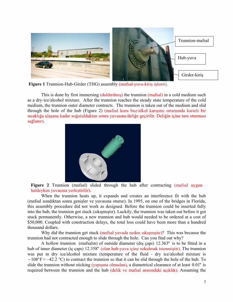
Figure 2 Trunnion (mafsal) slided through the hub after contracting (mafsal uygun haldeyken yuvasına yerleştirilir).

When the trunnion heats up, it expands and creates an interference fit with the hub (mafsal ısındıktan sonra genişler ve yuvasına oturur). In 1995, on one of the bridges in Florida, this assembly procedure did not work as designed. Before the trunnion could be inserted fully into the hub, the trunnion got stuck (sıkışmıştır). Luckily, the trunnion was taken out before it got stuck permanently. Otherwise, a new trunnion and hub would needed to be ordered at a cost of $50,000. Coupled with construction delays, the total loss could have been more than a hundred thousand dollars.

Why did the trunnion get stuck (mafsal yuvada neden sıkışmıştır)? This was because the trunnion had not contracted enough to slide through the hole. Can you find out why? A hollow trunnion (mafsalın) of outside diameter (dış çapı) "363.12 is to be fitted in a hub of inner diameter (iç çapı) "358.12 (olan hub-yuva içine sokulmak istenmiştir). The trunnion was put in dry ice/alcohol mixture (temperature of the fluid - dry ice/alcohol mixture is

F108 = –42.2 °C) to contract the trunnion so that it can be slid through the hole of the hub. To slide the trunnion without sticking (yapışma olmadan), a diametrical clearance of at least "01.0 is required between the trunnion and the hub (delik ve mafsal arasındaki açıklık). Assuming the

Trunnion-mafsal

Hub-yuva

Girder-kiriş

4

room temperature is F80 (=26.7°C), is immersing the trunnion in dry-ice/alcohol mixture a correct decision? (mafsalı kurubuz/alkol karışımına daldırmak çapını küçültmek adına doğru bir karar mıdır?) To calculate the contraction (daralma) in the diameter of the trunnion (mafsal), the thermal expansion coefficient at room temperature is used. In that case the reduction D in the outer diameter of the trunnion (mafsal) is TDD (1) where

D = outer diameter of the trunnion, coefficient of thermal expansion coefficient at room temperature, and T change in temperature,

Given D = "363.12 Fin/in/1047.6 6 at F80

T roomfluid TT = 80108 F188 ( = –122.2°C)

where

fluidT = temperature of dry-ice/alcohol mixture

roomT = room temperature

the reduction in the outer diameter of the trunnion is given by 1881047.6)363.12( 6 D = "01504.0

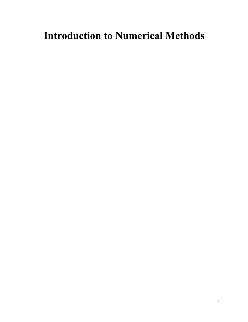
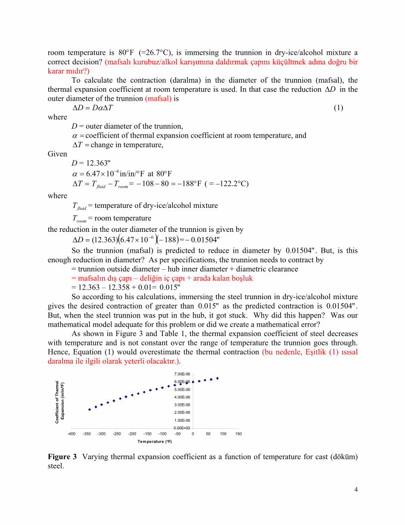
So the trunnion (mafsal) is predicted to reduce in diameter by "01504.0 . But, is this enough reduction in diameter? As per specifications, the trunnion needs to contract by = trunnion outside diameter – hub inner diameter + diametric clearance = mafsalın dış çapı – deliğin iç çapı + arada kalan boşluk = 12.363 – 12.358 + 0.01= "015.0 So according to his calculations, immersing the steel trunnion in dry-ice/alcohol mixture gives the desired contraction of greater than "015.0 as the predicted contraction is "01504.0 . But, when the steel trunnion was put in the hub, it got stuck. Why did this happen? Was our mathematical model adequate for this problem or did we create a mathematical error? As shown in Figure 3 and Table 1, the thermal expansion coefficient of steel decreases with temperature and is not constant over the range of temperature the trunnion goes through. Hence, Equation (1) would overestimate the thermal contraction (bu nedenle, Eşitlik (1) ısısal daralma ile ilgili olarak yeterli olacaktır.).

0.00E+00

1.00E-06

2.00E-06

3.00E-06

4.00E-06

5.00E-06

6.00E-06

7.00E-06

-400 -350 -300 -250 -200 -150 -100 -50 0 50 100 150

Temperature (oF)

Co

effi

cien

t o

f T

her

mal

E

xpan

cio

n (

in/in

/oF

)

Figure 3 Varying thermal expansion coefficient as a function of temperature for cast (döküm) steel.

5

The contraction (daralma) in the diameter of the trunnion (mafsal) for which the thermal expansion coefficient varies as a function of temperature is given by

fluid

room

T

T

dTDD (2)

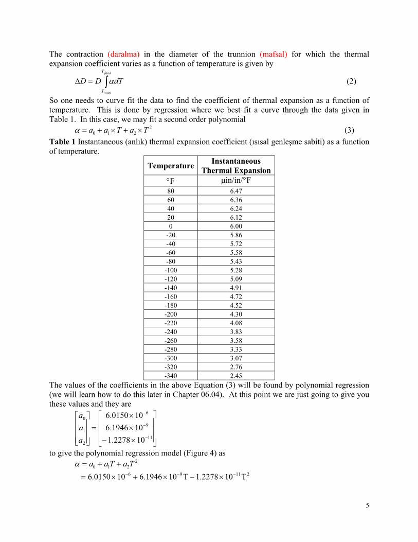
So one needs to curve fit the data to find the coefficient of thermal expansion as a function of temperature. This is done by regression where we best fit a curve through the data given in Table 1. In this case, we may fit a second order polynomial

2210 TaTaa (3)

Table 1 Instantaneous (anlık) thermal expansion coefficient (ısısal genleşme sabiti) as a function of temperature.

Temperature Instantaneous

Thermal Expansion F Fμin/in/

80 6.47 60 6.36 40 6.24 20 6.12 0 6.00

-20 5.86 -40 5.72 -60 5.58 -80 5.43 -100 5.28 -120 5.09 -140 4.91 -160 4.72 -180 4.52 -200 4.30 -220 4.08 -240 3.83 -260 3.58 -280 3.33 -300 3.07 -320 2.76 -340 2.45

The values of the coefficients in the above Equation (3) will be found by polynomial regression (we will learn how to do this later in Chapter 06.04). At this point we are just going to give you these values and they are

11

9

6

2

1

0

102278.1

101946.6

100150.6

a

a

a

to give the polynomial regression model (Figure 4) as 2

210 TaTaa

21196 T101.2278T106.1946106.0150

6

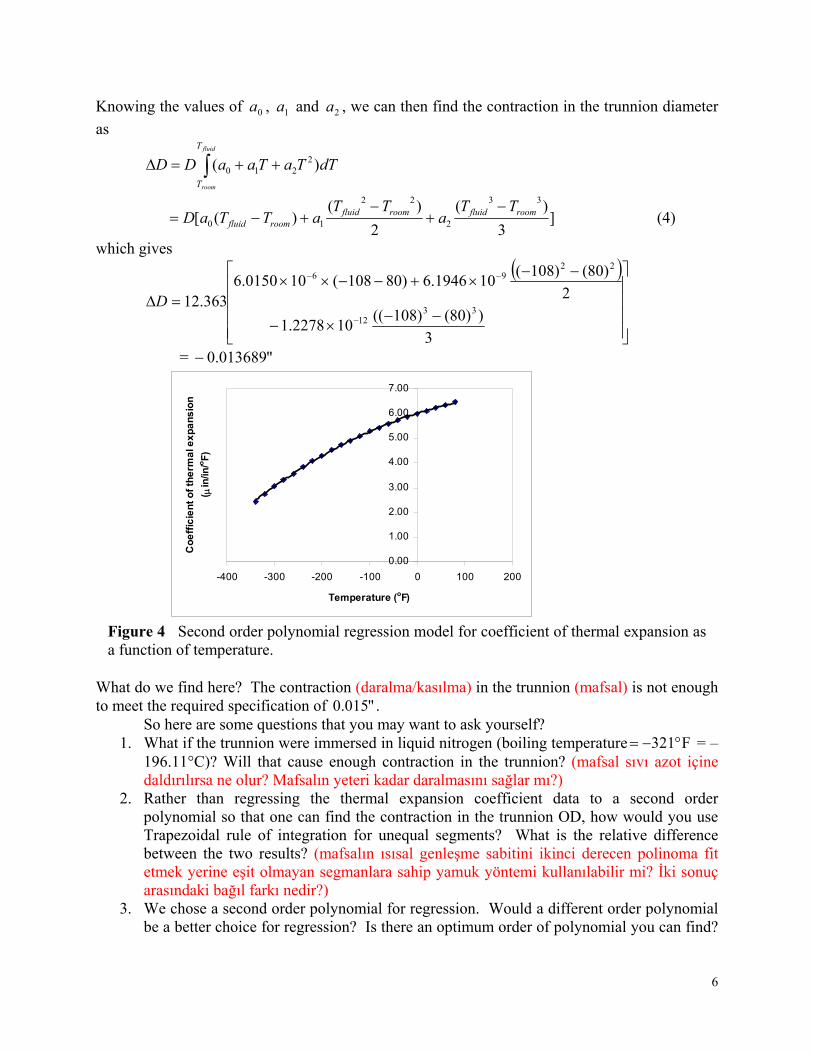
Knowing the values of 0a , 1a and 2a , we can then find the contraction in the trunnion diameter

as

dTTaTaaDDfluid

room

T

T

)( 2210

]3

)(

2

)()([

33

2

22

10roomfluidroomfluid

roomfluid

TTa

TTaTTaD

(4)

which gives

3

))80()108((102278.1

2

)80()108(101946.6)80108(100150.6

363.1233

12

2296

D

= "013689.0

0.00

1.00

2.00

3.00

4.00

5.00

6.00

7.00

-400 -300 -200 -100 0 100 200

Temperature (oF)

Co

eff

icie

nt

of

the

rma

l ex

pa

ns

ion

( in

/in/o

F)

Figure 4 Second order polynomial regression model for coefficient of thermal expansion as a function of temperature.

What do we find here? The contraction (daralma/kasılma) in the trunnion (mafsal) is not enough to meet the required specification of "015.0 . So here are some questions that you may want to ask yourself?

1. What if the trunnion were immersed in liquid nitrogen (boiling temperature F321 = –196.11°C)? Will that cause enough contraction in the trunnion? (mafsal sıvı azot içine daldırılırsa ne olur? Mafsalın yeteri kadar daralmasını sağlar mı?)

2. Rather than regressing the thermal expansion coefficient data to a second order polynomial so that one can find the contraction in the trunnion OD, how would you use Trapezoidal rule of integration for unequal segments? What is the relative difference between the two results? (mafsalın ısısal genleşme sabitini ikinci derecen polinoma fit etmek yerine eşit olmayan segmanlara sahip yamuk yöntemi kullanılabilir mi? İki sonuç arasındaki bağıl farkı nedir?)

3. We chose a second order polynomial for regression. Would a different order polynomial be a better choice for regression? Is there an optimum order of polynomial you can find?

7

(Burada ikinci dereceden polinom seçilerek regresyon yapılmıştır. Başka polinomlar seçilmesi daha iyi sonuç alabilir misiniz? En uygun polinom derecesi nedir?)

As mentioned at the beginning of this chapter, we generally see mathematical procedures that require the solution of nonlinear equations, differentiation, solution of simultaneous linear equations, interpolation, regression, integration, and differential equations. A physical example to illustrate the need for each of these mathematical procedures is given in the beginning of each chapter. You may want to look at them now to understand better why we need numerical methods in everyday life.

INTRODUCTION, APPROXIMATION AND ERRORS Topic Introduction to Numerical Methods Summary Textbook notes of Introduction to Numerical Methods Major General Engineering Authors Autar Kaw Date Aralık 8, 2016 Web Site http://numericalmethods.eng.usf.edu

1.1.1 Multiple-Choice Test Chapter 01.01 Introduction to Numerical Methods 1. Solving an engineering problem requires four steps. In order of sequence, the four steps

are (A) Formulate (formüle etmek), solve, interpret, implement (B) Solve (çözmek), formulate, interpret, implement (C) formulate, solve, implement (uygulamasını yapmak), interpret (D) formulate, implement, solve, interpret (yorum yapmak)

2. One of the roots of the equation 033 23 xxx is

(A) –1 (B) 1 (C) 3 (D) 3 3. The solution to the set of equations 2525 cba 71864 cba 15512144 cba most nearly is cba ,,

(A) (1,1,1) (B) (1,-1,1) (C) (1,1,-1) (D) does not have a unique solution.

4. The exact integral of 4

0

2cos2

xdx is most nearly

(A) –1.000 (B) 1.000 (C) 0.000 (D) 2.000

5. The value of 0.1dx

dy, given xy 3sin2 most nearly is

(A) –5.9399 (B) –1.980 (C) 0.31402 (D) 5.9918 6. The form of the exact solution of the ordinary differential equation

8

xeydx

dy 532 , 50 y is

(A) xx BeAe 5.1 (B) xx BeAe 5.1 (C) xx BeAe 5.1 (D) xx BxeAe 5.1 For a complete solution, refer to the links at the end of the book.

9

1.2 Chapter 01.02 Measuring Errors (ölçme hataları)

PRE-REQUISITES 1. Know the definition of a secant and first derivative of a function (Primer for

Differential Calculus). 2. Understand the representation of trigonometric and transcendental functions as a

Maclaurin series (Taylor Series Revisited).

OBJECTIVES 1. find the true and relative true error, 2. find the approximate and relative approximate error, 3. relate the absolute relative approximate error to the number of significant digits at

least correct in your answers, and 4. know the concept of significant digits (anlamlı haneler).

After reading this chapter, you should be able to:

1. find the true and relative true error, 2. find the approximate and relative approximate error, 3. relate the absolute relative approximate error to the number of significant digits at

least correct in your answers, and 4. know the concept of significant digits.

In any numerical analysis, errors will arise during the calculations. To be able to deal with the issue of errors, we need to

(A) identify where the error is coming from, followed by (B) quantifying the error, and lastly (C) minimize the error as per our needs.

In this chapter, we will concentrate on item (B), that is, how to quantify errors. Q: What is true error? A: True error denoted by tE is the difference between the true value (also called the exact value)

and the approximate value. True Error True value – Approximate value

Example 1 The derivative of a function )(xf at a particular value of x can be approximately calculated by

h

xfhxfxf

)()()(

of )2(f For xexf 5.07)( and 3.0h , find a) the approximate value of )2(f b) the true value of )2(f c) the true error for part (a)

Solution

10

a) h

xfhxfxf

)()()(

For 2x and 3.0h ,

3.0

)2()3.02()2(

fff

3.0

)2()3.2( ff

3.0

77 )2(5.0)3.2(5.0 ee

3.0

028.19107.22 265.10

b) The exact value of )2(f can be calculated by using our knowledge of differential calculus. xexf 5.07)(

xexf 5.05.07)(' xe 5.05.3 So the true value of )2('f is

)2(5.05.3)2(' ef 5140.9 c) True error is calculated as tE = True value – Approximate value

265.105140.9 75061.0 The magnitude of true error does not show how bad the error is. A true error of 722.0tE

may seem to be small, but if the function given in the Example 1 were ,107)( 5.06 xexf the

true error in calculating )2(f with ,3.0h would be .1075061.0 6tE This value of true

error is smaller, even when the two problems are similar in that they use the same value of the function argument, 2x and the step size, 3.0h . This brings us to the definition of relative true error. Q: What is relative true error? A: Relative true error is denoted by t and is defined as the ratio between the true error and the

true value.

Relative True Error Value True

Error True

Example 2 The derivative of a function )(xf at a particular value of x can be approximately calculated by

h

xfhxfxf

)()()('

For xexf 5.07)( and 3.0h , find the relative true error at 2x .

Solution From Example 1,

tE = True value – Approximate value

265.105140.9 75061.0

11

Relative true error is calculated as

Value True

Error Truet

5140.9

75061.0 078895.0

Relative true errors are also presented as percentages. For this example, %1000758895.0 t %58895.7

Absolute relative true errors may also need to be calculated. In such cases, |075888.0| t

= 0.0758895 = %58895.7 Q: What is approximate error? A: In the previous section, we discussed how to calculate true errors. Such errors are calculated only if true values are known. An example where this would be useful is when one is checking if a program is in working order and you know some examples where the true error is known. But mostly we will not have the luxury of knowing true values as why would you want to find the approximate values if you know the true values. So when we are solving a problem numerically, we will only have access to approximate values. We need to know how to quantify error for such cases. Approximate error is denoted by aE and is defined as the difference between the present

approximation and previous approximation. Approximate Error Present Approximation – Previous Approximation

Example 3 The derivative of a function )(xf at a particular value of x can be approximately calculated by

h

xfhxfxf

)()()('

For xexf 5.07)( and at 2x , find the following a) )2(f using 3.0h b) )2(f using 15.0h c) approximate error for the value of )2(f for part (b)

Solution a) The approximate expression for the derivative of a function is

h

xfhxfxf

)()()('

.

For 2x and 3.0h ,

3.0

)2()3.02()2('

fff

3.0

)2()3.2( ff

3.0

77 )2(5.0)3.2(5.0 ee

12

3.0

028.19107.22 265.10

b) Repeat the procedure of part (a) with ,15.0h

h

xfhxfxf

)()()(

For 2x and 15.0h ,

15.0

)2()15.02()2('

fff

15.0

)2()15.2( ff

15.0

77 )2(5.0)15.2(5.0 ee

15.0

028.1950.20 8799.9

c) So the approximate error, aE is

aE Present Approximation – Previous Approximation

265.108799.9 38474.0 The magnitude of approximate error does not show how bad the error is . An approximate error of 38300.0aE may seem to be small; but for xexf 5.06107)( , the approximate error in

calculating )2('f with 15.0h would be 61038474.0 aE . This value of approximate error

is smaller, even when the two problems are similar in that they use the same value of the function argument, 2x , and 15.0h and 3.0h . This brings us to the definition of relative approximate error. Q: What is relative approximate error? A: Relative approximate error is denoted by a and is defined as the ratio between the

approximate error and the present approximation.

Relative Approximate Error ionApproximatPresent

Error eApproximat

Example 4 The derivative of a function )(xf at a particular value of x can be approximately calculated by

h

xfhxfxf

)()()('

For xexf 5.07)( , find the relative approximate error in calculating )2(f using values from 3.0h and 15.0h .

Solution From Example 3, the approximate value of 263.10)2( f using 3.0h and

8800.9)2(' f using 15.0h .

aE Present Approximation – Previous Approximation

13

265.108799.9 38474.0 The relative approximate error is calculated as

a ionApproximatPresent

Error eApproximat

8799.9

38474.0 038942.0

Relative approximate errors are also presented as percentages. For this example, %100038942.0 a

= %8942.3 Absolute relative approximate errors may also need to be calculated. In this example

|038942.0| a 038942.0 or 3.8942%

Q: While solving a mathematical model using numerical methods, how can we use relative approximate errors to minimize the error? A: In a numerical method that uses iterative methods (yinelemeli yöntem), a user can calculate relative approximate error a at the end of each iteration. The user may pre-specify a minimum

acceptable tolerance called the pre-specified tolerance, s . If the absolute relative approximate

error a is less than or equal to the pre-specified tolerance s , that is, || a s , then the

acceptable error has been reached and no more iterations would be required. Alternatively, one may pre-specify how many significant digits they would like to be correct in their answer. In that case, if one wants at least m significant digits to be correct in the answer, then you would need to have the absolute relative approximate error, m

a 2105.0|| %.

(alternatif olarak cevabınızı anlamlı basamak/hane sayısı ile belirleyebilirsiniz. Bu durumda mutlak göreli yaklaşık hata % cinsinden m

a 2105.0|| denklemini kullanarak m istenilen

anlamlı basamak sayısı belirlenebilir.)

Example 5 If one chooses 6 terms of the Maclaurin series for xe to calculate 7.0e , how many significant digits can you trust in the solution? Find your answer without knowing or using the exact answer.

Solution

.................!2

12

x

xe x

Using 6 terms, we get the current approximation as

!5

7.0

!4

7.0

!3

7.0

!2

7.07.01

54327.0 e 0136.2

Using 5 terms, we get the previous approximation as

!4

7.0

!3

7.0

!2

7.07.01

4327.0 e 0122.2

The percentage absolute relative approximate error is

14

1000136.2

0122.20136.2

a %069527.0

Since %105.0 22a , at least 2 significant digits are correct in the answer of

0136.27.0 e Q: But what do you mean by significant digits (anlamlı basamak ile ne anlatılmak isteniyor)? A: Significant digits are important in showing the truth one has in a reported number (anlamlı basamaklar ifade edilmek istenilen sayıyı gerçek anlamında ifade edebilir). For example, if someone asked me what the population of my county is, I would respond, “The population of the Hillsborough county area is 1 million” (Örneğin birisi size yaşadığınız şehrin nüfusunu sorsa ona çok yaklaşık bir değer -1 milyon- söylersiniz). But if someone was going to give me a $100 for every citizen of the county, I would have to get an exact count (her yurttaş için 100$ verileceği söylense bu durumda kesin rakam -2003 yılı için 1,079,587 kişi şeklinde- belirtmek durumunda kalırsınız). That count would have been 1,079,587 in year 2003. So you can see that in my statement that the population is 1 million, that there is only one significant digit, that is, 1, and in the statement that the population is 1,079,587, there are seven significant digits (1 milyon şeklinde söylediğinizde 1 anlamlı basamağı olan nüfus sayısı 1,079,587 rakamında 7 anlamlı nüfus sayısı ile ifade edilir). So, how do we differentiate the number of digits correct in 1,000,000 and 1,079,587? Well for that, one may use scientific notation. For our data we show

6

6

10079587.1587,079,1

101000,000,1

to signify the correct number of significant digits.

Example 5 Give some examples of showing the number of significant digits.

Solution (a) 0.0459 has three significant digits (b) 4.590 has four significant digits (c) 4008 has four significant digits (d) 4008.0 has five significant digits (e) 310079.1 has four significant digits (f) 3100790.1 has five significant digits (g) 31007900.1 has six significant digits

INTRODUCTION, APPROXIMATION AND ERRORS Topic Measuring Errors Summary Textbook notes on measuring errors Major General Engineering Authors Autar Kaw Date Aralık 8, 2016 Web Site http://numericalmethods.eng.usf.edu

15

1.2.1 Multiple-Choice Test Chapter 01.02 Measuring Errors 1. True error is defined as

(A) Present Approximation – Previous Approximation (B) True Value – Approximate Value (C) abs (True Value – Approximate Value) (D) abs (Present Approximation – Previous Approximation)

2. The expression for true error in calculating the derivative of x2sin at 4/x by using

the approximate expression

h

xfhxfxf

is

(A) h

hh 12cos (B)

h

hh 1cos (C)

h

h2cos1 (D)

h

h2sin

3. The relative approximate error at the end of an iteration to find the root of an equation is

%004.0 . The least number of significant digits we can trust in the solution is (A) 2 (B) 3 (C) 4 (D) 5

4. The number 31001850.0 has ________ significant digits

(A) 3 (B) 4 (C) 5 (D) 6

5. The following gas stations were cited for irregular dispensation by the Department of Agriculture. Which one cheated you the most?

Station Actual gasoline dispensed Gasoline reading at pump Ser Cit Hus She

9.90 19.90 29.80 29.95

10.00 20.00 30.00 30.00

(A) Ser (B) Cit (C) Hus (D) She 6. The number of significant digits in the number 219900 is

(A) 4 (B) 5 (C) 6 (D) 4 or 5 or 6 For a complete solution, refer to the links at the end of the book.

16

1.3 Chapter 01.03 Sources of Error

PRE-REQUISITES 1. Binary representation of numbers (Binary representation of numbers) 2. Know the definition of a secant and first derivative of a function (Primer for

Differential Calculus). 3. Know the Riemann sum concept of integration (Primer for Integral Calculus). 4. Understand the representation of trigonometric and transcendental functions as a

Maclaurin series (Taylor Series Revisited).

OBJECTIVES 1. know that there are two inherent (tabiatından) sources of error in numerical methods

– round-off (yuvarlama hatası) and truncation error (kesme hatası), 2. recognize the sources of round-off and truncation error, and 3. know the difference between round-off and truncation error.

After reading this chapter, you should be able to:

1. know that there are two inherent sources of error in numerical methods – round-off and truncation error,

2. recognize the sources of round-off and truncation error, and 3. know the difference between round-off and truncation error.

Error in solving an engineering or science problem can arise due to several factors. First, the error may be in the modeling technique. A mathematical model may be based on using assumptions that are not acceptable. For example, one may assume that the drag force on a car is proportional to the velocity of the car, but actually it is proportional to the square of the velocity of the car. This itself can create huge errors in determining the performance of the car, no matter how accurate the numerical methods you may use are. Second, errors may arise from mistakes in programs themselves or in the measurement of physical quantities. But, in applications of numerical methods itself, the two errors we need to focus on are

1. Round off error 2. Truncation error.

Q: What is round off error?

A: A computer can only represent a number approximately. For example, a number like 3

1 may

be represented as 0.333333 on a PC. Then the round off error in this case is

30000003.0333333.03

1 . Then there are other numbers that cannot be represented exactly.

For example, and 2 are numbers that need to be approximated in computer calculations. Q: What problems can be created by round off errors? A: Twenty-eight Americans were killed on February 25, 1991. An Iraqi Scud hit the Army barracks in Dhahran, Saudi Arabia. The patriot defense system had failed to track and intercept the Scud. What was the cause for this failure?

17

25 şubat 1991’de Irak’tan fırlatılan bir scud füzesi Suudi Arabistan’ın Dahran kentindeki abd’nin askeri kışlasına düşmüş, 28 amerikalı asker ölmüş ve 100’nü yaralamıştır. Abd’nin Patriot savunma sistemi scud’ları izleyememiş ve scud’ları havada tahrip edememiştir. Bu hatanın aslı ne idi? The Patriot defense system consists of an electronic detection device called the range gate (erim kapısı). It calculates the area in the air space where it should look for a Scud. To find out where it should aim next, it calculates the velocity of the Scud and the last time the radar detected the Scud. Time is saved in a register that has 24 bits length. Since the internal clock of the system is measured for every one-tenth of a second, 1/10 is expressed in a 24 bit-register as 0.0001 1001 1001 1001 1001 100. However, this is not an exact representation. In fact, it would need infinite numbers of bits to represent 1/10 exactly. So, the error in the representation in decimal format is Patriot savunma sistemi menzil aralığı/kapısı denilen elektronik algılama sistemidir. Bu elektronik sistem havada bir scud’un olup olmadığını belli bir alanı tarayarak hesaplamalar yapmaktadır. Sistemin amacı scud’un hızını belirlemek ve radarda tanımlanan füzenin en son anını kayıt etmektir. O an/zaman yani saniyenin 1/10’i 24 bitlik 0.00011001100110011001100 uzunlukta bir veri olarak sisteme kayıt edilmekteydi. Sistemin kendi saatine göre bu kayıtları saniyenin 1/10 zaman aralıklarında arka arkaya tekrarlanmakta ve kayıt altına alınmaktaydı (1/10’ları toplamaktaydı). Onluk sisteme göre her kayıtta

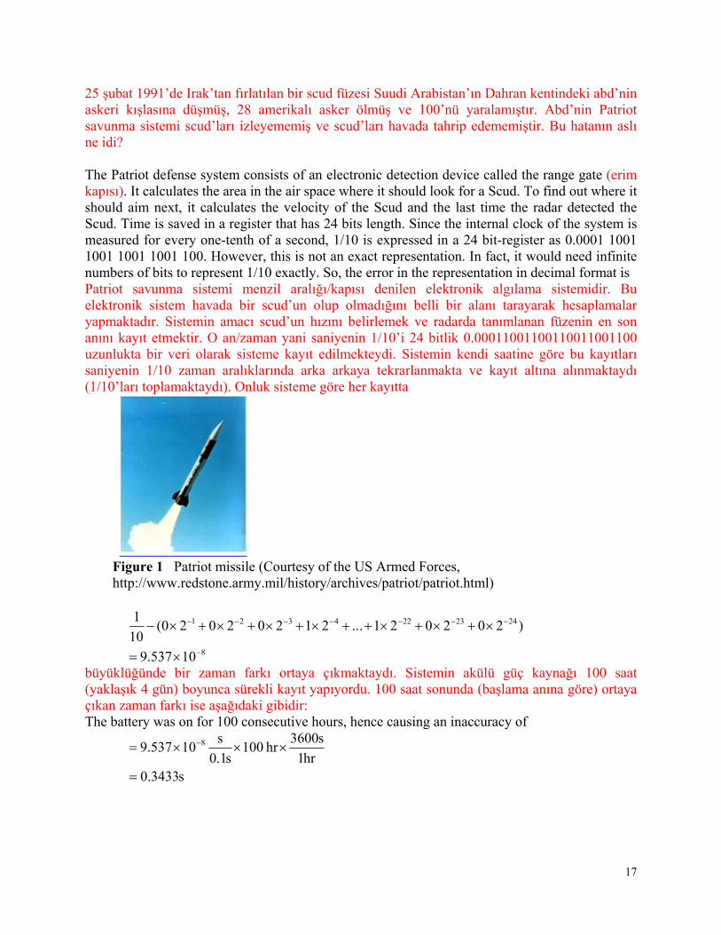
Figure 1 Patriot missile (Courtesy of the US Armed Forces, http://www.redstone.army.mil/history/archives/patriot/patriot.html)

8

2423224321

10537.9

)202021...21202020(10

1

büyüklüğünde bir zaman farkı ortaya çıkmaktaydı. Sistemin akülü güç kaynağı 100 saat (yaklaşık 4 gün) boyunca sürekli kayıt yapıyordu. 100 saat sonunda (başlama anına göre) ortaya çıkan zaman farkı ise aşağıdaki gibidir: The battery was on for 100 consecutive hours, hence causing an inaccuracy of

s3433.0hr1

s3600hr 100

s1.0

s10537.9 8

18

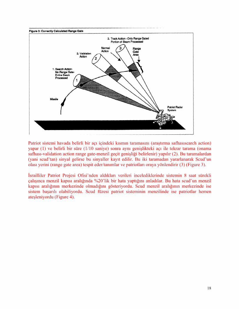
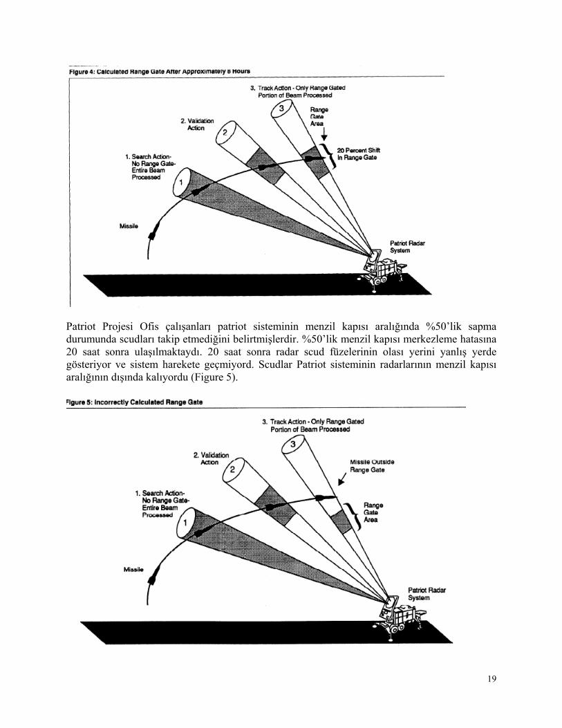
Patriot sistemi havada belirli bir açı içindeki kısmın taramasını (araştırma safhasısearch action) yapar (1) ve belirli bir süre (1/10 saniye) sonra aynı genişlikteki açı ile tekrar tarama (onama safhası-validation action range gate-menzil geçit genişliği belirlenir) yapılır (2). Bu taramalardan (yani scud’tan) sinyal gelirse bu sinyaller kayıt edilir. Bu iki taramadan yararlanarak Scud’un olası yerini (range gate area) tespit eder/tanımlar ve patriotları oraya yönlendirir (3) (Figure 3). İsrailliler Patriot Projesi Ofisi’nden aldıkları verileri incelediklerinde sistemin 8 saat sürekli çalışınca menzil kapısı aralığında %20’lik bir hata yaptığını anladılar. Bu hata scud’un menzil kapısı aralığının merkezinde olmadığını gösteriyordu. Scud menzil aralığının merkezinde ise sistem başarılı olabiliyordu. Scud füzesi patriot sisteminin menzilinde ise patriotlar hemen ateşleniyordu (Figure 4).

19

Patriot Projesi Ofis çalışanları patriot sisteminin menzil kapısı aralığında %50’lik sapma durumunda scudları takip etmediğini belirtmişlerdir. %50’lik menzil kapısı merkezleme hatasına 20 saat sonra ulaşılmaktaydı. 20 saat sonra radar scud füzelerinin olası yerini yanlış yerde gösteriyor ve sistem harekete geçmiyord. Scudlar Patriot sisteminin radarlarının menzil kapısı aralığının dışında kalıyordu (Figure 5).

20

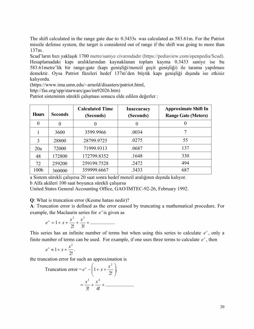
The shift calculated in the range gate due to s3433.0 was calculated as 583.61m. For the Patriot missile defense system, the target is considered out of range if the shift was going to more than

m137 . Scud’ların hızı yaklaşık 1700 metre/saniye civarındadır (https://pediaview.com/openpedia/Scud). Hesaplamadaki kapı aralıklarından kaynaklanan toplam kayma 0.3433 saniye ise bu 583.61metre’lik bir range-gate (kapı genişliği/menzil geçit genişliği) ile tarama yapılması demektir. Oysa Patriot füzeleri hedef 137m’den büyük kapı genişliği dışında ise etkisiz kalıyordu. (https://www.ima.umn.edu/~arnold/disasters/patriot.html, http://fas.org/spp/starwars/gao/im92026.htm) Patriot sisteminin sürekli çalışması sonucu elde edilen değerler :

Hours Seconds Calculated Time

(Seconds) Inaccuracy (Seconds)

Approximate Shift In Range Gate (Meters)

0 0 0 0 0

1 3600 3599.9966 .0034 7

3 28800 28799.9725 .0275 55

20a 72000 71999.9313 .0687 137

48 172800 172799.8352 .1648 330

72 259200 259199.7528 .2472 494

100b 360000 359999.6667 .3433 687

a Sistem sürekli çalışırsa 20 saat sonra hedef menzil aralığının dışında kalıyor. b Alfa aküleri 100 saat boyunca sürekli çalışırsa United States General Accounting Office, GAO/IMTEC-92-26, February 1992. Q: What is truncation error (Kesme hatası nedir)? A: Truncation error is defined as the error caused by truncating a mathematical procedure. For example, the Maclaurin series for xe is given as

....................!3!2

132

xx

xe x

This series has an infinite number of terms but when using this series to calculate xe , only a finite number of terms can be used. For example, if one uses three terms to calculate xe , then

.!2

12x

xex

the truncation error for such an approximation is

Truncation error = ,!2

12

xxe x

.......................!4!3

43

xx

21

But, how can truncation error (kesme hatası) be controlled in this example? We can use the concept (kavram) of relative approximate error to see how many terms need to be considered. Assume that one is calculating 2.1e using the Maclaurin series, then

...................!3

2.1

!2

2.12.11

322.1 e

Let us assume one wants the absolute relative approximate error to be less than 1%. In Table 1, we show the value of 2.1e , approximate error and absolute relative approximate error as a function of the number of terms, n .

n 2.1e aE %a

1 12.1 e =1 - - 2 2.112.1 e =2.2 1.2 54.546

3 !2

2.12.11

22.1 e =2.92 0.72 24.658

4 3.208 0.288 8.9776 5 3.2944 0.0864 2.6226 6 3.3151 0.020736 0.62550

Using 6 terms of the series yields a a < 1%.

Q: Can you give me other examples of truncation error? A: In many textbooks, the Maclaurin series is used as an example to illustrate truncation error. This may lead you to believe that truncation errors are just chopping a part of the series. However, truncation error can take place in other mathematical procedures as well. For example to find the derivative of a function, we define

x

xfxxfxf

x

0

lim

But since we cannot use ,0x we have to use a finite value of x , to give

x

xfxxfxf

)()()(

So the truncation error is caused by choosing a finite value of x as opposed to a .0x For example, in finding )3(f for 2)( xxf , we have the exact value calculated as follows.

2)( xxf From the definition of the derivative of a function,

x

xfxxfxf

x

)()(lim)(

0

x

xxxx

22

0

)()(lim

x

xxxxxx

222

0

)(2lim

)2(lim0

xxx

x2

22

This is the same expression you would have obtained by directly using the formula from your differential calculus class

1)( nn nxxdx

d

By this formula for 2)( xxf xxf 2)(

The exact value of )3(f is 32)3( f

6 If we now choose 2.0x , we get

2.0

)3()2.03()3(

fff

2.0

)3()2.3( ff

=2.0

32.3 22

2.0

924.10

2.0

24.1

2.6 We purposefully chose a simple function 2)( xxf with value of 2x and 2.0x because we wanted to have no round-off error in our calculations so that the truncation error can be isolated. The truncation error in this example is

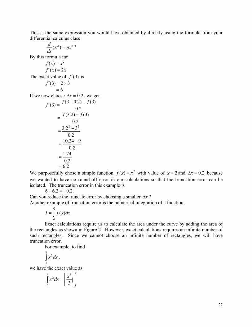
.2.02.66 Can you reduce the truncate error by choosing a smaller x ? Another example of truncation error is the numerical integration of a function,

b

a

dxxfI )(

Exact calculations require us to calculate the area under the curve by adding the area of the rectangles as shown in Figure 2. However, exact calculations requires an infinite number of such rectangles. Since we cannot choose an infinite number of rectangles, we will have truncation error. For example, to find

dxx9

3

2 ,

we have the exact value as

9

3

2dxx9

3

3

3

x

23

3

39 33

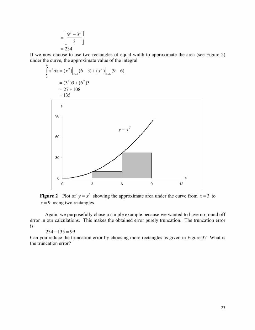
234 If we now choose to use two rectangles of equal width to approximate the area (see Figure 2) under the curve, the approximate value of the integral

)69()()36()(6

2

3

29

3

2 xx

xxdxx

3)6(3)3( 22 10827 135

y = x2

0

30

60

90

0 3 6 9 12

y

x

Figure 2 Plot of 2xy showing the approximate area under the curve from 3x to

9x using two rectangles. Again, we purposefully chose a simple example because we wanted to have no round off error in our calculations. This makes the obtained error purely truncation. The truncation error is

99135234 Can you reduce the truncation error by choosing more rectangles as given in Figure 3? What is the truncation error?

24

y = x2

0

30

60

90

0 1.5 3 4.5 6 7.5 9 10.5 12

y

x

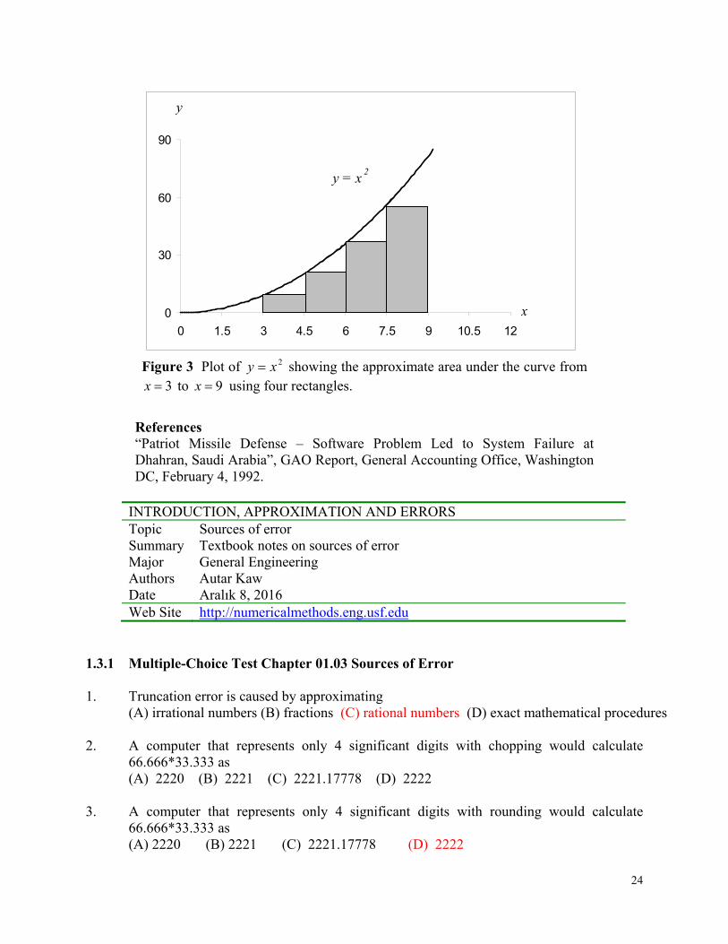
Figure 3 Plot of 2xy showing the approximate area under the curve from

3x to 9x using four rectangles.

References “Patriot Missile Defense – Software Problem Led to System Failure at Dhahran, Saudi Arabia”, GAO Report, General Accounting Office, Washington DC, February 4, 1992.

INTRODUCTION, APPROXIMATION AND ERRORS Topic Sources of error Summary Textbook notes on sources of error Major General Engineering Authors Autar Kaw Date Aralık 8, 2016 Web Site http://numericalmethods.eng.usf.edu

1.3.1 Multiple-Choice Test Chapter 01.03 Sources of Error 1. Truncation error is caused by approximating

(A) irrational numbers (B) fractions (C) rational numbers (D) exact mathematical procedures 2. A computer that represents only 4 significant digits with chopping would calculate

66.666*33.333 as (A) 2220 (B) 2221 (C) 2221.17778 (D) 2222

3. A computer that represents only 4 significant digits with rounding would calculate

66.666*33.333 as (A) 2220 (B) 2221 (C) 2221.17778 (D) 2222

25

4. The truncation error in calculating 2f for 2xxf by

h

xfhxfxf

with 2.0h is (A) –0.2 (B) 0.2 (C) 4.0 (D) 4.2

5. The truncation error in finding

9

3

3dxx using LRAM (left end point Riemann

approximation) with equally portioned points 96303 is (A) 648 (B) 756 (C) 972 (D) 1620

6. The number 1/10 is registered in a fixed 6 bit-register with all bits used for the fractional

part. The difference gets accumulated every 1/10th of a second for one day. The magnitude of the accumulated difference is (A) 0.082 (B) 135 (C) 270 (D) 5400

For a complete solution, refer to the links at the end of the book.

26

1.4 Chapter 01.04 Binary Representation

PRE-REQUISITES 1. Long Division

OBJECTIVES 1. convert a base-10 real number to its binary representation, 2. convert a binary number to an equivalent base-10 number.

After reading this chapter, you should be able to:

3. convert a base-10 real number to its binary representation, 4. convert a binary number to an equivalent base-10 number.

In everyday life, we use a number system with a base of 10. For example, look at the number 257.56. Each digit in 257.56 has a value of 0 through 9 and has a place value. It can be written as

21012 10610710710510276.257 In a binary system, we have a similar system where the base is made of only two digits 0 and 1. So it is a base 2 system. A number like (1011.0011) in base-2 represents the decimal number as

1875.11

)21212020()21212021()0011.1011( 1043210123

2

in the decimal system. To understand the binary system, we need to be able to convert binary numbers to decimal numbers and vice-versa. We have already seen an example of how binary numbers are converted to decimal numbers. Let us see how we can convert a decimal number to a binary number. For example take the decimal number 11.1875. First, look at the integer part: 11.

1. Divide 11 by 2. This gives a quotient of 5 and a remainder of 1. Since the remainder is 1, 10 a .

2. Divide the quotient 5 by 2. This gives a quotient of 2 and a remainder of 1. Since the remainder is 1, 11 a .

3. Divide the quotient 2 by 2. This gives a quotient of 1 and a remainder of 0. Since the remainder is 0, 02 a .

4. Divide the quotient 1 by 2. This gives a quotient of 0 and a remainder of 1. Since the remainder is , 13 a .

Since the quotient now is 0, the process is stopped. The above steps are summarized in Table 1.

27

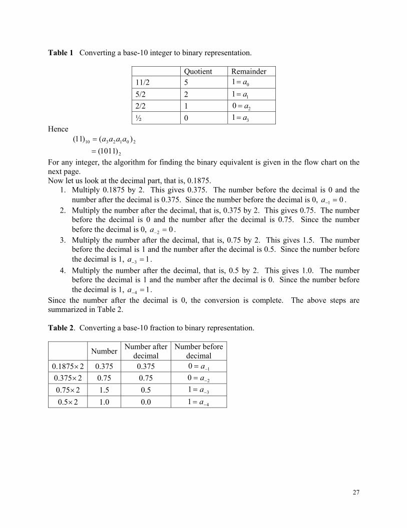
Table 1 Converting a base-10 integer to binary representation.

Quotient Remainder 11/2 5 01 a

5/2 2 11 a

2/2 1 20 a

½ 0 31 a

Hence

2

2012310

)1011(

)()11(

aaaa

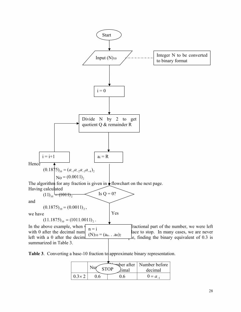
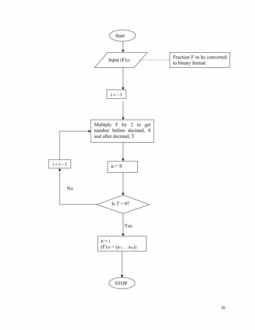
For any integer, the algorithm for finding the binary equivalent is given in the flow chart on the next page. Now let us look at the decimal part, that is, 0.1875.

1. Multiply 0.1875 by 2. This gives 0.375. The number before the decimal is 0 and the number after the decimal is 0.375. Since the number before the decimal is 0, 01 a .

2. Multiply the number after the decimal, that is, 0.375 by 2. This gives 0.75. The number before the decimal is 0 and the number after the decimal is 0.75. Since the number before the decimal is 0, 02 a .

3. Multiply the number after the decimal, that is, 0.75 by 2. This gives 1.5. The number before the decimal is 1 and the number after the decimal is 0.5. Since the number before the decimal is 1, 13 a .

4. Multiply the number after the decimal, that is, 0.5 by 2. This gives 1.0. The number before the decimal is 1 and the number after the decimal is 0. Since the number before the decimal is 1, 14 a .

Since the number after the decimal is 0, the conversion is complete. The above steps are summarized in Table 2. Table 2. Converting a base-10 fraction to binary representation.

Number Number after

decimal Number before

decimal 0.18752 0.375 0.375 10 a

0.3752 0.75 0.75 20 a

0.752 1.5 0.5 31 a

0.52 1.0 0.0 41 a

28

Hence

2

2432110

)0011.0(

)()1875.0(

aaaa

The algorithm for any fraction is given in a flowchart on the next page. Having calculated 210 )1011()11(

and 210 )0011.0()1875.0( ,

we have

210 )0011.1011()1875.11( .

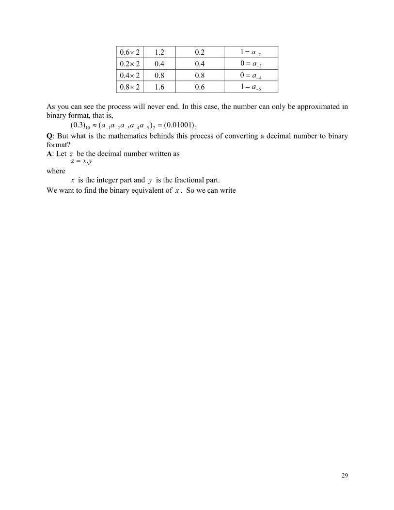
In the above example, when we were converting the fractional part of the number, we were left with 0 after the decimal number and used that as a place to stop. In many cases, we are never left with a 0 after the decimal number. For example, finding the binary equivalent of 0.3 is summarized in Table 3. Table 3. Converting a base-10 fraction to approximate binary representation.

Number Number after

decimal Number before

decimal 0.3 2 0.6 0.6 10 a

Start

Input (N)10

i = 0

Divide N by 2 to get quotient Q & remainder R

ai = R

Is Q = 0?

n = i (N)10 = (an. . .a0)2

STOP

Integer N to be converted to binary format

i = i+1

No

Yes

29

0.6 2 1.2 0.2 21 a

0.2 2 0.4 0.4 30 a

0.4 2 0.8 0.8 40 a

0.8 2 1.6 0.6 51 a

As you can see the process will never end. In this case, the number can only be approximated in binary format, that is,

225432110 )01001.0()()3.0( aaaaa

Q: But what is the mathematics behinds this process of converting a decimal number to binary format? A: Let z be the decimal number written as

yxz . where x is the integer part and y is the fractional part. We want to find the binary equivalent of x . So we can write

30

Start

Input (F)10

1i

Multiply F by 2 to get number before decimal, S and after decimal, T

ai = S

Is T = 0?

n = i (F)10 = (a-1. . .a-n)2

STOP

Fraction F to be converted to binary format

1ii

No

Yes

31

0

01

1 2...22 aaax nn

nn

If we can now find naa .,.,.0 in the above equation then

20110 )...()( aaax nn

We now want to find the binary equivalent of y . So we can write m

mbbby

2...22 2

21

1

If we can now find mbb .,.,.1 in the above equation then

22110 )...()( mbbby

Let us look at this using the same example as before.

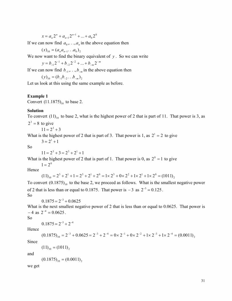
Example 1 Convert 10)1875.11( to base 2.

Solution To convert 10)11( to base 2, what is the highest power of 2 that is part of 11. That power is 3, as

823 to give 3211 3

What is the highest power of 2 that is part of 3. That power is 1, as 221 to give 123 1

So 1223211 133

What is the highest power of 2 that is part of 1. That power is 0, as 120 to give 021 Hence

2012301313

10 )1011(21212021222122)11(

To convert 10)1875.0( to the base 2, we proceed as follows. What is the smallest negative power

of 2 that is less than or equal to 0.1875. That power is 3 as 125.02 3 . So

0625.021875.0 3 What is the next smallest negative power of 2 that is less than or equal to 0.0625. That power is

4 as 0625.02 4 . So

43 221875.0 Hence

24321433

10 )0011.0(21212020220625.02)1875.0(

Since

210 )1011()11(

and

210 )0011.0()1875.0(

we get

32

210 )0011.1011()1875.11(

Can you show this algebraically for any general number?

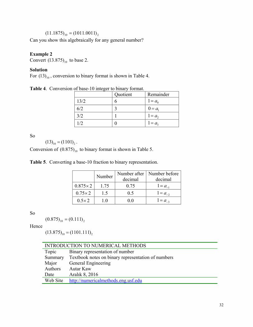
Example 2 Convert 10)875.13( to base 2.

Solution For 10)13( , conversion to binary format is shown in Table 4.

Table 4. Conversion of base-10 integer to binary format.

Quotient Remainder 13/2 6 01 a

6/2 3 10 a

3/2 1 21 a

1/2 0 31 a

So 210 )1101()13( .

Conversion of 10)875.0( to binary format is shown in Table 5.

Table 5. Converting a base-10 fraction to binary representation.

Number Number after

decimal Number before

decimal 0.8752 1.75 0.75 11 a

0.752 1.5 0.5 21 a

0.52 1.0 0.0 31 a

So 210 )111.0()875.0(

Hence

210 )111.1101()875.13(

INTRODUCTION TO NUMERICAL METHODS Topic Binary representation of number Summary Textbook notes on binary representation of numbers Major General Engineering Authors Autar Kaw Date Aralık 8, 2016 Web Site http://numericalmethods.eng.usf.edu

33

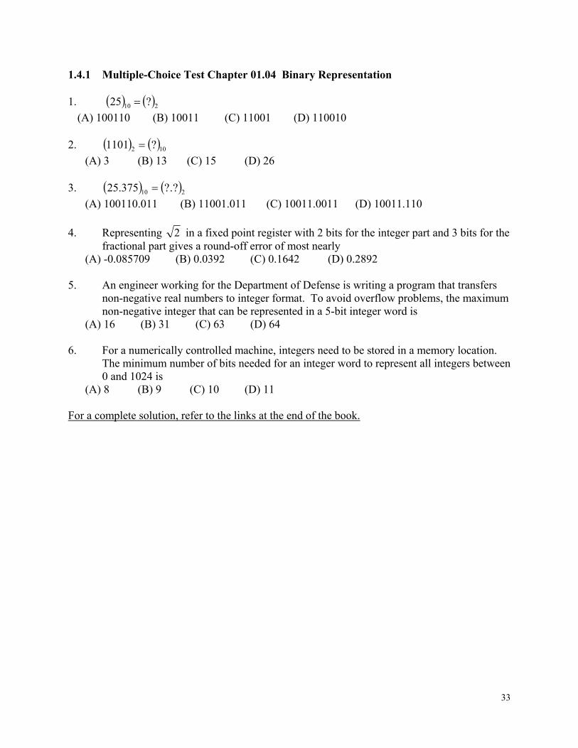
1.4.1 Multiple-Choice Test Chapter 01.04 Binary Representation 1. 210 ?25

(A) 100110 (B) 10011 (C) 11001 (D) 110010 2. 102 ?1101

(A) 3 (B) 13 (C) 15 (D) 26 3. 210 ?.?375.25

(A) 100110.011 (B) 11001.011 (C) 10011.0011 (D) 10011.110

4. Representing 2 in a fixed point register with 2 bits for the integer part and 3 bits for the fractional part gives a round-off error of most nearly

(A) -0.085709 (B) 0.0392 (C) 0.1642 (D) 0.2892 5. An engineer working for the Department of Defense is writing a program that transfers

non-negative real numbers to integer format. To avoid overflow problems, the maximum non-negative integer that can be represented in a 5-bit integer word is

(A) 16 (B) 31 (C) 63 (D) 64 6. For a numerically controlled machine, integers need to be stored in a memory location.

The minimum number of bits needed for an integer word to represent all integers between 0 and 1024 is

(A) 8 (B) 9 (C) 10 (D) 11

For a complete solution, refer to the links at the end of the book.

34

1.5 Chapter 01.05 Floating Point Representation

PRE-REQUISITES 1. Know how to represent numbers in binary format (Binary representation of numbers). 2. Know the definition of true error (Measuring Errors)

OBJECTIVES

1. convert a base-10 number to a binary floating point representation, 2. convert a binary floating point number to its equivalent base-10 number, 3. understand the IEEE-754 specifications of a floating point representation in a typical

computer, 4. calculate the machine epsilon of a representation. After reading this chapter, you should be able to:

2. convert a base-10 number to a binary floating point representation, 3. convert a binary floating point number to its equivalent base-10 number, 4. understand the IEEE-754 specifications of a floating point representation in a typical

computer, 5. calculate the machine epsilon of a representation.

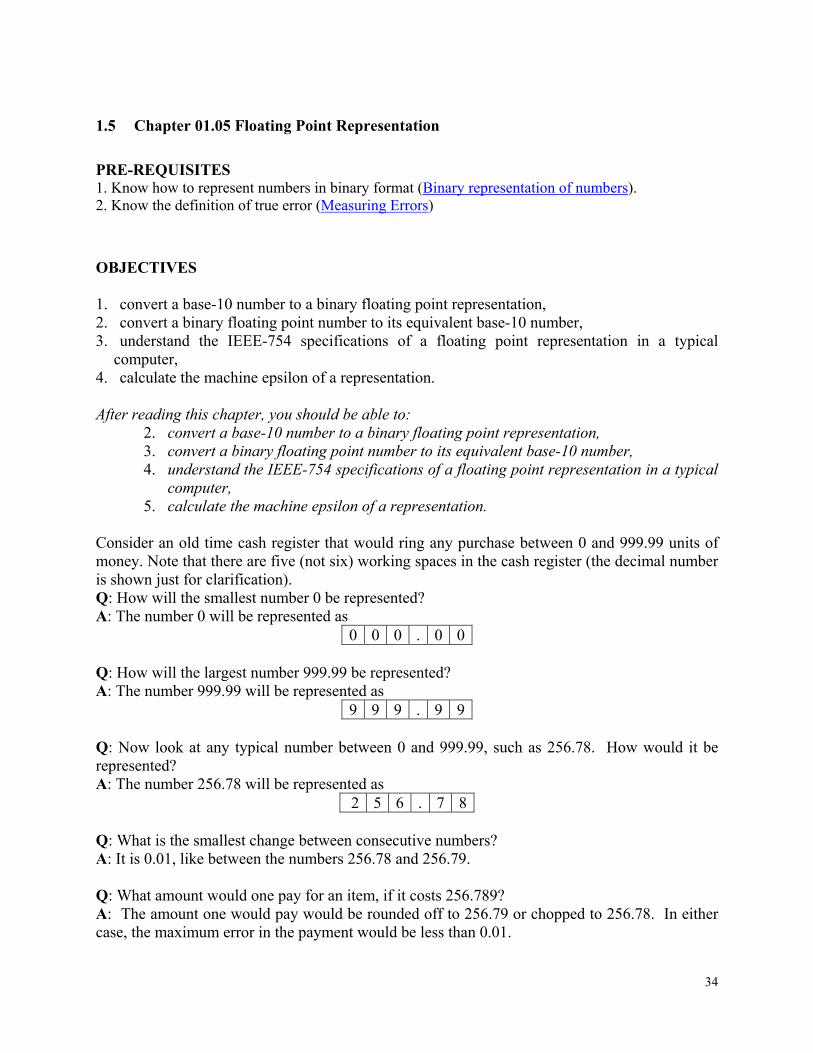
Consider an old time cash register that would ring any purchase between 0 and 999.99 units of money. Note that there are five (not six) working spaces in the cash register (the decimal number is shown just for clarification). Q: How will the smallest number 0 be represented? A: The number 0 will be represented as

0 0 0 . 0 0 Q: How will the largest number 999.99 be represented? A: The number 999.99 will be represented as

9 9 9 . 9 9 Q: Now look at any typical number between 0 and 999.99, such as 256.78. How would it be represented? A: The number 256.78 will be represented as

2 5 6 . 7 8 Q: What is the smallest change between consecutive numbers? A: It is 0.01, like between the numbers 256.78 and 256.79. Q: What amount would one pay for an item, if it costs 256.789? A: The amount one would pay would be rounded off to 256.79 or chopped to 256.78. In either case, the maximum error in the payment would be less than 0.01.

35

Q: What magnitude of relative errors would occur in a transaction? A: Relative error for representing small numbers is going to be high, while for large numbers the relative error is going to be small. For example, for 256.786, rounding it off to 256.79 accounts for a round-off error of

004.079.256786.256 . The relative error in this case is

100786.256

004.0

t %001558.0 .

For another number, 3.546, rounding it off to 3.55 accounts for the same round-off error of 004.055.3546.3 . The relative error in this case is

100546.3

004.0

t %11280.0 .

Q: If I am interested in keeping relative errors of similar magnitude for the range of numbers, what alternatives do I have? A: To keep the relative error of similar order for all numbers, one may use a floating-point representation of the number. For example, in floating-point representation, a number 256.78 is written as 2105678.2 , 0.003678 is written as ,10678.3 3 and

789.256 is written as 21056789.2 . The general representation of a number in base-10 format is given as

exponent10 mantissa sign or for a number y ,

emy 10 Where

1-or 1 number, theofsign 10 1 mantissa, mm

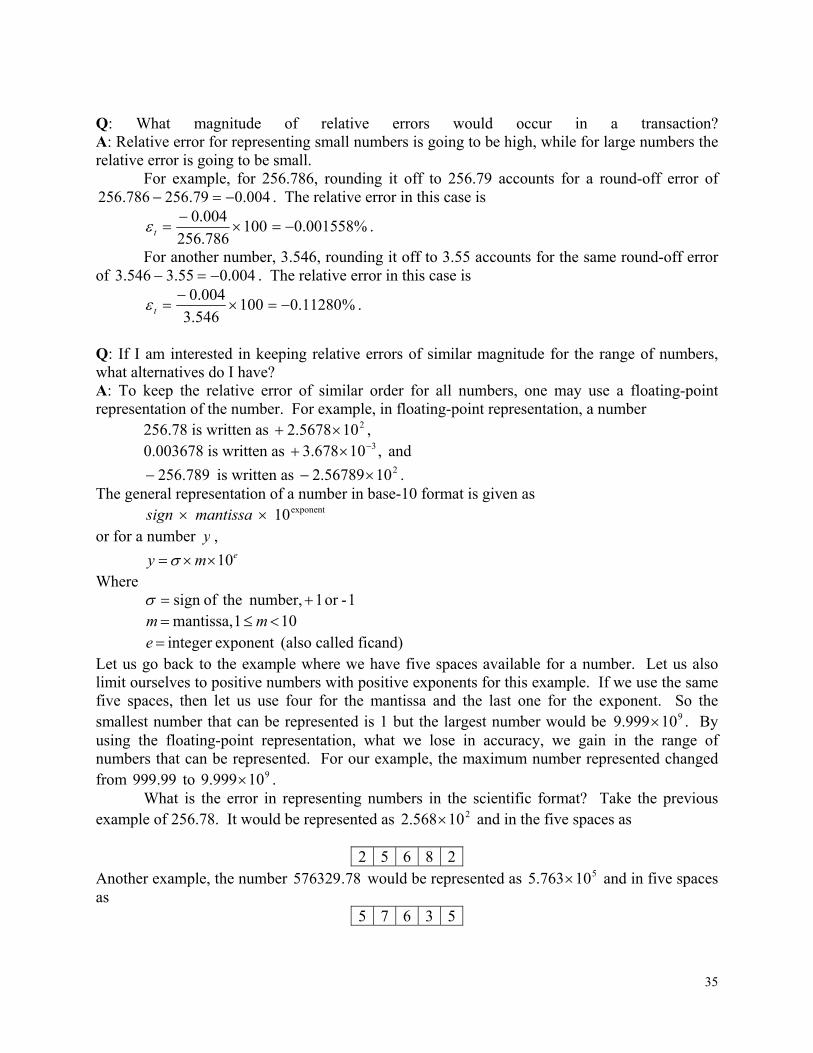
exponent integer e (also called ficand) Let us go back to the example where we have five spaces available for a number. Let us also limit ourselves to positive numbers with positive exponents for this example. If we use the same five spaces, then let us use four for the mantissa and the last one for the exponent. So the smallest number that can be represented is 1 but the largest number would be 910999.9 . By using the floating-point representation, what we lose in accuracy, we gain in the range of numbers that can be represented. For our example, the maximum number represented changed from 99.999 to 910999.9 . What is the error in representing numbers in the scientific format? Take the previous example of 256.78. It would be represented as 210568.2 and in the five spaces as

2 5 6 8 2 Another example, the number 78.576329 would be represented as 510763.5 and in five spaces as

5 7 6 3 5

36

So, how much error is caused by such representation. In representing 256.78, the round off error created is 020825678256 ... , and the relative error is

%0077888.010078.256

02.0

t ,

In representing 78.576329 , the round off error created is 78.2910763.578.576329 5 , and the relative error is

%0051672.010078.576329

78.29t .

What you are seeing now is that although the errors are large for large numbers, but the relative errors are of the same order for both large and small numbers. Q: How does this floating-point format relate to binary format? A: A number y would be written as

emy 2 Where

= sign of number (negative or positive – use 0 for positive and 1 for negative), m = mantissa, 22 101 m , that is, 1010 21 m , and

e = integer exponent.

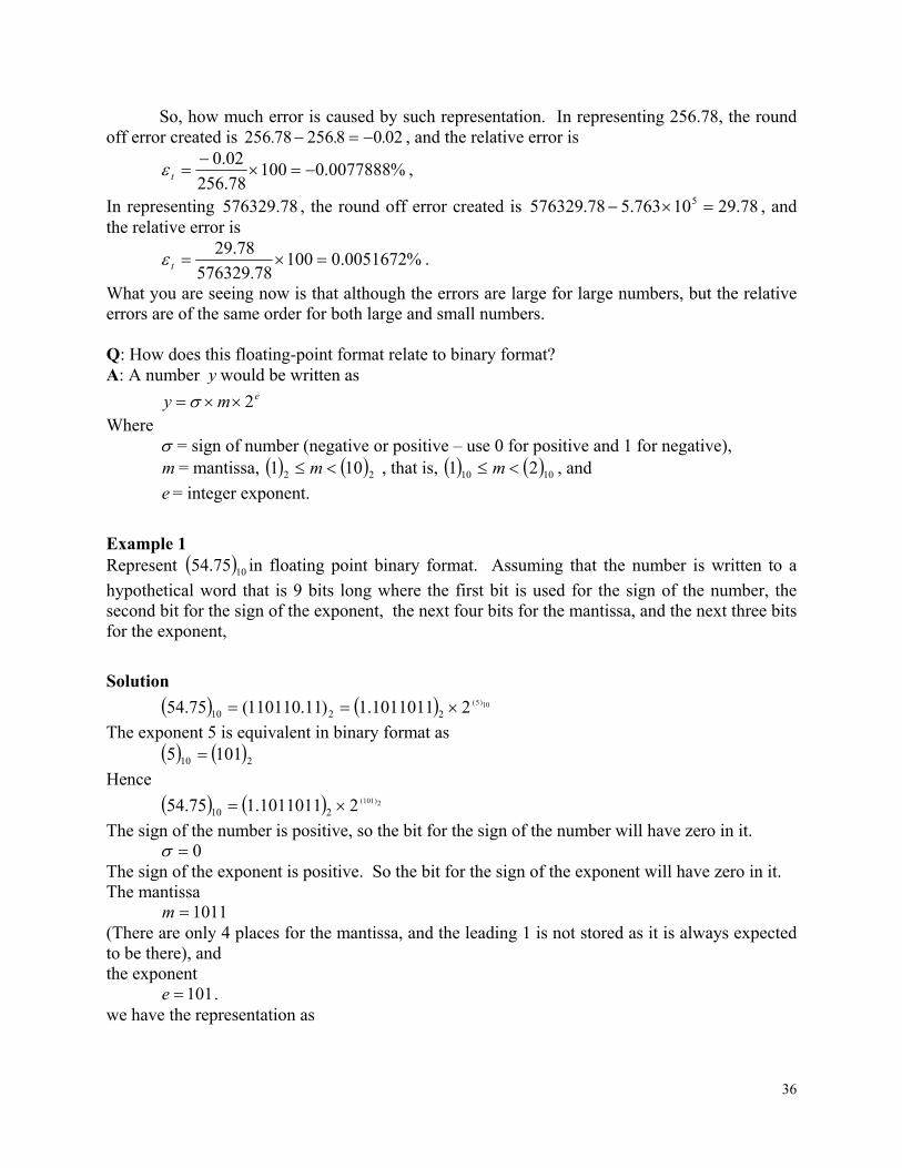
Example 1 Represent 1075.54 in floating point binary format. Assuming that the number is written to a

hypothetical word that is 9 bits long where the first bit is used for the sign of the number, the second bit for the sign of the exponent, the next four bits for the mantissa, and the next three bits for the exponent,

Solution

10)5(21011011.1)11.110110(75.54 2210

The exponent 5 is equivalent in binary format as 210 1015

Hence

2)101(21011011.175.54 210

The sign of the number is positive, so the bit for the sign of the number will have zero in it. 0

The sign of the exponent is positive. So the bit for the sign of the exponent will have zero in it. The mantissa

1011m (There are only 4 places for the mantissa, and the leading 1 is not stored as it is always expected to be there), and the exponent

101e . we have the representation as

37

0 0 1 0 1 1 1 0 1

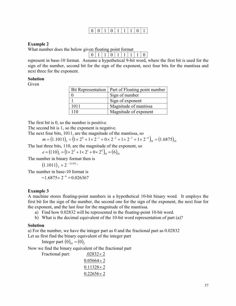
Example 2 What number does the below given floating point format

0 1 1 0 1 1 1 1 0 represent in base-10 format. Assume a hypothetical 9-bit word, where the first bit is used for the sign of the number, second bit for the sign of the exponent, next four bits for the mantissa and next three for the exponent.

Solution Given

Bit Representation Part of Floating point number 0 Sign of number 1 Sign of exponent 1011 Magnitude of mantissa 110 Magnitude of exponent

The first bit is 0, so the number is positive. The second bit is 1, so the exponent is negative. The next four bits, 1011, are the magnitude of the mantissa, so

101043210

2 6875.121212021211011.1 m

The last three bits, 110, are the magnitude of the exponent, so 1010

0122 6202121110 e

The number in binary format then is

21102 21011.1

The number in base-10 format is = 626875.1 0.026367

Example 3 A machine stores floating-point numbers in a hypothetical 10-bit binary word. It employs the first bit for the sign of the number, the second one for the sign of the exponent, the next four for the exponent, and the last four for the magnitude of the mantissa.

a) Find how 0.02832 will be represented in the floating-point 10-bit word. b) What is the decimal equivalent of the 10-bit word representation of part (a)?

Solution a) For the number, we have the integer part as 0 and the fractional part as 0.02832 Let us first find the binary equivalent of the integer part

Integer part 210 00

Now we find the binary equivalent of the fractional part Fractional part: 202832.

205664.0

211328.0

222656.0

38

245312.0

290624.0

281248.1

262496.1

224992.1

249984.0

299968.0

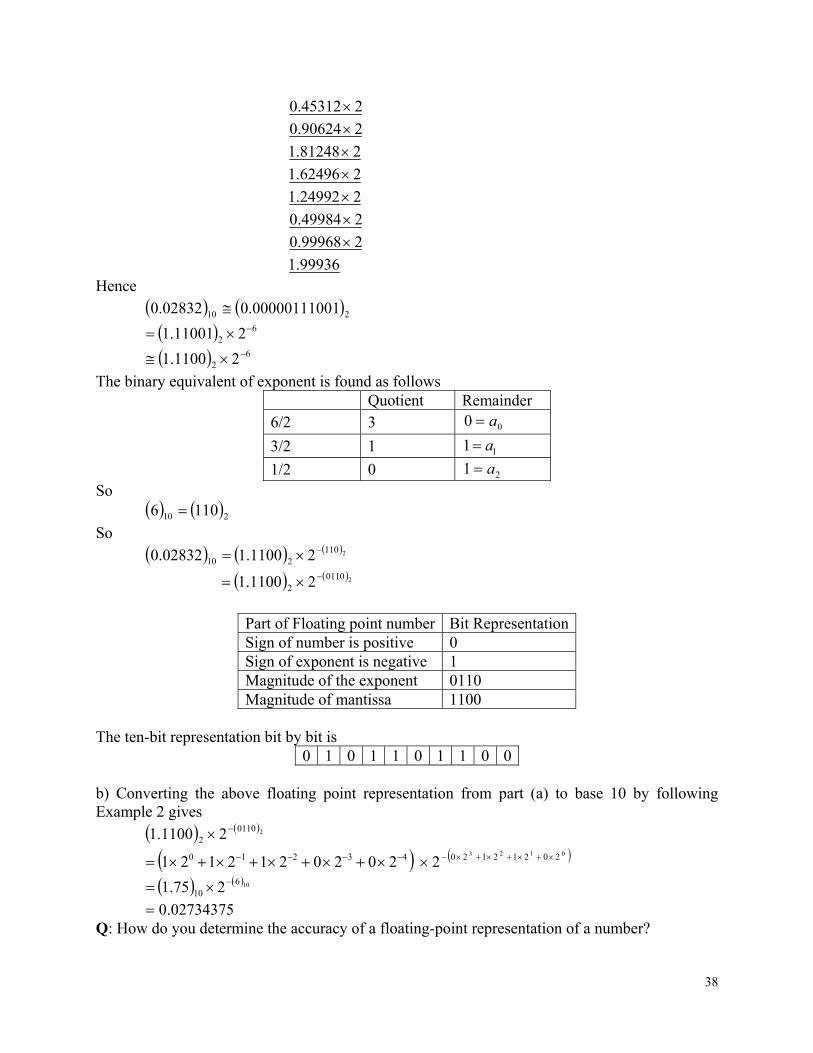
99936.1 Hence

210 10000011100.002832.0

62 211001.1

62 21100.1

The binary equivalent of exponent is found as follows Quotient Remainder 6/2 3 00 a

3/2 1 11 a

1/2 0 21 a So

210 1106

So

2110210 21100.102832.0

201102 21100.1

Part of Floating point number Bit Representation Sign of number is positive 0 Sign of exponent is negative 1 Magnitude of the exponent 0110 Magnitude of mantissa 1100

The ten-bit representation bit by bit is

0 1 0 1 1 0 1 1 0 0 b) Converting the above floating point representation from part (a) to base 10 by following Example 2 gives

201102 21100.1

43210 2020212121 0123 202121202

10610 275.1

02734375.0 Q: How do you determine the accuracy of a floating-point representation of a number?

39

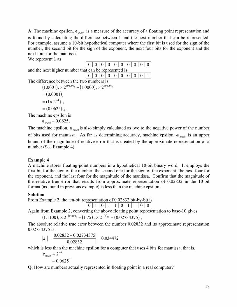
A: The machine epsilon, mach is a measure of the accuracy of a floating point representation and

is found by calculating the difference between 1 and the next number that can be represented. For example, assume a 10-bit hypothetical computer where the first bit is used for the sign of the number, the second bit for the sign of the exponent, the next four bits for the exponent and the next four for the mantissa. We represent 1 as

0 0 0 0 0 0 0 0 0 0 and the next higher number that can be represented is

0 0 0 0 0 0 0 0 0 1 The difference between the two numbers is

22 )0000(2

)0000(2 20000.120001.1

20001.0

104 )21(

10)0625.0( .

The machine epsilon is 0625.0mach .

The machine epsilon, mach is also simply calculated as two to the negative power of the number

of bits used for mantissa. As far as determining accuracy, machine epsilon, mach is an upper

bound of the magnitude of relative error that is created by the approximate representation of a number (See Example 4).

Example 4 A machine stores floating-point numbers in a hypothetical 10-bit binary word. It employs the first bit for the sign of the number, the second one for the sign of the exponent, the next four for the exponent, and the last four for the magnitude of the mantissa. Confirm that the magnitude of the relative true error that results from approximate representation of 0.02832 in the 10-bit format (as found in previous example) is less than the machine epsilon.

Solution From Example 2, the ten-bit representation of 0.02832 bit-by-bit is

0 1 0 1 1 0 1 1 0 0 Again from Example 2, converting the above floating point representation to base-10 gives

201102 21100.1 106

10 275.1 1002734375.0

The absolute relative true error between the number 0.02832 and its approximate representation 0.02734375 is

02832.0

02734375.002832.0 t 034472.0

which is less than the machine epsilon for a computer that uses 4 bits for mantissa, that is,

0625.0

2 4

mach.

Q: How are numbers actually represented in floating point in a real computer?

40

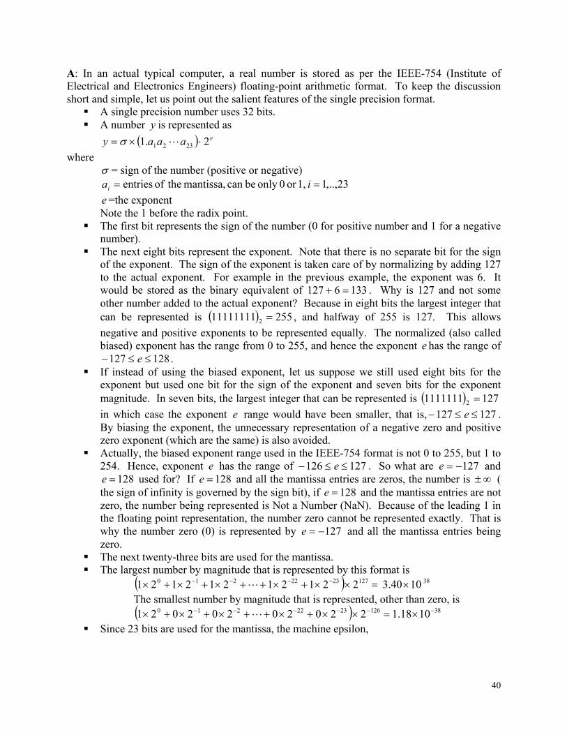
A: In an actual typical computer, a real number is stored as per the IEEE-754 (Institute of Electrical and Electronics Engineers) floating-point arithmetic format. To keep the discussion short and simple, let us point out the salient features of the single precision format. A single precision number uses 32 bits. A number y is represented as

eaaay 2.1 2321

where = sign of the number (positive or negative)

23,..,1 1,or 0only becan mantissa, theof entries iai

e =the exponent Note the 1 before the radix point. The first bit represents the sign of the number (0 for positive number and 1 for a negative

number). The next eight bits represent the exponent. Note that there is no separate bit for the sign

of the exponent. The sign of the exponent is taken care of by normalizing by adding 127 to the actual exponent. For example in the previous example, the exponent was 6. It would be stored as the binary equivalent of 1336127 . Why is 127 and not some other number added to the actual exponent? Because in eight bits the largest integer that can be represented is 25511111111 2 , and halfway of 255 is 127. This allows

negative and positive exponents to be represented equally. The normalized (also called biased) exponent has the range from 0 to 255, and hence the exponent e has the range of

128127 e . If instead of using the biased exponent, let us suppose we still used eight bits for the

exponent but used one bit for the sign of the exponent and seven bits for the exponent magnitude. In seven bits, the largest integer that can be represented is 1271111111 2

in which case the exponent e range would have been smaller, that is, 127127 e . By biasing the exponent, the unnecessary representation of a negative zero and positive zero exponent (which are the same) is also avoided.

Actually, the biased exponent range used in the IEEE-754 format is not 0 to 255, but 1 to 254. Hence, exponent e has the range of 127126 e . So what are 127e and

128e used for? If 128e and all the mantissa entries are zeros, the number is ( the sign of infinity is governed by the sign bit), if 128e and the mantissa entries are not zero, the number being represented is Not a Number (NaN). Because of the leading 1 in the floating point representation, the number zero cannot be represented exactly. That is why the number zero (0) is represented by 127e and all the mantissa entries being zero.

The next twenty-three bits are used for the mantissa. The largest number by magnitude that is represented by this format is

1272322210 22121212121 381040.3 The smallest number by magnitude that is represented, other than zero, is 1262322210 22020202021 381018.1 Since 23 bits are used for the mantissa, the machine epsilon,

41

7

23

1019.1

2

mach .

Q: How are numbers represented in floating point in double precision in a computer? A: In double precision IEEE-754 format, a real number is stored in 64 bits. The first bit is used for the sign, the next 11 bits are used for the exponent, and the rest of the bits, that is 52, are used for mantissa.

Can you find in double precision the range of the biased exponent, smallest number that can be represented, largest number that can be represented, and machine epsilon?

INTRODUCTION TO NUMERICAL METHODS Topic Floating Point Representation Summary Textbook notes on floating point representation Major General Engineering Authors Autar Kaw Date Aralık 8, 2016 Web Site http://numericalmethods.eng.usf.edu

42

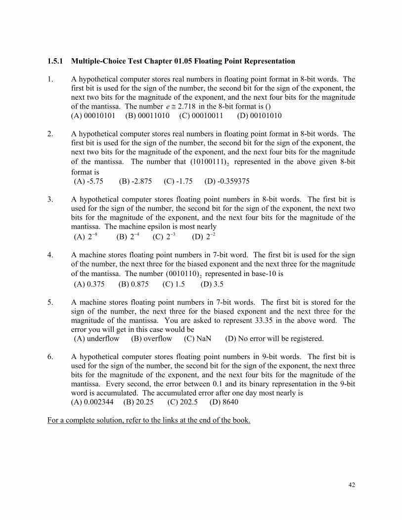
1.5.1 Multiple-Choice Test Chapter 01.05 Floating Point Representation 1. A hypothetical computer stores real numbers in floating point format in 8-bit words. The

first bit is used for the sign of the number, the second bit for the sign of the exponent, the next two bits for the magnitude of the exponent, and the next four bits for the magnitude of the mantissa. The number 718.2e in the 8-bit format is () (A) 00010101 (B) 00011010 (C) 00010011 (D) 00101010

2. A hypothetical computer stores real numbers in floating point format in 8-bit words. The

first bit is used for the sign of the number, the second bit for the sign of the exponent, the next two bits for the magnitude of the exponent, and the next four bits for the magnitude of the mantissa. The number that 2)10100111( represented in the above given 8-bit format is (A) -5.75 (B) -2.875 (C) -1.75 (D) -0.359375

3. A hypothetical computer stores floating point numbers in 8-bit words. The first bit is

used for the sign of the number, the second bit for the sign of the exponent, the next two bits for the magnitude of the exponent, and the next four bits for the magnitude of the mantissa. The machine epsilon is most nearly (A) 82 (B) 42 (C) 32 (D) 22

4. A machine stores floating point numbers in 7-bit word. The first bit is used for the sign

of the number, the next three for the biased exponent and the next three for the magnitude of the mantissa. The number 2)0010110( represented in base-10 is (A) 0.375 (B) 0.875 (C) 1.5 (D) 3.5

5. A machine stores floating point numbers in 7-bit words. The first bit is stored for the sign of the number, the next three for the biased exponent and the next three for the magnitude of the mantissa. You are asked to represent 33.35 in the above word. The error you will get in this case would be (A) underflow (B) overflow (C) NaN (D) No error will be registered.

6. A hypothetical computer stores floating point numbers in 9-bit words. The first bit is used for the sign of the number, the second bit for the sign of the exponent, the next three bits for the magnitude of the exponent, and the next four bits for the magnitude of the mantissa. Every second, the error between 0.1 and its binary representation in the 9-bit word is accumulated. The accumulated error after one day most nearly is (A) 0.002344 (B) 20.25 (C) 202.5 (D) 8640

For a complete solution, refer to the links at the end of the book.

43

1.6 Chapter 01.06 Propagation of Errors

PRE-REQUISITES

1. Know the definition of first derivative of a function (Primer for Differential Calculus). 2. Know how to find partial derivatives

OBJECTIVES

1. Find how errors propagate in arithmetic operations. 2. Quantify the errors based on individual components of an arithmetic operation or a

mathematical formula. If a calculation is made with numbers that are not exact, then the calculation itself will have an error. How do the errors in each individual number propagate through the calculations. Let’s look at the concept via some examples.

Example 1 Find the bounds for the propagation error in adding two numbers. For example if one is calculating YX where

05.05.1 X , 04.04.3 Y .

Solution By looking at the numbers, the maximum possible value of X and Y are

55.1X and 44.3Y Hence

99.444.355.1 YX is the maximum value of YX . The minimum possible value of X and Y are

45.1X and 36.3Y . Hence

36.345.1 YX 81.4 is the minimum value of YX . Hence

.99.481.4 YX One can find similar intervals of the bound for the other arithmetic operations of

YXYXYX /and,*, . What if the evaluations we are making are function evaluations instead? How do we find the value of the propagation error in such cases. If f is a function of several variables nn XXXXX ,,.......,,, 1321 , then the maximum

possible value of the error in f is

44

nn

nn

XX

fX

X

fX

X

fX

X

ff

11

22

11

.......

Example 2 The strain in an axial member of a square cross-section is given by

Eh

F2

where F =axial force in the member, N h = length or width of the cross-section, m E =Young’s modulus, Pa

Given N9.072F

mm1.04 h GPa5.170E

Find the maximum possible error in the measured strain. Solution

)1070()104(

72923

610286.64 286.64

EE

hh

FF

EhF 2

1

Eh

F

h 3

2

22 Eh

F

E

EEh

Fh

Eh

FF

Eh

2232

21

9

2923

933923

105.1)1070()104(

72

0001.0)1070()104(

7229.0

)1070()104(

1

667 103776.1102143.3100357.8 6103955.5 3955.5 Hence

)3955.5286.64(

45

implying that the axial strain, is between 8905.58 and 6815.69

Example 3 Subtraction of numbers that are nearly equal can create unwanted inaccuracies. Using the formula for error propagation, show that this is true.

Solution Let

yxz Then

yy

zx

x

zz

yx )1()1(

yx

So the absolute relative change is

yx

yx

z

z

As x and y become close to each other, the denominator becomes small and hence create large relative errors. For example if

001.02 x 001.0003.2 y

|003.22|

001.0001.0

z

z

= 0.6667 = 66.67% INTRODUCTION TO NUMERICAL METHODS Topic Propagation of Errors Summary Textbook notes on how errors propagate in arithmetic and

function evaluations Major All Majors of Engineering Authors Autar Kaw Last Revised Aralık 8, 2016 Web Site http://numericalmethods.eng.usf.edu

46

1.6.1 Multiple-Choice Test Chapter 01.06 Propagation of Errors 1. If 05.056.3 A and 04.025.3 B , the values of BA are

(A) 90.681.6 BA (B) 90.672.6 BA

(C) 81.681.6 BA (D) 91.671.6 BA 2. A number A is correctly rounded to 3.18 from a given number B . Then CBA ,

where C is (A) 0.005 (B) 0.01 (C) 0.18 (D) 0.09999

3. Two numbers A and B are approximated as C and D , respectively. The relative error

in DC is given by

(A)

B

DB

A

CA

(B)

B

DB

A

CA

B

DB

A

CA

(C)

B

DB

A

CA

B

DB

A

CA

(D)

B

DB

A

CA

4. The formula for normal strain in a longitudinal bar is given by AE

F where

F = normal force applied A = cross-sectional area of the bar E = Young’s modulus If N5.050 F , 2m002.02.0 A , and Pa10110210 99 E , the maximum error in the measurement of strain is

(A) 1210

(B) 111095.2 (C)

91022.1 (D) 91019.1

5. A wooden block is measured to be 60 mm by a ruler and the measurements are

considered to be good to 1/4th of a millimeter. Then in the measurement of 60 mm, we have ________ significant digits.

(A) 0 (B) 1 (C) 2 (D) 3 6. In the calculation of the volume of a cube of nominal size "5 , the uncertainty in the

measurement of each side is 10%. The uncertainty in the measurement of the volume would be

(A) 5.477% (B) 10.00% (C) 17.32% (D) 30.00% For a complete solution, refer to the links at the end of the book.

47

1.7 Chapter 01.07 Taylor’s Theorem Revisited

PRE-REQUISITES 1. Know the definition of derivatives of a function (Primer for Differential Calculus). 2. Know the derivatives of trigonometric and transcendental functions (Primer for

Differential Calculus).

OBJECTIVES 1. understand the basics of Taylor’s theorem, 2. write transcendental (karışık) and trigonometric functions as Taylor’s polynomial, 3. use Taylor’s theorem to find the values of a function at any point, given the values of the

function and all its derivatives at a particular point, 4. calculate errors and error bounds of approximating a function by Taylor series, and 5. revisit the chapter whenever Taylor’s theorem is used to derive or explain numerical

methods for various mathematical procedures.

After reading this chapter, you should be able to

1. understand the basics of Taylor’s theorem, 2. write transcendental and trigonometric functions as Taylor’s polynomial, 3. use Taylor’s theorem to find the values of a function at any point, given the values of the

function and all its derivatives at a particular point, 4. calculate errors and error bounds of approximating a function by Taylor series, and 5. revisit the chapter whenever Taylor’s theorem is used to derive or explain numerical

methods for various mathematical procedures. The use of Taylor series exists in so many aspects (yönleri) of numerical methods that it is imperative to devote (uzun süreçte) a separate chapter to its review and applications (Taylor serilerinin bütün yönleriyle sayısal yöntemlerde kullanıldığını görmek için ayrıntılı özetinin ve uygulamalarının ayrı bir bölüm halinde hazırlanması gerekmektedir). For example, you must have come across expressions such as (aşağıdaki ifadelerle karşılaşabilirsiniz)

!6!4!2

1)cos(642 xxx

x (1)

!7!5!3

)sin(753 xxx

xx (2)

!3!2

132 xx

xex (3)

All the above expressions are actually a special case (özel durumu) of Taylor series called the Maclaurin series. Why are these applications of Taylor’s theorem important for numerical methods? Expressions such as given in Equations (1), (2) and (3) give you a way to find the approximate values of these functions by using the basic arithmetic operations of addition, subtraction, division, and multiplication (toplama, çıkarma, çarpma ve bölme gibi basit aritmetik işlemleriyle fonksiyonların – iki sayı sisteminde işlem yapılabilecek şekilde - yazılması sağlanır).

48

Example 1 Find the value of 25.0e using the first five terms of the Maclaurin series (Maclaurin serisinin ilk beş terimi ile 25.0e değerini hesaplayınız ).

Solution The first five terms of the Maclaurin series for xe is

!4!3!21

432 xxxxex

!4

25.0

!3

25.0

!2

25.025.01

43225.0 e 2840.1

The exact value of 25.0e up to 5 significant digits is also 1.2840. But the above discussion and example do not answer our question of what a Taylor series is. Here it is, for a function xf

32

!3!2h

xfh

xfhxfxfhxf (4)

provided all derivatives of xf exist and are continuous between x and hx .

What does this mean in plain English? As Archimedes would have said (without the fine print), “Give me the value of the function at a single point, and the value of all (first, second, and so on) its derivatives, and I can give you the value of the function at any other point”. It is very important to note that the Taylor series is not asking for the expression of the function and its derivatives, just the value of the function and its derivatives at a single point. Now the fine print: Yes, all the derivatives have to exist and be continuous between x (the point where you are) to the point, hx where you are wanting to calculate the function at. However, if you want to calculate the function approximately by using the thn order Taylor polynomial, then thndst n,....,2,1 derivatives need to exist and be continuous in the closed interval

],[ hxx , while the thn )1( derivative needs to exist and be continuous in the open interval ),( hxx .

Example 2

Take xxf sin , we all know the value of 12

sin

. We also know the xxf cos and

02

cos

. Similarly )sin(xxf and 12

sin

. In a way, we know the value of xsin

and all its derivatives at 2

x . We do not need to use any calculators, just plain differential

calculus and trigonometry would do. Can you use Taylor series and this information to find the value of 2sin ?

Solution

49

2

x

2 hx xh 2

22

42920.0 So

!4

)(!3!2

432 hxf

hxf

hxfhxfxfhxf

2

x

42920.0h

xxf sin ,

2sin

2

f 1

xxf cos , 02

f

xxf sin , 12

f

)cos(xxf , 02

f

)sin(xxf , 12

f

Hence

!42!32!22222

432 hf

hf

hfhffhf

!4

42920.01

!3

42920.00

!2

42920.0142920.00142920.0

2

432f

00141393.00092106.001 90931.0 The value of 2sin I get from my calculator is 90930.0 which is very close to the value I just obtained. Now you can get a better value by using more terms of the series. In addition, you can now use the value calculated for 2sin coupled with the value of 2cos (which can be

calculated by Taylor series just like this example or by using the 1cossin 22 xx identity) to find value of xsin at some other point. In this way, we can find the value of xsin for any

value from 0x to 2 and then can use the periodicity of xsin , that is

,2,1,2sinsin nnxx to calculate the value of xsin at any other point.

Example 3

50

Derive the Maclaurin series of !7!5!3

sin753 xxx

xx

Solution

In the previous example, we wrote the Taylor series for xsin around the point 2

x .

Maclaurin series is simply a Taylor series for the point 0x . xxf sin , 00 f

xxf cos , 10 f

xxf sin , 00 f

xxf cos , 10 f

xxf sin , 00 f

)cos(xxf , 10 f Using the Taylor series now,

54!3!2

5432 hxf

hxf

hxf

hxfhxfxfhxf

5

04

0!3

0!2

00005432 h

fh

fh

fh

fhffhf

5

04

0!3

0!2

0005432 h

fh

fh

fh

fhffhf

5

14

0!3

1!2

0105432 hhhh

h

!5!3

53 hhh

So

!5!3

53 xxxxf

!5!3

sin53 xx

xx

Example 4 Find the value of 6f given that 1254 f , 744 f , 304 f , 64 f and all other

higher derivatives of xf at 4x are zero.

Solution

!3!2

32 hxf

hxfhxfxfhxf

4x 46 h

2

51

Since fourth and higher derivatives of xf are zero at 4x .

!3

24

!2

2424424

32

fffff

!3

26

!2

2302741256

32

f

860148125 341 Note that to find 6f exactly, we only needed the value of the function and all its derivatives at some other point, in this case, 4x . We did not need the expression for the function and all its derivatives. Taylor series application would be redundant if we needed to know the expression for the function, as we could just substitute 6x in it to get the value of 6f . Actually the problem posed above was obtained from a known function 523 23 xxxxf where 1254 f , 744 f , 304 f , 64 f , and all other

higher derivatives are zero.

Error in Taylor Series As you have noticed, the Taylor series has infinite terms. Only in special cases such as a finite polynomial does it have a finite number of terms. So whenever you are using a Taylor series to calculate the value of a function, it is being calculated approximately. The Taylor polynomial of order n of a function )(xf with )1( n continuous derivatives in the domain ],[ hxx is given by

hxRn

hxf

hxfhxfxfhxf n

nn

!!2''

2

where the remainder is given by

cfn

hhxR n

n

n1

1

)!1(

.

where hxcx

that is, c is some point in the domain hxx , .

Example 5 The Taylor series for xe at point 0x is given by

!5!4!3!2

15432 xxxx

xe x

a) What is the truncation (true) error in the representation of 1e if only four terms of the series are used? b) Use the remainder theorem to find the bounds of the truncation error.

Solution a) If only four terms of the series are used, then

52

!3!21

32 xxxe x

!3

1

!2

111

321 e 66667.2

The truncation (true) error would be the unused terms of the Taylor series, which then are

!5!4

54 xxEt

!5

1

!4

1 54

0516152.0

b) But is there any way to know the bounds of this error other than calculating it directly? Yes,

hxRn

hxfhxfxfhxf n

nn

!

where

cfn

hhxR n

n

n1

1

!1

, hxcx , and

c is some point in the domain hxx , . So in this case, if we are using four terms of the Taylor

series, the remainder is given by 3,0 nx

cfR 1313

3 !13

110

cf 4

!4

1

24

ce

Since hxcx 100 c

10 c The error is bound between

24

124

1

3

0 eR

e

24

124

13

eR

113261.01041667.0 3 R

So the bound of the error is less than 113261.0 which does concur with the calculated error of 0516152.0 .

Example 6 The Taylor series for xe at point 0x is given by

53

!5!4!3!2

15432 xxxx

xe x

As you can see in the previous example that by taking more terms, the error bounds decrease and hence you have a better estimate of 1e . How many terms it would require to get an approximation of 1e within a magnitude of true error of less than 610 ?

Solution Using 1n terms of the Taylor series gives an error bound of

cfn

hhxR n

n

n1

1

!1

xexfhx )(,1,0

cfn

R nn

n1

1

!1

11

cn

en !1

1 1

Since hxcx 100 c

10 c

)!1(

1)!1(

1

n

eR

n n

So if we want to find out how many terms it would require to get an approximation of 1e within a magnitude of true error of less than 610 ,

610)!1(

n

e

en 610)!1(

310)!1( 6 n (as we do not know the value of e but it is less than 3). 9n

So 9 terms or more will get 1e within an error of 610 in its value. We can do calculations such as the ones given above only for simple functions. To do a similar analysis of how many terms of the series are needed for a specified accuracy for any general function, we can do that based on the concept of absolute relative approximate errors discussed in Chapter 01.02 as follows. We use the concept of absolute relative approximate error (see Chapter 01.02 for details), which is calculated after each term in the series is added. The maximum value of m , for which the absolute relative approximate error is less than m 2105.0 % is the least number of significant digits correct in the answer. It establishes the accuracy of the approximate value of a function without the knowledge of remainder of Taylor series or the true error.

54

INTRODUCTION TO NUMERICAL METHODS Topic Taylor Theorem Revisited Summary These are textbook notes on Taylor Series Major All engineering majors Authors Autar Kaw Date Aralık 8, 2016 Web Site http://numericalmethods.eng.usf.edu

1.7.1 Multiple-Choice Test Chapter 01.07 Taylors Series Revisited 1. The coefficient of the 5x term in the Maclaurin polynomial for x2sin is

(A) 0 (B) 0.0083333 (C) 0.016667 (D) 0.26667 2. Given 63 f , 83 f , 113 f , and that all other higher order derivatives of

xf are zero at 3x , and assuming the function and all its derivatives exist and are

continuous between 3x and 7x , the value of 7f is (A) 38.000 (B) 79.500 (C) 126.00 (D) 331.50

3. Given that xy is the solution to 23 ydx

dy, 3)0( y the value of 2.0y from a

second order Taylor polynomial written around 0x is (A) 4.400 (B) 8.800 (C) 24.46 (D) 29.00

4. The series

0

2

4)!2(

1n

nn

n

n

x is a Maclaurin series for the following function

(A) xcos (B) x2cos (C) xsin (D) x2sin 5. The function

x

t dtexerf0

22

is called the error function. It is used in the field of probability and cannot be calculated exactly for finite values of x . However, one can expand the integrand as a Taylor polynomial and conduct integration. The approximate value of 0.2erf using the first three terms of the Taylor series around 0t is

(A) -0.75225 (B) 0.99532 (C) 1.5330 (D) 2.8586 6. Using the remainder of Maclaurin polynomial of thn order for xf defined as

xcncf

n

xxR n

n

n

0 ,0 ,!1

11

55

the least order of the Maclaurin polynomial required to get an absolute true error of at most 610 in the calculation of 1.0sin is (do not use the exact value of )1.0sin( or cos(0.1) to find the answer, but the knowledge that 1)sin( |x| and 1|)cos(| x ).

(A) 3 (B) 5 (C) 7 (D) 9 For a complete solution, refer to the links at the end of the book.

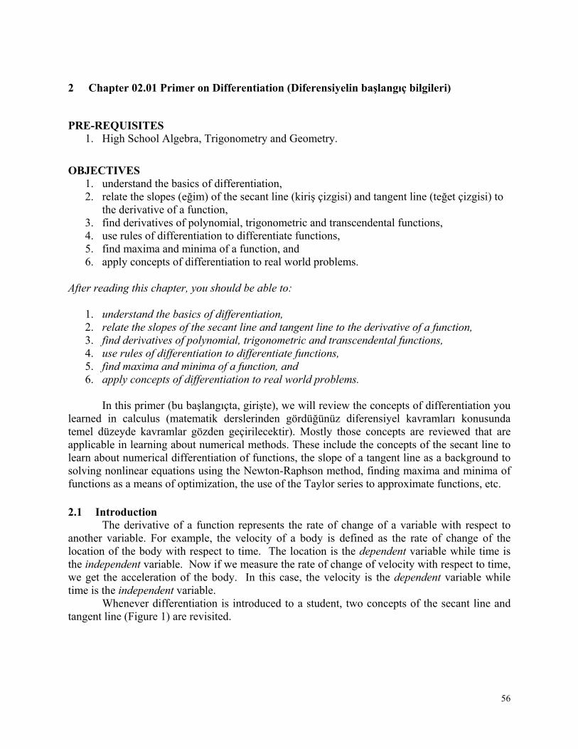
56

2 Chapter 02.01 Primer on Differentiation (Diferensiyelin başlangıç bilgileri)

PRE-REQUISITES 1. High School Algebra, Trigonometry and Geometry.

OBJECTIVES 1. understand the basics of differentiation, 2. relate the slopes (eğim) of the secant line (kiriş çizgisi) and tangent line (teğet çizgisi) to

the derivative of a function, 3. find derivatives of polynomial, trigonometric and transcendental functions, 4. use rules of differentiation to differentiate functions, 5. find maxima and minima of a function, and 6. apply concepts of differentiation to real world problems.

After reading this chapter, you should be able to:

1. understand the basics of differentiation, 2. relate the slopes of the secant line and tangent line to the derivative of a function, 3. find derivatives of polynomial, trigonometric and transcendental functions, 4. use rules of differentiation to differentiate functions, 5. find maxima and minima of a function, and 6. apply concepts of differentiation to real world problems.

In this primer (bu başlangıçta, girişte), we will review the concepts of differentiation you learned in calculus (matematik derslerinden gördüğünüz diferensiyel kavramları konusunda temel düzeyde kavramlar gözden geçirilecektir). Mostly those concepts are reviewed that are applicable in learning about numerical methods. These include the concepts of the secant line to learn about numerical differentiation of functions, the slope of a tangent line as a background to solving nonlinear equations using the Newton-Raphson method, finding maxima and minima of functions as a means of optimization, the use of the Taylor series to approximate functions, etc. 2.1 Introduction The derivative of a function represents the rate of change of a variable with respect to another variable. For example, the velocity of a body is defined as the rate of change of the location of the body with respect to time. The location is the dependent variable while time is the independent variable. Now if we measure the rate of change of velocity with respect to time, we get the acceleration of the body. In this case, the velocity is the dependent variable while time is the independent variable. Whenever differentiation is introduced to a student, two concepts of the secant line and tangent line (Figure 1) are revisited.

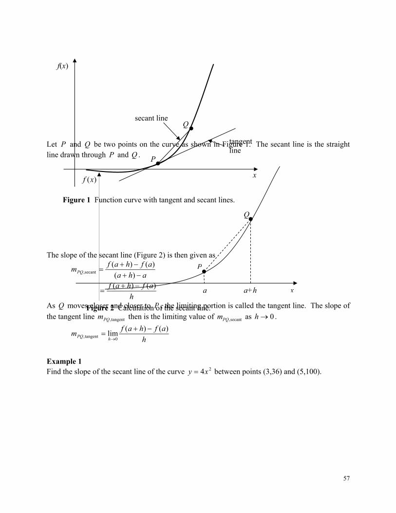
57

Let P and Q be two points on the curve as shown in Figure 1. The secant line is the straight line drawn through P and Q .

The slope of the secant line (Figure 2) is then given as

aha

afhafmPQ

)(

)()(secant,

h

afhaf )()(

As Q moves closer and closer to P , the limiting portion is called the tangent line. The slope of

the tangent line tangent,PQm then is the limiting value of secant,PQm as 0h .

h

afhafm

hPQ

)()(lim

0tangent,

Example 1 Find the slope of the secant line of the curve 24xy between points (3,36) and (5,100).

Q

P

f(x)

x

secant line

tangent line

Figure 1 Function curve with tangent and secant lines.

x

P

Q

a a+h

)(xf

Figure 2 Calculation of the secant line.

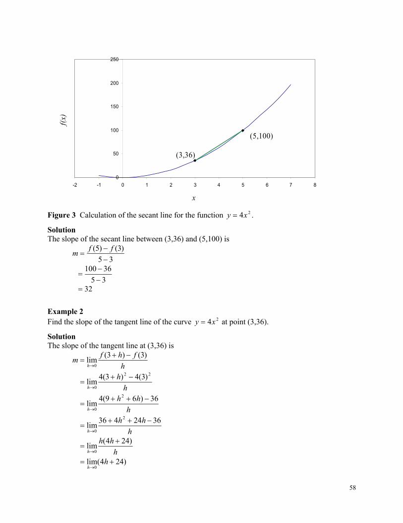
58

0

50

100

150

200

250

-2 -1 0 1 2 3 4 5 6 7 8

x

f(x)

(5,100)

(3,36)

Figure 3 Calculation of the secant line for the function 24xy .

Solution The slope of the secant line between (3,36) and (5,100) is

35

)3()5(

ff

m

35

36100

32

Example 2 Find the slope of the tangent line of the curve 24xy at point (3,36).

Solution The slope of the tangent line at (3,36) is

h

fhfm

h

)3()3(lim

0

h

hh

22

0

)3(4)3(4lim

h

hhh

36)69(4lim

2

0

h

hhh

3624436lim

2

0

h

hhh

)244(lim

0

)244(lim0

hh

59

24

0

10

20

30

40

50

60

70

-2 -1 0 1 2 3 4 5

x

f(x)

Figure 4 Calculation of the tangent line in the function 24xy .

The slope of the tangent line is

h

fhfm

h

)3()3(lim

0

h

hh

22

0

)3(4)3(4lim

h

hhh

3642436lim

2

0

h

hhh

)424(lim

0

)424(lim

0h

h

24

Derivative of a Function Recall from calculus, the derivative of a function )(xf at ax is defined as

h

afhafaf

h

)()(lim)(

0

Example 3 Find )3(f if 24)( xxf .

60

Solution

h

fhff

h

)3()3(lim)3(

0

h

hh

22

0

)3(4)3(4lim

h

hhh

36)69(4lim

2

0

h

hhh

3624436lim

2

0

h

hhh

)244(lim

0

)244(lim0

hh

24

Example 4

Find

4

f if )2()( xsinxf

Solution

h

fhff

h

44lim4 0

h

sinhsin

h

42

42

lim0

h

sinhsin

h

22

2lim

0

h

sinhsincoshcossin

h

2)2(

2)2(

2lim

0

h

hcosh

10)2(lim

0

h

hcosh

1)2(lim

0

0 from knowing that

0)(1

lim0

h

hcosh

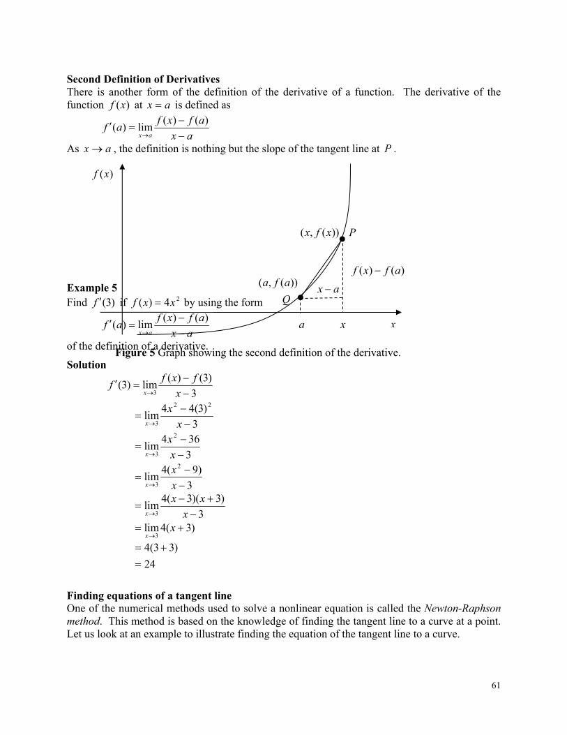
61

Second Definition of Derivatives There is another form of the definition of the derivative of a function. The derivative of the function )(xf at ax is defined as

ax

afxfaf

ax

)()(lim)(

As ax , the definition is nothing but the slope of the tangent line at P .

Example 5 Find )3(f if 24)( xxf by using the form

ax

afxfaf

ax

)()(lim)(

of the definition of a derivative.

Solution

3

)3()(lim)3(

3

x

fxff

x

3

)3(44lim

22

3

x

xx

3

364lim

2

3

x

xx

3

)9(4lim

2

3

x

xx

3

)3)(3(4lim

3

x

xxx

)3(4lim3

xx

24

)33(4

Finding equations of a tangent line One of the numerical methods used to solve a nonlinear equation is called the Newton-Raphson method. This method is based on the knowledge of finding the tangent line to a curve at a point. Let us look at an example to illustrate finding the equation of the tangent line to a curve.

)(xf

P

Q

))(,( afa

a

))(,( xfx

ax

)()( afxf

x

Figure 5 Graph showing the second definition of the derivative.

x

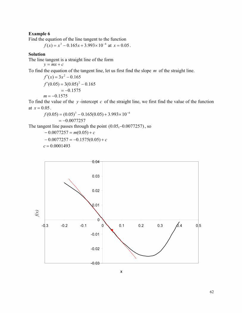
62

Example 6 Find the equation of the line tangent to the function 43 10993.3165.0)( xxxf at 05.0x .

Solution The line tangent is a straight line of the form cmxy To find the equation of the tangent line, let us first find the slope m of the straight line.

165.03)( 2 xxf 165.0)05.0(3)05.0( 2 f 1575.0 1575.0m To find the value of the y -intercept c of the straight line, we first find the value of the function at 05.0x . 43 10993.3)05.0(165.0)05.0()05.0( f 0077257.0 The tangent line passes through the point )0077257.0,05.0( , so

c

cm

)05.0(1575.00077257.0

)05.0(0077257.0

0001493.0c

-0.03

-0.02

-0.01

0

0.01

0.02

0.03

0.04

-0.3 -0.2 -0.1 0 0.1 0.2 0.3 0.4 0.5

x

f(x)

63

Figure 6 Graph of function f(x) and the tangent line at x = 0.05. Hence, cmxy 0001493.01575.0 x is the equation of the tangent line.

Other Notations of Derivatives Derivates can be denoted in several ways. For the first derivative, the notations are

dx

dyandyxf

dx

dxf , ),( ),(

For the second derivative, the notations are

2

2

2

2

, ),( ),(dx

ydandyxf

dx

dxf

For the thn derivative, the notations are

n

nn

n

nn

dx

ydyxf

dx

dxf , ),( ),( )()(

Theorems of Differentiation Several theorems of differentiation are given to show how one can find the derivative of different functions.

Theorem 1 The derivative of a constant is zero. If kxf )( , where k is a constant, 0)( xf .

Example 7 Find the derivative of 6)( xf .

Solution 6)( xf 0)( xf

Theorem 2 The derivative of nxxf )( , where 0n is 1)( nnxxf .

Example 8 Find the derivative of 6)( xxf .

Solution 6)( xxf

166)( xxf

56x

64

Example 9 Find the derivative of 6)( xxf .

Solution 6)( xxf

166)( xxf

76 x

7

6

x

Theorem 3 The derivative of )()( xkgxf , where k is a constant is )()( xgkxf .

Example 10 Find the derivative of 610)( xxf .

Solution 610)( xxf

)10()( 6xdx

dxf

610 xdx

d

)6(10 5x

560x Theorem 4 The derivative of )()()( xvxuxf is )()()( xvxuxf .

Example 11 Find the derivative of 83)( 3 xxf .

Solution

83)( 3 xxf

)83()( 3 x

dx

dxf

)8()3( 3

dx

dx

dx

d

0)(3 3 x

dx

d

)3(3 2x

65

29x

Theorem 5 The derivative of )()()( xvxuxf is

)()()()()( xudx

dxvxv

dx

dxuxf . (Product Rule)

Example 12 Find the derivative of )83)(62()( 32 xxxf

Solution Using the product rule as given by Theorem 5 where, )()()( xvxuxf

)()()()()( xudx

dxvxv

dx

dxuxf

)83)(62()( 32 xxxf

62)( 2 xxu

83)( 3 xxv Taking the derivative of )(xu ,

)62( 2 xdx

d

dx

du

)6()2( 2

dx

dx

dx

d

0)(2 2 xdx

d

)2(2 x x4 Taking the derivative of )(xv ,

)83( 3 xdx

d

dx

dv

)8()3( 3

dx

dx

dx

d

0)(3 3 xdx

d

)3(3 2x

29x Using the formula for the product rule

)()()()()( xudx

dxvxv

dx

dxuxf

66

xxx

xxxx

xxxx

325430

32125418

)4)(83()9)(62(

24

424

322

Theorem 6 The derivative of

)(

)()(

xv

xuxf

is

2))((

)()()()()(

xv

xvdx

dxuxu

dx

dxv

xf

(Quotient Rule)

Example 13

Find the derivative of )83(

)62()(

3

2

x

xxf .

Solution Use the quotient rule of Theorem 6, if

)(

)()(

xv

xuxf

then

2))((

)()()()()(

xv

xvdx

dxuxu

dx

dxv

xf

From

)83(

)62()(

3

2

x

xxf

we have 62)( 2 xxu

83)( 3 xxv Taking the derivative of )(xu ,

)62( 2 xdx

d

dx

du

)6()2( 2

dx

dx

dx

d

)2(2

0)(2 2

x

xdx

d

x4

67

Taking the derivative of )(xv ,

)83( 3 xdx

d

dx

dv

)8()3( 3

dx

dx

dx

d

)3(3

0)(3

2

3

x

xdx

d

29x Using the formula for the quotient rule,

23

223

)83(

)9)(62()4)(83()(

x

xxxxxf

64489

5418321236

244

xx

xxxx

64489

3254636

24

xx

xxx

Table of Derivatives

)(xf )(xf

0, nxn

1nnx

nkx , 0n 1nknx

)(xsin )(xcos

)(xcos )(xsin

)(xtan )(2 xsec

)(xsinh )(xcosh

)(xcosh )(xsinh

)(xtanh )(1 2 xtanh

)(1 xsin 21

1

x

)(1 xcos 21

1

x

)(1 xtan 21

1

x

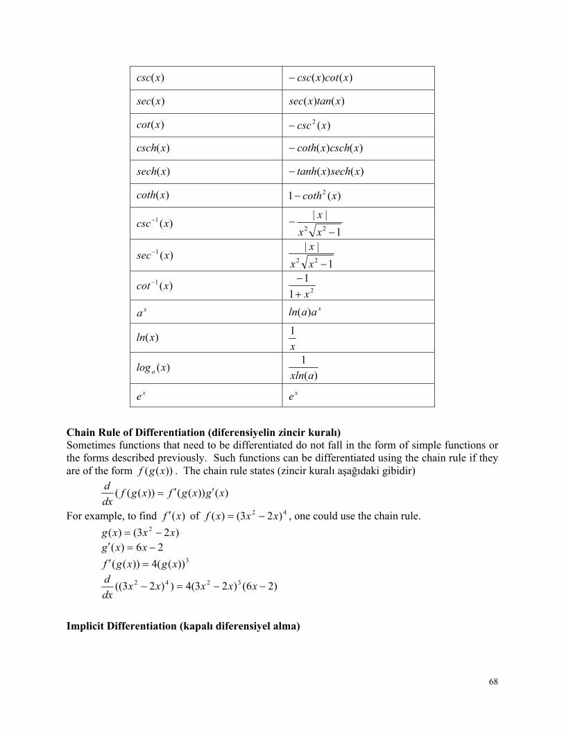
68

)(xcsc )()( xcotxcsc

)(xsec )()( xtanxsec

)(xcot )(2 xcsc

)(xcsch )()( xcschxcoth

)(xsech )()( xsechxtanh

)(xcoth )(1 2 xcoth

)(1 xcsc 1

||22

xx

x

)(1 xsec 1

||22 xx

x

)(1 xcot 21

1

x

xa

xaaln )(

)(xln x

1

)(xloga )(

1

axln xe

xe

Chain Rule of Differentiation (diferensiyelin zincir kuralı) Sometimes functions that need to be differentiated do not fall in the form of simple functions or the forms described previously. Such functions can be differentiated using the chain rule if they are of the form ))(( xgf . The chain rule states (zincir kuralı aşağıdaki gibidir)

)())(())((( xgxgfxgfdx

d

For example, to find )(xf of 42 )23()( xxxf , one could use the chain rule.

)23()( 2 xxxg 26)( xxg

3))((4))(( xgxgf

)26()23(4))23(( 3242 xxxxxdx

d

Implicit Differentiation (kapalı diferensiyel alma)

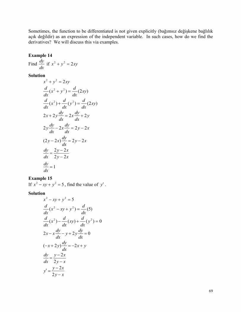
69

Sometimes, the function to be differentiated is not given explicitly (bağımsız değişkene bağlılık açık değildir) as an expression of the independent variable. In such cases, how do we find the derivatives? We will discuss this via examples.

Example 14

Find dx

dy if xyyx 222

Solution xyyx 222

)2()( 22 xydx

dyx

dx

d

)2()()( 22 xydx

dy

dx

dx

dx

d

ydx

dyx

dx

dyyx 2222

xydx

dyxy

xydx

dyx

dx

dyy

22)22(

2222

1

22

22

dx

dy

xy

xy

dx

dy

Example 15 If 522 yxyx , find the value of y .

Solution

522 yxyx

)5()( 22

dx

dyxyx

dx

d

0)()()( 22 y

dx

dxy

dx

dx

dx

d

022

dx

dyyy

dx

dyxx

yx

dx

dyyx 2)2(

xy

xy

dx

dy

2

2

xy

xyy

2

2

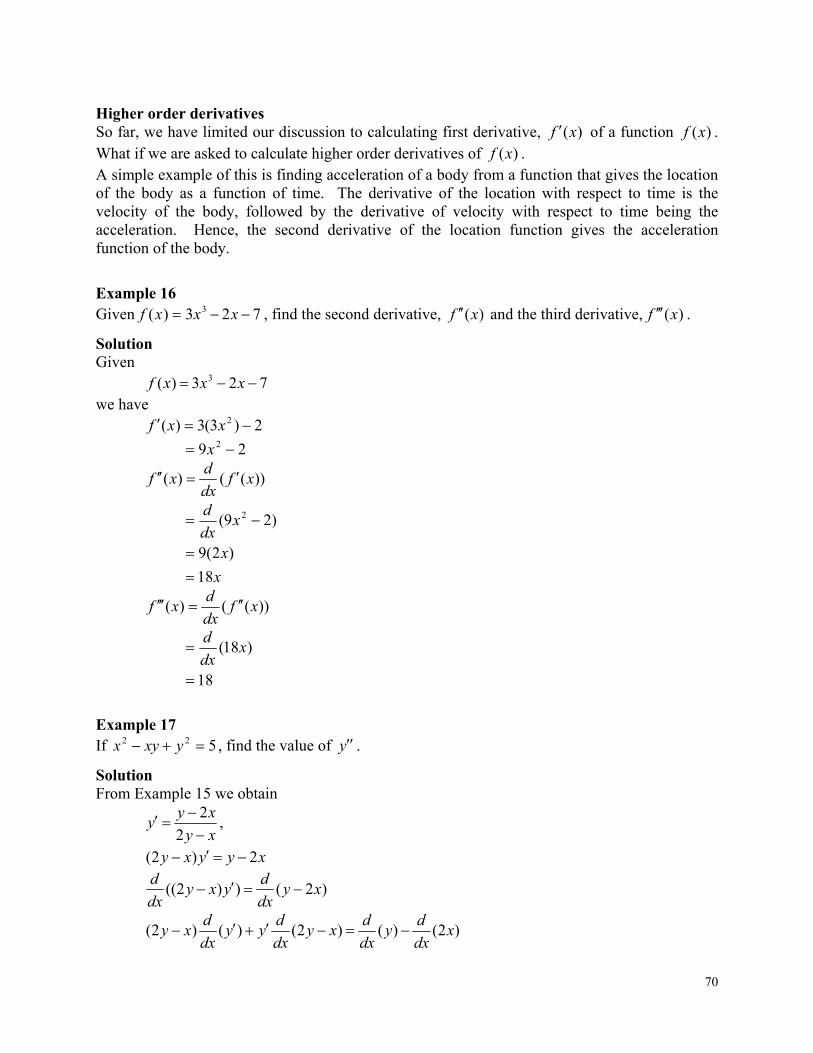
70

Higher order derivatives So far, we have limited our discussion to calculating first derivative, )(xf of a function )(xf . What if we are asked to calculate higher order derivatives of )(xf . A simple example of this is finding acceleration of a body from a function that gives the location of the body as a function of time. The derivative of the location with respect to time is the velocity of the body, followed by the derivative of velocity with respect to time being the acceleration. Hence, the second derivative of the location function gives the acceleration function of the body.

Example 16 Given 723)( 3 xxxf , find the second derivative, )(xf and the third derivative, )(xf .

Solution Given 723)( 3 xxxf we have 2)3(3)( 2 xxf

29 2 x

))(()( xfdx

dxf

x

x

xdx

d

18

)2(9

)29( 2

))(()( xfdx

dxf

18

)18(

xdx

d

Example 17 If 522 yxyx , find the value of y .

Solution From Example 15 we obtain

xy

xyy

2

2,

xyyxy 2)2(

)2())2(( xydx

dyxy

dx

d

)2()()2()()2( xdx

dy

dx

dxy

dx

dyy

dx

dxy

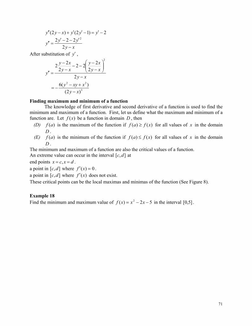
71

2)12()2( yyyxyy

xy

yyy

2

222 2

After substitution of y ,

xy

xy

xy

xy

xy

y

2

2

222

2

22

2

3

22

)2(

)(6

xy

xxyy

Finding maximum and minimum of a function The knowledge of first derivative and second derivative of a function is used to find the minimum and maximum of a function. First, let us define what the maximum and minimum of a function are. Let )(xf be a function in domain D , then

(D) )(af is the maximum of the function if )()( xfaf for all values of x in the domain D .

(E) )(af is the minimum of the function if )()( xfaf for all values of x in the domain D .

The minimum and maximum of a function are also the critical values of a function. An extreme value can occur in the interval ],[ dc at end points dxcx , . a point in ],[ dc where 0)( xf . a point in ],[ dc where )(xf does not exist. These critical points can be the local maximas and minimas of the function (See Figure 8).

Example 18 Find the minimum and maximum value of 52)( 2 xxxf in the interval ]5,0[ .

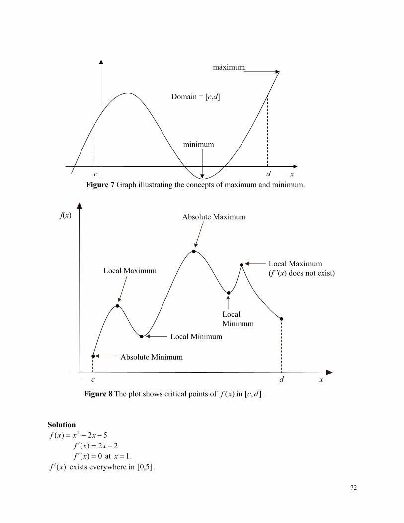
72

Solution 52)( 2 xxxf

22)( xxf 0)( xf at 1x .

)(xf exists everywhere in ]5,0[ .

f(x)

●

●

●

●

●

●

●

x

Figure 8 The plot shows critical points of )(xf in ],[ dc .

Absolute Minimum

Local Minimum

Local Minimum

Local Maximum (f´′(x) does not exist)

Absolute Maximum

Local Maximum

c d

maximum

minimum

x Figure 7 Graph illustrating the concepts of maximum and minimum.

Domain = [c,d]

c d

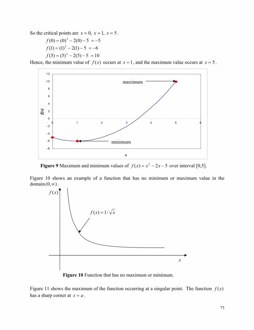
73

So the critical points are 5,1,0 xxx .

5)0(2)0()0( 2 f 5

5)1(2)1()1( 2 f 6

5)5(2)5()5( 2 f 10 Hence, the minimum value of )(xf occurs at 1x , and the maximum value occurs at 5x .

Figure 10 shows an example of a function that has no minimum or maximum value in the domain ),0( .

Figure 11 shows the maximum of the function occurring at a singular point. The function )(xf has a sharp corner at ax .

x

xxf /1)(

)(xf

Figure 10 Function that has no maximum or minimum.

-8

-6

-4

-2

0

2

4

6

8

10

12

0 1 2 3 4 5 6

x

f(x)

minimum

maximum

Figure 9 Maximum and minimum values of 52)( 2 xxxf over interval [0,5].

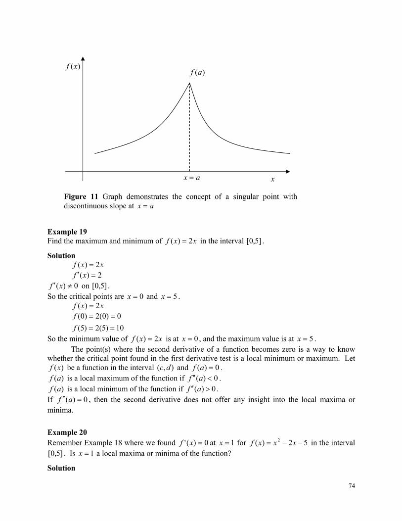
74

Example 19 Find the maximum and minimum of xxf 2)( in the interval ]5,0[ .

Solution xxf 2)( 2)( xf

0)( xf on ]5,0[ . So the critical points are 0x and 5x . xxf 2)(

10)5(2)5(

0)0(2)0(

f

f

So the minimum value of xxf 2)( is at 0x , and the maximum value is at 5x . The point(s) where the second derivative of a function becomes zero is a way to know whether the critical point found in the first derivative test is a local minimum or maximum. Let

)(xf be a function in the interval ),( dc and 0)( af . )(af is a local maximum of the function if 0)( af . )(af is a local minimum of the function if 0)( af .

If 0)( af , then the second derivative does not offer any insight into the local maxima or minima.

Example 20 Remember Example 18 where we found 0)(' xf at 1x for 52)( 2 xxxf in the interval

]5,0[ . Is 1x a local maxima or minima of the function?

Solution

)(xf

x

)(af

ax

Figure 11 Graph demonstrates the concept of a singular point with discontinuous slope at ax

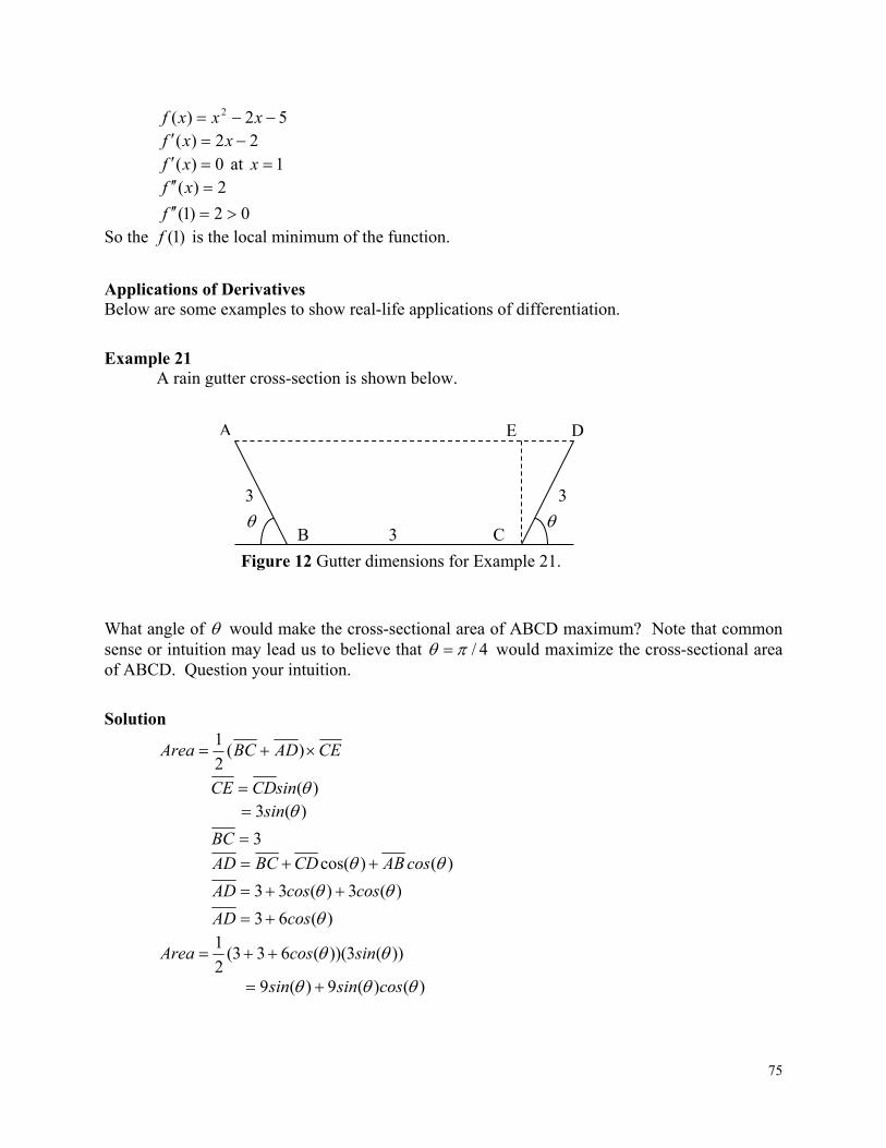
75

52)( 2 xxxf 22)( xxf 0)( xf at 1x

02)1(

2)(

f

xf

So the )1(f is the local minimum of the function.

Applications of Derivatives Below are some examples to show real-life applications of differentiation.

Example 21 A rain gutter cross-section is shown below.

What angle of would make the cross-sectional area of ABCD maximum? Note that common sense or intuition may lead us to believe that 4/ would maximize the cross-sectional area of ABCD. Question your intuition.

Solution

CEADBCArea )(2

1

)(sinCDCE )(3 sin

3BC

)()cos( cosABCDBCAD

)(3)(33 coscosAD

)(63 cosAD

))(3))((633(2

1 sincosArea

)()(9)(9 cossinsin

A

3

B C

D E

3

3

Figure 12 Gutter dimensions for Example 21.

76

)2(2

9)(9 sinsin

)2(22

9)(9

coscos

d

dA

)2(9)(9 coscos When is

0d

dA?

0)2(9)(9 coscos

3

The angle at which the area is maximum is 60 .

32

2

9

39

3

sinsinArea

34

27

2

3

2

9

2

39

For the interval of ],0[ , the area at the end points is

0)(

0)0(

Area

Area

Example 22 A classic example of the application of differentiation is to find the dimensions of a circular cylinder for a specific volume but which uses the least amount of material. Do this classic problem for a volume of 39m .

Solution The total surface area, A of the cylinder is A = top surface + side surface + bottom surface 22 2 rrhr rhr 22 2 The volume, V of the cylinder is hrV 2 since 39mV . We can write

2

2

9

9

rh

hr

This gives the surface area just in terms of r as

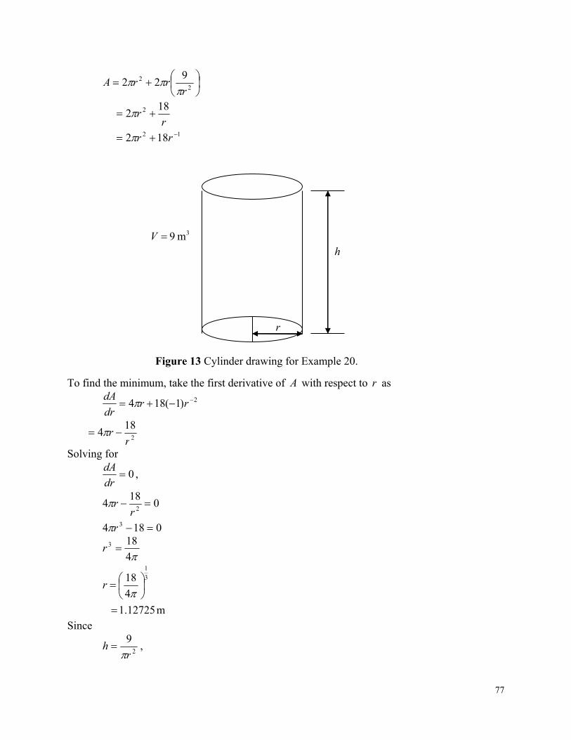
77

22 9

22r

rrA

12

2

182

182

rr

rr

To find the minimum, take the first derivative of A with respect to r as

2)1(184 rrdr

dA

2

184

rr

Solving for

0dr

dA,

0184

018

4

3

2

r

rr

4

183 r

m12725.1

4

18 3

1

r

Since

2

9

rh

,

Figure 13 Cylinder drawing for Example 20.

r

h

3m 9V

78

2)12725.1(

9

h m25450.2

But does this value of r correspond to a minimum?

32

2

)2(184 rdr

Ad

5025.4412725.1

364

364

3

r

This value 02

2

dr

Ad for m12725.1r . As per the second derivative test, m12725.1r

corresponds to a minimum.

DIFFERENTIATION Topic Primer on Differentiation Summary These are textbook notes of a primer on differentiation Major General Engineering Authors Autar Kaw, Luke Snyder Date July 17, 2008 Web Site http://numericalmethods.eng.usf.edu

Multiple-Choice Test Chapter 02.01 A Primer on Differentiation 1. The definition of the first derivative of a function )(xf is

(A) x

xfxxfxf

)()(

)(' (B) x

xfxxfxf

)()(

)('

(C) x

xfxxfxf

x

)()(lim)('

0 (D)

x

xfxxfxf

x

)()(lim)('

0

2. Given ,sin5 3 xey x dx

dy is

(A) xe x cos5 3 (B) xe x cos15 3 (C) xe x cos15 3 (D) xe x cos666.2 3

3. Given dx

dyxy ,2sin at 3x is most nearly

(A) 0.9600 (B) 0.9945 (C) 1.920 (D) 1.989

4. Given dx

dyxxy ,ln3 is

(A) xx ln3 2 (B) 22 ln3 xxx (C) 2x (D) x3

79

5. The velocity of a body as a function of time is given as 45 2 tet , where t is in seconds,

and is in m/s. The acceleration in 2m/s at 6.0t s is (A) -3.012 (B) 5.506 (C) 4.147 (D) -10.00

6. If 22 2 yxyx , then dx

dy is

(A) xy

yx

(B) yx 22 (C) y

x 1 (D) x

For a complete solution, refer to the links at the end of the book.

80

2.2 Chapter 02.02 Differentiation of Continuous Functions

PRE-REQUISITES 1. Know the definition of a secant, tangent to a function, and derivative of a function

(Primer for Differential Calculus). 2. Understand the representation of trigonometric and transcendental functions as a

Maclaurin series (Taylor Series Revisited).

OBJECTIVES 1. derive formulas for approximating the first derivative of a function, 2. derive formulas for approximating derivatives from Taylor series, 3. derive finite difference approximations for higher order derivatives, and 4. use the developed formulas in examples to find derivatives of a function.

After reading this chapter, you should be able to:

1. derive formulas for approximating the first derivative of a function, 2. derive formulas for approximating derivatives from Taylor series, 3. derive finite difference approximations for higher order derivatives, and 4. use the developed formulas in examples to find derivatives of a function.

The derivative of a function at x is defined as

x

xfxxfxf

x

0

lim

To be able to find a derivative numerically, one could make x finite to give,

x

xfxxfxf

.

Knowing the value of x at which you want to find the derivative of xf , we choose a value of

x to find the value of xf . To estimate the value of xf , three such approximations are suggested as follows.

Forward Difference Approximation of the First Derivative From differential calculus, we know

x

xfxxfxf

x

0

lim

For a finite x ,

x

xfxxfxf

The above is the forward divided difference approximation of the first derivative. It is called forward because you are taking a point ahead of x . To find the value of xf at ixx , we

may choose another point x ahead as 1 ixx . This gives

x

xfxfxf ii

i

1

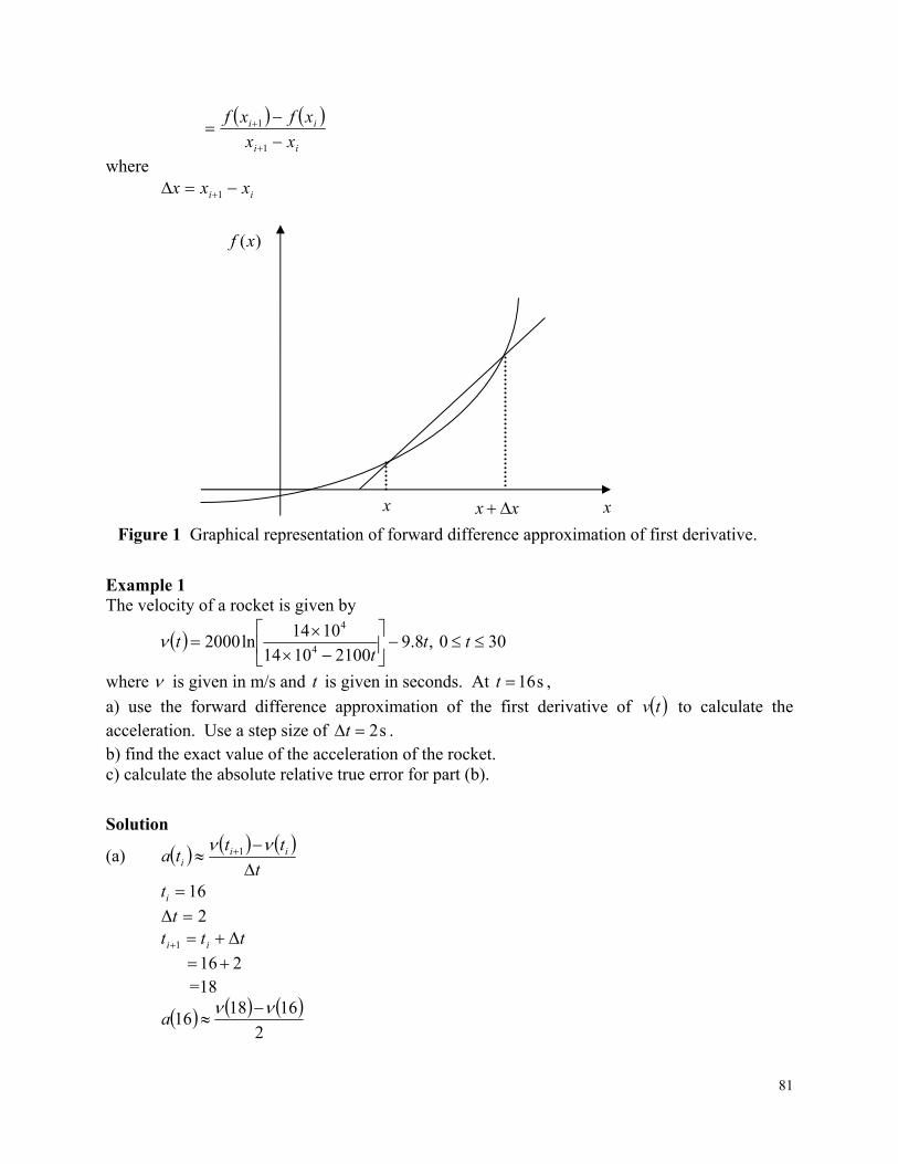
81

ii

ii

xx

xfxf

1

1

where ii xxx 1

Figure 1 Graphical representation of forward difference approximation of first derivative.

Example 1 The velocity of a rocket is given by

300 ,8.921001014

1014ln2000 4

4

tt

tt

where is given in m/s and t is given in seconds. At s16t ,

a) use the forward difference approximation of the first derivative of tν to calculate the acceleration. Use a step size of s2t . b) find the exact value of the acceleration of the rocket. c) calculate the absolute relative true error for part (b).

Solution

(a) t

ttta ii

i

1

16it

2Δ t ttt ii Δ1

216 =18

2

161816

a

)(xf

xx x x

82

188.91821001014

1014ln200018

4

4

m/s 02.453

168.91621001014

1014ln200016

4

4

m/s 07.392 Hence

2

161816

a

2

07.39202.453

2m/s474.30 (b) The exact value of 16a can be calculated by differentiating

tt

t 8.921001014

1014ln2000

4

4

as

tνdt

dta

Knowing that

t

tdt

d 1ln and

2

11

ttdt

d

8.921001014

1014

1014

210010142000

4

4

4

4

tdt

dtta

8.9210021001014

10141

1014

210010142000

24

4

4

4

t

t

t

t

3200

4.294040

163200

164.29404016

a

2m/s674.29 (c) The absolute relative true error is

100Value True

Value eApproximatValue True

t

100674.29

474.30674.29

%6967.2

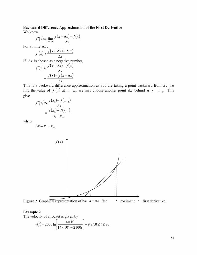
83

Backward Difference Approximation of the First Derivative We know

x

xfxxfxf

x

0

lim

For a finite x ,

x

xfxxfxf

If x is chosen as a negative number,

x

xfxxfxf

x

xxfxf

Δ

Δ

This is a backward difference approximation as you are taking a point backward from x . To find the value of xf at ixx , we may choose another point x behind as 1 ixx . This

gives

x

xfxfxf ii

i

1

1

1

ii

ii

xx

xfxf

where 1Δ ii xxx

Figure 2 Graphical representation of backward difference approximation of first derivative.

Example 2 The velocity of a rocket is given by

300,8.921001014

1014ln2000

4

4

tt

tt

)(xf

x xx x

84

(a) Use the backward difference approximation of the first derivative of tν to calculate the acceleration at s16t . Use a step size of s 2t . (b) Find the absolute relative true error for part (a).

Solution

t

ttta ii

1

16it

2Δ t ttt ii Δ1

216 = 14

2

141616

a

168.91621001014

1014ln200016

4

4

m/s07.392

148.91421001014

1014ln200014

4

4

m/s24.334

2

141616

a

2

24.33407.392

2m/s 915.28 (b) The exact value of the acceleration at s16t from Example 1 is

2m/s 674.2916 a The absolute relative true error for the answer in part (a) is

100674.29

915.28674.29

t

%5584.2

Forward Difference Approximation from Taylor Series Taylor’s theorem says that if you know the value of a function )(xf at a point ix and all its

derivatives at that point, provided the derivatives are continuous between ix and 1ix , then

2

111 !2 iii

iiiii xxxf

xxxfxfxf

Substituting for convenience ii xxx 1Δ

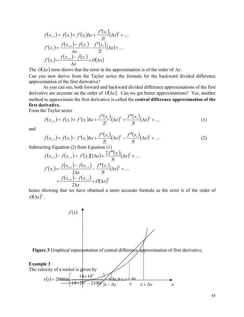
85

2

1 Δ!2

Δ xxf

xxfxfxf iiii

xxf

x

xfxfxf iii

i !21

xOx

xfxfxf ii

i

1

The xO term shows that the error in the approximation is of the order of x . Can you now derive from the Taylor series the formula for the backward divided difference approximation of the first derivative? As you can see, both forward and backward divided difference approximations of the first derivative are accurate on the order of xO . Can we get better approximations? Yes, another method to approximate the first derivative is called the central difference approximation of the first derivative. From the Taylor series

32

1 Δ!3

Δ!2

Δ xxf

xxf

xxfxfxf iiiii (1)

and

32

1 Δ!3

Δ!2

Δ xxf

xxf

xxfxfxf iiiii (2)

Subtracting Equation (2) from Equation (1)

3

11 Δ!3

2Δ2 x

xfxxfxfxf i

iii

211

!32x

xf

x

xfxfxf iii

i

211

2xO

x

xfxf ii

hence showing that we have obtained a more accurate formula as the error is of the order of

2xO .

Figure 3 Graphical representation of central difference approximation of first derivative.

Example 3 The velocity of a rocket is given by

300,8.921001014

1014ln2000

4

4

tt

tt .

)(xf

xx x xx x

86

(a) Use the central difference approximation of the first derivative of t to calculate the acceleration at s 16t . Use a step size of s 2t . (b) Find the absolute relative true error for part (a).

Solution

t

ttta ii

i

211

16it

2t

18

2161

ttt ii

14

2161

ttt ii

22

141816

a

4

1418 νν

188.91821001014

1014ln200018

4

4

m/s02.453

148.91421001014

1014ln200014

4

4

m/s24.334

4

141816

a

4

24.33402.453

2m/s 694.29 (b) The exact value of the acceleration at s 16t from Example 1 is 2m/s 674.2916 a The absolute relative true error for the answer in part (a) is

100674.29

694.29674.29

t

%069157.0 The results from the three difference approximations are given in Table 1.

Table 1 Summary of 16a using different difference approximations

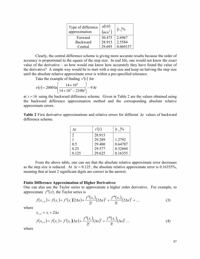
87

Type of difference approximation

16a

2m/s %t

Forward Backward

Central

30.475 28.915 29.695

2.6967 2.5584 0.069157

Clearly, the central difference scheme is giving more accurate results because the order of accuracy is proportional to the square of the step size. In real life, one would not know the exact value of the derivative – so how would one know how accurately they have found the value of the derivative? A simple way would be to start with a step size and keep on halving the step size until the absolute relative approximate error is within a pre-specified tolerance. Take the example of finding tv for

tt

t 8.921001014

1014ln2000

4

4

at 16t using the backward difference scheme. Given in Table 2 are the values obtained using the backward difference approximation method and the corresponding absolute relative approximate errors. Table 2 First derivative approximations and relative errors for different t values of backward difference scheme.

t tv %a

2 1 0.5 0.25 0.125

28.915 29.289 29.480 29.577 29.625

1.2792 0.64787 0.32604 0.16355

From the above table, one can see that the absolute relative approximate error decreases as the step size is reduced. At 125.0t , the absolute relative approximate error is 0.16355%, meaning that at least 2 significant digits are correct in the answer.

Finite Difference Approximation of Higher Derivatives One can also use the Taylor series to approximate a higher order derivative. For example, to approximate xf , the Taylor series is

32

2 Δ2!3

Δ2!2

Δ2 xxf

xxf

xxfxfxf iiiii (3)

where xxx ii Δ22

321 !3!2

xxf

xxf

xxfxfxf iiiii

(4)

where

88

xxx ii Δ1

Subtracting 2 times Equation (4) from Equation (3) gives

3212 ΔΔ2 xxfxxfxfxfxf iiiii

xxfx

xfxfxfxf i

iiii Δ

Δ

22

12

xOx

xfxfxfxf iii

i

212 2

(5)

Example 4 The velocity of a rocket is given by

300,8.921001014

1014ln2000

4

4

tt

tt

Use the forward difference approximation of the second derivative of t to calculate the jerk at s 16t . Use a step size of s 2t .

Solution

2

12 2

t

ttttj iii

i

16it

2t

18

2161

ttt ii

20

2216

22

ttt ii

22

161822016

j

208.92021001014

1014ln200020

4

4

m/s35.517

188.91821001014

1014ln200018

4

4

m/s02.453

168.91621001014

1014ln200016

4

4

m/s07.392

89

4

07.39202.453235.51716

j

3m/s 84515.0 The exact value of 16j can be calculated by differentiating

tt

t 8.921001014

1014ln2000

4

4

twice as

tνdt

dta and

tadt

dtj

Knowing that

t

tdt

d 1ln and

2

11

ttdt

d

8.921001014

1014

1014

210010142000

4

4

4

4

tdt

dtta

8.9210021001014

10141

1014

210010142000

24

4

4

4

t

t

t

t

3200

4.294040

Similarly it can be shown that

tadt

dtj

2)3200(

18000

t

3

2

m/s77909.0

)]16(3200[

1800016

j

The absolute relative true error is

10077909.0

84515.077909.0

t

%4797.8 The formula given by Equation (5) is a forward difference approximation of the second derivative and has an error of the order of xO . Can we get a formula that has a better accuracy? Yes, we can derive the central difference approximation of the second derivative.

90

The Taylor series is

...!4!3!2

4321

x

xfx

xfx

xfxxfxfxf iii

iii (6)

where xxx ii Δ1

432

1 !4!3!2x

xfx

xfx

xfxxfxfxf iii

iii (7)

where xxx ii Δ1

Adding Equations (6) and (7), gives

...

122

42

11

xxfxxfxfxfxf iiiii

...

12

2 2

211

xxf

x

xfxfxfxf iiii

i

2

211 2

xOx

xfxfxf iii

Example 5 The velocity of a rocket is given by

300 ,8.921001014

1014ln2000

4

4

tt

tt ,

(a) Use the central difference approximation of the second derivative of tν to calculate the jerk at s 16t . Use a step size of s 2t .

Solution The second derivative of velocity with respect to time is called jerk. The second order approximation of jerk then is

2

11 2

t

ttttj iiii

16it

2t

18

2161

ttt ii

14

2162

ttt ii

22

141621816

j

91

188.91821001014

1014ln200018

4

4

m/s02.453

168.91621001014

1014ln200016

4

4

m/s07.392

148.91421001014

1014ln200014

4

4

m/s24.334

22

141621816

j

4

24.33407.392202.453

3m/s 77969.0 The absolute relative true error is

10077908.0

77969.077908.0

t

%077992.0

DIFFERENTIATION Topic Differentiation of Continuous functions Summary These are textbook notes of differentiation of continuous functions Major General Engineering Authors Autar Kaw, Luke Snyder Date Aralık 8, 2016 Web Site http://numericalmethods.eng.usf.edu

2.3 Multiple-Choice Test Chapter 02.02 Differentiation of Continuous Functions 1. The definition of the first derivative of a function )(xf is

(A) x

xfxxfxf

)()(

)(' (B) x

xfxxfxf

)()(

)('

(C) x

xfxxfxf

x

)()(lim)('

0 (D)

x

xfxxfxf

x

)()(lim)('

0

2. The exact derivative of 3)( xxf at 5x is most nearly

(A) 25.00 (B) 75.00 (C) 106.25 (D) 125.00

92

3. Using the forwarded divided difference approximation with a step size of 0.2, the derivative of xexf 3.25)( at 25.1x is

(A) 163.4 (B) 203.8 (C) 211.1 (D) 258.8

4. A student finds the numerical value of 220.20)( xedx

d at 3x using a step size of 0.2.

Which of the following methods did the student use to conduct the differentiation? (A) Backward divided difference (B) Calculus, that is, exact (C) Central divided difference (D) Forward divided difference

5. Using the backward divided difference approximation, 3715.4)( xedx

d at 5.1x for a

step size of 0.05. If you keep halving the step size to find )( xedx

dat 5.1x before two

significant digits can be considered to be at least correct in your answer, the step size would be (you cannot use the exact value to determine the answer)

(A) 0.05/2 (B) 0.05/4 (C) 0.05/8 (D) 0.05/16 6. The heat transfer rate q over a surface is given by

dy

dTkAq

where

k = thermal conductivity

Kms

J

A = surface area 2m

T = temperature K

y = distance normal to the surface m Given

Kms

J025.0

k

2m 3A the temperature T over the surface varies as

500107622001493 23 yyyT The heat transfer rate q at the surface most nearly is

(A) -1076 W (B) 37.5 W (C) 80.7 W (D) 500 W For a complete solution, refer to the links at the end of the book.

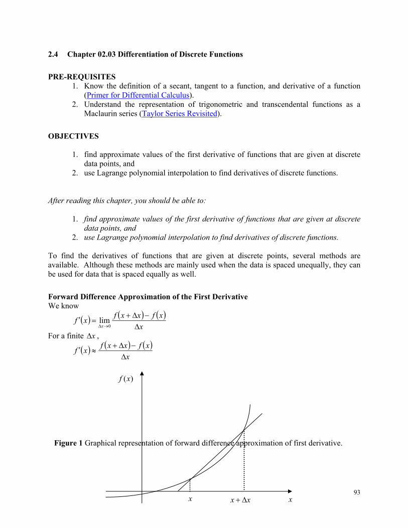
93

2.4 Chapter 02.03 Differentiation of Discrete Functions

PRE-REQUISITES 1. Know the definition of a secant, tangent to a function, and derivative of a function

(Primer for Differential Calculus). 2. Understand the representation of trigonometric and transcendental functions as a

Maclaurin series (Taylor Series Revisited).

OBJECTIVES

1. find approximate values of the first derivative of functions that are given at discrete data points, and

2. use Lagrange polynomial interpolation to find derivatives of discrete functions. After reading this chapter, you should be able to:

1. find approximate values of the first derivative of functions that are given at discrete data points, and

2. use Lagrange polynomial interpolation to find derivatives of discrete functions. To find the derivatives of functions that are given at discrete points, several methods are available. Although these methods are mainly used when the data is spaced unequally, they can be used for data that is spaced equally as well.

Forward Difference Approximation of the First Derivative We know

x

xfxxfxf

x

0

lim

For a finite x ,

x

xfxxfxf

Figure 1 Graphical representation of forward difference approximation of first derivative.

)(xf

xx x x

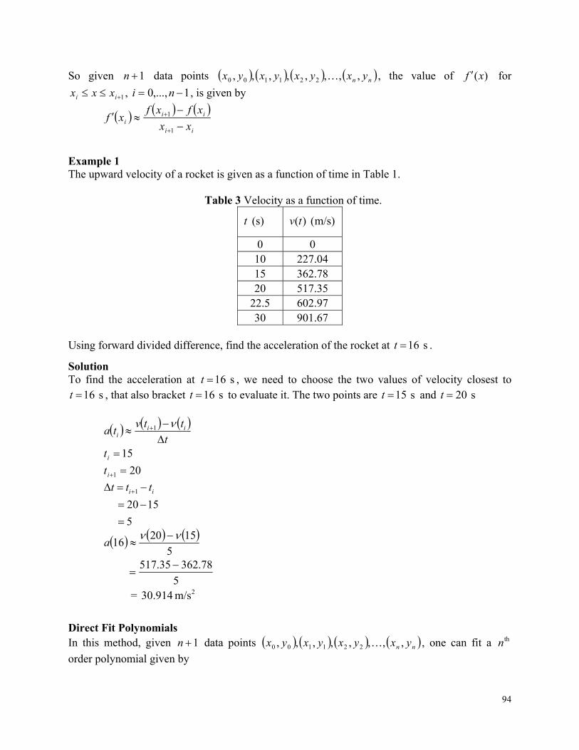
94

So given 1n data points nn yxyxyxyx ,,,,,,,, 221100 , the value of )(xf for

1 ii xxx , 1,...,0 ni , is given by

ii

iii xx

xfxfxf

1

1

Example 1 The upward velocity of a rocket is given as a function of time in Table 1.

Table 3 Velocity as a function of time.

(s) t )m/s( )(tv

0 0 10 227.04 15 362.78 20 517.35

22.5 602.97 30 901.67

Using forward divided difference, find the acceleration of the rocket at s 16t .

Solution To find the acceleration at s 16t , we need to choose the two values of velocity closest to

s 16t , that also bracket s 16t to evaluate it. The two points are s 15t and s 20t

t

ttvta iii

1

15it

201 it

5

1520 1

ii ttt

5

152016

a

5

78.36235.517

= 2m/s 30.914

Direct Fit Polynomials In this method, given 1n data points nn yxyxyxyx ,,,,,,,, 221100 , one can fit a thn

order polynomial given by

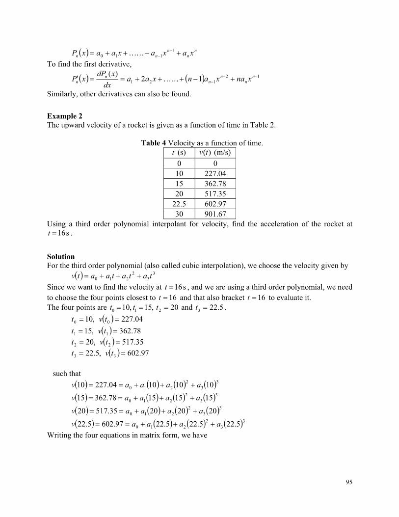
95

nn

nnn xaxaxaaxP

1110

To find the first derivative,

12121 12

)( n

nn

nn

n xnaxanxaadx

xdPxP

Similarly, other derivatives can also be found.

Example 2 The upward velocity of a rocket is given as a function of time in Table 2.

Table 4 Velocity as a function of time. (s) t )m/s( )(tv

0 0 10 227.04 15 362.78 20 517.35

22.5 602.97 30 901.67

Using a third order polynomial interpolant for velocity, find the acceleration of the rocket at s16t .

Solution For the third order polynomial (also called cubic interpolation), we choose the velocity given by 3

32

210 tatataatv

Since we want to find the velocity at s16t , and we are using a third order polynomial, we need to choose the four points closest to 16t and that also bracket 16t to evaluate it. The four points are ,15 ,10 10 tt 202 t and 5.223 t .

04.227,10 00 tvt

78.362,15 11 tvt

35.517,20 22 tvt

97.602,5.22 33 tvt

such that

332

210 10101004.22710 aaaav

332

210 15151578.36215 aaaav

332

210 20202035.51720 aaaav

332

210 5.225.225.2297.6025.22 aaaav

Writing the four equations in matrix form, we have

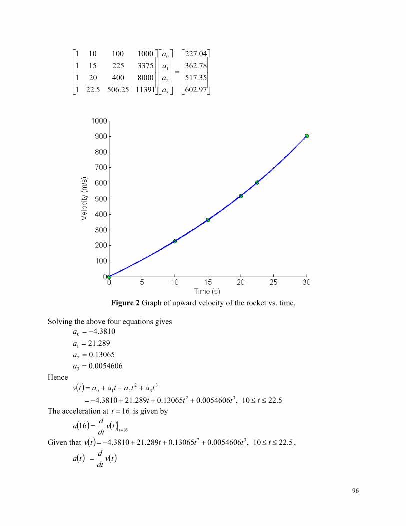
96

97.602

35.517

78.362

04.227

1139125.5065.221

8000400201

3375225151

1000100101

3

2

1

0

a

a

a

a

Figure 2 Graph of upward velocity of the rocket vs. time.

Solving the above four equations gives 3810.40 a

289.211 a

13065.02 a

0054606.03 a

Hence 3

32

210 tatataatv

5.2210 ,0054606.013065.0289.213810.4 32 tttt The acceleration at 16t is given by

16

16

t

tvdt

da

Given that 5.2210 ,0054606.013065.0289.213810.4 32 tttttv ,

tvdt

dta

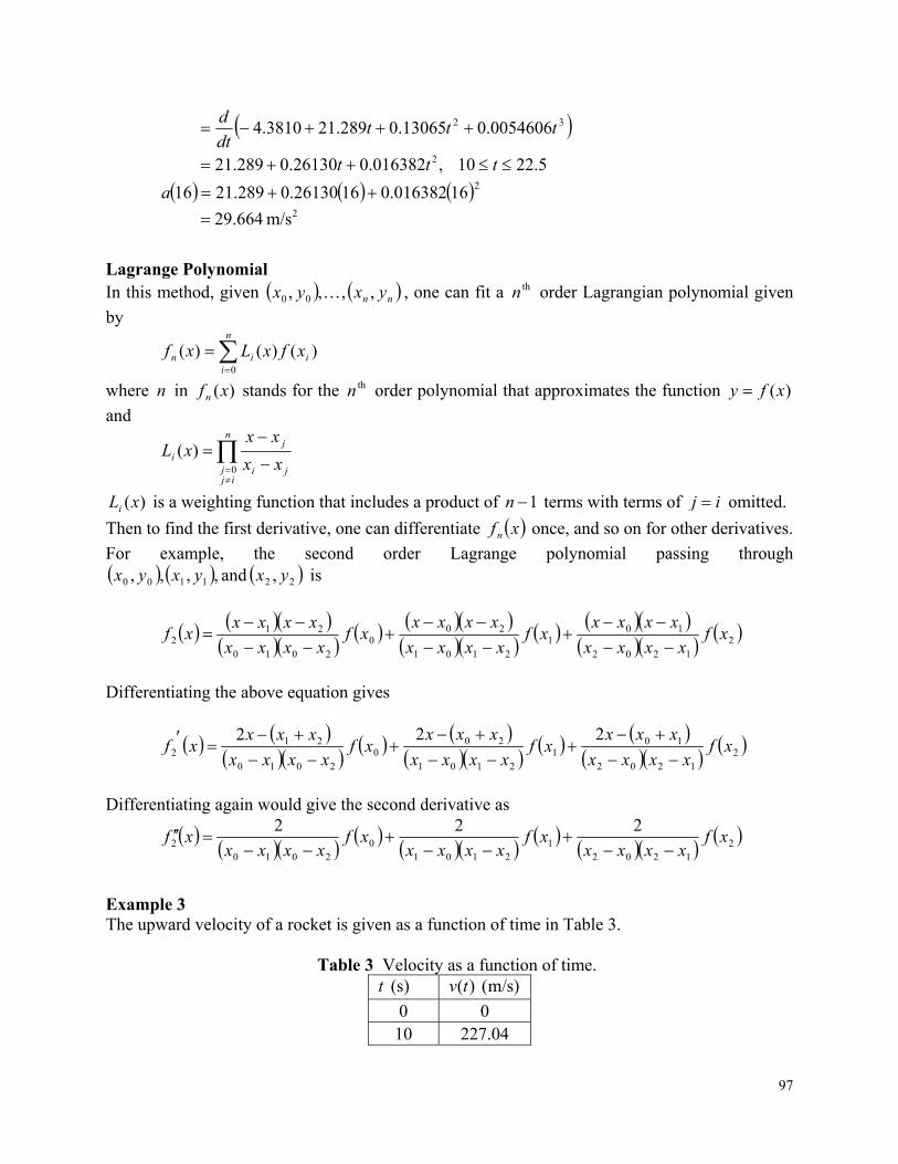
97

32 0054606.013065.0289.213810.4 tttdt

d

5.2210,016382.026130.0289.21 2 ttt

216016382.01626130.0289.2116 a

2m/s 664.29

Lagrange Polynomial In this method, given nn yxyx ,,,, 00 , one can fit a thn order Lagrangian polynomial given

by

n

iiin xfxLxf

0

)()()(

where n in )(xfn stands for the thn order polynomial that approximates the function )(xfy

and

n

ijj ji

ji xx

xxxL

0

)(

)(xLi is a weighting function that includes a product of 1n terms with terms of ij omitted.

Then to find the first derivative, one can differentiate xfn once, and so on for other derivatives.

For example, the second order Lagrange polynomial passing through 221100 , and ,,,, yxyxyx is

2

1202

101

2101

200

2010

212 xf

xxxx

xxxxxf

xxxx

xxxxxf

xxxx

xxxxxf

Differentiating the above equation gives

2

1202

101

2101

200

2010

212

222xf

xxxx

xxxxf

xxxx

xxxxf

xxxx

xxxxf

Differentiating again would give the second derivative as

21202

12101

02010

2

222xf

xxxxxf

xxxxxf

xxxxxf

Example 3 The upward velocity of a rocket is given as a function of time in Table 3.

Table 3 Velocity as a function of time.

(s) t )m/s( )(tv

0 0 10 227.04

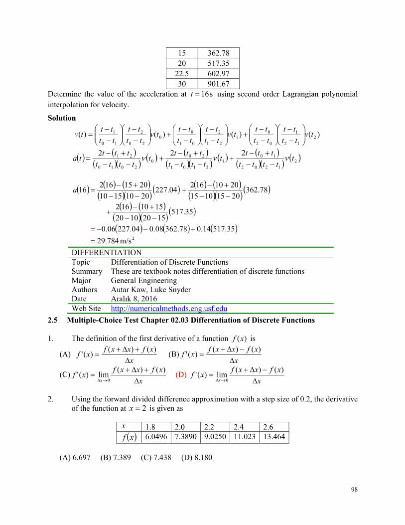
98

15 362.78 20 517.35

22.5 602.97 30 901.67

Determine the value of the acceleration at s16t using second order Lagrangian polynomial interpolation for velocity.

Solution

)()()()( 212

1

02

01

21

2

01

00

20

2

10

1 tvtt

tt

tt

tttv

tt

tt

tt

tttv

tt

tt

tt

tttv

0

2010

212t

tttt

tttta

12101

202t

tttt

ttt

21202

102t

tttt

ttt

04.227

20101510

201516216

a

78.36220151015

2010162

35.51715201020

1510162

35.51714.078.36208.004.22706.0

2m/s784.29

DIFFERENTIATION Topic Differentiation of Discrete Functions Summary These are textbook notes differentiation of discrete functions Major General Engineering Authors Autar Kaw, Luke Snyder Date Aralık 8, 2016 Web Site http://numericalmethods.eng.usf.edu

2.5 Multiple-Choice Test Chapter 02.03 Differentiation of Discrete Functions 1. The definition of the first derivative of a function )(xf is

(A) x

xfxxfxf

)()(

)(' (B)x

xfxxfxf

)()(

)('

(C)x

xfxxfxf

x

)()(lim)('

0 (D)

x

xfxxfxf

x

)()(lim)('

0

2. Using the forward divided difference approximation with a step size of 0.2, the derivative

of the function at 2x is given as

x

1.8 2.0 2.2 2.4 2.6 xf

6.0496 7.3890 9.0250 11.023 13.464

(A) 6.697 (B) 7.389 (C) 7.438 (D) 8.180

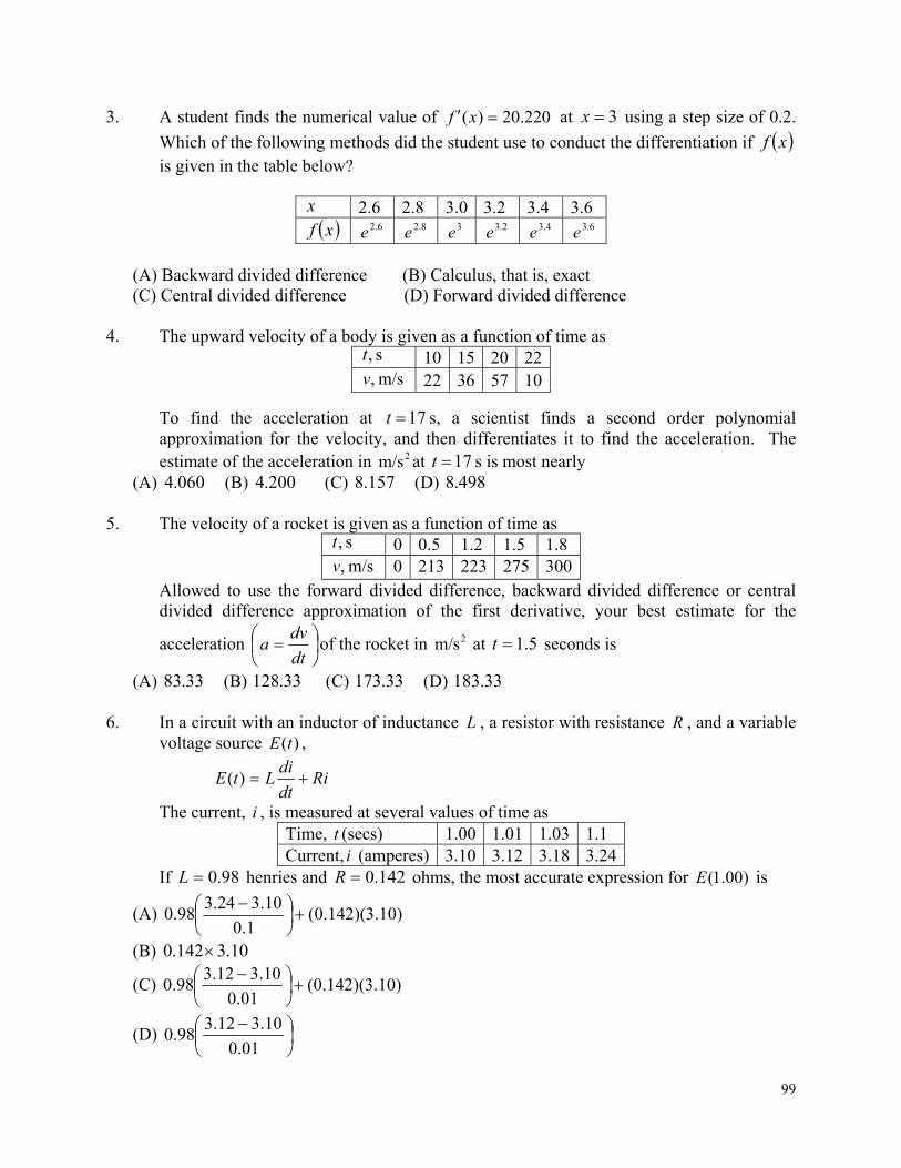
99

3. A student finds the numerical value of 220.20)( xf at 3x using a step size of 0.2.

Which of the following methods did the student use to conduct the differentiation if xf is given in the table below?

x

2.6 2.8 3.0 3.2 3.4 3.6 xf

6.2e

8.2e

3e

2.3e

4.3e

6.3e

(A) Backward divided difference (B) Calculus, that is, exact (C) Central divided difference (D) Forward divided difference

4. The upward velocity of a body is given as a function of time as To find the acceleration at 17t s, a scientist finds a second order polynomial approximation for the velocity, and then differentiates it to find the acceleration. The estimate of the acceleration in 2m/s at 17t s is most nearly

(A) 060.4 (B) 200.4 (C) 157.8 (D) 498.8 5. The velocity of a rocket is given as a function of time as

s ,t 0 0.5 1.2 1.5 1.8 m/s ,v 0 213 223 275 300

Allowed to use the forward divided difference, backward divided difference or central divided difference approximation of the first derivative, your best estimate for the

acceleration

dt

dva of the rocket in 2m/s at 5.1t seconds is

(A) 33.83 (B) 33.128 (C) 33.173 (D) 33.183 6. In a circuit with an inductor of inductance L , a resistor with resistance R , and a variable

voltage source )(tE ,

Ridt

diLtE )(

The current, i , is measured at several values of time as Time, t (secs) 1.00 1.01 1.03 1.1 Current, i (amperes) 3.10 3.12 3.18 3.24

If 98.0L henries and 142.0R ohms, the most accurate expression for )00.1(E is

(A) )10.3)(142.0(1.0

10.324.398.0

(B) 10.3142.0

(C) )10.3)(142.0(01.0

10.312.398.0

(D)

01.0

10.312.398.0

s ,t 10 15 20 22 m/s ,v 22 36 57 10

100

For a complete solution, refer to the links at the end of the book.

101

3 Chapter 03.01 Cubic Equations - Solution of Quadratic Equations

3.1 Solution of Quadratic Equations

PRE-REQUISITES (ön koşullar) 1. High School Algebra – Equations 2. Complex Algebra – Concept of complex numbers, Euler’s formula

OBJECTIVES (hedefler) 1. find the solutions of quadratic equations, 2. derive the formula for the solution of quadratic equations, 3. solve simple physical problems involving quadratic equations.

After reading this chapter, you should be able to:

1. find the solutions of quadratic equations, 2. derive the formula for the solution of quadratic equations, 3. solve simple physical problems involving quadratic equations.

What are quadratic equations and how do we solve them? A quadratic equation has the form

02 cbxax , where 0a The solution to the above quadratic equation is given by

a

acbbx

2

42

So the equation has two roots, and depending on the value of the discriminant, acb 42 , the equation may have real, complex or repeated roots. If 042 acb , the roots are complex. If 042 acb , the roots are real. If 042 acb , the roots are real and repeated.

Example 1 Derive the solution to 02 cbxax .

Solution 02 cbxax

Dividing both sides by a , 0a , we get

02 a

cx

a

bx

Note if 0a , the solution to 02 cbxax is

102

b

cx

Rewrite

02 a

cx

a

bx

as

042 2

22

a

c

a

b

a

bx

a

c

a

b

a

bx

2

22

42

2

2

4

4

a

acb

2

2

4

4

2 a

acb

a

bx

a

acb

2

42

a

acb

a

bx

2

4

2

2

a

acbb

2

42

Example 2 A ball is thrown down at 50 mph from the top of a building. The building is 420 feet tall. Derive the equation that would let you find the time the ball takes to reach the ground.

Solution The distance s covered by the ball is given by

2

2

1gtuts

where u = initial velocity (ft/s) g = acceleration due to gravity ( 2ft/s ) t = time )(s

Given

mile 1

ft 5280

s 3600

hour 1

hour

miles50 u

s

ft 73.33

2s

ft32.2g

ft 420s

103

we have

2 2.322

1 73.33 420 tt

04203373116 2 t.t. The above equation is a quadratic equation, the solution of which would give the time it would take the ball to reach the ground. The solution of the quadratic equation is

870.7,315.3

)1.16(2

)420(1.16433.7333.73 2

t

Since ,0t the valid value of time t is s 3.315 .

NONLINEAR EQUATIONS Topic Solution of quadratic equations Summary Textbook notes on solving quadratic equations Major General Engineering Authors Autar Kaw Date Aralık 8, 2016 Web Site http://numericalmethods.eng.usf.edu

3.1.1 Multiple-Choice Test Chapter 03.01 Background Nonlinear Equations 1. The value of x that satisfies 0xf is called the

(A) root of an equation 0xf (B) root of a function xf

(C) zero of an equation 0xf (D) none of the above 2. A quadratic equation has ________ root(s).

(A) one (B) two (C) three (D) four 3. For a certain cubic equation, at least one of the roots is known to be a complex root.

How many total complex roots does the cubic equation have? (A) one (B) two (C) three (D) cannot be determined

4. An equation such as xx tan has _________ root(s).

(A) zero (B) one (C) two (D) infinite 5. A polynomial of order n has __________ zeros.

(A) 1n (B) n (C) 1n (D) 2n 6. The velocity of a body is given by 45)( tetv , where t is in seconds and v is in sm .

The velocity of the body is 6 sm at t = _____ seconds. (A) 0.1823 (B) 0.3979 (C) 0.9163 (D) 1.609

For a complete solution, refer to the links at the end of the book.

104

3.2 Chapter 03.02 Solution of Cubic Equations

PRE-REQUISITES

1. Know how to manipulate equations. 2. Know how to find solution of quadratic equations (Solution of Quadratic Equations) 3. Know basics of complex numbers (Complex numbers – Trusted External link) 4. Know Euler’s formula (Euler’s formula – Trusted External link)

OBJECTIVES

1. find the exact solution of a general cubic equation. After reading this chapter, you should be able to:

1. find the exact solution of a general cubic equation.

How to Find the Exact Solution of a General Cubic Equation In this chapter, we are going to find the exact solution of a general cubic equation

023 dcxbxax (1) To find the roots of Equation (1), we first get rid of the quadratic term 2x by making the substitution

a

byx

3 (2)

to obtain

0333

23

d

a

byc

a

byb

a

bya (3)

Expanding Equation (3) and simplifying, we obtain the following equation

0327

2

3 2

323

a

bc

a

bdy

a

bcay (4)

Equation (4) is called the depressed cubic since the quadratic term is absent. Having the equation in this form makes it easier to solve for the roots of the cubic equation (Click here to know the history behind solving cubic equations exactly). First, convert the depressed cubic Equation (4) into the form

0327

21

3

12

323

a

bc

a

bd

ay

a

bc

ay

03 feyy (5) where

105

a

bc

ae

3

1 2

a

bc

a

bd

af

327

212

3

Now, reduce the above equation using Vieta’s substitution

z

szy (6)

For the time being, the constant s is undefined. Substituting into the depressed cubic Equation (5), we get

03

f

z

sze

z

sz (7)

Expanding out and multiplying both sides by 3z , we get 033 32346 szessfzzesz (8)

Now, let 3

es ( s is no longer undefined) to simplify the equation into a tri-quadratic equation.

027

336

efzz (9)

By making one more substitution, 3zw , we now have a general quadratic equation which can be solved using the quadratic formula.

027

32

efww (10)

Once you obtain the solution to this quadratic equation, back substitute using the previous substitutions to obtain the roots to the general cubic equation.

xyzw where we assumed

3zw (11)

z

szy

3

es (12)

a

byx

3

Note: You will get two roots for w as Equation (10) is a quadratic equation. Using

(11)Equation would then give you three roots for each of the two roots of w , hence giving you six root values for z . But the six root values of z would give you six values of y ( (6)Equation ); but three values of y will be identical to the other three. So one gets only three values of y , and hence three values of x . (Equation (2))

Example 1

106

Find the roots of the following cubic equation. 080369 23 xxx

Solution For the general form given by Equation (1)

023 dcxbxax we have

1a , 9b , 36c , 80d in

080369 23 xxx (E1-1) Equation (E1-1) is reduced to

03 feyy where

a

bc

ae

3

1 2

13

936

1

1 2

9 and

a

bc

a

bd

af

327

212

3

13

369

127

9280

1

12

3

26 giving

02693 yy (E1-2) For the general form given by Equation (5)

03 feyy we have

9e , 26f in Equation (E1-2). From Equation (12)

3

es

3

9

3 From Equation (10)

027

32

efww

107

027

926

32 ww

027262 ww where

3zw and

z

szy

z

z3

12

27142626 2 w

1,27 The solution is

271 w

12 w Since

3zw wz 3

For 1ww

13 wz

27 027 ie Since

3zw

iii euuere 333

3sin3cossincos 3 iuir resulting in

3ur 3coscos 3sinsin

Since sin and cos are periodic of 2 , k 23

3

2 k

k will take the value of 0, 1 and 2 before repeating the same values of . So,

2 ,1 ,0 ,3

2

k

k

31

108

3

22

3

43

So roots of 3zw are

3sin

3cos3

1

1

irz

3

2sin

3

2cos3

1

2

irz

3

4sin

3

4cos3

1

3

irz

gives

3

0sin

3

0cos27 3/1

1 iz

3

3

20sin

3

20cos27 3/1

2

iz

3

2sin

3

2cos3

i

2

3

2

13 i

2

33

2

3i

3

40sin

3

40cos27 3/1

3

iz

3

4sin

3

4cos3

i

2

3

2

13 i

2

33

2

3i

Since

zzy

3

111

3

zzy

3

33

109

2

222

3

zzy

2

33

2

3

3

2

33

2

3

i

i

31

335

i

i

31

31

31

335

i

i

i

i

321 i

333

3

zzy

2

33

2

3

3

2

33

2

3

i

i

31

335

i

i

31

31

31

335

i

i

i

i

321 i Since

3 yx

311 yx 32 5

322 yx

3321 i

322 i 333 yx

3321 i

322 i The roots of the original cubic equation

080369 23 xxx are , , 21 xx and 3x , that is,

5 , 322 i , 322 i

110

Verifying 03223225 ixixx

gives 080369 23 xxx

Using 12 w

would yield the same values of the three roots of the equation. Try it.

Example 2 Find the roots of the following cubic equation 0104.203.0 623 xx

Solution For the general form

023 dcxbxax 6104.2 ,0 ,03.0 ,1 dcba

Depress the cubic equation by letting (Equation (2))

a

byx

3

13

03.0

y

01.0 y Substituting the above equation into the cubic equation and simplifying, we get

0104103 743 yy

That gives 4103 e and 7104 f for Equation (5), that is, 03 feyy . Now, solve the depressed cubic equation by using Vieta’s substitution as

z

szy

to obtain 010331041033 32437446 szsszzsz

Letting

44

103

103

3

e

s

we get the following tri-quadratic equation 0101104 12376 zz

Using the following conversion, 3zw , we get a general quadratic equation 0101104 1272 ww

Using the quadratic equation, the solutions for w are

12

10114104104 12277 w

111

giving 77

1 1037979589711.9102 iw

772 1037979589711.9102 iw

Each solution of 3zw yields three values of z . The three values of z from 1w are in rectangular form. Since

3zw Then

3

1

wz Let

ireirw sincos then

iueiuz sincos This gives

3zw

iii euuere 333

3sin3cossincos 3 iuir resulting in 3ur 3coscos 3sinsin Since sin and cos are periodic of 2 ,

k 23

3

2 k

k will take the value of 0, 1 and 2 before repeating the same values of . So,

2 ,1 ,0 ,3

2

k

k

31

3

22

3

43

So the roots of 3zw are

3sin

3cos3

1

1

irz

3

2sin

3

2cos3

1

2

irz

112

3

4sin

3

4cos3

1

3

irz

So for 77

1 1037979589711.9102 iw

2727 1037979589711.9102 r

6101

7

71

102

1037979589711.9tan

772154248.1 (2nd quadrant because y (the numerator) is positive and x (the denominator) is negative)

3

772154248.1sin

3

772154248.1cos101 3

16

1 iz

350055695756.0170083054095.0 i

3

2772154248.1sin

3

2772154248.1cos101 3

16

2

iz

150044079078.0460089760987.0 i

3

4772154248.1sin

3

4772154248.1cos101 3

16

3

iz

480099774834.03130006706892.0 i Compiling

340055695756.0180083054095.01 iz

140044079078.0460089760987.02 iz

480099774834.01057068922852.6 43 iz

Similarly, the three values of z from 2w in rectangular form are

340055695756.0180083054095.04 iz

140044079078.0460089760987.05 iz

480099774834.01057068922852.6 46 iz

Using Vieta’s substitution (Equation (6)),

z

szy

z

zy4101

we back substitute to find three values for y . For example, choosing

340055695756.0180083054095.01 iz gives

340055695756.0180083054095.0

101340055695756.0180083054095.0

4

1 iiy

113

40055695763.0180083054095.0

40055695763.0180083054095.0

40055695763.0780083054090.0

101

340055695756.0180083054095.04

i

i

i

i

40055695763.0180083054095.0101

101

340055695756.0180083054095.0

4

4

i

i

360166108190.0 The values of 1z , 2z and 3z give

360166108190.01 y

90179521974.02 y

570013413784.03 y

respectively. The three other z values of 4z , 5z and 6z give the same values as 1y , 2y and 3y ,

respectively. Now, using the substitution of

01.0 yx the three roots of the given cubic equation are

01.0360166108190.01 x 360266108190.0

01.090179521974.02 x 90079521974.0

01.0570013413784.03 x

570113413784.0

NONLINEAR EQUATIONS Topic Exact Solution to Cubic Equations Summary Textbook notes on finding the exact solution to a cubic

equation. Major General Engineering Authors Autar Kaw Last Revised Aralık 8, 2016 Web Site http://numericalmethods.eng.usf.edu

114

3.3 Chapter 03.03 Bisection (ikiye bölme) Method of Solving a Nonlinear Equation

PRE-REQUISITES 1. Know what a function of one variable is. 2. High School Algebra.

OBJECTIVES 1. follow the algorithm of the bisection method of solving a nonlinear equation, 2. use the bisection method to solve examples of finding roots of a nonlinear equation, and 3. enumerate the advantages and disadvantages of the bisection method.

After reading this chapter, you should be able to:

1. follow the algorithm of the bisection method of solving a nonlinear equation, 2. use the bisection method to solve examples of finding roots of a nonlinear equation, and 3. enumerate the advantages and disadvantages of the bisection method.

What is the bisection method and what is it based on? (İkiye bölme yöntemi nedir ve neye

dayanır?) One of the first numerical methods developed to find the root of a nonlinear equation 0)( xf was the bisection method (also called binary-search method). The method is based on the following theorem. İkiye bölme yöntemi ilk sayısal yöntemlerden birisi olarak f(x)=0 şeklindeki çizgisel olmayan eşitliklerin köklerini bulmak için geliştirilmiştir (aynı zamanda ikili-arama yöntemi olarakta isimlendirilir). Yöntem aşağıdaki teoreme dayandırılır.

Theorem An equation 0)( xf , where )(xf is a real continuous function, has at least one root between

x and ux if 0)()( uxfxf (See Figure 1).

Note that if 0)()( uxfxf , there may or may not be any root between x and ux

(Figures 2 and 3). If 0)()( uxfxf , then there may be more than one root between x and ux

(Figure 4). So the theorem only guarantees one root between x and ux .

Bisection method Since the method is based on finding the root between two points, the method falls under the category of bracketing (aralık) methods. Since the root is bracketed between two points, x and ux , one can find the mid-point, mx

between x and ux . This gives us two new intervals

1. x and mx , and

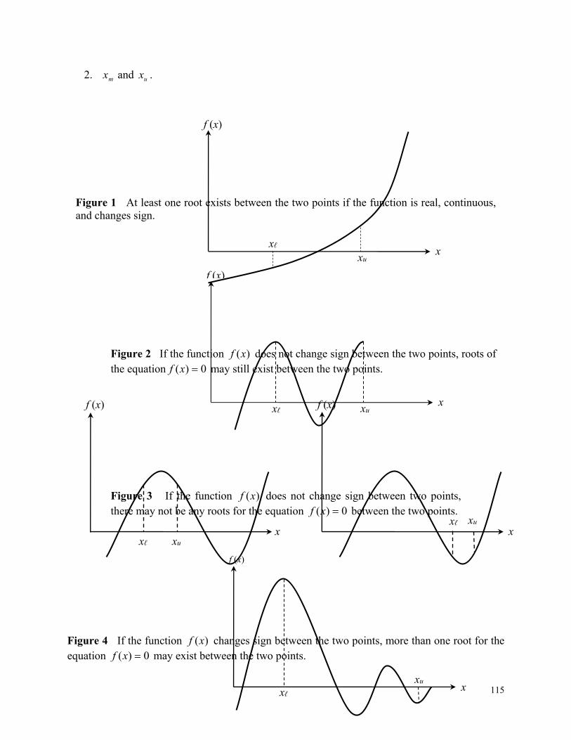
115

2. mx and ux .

Figure 1 At least one root exists between the two points if the function is real, continuous, and changes sign.

Figure 2 If the function )(xf does not change sign between the two points, roots of the equation 0)( xf may still exist between the two points.

Figure 3 If the function )(xf does not change sign between two points, there may not be any roots for the equation 0)( xf between the two points.

Figure 4 If the function )(xf changes sign between the two points, more than one root for the equation 0)( xf may exist between the two points.

f (x)

xℓ xu

x

f (x)

xℓ xu x

f (x)

xℓ xu

x

f (x)

xℓ xu x

f (x)

xℓ xu

x

116

Is the root now between x and mx or between mx and ux ? Well, one can find the sign of

)()( mxfxf , and if 0)()( mxfxf then the new bracket is between x and mx , otherwise, it is

between mx and ux . So, you can see that you are literally halving the interval. As one repeats

this process, the width of the interval uxx , becomes smaller and smaller, and you can zero in

to the root of the equation 0)( xf . The algorithm for the bisection method is given as follows.

Algorithm for the bisection method The steps to apply the bisection method to find the root of the equation 0)( xf are

1. Choose x and ux as two guesses for the root such that 0)()( uxfxf , or in other

words, )(xf changes sign between x and ux .

2. Estimate the root, mx , of the equation 0)( xf as the mid-point between x and ux as

2

= u

m

xxx

3. Now check the following a) If 0)()( mxfxf , then the root lies between x and mx ; then xx and mu xx .

b) If 0)()( mxfxf , then the root lies between mx and ux ; then mxx and uu xx .

c) If 0)()( mxfxf ; then the root is mx . Stop the algorithm if this is true.

4. Find the new estimate of the root

2

= u

m

xxx

Find the absolute relative approximate error as

100 -

= new

oldnew

m

mma x

xx

where new

mx = estimated root (tahmini kök) from present iteration (yinelemek)

oldmx = estimated root from previous iteration

5. Compare the absolute relative approximate error a with the pre-specified relative error

tolerance s . If sa , then go to Step 3, else stop the algorithm. Note one should

also check whether the number of iterations is more than the maximum number of iterations allowed. If so, one needs to terminate the algorithm and notify the user about it.

Example 1 You are working for ‘DOWN THE TOILET COMPANY’ that makes floats for ABC commodes (klozet). The floating ball has a specific gravity of 0.6 and has a radius of 5.5 cm. You are asked to find the depth to which the ball is submerged when floating in water.

The equation that gives the depth x to which the ball is submerged under water is given by

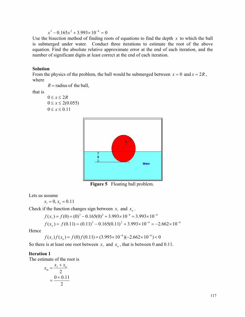
117

010993.3165.0 423 xx Use the bisection method of finding roots of equations to find the depth x to which the ball is submerged under water. Conduct three iterations to estimate the root of the above equation. Find the absolute relative approximate error at the end of each iteration, and the number of significant digits at least correct at the end of each iteration.

Solution From the physics of the problem, the ball would be submerged between 0x and Rx 2 , where

ball, theof radiusR that is

Rx 20 )055.0(20 x

11.00 x

Figure 5 Floating ball problem.

Lets us assume 11.0 ,0 uxx

Check if the function changes sign between x and ux . 4423 10993.310993.3)0(165.0)0()0()( fxf

4423 10662.210993.3)11.0(165.0)11.0()11.0()( fxf u

Hence 0)10662.2)(10993.3()11.0()0()()( 44 ffxfxf u

So there is at least one root between x and ux , that is between 0 and 0.11.

Iteration 1 The estimate of the root is

2u

m

xxx

2

11.00

118

055.0

5423 10655.610993.3055.0165.0055.0055.0 fxf m 010655.610993.3)055.0()0()()( 44 ffxfxf m

Hence the root is bracketed between mx and ux , that is, between 0.055 and 0.11. So, the lower

and upper limit of the new bracket is 11.0 ,055.0 uxx

At this point, the absolute relative approximate error a cannot be calculated as we do not have

a previous approximation.

Iteration 2 The estimate of the root is

2u

m

xxx

2

11.0055.0

0825.0 4423 10622.110993.3)0825.0(165.0)0825.0()0825.0()( fxf m

010622.110655.60825.0055.0 45 ffxfxf m

Hence, the root is bracketed between x and mx , that is, between 0.055 and 0.0825. So the

lower and upper limit of the new bracket is 0825.0 ,055.0 uxx

The absolute relative approximate error a at the end of Iteration 2 is

100new

oldnew

m

mma x

xx

1000825.0

055.00825.0

%33.33 None of the significant digits are at least correct in the estimated root of 0825.0mx because

the absolute relative approximate error is greater than 5%.

Iteration 3

2u

m

xxx

2

0825.0055.0

06875.0 5423 10563.510993.3)06875.0(165.0)06875.0()06875.0()( fxf m

0)105.563()10655.6()06875.0()055.0()()( 55 ffxfxf m

Hence, the root is bracketed between x and mx , that is, between 0.055 and 0.06875. So the

lower and upper limit of the new bracket is

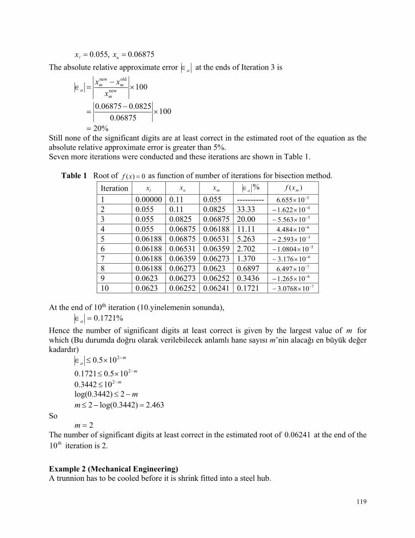
119

06875.0 ,055.0 uxx

The absolute relative approximate error a at the ends of Iteration 3 is

100new

oldnew

m

mma x

xx

10006875.0

0825.006875.0

%20 Still none of the significant digits are at least correct in the estimated root of the equation as the absolute relative approximate error is greater than 5%. Seven more iterations were conducted and these iterations are shown in Table 1. Table 1 Root of 0)( xf as function of number of iterations for bisection method.

Iteration x ux mx a % )( mxf

1 0.00000 0.11 0.055 ---------- 510655.6 2 0.055 0.11 0.0825 33.33 410622.1 3 0.055 0.0825 0.06875 20.00 510563.5 4 0.055 0.06875 0.06188 11.11 610484.4 5 0.06188 0.06875 0.06531 5.263 510593.2 6 0.06188 0.06531 0.06359 2.702 5100804.1 7 0.06188 0.06359 0.06273 1.370 610176.3 8 0.06188 0.06273 0.0623 0.6897 710497.6 9 0.0623 0.06273 0.06252 0.3436 610265.1 10 0.0623 0.06252 0.06241 0.1721 7100768.3

At the end of 10th iteration (10.yinelemenin sonunda),

%1721.0a

Hence the number of significant digits at least correct is given by the largest value of m for which (Bu durumda doğru olarak verilebilecek anlamlı hane sayısı m’nin alacağı en büyük değer kadardır)

ma

2105.0 m 2105.01721.0

m 2103442.0 m 2)3442.0log(

463.2)3442.0log(2 m So

2m The number of significant digits at least correct in the estimated root of 06241.0 at the end of the

th10 iteration is 2.

Example 2 (Mechanical Engineering) A trunnion has to be cooled before it is shrink fitted into a steel hub.

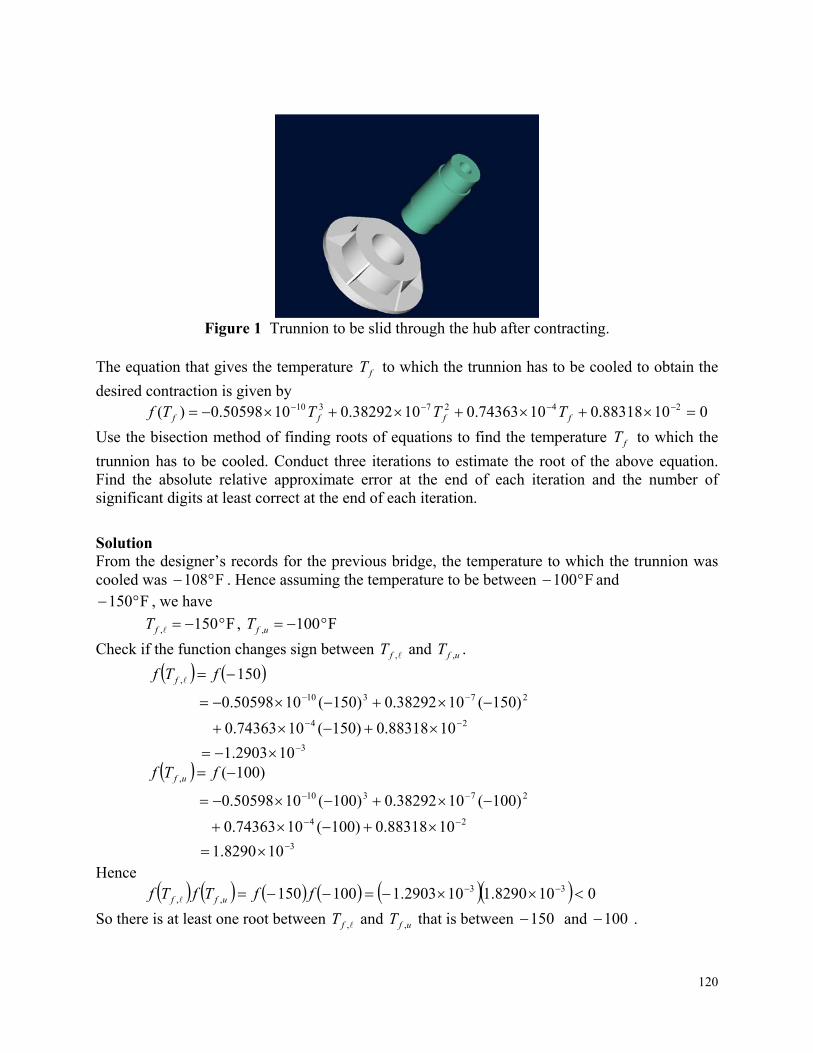
120

Figure 1 Trunnion to be slid through the hub after contracting.

The equation that gives the temperature fT to which the trunnion has to be cooled to obtain the

desired contraction is given by 010 88318.010 74363.010 38292.010 50598.0)( 2427310 T T T Tf ffff

Use the bisection method of finding roots of equations to find the temperature fT to which the

trunnion has to be cooled. Conduct three iterations to estimate the root of the above equation. Find the absolute relative approximate error at the end of each iteration and the number of significant digits at least correct at the end of each iteration.

Solution From the designer’s records for the previous bridge, the temperature to which the trunnion was cooled was F108 . Hence assuming the temperature to be between F100 and

F150 , we have

F150, fT , F100, ufT

Check if the function changes sign between ,fT and ufT , .

24

27310

,

10 88318.0)150(10 74363.0

)150(10 38292.0)150(10 50598.0

150

fTf f

310 2903.1

24

27310

,

10 88318.0)100(10 74363.0

)100(10 38292.0)100(10 50598.0

)100(

fTf uf

310 8290.1 Hence

010 8290.110 2903.1100150 33,, ffTfTf uff

So there is at least one root between ,fT and ufT , that is between 150 and 100 .

121

Iteration 1 The estimate of the root is

2,,

,uff

mf

TTT

2

)100(150

125

24

27310

,

10 88318.0)125(10 74363.0

)125(10 38292.0)125(10 50598.0

125

fTf mf

4102.3356 010 3356.210 2903.1125150 43

,, ffTfTf mff

Hence the root is bracketed between ,fT and mfT , , that is, between 150 and 125 .

So, the lower and upper limits of the new bracket are 125,150 ,, uff TT

At this point, the absolute relative approximate error a cannot be calculated, as we do not have

a previous approximation.

Iteration 2 The estimate of the root is

2,,

,uff

mf

TTT

2

125150

5.137

10 88318.0)5.137(10 74363.0

)5.137(10 38292.0)5.137(10 50598.0

5.137

24

27310

,

fTf mf

410 5.3762 = 010 3356.210 3762.51255.137 44

,, ffTfTf ufmf

Hence, the root is bracketed between mfT , and ufT , , that is, between 125 and 5.137 .

So the lower and upper limits of the new bracket are 125,5.137 ,, uff TT

The absolute relative approximate error a at the end of Iteration 2 is

100new,

old,

new,

mf

mfmfa T

TT

122

1005.137

)125(5.137

%0909.9 None of the significant digits are at least correct in the estimated root of

5.137, mfT

as the absolute relative approximate error is greater that %5 .

Iteration 3 The estimate of the root is

2,,

,uff

mf

TTT

2

)125(5.137

25.131

10 88318.0)25.131(10 74363.0

)25.131(10 38292.0)25.131(10 50598.0

25.131

24

27310

,

fTf mf

410 1.54303 = 010 5430.110 3356.225.131125 44

,, ffTfTf mff

Hence, the root is bracketed between ,fT and mfT , , that is, between 125 and 25.131 .

So the lower and upper limits of the new bracket are 125,25.131 ,, uff TT

The absolute relative approximate error a at the ends of Iteration 3 is

100new,

old,

new,

mf

mfmfa T

TT

10025.131

)5.137(25.131

%7619.4 The number of significant digits at least correct is 1. Seven more iterations were conducted and these iterations are shown in the Table 1 below.

Table 1 Root of 0xf as function of number of iterations for bisection method.

123

Iteration ,fT ufT , mfT , %a mfTf ,

1 2 3 4 5 6 7 8 9 10

−150 −150 −137.5 −131.25 −131.25 −129.69 −128.91 −128.91 −128.91 −128.81

−100 −125 −125 −125 −128.13 −123.13 −123.13 −128.52 −128.71 −128.71

−125 −137.5 −131.25 −128.13 −129.69 −128.91 −128.52 −128.71 −128.81 −128.76

--------- 9.0909 4.7619 2.4390 1.2048 0.60606 0.30395 0.15175 0.075815 0.037922

4102.3356 4105.3762 4101.5430

5103.9065 5105.7760 6109.3826

5101.4838 6102.7228

6103.3305 7103.0396

At the end of the th10 iteration, %037922.0a

Hence, the number of significant digits at least correct is given by the largest value of m for which m

a 2105.0

m 2105.0037922.0 m 210075844.0 m 2075844.0log

1201.3075844.0log2 m So

3m The number of significant digits at least correct in the estimated root of 76.128 is 3.

Example 3 (Industrial Engineering) You are working for a start-up computer assembly company and have been asked to determine the minimum number of computers that the shop will have to sell to make a profit. The equation that gives the minimum number of computers n to be sold after considering the total costs and the total sales is

03500087540)( 5.1 nnnf Use the bisection method of finding roots of equations to find the minimum number of computers that need to be sold to make a profit. Conduct three iterations to estimate the root of the above equation. Find the absolute relative approximate error at the end of each iteration and the number of significant digits at least correct at the end of each iteration.

Solution Let us assume 100,50 unn

Check if the function changes sign between n and un .

124

1.539235000)50(875)50(4050)( 5.1 fnf

1250035000)100(875)100(40)100() 5.1 ff(nu

Hence 0125001.539210050 ffnfnf u

So there is at least one root between n and un , that is, between 50 and 100.

Iteration 1 The estimate of the root is

2u

m

nnn

2

10050

75 35.1 10 6442.435000)75(875)75(4075 fnf m

010 6442.41.53927550 3 ffnfnf m

Hence the root is bracketed between n and mn , that is, between 50 and 75. So, the lower and

upper limits of the new bracket are 75,50 unn

At this point, the absolute relative approximate error a cannot be calculated, as we do not have

a previous approximation.

Iteration 2 The estimate of the root is

2u

m

nnn

2

7550

5.62 735.7635000)5.62(875)5.62(405.62 5.1 fnf m

0735.761.53925.6250 ffnfnf m

Hence, the root is bracketed between mn and un , that is, between 62.5 and 75. So the lower and

upper limits of the new bracket are 75,5.62 unn

The absolute relative approximate error, a at the end of Iteration 2 is

100new

oldnew

m

mma n

nn

1005.62

755.62

%20 None of the significant digits are at least correct in the estimated root

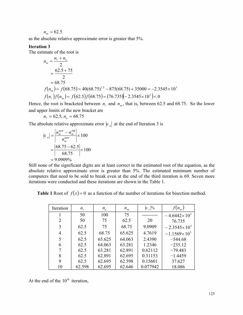
125

5.62mn

as the absolute relative approximate error is greater that 5%.

Iteration 3 The estimate of the root is

2u

m

nnn

2

755.62

75.68 35.1 10 3545.235000)75.68(875)75.68(4075.68 fnf m

010 3545.2735.7675.685.62 3 ffnfnf m

Hence, the root is bracketed between n and mn , that is, between 62.5 and 68.75. So the lower

and upper limits of the new bracket are 75.68,5.62 unn

The absolute relative approximate error a at the end of Iteration 3 is

100new

oldnew

m

mma n

nn

10075.68

5.6275.68

%0909.9 Still none of the significant digits are at least correct in the estimated root of the equation, as the absolute relative approximate error is greater than 5%. The estimated minimum number of computers that need to be sold to break even at the end of the third iteration is 69. Seven more iterations were conducted and these iterations are shown in the Table 1.

Table 1 Root of 0xf as a function of the number of iterations for bisection method.

Iteration n un mn %a mnf

1 2 3 4 5 6 7 8 9 10

50 50

62.5 62.5 62.5 62.5 62.5 62.5 62.5

62.598

100 75 75

68.75 65.625 64.063 63.281 62.891 62.695 62.695

75 62.5 68.75 65.625 64.063 63.281 62.891 62.695 62.598 62.646

---------- 20

9.0909 4.7619 2.4390 1.2346 0.62112 0.31153 0.15601 0.077942

3104.6442 76.735

3102.3545 3101.1569

−544.68 −235.12 −79.483 −1.4459 37.627 18.086

At the end of the th10 iteration,

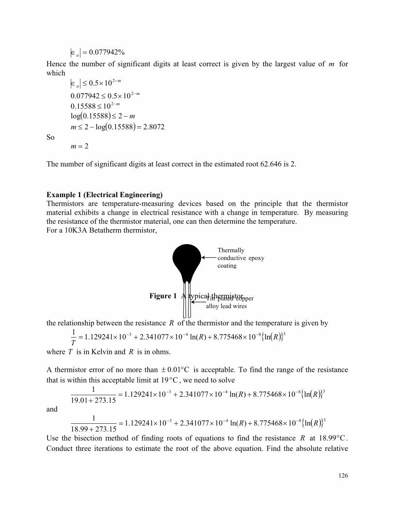
126

%077942.0a

Hence the number of significant digits at least correct is given by the largest value of m for which m

a 2105.0

m 2105.0077942.0 m 21015588.0 m 215588.0log

8072.215588.0log2 m So

2m

The number of significant digits at least correct in the estimated root 62.646 is 2.

Example 1 (Electrical Engineering) Thermistors are temperature-measuring devices based on the principle that the thermistor material exhibits a change in electrical resistance with a change in temperature. By measuring the resistance of the thermistor material, one can then determine the temperature. For a 10K3A Betatherm thermistor,

Figure 1 A typical thermistor. the relationship between the resistance R of the thermistor and the temperature is given by

3843 ln10775468.8)ln(10341077.210129241.11

RRT

where T is in Kelvin and R is in ohms. A thermistor error of no more than C01.0 is acceptable. To find the range of the resistance that is within this acceptable limit at C 19 , we need to solve

3843 ln10775468.8)ln(10341077.210129241.115.27301.19

1RR

and

3843 ln10775468.8)ln(10341077.210129241.115.27399.18

1RR

Use the bisection method of finding roots of equations to find the resistance R at C99.18 . Conduct three iterations to estimate the root of the above equation. Find the absolute relative

Thermally conductive epoxy coating

Tin plated copper alloy lead wires

127

approximate error at the end of each iteration and the number of significant digits at least correct at the end of each iteration.

Solution Solving

3843 ln10775468.8)ln(10341077.210129241.115.27399.18

1RR

we get

3384 10293775.2ln10775468.8)ln(10341077.2)( RRRf Lets us assume 14000,11000 uRR

Check if the function changes sign between R and uR .

5

3384

104536.4

10293775.211000ln10775468.8)11000ln(10341077.2

)11000()(

fRf

5

3384

107563.1

10293775.214000ln10775468.8)14000ln(10341077.2

)14000()(

fRf u

Hence 0107563.1104536.41400011000 55 ffRfRf u

So there is at least one root between R and uR , that is, between 11000 and 14000 .

Iteration 1 The estimate of the root is

2u

m

RRR

2

1400011000

12500

5

3384

101655.1

10293775.212500ln10775468.8)12500ln(10341077.2

)12500()(

fRf m

0101655.1104536.41250011000 55 ffRfRf m

Hence the root is bracketed between mR and uR , that is, between 12500 and 14000 . So, the

lower and upper limits of the new bracket are 14000,12500 uRR

128

At this point, the absolute relative approximate error a cannot be calculated as we do not have

a previous approximation.

Iteration 2 The estimate of the root is

2u

m

RRR

2

1400012500

13250

6

3384

103599.3

10293775.213250ln10775468.813250ln10341077.2

13250

fRf m

0103599.3101655.11325012500 65 ffRfRf m

Hence, the root is bracketed between R and mR , that is, between 12500 and 13250 .

So the lower and upper limits of the new bracket are 13250,12500 uRR

The absolute relative approximate error a at the end of Iteration 2 is

100new

oldnew

m

mma R

RR

10013250

1250013250

%6604.5 None of the significant digits are at least correct in the estimated root 13250mR

as the absolute relative approximate error is greater than %5 .

Iteration 3

2u

m

RRR

2

1325012500

12875

6

3384

100403.4

10293775.212875ln10775468.812875ln10341077.2

12875

fRf m

0100398.4101654.11287512500 65 ffRfRf m

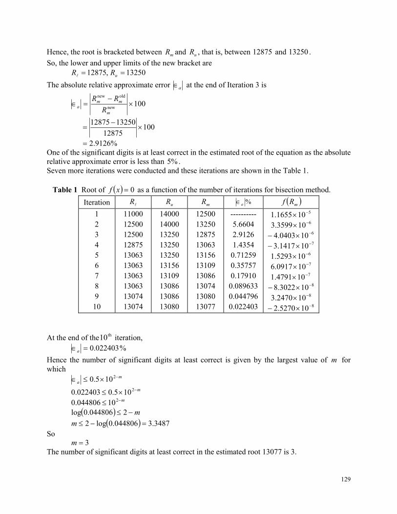
129

Hence, the root is bracketed between mR and uR , that is, between 12875 and 13250 .

So, the lower and upper limits of the new bracket are 13250,12875 uRR

The absolute relative approximate error a at the end of Iteration 3 is

100new

oldnew

m

mma R

RR

10012875

1325012875

%9126.2 One of the significant digits is at least correct in the estimated root of the equation as the absolute relative approximate error is less than %5 . Seven more iterations were conducted and these iterations are shown in the Table 1.

Table 1 Root of 0xf as a function of the number of iterations for bisection method.

Iteration R uR mR %a mRf

1 2 3 4 5 6 7 8 9 10

11000 12500 12500 12875 13063 13063 13063 13063 13074 13074

14000 14000 13250 13250 13250 13156 13109 13086 13086 13080

12500 13250 12875 13063 13156 13109 13086 13074 13080 13077

---------- 5.6604 2.9126 1.4354 0.71259 0.35757 0.17910 0.089633 0.044796 0.022403

5101.1655 6103.3599

6104.0403 7103.1417

6101.5293 7106.0917 7101.4791

8108.3022 8103.2470

8102.5270

At the end of the th10 iteration, %022403.0a

Hence the number of significant digits at least correct is given by the largest value of m for which m

a 2105.0

m 2105.0022403.0 m 210044806.0 m 2044806.0log

3487.3044806.0log2 m So

3m The number of significant digits at least correct in the estimated root 13077 is 3.

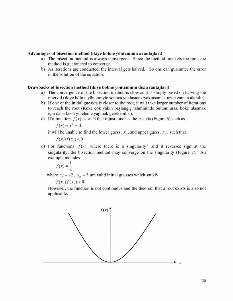
130

Advantages of bisection method (ikiye bölme yönteminin avantajları) a) The bisection method is always convergent. Since the method brackets the root, the

method is guaranteed to converge. b) As iterations are conducted, the interval gets halved. So one can guarantee the error

in the solution of the equation.

Drawbacks of bisection method (ikiye bölme yönteminin dez avantajları) a) The convergence of the bisection method is slow as it is simply based on halving the

interval (ikiye bölme yöntemiyle sonuca yaklaşmak/yakınsamak uzun zaman alabilir). b) If one of the initial guesses is closer to the root, it will take larger number of iterations

to reach the root (Köke çok yakın başlangıç tahmininde bulunulursa, köke ulaşmak için daha fazla yineleme yapmak gerekebilir ).

c) If a function )(xf is such that it just touches the x -axis (Figure 6) such as

0)( 2 xxf

it will be unable to find the lower guess, x , and upper guess, ux , such that

0)()( uxfxf

d) For functions )(xf where there is a singularity1 and it reverses sign at the singularity, the bisection method may converge on the singularity (Figure 7). An example includes

xxf

1)(

where 2x , 3ux are valid initial guesses which satisfy

0)()( uxfxf

However, the function is not continuous and the theorem that a root exists is also not applicable.

f (x)

x

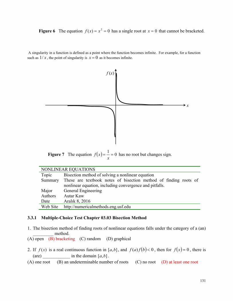
131

Figure 6 The equation 0)( 2 xxf has a single root at 0x that cannot be bracketed. A singularity in a function is defined as a point where the function becomes infinite. For example, for a function such as x/1 , the point of singularity is 0x as it becomes infinite.

Figure 7 The equation 01

xxf has no root but changes sign.

NONLINEAR EQUATIONS Topic Bisection method of solving a nonlinear equation Summary These are textbook notes of bisection method of finding roots of

nonlinear equation, including convergence and pitfalls. Major General Engineering Authors Autar Kaw Date Aralık 8, 2016 Web Site http://numericalmethods.eng.usf.edu

3.3.1 Multiple-Choice Test Chapter 03.03 Bisection Method 1. The bisection method of finding roots of nonlinear equations falls under the category of a (an)

_________ method. (A) open (B) bracketing (C) random (D) graphical 2. If )(xf is a real continuous function in ],[ ba , and 0)( bfaf , then for 0xf , there is

(are) ____________ in the domain ],[ ba . (A) one root (B) an undeterminable number of roots (C) no root (D) at least one root

f (x)

x

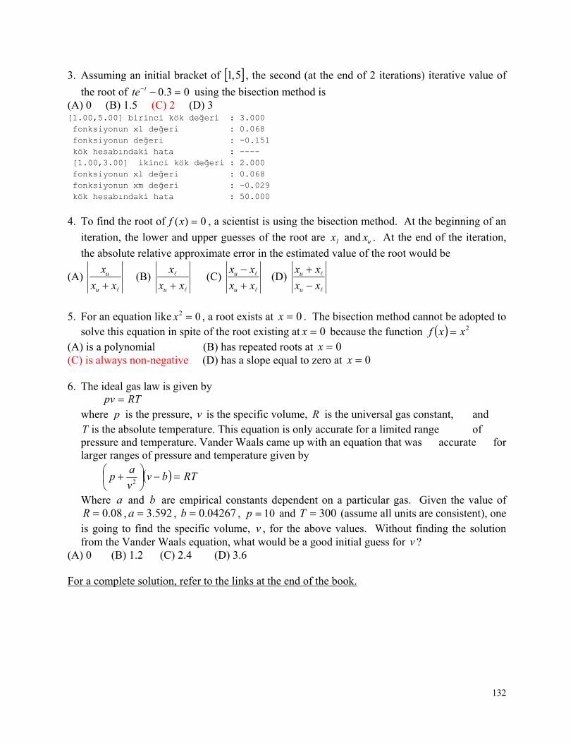
132

3. Assuming an initial bracket of 5,1 , the second (at the end of 2 iterations) iterative value of

the root of 03.0 tte using the bisection method is (A) 0 (B) 1.5 (C) 2 (D) 3 [1.00,5.00] birinci kök değeri : 3.000 fonksiyonun xl değeri : 0.068 fonksiyonun değeri : -0.151 kök hesabındaki hata : ---- [1.00,3.00] ikinci kök değeri : 2.000 fonksiyonun xl değeri : 0.068 fonksiyonun xm değeri : -0.029 kök hesabındaki hata : 50.000

4. To find the root of 0)( xf , a scientist is using the bisection method. At the beginning of an

iteration, the lower and upper guesses of the root are lx and ux . At the end of the iteration,

the absolute relative approximate error in the estimated value of the root would be

(A) xx

x

u

u

(B)

xx

x

u (C)

xx

xx

u

u

(D)

xx

xx

u

u

5. For an equation like 02 x , a root exists at 0x . The bisection method cannot be adopted to

solve this equation in spite of the root existing at 0x because the function 2xxf (A) is a polynomial (B) has repeated roots at 0x (C) is always non-negative (D) has a slope equal to zero at 0x 6. The ideal gas law is given by RTpv where p is the pressure, v is the specific volume, R is the universal gas constant, and

T is the absolute temperature. This equation is only accurate for a limited range of pressure and temperature. Vander Waals came up with an equation that was accurate for larger ranges of pressure and temperature given by

RTbvv

ap

2

Where a and b are empirical constants dependent on a particular gas. Given the value of 08.0R , 592.3a , 04267.0b , 10p and 300T (assume all units are consistent), one

is going to find the specific volume, v , for the above values. Without finding the solution from the Vander Waals equation, what would be a good initial guess for v ?

(A) 0 (B) 1.2 (C) 2.4 (D) 3.6 For a complete solution, refer to the links at the end of the book.

133

3.4 Chapter 03.04 Newton-Raphson Method of Solving a Nonlinear Equation

PRE-REQUISITES

1. Know the definition of a derivative of a function (Primer for Differential Calculus). 2. Be able to find derivatives of function (Primer for Differential Calculus). 3. Know what a tangent to a curve is and how to find the tangent line (Primer for

Differential Calculus).

OBJECTIVES

1. derive the Newton-Raphson method formula, 2. develop the algorithm of the Newton-Raphson method, 3. use the Newton-Raphson method to solve a nonlinear equation, and 4. discuss the drawbacks of the Newton-Raphson method.

After reading this chapter, you should be able to:

1. derive the Newton-Raphson method formula, 2. develop the algorithm of the Newton-Raphson method, 3. use the Newton-Raphson method to solve a nonlinear equation, and 4. discuss the drawbacks of the Newton-Raphson method.

Introduction Methods such as the bisection method and the false position method of finding roots of a nonlinear equation 0)( xf require bracketing of the root by two guesses (f(x)=0 şeklindeki çizgisel olmayan bir eşitliğin bisection ve false position gibi yöntemlerde çözüm aralığının tahmin edilmesi gerekmektedir). Such methods are called bracketing methods (aralık yöntemi). These methods are always convergent since they are based on reducing the interval between the two guesses so as to zero in on the root of the equation (eşitliği sıfıra yaklaştıracak aralığı daralttıkça bu yöntemlerle bir sonuca ulaşılabilir).

In the Newton-Raphson method, the root is not bracketed (Newton-Raphson yönteminde kök bölgesi yoktur). In fact, only one initial guess of the root is needed to get the iterative process started to find the root of an equation (aslında bir başlangıç tahmini kök değeri yinelemeyi başlatmak için yeterli olacaktır). The method hence falls in the category of open methods (yöntem açık yöntem kategorisine alınabilir). Convergence in open methods is not guaranteed but if the method does converge, it does so much faster than the bracketing methods.

Derivation The Newton-Raphson method is based on the principle that if the initial guess of the root of

0)( xf is at ix , then if one draws the tangent to the curve at )( ixf , the point 1ix where the

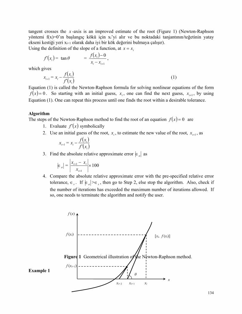
134

tangent crosses the x -axis is an improved estimate of the root (Figure 1) (Newton-Raphson yöntemi f(x)=0’ın başlangıç kökü için xi’yi alır ve bu noktadaki tanjantının/teğetinin yatay ekseni kestiği yeri xi+1 olarak daha iyi bir kök değerini bulmaya çalışır). Using the definition of the slope of a function, at ixx

θ = xf i tan 1

0

ii

i

xx

xf = ,

which gives i

iii xf

xf = xx

1 (1)

Equation (1) is called the Newton-Raphson formula for solving nonlinear equations of the form 0xf . So starting with an initial guess, ix , one can find the next guess, 1ix , by using

Equation (1). One can repeat this process until one finds the root within a desirable tolerance.

Algorithm The steps of the Newton-Raphson method to find the root of an equation 0xf are

1. Evaluate xf symbolically

2. Use an initial guess of the root, ix , to estimate the new value of the root, 1ix , as

i

iii xf

xf = xx

1

3. Find the absolute relative approximate error a as

0101

1

i

iia x

xx =

4. Compare the absolute relative approximate error with the pre-specified relative error tolerance, s . If a > s , then go to Step 2, else stop the algorithm. Also, check if

the number of iterations has exceeded the maximum number of iterations allowed. If so, one needs to terminate the algorithm and notify the user.

Figure 1 Geometrical illustration of the Newton-Raphson method.

Example 1

f (x)

f (xi)

f (xi+1)

xi+2 xi+1 xi x

θ

[xi, f (xi)]

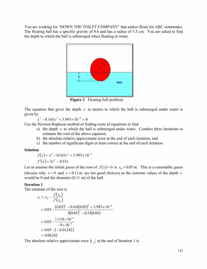
135

You are working for ‘DOWN THE TOILET COMPANY’ that makes floats for ABC commodes. The floating ball has a specific gravity of 0.6 and has a radius of 5.5 cm. You are asked to find the depth to which the ball is submerged when floating in water.

Figure 2 Floating ball problem.

The equation that gives the depth x in meters to which the ball is submerged under water is given by

010993.3165.0 423 xx Use the Newton-Raphson method of finding roots of equations to find

a) the depth x to which the ball is submerged under water. Conduct three iterations to estimate the root of the above equation.

b) the absolute relative approximate error at the end of each iteration, and c) the number of significant digits at least correct at the end of each iteration.

Solution 423 10993.31650 x.xxf

x.xxf 3303 2

Let us assume the initial guess of the root of 0xf is ..x m 0500 This is a reasonable guess

(discuss why 0x and m 11.0x are not good choices) as the extreme values of the depth x would be 0 and the diameter (0.11 m) of the ball.

Iteration 1 The estimate of the root is

0

001 xf

xfxx

0503300503

10993.30501650050050

2

423

...

....

3

4

109

10118.1050

.

01242.0050 . 062420. The absolute relative approximate error a at the end of Iteration 1 is

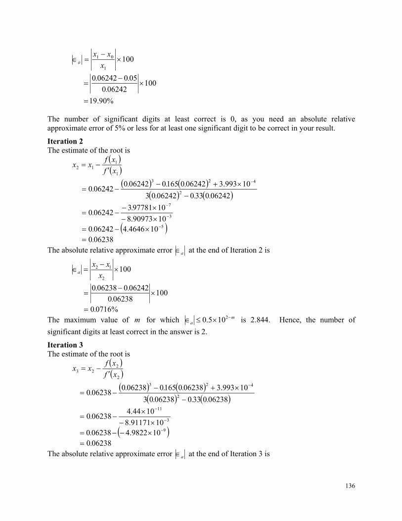
136

1001

01

x

xxa

19.90%

100062420

050062420

.

..

The number of significant digits at least correct is 0, as you need an absolute relative approximate error of 5% or less for at least one significant digit to be correct in your result.

Iteration 2 The estimate of the root is

1

112 xf

xfxx

0624203300624203

10993.30624201650062420062420

2

423

...

....

3

7

1090973.8

10977813062420

.

.

5104646.4062420 . 062380.

The absolute relative approximate error a at the end of Iteration 2 is

1002

12

x

xxa

100062380

062420062380

.

..

%07160. The maximum value of m for which m

a 2105.0 is 2.844. Hence, the number of

significant digits at least correct in the answer is 2.

Iteration 3 The estimate of the root is

2

223 xf

xfxx

0623803300623803

10993.30623801650062380062380

2

423

...

....

3

11

1091171.8

1044.4062380

.

9109822.4062380 . 062380. The absolute relative approximate error a at the end of Iteration 3 is

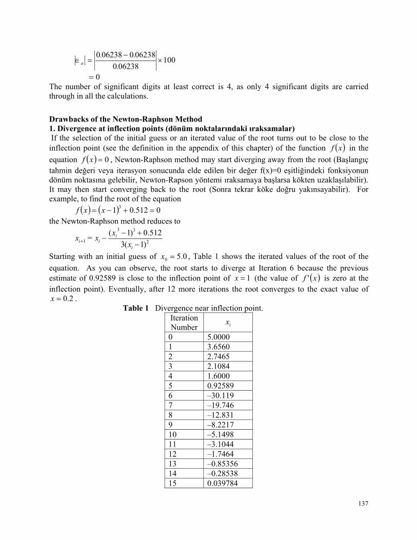
137

100062380

062380062380

.

..a

0 The number of significant digits at least correct is 4, as only 4 significant digits are carried through in all the calculations.

Drawbacks of the Newton-Raphson Method 1. Divergence at inflection points (dönüm noktalarındaki ıraksamalar) If the selection of the initial guess or an iterated value of the root turns out to be close to the inflection point (see the definition in the appendix of this chapter) of the function xf in the

equation 0xf , Newton-Raphson method may start diverging away from the root (Başlangıç tahmin değeri veya iterasyon sonucunda elde edilen bir değer f(x)=0 eşitliğindeki fonksiyonun dönüm noktasına gelebilir, Newton-Rapson yöntemi ıraksamaya başlarsa kökten uzaklaşılabilir). It may then start converging back to the root (Sonra tekrar köke doğru yakınsayabilir). For example, to find the root of the equation

0512.01 3 xxf the Newton-Raphson method reduces to

2

33

1 )1(3

512.0)1(

i

iii x

x = xx

Starting with an initial guess of 0.50 x , Table 1 shows the iterated values of the root of the

equation. As you can observe, the root starts to diverge at Iteration 6 because the previous estimate of 0.92589 is close to the inflection point of 1x (the value of xf ' is zero at the inflection point). Eventually, after 12 more iterations the root converges to the exact value of

2.0x . Table 1 Divergence near inflection point.

Iteration Number ix

0 5.0000 1 3.6560 2 2.7465 3 2.1084 4 1.6000 5 0.92589 6 –30.119 7 –19.746 8 –12.831 9 –8.2217 10 –5.1498 11 –3.1044 12 –1.7464 13 –0.85356 14 –0.28538 15 0.039784

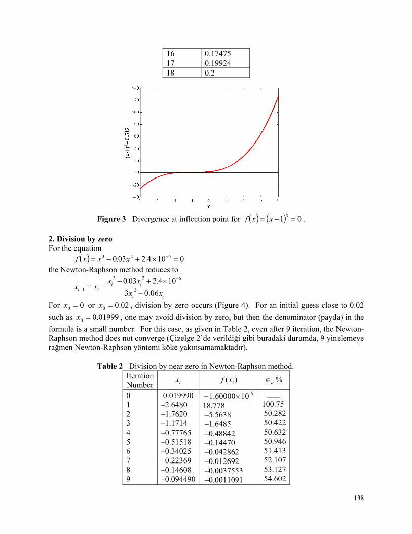
138

16 0.17475 17 0.19924 18 0.2

Figure 3 Divergence at inflection point for 01 3 xxf .

2. Division by zero For the equation

01042030 623 .x.xxf the Newton-Raphson method reduces to

ii

iiii

xx

.x.x = xx

06.03

10420302

623

1

For 00 x or 02.00 x , division by zero occurs (Figure 4). For an initial guess close to 0.02

such as 01999.00 x , one may avoid division by zero, but then the denominator (payda) in the

formula is a small number. For this case, as given in Table 2, even after 9 iteration, the Newton-Raphson method does not converge (Çizelge 2’de verildiği gibi buradaki durumda, 9 yinelemeye rağmen Newton-Raphson yöntemi köke yakınsamamaktadır).

Table 2 Division by near zero in Newton-Raphson method. Iteration Number ix )( ixf %a

0 1 2 3 4 5 6 7 8 9

0.019990 –2.6480 –1.7620 –1.1714 –0.77765 –0.51518 –0.34025 –0.22369 –0.14608 –0.094490

-6101.60000 18.778 –5.5638 –1.6485 –0.48842 –0.14470 –0.042862 –0.012692 –0.0037553 –0.0011091

100.75 50.282 50.422 50.632 50.946 51.413 52.107 53.127 54.602

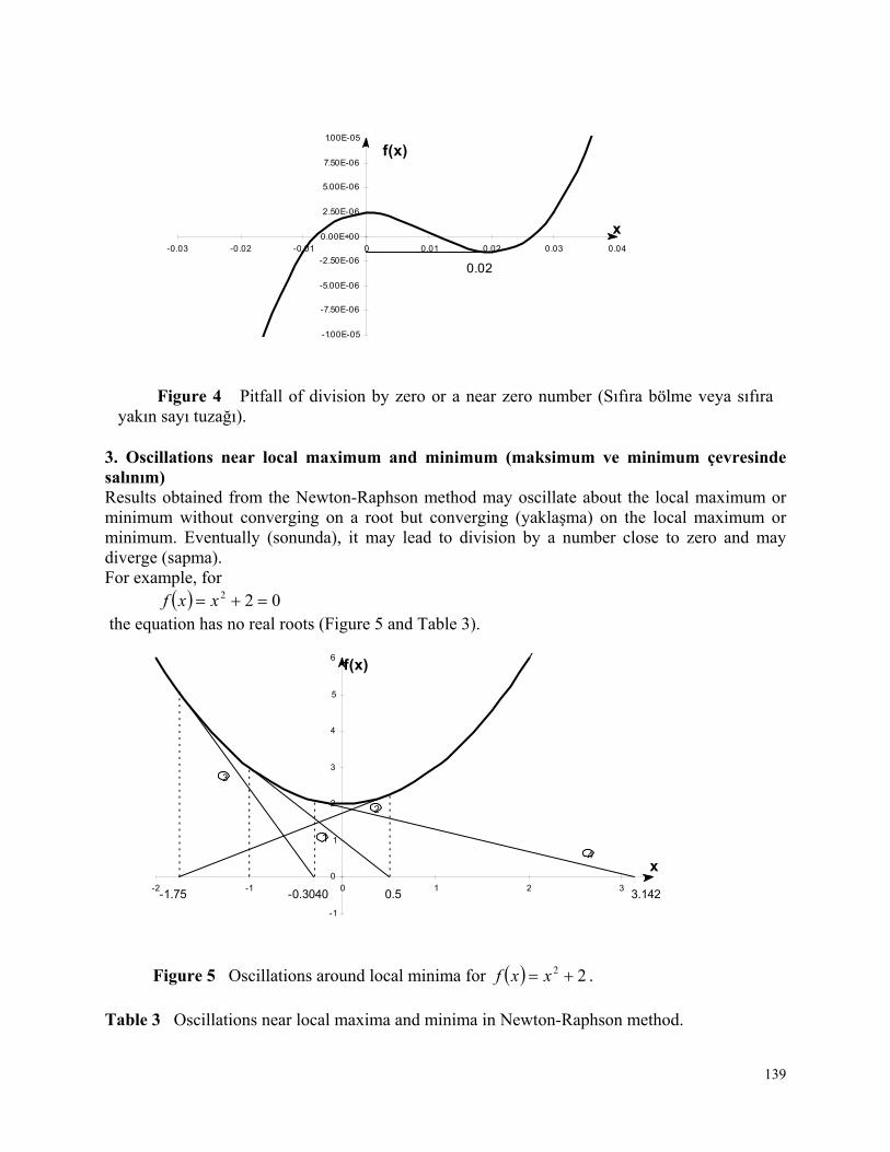
139

-1.00E-05

-7.50E-06

-5.00E-06

-2.50E-06

0.00E+00

2.50E-06

5.00E-06

7.50E-06

1.00E-05

-0.03 -0.02 -0.01 0 0.01 0.02 0.03 0.04

x

f(x)

0.02

Figure 4 Pitfall of division by zero or a near zero number (Sıfıra bölme veya sıfıra yakın sayı tuzağı).

3. Oscillations near local maximum and minimum (maksimum ve minimum çevresinde salınım) Results obtained from the Newton-Raphson method may oscillate about the local maximum or minimum without converging on a root but converging (yaklaşma) on the local maximum or minimum. Eventually (sonunda), it may lead to division by a number close to zero and may diverge (sapma). For example, for

022 xxf the equation has no real roots (Figure 5 and Table 3).

-1

0

1

2

3

4

5

6

-2 -1 0 1 2 3

f(x)

x

3

4

2

1

-1.75 -0.3040 0.5 3.142

Figure 5 Oscillations around local minima for 22 xxf .

Table 3 Oscillations near local maxima and minima in Newton-Raphson method.

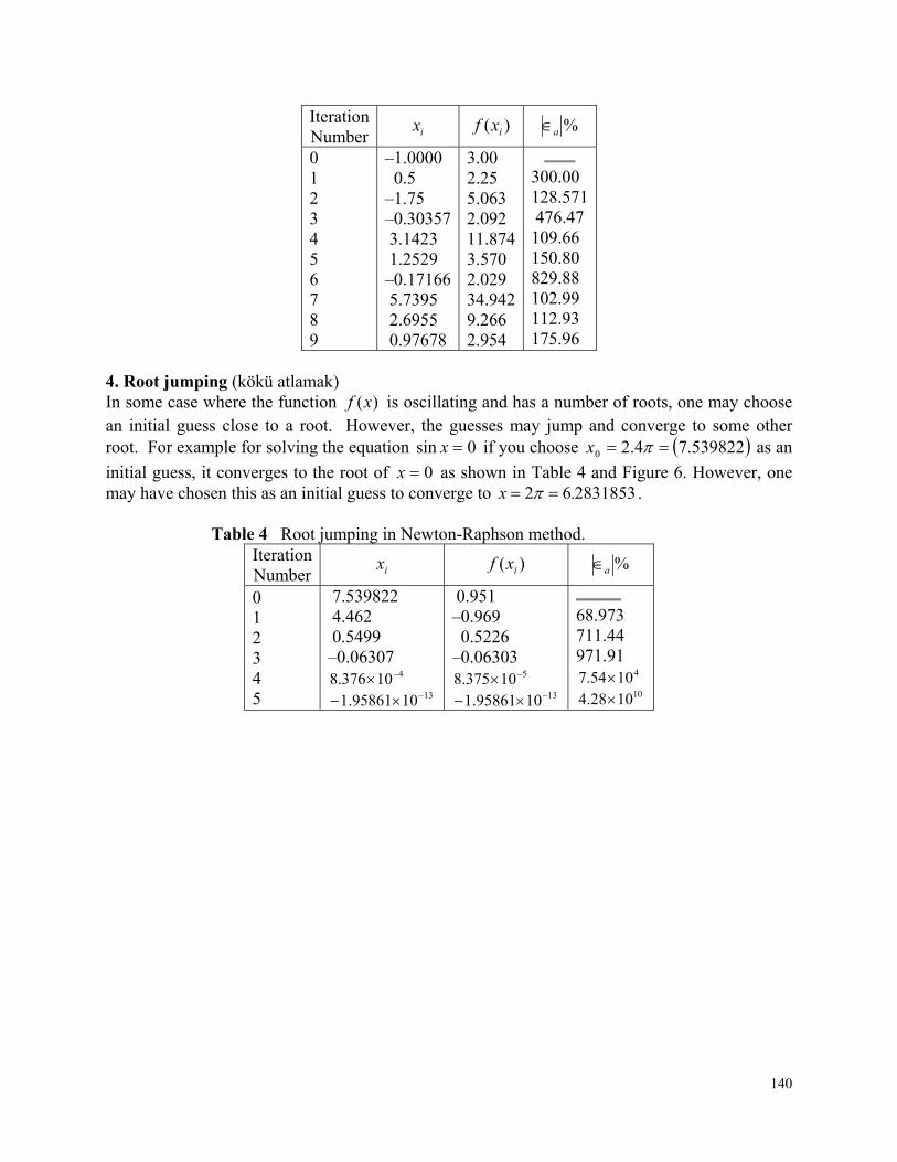
140

Iteration Number ix )( ixf %a

0 1 2 3 4 5 6 7 8 9

–1.0000 0.5 –1.75 –0.30357 3.1423 1.2529 –0.17166 5.7395 2.6955 0.97678

3.00 2.25 5.063 2.092 11.874 3.570 2.029 34.942 9.266 2.954

300.00 128.571 476.47 109.66 150.80 829.88 102.99 112.93 175.96

4. Root jumping (kökü atlamak) In some case where the function )(xf is oscillating and has a number of roots, one may choose an initial guess close to a root. However, the guesses may jump and converge to some other root. For example for solving the equation 0sin x if you choose 539822.74.20 x as an

initial guess, it converges to the root of 0x as shown in Table 4 and Figure 6. However, one may have chosen this as an initial guess to converge to 283185362 .x . Table 4 Root jumping in Newton-Raphson method.

Iteration Number ix )( ixf %a

0 1 2 3 4 5

7.539822 4.462 0.5499 –0.06307

410376.8 131095861.1

0.951 –0.969 0.5226 –0.06303

510375.8 131095861.1

68.973 711.44 971.91

41054.7 101028.4

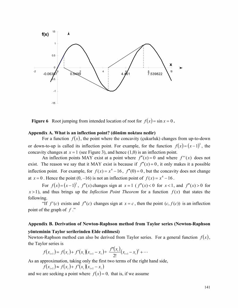
141

-1.5

-1

-0.5

0

0.5

1

1.5

-2 0 2 4 6 8 10

x

f(x)

-0.06307 0.5499 4.461 7.539822

Figure 6 Root jumping from intended location of root for 0sin xxf .

Appendix A. What is an inflection point? (dönüm noktası nedir)

For a function xf , the point where the concavity (çukurluk) changes from up-to-down

or down-to-up is called its inflection point. For example, for the function 31 xxf , the concavity changes at 1x (see Figure 3), and hence (1,0) is an inflection point.

An inflection points MAY exist at a point where 0)( xf and where )('' xf does not exist. The reason we say that it MAY exist is because if 0)( xf , it only makes it a possible

inflection point. For example, for 16)( 4 xxf , 0)0( f , but the concavity does not change

at 0x . Hence the point (0, –16) is not an inflection point of 16)( 4 xxf .

For 31 xxf , )(xf changes sign at 1x ( 0)( xf for 1x , and 0)( xf for 1x ), and thus brings up the Inflection Point Theorem for a function )(xf that states the

following. “If )(' cf exists and )(cf changes sign at cx , then the point ))(,( cfc is an inflection

point of the graph of f .”

Appendix B. Derivation of Newton-Raphson method from Taylor series (Newton-Raphson

yönteminin Taylor serilerinden Elde edilmesi) Newton-Raphson method can also be derived from Taylor series. For a general function xf , the Taylor series is

iiiii xxxfxfxf 11 +

21!2 ii

i xxxf"

As an approximation, taking only the first two terms of the right hand side, iiiii xxxfxfxf 11

and we are seeking a point where ,xf 0 that is, if we assume

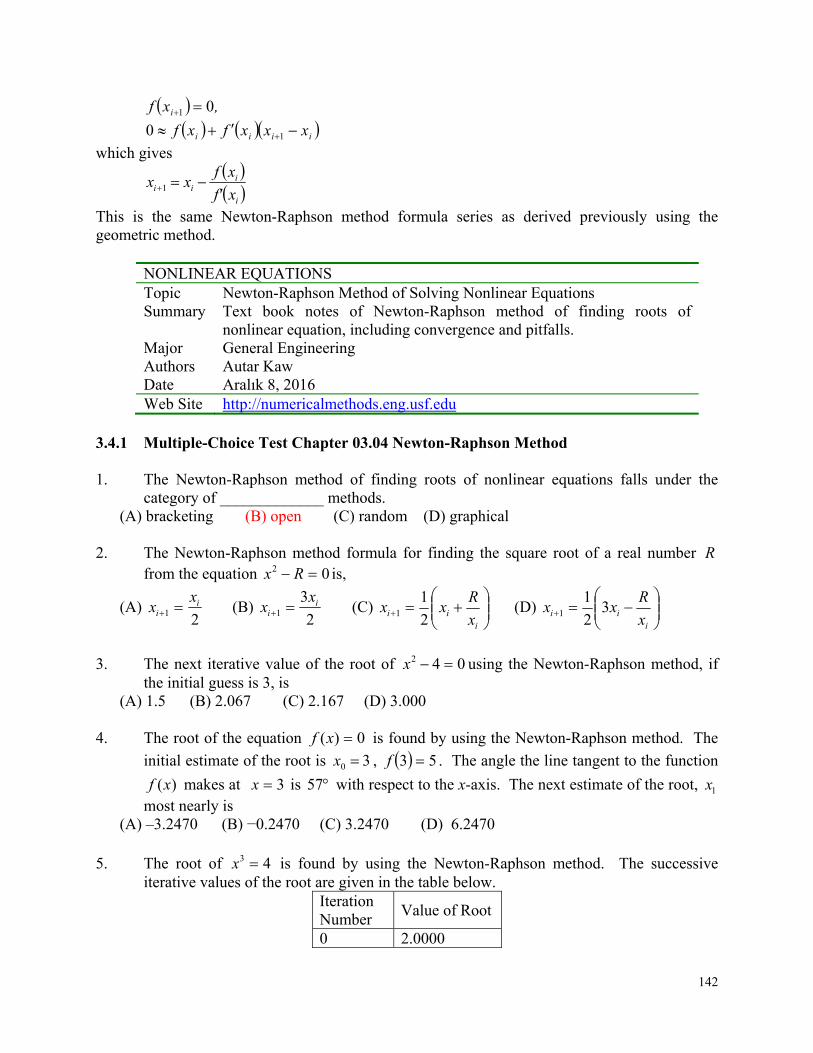
142

,xf i 01

iiii xxxfxf 10

which gives i

iii xf'

xfxx 1

This is the same Newton-Raphson method formula series as derived previously using the geometric method.

NONLINEAR EQUATIONS Topic Newton-Raphson Method of Solving Nonlinear Equations Summary Text book notes of Newton-Raphson method of finding roots of

nonlinear equation, including convergence and pitfalls. Major General Engineering Authors Autar Kaw Date Aralık 8, 2016 Web Site http://numericalmethods.eng.usf.edu

3.4.1 Multiple-Choice Test Chapter 03.04 Newton-Raphson Method 1. The Newton-Raphson method of finding roots of nonlinear equations falls under the

category of _____________ methods. (A) bracketing (B) open (C) random (D) graphical

2. The Newton-Raphson method formula for finding the square root of a real number R

from the equation 02 Rx is,

(A) 21

ii

xx (B)

2

31

ii

xx (C)

iii x

Rxx

2

11 (D)

iii x

Rxx 3

2

11

3. The next iterative value of the root of 042 x using the Newton-Raphson method, if

the initial guess is 3, is (A) 1.5 (B) 2.067 (C) 2.167 (D) 3.000

4. The root of the equation 0)( xf is found by using the Newton-Raphson method. The

initial estimate of the root is 30 x , 53 f . The angle the line tangent to the function

)(xf makes at 3x is 57 with respect to the x-axis. The next estimate of the root, 1x most nearly is

(A) –3.2470 (B) −0.2470 (C) 3.2470 (D) 6.2470 5. The root of 43 x is found by using the Newton-Raphson method. The successive

iterative values of the root are given in the table below. Iteration Number

Value of Root

0 2.0000

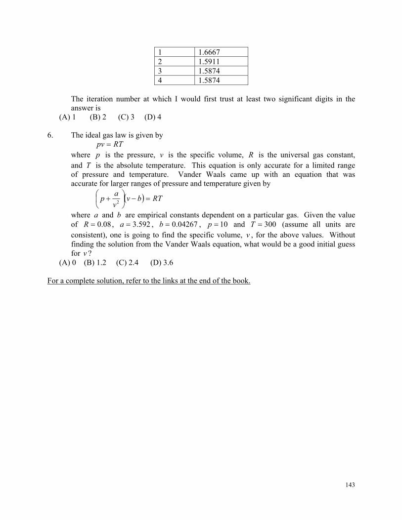
143

1 1.6667 2 1.5911 3 1.5874 4 1.5874

The iteration number at which I would first trust at least two significant digits in the answer is

(A) 1 (B) 2 (C) 3 (D) 4 6. The ideal gas law is given by RTpv where p is the pressure, v is the specific volume, R is the universal gas constant, and T is the absolute temperature. This equation is only accurate for a limited range of pressure and temperature. Vander Waals came up with an equation that was accurate for larger ranges of pressure and temperature given by

RTbvv

ap

2

where a and b are empirical constants dependent on a particular gas. Given the value of 08.0R , 592.3a , 04267.0b , 10p and 300T (assume all units are consistent), one is going to find the specific volume, v , for the above values. Without finding the solution from the Vander Waals equation, what would be a good initial guess for v ?

(A) 0 (B) 1.2 (C) 2.4 (D) 3.6 For a complete solution, refer to the links at the end of the book.

144

3.5 Chapter 03.05 Secant Method of Solving a Nonlinear Equation

PRE-REQUISITES

1. Know the definition of a derivative of a function (Primer for Differential Calculus). 2. Be able to find derivatives of function (Primer for Differential Calculus). 3. Know what a secant line is and how to find the equation of the secant line (Primer for

Differential Calculus).

OBJECTIVES 1. derive the secant method to solve for the roots of a nonlinear equation, 2. use the secant method to numerically solve a nonlinear equation.

After reading this chapter, you should be able to:

1. derive the secant method to solve for the roots of a nonlinear equation, 2. use the secant method to numerically solve a nonlinear equation.

What is the secant method and why would I want to use it instead of the Newton-Raphson method? The Newton-Raphson method of solving a nonlinear equation 0)( xf is given by the iterative formula

)(

)(1

i

iii xf

xf = xx

(1)

One of the drawbacks (dez avantajları) of the Newton-Raphson method is that you have to evaluate the derivative of the function. With availability of symbolic manipulators such as Maple, MathCAD, MATHEMATICA and MATLAB, this process has become more convenient. However, it still can be a laborious process, and even intractable if the function is derived as part of a numerical scheme. To overcome these drawbacks, the derivative of the function, )(xf is approximated as (Newton-Raphson yönteminin dez avantajlarından biri fonksiyonun türevinin olması gerektiğidir. Sembolik programlama dili kullanan Maple, MathCAD, MATHEMATICA ve MATLAB gibi programlar ile kök kolayca bulunabilir. Ancak, Newton-Raphson yönteminin uygulaması zahmetli ve fonksiyonun türevinin alınması gerektiğinden dolayı zordur. Bu dezavantajı )

1

1 )()()(

ii

iii xx

xfxfxf (2)

Substituting Equation (2) in Equation (1) gives

)()(

))((

1

11

ii

iiiii xfxf

xxxfxx (3)

The above equation is called the secant method. This method now requires two initial guesses, but unlike the bisection method, the two initial guesses do not need to bracket the root of the equation. The secant method is an open method and may or may not converge. However, when

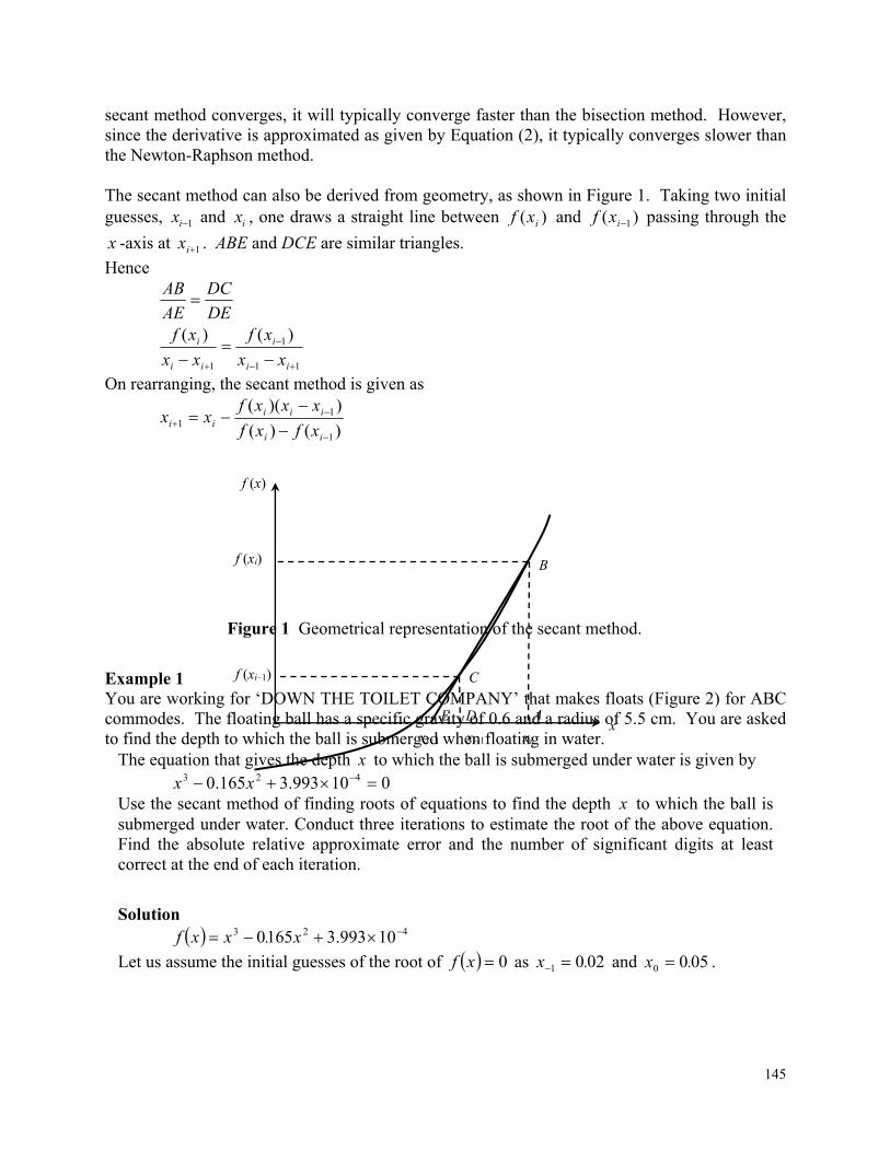
145

secant method converges, it will typically converge faster than the bisection method. However, since the derivative is approximated as given by Equation (2), it typically converges slower than the Newton-Raphson method. The secant method can also be derived from geometry, as shown in Figure 1. Taking two initial guesses, 1ix and ix , one draws a straight line between )( ixf and )( 1ixf passing through the

x -axis at 1ix . ABE and DCE are similar triangles.

Hence

DE

DC

AE

AB

11

1

1

)()(

ii

i

ii

i

xx

xf

xx

xf

On rearranging, the secant method is given as

)()(

))((

1

11

ii

iiiii xfxf

xxxfxx

Figure 1 Geometrical representation of the secant method.

Example 1 You are working for ‘DOWN THE TOILET COMPANY’ that makes floats (Figure 2) for ABC commodes. The floating ball has a specific gravity of 0.6 and a radius of 5.5 cm. You are asked to find the depth to which the ball is submerged when floating in water.

The equation that gives the depth x to which the ball is submerged under water is given by 010993.3165.0 423 xx

Use the secant method of finding roots of equations to find the depth x to which the ball is submerged under water. Conduct three iterations to estimate the root of the above equation. Find the absolute relative approximate error and the number of significant digits at least correct at the end of each iteration.

Solution 423 10993.31650 x.xxf

Let us assume the initial guesses of the root of 0xf as 0201 .x and 0500 .x .

f (x)

f (xi)

f (xi–1)

xi+1 xi–1 xi x

B

C

A D E

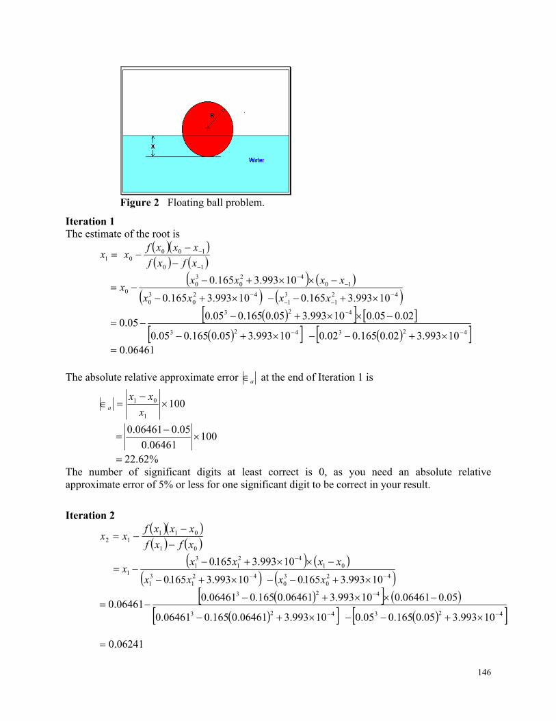
146

Figure 2 Floating ball problem.

Iteration 1 The estimate of the root is

1x 10

1000

xfxf

xxxfx

421

31

420

30

1042

030

010993.3165.010993.3165.0

10993.3165.0

xxxx

xxxxx

423423

423

10993.302.0165.002.010993.305.0165.005.0

02.005.010993.305.0165.005.005.0

06461.0 The absolute relative approximate error a at the end of Iteration 1 is

1001

01

x

xxa

10006461.0

05.006461.0

%62.22 The number of significant digits at least correct is 0, as you need an absolute relative approximate error of 5% or less for one significant digit to be correct in your result.

Iteration 2 01

01112 xfxf

xxxfxx

420

30

421

31

0142

131

110993.3165010993.31650

10993.31650

x.xx.x

xxx.xx

423423

423

10993.305.0165.005.010993.306461.0165.006461.0

05.006461.010993.306461.0165.006461.006461.0

06241.0

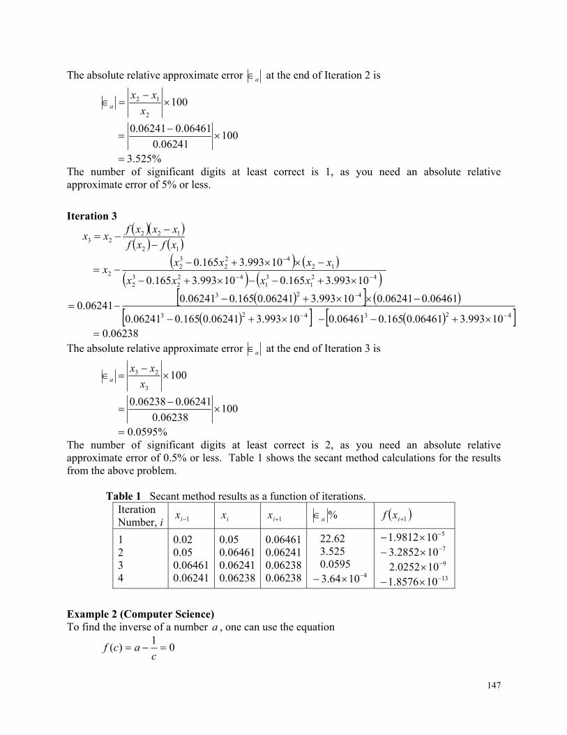
147

The absolute relative approximate error a at the end of Iteration 2 is

1002

12

x

xxa

10006241.0

06461.006241.0

%525.3 The number of significant digits at least correct is 1, as you need an absolute relative approximate error of 5% or less.

Iteration 3

12

12223 xfxf

xxxfxx

421

31

422

32

1242

232

210993.3165.010993.3165.0

10993.3165.0

xxxx

xxxxx

423423

423

10993.306461.0165.006461.010993.306241.0165.006241.0

06461.006241.010993.306241.0165.006241.006241.0

06238.0 The absolute relative approximate error a at the end of Iteration 3 is

1003

23

x

xxa

10006238.0

06241.006238.0

%0595.0 The number of significant digits at least correct is 2, as you need an absolute relative approximate error of 0.5% or less. Table 1 shows the secant method calculations for the results from the above problem. Table 1 Secant method results as a function of iterations.

Iteration Number, i 1ix ix 1ix %a

1ixf

1 2 3 4

0.02 0.05 0.06461 0.06241

0.05 0.06461 0.06241 0.06238

0.06461 0.06241 0.06238 0.06238

22.62 3.525 0.0595

41064.3

5109812.1 7102852.3

9100252.2 13108576.1

Example 2 (Computer Science) To find the inverse of a number a , one can use the equation

01

)( c

acf

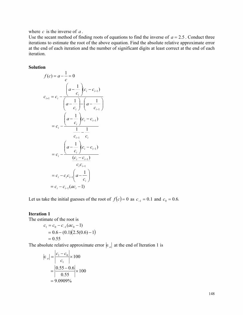
148

where c is the inverse of a . Use the secant method of finding roots of equations to find the inverse of 5.2a . Conduct three iterations to estimate the root of the above equation. Find the absolute relative approximate error at the end of each iteration and the number of significant digits at least correct at the end of each iteration.

Solution

01

)( c

acf

1

1

111

)(1

ii

iii

ii

ca

ca

ccc

a

cc

ii

iii

i

cc

ccc

a

c11

)(1

1

1

1

1

1

)(

)(1

ii

ii

iii

i

cc

cc

ccc

a

c

iiii c

accc1

1

)1(1 iii accc

Let us take the initial guesses of the root of 0cf as 1.01 c and .c 6.00

Iteration 1 The estimate of the root is )1( 0101 acccc

1)6.0(5.2)1.0(6.0 55.0 The absolute relative approximate error a at the end of Iteration 1 is

1001

01

c

cca

10055.0

6.055.0

%0909.9

149

The number of significant digits at least correct is 0, as you need an absolute relative approximate error of less than %5 for one significant digit to be correct in your result.

Iteration 2 The estimate of the root is

)1( 1012 acccc 1)55.0(5.2)6.0(55.0 325.0 The absolute relative approximate error a at the end of Iteration 2 is

1002

12

c

cca

100325.0

55.0325.0

%231.69 The number of significant digits at least correct is 0.

Iteration 3 The estimate of the root is )1( 2123 acccc

1)325.0(5.2)55.0(325.0 42813.0 The absolute relative approximate error a at the end of Iteration 3 is

1003

23

c

cca

10042813.0

325.042813.0

%088.24 The number of significant digits at least correct is 0.

Example 3 (Civil Engineering) You are making a bookshelf to carry books that range from 8½" (21.59cm) to 11" (27.94cm) in height and would take up 29" (73.66cm) of space along the length. The material is wood having a Young’s Modulus of Msi667.3 , thickness of 3/8" (0.9525cm) and width of 12" (30.48cm). You want to find the maximum vertical deflection of the bookshelf. The vertical deflection of the shelf is given by

xxxxxv 018507.010 66722.010 13533.010 42493.0)( 465834

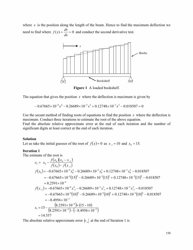
150

where x is the position along the length of the beam. Hence to find the maximum deflection we

need to find where 0)( dx

dvxf and conduct the second derivative test.

x

Books

Bookshelf

Figure 1 A loaded bookshelf. The equation that gives the position x where the deflection is maximum is given by

0018507.010 12748.010 26689.010 67665.0 233548 x xx Use the secant method of finding roots of equations to find the position x where the deflection is maximum. Conduct three iterations to estimate the root of the above equation. Find the absolute relative approximate error at the end of each iteration and the number of significant digits at least correct at the end of each iteration.

Solution Let us take the initial guesses of the root of 0xf as 101 x and .x 150

Iteration 1 The estimate of the root is

1x 10

1000

xfxf

xxxfx

018507.010 12748.010 26689.010 67665.0 20

330

540

80 x xx xf

018507.01510 12748.01510 26689.01510 67665.0 233548

4102591.8 018507.010 12748.010 26689.010 67665.0 2

133

154

18

1

x xx xf

018507.01010 12748.01010 26689.01010 67665.0 233548

3104956.8

34

4

1 104956.8102591.8

1015102591.815

x

557.14 The absolute relative approximate error a at the end of Iteration 1 is

151

1001

01

x

xxa

100557.14

15557.14

%0433.3 The number of significant digits at least correct is 1, because the absolute relative approximate error is less than %5 .

Iteration 2 The estimate of the root is

01

01112 xfxf

xxxfxx

018507.010 12748.010 26689.010 67665.0 21

331

541

81 x xx xf

018507.0557.1410 12748.0

557.1410 26689.0557.1410 67665.023

3548

5109870.2 45

5

2 102591.8109870.2

15557.14109870.215

x

572.14 The absolute relative approximate error a at the end of Iteration 2 is

1002

12

x

xxa

100572.14

557.14572.14

%10611.0 The number of significant digits at least correct is 2, because the absolute relative approximate error is less than %5.0 .

Iteration 3 The estimate of the root is

12

12223 xfxf

xxxfxx

018507.010 12748.010 26689.010 67665.0 22

332

542

82 x xx xf

018507.0572.1410 12748.0

572.1410 26689.0572.1410 67665.023

3548

9100676.6 59

9

3 109870.2100676.6

557.14572.14100676.6572.14

x

572.14

152

The absolute relative approximate error a at the end of Iteration 3 is

1003

23

x

xxa

100572.14

572.14572.14

%10 1559.2 5 The number of significant digits at least correct is 6, because the absolute relative approximate error is less than %00005.0 . Exercise . The average energy of vibration E of a molecule with frequency f depends on the temperature T according to the equation E = hf/(ehf/kT –1) + hf Here, h = 6.626×10–27 erg/sec. is Planck's constant and k=1.38×10–16 erg/°K is Boltzmann's constant. Find the frequency f of a molecule for which E = 3.97×10–14 erg and T = 31O°K.

NONLINEAR EQUATIONS Topic Secant Method for Solving Nonlinear Equations. Summary These are textbook notes of secant method of finding roots of nonlinear

equations. Derivations and examples are included. Major General Engineering Authors Autar Kaw Date Aralık 8, 2016 Web Site http://numericalmethods.eng.usf.edu

3.5.1 Multiple-Choice Test Secant Method Chapter 03.05 1. The secant method of finding roots of nonlinear equations falls under the category of

_____________ methods. (A) bracketing (B) graphical (C) open (D) random

2. The secant method formula for finding the square root of a real number R from the

equation 02 Rx is

(A) 1

1

ii

ii

xx

Rxx (B)

1

1

ii

ii

xx

xx (C)

ii x

Rx

2

1 (D)

1

122

ii

iii

xx

Rxxx

3. The next iterative value of the root of 042 x using secant method, if the initial

guesses are 3 and 4, is (A) 2.2857 (B) 2.5000 (C) 5.5000 (D) 5.7143

153

4. The root of the equation 0xf is found by using the secant method. Given one of the

initial estimates is 30 x , 53 f , and the angle the secant line makes with the x-axis is

57 , the next estimate of the root, 1x , is (A) –3.2470 (B) –0.24704 (C) 3.247 (D) 6.2470

5. For finding the root of 0 sin x by the secant method, the following choice of initial

guesses would not be appropriate.

(A) 4

and

2

(B)

4

and

4

3 (C)

2

and

2

(D)

3

and

2

6. When drugs are given orally to a patient, the drug concentration c in the blood stream at

time t is given by a formula atKtec where K is dependent on parameters such as the dose administered while a is dependent on the absorption and elimination rates of the drug. If 2K and 25.0a , and t is in seconds and c is in mlmg , the time at which the maximum concentration is reached is given by the solution of the equation

(A) 02 25.0 tte (B) 022 25.025.0 tt tee (C) 05.02 25.025.0 tt tee (D) 22 25.0 tte For a complete solution, refer to the links at the end of the book.

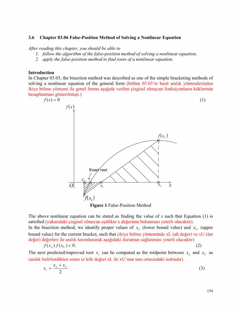
154

3.6 Chapter 03.06 False-Position Method of Solving a Nonlinear Equation After reading this chapter, you should be able to

1. follow the algorithm of the false-position method of solving a nonlinear equation, 2. apply the false-position method to find roots of a nonlinear equation.

Introduction In Chapter 03.03, the bisection method was described as one of the simple bracketing methods of solving a nonlinear equation of the general form (bölüm 03.03’te basit aralık yöntemlerinden ikiye bölme yöntemi ile genel formu aşağıda verilen çizgisel olmayan fonksiyonların köklerinin hesaplanması gösterilmişti.)

0)( xf (1)

Uxf

Uxrx

Lxf

Lx

O

xf

x

Figure 1 False-Position Method

The above nonlinear equation can be stated as finding the value of x such that Equation (1) is satisfied (yukarıdaki çizgisel olmayan eşitlikte x değerinin bulunması yeterli olacaktır). In the bisection method, we identify proper values of Lx (lower bound value) and Ux (upper

bound value) for the current bracket, such that (ikiye bölme yönteminde xL (alt değer) ve xU (üst değer) değerleri ile aralık tanımlanarak aşağıdaki durumun sağlanması yeterli olacaktır) 0)()( UL xfxf . (2)

The next predicted/improved root rx can be computed as the midpoint between Lx and Ux as

(aralık belirlendikten sonra xr kök değeri xL ile xU’nun tam ortasındaki noktadır)

2UL

r

xxx

(3)

155

The new upper and lower bounds are then established, and the procedure is repeated until the convergence is achieved (such that the new lower and upper bounds are sufficiently close to each other). (bu aşamadan sonra alt ve üst sınır değerleri yeniden tanımlanarak kök değerine yaklaşılır). However, in the example shown in Figure 1, the bisection method may not be efficient because it

does not take into consideration that )( Lxf is much closer to the zero of the function )(xf as

compared to )( Uxf . In other words, the next predicted root rx would be closer to Lx (in the

example as shown in Figure 1), than the mid-point between Lx and Ux . The false-position

method takes advantage of this observation mathematically by drawing a secant from the

function value at Lx to the function value at Ux , and estimates the root as where it crosses the x-

axis. (Şekil 1’den görüleceği gibi ikiye bölme yönteminde f(xL) fonksiyonunun değeri sıfıra çok yakınsa f(x) fonksiyonunun değeri f(xU)’ya doğru yaklaşmasından dolayı bu yöntem doğru kökü bulmada yeterli olmayabilir. Başka bir deyişle xL ile xU arasında olması gereken xr kök değeri xL’ye doğru yaklaşacaktır. False-position yöntemi bu aşamada xL’deki fonksiyon değerinden xU’daki fonksiyon değerine yatay ekseni kesen bir kiriş çizerek daha avantajlı olmaktadır.)

False-Position Method Based on two similar triangles, shown in Figure 1, one gets

Ur

U

Lr

L

xx

xf

xx

xf

)(0)(0 (4)

From Equation (4), one obtains LUrULr xfxxxfxx

ULrULLU xfxfxxfxxfx

The above equation can be solved to obtain the next predicted root mx as

UL

ULLUr xfxf

xfxxfxx

(5)

The above equation, through simple algebraic manipulations, can also be expressed as

UL

UL

UUr

xx

xfxf

xfxx (6)

or

LU

LU

LLr

xx

xfxf

xfxx (7)

Observe the resemblance of Equations (6) and (7) to the secant method.

False-Position Algorithm The steps to apply the false-position method to find the root of the equation 0xf are as follows.

156

1. Choose Lx and Ux as two guesses for the root such that 0UL xfxf , or in other words,

xf changes sign between Lx and Ux .

2. Estimate the root, rx of the equation 0xf as UL

ULLUr xfxf

xfxxfxx

3. Now check the following If 0rL xfxf , then the root lies between Lx and rx ; then LL xx and rU xx .

If 0rL xfxf , then the root lies between rx and Ux ; then rL xx and UU xx .

If 0rL xfxf , then the root is rx . Stop the algorithm. 4. Find the new estimate of the root

UL

ULLUr xfxf

xfxxfxx

Find the absolute relative approximate error as

100

newr

oldr

newr

a x

xx

where newrx = estimated root from present iteration oldrx = estimated root from previous iteration

5. Compare the absolute relative approximate error a with the pre-specified relative error

tolerance s . If sa , then go to step 3, else stop the algorithm. Note one should also check

whether the number of iterations is more than the maximum number of iterations allowed. If so, one needs to terminate the algorithm and notify the user about it. Note that the false-position and bisection algorithms are quite similar. The only difference is the formula used to calculate the new estimate of the root rx as shown in steps #2 and #4!

Example 1 You are working for “DOWN THE TOILET COMPANY” that makes floats for ABC commodes. The floating ball has a specific gravity of 0.6 and has a radius of 5.5cm. You are asked to find the depth to which the ball is submerged when floating in water. The equation that gives the depth x to which the ball is submerged under water is given by

010993.3165.0 423 xx Use the false-position method of finding roots of equations to find the depth x to which the ball is submerged under water. Conduct three iterations to estimate the root of the above equation. Find the absolute relative approximate error at the end of each iteration, and the number of significant digits at least correct at the end of third iteration.

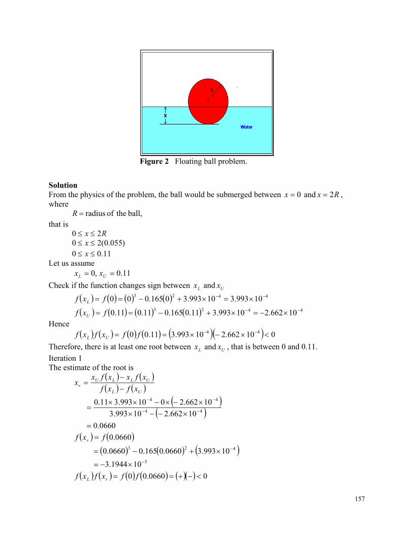
157

Figure 2 Floating ball problem.

Solution From the physics of the problem, the ball would be submerged between 0x and Rx 2 , where ball, theof radiusR that is Rx 20 )055.0(20 x 11.00 x Let us assume

11.0,0 UL xx

Check if the function changes sign between Lx and Ux

4423

4423

10662.210993.311.0165.011.011.0

10993.310993.30165.000

fxf

fxf

U

L

Hence 010662.210993.311.00 44 ffxfxf UL

Therefore, there is at least one root between Lx and Ux , that is between 0 and 0.11.

Iteration 1 The estimate of the root is

0660.0

10662.210993.3

10662.2010993.311.044

44

UL

ULLUr xfxf

xfxxfxx

5

423

101944.3

10993.30660.0165.00660.0

0660.0

fxf r

00660.00 ffxfxf rL

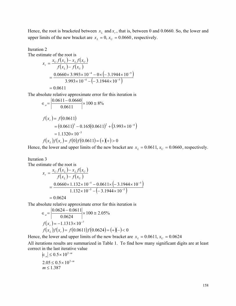
158

Hence, the root is bracketed between Lx and rx , that is, between 0 and 0.0660. So, the lower and

upper limits of the new bracket are 0660.0,0 UL xx , respectively.

Iteration 2 The estimate of the root is

0611.0

101944.310993.3

101944.3010993.30660.054

54

UL

ULLUr xfxf

xfxxfxx

The absolute relative approximate error for this iteration is

%81000611.0

0660.00611.0

a

5

423

101320.1

10993.30611.0165.00611.0

0611.0

fxf r

00611.00 ffxfxf rL

Hence, the lower and upper limits of the new bracket are 0660.0,0611.0 UL xx , respectively.

Iteration 3 The estimate of the root is

0624.0

101944.310132.1

101944.30611.010132.10660.055

55

UL

ULLUr xfxf

xfxxfxx

The absolute relative approximate error for this iteration is

%05.21000624.0

0611.00624.0

a

7101313.1 rxf

00624.00611.0 ffxfxf rL

Hence, the lower and upper limits of the new bracket are 0624.0,0611.0 UL xx

All iterations results are summarized in Table 1. To find how many significant digits are at least correct in the last iterative value

m

ma

2

2

105.005.2

105.0

387.1m

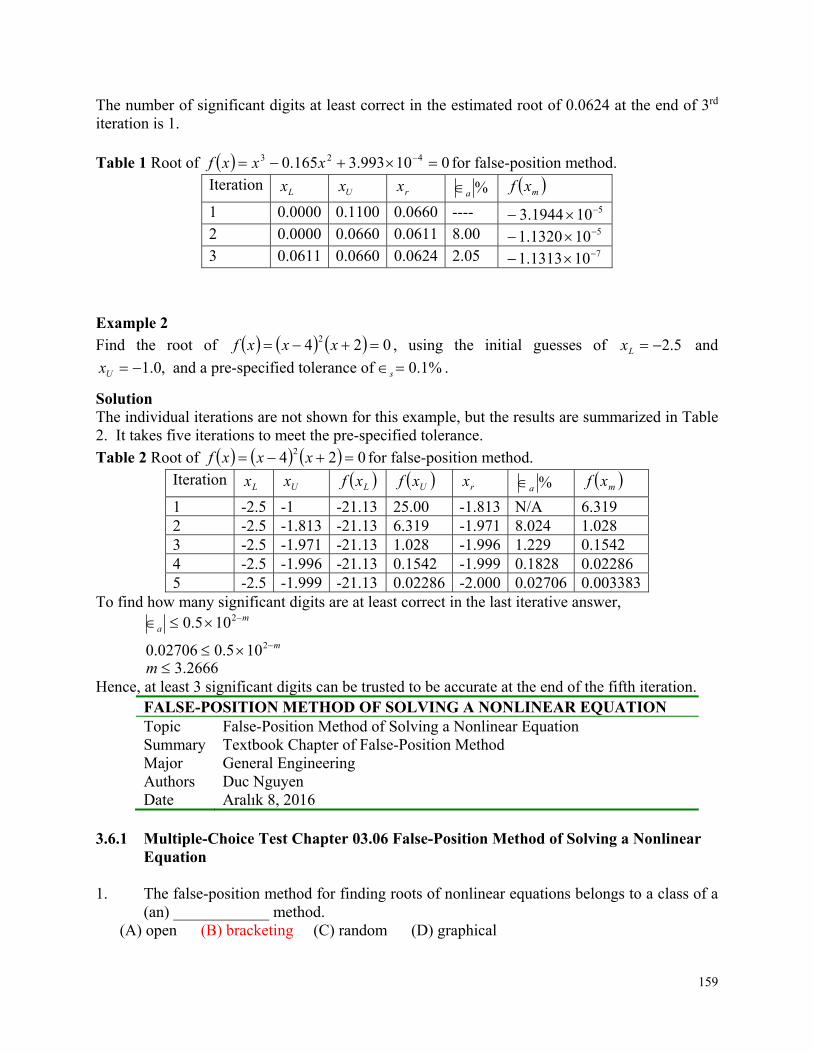
159

The number of significant digits at least correct in the estimated root of 0.0624 at the end of 3rd

iteration is 1. Table 1 Root of 010993.3165.0 423 xxxf for false-position method.

Iteration Lx Ux rx %a

mxf 1 0.0000 0.1100 0.0660 ---- 5101944.3 2 0.0000 0.0660 0.0611 8.00 5101320.1 3 0.0611 0.0660 0.0624 2.05 7101313.1

Example 2 Find the root of 024 2 xxxf , using the initial guesses of 5.2Lx and

,0.1Ux and a pre-specified tolerance of %1.0s .

Solution The individual iterations are not shown for this example, but the results are summarized in Table 2. It takes five iterations to meet the pre-specified tolerance.

Table 2 Root of 024 2 xxxf for false-position method. Iteration

Lx Ux Lxf Uxf rx %a mxf

1 -2.5 -1 -21.13 25.00 -1.813 N/A 6.319 2 -2.5 -1.813 -21.13 6.319 -1.971 8.024 1.028 3 -2.5 -1.971 -21.13 1.028 -1.996 1.229 0.1542 4 -2.5 -1.996 -21.13 0.1542 -1.999 0.1828 0.02286 5 -2.5 -1.999 -21.13 0.02286 -2.000 0.02706 0.003383

To find how many significant digits are at least correct in the last iterative answer,

m

ma

2

2

105.002706.0

105.0

2666.3m Hence, at least 3 significant digits can be trusted to be accurate at the end of the fifth iteration.

FALSE-POSITION METHOD OF SOLVING A NONLINEAR EQUATION Topic False-Position Method of Solving a Nonlinear Equation Summary Textbook Chapter of False-Position Method Major General Engineering Authors Duc Nguyen Date Aralık 8, 2016

3.6.1 Multiple-Choice Test Chapter 03.06 False-Position Method of Solving a Nonlinear

Equation 1. The false-position method for finding roots of nonlinear equations belongs to a class of a

(an) ____________ method. (A) open (B) bracketing (C) random (D) graphical

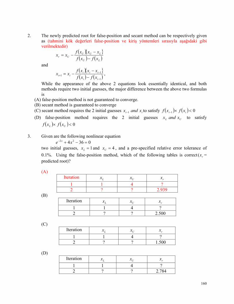
160

2. The newly predicted root for false-position and secant method can be respectively given

as (tahmini kök değerleri false-position ve kiriş yöntemleri sırasıyla aşağıdaki gibi verilmektedir)

LU

LUUUr xfxf

xxxfxx

and 1

11

ii

iiiii xfxf

xxxfxx ,

While the appearance of the above 2 equations look essentially identical, and both methods require two initial guesses, the major difference between the above two formulas is

(A) false-position method is not guaranteed to converge. (B) secant method is guaranteed to converge (C) secant method requires the 2 initial guesses ii xandx 1 to satisfy 01 ii xfxf

(D) false-position method requires the 2 initial guesses UL xandx to satisfy

0 UL xfxf

3. Given are the following nonlinear equation

0364 22 xe x two initial guesses, 1Lx and 4Ux , and a pre-specified relative error tolerance of

0.1%. Using the false-position method, which of the following tables is correct rx( = predicted root)? (A)

Iteration Lx Ux rx

1 1 4 ? 2 ? ? 2.939

(B) Iteration

Lx Ux rx

1 1 4 ? 2 ? ? 2.500

(C)

Iteration Lx Ux rx

1 1 4 ? 2 ? ? 1.500

(D)

Iteration Lx Ux rx

1 1 4 ? 2 ? ? 2.784

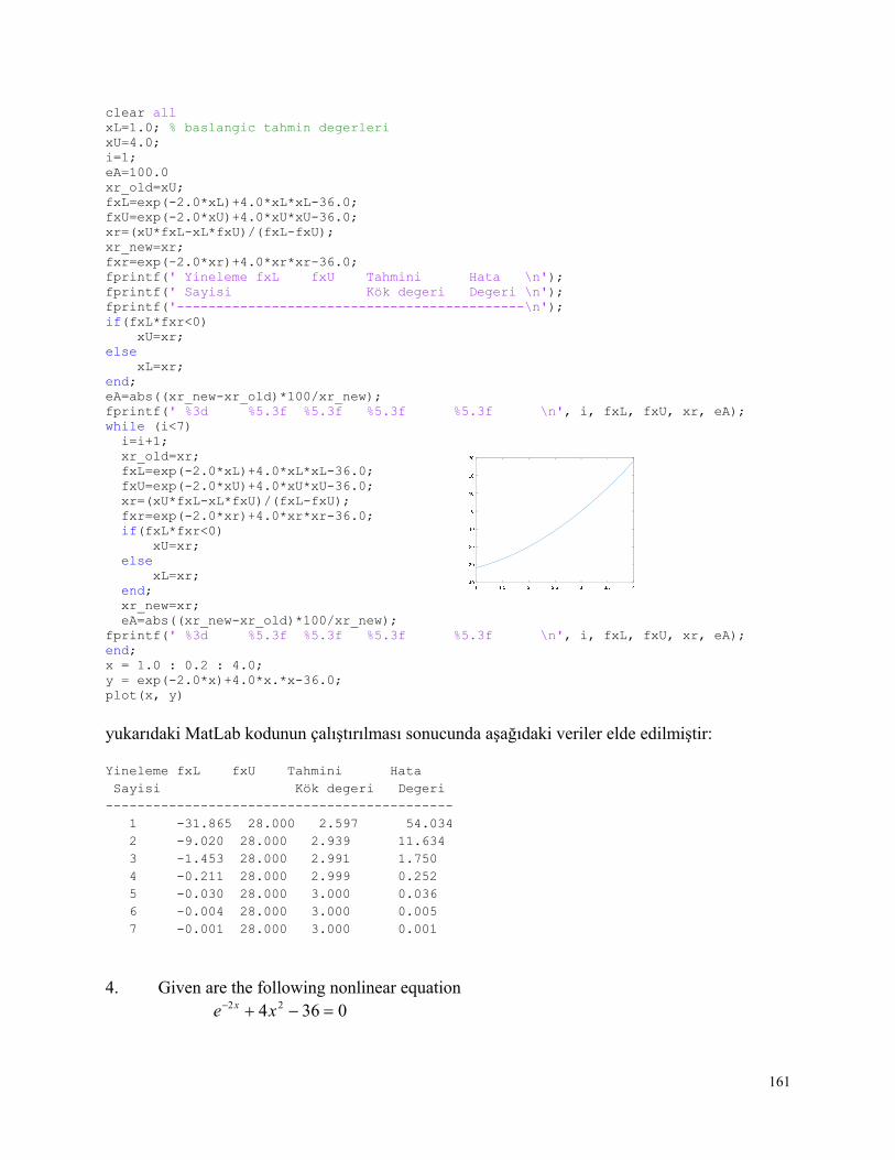
161

clear all xL=1.0; % baslangic tahmin degerleri xU=4.0; i=1; eA=100.0 xr_old=xU; fxL=exp(-2.0*xL)+4.0*xL*xL-36.0; fxU=exp(-2.0*xU)+4.0*xU*xU-36.0; xr=(xU*fxL-xL*fxU)/(fxL-fxU); xr_new=xr; fxr=exp(-2.0*xr)+4.0*xr*xr-36.0; fprintf(' Yineleme fxL fxU Tahmini Hata \n'); fprintf(' Sayisi Kök degeri Degeri \n'); fprintf('--------------------------------------------\n'); if(fxL*fxr<0) xU=xr; else xL=xr; end; eA=abs((xr_new-xr_old)*100/xr_new); fprintf(' %3d %5.3f %5.3f %5.3f %5.3f \n', i, fxL, fxU, xr, eA); while (i<7) i=i+1; xr_old=xr; fxL=exp(-2.0*xL)+4.0*xL*xL-36.0; fxU=exp(-2.0*xU)+4.0*xU*xU-36.0; xr=(xU*fxL-xL*fxU)/(fxL-fxU); fxr=exp(-2.0*xr)+4.0*xr*xr-36.0; if(fxL*fxr<0) xU=xr; else xL=xr; end; xr_new=xr; eA=abs((xr_new-xr_old)*100/xr_new); fprintf(' %3d %5.3f %5.3f %5.3f %5.3f \n', i, fxL, fxU, xr, eA); end; x = 1.0 : 0.2 : 4.0; y = exp(-2.0*x)+4.0*x.*x-36.0; plot(x, y) yukarıdaki MatLab kodunun çalıştırılması sonucunda aşağıdaki veriler elde edilmiştir: Yineleme fxL fxU Tahmini Hata Sayisi Kök degeri Degeri -------------------------------------------- 1 -31.865 28.000 2.597 54.034 2 -9.020 28.000 2.939 11.634 3 -1.453 28.000 2.991 1.750 4 -0.211 28.000 2.999 0.252 5 -0.030 28.000 3.000 0.036 6 -0.004 28.000 3.000 0.005 7 -0.001 28.000 3.000 0.001

4. Given are the following nonlinear equation

0364 22 xe x

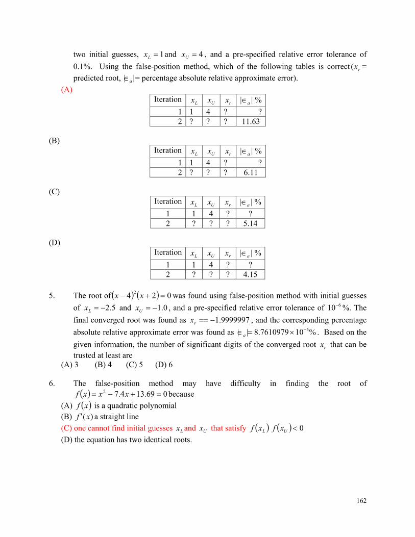
162

two initial guesses, 1Lx and 4Ux , and a pre-specified relative error tolerance of

0.1%. Using the false-position method, which of the following tables is correct rx( =

predicted root, || a = percentage absolute relative approximate error).

(A) Iteration

Lx Ux rx | a | %

1 1 4 ? ? 2 ? ? ? 11.63

(B)

Iteration Lx Ux rx | a | %

1 1 4 ? ? 2 ? ? ? 6.11

(C)

Iteration Lx Ux rx | a | %

1 1 4 ? ? 2 ? ? ? 5.14

(D)

Iteration Lx Ux rx | a | %

1 1 4 ? ? 2 ? ? ? 4.15

5. The root of 024 2 xx was found using false-position method with initial guesses

of 5.2Lx and 0.1Ux , and a pre-specified relative error tolerance of 610 %. The

final converged root was found as 9999997.1rx , and the corresponding percentage

absolute relative approximate error was found as %107610979.8|| 5a . Based on the

given information, the number of significant digits of the converged root rx that can be trusted at least are

(A) 3 (B) 4 (C) 5 (D) 6 6. The false-position method may have difficulty in finding the root of

069.134.72 xxxf because

(A) xf is a quadratic polynomial (B) )(xf a straight line

(C) one cannot find initial guesses Lx and Ux that satisfy 0UL xfxf

(D) the equation has two identical roots.

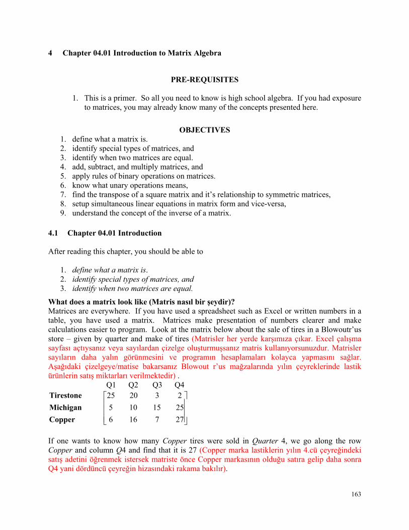
163

4 Chapter 04.01 Introduction to Matrix Algebra

PRE-REQUISITES

1. This is a primer. So all you need to know is high school algebra. If you had exposure to matrices, you may already know many of the concepts presented here.

OBJECTIVES 1. define what a matrix is. 2. identify special types of matrices, and 3. identify when two matrices are equal. 4. add, subtract, and multiply matrices, and 5. apply rules of binary operations on matrices. 6. know what unary operations means, 7. find the transpose of a square matrix and it’s relationship to symmetric matrices, 8. setup simultaneous linear equations in matrix form and vice-versa, 9. understand the concept of the inverse of a matrix.

4.1 Chapter 04.01 Introduction After reading this chapter, you should be able to

1. define what a matrix is. 2. identify special types of matrices, and 3. identify when two matrices are equal.

What does a matrix look like (Matris nasıl bir şeydir)? Matrices are everywhere. If you have used a spreadsheet such as Excel or written numbers in a table, you have used a matrix. Matrices make presentation of numbers clearer and make calculations easier to program. Look at the matrix below about the sale of tires in a Blowoutr’us store – given by quarter and make of tires (Matrisler her yerde karşımıza çıkar. Excel çalışma sayfası açtıysanız veya sayılardan çizelge oluşturmuşsanız matris kullanıyorsunuzdur. Matrisler sayıların daha yalın görünmesini ve programın hesaplamaları kolayca yapmasını sağlar. Aşağıdaki çizelgeye/matise bakarsanız Blowout r’us mağzalarında yılın çeyreklerinde lastik ürünlerin satış miktarları verilmektedir) . Q1 Q2 Q3 Q4

Copper

Michigan

Tirestone

6

5

25

16

10

20

7

15

3

27

25

2

If one wants to know how many Copper tires were sold in Quarter 4, we go along the row Copper and column Q4 and find that it is 27 (Copper marka lastiklerin yılın 4.cü çeyreğindeki satış adetini öğrenmek istersek matriste önce Copper markasının olduğu satıra gelip daha sonra Q4 yani dördüncü çeyreğin hizasındaki rakama bakılır).

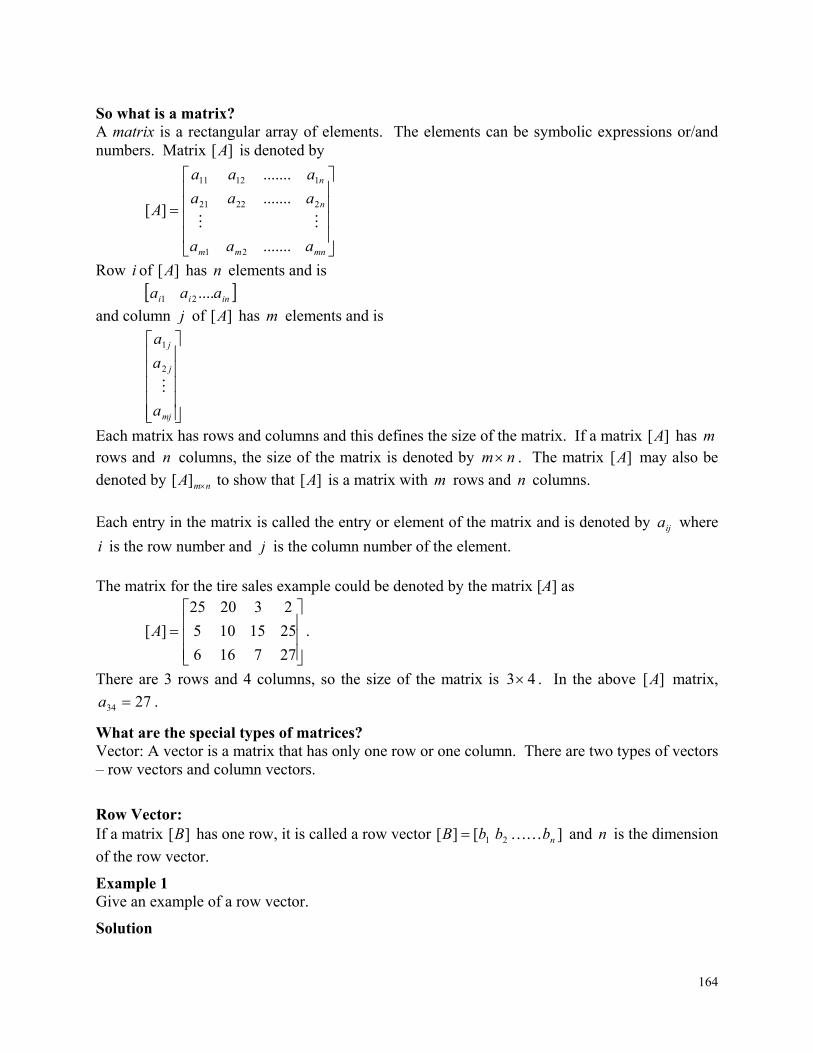
164

So what is a matrix? A matrix is a rectangular array of elements. The elements can be symbolic expressions or/and numbers. Matrix ][A is denoted by

mnmm

n

n

aaa

aaa

aaa

A

.......

.......

.......

][

21

22221

11211

Row i of ][A has n elements and is

inii aaa ....2 1

and column j of ][A has m elements and is

mj

j

j

a

a

a

2

1

Each matrix has rows and columns and this defines the size of the matrix. If a matrix ][A has m rows and n columns, the size of the matrix is denoted by nm . The matrix ][A may also be

denoted by nmA ][ to show that ][A is a matrix with m rows and n columns.

Each entry in the matrix is called the entry or element of the matrix and is denoted by ija where

i is the row number and j is the column number of the element. The matrix for the tire sales example could be denoted by the matrix [A] as

277166

2515105

232025

][A .

There are 3 rows and 4 columns, so the size of the matrix is 43 . In the above ][A matrix,

2734 a .

What are the special types of matrices? Vector: A vector is a matrix that has only one row or one column. There are two types of vectors – row vectors and column vectors.

Row Vector: If a matrix ][B has one row, it is called a row vector ][][ 21 nbbbB and n is the dimension

of the row vector.

Example 1 Give an example of a row vector.

Solution

165

]0232025[][ B is an example of a row vector of dimension 5.

Column vector: If a matrix ][C has one column, it is called a column vector

mc

c

C1

][

and m is the dimension of the vector.

Example 2 Give an example of a column vector.

Solution

6

5

25

][C

is an example of a column vector of dimension 3.

Submatrix: If some row(s) or/and column(s) of a matrix ][A are deleted (no rows or columns may be deleted), the remaining matrix is called a submatrix of ][A .

Example 3 Find some of the submatrices of the matrix

213

264][A

Solution

2

2,4,264,

13

64,

213

264

are some of the submatrices of ][A . Can you find other submatrices of ][A ?

Square matrix: If the number of rows m of a matrix is equal to the number of columns n of a matrix ][A , that

is, nm , then ][A is called a square matrix. The entries nnaaa ,...,, 2211 are called the diagonal

elements of a square matrix. Sometimes the diagonal of the matrix is also called the principal or main of the matrix.

Example 4 Give an example of a square matrix.

166

Solution

7156

15105

32025

][A

is a square matrix as it has the same number of rows and columns, that is, 3. The diagonal elements of ][A are 7,10,25 332211 aaa .

Upper triangular matrix: A nn matrix for which jiaij ,0 for all ji, is called an upper triangular matrix. That is,

all the elements below the diagonal entries are zero.

Example 5 Give an example of an upper triangular matrix.

Solution

1500500

6001.00

0710

][A

is an upper triangular matrix.

Lower triangular matrix: A nn matrix for which ijaij ,0 for all ji, is called a lower triangular matrix. That is, all

the elements above the diagonal entries are zero.

Example 6 Give an example of a lower triangular matrix.

Solution

15.26.0

013.0

001

][A

is a lower triangular matrix.

Diagonal matrix: A square matrix with all non-diagonal elements equal to zero is called a diagonal matrix, that is, only the diagonal entries of the square matrix can be non-zero, ( jiaij ,0 ).

Example 7 Give examples of a diagonal matrix.

Solution

167

500

01.20

003

][A

is a diagonal matrix. Any or all the diagonal entries of a diagonal matrix can be zero. For example

000

01.20

003

][A

is also a diagonal matrix.

Identity matrix: A diagonal matrix with all diagonal elements equal to 1 is called an identity matrix, ( jiaij ,0 for all ji, and 1iia for all i ).

Example 8 Give an example of an identity matrix.

Solution

1000

0100

0010

0001

][A

is an identity matrix.

Zero matrix: A matrix whose all entries are zero is called a zero matrix, ( 0ija for all i and j ).

Example 9 Give examples of a zero matrix.

Solution

000

000

000

][A

0 0 0

0 0 0 [B]

0

0

0

000

000

000

][C

000][ D are all examples of a zero matrix.

168

Tridiagonal matrices: A tridiagonal matrix is a square matrix in which all elements not on the following are zero - the major diagonal, the diagonal above the major diagonal, and the diagonal below the major diagonal.

Example 10 Give an example of a tridiagonal matrix.

Solution

6300

2500

0932

0042

][A

is a tridiagonal matrix.

Do non-square matrices have diagonal entries? Yes, for a nm matrix ][A , the diagonal entries are kkkk aaaa ,...,, 1,12211 where },min{ nmk .

Example 11 What are the diagonal entries of

8.76.5

2.39.2

76

52.3

][A

Solution The diagonal elements of ][A are .7 and 2.3 2211 aa

Diagonally Dominant Matrix: A nn square matrix ][A is a diagonally dominant matrix if

n

jij

ijii aa1

|| for ni ,.....,2,1 and

n

jij

ijii aa1

|| for at least one i ,

that is, for each row, the absolute value of the diagonal element is greater than or equal to the sum of the absolute values of the rest of the elements of that row, and that the inequality is strictly greater than for at least one row. Diagonally dominant matrices are important in ensuring convergence in iterative schemes of solving simultaneous linear equations.

Example 12 Give examples of diagonally dominant matrices and not diagonally dominant matrices.

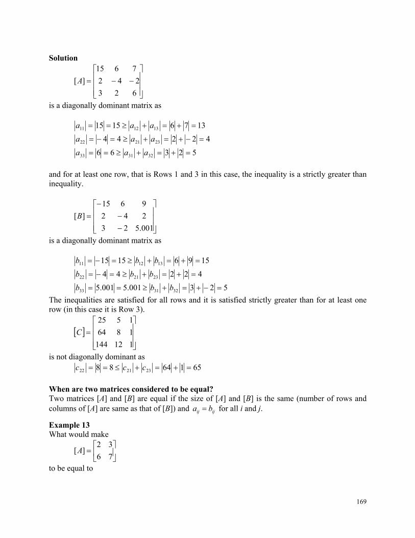
169

Solution

623

242

7615

][A

is a diagonally dominant matrix as

13761515 131211 aaa

42244 232122 aaa

52366 323133 aaa

and for at least one row, that is Rows 1 and 3 in this case, the inequality is a strictly greater than inequality.

001.523

242

9615

][B

is a diagonally dominant matrix as 15961515 131211 bbb

42244 232122 bbb

523001.5001.5 323133 bbb

The inequalities are satisfied for all rows and it is satisfied strictly greater than for at least one row (in this case it is Row 3).

112144

1864

1525

C

is not diagonally dominant as 6516488 232122 ccc

When are two matrices considered to be equal? Two matrices [A] and [B] are equal if the size of [A] and [B] is the same (number of rows and columns of [A] are same as that of [B]) and ijij ba for all i and j.

Example 13 What would make

76

32][A

to be equal to

170

22

11

6

3][

b

bB

Solution The two matrices ][A and ][B ould be equal if 211 b and 722 b .

Key Terms: Matrix Vector Submatrix Square matrix Equal matrices Zero matrix Identity matrix Diagonal matrix Upper triangular matrix Lower triangular matrix Tri-diagonal matrix Diagonally dominant matrix 4.2 Chapter 04.02 Vectors After reading this chapter, you should be able to:

1. define a vector, 2. add and subtract vectors, 3. find linear combinations of vectors and their relationship to a set of equations, 4. explain what it means to have a linearly independent set of vectors, and 5. find the rank of a set of vectors.

What is a vector? A vector is a collection of numbers in a definite order. If it is a collection of n numbers, it is

called a n -dimensional vector. So the vector A

given by

171

na

a

a

A

2

1

is a n -dimensional column vector with n components, naaa ,......,, 21 . The above is a column

vector. A row vector ][B is of the form ],....,,[ 21 nbbbB

where B

is a n -dimensional row

vector with n components nbbb ,....,, 21 .

Example 1 Give an example of a 3-dimensional column vector.

Solution Assume a point in space is given by its ),,( zyx coordinates. Then if the value of

5,2,3 zyx , the column vector corresponding to the location of the points is

5

2

3

z

y

x

.

When are two vectors equal? Two vectors A

and B

are equal if they are of the same dimension and if their corresponding

components are equal. Given

na

a

a

A

2

1

and

nb

b

b

B

2

1

then BA

if niba ii ,......,2,1, .

Example 2 What are the values of the unknown components in B

if

172

1

4

3

2

A

and

4

1

4

3

b

b

B

and BA

.

Solution 1 ,2 41 bb

How do you add two vectors? Two vectors can be added only if they are of the same dimension and the addition is given by

nn b

b

b

a

a

a

BA2

1

2

1

][][

nn ba

ba

ba

22

11

Example 3 Add the two vectors

1

4

3

2

A

and

7

3

2

5

B

Solution

173

7

3

2

5

1

4

3

2

BA

71

34

23

52

8

7

1

7

Example 4 A store sells three brands of tires: Tirestone, Michigan and Copper. In quarter 1, the sales are given by the column vector

6

5

25

1A

where the rows represent the three brands of tires sold – Tirestone, Michigan and Copper respectively. In quarter 2, the sales are given by

6

10

20

2A

What is the total sale of each brand of tire in the first half of the year?

Solution The total sales would be given by

21 AAC

6

10

20

6

5

25

66

105

2025

174

12

15

45

So the number of Tirestone tires sold is 45, Michigan is 15 and Copper is 12 in the first half of the year.

What is a null vector? A null vector (also called zero vector) is where all the components of the vector are zero.

Example 5 Give an example of a null vector or zero vector.

Solution The vector

0

0

0

0

is an example of a zero or null vector.

What is a unit vector? A unit vector U

is defined as

nu

u

u

U

2

1

where

1223

22

21 nuuuu

Example 6 Give examples of 3-dimensional unit column vectors.

Solution Examples include

,

0

1

0

,

02

12

1

,

0

0

1

,

3

13

13

1

etc.

175

How do you multiply a vector by a scalar? If k is a scalar and A

is a n -dimensional vector, then

na

a

a

kAk

2

1

nka

ka

ka

2

1

Example 7 What is A

2 if

5

20

25

A

Solution

5

20

25

22A

52

202

252

10

40

50

Example 8 A store sells three brands of tires: Tirestone, Michigan and Copper. In quarter 1, the sales are given by the column vector

6

25

25

A

If the goal is to increase the sales of all tires by at least 25% in the next quarter, how many of each brand should be sold?

176

Solution Since the goal is to increase the sales by 25%, one would multiply the A

vector by 1.25,

6

25

25

25.1B

5.7

25.31

25.31

Since the number of tires must be an integer, we can say that the goal of sales is

8

32

32

B

What do you mean by a linear combination of vectors? Given

mAAA

,......,, 21

as m vectors of same dimension n, and if mkkk ,...,, 21 are scalars, then

mm AkAkAk

.......2211

is a linear combination of the m vectors.

Example 9 Find the linear combinations

a) BA

and

b) CBA

3 where

2

1

10

,

2

1

1

,

6

3

2

CBA

Solution

a)

2

1

1

6

3

2

BA

26

13

12

177

4

2

1

b)

2

1

10

3

2

1

1

6

3

2

3CBA

626

313

3012

2

1

27

What do you mean by vectors being linearly independent?

A set of vectors mAAA

,,, 21 are considered to be linearly independent if

0.......2211

mm AkAkAk

has only one solution of 0......21 mkkk

Example 10 Are the three vectors

1

1

1

,

12

8

5

,

144

64

25

321 AAA

linearly independent?

Solution Writing the linear combination of the three vectors

0

0

0

1

1

1

12

8

5

144

64

25

321 kkk

gives

0

0

0

12144

864

525

321

321

321

kkk

kkk

kkk

178

The above equations have only one solution, 0321 kkk . However, how do we show that

this is the only solution? This is shown below. The above equations are 0525 321 kkk (1)

0864 321 kkk (2)

012144 321 kkk (3)

Subtracting Eqn (1) from Eqn (2) gives 0339 21 kk

12 13kk (4) Multiplying Eqn (1) by 8 and subtracting it from Eqn (2) that is first multiplied by 5 gives 03120 31 kk

13 40kk (5)

Remember we found Eqn (4) and Eqn (5) just from Eqns (1) and (2). Substitution of Eqns (4) and (5) in Eqn (3) for 1k and 2k gives

040)13(12144 111 kkk

028 1 k

01 k

This means that 1k has to be zero, and coupled with (4) and (5), 2k and 3k are also zero. So the

only solution is 0321 kkk . The three vectors hence are linearly independent.

Example 11 Are the three vectors

24

14

6

,

7

5

2

,

5

2

1

321 AAA

linearly independent?

Solution By inspection,

213 22 AAA

or

022 321

AAA

So the linear combination

0332211

AkAkAk

has a non-zero solution 1,2,2 321 kkk

Hence, the set of vectors is linearly dependent. What if I cannot prove by inspection, what do I do? Put the linear combination of three vectors equal to the zero vector,

179

0

0

0

24

14

6

7

5

2

5

2

1

321 kkk

to give 062 321 kkk (1)

01452 321 kkk (2)

02475 321 kkk (3)

Multiplying Eqn (1) by 2 and subtracting from Eqn (2) gives 02 32 kk

32 2kk (4)

Multiplying Eqn (1) by 2.5 and subtracting from Eqn (2) gives 05.0 31 kk

31 2kk (5)

Remember we found Eqn (4) and Eqn (5) just from Eqns (1) and (2). Substitute Eqn (4) and (5) in Eqn (3) for 1k and 2k gives

0242725 333 kkk

0241410 333 kkk

00 This means any values satisfying Eqns (4) and (5) will satisfy Eqns (1), (2) and (3) simultaneously. For example, chose 63 k , then

122 k from Eqn (4), and

121 k from Eqn (5).

Hence we have a nontrivial solution of 61212321 kkk . This implies the three

given vectors are linearly dependent. Can you find another nontrivial solution? What about the following three vectors?

25

14

6

,

7

5

2

,

5

2

1

Are they linearly dependent or linearly independent? Note that the only difference between this set of vectors and the previous one is the third entry in the third vector. Hence, equations (4) and (5) are still valid. What conclusion do you draw when you plug in equations (4) and (5) in the third equation: 02575 321 kkk ? What has

changed?

Example 12 Are the three vectors

180

2

1

1

,

13

8

5

,

89

64

25

321 AAA

linearly independent?

Solution Writing the linear combination of the three vectors and equating to zero vector

0

0

0

2

1

1

13

8

5

89

64

25

321 kkk

gives

0

0

0

21389

864

525

321

321

321

kkk

kkk

kkk

In addition to 0321 kkk , one can find other solutions for which 321 ,, kkk are not equal to

zero. For example, 40,13,1 321 kkk is also a solution as

0

0

0

2

1

1

40

13

8

5

13

89

64

25

1

Hence 321 ,, AAA

are linearly dependent.

What do you mean by the rank of a set of vectors? From a set of n -dimensional vectors, the maximum number of linearly independent vectors in the set is called the rank of the set of vectors. Note that the rank of the vectors can never be greater than the vectors dimension.

Example 13 What is the rank of

1

1

1

,

12

8

5

,

144

64

25

321 AAA

?

Solution Since we found in Example 2.10 that 321 ,, AAA

are linearly independent, the rank of the set of

vectors 321 ,, AAA

is 3. If we were given another vector 4A

, the rank of the set of the vectors

4321 ,,, AAAA

would still be 3 as the rank of a set of vectors is always less than or equal to the

dimension of the vectors and that at least 321 ,, AAA

are linearly independent.

181

Example 14 What is the rank of

2

1

1

,

13

8

5

,

89

64

25

321 AAA

?

Solution In Example 2.12, we found that 321 ,, AAA

are linearly dependent, the rank of 321 ,, AAA

is hence

not 3, and is less than 3. Is it 2? Let us choose two of the three vectors

13

8

5

,

89

64

25

21 AA

Linear combination of 1A

and 2A

equal to zero has only one solution – the trivial solution. Therefore, the rank is 2.

Example 15 What is the rank of

5

3

3

,

4

2

2

,

2

1

1

321 AAA

?

Solution From inspection,

12 2AA

, that implies

.002 321

AAA

Hence

.0332211

AkAkAk

has a nontrivial solution.

So 321 ,, AAA

are linearly dependent, and hence the rank of the three vectors is not 3. Since

12 2AA

,

21 and AA

are linearly dependent, but

.03311

AkAk

has trivial solution as the only solution. So 31 and AA

are linearly independent. The rank of the

above three vectors is 2. Prove that if a set of vectors contains the null vector, the set of vectors is linearly dependent.

182

Let mAAA

,,........., 21 be a set of n -dimensional vectors, then

02211

mm AkAkAk

is a linear combination of the m vectors. Then assuming if 1A

is the zero or null vector, any

value of 1k coupled with 032 mkkk will satisfy the above equation. Hence, the set of

vectors is linearly dependent as more than one solution exists.

Prove that if a set of m vectors is linearly independent, then a subset of the m vectors also

has to be linearly independent. Let this subset of vectors be

apaa AAA

,,, 21

where mp . Then if this subset of vectors is linearly dependent, the linear combination

02211

appaa AkAkAk

has a non-trivial solution. So

00.......0 )1(2211

ampaappaa AAAkAkAk

also has a non-trivial solution too, where ampa AA

,,1 are the rest of the )( pm vectors.

However, this is a contradiction. Therefore, a subset of linearly independent vectors cannot be linearly dependent.

Prove that if a set of vectors is linearly dependent, then at least one vector can be written as

a linear combination of others.

Let mAAA

,,, 21 be linearly dependent set of vectors, then there exists a set of scalars

mkk ,,1 not all of which are zero for the linear combination equation

02211

mm AkAkAk .

Let pk be one of the non-zero values of miki ,,1, , that is, 0pk , then

.11

11

22

mp

mp

p

pp

p

p

pp A

k

kA

k

kA

k

kA

k

kA

and that proves the theorem.

Prove that if the dimension of a set of vectors is less than the number of vectors in the set,

then the set of vectors is linearly dependent. Can you prove it?

How can vectors be used to write simultaneous linear equations? If a set of m simultaneous linear equations with n unknowns is written as 11111 cxaxa nn

183

22121 cxaxa nn

nnmnm cxaxa 11

where nxxx ,,, 21 are the unknowns, then in the vector notation they can be written as

CAxAxAx nn

2211

where

1

11

1

ma

a

A

where

1

11

1

ma

a

A

2

12

2

ma

a

A

mn

n

n

a

a

A 1

mc

c

C 1

1

The problem now becomes whether you can find the scalars nxxx ,.....,, 21 such that the linear

combination

nn AxAx

..........11

is equal to the C

, that is

CAxAx nn

..........11

Example 16 Write

8.106525 321 xxx

2.177864 321 xxx

2.27912144 321 xxx

as a linear combination of set of vectors equal to another vector.

184

Solution

2.279

2.177

8.106

12144

864

525

321

321

321

xxx

xxx

xxx

2.279

2.177

8.106

1

1

1

12

8

5

144

64

25

321 xxx

What is the definition of the dot product of two vectors?

Let naaaA ,,, 21 and nbbbB ,,, 21

be two n-dimensional vectors. Then the dot

product of the two vectors A

and B

is defined as

n

iiinn babababaBA

12211

A dot product is also called an inner product.

Example 17 Find the dot product of the two vectors A

= [4, 1, 2, 3] and B

= [3, 1, 7, 2].

Solution

]2,7,1,3[.]3,2,1,4[BA

= (4)(3)+(1)(1)+(2)(7)+(3)(2) = 33

Example 18 A product line needs three types of rubber as given in the table below.

Rubber Type Weight (lbs) Cost per pound ($) A B C

200 250 310

20.23 30.56 29.12

Use the definition of a dot product to find the total price of the rubber needed.

Solution The weight vector is given by

]310,250,200[W

and the cost vector is given by

]12.29,56.30,23.20[C

.

The total cost of the rubber would be the dot product of W

and C

.

]12.29,56.30,23.20[]310,250,200[ CW

)12.29)(310()56.30)(250()23.20)(200( 2.902776404046

185

20.20713$

Key Terms: Vector Addition of vectors Rank Dot Product Subtraction of vectors Unit vector Scalar multiplication of vectors Null vector Linear combination of vectors Linearly independent vectors 4.3 Chapter 04.03 Binary Matrix Operations After reading this chapter, you should be able to

1. add, subtract, and multiply matrices, and 2. apply rules of binary operations on matrices.

How do you add two matrices? Two matrices ][A and ][B can be added only if they are the same size. The addition is then shown as

][][][ BAC where

ijijij bac

Example 1 Add the following two matrices.

721

325][A

1953

276][B

Solution ][][][ BAC

1953

276

721

325

1975231

237265

186

2674

1911

Example 2 Blowout r’us store has two store locations A and B , and their sales of tires are given by make (in rows) and quarters (in columns) as shown below.

277166

2515105

232025

][A

20714

211563

04520

][B

where the rows represent the sale of Tirestone, Michigan and Copper tires respectively and the columns represent the quarter number: 1, 2, 3 and 4. What are the total tire sales for the two locations by make and quarter?

Solution ][][][ BAC

=

277166

2515105

232025

+

20714

211563

04520

=

20277711646

2125151561035

02435202025

47141710

4630168

272545

So if one wants to know the total number of Copper tires sold in quarter 4 at the two locations, we would look at Row 3 – Column 4 to give .4734 c

How do you subtract two matrices? Two matrices ][A and ][B can be subtracted only if they are the same size. The subtraction is then given by

][][][ BAD Where

ijijij bad

Example 3

187

Subtract matrix ][B from matrix ][A .

721

325][A

1953

276][B

Solution ][][][ BAD

1953

276

721

325

)197()52()31(

))2(3()72()65(

1232

551

Example 4 Blowout r’us has two store locations A and B and their sales of tires are given by make (in rows) and quarters (in columns) as shown below.

277166

2515105

232025

][A

20714

211563

04520

][B

where the rows represent the sale of Tirestone, Michigan and Copper tires respectively and the columns represent the quarter number: 1, 2, 3, and 4. How many more tires did store A sell than store B of each brand in each quarter?

Solution ][][][ BAD

=

20714

211563

04520

277166

2515105

232025

20277711646

2125151561035

02435202025

188

70152

4042

21155

So if you want to know how many more Copper tires were sold in quarter 4 in store A than store B , 734 d . Note that 113 d implies that store A sold 1 less Michigan tire than store B in

quarter 3.

How do I multiply two matrices? Two matrices ][A and ][B can be multiplied only if the number of columns of ][A is equal to the number of rows of ][B to give

nppmnm BAC ][][][

If ][A is a pm matrix and ][B is a np matrix, the resulting matrix ][C is a nm matrix. So how does one calculate the elements of ][C matrix?

p

kkjikij bac

1

pjipjiji bababa 2211

for each mi ,,2 ,1 and nj ,,2 ,1 .

To put it in simpler terms, the thi row and thj column of the ][C matrix in ]][[][ BAC is

calculated by multiplying the thi row of ][A by the thj column of ][B , that is,

.

2

1

21

pj ip2ji21ji1

pj

j

j

ipiiij

ba ........ b a b a

b

b

b

aaac

p

kkjikba

1

Example 5 Given

721

325][A

109

85

23

][B

Find BAC

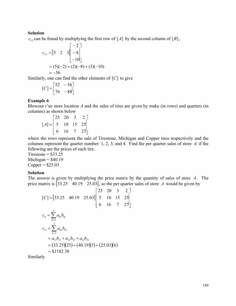
189

Solution

12c can be found by multiplying the first row of ][A by the second column of ][B ,

10

8

2

32512c

)10)(3()8)(2()2)(5( 56

Similarly, one can find the other elements of ][C to give

8876

5652][C

Example 6 Blowout r’us store location A and the sales of tires are given by make (in rows) and quarters (in columns) as shown below

277166

2515105

232025

][A

where the rows represent the sale of Tirestone, Michigan and Copper tires respectively and the columns represent the quarter number: 1, 2, 3, and 4. Find the per quarter sales of store A if the following are the prices of each tire. Tirestone = $33.25 Michigan = $40.19 Copper = $25.03

Solution The answer is given by multiplying the price matrix by the quantity of sales of store A . The price matrix is 03.2519.4025.33 , so the per quarter sales of store A would be given by

277166

2515105

232025

03.2519.4025.33][C

3

1kkjikij bac

3

11111

kkkbac

311321121111 bababa

603.25519.402525.33 38.1182$

Similarly

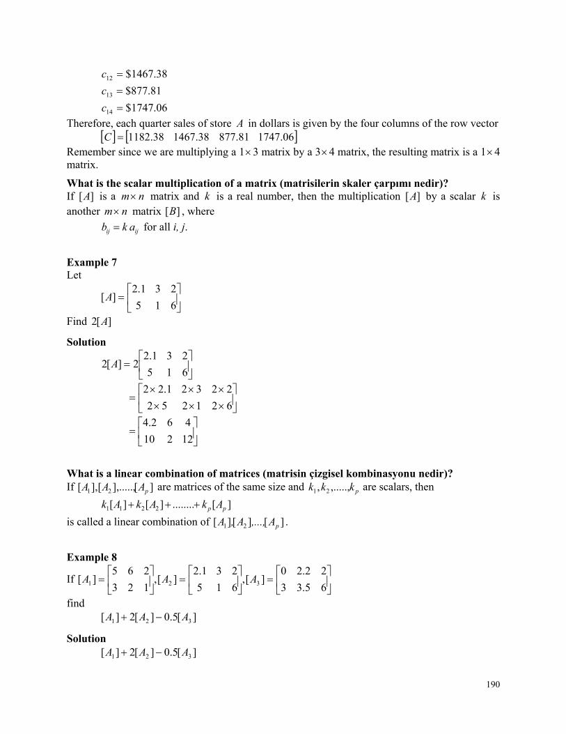
190

06.1747$

81.877$

38.1467$

14

13

12

c

c

c

Therefore, each quarter sales of store A in dollars is given by the four columns of the row vector 06.174781.87738.146738.1182C

Remember since we are multiplying a 13 matrix by a 34 matrix, the resulting matrix is a 14 matrix.

What is the scalar multiplication of a matrix (matrisilerin skaler çarpımı nedir)? If ][A is a nm matrix and k is a real number, then the multiplication ][A by a scalar k is another nm matrix ][B , where

ijij akb for all i, j.

Example 7 Let

615

231.2][A

Find ][2 A

Solution

615

231.22][2 A

621252

22321.22

12210

462.4

What is a linear combination of matrices (matrisin çizgisel kombinasyonu nedir)? If ][],.....,[],[ 21 pAAA are matrices of the same size and pkkk ,.....,, 21 are scalars, then

][........][][ 2211 pp AkAkAk

is called a linear combination of ][][][ 21 pA,...,A,A .

Example 8

If

65.33

22.20][,

615

231.2][,

123

265][ 321 AAA

find ][5.0][2][ 321 AAA

Solution ][5.0][2][ 321 AAA

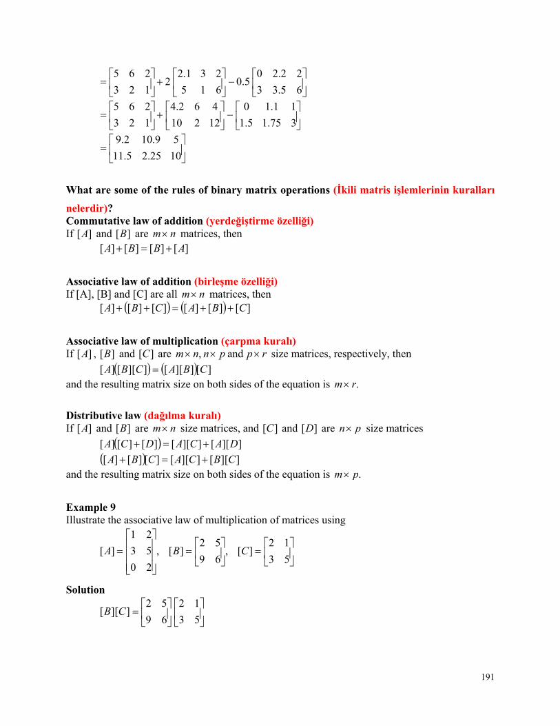
191

65.33

22.205.0

615

231.22

123

265

375.15.1

11.10

12210

462.4

123

265

1025.25.11

59.102.9

What are some of the rules of binary matrix operations (İkili matris işlemlerinin kuralları

nelerdir)? Commutative law of addition (yerdeğiştirme özelliği) If ][A and ][B are nm matrices, then

][][][][ ABBA

Associative law of addition (birleşme özelliği) If [A], [B] and [C] are all nm matrices, then

][][][][][][ CBACBA

Associative law of multiplication (çarpma kuralı) If ][A , ][B and ][C are rppnnm and , size matrices, respectively, then

][]][[]][[][ CBACBA and the resulting matrix size on both sides of the equation is .rm

Distributive law (dağılma kuralı) If ][A and ][B are nm size matrices, and ][C and ][D are pn size matrices

]][[]][[][][][ DACADCA

]][[]][[][][][ CBCACBA and the resulting matrix size on both sides of the equation is .pm

Example 9 Illustrate the associative law of multiplication of matrices using

53

12][,

69

52][,

20

53

21

][ CBA

Solution

]][[ CB

53

12

69

52

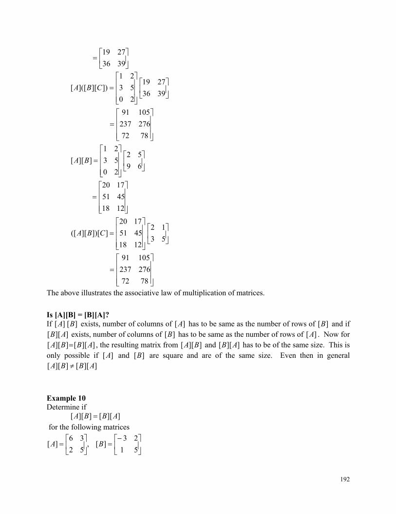
192

3936

2719

3936

2719

20

53

21

])][]([[ CBA

7872

276237

10591

69

52

20

53

21

]][[ BA

1218

4551

1720

53

12

1218

4551

1720

]])[][([ CBA

7872

276237

10591

The above illustrates the associative law of multiplication of matrices.

Is [A][B] = [B][A]? If ][A ][B exists, number of columns of ][A has to be same as the number of rows of ][B and if

]][[ AB exists, number of columns of ][B has to be same as the number of rows of ][A . Now for ]][[]][[ ABBA , the resulting matrix from ]][[ BA and ]][[ AB has to be of the same size. This is

only possible if ][A and ][B are square and are of the same size. Even then in general ]][[]][[ ABBA

Example 10 Determine if

]][[]][[ ABBA

for the following matrices

51

23][,

52

36][ BA

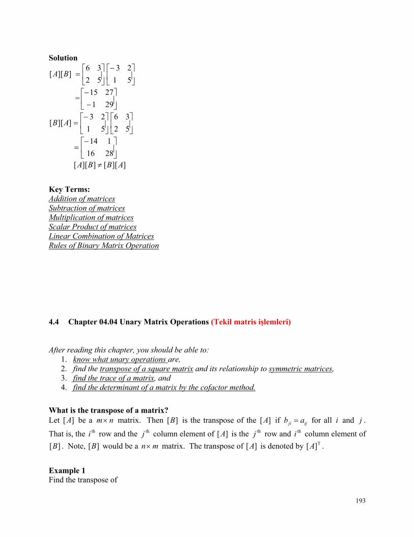
193

Solution

]][[ BA

51

23

52

36

=

291

2715

]][[ AB

52

36

51

23

2816

114

]][[]][[ ABBA

Key Terms: Addition of matrices Subtraction of matrices Multiplication of matrices Scalar Product of matrices Linear Combination of Matrices Rules of Binary Matrix Operation 4.4 Chapter 04.04 Unary Matrix Operations (Tekil matris işlemleri) After reading this chapter, you should be able to:

1. know what unary operations are, 2. find the transpose of a square matrix and its relationship to symmetric matrices, 3. find the trace of a matrix, and 4. find the determinant of a matrix by the cofactor method.

What is the transpose of a matrix? Let ][A be a nm matrix. Then ][B is the transpose of the ][A if ijji ab for all i and j .

That is, the thi row and the thj column element of ][A is the thj row and thi column element of

][B . Note, ][B would be a mn matrix. The transpose of ][A is denoted by T][A .

Example 1 Find the transpose of

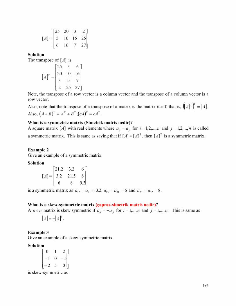
194

277166

2515105

232025

][A

Solution The transpose of ][A is

27252

7153

161020

6525

TA

Note, the transpose of a row vector is a column vector and the transpose of a column vector is a row vector.

Also, note that the transpose of a transpose of a matrix is the matrix itself, that is, AA TT .

Also, TTTTT ; cAcABABA .

What is a symmetric matrix (Simetrik matris nedir)? A square matrix ][A with real elements where jiij aa for ni ,...,2,1 and nj ,...,2,1 is called

a symmetric matrix. This is same as saying that if T][][ AA , then T][A is a symmetric matrix.

Example 2 Give an example of a symmetric matrix.

Solution

3.986

85.212.3

62.32.21

][A

is a symmetric matrix as 623 31132112 a, a.aa and 83223 aa .

What is a skew-symmetric matrix (çapraz-simetrik matris nedir)? A nn matrix is skew symmetric if jiij aa for ni ,...,1 and nj ,...,1 . This is same as

.TAA

Example 3 Give an example of a skew-symmetric matrix.

Solution

052

501

210

is skew-symmetric as

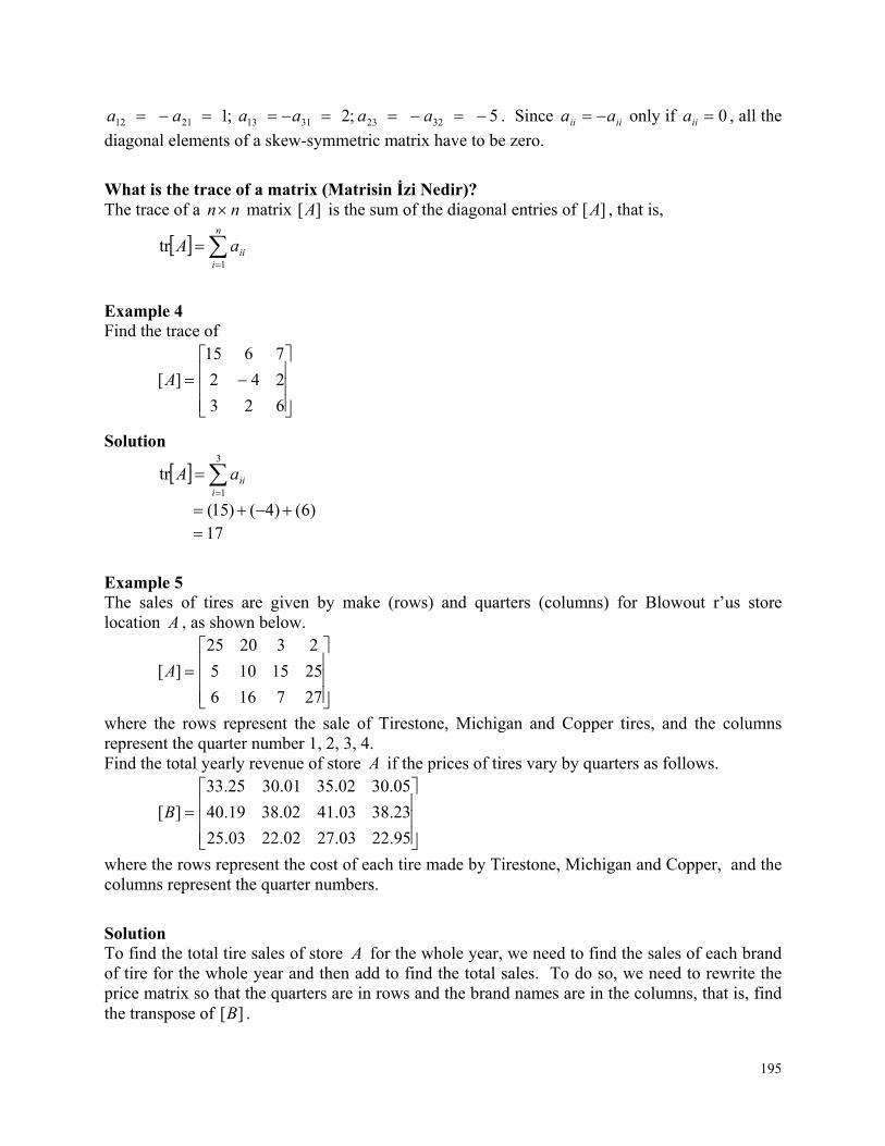
195

5 ;2;1 322331132112 a a a a a a . Since iiii aa only if 0iia , all the

diagonal elements of a skew-symmetric matrix have to be zero.

What is the trace of a matrix (Matrisin İzi Nedir)? The trace of a nn matrix ][A is the sum of the diagonal entries of ][A , that is,

n

iiiaA

1

tr

Example 4 Find the trace of

623

242

7615

][A

Solution

3

1

tri

iiaA

)6()4()15( 17

Example 5 The sales of tires are given by make (rows) and quarters (columns) for Blowout r’us store location A , as shown below.

277166

2515105

232025

][A

where the rows represent the sale of Tirestone, Michigan and Copper tires, and the columns represent the quarter number 1, 2, 3, 4. Find the total yearly revenue of store A if the prices of tires vary by quarters as follows.

95.2203.2702.2203.25

23.3803.4102.3819.40

05.3002.3501.3025.33

][B

where the rows represent the cost of each tire made by Tirestone, Michigan and Copper, and the columns represent the quarter numbers.

Solution To find the total tire sales of store A for the whole year, we need to find the sales of each brand of tire for the whole year and then add to find the total sales. To do so, we need to rewrite the price matrix so that the quarters are in rows and the brand names are in the columns, that is, find the transpose of ][B .

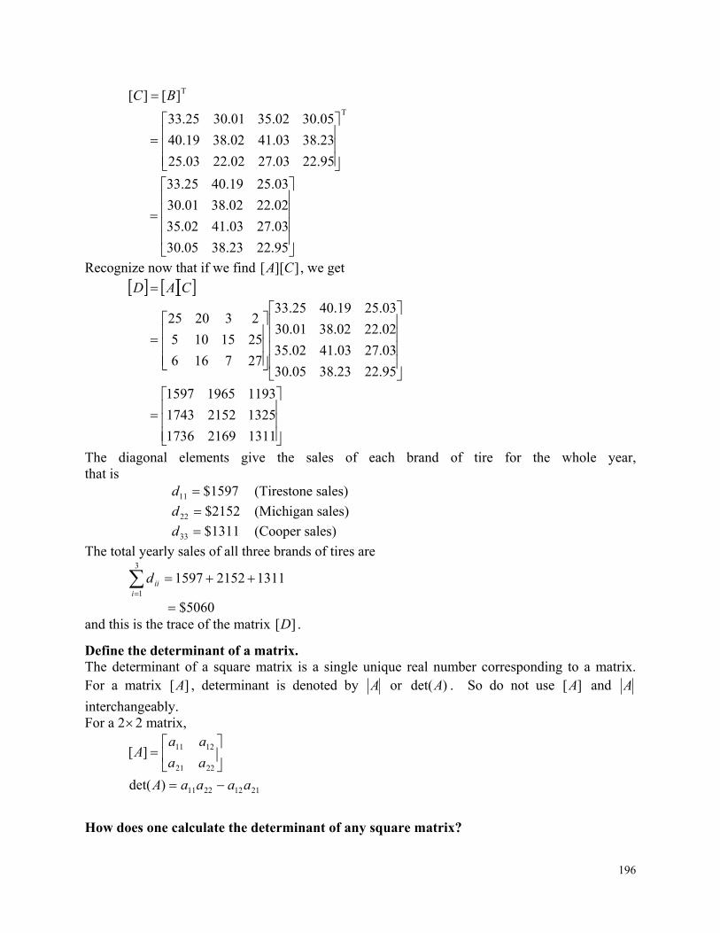
196

T][][ BC

T

95.2203.2702.2203.25

23.3803.4102.3819.40

05.3002.3501.3025.33

95.2223.3805.30

03.2703.4102.35

02.2202.3801.30

03.2519.4025.33

Recognize now that if we find ]][[ CA , we get

CAD

95.2223.3805.30

03.2703.4102.35

02.2202.3801.30

03.2519.4025.33

277166

2515105

232025

131121691736

132521521743

119319651597

The diagonal elements give the sales of each brand of tire for the whole year, that is 1597$11 d (Tirestone sales)

2152$22 d (Michigan sales)

1311$33 d (Cooper sales)

The total yearly sales of all three brands of tires are

1311215215973

1

i

iid

5060$ and this is the trace of the matrix ][D .

Define the determinant of a matrix. The determinant of a square matrix is a single unique real number corresponding to a matrix. For a matrix ][A , determinant is denoted by A or )det(A . So do not use ][A and A

interchangeably. For a 22 matrix,

2221

1211][aa

aaA

21122211)det( aaaaA

How does one calculate the determinant of any square matrix?

197

Let ][A be nn matrix. The minor of entry ija is denoted by ijM and is defined as the

determinant of the )1(1( nn submatrix of ][A , where the submatrix is obtained by deleting

the thi row and thj column of the matrix ][A . The determinant is then given by

n

jijij

ji niMaA1

,,2,1anyfor1det

or

n

iijij

ji njMaA1

,,2,1anyfor1det

Coupled that with ][matrix11afordet 11 AaA , we can always reduce the determinant of a

matrix to determinants of 11 matrices. The number ijji M )1( is called the cofactor of ija and

is denoted by ijc . The formula for the determinant can then be written as

n

jijij niCaA

1

,,2,1anyfordet

or

n

iijij njCaA

1

,,2,1anyfordet

Determinants are not generally calculated using this method as it becomes computationally intensive for large matrices. For a nn matrix, it requires arithmetic operations proportional to n!.

Example 6 Find the determinant of

112144

1864

1525

][A

Solution

Method 1:

3

1

3,2,1anyfor1detj

ijijji iMaA

Let us choose 1i in the formula

3

111

11detj

jjj MaA

131331

121221

111111 111 MaMaMa

131312121111 MaMaMa

198

112

1811 M

4

1144

16412 M

80

12144

86413 M

384

131312121111)det( MaMaMaA

3841805425 384400100 84 Also for 1i ,

3

111det

jjjCaA

1111

11 1 MC

11M 4

1221

12 1 MC

12M 80

1331

13 1 MC

13M

384 313121211111det CaCaCaA

384)1(80)5(4)25( 384400100 84

Method 2:

3

1

1deti

ijijji MaA for any 3,2,1j

Let us choose 2j in the formula

3

122

21deti

iii MaA

323223

222222

121221 111 MaMaMa

323222221212 MaMaMa

199

1144

16412 M

80

1144

12522 M

119

164

12532 M

39

323222221212)det( MaMaMaA

)39(12)119(8)80(5 468952400 84

In terms of cofactors for 2j ,

3

122det

iii CaA

1221

12 1 MC

12M 80

2222

22 1 MC

22M 119

3223

32 1 MC

32M

39 323222221212det CaCaCaA

39)12(119)8(80)5( 468952400 84

Is there a relationship between det(AB), and det(A) and det(B)? Yes, if ][A and ][B are square matrices of same size, then

)det()det()det( BAAB

Are there some other theorems that are important in finding the determinant of a square

matrix? Theorem 1: If a row or a column in a nn matrix ][A is zero, then 0)det( A . Theorem 2: Let ][A be a nn matrix. If a row is proportional to another row, then 0)det( A .

200

Theorem 3: Let ][A be a nn matrix. If a column is proportional to another column, then 0)det( A .

Theorem 4: Let ][A be a nn matrix. If a column or row is multiplied by k to result in matrix k , then )det()det( AkB .

Theorem 5: Let ][A be a nn upper or lower triangular matrix, then ii

n

iaA

1)det(

.

Example 7 What is the determinant of

1250

5940

4730

3620

][A

Solution Since one of the columns (first column in the above example) of ][A is a zero, 0)det( A .

Example 8 What is the determinant of

18359

10245

6723

4612

][A

Solution )det(A is zero because the fourth column

18

10

6

4

is 2 times the first column

9

5

3

2

Example 9 If the determinant of

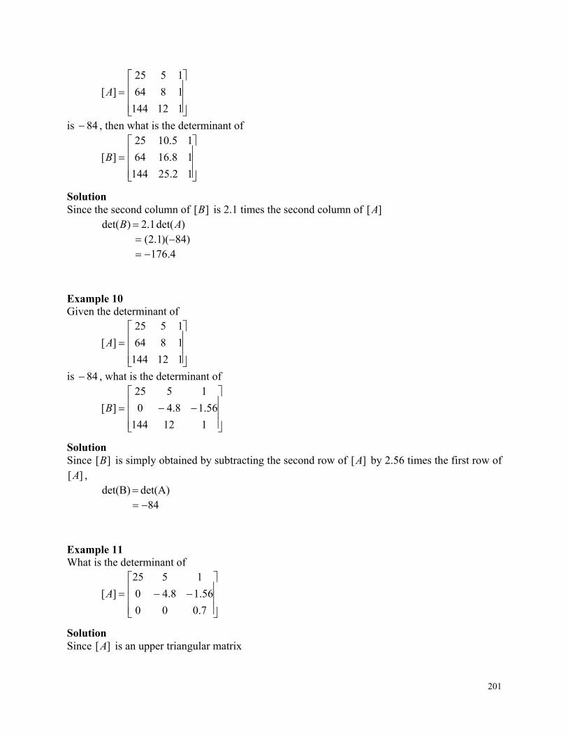
201

112144

1864

1525

][A

is 84 , then what is the determinant of

12.25144

18.1664

15.1025

][B

Solution Since the second column of ][B is 2.1 times the second column of ][A

)det( 2.1 )det( AB )84)(1.2(

176.4

Example 10 Given the determinant of

112144

1864

1525

][A

is 84 , what is the determinant of

112144

56.18.40

1525

][B

Solution Since ][B is simply obtained by subtracting the second row of ][A by 2.56 times the first row of

][A , det(A) det(B)

84

Example 11 What is the determinant of

7.000

56.18.40

1525

][A

Solution Since ][A is an upper triangular matrix

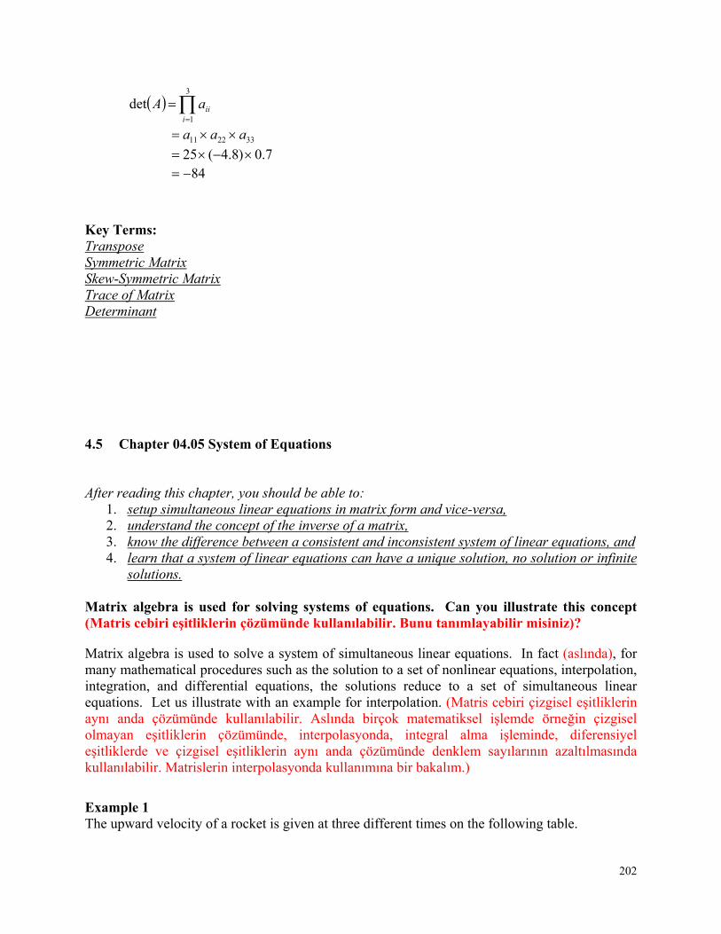
202

3

1

deti

iiaA

332211 aaa

7.0)8.4(25 84

Key Terms: Transpose Symmetric Matrix Skew-Symmetric Matrix Trace of Matrix Determinant 4.5 Chapter 04.05 System of Equations After reading this chapter, you should be able to:

1. setup simultaneous linear equations in matrix form and vice-versa, 2. understand the concept of the inverse of a matrix, 3. know the difference between a consistent and inconsistent system of linear equations, and 4. learn that a system of linear equations can have a unique solution, no solution or infinite

solutions. Matrix algebra is used for solving systems of equations. Can you illustrate this concept (Matris cebiri eşitliklerin çözümünde kullanılabilir. Bunu tanımlayabilir misiniz)?

Matrix algebra is used to solve a system of simultaneous linear equations. In fact (aslında), for many mathematical procedures such as the solution to a set of nonlinear equations, interpolation, integration, and differential equations, the solutions reduce to a set of simultaneous linear equations. Let us illustrate with an example for interpolation. (Matris cebiri çizgisel eşitliklerin aynı anda çözümünde kullanılabilir. Aslında birçok matematiksel işlemde örneğin çizgisel olmayan eşitliklerin çözümünde, interpolasyonda, integral alma işleminde, diferensiyel eşitliklerde ve çizgisel eşitliklerin aynı anda çözümünde denklem sayılarının azaltılmasında kullanılabilir. Matrislerin interpolasyonda kullanımına bir bakalım.)

Example 1 The upward velocity of a rocket is given at three different times on the following table.

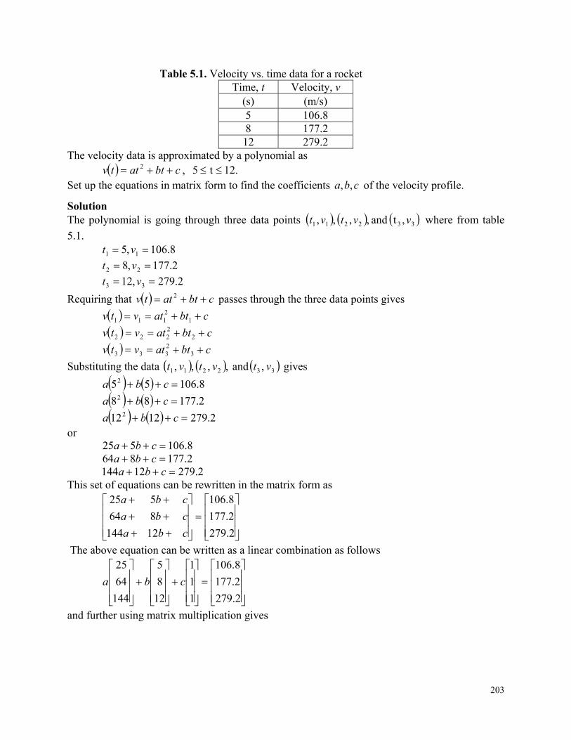
203

Table 5.1. Velocity vs. time data for a rocket Time, t Velocity, v

(s) (m/s) 5 106.8 8 177.2 12 279.2

The velocity data is approximated by a polynomial as 12.t5 , 2 cbtattv

Set up the equations in matrix form to find the coefficients cba ,, of the velocity profile.

Solution The polynomial is going through three data points 332211 ,t and ,, ,, vvtvt where from table

5.1. 8.106,5 11 vt

2.177,8 22 vt

2.279,12 33 vt

Requiring that cbtattv 2 passes through the three data points gives

cbtatvtv 12111

cbtatvtv 22222

cbtatvtv 32333

Substituting the data 332211 ,and , , , , vtvtvt gives

8.106552 cba

2.177882 cba

2.27912122 cba or

8.106525 cba 2.177864 cba

2.27912144 cba This set of equations can be rewritten in the matrix form as

2.279

2.177

8.106

12144

864

525

cba

cba

cba

The above equation can be written as a linear combination as follows

2.279

2.177

8.106

1

1

1

12

8

5

144

64

25

cba

and further using matrix multiplication gives

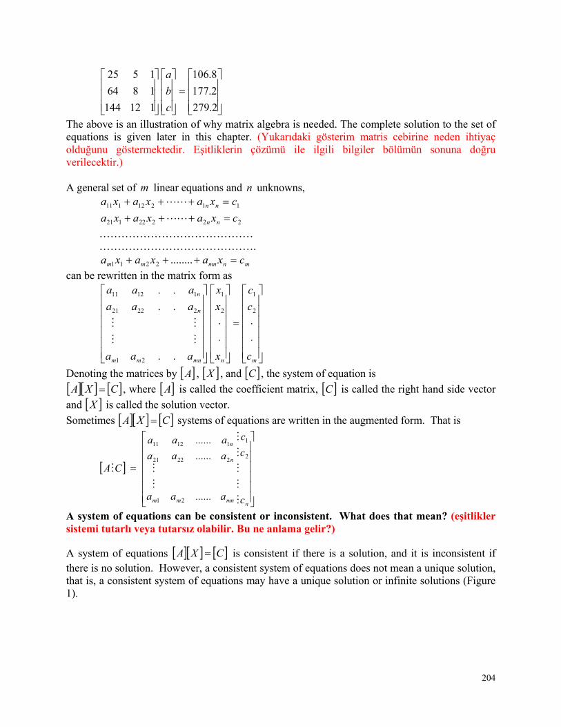
204

2.279

2.177

8.106

112144

1864

1525

c

b

a

The above is an illustration of why matrix algebra is needed. The complete solution to the set of equations is given later in this chapter. (Yukarıdaki gösterim matris cebirine neden ihtiyaç olduğunu göstermektedir. Eşitliklerin çözümü ile ilgili bilgiler bölümün sonuna doğru verilecektir.) A general set of m linear equations and n unknowns,

11212111 cxaxaxa nn

22222121 cxaxaxa nn

…………………………………… …………………………………….

mnmnmm cxaxaxa ........2211

can be rewritten in the matrix form as

mnmnmm

n

n

c

c

c

x

x

x

aaa

aaa

aaa

2

1

2

1

21

22221

11211

..

..

..

Denoting the matrices by A , X , and C , the system of equation is

CXA , where A is called the coefficient matrix, C is called the right hand side vector

and X is called the solution vector.

Sometimes CXA systems of equations are written in the augmented form. That is

nmnmm

n

n

c

c

c

a......aa

a......aa

a......aa

CA2

1

21

22221

11211

A system of equations can be consistent or inconsistent. What does that mean? (eşitlikler sistemi tutarlı veya tutarsız olabilir. Bu ne anlama gelir?)

A system of equations CXA is consistent if there is a solution, and it is inconsistent if there is no solution. However, a consistent system of equations does not mean a unique solution, that is, a consistent system of equations may have a unique solution or infinite solutions (Figure 1).

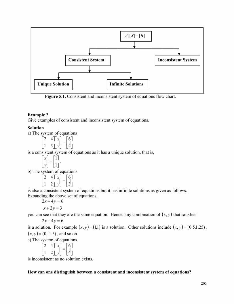
205

Figure 5.1. Consistent and inconsistent system of equations flow chart.

Example 2 Give examples of consistent and inconsistent system of equations.

Solution a) The system of equations

4

6

31

42

y

x

is a consistent system of equations as it has a unique solution, that is,

1

1

y

x.

b) The system of equations

3

6

21

42

y

x

is also a consistent system of equations but it has infinite solutions as given as follows. Expanding the above set of equations,

32

642

yx

yx

you can see that they are the same equation. Hence, any combination of yx, that satisfies 642 yx

is a solution. For example 1,1, yx is a solution. Other solutions include )25.1,5.0(, yx ,

)5.1 ,0(, yx , and so on. c) The system of equations

4

6

21

42

y

x

is inconsistent as no solution exists.

How can one distinguish between a consistent and inconsistent system of equations?

Consistent System Inconsistent System

Unique Solution Infinite Solutions

[A][X]= [B]

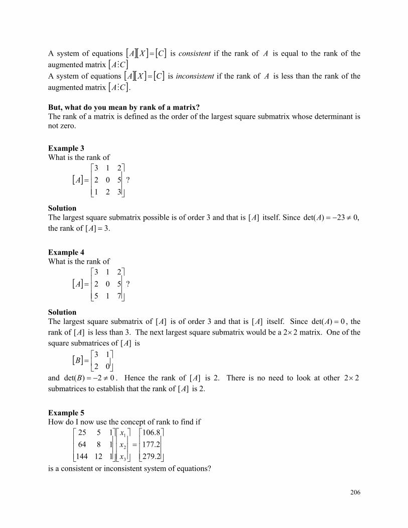
206

A system of equations CXA is consistent if the rank of A is equal to the rank of the

augmented matrix CA

A system of equations CXA is inconsistent if the rank of A is less than the rank of the

augmented matrix CA . But, what do you mean by rank of a matrix? The rank of a matrix is defined as the order of the largest square submatrix whose determinant is not zero.

Example 3 What is the rank of

321

502

213

A ?

Solution The largest square submatrix possible is of order 3 and that is ][A itself. Since ,023)det( A the rank of .3][ A

Example 4 What is the rank of

715

502

213

A ?

Solution The largest square submatrix of ][A is of order 3 and that is ][A itself. Since 0)det( A , the rank of ][A is less than 3. The next largest square submatrix would be a 22 matrix. One of the square submatrices of ][A is

02

13B

and 02)det( B . Hence the rank of ][A is 2. There is no need to look at other 22 submatrices to establish that the rank of ][A is 2.

Example 5 How do I now use the concept of rank to find if

2.279

2.177

8.106

112144

1864

1525

3

2

1

x

x

x

is a consistent or inconsistent system of equations?

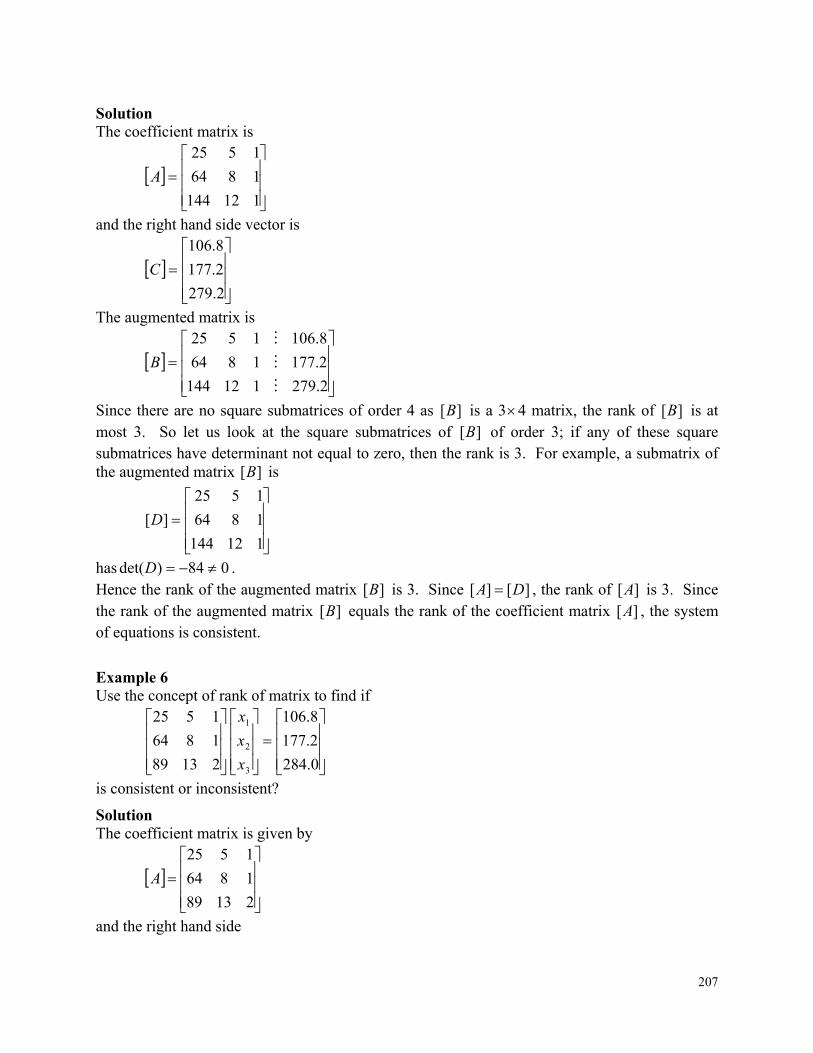
207

Solution The coefficient matrix is

112144

1864

1525

A

and the right hand side vector is

2.279

2.177

8.106

C

The augmented matrix is

2.279112144

2.1771864

8.1061525

B

Since there are no square submatrices of order 4 as ][B is a 34 matrix, the rank of ][B is at most 3. So let us look at the square submatrices of ][B of order 3; if any of these square submatrices have determinant not equal to zero, then the rank is 3. For example, a submatrix of the augmented matrix ][B is

112144

1864

1525

][D

has 084)det( D . Hence the rank of the augmented matrix ][B is 3. Since ][][ DA , the rank of ][A is 3. Since the rank of the augmented matrix ][B equals the rank of the coefficient matrix ][A , the system of equations is consistent.

Example 6 Use the concept of rank of matrix to find if

0.284

2.177

8.106

21389

1864

1525

3

2

1

x

x

x

is consistent or inconsistent?

Solution The coefficient matrix is given by

21389

1864

1525

A

and the right hand side

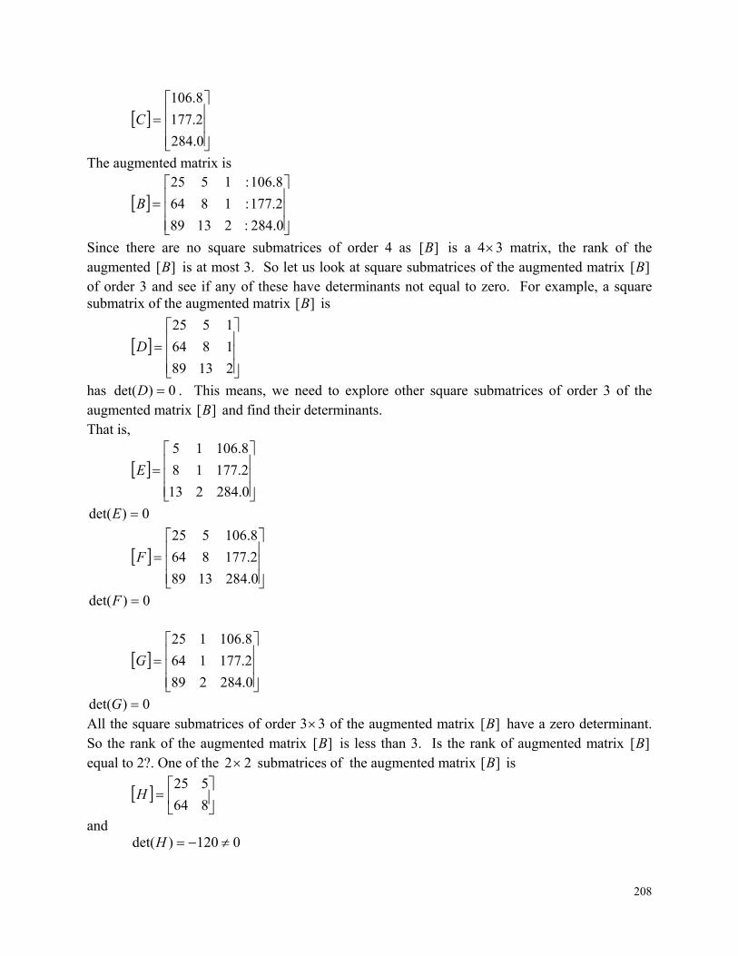
208

0.284

2.177

8.106

C

The augmented matrix is

0.284:21389

2.177:1864

8.106:1525

B

Since there are no square submatrices of order 4 as ][B is a 43 matrix, the rank of the augmented ][B is at most 3. So let us look at square submatrices of the augmented matrix ][B of order 3 and see if any of these have determinants not equal to zero. For example, a square submatrix of the augmented matrix ][B is

21389

1864

1525

D

has 0)det( D . This means, we need to explore other square submatrices of order 3 of the augmented matrix ][B and find their determinants. That is,

0.284213

2.17718

8.10615

E

0)det( E

0.2841389

2.177864

8.106525

F

0)det( F

0.284289

2.177164

8.106125

G

0)det( G All the square submatrices of order 33 of the augmented matrix ][B have a zero determinant. So the rank of the augmented matrix ][B is less than 3. Is the rank of augmented matrix ][B equal to 2?. One of the 22 submatrices of the augmented matrix ][B is

864

525H

and 0120)det( H

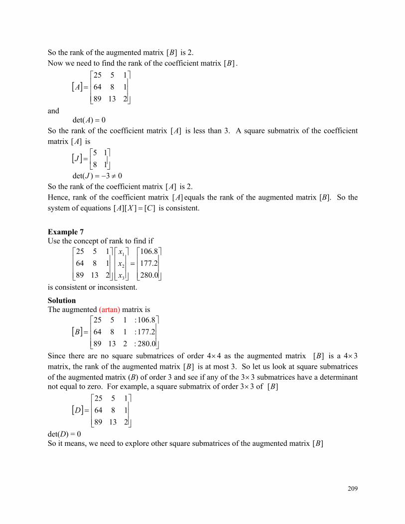
209

So the rank of the augmented matrix ][B is 2. Now we need to find the rank of the coefficient matrix ][B .

21389

1864

1525

A

and 0)det( A

So the rank of the coefficient matrix ][A is less than 3. A square submatrix of the coefficient matrix ][A is

18

15J

03)det( J So the rank of the coefficient matrix ][A is 2. Hence, rank of the coefficient matrix ][A equals the rank of the augmented matrix [B]. So the system of equations ][][][ CXA is consistent.

Example 7 Use the concept of rank to find if

0.280

2.177

8.106

21389

1864

1525

3

2

1

x

x

x

is consistent or inconsistent.

Solution The augmented (artan) matrix is

0.280:21389

2.177:1864

8.106:1525

B

Since there are no square submatrices of order 44 as the augmented matrix ][B is a 43 matrix, the rank of the augmented matrix ][B is at most 3. So let us look at square submatrices of the augmented matrix (B) of order 3 and see if any of the 33 submatrices have a determinant not equal to zero. For example, a square submatrix of order 33 of ][B

21389

1864

1525

D

det(D) = 0 So it means, we need to explore other square submatrices of the augmented matrix ][B

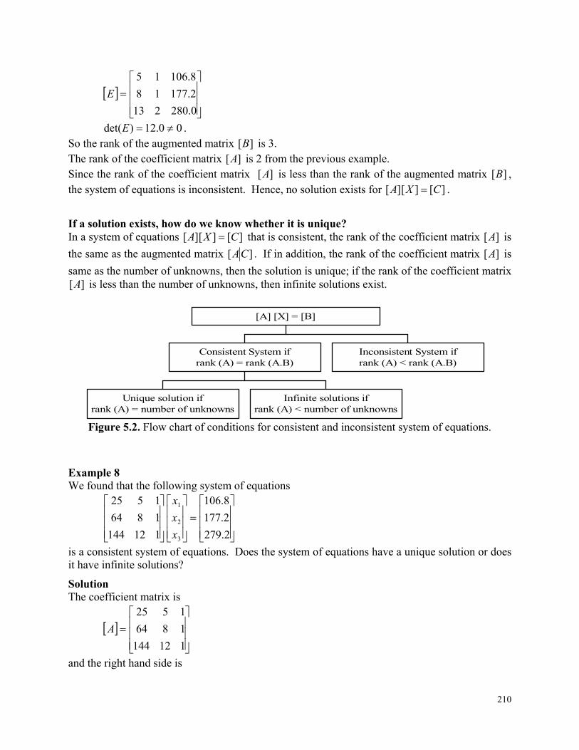
210

0.280213

2.17718

8.10615

E

00.12)det( E . So the rank of the augmented matrix ][B is 3. The rank of the coefficient matrix ][A is 2 from the previous example. Since the rank of the coefficient matrix ][A is less than the rank of the augmented matrix ][B , the system of equations is inconsistent. Hence, no solution exists for ][][][ CXA .

If a solution exists, how do we know whether it is unique? In a system of equations ][][][ CXA that is consistent, the rank of the coefficient matrix ][A is

the same as the augmented matrix ][ CA . If in addition, the rank of the coefficient matrix ][A is

same as the number of unknowns, then the solution is unique; if the rank of the coefficient matrix ][A is less than the number of unknowns, then infinite solutions exist.

Unique solution ifrank (A) = number of unknowns

Infinite solutions ifrank (A) < number of unknowns

Consistent System ifrank (A) = rank (A.B)

Inconsistent System ifrank (A) < rank (A.B)

[A] [X] = [B]

Figure 5.2. Flow chart of conditions for consistent and inconsistent system of equations.

Example 8 We found that the following system of equations

2.279

2.177

8.106

112144

1864

1525

3

2

1

x

x

x

is a consistent system of equations. Does the system of equations have a unique solution or does it have infinite solutions?

Solution The coefficient matrix is

112144

1864

1525

A

and the right hand side is

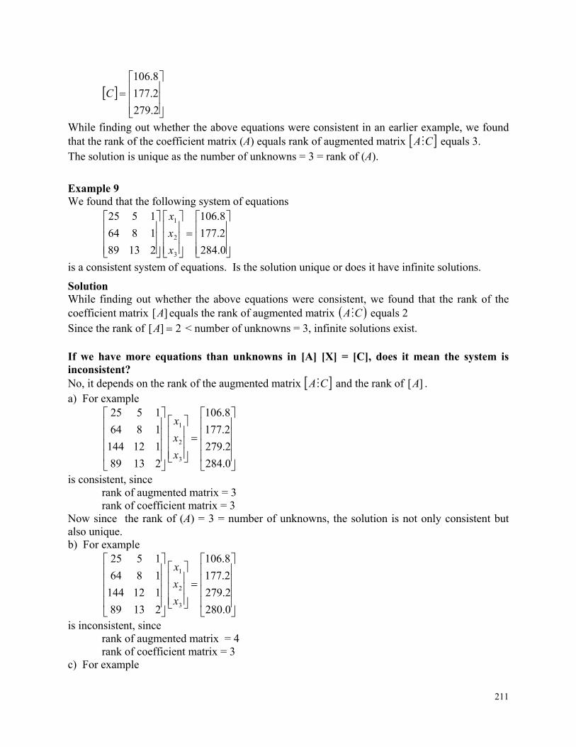
211

2.279

2.177

8.106

C

While finding out whether the above equations were consistent in an earlier example, we found that the rank of the coefficient matrix (A) equals rank of augmented matrix CA equals 3. The solution is unique as the number of unknowns = 3 = rank of (A).

Example 9 We found that the following system of equations

0.284

2.177

8.106

21389

1864

1525

3

2

1

x

x

x

is a consistent system of equations. Is the solution unique or does it have infinite solutions.

Solution While finding out whether the above equations were consistent, we found that the rank of the coefficient matrix ][A equals the rank of augmented matrix CA equals 2 Since the rank of 2][ A < number of unknowns = 3, infinite solutions exist. If we have more equations than unknowns in [A] [X] = [C], does it mean the system is inconsistent? No, it depends on the rank of the augmented matrix CA and the rank of ][A . a) For example

0.284

2.279

2.177

8.106

21389

112144

1864

1525

3

2

1

x

x

x

is consistent, since rank of augmented matrix = 3 rank of coefficient matrix = 3

Now since the rank of (A) = 3 = number of unknowns, the solution is not only consistent but also unique. b) For example

0.280

2.279

2.177

8.106

21389

112144

1864

1525

3

2

1

x

x

x

is inconsistent, since rank of augmented matrix = 4 rank of coefficient matrix = 3

c) For example

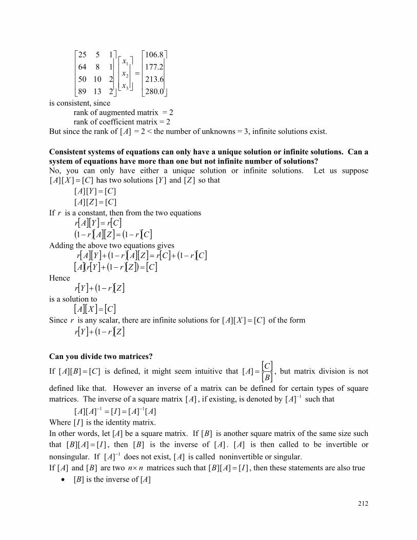
212

0.280

6.213

2.177

8.106

21389

21050

1864

1525

3

2

1

x

x

x

is consistent, since rank of augmented matrix = 2 rank of coefficient matrix = 2

But since the rank of ][A = 2 < the number of unknowns = 3, infinite solutions exist. Consistent systems of equations can only have a unique solution or infinite solutions. Can a system of equations have more than one but not infinite number of solutions? No, you can only have either a unique solution or infinite solutions. Let us suppose

][][ ][ CXA has two solutions ][Y and ][Z so that ][][ ][ CYA ][][ ][ CZA

If r is a constant, then from the two equations CrYAr

CrZAr 1 1 Adding the above two equations gives

CrCrZArYAr 1 1

CZrYrA 1 Hence

ZrYr 1 is a solution to

CXA Since r is any scalar, there are infinite solutions for ][][][ CXA of the form

ZrYr 1

Can you divide two matrices?

If ][][][ CBA is defined, it might seem intuitive that B

CA ][ , but matrix division is not

defined like that. However an inverse of a matrix can be defined for certain types of square matrices. The inverse of a square matrix ][A , if existing, is denoted by 1][ A such that

][][][][][ 11 AAIAA Where ][I is the identity matrix. In other words, let [A] be a square matrix. If ][B is another square matrix of the same size such that ][][][ IAB , then ][B is the inverse of ][A . ][A is then called to be invertible or

nonsingular. If 1][ A does not exist, ][A is called noninvertible or singular. If ][A and ][B are two nn matrices such that ][][][ IAB , then these statements are also true

[B] is the inverse of [A]

213

[A] is the inverse of [B] [A] and [B] are both invertible [A] [B]=[I]. [A] and [B] are both nonsingular all columns of [A] and [B]are linearly independent all rows of [A] and [B] are linearly independent.

Example 10 Determine if

35

23][B

is the inverse of

35

23[A]

Solution

]][[ AB

35

23

35

23

10

01

][I Since ][][][ IAB ,

][B is the inverse of [A] and ][A is the inverse of ][B . But, we can also show that

]][[ BA

35

23

35

23

10

01

I][ to show that ][A is the inverse of ][B .

Can I use the concept of the inverse of a matrix to find the solution of a set of equations [A]

[X] = [C]? Yes, if the number of equations is the same as the number of unknowns, the coefficient matrix

][A is a square matrix. Given

][][][ CXA

Then, if 1][ A exists, multiplying both sides by 1][ A .

][][]][[][ 11 CAXAA

214

][][][][ 1 CAXI

][][][ 1 CAX

This implies that if we are able to find 1][ A , the solution vector of ][][][ CXA is simply a

multiplication of 1][ A and the right hand side vector, ][C .

How do I find the inverse of a matrix? If ][A is a nn matrix, then 1][ A is a nn matrix and according to the definition of inverse of a matrix

][][][ 1 IAA Denoting

nnnn

n

n

aaa

aaa

aaa

A

21

22221

11211

][

''2

'1

'2

'22

'21

'1

'12

'11

1][

nnnn

n

n

aaa

aaa

aaa

A

10

1

0

010

001

][I

Using the definition of matrix multiplication, the first column of the 1][ A matrix can then be found by solving

0

0

1

'1

'21

'11

21

22221

11211

nnnnn

n

n

a

a

a

aaa

aaa

aaa

Similarly, one can find the other columns of the 1][ A matrix by changing the right hand side accordingly.

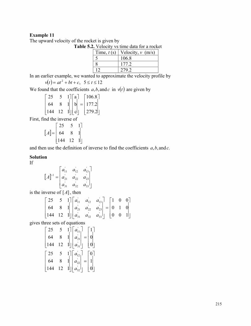
215

Example 11 The upward velocity of the rocket is given by

Table 5.2. Velocity vs time data for a rocket Time, t (s) Velocity, v (m/s) 5 106.8 8 177.2 12 279.2

In an earlier example, we wanted to approximate the velocity profile by 125 ,2 tcbtattv

We found that the coefficients cba and,, in tv are given by

2.279

2.177

8.106

c

b

a

112144

1864

1525

First, find the inverse of

112144

1864

1525

A

and then use the definition of inverse to find the coefficients .and,, cba

Solution If

'33

'32

'31

'23

'22

'21

'13

'12

'11

1

aaa

aaa

aaa

A

is the inverse of ][A , then

100

010

001

112144

1864

1525

'33

'32

'31

'23

'22

'21

'13

'12

'11

aaa

aaa

aaa

gives three sets of equations

0

0

1

112144

1864

1525

'31

'21

'11

a

a

a

0

1

0

112144

1864

1525

'32

'22

'12

a

a

a

216

1

0

0

112144

1864

1525

'33

'23

'13

a

a

a

Solving the above three sets of equations separately gives

'31

'21

'11

a

a

a

=

571.4

9524.0

04762.0

'32

'22

'12

a

a

a

=

000.5

417.1

08333.0

429.1

4643.0

03571.0

'33

'23

'13

a

a

a

Hence

429.1000.5571.4

4643.0417.19524.0

03571.008333.004762.0

][ 1A

Now CXA

where

c

b

a

X

2.279

2.177

8.106

C

Using the definition of ,1A

11 CAXAA

CA X 1

2.279

2.177

8.106

429.1000.5571.4

4643.0417.19524.0

03571.008333.004762.0

Hence

217

086.1

69.19

2905.0

c

b

a

So 125 ,086.169.192905.0 2 ttttv

Is there another way to find the inverse of a matrix? For finding the inverse of small matrices, the inverse of an invertible matrix can be found by

AadjA

Adet

11

where

T

21

22221

11211

nnnn

n

n

CCC

CCC

CCC

Aadj

where ijC are the cofactors of ija . The matrix

nnn

n

n

CC

CCC

CCC

1

22221

11211

itself is called the matrix of cofactors from [A]. Cofactors are defined in Chapter 4.

Example 12 Find the inverse of

112144

1864

1525

A

Solution From Example 4.6 in Chapter 04.06, we found

84det A Next we need to find the adjoint of ][A . The cofactors of A are found as follows.

The minor of entry 11a is

112144

1864

1525

11 M

112

18

218

4 The cofactors of entry 11a is

1111

11 1 MC

11M 4 The minor of entry 12a is

112144

1864

1525

12 M

1144

164

80 The cofactor of entry 12a is

1221

12 1 MC

12M )80( 80 Similarly 38413 C

721 C

11922 C

42023 C

331 C

3932 C

12033 C

Hence the matrix of cofactors of ][A is

120393

4201197

384804

C

The adjoint of matrix ][A is T][C ,

TCAadj

120420384

3911980

374

Hence

AadjA

Adet

11

219

120420384

3911980

374

84

1

429.1000.5571.4

4643.0417.19524.0

03571.008333.004762.0

If the inverse of a square matrix [A] exists, is it unique? ( bir kare [A] matrisinin tersi varsa denklem sistemininçözümü de var mıdır? ) Yes, the inverse of a square matrix is unique, if it exists. The proof is as follows. Assume that the inverse of ][A is ][B and if this inverse is not unique, then let another inverse of ][A exist called ][C . If ][B is the inverse of ][A , then

][][][ IAB Multiply both sides by ][C ,

][][][][][ CICAB ][][][][ CCAB

Since [C] is inverse of ][A , ][][][ ICA

Multiply both sides by ][B , ][][][ CIB

][][ CB This shows that ][B and ][C are the same. So the inverse of ][A is unique.

Key Terms: Consistent system Inconsistent system Infinite solutions Unique solution Rank Inverse 4.5.1 Multiple-Choice Test Chapter 04.01 Background Simultaneous Linear Equations

1. Given A =

6000

5400

3210

9326

then A is a (an) ______________ matrix.

220

(A) diagonal (B) identity (C) lower triangular (D) upper triangular 2. A square matrix A is lower triangular if

(A) ijaij ,0 (B) jiaij ,0 (C) jiaij ,0 (D) ijaij ,0

3. Given

3.123.113.10

3.113.103.11

3.203.123.12

][A ,

2011

65

42

][B

then if BAC , then

31c _____________________

(A) 2.58 (B) 6.37 (C) 219.4 (D) 259.4

4. The following system of equations has ____________ solution(s). 2 yx (x=0, y=2; x=1, y=1; x=2, y=0; x=4, y=-2, x=6, y=-4...) 1266 yx

(A) infinite (B) no (C) two (D) unique 5. Consider there are only two computer companies in a country. The companies are named

Dude and Imac. Each year, Dude keeps 1/5th of its customers, while the rest switch to Imac. Each year, Imac keeps 1/3rd of its customers, while the rest switch to Dude. If in 2003, Dude had 1/6th of the market and Imac had 5/6th of the market, what will be the share of Dude computers when the market becomes stable? (bir şehirde 2 bilgisayar şirketinin olduğunu kabul edelim. Bu şirketlerin adları Dude ve Imac olsun. Dude şirketi her yıl müşterilerinin 1/5’ni korumakta, geri kalanlar Imac’i tercih etmektedir. Imac firması ise her yıl müşterilerinin 1/3’nü koruyabilmekte geri kalan müşteriler Dude şirketini tercih etmektedir. 2003 yılında Dude pazarın 1/6’sına sahipken Imac 5/6’sına hakimdir. Pazar kararlı hale geldiğinde Dude şirketinin payı aşağıdakilerden hangisi olabilir?)

(A) 37/90 (B) 5/11 (C) 6/11 (D) 53/90 6. Three kids - Jim, Corey and David receive an inheritance of $2,253,453. The money is

put in three trusts but is not divided equally to begin with. Corey's trust is three times that of David's because Corey made an A in Dr. Kaw’s class. Each trust is put in an interest generating investment. The three trusts of Jim, Corey and David pays an interest of 6%, 8%, 11%, respectively. The total interest of all the three trusts combined at the end of the first year is $190,740.57. The equations to find the trust money of Jim ( J ), Corey (C ) and David ( D ) in a matrix form is (Jim, Corey ve David 2,253,453$’lık mirasa konmuşlardır. Para, çocuklar arasında eşit paylaştırılmamaktadır. Corey Kaw’ın dersinden A notunu aldığı için David’in payının 3 katı kadar para almaktadır. Her pay

221

faiz veren bir şirkete yatırılmıştır. Bu şirket Jim’e %6, Corey’e %8, ve David’e 11 kar vermektedir. )

(A)

57.740,190

0

453,253,2

11.008.006.0

130

111

D

C

J

(B)

57.740,190

0

453,253,2

11.008.006.0

310

111

D

C

J

(C)

57.740,190

0

453,253,2

1186

310

111

D

C

J

(D)

057,074,19

0

453,253,2

1186

130

111

D

C

J

For a complete solution, refer to the links at the end of the book. 4.6 Chapter 04.06 Gaussian Elimination (Gauss eleme yöntemi)

PRE-REQUISITES

1. Matrix Algebra Basics: Binary operations on matrices and inverse of a matrix (Primer for Matrix Algebra).

OBJECTIVES 1. solve a set of simultaneous linear equations using Naïve Gauss elimination (basit Gauss

eleme), 2. learn the pitfalls of the Naïve Gauss elimination method (Gauss eleme yönteminde

düşülen hatalar), 3. understand the effect of round-off error when solving a set of linear equations with the

Naïve Gauss elimination method (basit Gauss eleme yöntemi ile çizgisel denklemler çözülürken yuvarlama hatalarının etkisinin belirlenmesi),

4. learn how to modify the Naïve Gauss elimination method to the Gaussian elimination with partial pivoting method to avoid pitfalls of the former method (basit Gauss eleme yönteminin kısmen pivotlamalı Gauss eleme yöntemine dönüştürülmesi),

5. find the determinant of a square matrix using Gaussian elimination, and (Gauss eleme yönteminde kullanılacak olan kare matrisin determinantının hesaplanması)

6. understand the relationship between the determinant of a coefficient matrix and the solution of simultaneous linear equations (katsayılar matrisinin determinantının ve çizgisel eşitliklerin aynı anda çözümü arasındaki ilişkinin anlaşılması).

After reading this chapter, you should be able to:

1. solve a set of simultaneous linear equations using Naïve Gauss elimination, 2. learn the pitfalls of the Naïve Gauss elimination method, 3. understand the effect of round-off error when solving a set of linear equations with the

Naïve Gauss elimination method, 4. learn how to modify the Naïve Gauss elimination method to the Gaussian elimination

with partial pivoting method to avoid pitfalls of the former method,

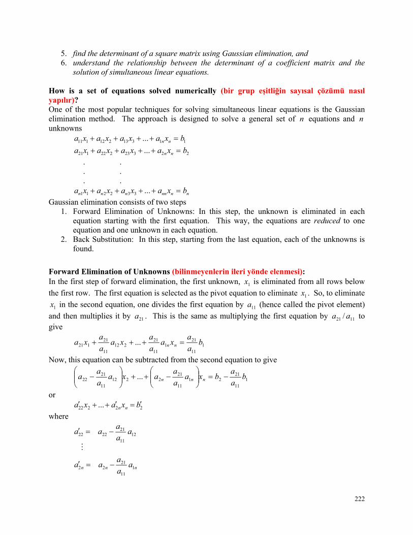
222

5. find the determinant of a square matrix using Gaussian elimination, and 6. understand the relationship between the determinant of a coefficient matrix and the

solution of simultaneous linear equations. How is a set of equations solved numerically (bir grup eşitliğin sayısal çözümü nasıl yapılır)? One of the most popular techniques for solving simultaneous linear equations is the Gaussian elimination method. The approach is designed to solve a general set of n equations and n unknowns

11313212111 ... bxaxaxaxa nn

22323222121 ... bxaxaxaxa nn

. . . . . .

nnnnnnn bxaxaxaxa ...332211

Gaussian elimination consists of two steps 1. Forward Elimination of Unknowns: In this step, the unknown is eliminated in each

equation starting with the first equation. This way, the equations are reduced to one equation and one unknown in each equation.

2. Back Substitution: In this step, starting from the last equation, each of the unknowns is found.

Forward Elimination of Unknowns (bilinmeyenlerin ileri yönde elenmesi): In the first step of forward elimination, the first unknown, 1x is eliminated from all rows below

the first row. The first equation is selected as the pivot equation to eliminate 1x . So, to eliminate

1x in the second equation, one divides the first equation by 11a (hence called the pivot element)

and then multiplies it by 21a . This is the same as multiplying the first equation by 1121 / aa to give

111

211

11

21212

11

21121 ... b

a

axa

a

axa

a

axa nn

Now, this equation can be subtracted from the second equation to give

111

2121

11

212212

11

2122 ... b

a

abxa

a

aaxa

a

aa nnn

or

22222 ... bxaxa nn

where

nnn aa

aaa

aa

aaa

111

2122

1211

212222

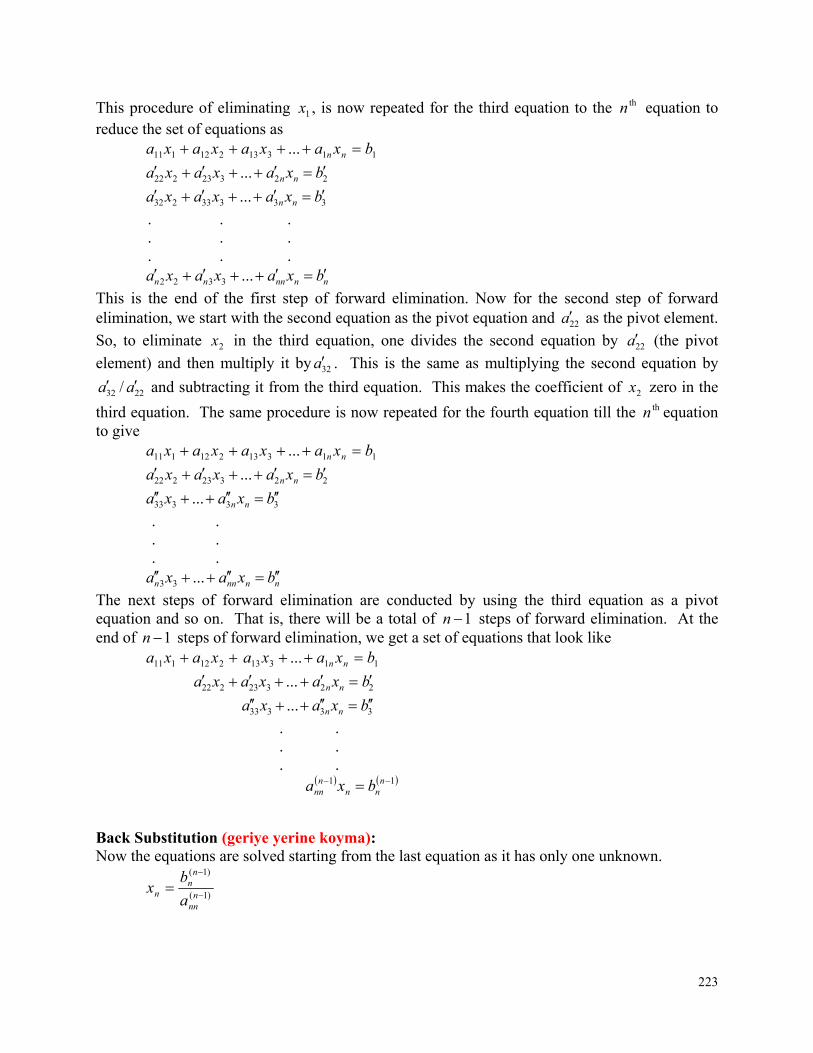
223

This procedure of eliminating 1x , is now repeated for the third equation to the thn equation to reduce the set of equations as

11313212111 ... bxaxaxaxa nn

22323222 ... bxaxaxa nn

33333232 ... bxaxaxa nn

. . . . . . . . .

nnnnnn bxaxaxa ...3322

This is the end of the first step of forward elimination. Now for the second step of forward elimination, we start with the second equation as the pivot equation and 22a as the pivot element.

So, to eliminate 2x in the third equation, one divides the second equation by 22a (the pivot

element) and then multiply it by 32a . This is the same as multiplying the second equation by

2232 / aa and subtracting it from the third equation. This makes the coefficient of 2x zero in the

third equation. The same procedure is now repeated for the fourth equation till the thn equation to give

11313212111 ... bxaxaxaxa nn

22323222 ... bxaxaxa nn

33333 ... bxaxa nn

. . . . . .

nnnnn bxaxa ...33

The next steps of forward elimination are conducted by using the third equation as a pivot equation and so on. That is, there will be a total of 1n steps of forward elimination. At the end of 1n steps of forward elimination, we get a set of equations that look like

212111 xaxa 11313 ... bxaxa nn

22323222 ... bxaxaxa nn

33333 ... bxaxa nn

. . . . . . 11 n

nnn

nn bxa

Back Substitution (geriye yerine koyma): Now the equations are solved starting from the last equation as it has only one unknown.

)1(

)1(

n

nn

nn

n a

bx

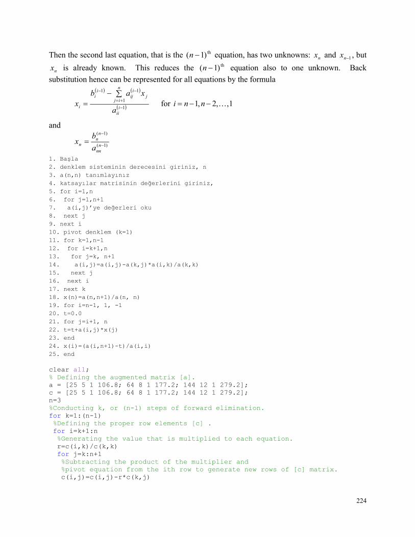
224

Then the second last equation, that is the th)1( n equation, has two unknowns: nx and 1nx , but

nx is already known. This reduces the th)1( n equation also to one unknown. Back

substitution hence can be represented for all equations by the formula

1

1

11

iii

n

ijj

iij

ii

i a

xabx for 1,,2,1 nni

and

)1(

)1(

n

nn

nn

n a

bx

1. Başla 2. denklem sisteminin derecesini giriniz, n 3. a(n,n) tanımlayınız 4. katsayılar matrisinin değerlerini giriniz, 5. for i=1,n 6. for j=1,n+1 7. a(i,j)’ye değerleri oku 8. next j 9. next i 10. pivot denklem (k=1) 11. for k=1,n-1 12. for i=k+1,n 13. for j=k, n+1 14. a(i,j)=a(i,j)-a(k,j)*a(i,k)/a(k,k) 15. next j 16. next i 17. next k 18. x(n)=a(n,n+1)/a(n, n) 19. for i=n-1, 1, -1 20. t=0.0 21. for j=i+1, n 22. t=t+a(i,j)*x(j) 23. end 24. x(i)=(a(i,n+1)-t)/a(i,i) 25. end clear all; % Defining the augmented matrix [a]. a = [25 5 1 106.8; 64 8 1 177.2; 144 12 1 279.2]; c = [25 5 1 106.8; 64 8 1 177.2; 144 12 1 279.2]; n=3 %Conducting k, or (n-1) steps of forward elimination. for k=1:(n-1) %Defining the proper row elements [c] . for i=k+1:n %Generating the value that is multiplied to each equation. r=c(i,k)/c(k,k) for j=k:n+1 %Subtracting the product of the multiplier and %pivot equation from the ith row to generate new rows of [c] matrix. c(i,j)=c(i,j)-r*c(k,j)

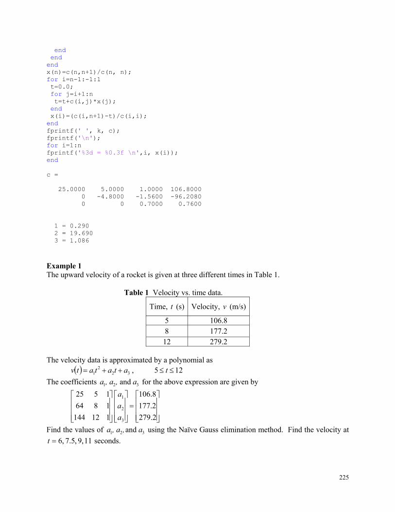
225

end end end x(n)=c(n,n+1)/c(n, n); for i=n-1:-1:1 t=0.0; for j=i+1:n t=t+c(i,j)*x(j); end x(i)=(c(i,n+1)-t)/c(i,i); end fprintf(' ', k, c); fprintf('\n'); for i=1:n fprintf('%3d = %0.3f \n',i, x(i)); end c = 25.0000 5.0000 1.0000 106.8000 0 -4.8000 -1.5600 -96.2080 0 0 0.7000 0.7600 1 = 0.290 2 = 19.690 3 = 1.086

Example 1 The upward velocity of a rocket is given at three different times in Table 1.

Table 1 Velocity vs. time data.

Time, t (s) Velocity, v (m/s)

5 106.8 8 177.2 12 279.2

The velocity data is approximated by a polynomial as

125 , 322

1 tatatatv

The coefficients 321 and a, , aa for the above expression are given by

2.279

2.177

8.106

112144

1864

1525

3

2

1

a

a

a

Find the values of 321 and a,, aa using the Naïve Gauss elimination method. Find the velocity at

11 ,9 ,5.7 ,6t seconds.

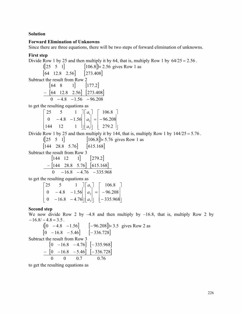
226

Solution

Forward Elimination of Unknowns Since there are three equations, there will be two steps of forward elimination of unknowns.

First step Divide Row 1 by 25 and then multiply it by 64, that is, multiply Row 1 by 2.5664/25 .

56.28.106 1525 gives Row 1 as

408.27356.28.1264 Subtract the result from Row 2

208.9656.18.40

408.27356.28.1264

2.1771 864

to get the resulting equations as

2.279

208.96

8.106

112144

56.18.40

1525

3

2

1

a

a

a

Divide Row 1 by 25 and then multiply it by 144, that is, multiply Row 1 by 5.76144/25 . 76.58.106 1525 gives Row 1 as

168.61576.58.28144 Subtract the result from Row 3

968.33576.48.16 0

168.61576.58.28144

2.2791 12144

to get the resulting equations as

968.335

208.96

8.106

76.48.160

56.18.40

1525

3

2

1

a

a

a

Second step We now divide Row 2 by –4.8 and then multiply by –16.8, that is, multiply Row 2 by

3.54.816.8/ . 5.3208.96 56.18.40 gives Row 2 as

728.33646.58.160 Subtract the result from Row 3

76.0 7.0 0 0

728.33646.58.160

968.3354.768.160

to get the resulting equations as

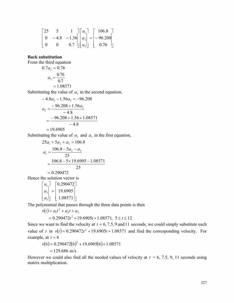
227

76.0

208.96

8.106

7.000

56.18.40

1525

3

2

1

a

a

a

Back substitution From the third equation

76.07.0 3 a

70

760 3 .

.a

1.08571 Substituting the value of 3a in the second equation,

208.9656.18.4 32 aa

8.4

56.1208.96 32

aa

4.8

08571.11.5696.208

690519. Substituting the value of 2a and 3a in the first equation,

8.106525 321 aaa

25

58.106 32

1

aaa

25

08571.16905.1958.106

290472.0 Hence the solution vector is

08571.1

6905.19

290472.0

3

2

1

a

a

a

The polynomial that passes through the three data points is then 32

21 atatatv

125 ,08571.16905.19290472.0 2 ttt Since we want to find the velocity at 11 and 9 ,5.7 ,6t seconds, we could simply substitute each

value of t in 08571.16905.19290472.0 2 tttv and find the corresponding velocity. For example, at 6t

m/s686.129

08571.166905.196290472.06 2

v

However we could also find all the needed values of velocity at t = 6, 7.5, 9, 11 seconds using matrix multiplication.

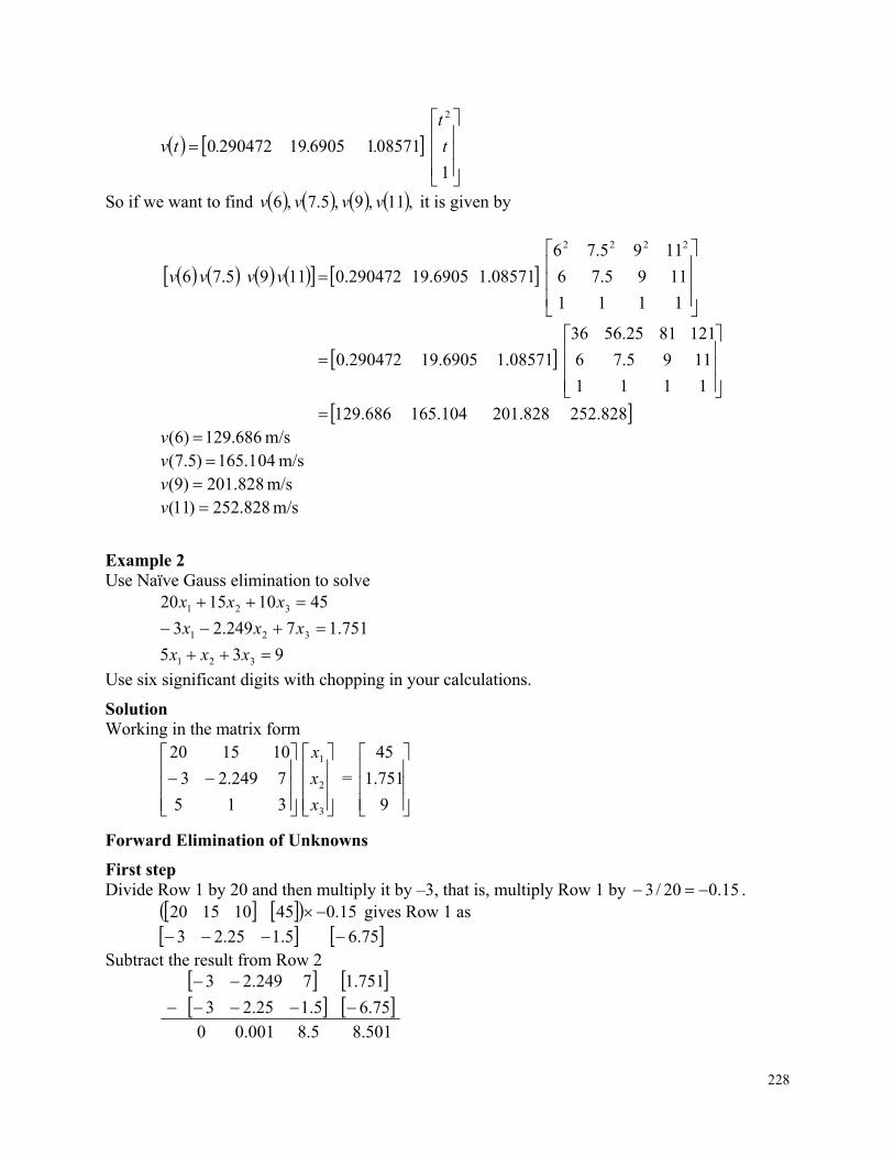
228

1

0857116905192904720

2

t

t

. . .tv

So if we want to find ,11 ,9 ,5.7 ,6 vvvv it is given by

1111

1195.76

1195.76

08571.1 6905.19 0.290472 11 9 5.7 6

2222

vvvv

1111

1197.56

1218156.2536

1.08571 19.6905 290472.0

252.828 201.828 165.104 686.129 m/s 686.129)6( v

m/s 041.165)5.7( v m/s 828.201)9( v m/s 828.252)11( v

Example 2 Use Naïve Gauss elimination to solve

45101520 321 xxx

751.17249.23 321 xxx

935 321 xxx

Use six significant digits with chopping in your calculations.

Solution Working in the matrix form

315

7249.23

101520

3

2

1

x

x

x

=

9

751.1

45

Forward Elimination of Unknowns

First step Divide Row 1 by 20 and then multiply it by –3, that is, multiply Row 1 by 15.020/3 .

15.045101520 gives Row 1 as

75.65.125.23 Subtract the result from Row 2

501.8 5.8 001.0 0

75.65.125.23

751.17 249.23

229

to get the resulting equations as

315

5.8001.00

101520

3

2

1

x

x

x

=

9

501.8

45

Divide Row 1 by 20 and then multiply it by 5, that is, multiply Row 1 by 25.020/5 25.045101520 gives Row 1 as

25.115.275.35 Subtract the result from Row 3

2.25 .5075.20

25.115.2 75.3 5

93 1 5

to get the resulting equations as

5.075.20

5.8001.00

101520

3

2

1

x

x

x

=

25.2

501.8

45

Second step Now for the second step of forward elimination, we will use Row 2 as the pivot equation and eliminate Row 3: Column 2. Divide Row 2 by 0.001 and then multiply it by –2.75, that is, multiply Row 2 by

2750001.0/75.2 . 2750501.85.8001.00 gives Row 2 as

75.233772337575.20 Rewriting within 6 significant digits with chopping

7.233772337575.20 Subtract the result from Row 3

3375.452 5.23375 0 0

7.2337723375 2.75 0

25.2.50 75.2 0

Rewriting within 6 significant digits with chopping 4.233755.2337500 to get the resulting equations as

5.2337500

5.8001.00

101520

3

2

1

x

x

x

=

4.23375

501.8

45

This is the end of the forward elimination steps.

Back substitution We can now solve the above equations by back substitution. From the third equation,

4.233755.23375 3 x

230

5.23375

4.233753 x

999995.0 Substituting the value of 3x in the second equation

501.85.8001.0 32 xx

0.001

0.999995585018

001.0

5.8501.8 32

..

xx

001.0

49995.8501.8

001.0

00105.0

05.1 Substituting the value of 3x and 2x in the first equation,

45101520 321 xxx

20

10 1545 321

xxx

20

999995.01005.11545

20

2500.1920

99995.925.2920

99995.975.1545

9625.0 Hence the solution is

3

2

1

][

x

x

x

X

999995.0

05.1

9625.0

Compare this with the exact solution of

3

2

1

x

x

x

X

231

1

1

1

Are there any pitfalls of the Naïve Gauss elimination method? (Yalın Gauss eleme yönteminde karşılaşılabilecek sıkıntılar/tuzaklar) Yes, there are two pitfalls of the Naïve Gauss elimination method. Division by zero: It is possible for division by zero to occur during the beginning of the 1n steps of forward elimination. For example

1165 32 xx

16754 321 xxx

15329 321 xxx

will result in division by zero in the first step of forward elimination as the coefficient of 1x in the first equation is zero as is evident when we write the equations in matrix form.

15

16

11

329

754

650

3

2

1

x

x

x

But what about the equations below: Is division by zero a problem? 18765 321 xxx

2531210 321 xxx

56191720 321 xxx

Written in matrix form,

56

25

18

191720

31210

765

3

2

1

x

x

x

there is no issue of division by zero in the first step of forward elimination. The pivot element is the coefficient of 1x in the first equation, 5, and that is a non-zero number. However, at the end of the first step of forward elimination, we get the following equations in matrix form (ileri yönde elemede sıfıra bölme sorunu yoktur. İlk eşitliğin pivot elemanı yani x1’in katsayısı 5’tir. Ancak ilk aşamanın sonunda aşağıdaki gibi bir matris elde edilir)

16

11

18

970

1100

765

3

2

1

x

x

x

Now at the beginning of the 2nd step of forward elimination, the coefficient of 2x in Equation 2 would be used as the pivot element. That element is zero and hence would create the division by zero problem. So it is important to consider that the possibility of division by zero can occur at the beginning of any step of forward elimination.

232

Round-off error: The Naïve Gauss elimination method is prone to round-off errors (basit Gauss eleme yöntemi yuvarlama hatasının oluşmasına eğilimlidir). This is true when there are large numbers of equations as errors propagate (bu durum büyük sayıda eşitliklerin olduğunda hata daha başat olmaktadır). Also, if there is subtraction of numbers from each other, it may create large errors. See the example below.

Example 3 Remember Example 2 where we used Naïve Gauss elimination to solve

45101520 321 xxx

751.17249.23 321 xxx

935 321 xxx

using six significant digits with chopping in your calculations? Repeat the problem, but now use five significant digits with chopping in your calculations.

Solution Writing in the matrix form

315

7249.23

101520

3

2

1

x

x

x

=

9

751.1

45

Forward Elimination of Unknowns (bilinmeyenlerin ileri yönde elenmesi)

First step Divide Row 1 by 20 and then multiply it by –3, that is, multiply Row 1 by 15.020/3 .

15.045101520 gives Row 1 as

75.65.125.23 Subtract the result from Row 2

501.8 5.8 001.0 0

75.65.125.23

751.17 249.23

to get the resulting equations as

315

5.8001.00

101520

3

2

1

x

x

x

=

9

501.8

45

Divide Row 1 by 20 and then multiply it by 5, that is, multiply Row 1 by 25.020/5 . 25.045101520 gives Row 1 as

25.115.275.35 Subtract the result from Row 3

2.25 .5075.20

25.115.2 75.3 5

93 1 5

to get the resulting equations as

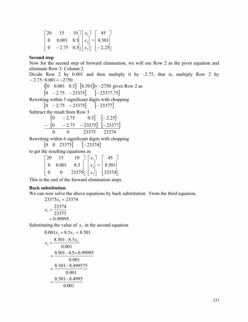
233

5.075.20

5.8001.00

101520

3

2

1

x

x

x

=

25.2

501.8

45

Second step Now for the second step of forward elimination, we will use Row 2 as the pivot equation and eliminate Row 3: Column 2. Divide Row 2 by 0.001 and then multiply it by –2.75, that is, multiply Row 2 by

2750001.0/75.2 . 2750501.85.8001.00 gives Row 2 as

75.233772337575.20 Rewriting within 5 significant digits with chopping

233772337575.20 Subtract the result from Row 3

33742 23375 0 0

2337723375 2.75 0

25.2.50 75.2 0

Rewriting within 6 significant digits with chopping 233742337500 to get the resulting equations as

2337500

5.8001.00

101520

3

2

1

x

x

x

=

23374

501.8

45

This is the end of the forward elimination steps.

Back substitution We can now solve the above equations by back substitution. From the third equation,

2337423375 3 x

23375

233743 x

99995.0 Substituting the value of 3x in the second equation

501.85.8001.0 32 xx

0.001

0.99995585018

001.0

5.8501.8 32

..

xx

001.0

4995.8501.8001.0

499575.8501.8

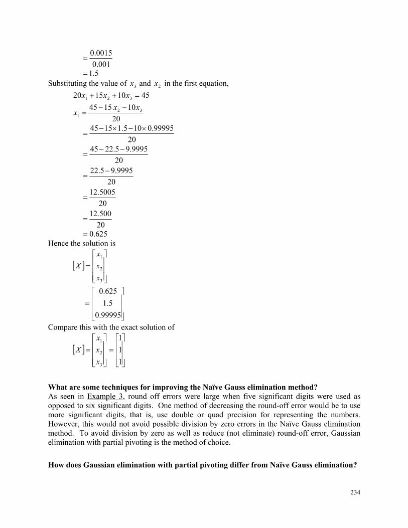
234

001.0

0015.0

5.1 Substituting the value of 3x and 2x in the first equation,

45101520 321 xxx

20

10 1545 321

xxx

20

99995.0105.11545

20

500.1220

5005.1220

9995.95.2220

9995.95.2245

625.0 Hence the solution is

3

2

1

x

x

x

X

99995.0

5.1

625.0

Compare this with the exact solution of

3

2

1

x

x

x

X

1

1

1

What are some techniques for improving the Naïve Gauss elimination method? As seen in Example 3, round off errors were large when five significant digits were used as opposed to six significant digits. One method of decreasing the round-off error would be to use more significant digits, that is, use double or quad precision for representing the numbers. However, this would not avoid possible division by zero errors in the Naïve Gauss elimination method. To avoid division by zero as well as reduce (not eliminate) round-off error, Gaussian elimination with partial pivoting is the method of choice.

How does Gaussian elimination with partial pivoting differ from Naïve Gauss elimination?

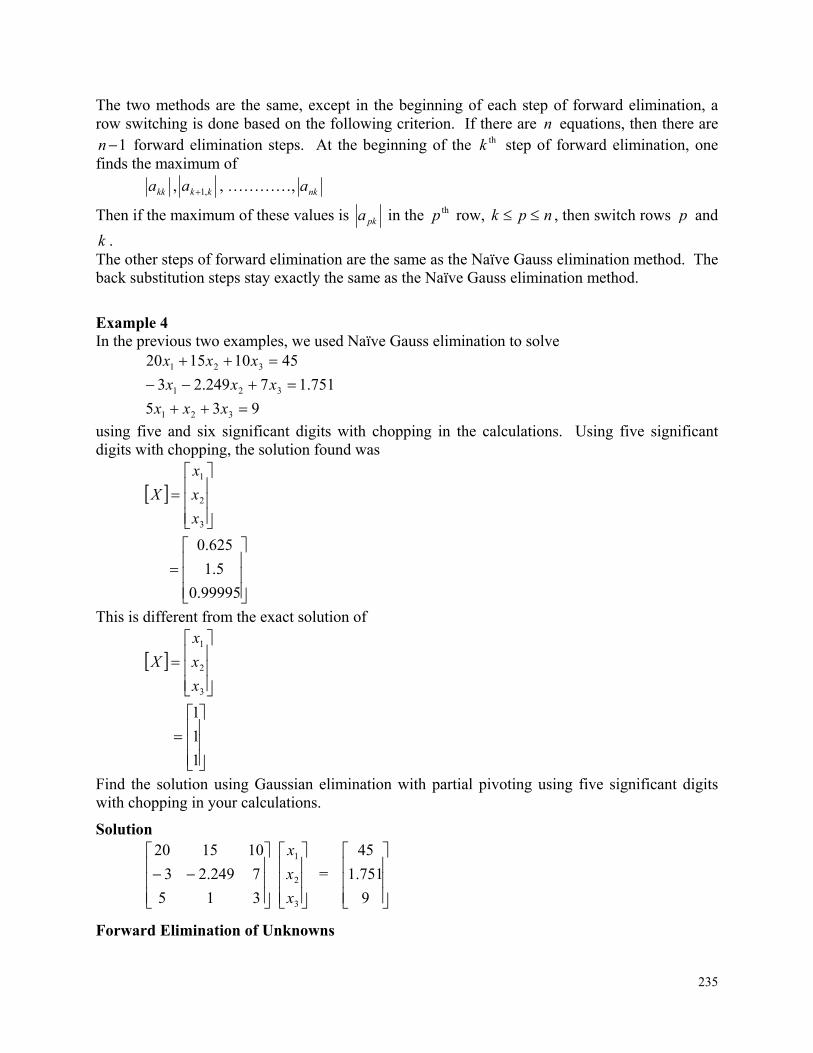
235

The two methods are the same, except in the beginning of each step of forward elimination, a row switching is done based on the following criterion. If there are n equations, then there are

1n forward elimination steps. At the beginning of the thk step of forward elimination, one finds the maximum of

kka , kka ,1 , …………, nka

Then if the maximum of these values is pka in the thp row, npk , then switch rows p and

k . The other steps of forward elimination are the same as the Naïve Gauss elimination method. The back substitution steps stay exactly the same as the Naïve Gauss elimination method.

Example 4 In the previous two examples, we used Naïve Gauss elimination to solve

45101520 321 xxx

751.17249.23 321 xxx

935 321 xxx

using five and six significant digits with chopping in the calculations. Using five significant digits with chopping, the solution found was

3

2

1

x

x

x

X

99995.0

5.1

625.0

This is different from the exact solution of

3

2

1

x

x

x

X

1

1

1

Find the solution using Gaussian elimination with partial pivoting using five significant digits with chopping in your calculations.

Solution

315

7249.23

101520

3

2

1

x

x

x

=

9

751.1

45

Forward Elimination of Unknowns

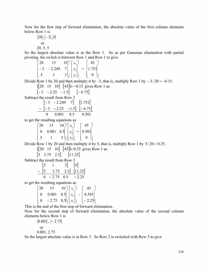
236

Now for the first step of forward elimination, the absolute value of the first column elements below Row 1 is

20 , 3 , 5

or 20, 3, 5

So the largest absolute value is in the Row 1. So as per Gaussian elimination with partial pivoting, the switch is between Row 1 and Row 1 to give

315

7249.23

101520

3

2

1

x

x

x

=

9

751.1

45

Divide Row 1 by 20 and then multiply it by –3, that is, multiply Row 1 by 15.020/3 . 15.045101520 gives Row 1 as

75.65.125.23 Subtract the result from Row 2

501.8 5.8 001.0 0

75.65.125.23

751.17 249.23

to get the resulting equations as

315

5.8001.00

101520

3

2

1

x

x

x

=

9

501.8

45

Divide Row 1 by 20 and then multiply it by 5, that is, multiply Row 1 by 25.020/5 . 25.045101520 gives Row 1 as

25.115.275.35 Subtract the result from Row 3

2.25 .5075.20

25.115.2 75.3 5

93 1 5

to get the resulting equations as

5.075.20

5.8001.00

101520

3

2

1

x

x

x

=

25.2

501.8

45

This is the end of the first step of forward elimination. Now for the second step of forward elimination, the absolute value of the second column elements below Row 1 is

001.0 , 75.2

or 0.001, 2.75

So the largest absolute value is in Row 3. So Row 2 is switched with Row 3 to give

237

5.8001.00

5.075.20

101520

3

2

1

x

x

x

=

501.8

25.2

45

Divide Row 2 by –2.75 and then multiply it by 0.001, that is, multiply Row 2 by 00036363.075.2/001.0 .

00036363.025.25.075.20 gives Row 2 as

00081816.000018182.000099998.00 Subtract the result from Row 3

.500181848 50018182.8 0 0

00081816.00.00018182 .000999980 0

501.8.58 .0010 0

Rewriting within 5 significant digits with chopping 5001.85001.800

to get the resulting equations as

5001.800

5.075.20

101520

3

2

1

x

x

x

=

5001.8

25.2

45

Back substitution 5001.85001.8 3 x

5001.8

5001.83 x

=1 Substituting the value of 3x in Row 2

25.25.075.2 32 xx

75.2

5.025.2 22

xx

75.2

15.025.2

75.2

5.025.2

75.2

75.2

1 Substituting the value of 3x and 2x in Row 1

45101520 321 xxx

20

101545 321

xxx

20

11011545

238

20

1030

20

101545

20

20

1 So the solution is

3

2

1

x

x

x

X

=

1

1

1

This, in fact, is the exact solution. By coincidence only, in this case, the round-off error is fully removed.

Can we use Naïve Gauss elimination methods to find the determinant of a square matrix? One of the more efficient ways to find the determinant of a square matrix is by taking advantage of the following two theorems on a determinant of matrices coupled with Naïve Gauss elimination.

Theorem 1: Let ][A be a nn matrix. Then, if ][B is a nn matrix that results from adding or subtracting a multiple of one row to another row, then )det()det( BA (The same is true for column operations also). [A]’nın nxn şeklinde bir matris oldupunu kabul edelim. [B] matrisinin’de nxn şeklinde bir matris olduğunu kabul edelim ve bir satırının diğer satırı ile toplandığında veya çıkarıldığında det(A)=det(B) şeklinde bir sonuç veribilir.

Theorem 2: Let ][A be a nn matrix that is upper triangular, lower triangular or diagonal, then

nnii aaaaA ......)det( 2211

n

iiia

1

This implies that if we apply the forward elimination steps of the Naïve Gauss elimination method, the determinant of the matrix stays the same according to Theorem 1. Then since at the end of the forward elimination steps, the resulting matrix is upper triangular, the determinant will be given by Theorem 2. [A]’nın nxn şeklinde üst üçgen, alt üçgen veya diyagonal bir matris olduğunu kabul edelim. Bu durumda det(A)=a11xa22xa33x…xann = aii

239

ifadesi yazılabilir. Bunun anlamı denklem sisteminin çözümü için basit gauss eleme yöntemi kullanılıyorsa matrisin determinantının Teorem 1’e göre aynı kalacağını göstermektedir.

Example 5 Find the determinant of

112144

1864

1525

][A

Solution Remember in Example 1, we conducted the steps of forward elimination of unknowns using the Naïve Gauss elimination method on ][A to give

7.000

56.18.40

1525

B

According to Theorem 2 )det()det( BA

7.0)8.4(25 00.84

What if I cannot find the determinant of the matrix using the Naïve Gauss elimination method, for example, if I get division by zero problems during the Naïve Gauss elimination method? Well, you can apply Gaussian elimination with partial pivoting. However, the determinant of the resulting upper triangular matrix may differ by a sign. The following theorem applies in addition to the previous two to find the determinant of a square matrix.

Theorem 3: Let ][A be a nn matrix. Then, if ][B is a matrix that results from switching one row with another row, then )det()det( AB .

Example 6 Find the determinant of

515

6099.23

0710

][A

Solution The end of the forward elimination steps of Gaussian elimination with partial pivoting, we would obtain

240

002.600

55.20

0710

][B

002.65.210det B 05.150

Since rows were switched once during the forward elimination steps of Gaussian elimination with partial pivoting,

)det(det BA 05.150

Example 7 Prove

1det

1)det(

AA

Solution

1

1

1

1

det

1det

1detdet

det det

][]][[

AA

AA

IAA

IAA

If ][A is a nn matrix and 0)det( A , what other statements are equivalent to it? 1. ][A is invertible.

2. 1][ A exists. 3. ][][][ CXA has a unique solution.

4. ]0[][][ XA solution is ]0[][

X .

5. ][][][][][ 11 AAIAA .

Key Terms: Naïve Gauss Elimination Partial Pivoting Determinant 4.6.1 Multiple-Choice Test Chapter 04.06 Gaussian Elimination 1. The goal of forward elimination steps in the Naïve Gauss elimination method is to reduce

the coefficient matrix to a (an) _____________ matrix. (E) diagonal (F) identity

241

(G) lower triangular (H) upper triangular

2. Division by zero during forward elimination steps in Naïve Gaussian elimination of the

set of equations CXA implies the coefficient matrix A (A) is invertible (B) is nonsingular (C) may be singular or nonsingular (D) is singular

3. Using a computer with four significant digits with chopping, the Naïve Gauss elimination

solution to

23.47123.7239.6

12.5823.550030.0

21

21

xx

xx

is (A) ;66.261 x 051.12 x

(B) ;769.81 x 051.12 x

(C) ;800.81 x 000.12 x

(D) ;771.81 x 052.12 x 4. Using a computer with four significant digits with chopping, the Gaussian elimination

with partial pivoting solution to

23.47123.7239.6

12.5823.550030.0

21

21

xx

xx

is (A) ;66.261 x 051.12 x

(B) ;769.81 x 051.12 x

(C) ;800.81 x 000.12 x

(D) ;771.81 x 052.12 x

242

5. At the end of the forward elimination steps of the Naïve Gauss elimination method on the

following equations

0

007.0

0

10887.7

106057.3102857.400

15384.05.615384.05.6

104619.5102857.4104619.5102857.4

00102307.9102857.4 3

4

3

2

1

57

5757

57

c

c

c

c

the resulting equations in matrix form are given by

4

2

3

3

4

3

2

1

5

575

57

1090336.1

1019530.1

10887.7

10887.7

1062500.5000

579684.09140.2600

104619.5102857.4107688.30

00102307.9102857.4

c

c

c

c

The determinant of the original coefficient matrix is (A) 0.00 (B) 7102857.4 (C) 1910486.5 (D) 20104452 .

6. The following data is given for the velocity of the rocket as a function of time. To find

the velocity at s 21t , you are asked to use a quadratic polynomial, cbtattv 2)( to approximate the velocity profile.

t )s( 0 14 15 20 30 35 )(tv )s/m( 0 227.04 362.78 517.35 602.97 901.67

The correct set of equations that will find a , b and c are

(A)

35517

78362

04227

120400

115225

114176

.

.

.

c

b

a

(B)

97.602

35.517

78.362

130900

120400

115225

c

b

a

(C)

35517

78362

0

120400

115225

100

.

.

c

b

a

(D)

67.901

97.602

35.517

1351225

130900

120400

c

b

a

For a complete solution, refer to the links at the end of the book.

243

4.7 Chapter 04.07 LU Decomposition (LU ayrıştırması) After reading this chapter, you should be able to:

1. identify when LU decomposition is numerically more efficient than Gaussian elimination, 2. decompose a nonsingular matrix into LU, and 3. show how LU decomposition is used to find the inverse of a matrix.

I hear about LU decomposition used as a method to solve a set of simultaneous linear equations. What is it?(LU ayrıştırmasınınçizgisel denklem sistemlerin aynı anda çözümünde kullanıldığı söylenmektedir. Bu ne demektir?) We already studied two numerical methods of finding the solution to simultaneous linear equations – Naïve Gauss elimination and Gaussian elimination with partial pivoting. Then, why do we need to learn another method? To appreciate why LU decomposition could be a better choice than the Gauss elimination techniques in some cases, let us discuss first what LU decomposition is about. (şimdiye kadar çizgisel denklem sistemlerinin çözümü için basit Gauss eleme ve kısmi pivotlu Gauss eleme yöntemlerini kullandık. Öyleyse başka yöntemlere neden gerek var dır?) For a nonsingular matrix A on which one can successfully conduct the Naïve Gauss elimination forward elimination steps, one can always write it as (singülerliği olmayan [A] matrisi için yalın Gauss eleme yöntemi denklemlerin çözümü için başarılı bir şekilde kullanılabilir.)

ULA where

L = Lower triangular matrix (alt üçgen matris)

U = Upper triangular matrix (üst üçgen matris) Then if one is solving a set of equations

][]][[ CXA , then

CXUL as ULA ][

Multiplying both sides by 1L ,

CLXULL 11

XUI = CL 1 as ][1 ILL

CLXU 1 as ][UUI Let

ZCL 1 then

CZL (1) and

ZXU (2) So we can solve Equation (1) first for ][Z by using forward substitution and then use Equation

(2) to calculate the solution vector X by back substitution.

244

This is all exciting but LU decomposition looks more complicated than Gaussian elimination. Do we use LU decomposition because it is computationally more efficient than Gaussian elimination to solve a set of n equations given by [A][X]=[C]? (Yukarıdakiler Gauss eleme yöntemine göre ilginç gelebilir ama daha karmaşık bir algortitmaya sahiptir. Gauss eleme yöntemine göre daha etkili olan LU ayrıştırma yöntemi ile [A][X]=[C] şeklindeki denklemler çözülebilir mi?) For a square matrix ][A of nn size, the computational time1 DECT | to decompose the ][A matrix to ]][[ UL form is given by

DECT | =

3

204

3

8 23 n

nn

T ,

where T = clock cycle time2. The computational time FSCT | to solve by forward substitution CZL is given by

FSCT | = nnT 44 2

The computational time BSCT | to solve by back substitution ZXU is given by

BSCT | = nnT 124 2

So, the total computational time to solve a set of equations by LU decomposition is

LUCT | = DECT | + FSCT | + BSCT |

=

3

204

3

8 23 n

nn

T + nnT 44 2 + nnT 124 2

=

3

412

3

8 23 n

nn

T

Now let us look at the computational time taken by Gaussian elimination. The computational time FECT | for the forward elimination part,

FECT | =

3

328

3

8 23 n

nn

T ,

and the computational time BSCT | for the back substitution part is

BSCT | = nnT 124 2

So, the total computational time GECT | to solve a set of equations by Gaussian Elimination is

GECT | = FECT | + BSCT |

1 The time is calculated by first separately calculating the number of additions, subtractions, multiplications, and divisions in a procedure such as back substitution, etc. We then assume 4 clock cycles each for an add, subtract, or multiply operation, and 16 clock cycles for a divide operation as is the case for a typical AMD®-K7 chip. http://www.isi.edu/~draper/papers/mwscas07_kwon.pdf 2 As an example, a 1.2 GHz CPU has a clock cycle of ns833333.0)102.1/(1 9

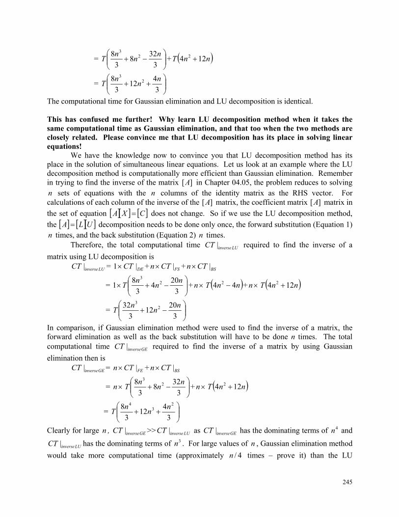
245

=

3

328

3

8 23 n

nn

T + nnT 124 2

=

3

412

3

8 23 n

nn

T

The computational time for Gaussian elimination and LU decomposition is identical. This has confused me further! Why learn LU decomposition method when it takes the same computational time as Gaussian elimination, and that too when the two methods are closely related. Please convince me that LU decomposition has its place in solving linear equations!

We have the knowledge now to convince you that LU decomposition method has its place in the solution of simultaneous linear equations. Let us look at an example where the LU decomposition method is computationally more efficient than Gaussian elimination. Remember in trying to find the inverse of the matrix ][A in Chapter 04.05, the problem reduces to solving n sets of equations with the n columns of the identity matrix as the RHS vector. For calculations of each column of the inverse of the ][A matrix, the coefficient matrix ][A matrix in

the set of equation CXA does not change. So if we use the LU decomposition method,

the ULA decomposition needs to be done only once, the forward substitution (Equation 1) n times, and the back substitution (Equation 2) n times.

Therefore, the total computational time LUinverseCT | required to find the inverse of a

matrix using LU decomposition is

LUinverseCT | = DECT |1 + FSCTn | + BSCTn |

=

3

204

3

81 2

3 nn

nT + n nnT 44 2 + n nnT 124 2

=

3

2012

3

32 23 n

nn

T

In comparison, if Gaussian elimination method were used to find the inverse of a matrix, the forward elimination as well as the back substitution will have to be done n times. The total computational time GEinverseCT | required to find the inverse of a matrix by using Gaussian

elimination then is

GEinverseCT | = FECTn | + BSCTn |

= n

3

328

3

8 23 n

nn

T + n nnT 124 2

=

3

412

3

8 23

4 nn

nT

Clearly for large n , GEinverseCT | >> LUinverseCT | as GEinverseCT | has the dominating terms of 4n and

LUinverseCT | has the dominating terms of 3n . For large values of n , Gaussian elimination method

would take more computational time (approximately 4/n times – prove it) than the LU

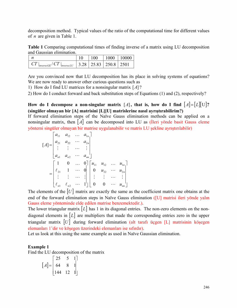
246

decomposition method. Typical values of the ratio of the computational time for different values of n are given in Table 1. Table 1 Comparing computational times of finding inverse of a matrix using LU decomposition and Gaussian elimination.

n 10 100 1000 10000

GEinverseCT | / LUinverseCT | 3.28 25.83 250.8 2501

Are you convinced now that LU decomposition has its place in solving systems of equations? We are now ready to answer other curious questions such as 1) How do I find LU matrices for a nonsingular matrix ][A ? 2) How do I conduct forward and back substitution steps of Equations (1) and (2), respectively? How do I decompose a non-singular matrix ][A , that is, how do I find U LA ? (singüler olmayan bir [A] matrisini [L][U] matrislerine nasıl ayrıştırabilirim?) If forward elimination steps of the Naïve Gauss elimination methods can be applied on a nonsingular matrix, then A can be decomposed into LU as (İleri yönde basit Gauss eleme yöntemi singüler olmayan bir matrise uygulanabilir ve matris LU şekline ayrıştırılabilir)

nnnn

n

n

aaa

aaa

aaa

A

21

22221

11211

][

nn

n

n

nn u

uu

uuu

00

0

1

01

001

222

11211

21

21

The elements of the U matrix are exactly the same as the coefficient matrix one obtains at the end of the forward elimination steps in Naïve Gauss elimination ([U] matrisi ileri yönde yalın Gauss eleme yönteminde elde edilen matrise benzemektedir.). The lower triangular matrix L has 1 in its diagonal entries. The non-zero elements on the non-

diagonal elements in L are multipliers that made the corresponding entries zero in the upper

triangular matrix U during forward elimination (alt tarafı üçgen [L] matrisinin köşegen elemanları 1’dir ve köşegen üzerindeki elemanları ise sıfırdır). Let us look at this using the same example as used in Naïve Gaussian elimination.

Example 1 Find the LU decomposition of the matrix

112144

1864

1525

A

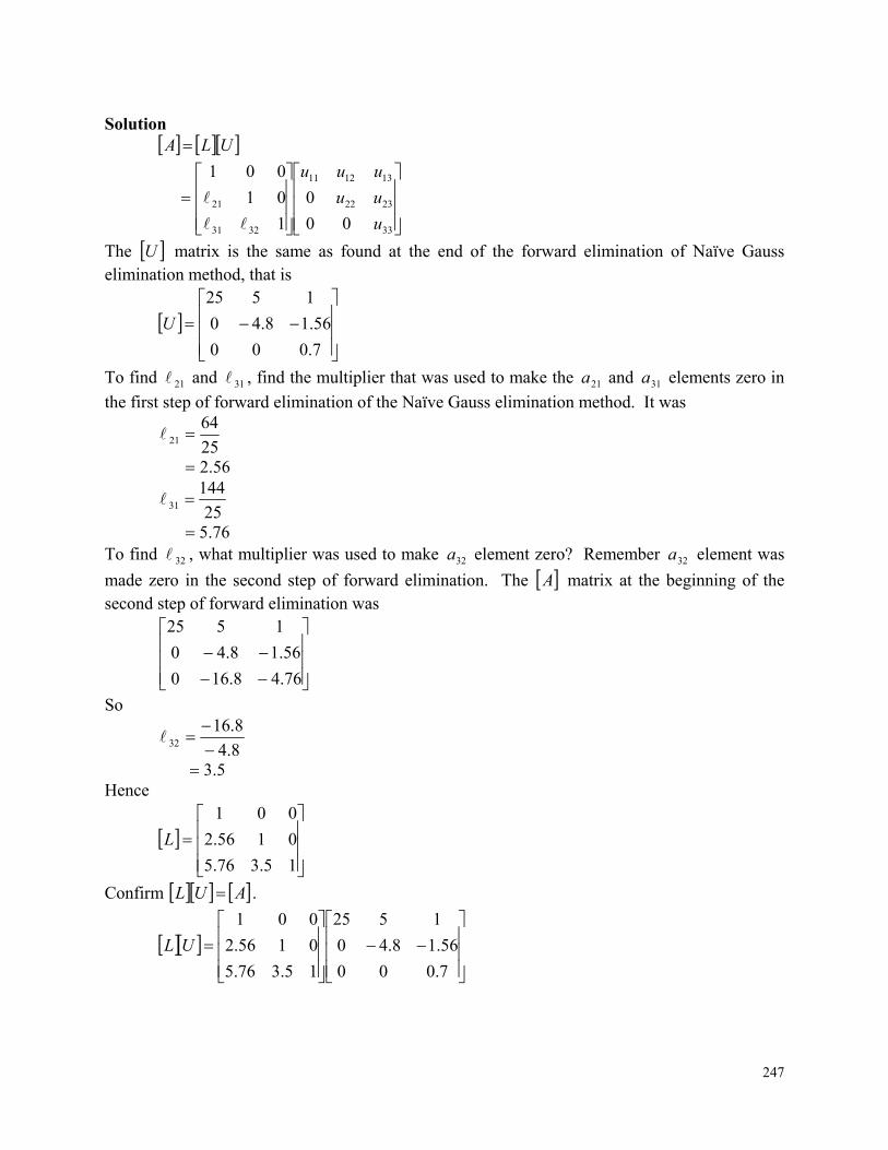
247

Solution ULA

33

2322

131211

3231

21

00

0

1

01

001

u

uu

uuu

The U matrix is the same as found at the end of the forward elimination of Naïve Gauss elimination method, that is

7.000

56.18.40

1525

U

To find 21 and 31 , find the multiplier that was used to make the 21a and 31a elements zero in

the first step of forward elimination of the Naïve Gauss elimination method. It was

25

6421

56.2

25

14431

76.5 To find 32 , what multiplier was used to make 32a element zero? Remember 32a element was

made zero in the second step of forward elimination. The A matrix at the beginning of the second step of forward elimination was

76.48.160

56.18.40

1525

So

8.4

8.1632

5.3 Hence

15.376.5

0156.2

001

L

Confirm AUL .

7.000

56.18.40

1525

15.376.5

0156.2

001

UL

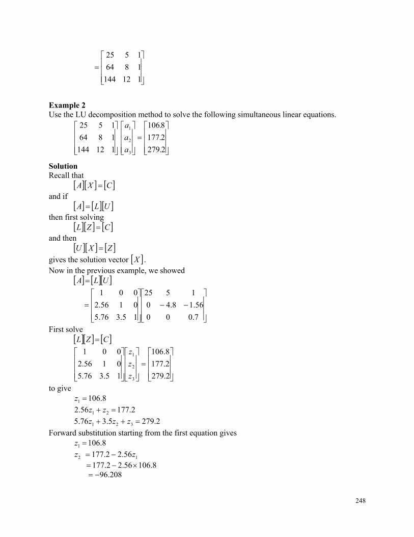
248

112144

1864

1525

Example 2 Use the LU decomposition method to solve the following simultaneous linear equations.

2279

2177

8106

112144

1864

1525

3

2

1

.

.

.

a

a

a

Solution Recall that

CXA and if

ULA then first solving

CZL and then

ZXU

gives the solution vector X . Now in the previous example, we showed

ULA

7.000

56.18.40

1525

15.376.5

0156.2

001

First solve CZL

2.279

2.177

8.106

15.376.5

0156.2

001

3

2

1

z

z

z

to give 8.1061 z

2.17756.2 21 zz

2.2795.376.5 321 zzz

Forward substitution starting from the first equation gives 106.8 1 z

12 56.22.177 z z 8.10656.22.177 208.96

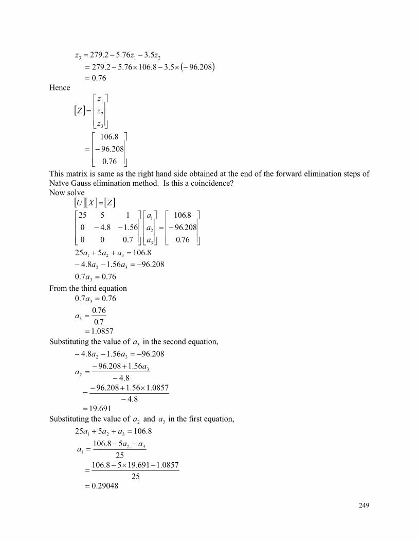
249

213 5.376.52.279 zzz

208.965.38.10676.52.279 76.0

Hence

3

2

1

z

z

z

Z

76.0

208.96

8.106

This matrix is same as the right hand side obtained at the end of the forward elimination steps of Naïve Gauss elimination method. Is this a coincidence? Now solve

ZXU

760

20896

8106

7.000

56.18.40

1525

3

2

1

.

.

.

a

a

a

8.106525 321 aaa

208.9656.18.4 32 aa

76.07.0 3 a

From the third equation 76.07.0 3 a

70

7603 .

.a

1.0857 Substituting the value of 3a in the second equation,

208.9656.18.4 32 aa

8.4

56.1208.96 32

aa

4.8

0857.11.5696.208

69119. Substituting the value of 2a and 3a in the first equation,

8.106525 321 aaa

25

58.106 32

1

aaa

25

0857.1691.1958.106

29048.0

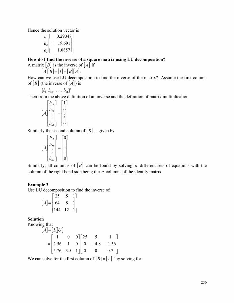
250

Hence the solution vector is

0857.1

691.19

29048.0

3

2

1

a

a

a

How do I find the inverse of a square matrix using LU decomposition? A matrix B is the inverse of A if

ABIBA . How can we use LU decomposition to find the inverse of the matrix? Assume the first column of B (the inverse of A ) is

T11211 ]......[ nbbb

Then from the above definition of an inverse and the definition of matrix multiplication

0

0

1

1

21

11

nb

b

b

A

Similarly the second column of B is given by

0

1

0

2

22

12

nb

b

b

A

Similarly, all columns of B can be found by solving n different sets of equations with the column of the right hand side being the n columns of the identity matrix.

Example 3 Use LU decomposition to find the inverse of

112144

1864

1525

A

Solution Knowing that

ULA

0.700

1.564.80

1525

15.376.5

0156.2

001

We can solve for the first column of 1][ AB by solving for

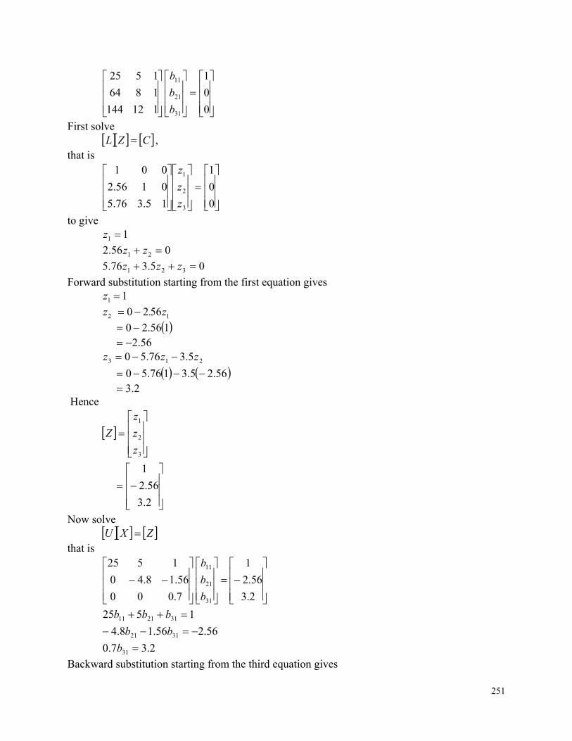
251

0

0

1

112144

1864

1525

31

21

11

b

b

b

First solve CZL ,

that is

0

0

1

15.376.5

0156.2

001

3

2

1

z

z

z

to give 11 z

056.2 21 zz

05.376.5 321 zzz

Forward substitution starting from the first equation gives 1 1 z

12 5620 z. z

156.20 56.2

213 5.376.50 zzz

56.25.3176.50 2.3

Hence

3

2

1

z

z

z

Z

2.3

56.2

1

Now solve ZXU

that is

3.2

2.56

1

7.000

56.18.40

1525

31

21

11

b

b

b

1525 312111 bbb

56.256.18.4 3121 bb

2.37.0 31 b

Backward substitution starting from the third equation gives

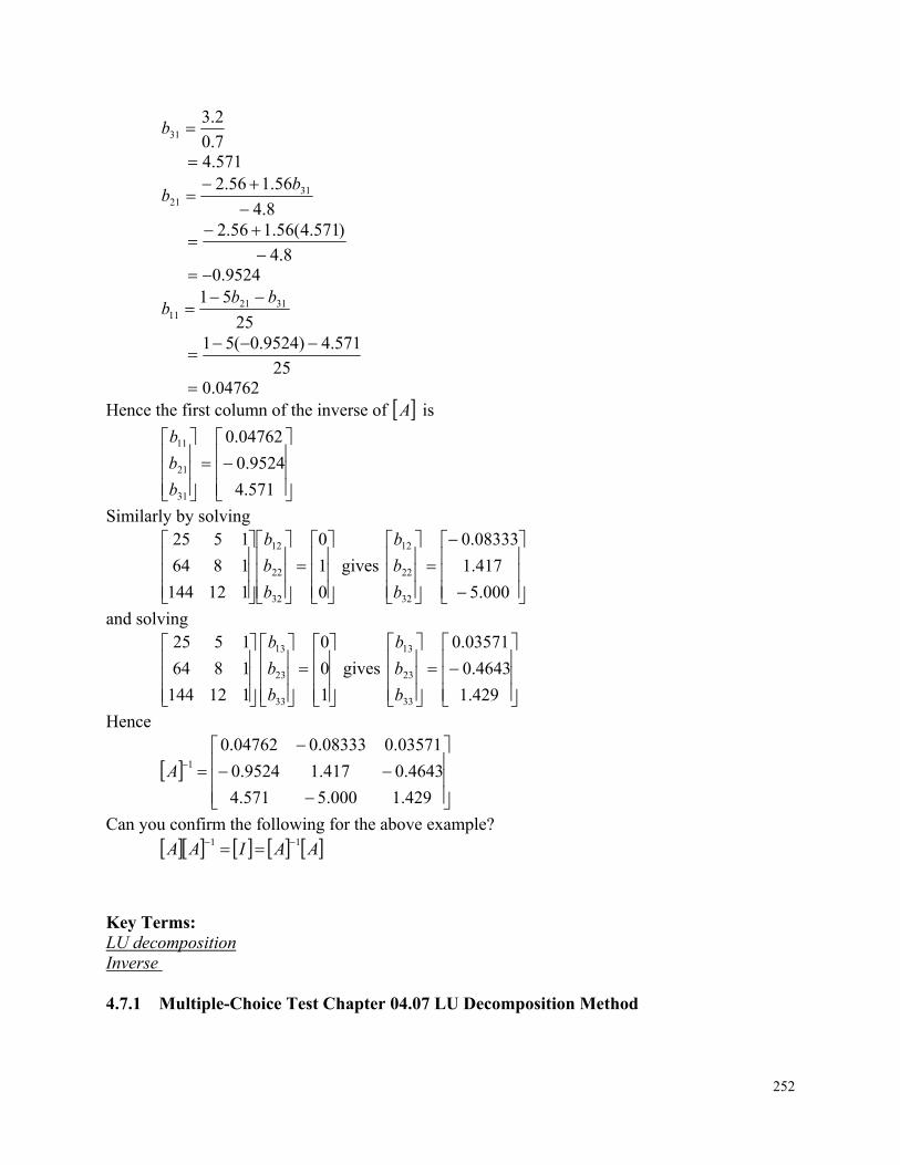
252

7.0

2.331 b

571.4

8.4

56.156.2 3121

bb

8.4

)571.4(56.156.2

9524.0

25

51 312111

bbb

25

571.4)9524.0(51

04762.0 Hence the first column of the inverse of A is

571.4

9524.0

04762.0

31

21

11

b

b

b

Similarly by solving

0

1

0

112144

1864

1525

32

22

12

b

b

b

gives

000.5

417.1

08333.0

32

22

12

b

b

b

and solving

1

0

0

112144

1864

1525

33

23

13

b

b

b

gives

429.1

4643.0

03571.0

33

23

13

b

b

b

Hence

429.1000.5571.4

4643.0417.19524.0

03571.008333.004762.01A

Can you confirm the following for the above example?

AAIAA 11

Key Terms: LU decomposition Inverse 4.7.1 Multiple-Choice Test Chapter 04.07 LU Decomposition Method

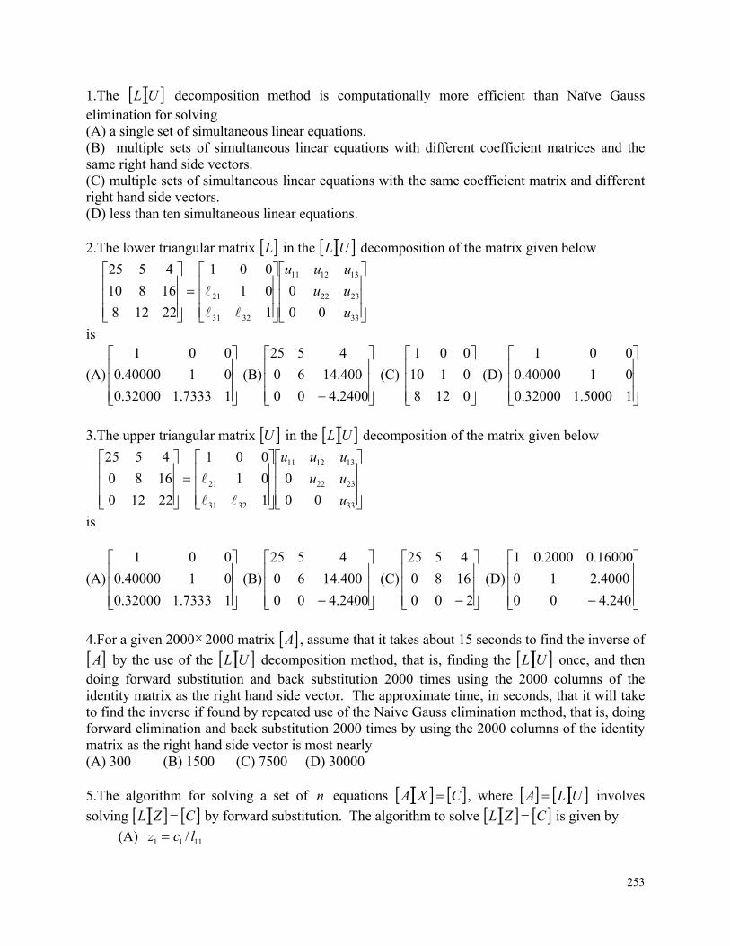
253

1.The UL decomposition method is computationally more efficient than Naïve Gauss elimination for solving (A) a single set of simultaneous linear equations. (B) multiple sets of simultaneous linear equations with different coefficient matrices and the same right hand side vectors. (C) multiple sets of simultaneous linear equations with the same coefficient matrix and different right hand side vectors. (D) less than ten simultaneous linear equations. 2.The lower triangular matrix L in the UL decomposition of the matrix given below

33

2322

131211

3231

21

00

0

1

01

001

22128

16810

4525

u

uu

uuu

is

(A)

17333.132000.0

0140000.0

001

(B)

2400.400

400.1460

4525

(C)

0128

0110

001

(D)

15000.132000.0

0140000.0

001

3.The upper triangular matrix U in the UL decomposition of the matrix given below

33

2322

131211

3231

21

00

0

1

01

001

22120

1680

4525

u

uu

uuu

is

(A)

17333.132000.0

0140000.0

001

(B)

2400.400

400.1460

4525

(C)

200

1680

4525

(D)

240.400

4000.210

16000.02000.01

4.For a given 20002000 matrix A , assume that it takes about 15 seconds to find the inverse of

A by the use of the UL decomposition method, that is, finding the UL once, and then doing forward substitution and back substitution 2000 times using the 2000 columns of the identity matrix as the right hand side vector. The approximate time, in seconds, that it will take to find the inverse if found by repeated use of the Naive Gauss elimination method, that is, doing forward elimination and back substitution 2000 times by using the 2000 columns of the identity matrix as the right hand side vector is most nearly (A) 300 (B) 1500 (C) 7500 (D) 30000 5.The algorithm for solving a set of n equations CXA , where ULA involves

solving CZL by forward substitution. The algorithm to solve CZL is given by

(A) 1111 / lcz

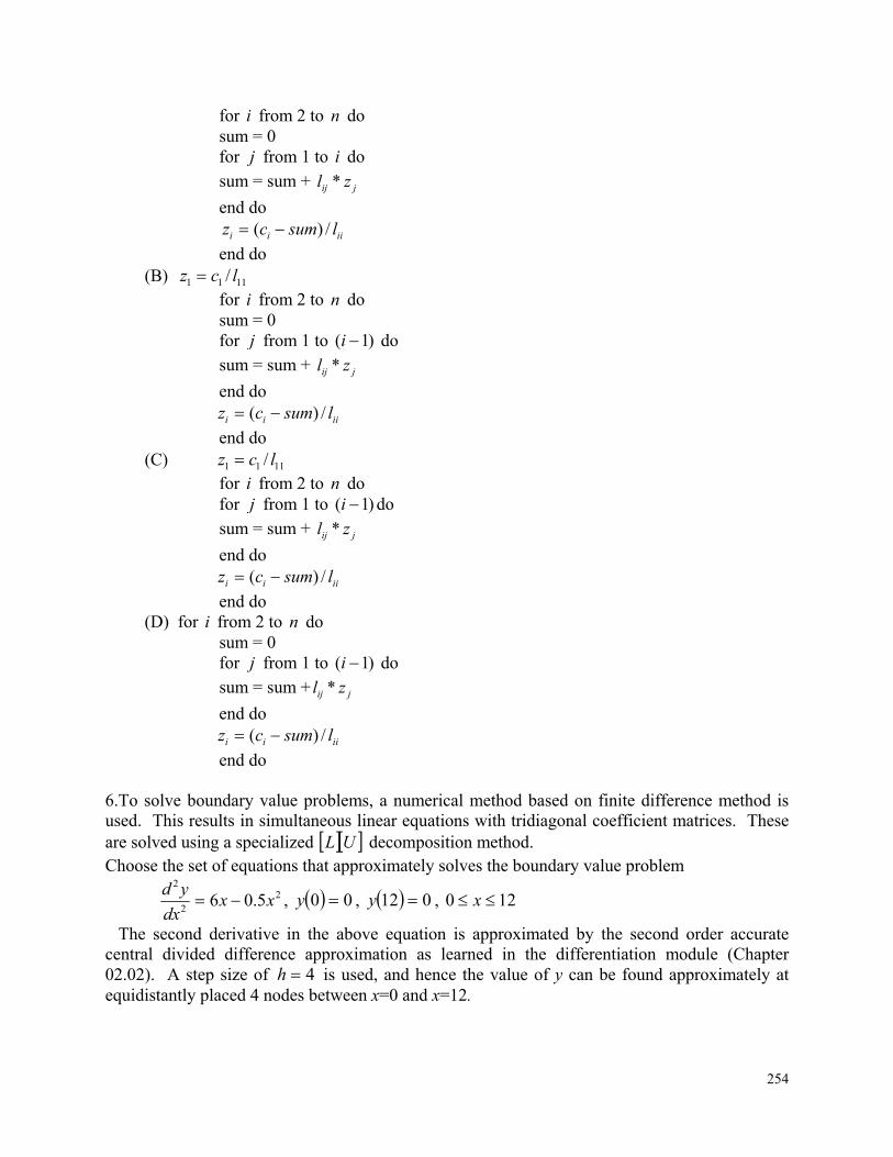
254

for i from 2 to n do sum = 0 for j from 1 to i do

sum = sum + jij zl *

end do iiii lsumcz /)(

end do (B) 1111 / lcz for i from 2 to n do sum = 0 for j from 1 to )1( i do

sum = sum + jij zl *

end do iiii lsumcz /)(

end do (C) 1111 / lcz for i from 2 to n do for j from 1 to )1( i do

sum = sum + jij zl *

end do iiii lsumcz /)(

end do (D) for i from 2 to n do sum = 0 for j from 1 to )1( i do

sum = sum + jij zl *

end do iiii lsumcz /)(

end do 6.To solve boundary value problems, a numerical method based on finite difference method is used. This results in simultaneous linear equations with tridiagonal coefficient matrices. These are solved using a specialized UL decomposition method. Choose the set of equations that approximately solves the boundary value problem

22

2

5.06 xxdx

yd , 00 y , 012 y , 120 x

The second derivative in the above equation is approximated by the second order accurate central divided difference approximation as learned in the differentiation module (Chapter 02.02). A step size of 4h is used, and hence the value of y can be found approximately at equidistantly placed 4 nodes between x=0 and x=12.

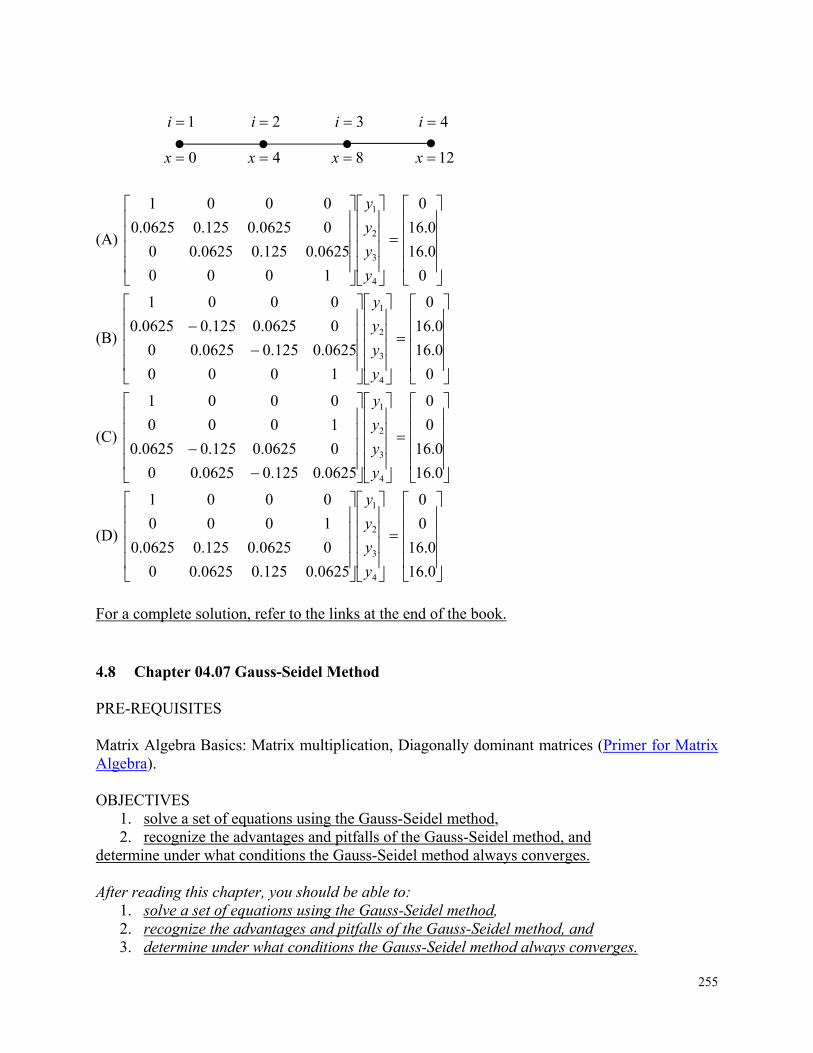
255

(A)

0

0.16

0.16

0

1000

0625.0125.00625.00

00625.0125.00625.0

0001

4

3

2

1

y

y

y

y

(B)

0

0.16

0.16

0

1000

0625.0125.00625.00

00625.0125.00625.0

0001

4

3

2

1

y

y

y

y

(C)

0.16

0.16

0

0

0625.0125.00625.00

00625.0125.00625.0

1000

0001

4

3

2

1

y

y

y

y

(D)

0.16

0.16

0

0

0625.0125.00625.00

00625.0125.00625.0

1000

0001

4

3

2

1

y

y

y

y

For a complete solution, refer to the links at the end of the book. 4.8 Chapter 04.07 Gauss-Seidel Method

PRE-REQUISITES

Matrix Algebra Basics: Matrix multiplication, Diagonally dominant matrices (Primer for Matrix Algebra).

OBJECTIVES

1. solve a set of equations using the Gauss-Seidel method, 2. recognize the advantages and pitfalls of the Gauss-Seidel method, and

determine under what conditions the Gauss-Seidel method always converges. After reading this chapter, you should be able to:

1. solve a set of equations using the Gauss-Seidel method, 2. recognize the advantages and pitfalls of the Gauss-Seidel method, and 3. determine under what conditions the Gauss-Seidel method always converges.

0x 4x 8x

1i 2i 3i 4i

12x

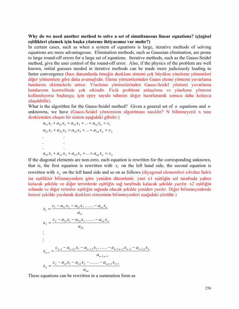
256

Why do we need another method to solve a set of simultaneous linear equations? (çizgisel eşitlikleri çözmek için başka yönteme ihtiyacımız var mıdır?) In certain cases, such as when a system of equations is large, iterative methods of solving equations are more advantageous. Elimination methods, such as Gaussian elimination, are prone to large round-off errors for a large set of equations. Iterative methods, such as the Gauss-Seidel method, give the user control of the round-off error. Also, if the physics of the problem are well known, initial guesses needed in iterative methods can be made more judiciously leading to faster convergence (bazı durumlarda örneğin denklem sistemi çok büyükse yineleme yöntemleri diğer yöntemlere göre daha avantajlıdır. Eleme yöntemlerinden Gauss eleme yöntemi yuvarlama hatalarını eklemelerle artırır. Yineleme yöntemlerinden Gauss-Seidel yöntemi yuvarlama hatalarının kontrolünde çok etkindir. Fizik problemi anlaşılırsa ve yineleme yöntemi kullanılıyorsa başlangıç için epey sayıda tahmini değer hazırlanarak sonuca daha kolayca ulaşılabilir). What is the algorithm for the Gauss-Seidel method? Given a general set of n equations and n unknowns, we have (Gauss-Seidel yönteminin algoritması nasıldır? N bilinmeyenli n tane denklemden oluşan bir sistem aşağıdaki gibidir:)

11313212111 ... cxaxaxaxa nn

22323222121 ... cxaxaxaxa nn

. .

. .

. .

nnnnnnn cxaxaxaxa ...332211

If the diagonal elements are non-zero, each equation is rewritten for the corresponding unknown, that is, the first equation is rewritten with 1x on the left hand side, the second equation is

rewritten with 2x on the left hand side and so on as follows (diyagonal elementleri sıfırdan farklı ise eşitlikler bilinmeyenlere göre yeniden düzenlenir. yani x1 eşitliğin sol tarafında yalnız kalacak şekilde ve diğer terimlerde eşitliğin sağ tarafında kalacak şekilde yazılır. x2 eşitliğin solunda ve diğer terimler eşitliğin sağında olacak şekilde yeniden yazılır. Diğer bilinmeyenlerde benzer şekilde yazılarak denklem sisteminin bilinmeyenleri aşağıdaki çözülür.)

nn

nnnnnnn

nn

nnnnnnnnnn

nn

nn

a

xaxaxacx

a

xaxaxaxacx

a

xaxaxacx

a

xaxaxacx

11,2211

1,1

,122,122,111,111

22

232312122

11

131321211

These equations can be rewritten in a summation form as

257

11

11

11

1 a

xac

x

n

jj

jj

22

21

22

2 a

xac

x

j

n

jj

j

. .

.

1,1

11

,11

1

nn

n

njj

jjnn

n a

xac

x

nn

n

njj

jnjn

n a

xac

x

1

Hence for any row i ,

.,,2,1,1

nia

xac

xii

n

ijj

jiji

i

Now to find ix ’s, one assumes an initial guess for the ix ’s and then uses the rewritten equations

to calculate the new estimates. Remember, one always uses the most recent estimates to calculate the next estimates, ix . At the end of each iteration, one calculates the absolute relative

approximate error for each ix as (artık xi’leri belirleyebilmek için xi’ler için başlangıç tahmin

değerlerine ihtiyaç vardır ve bu değerlere göre yeni hesaplamalar yapılır. Her yineleme sonunda xi’ler için mutlak bağıl yaklaşık hata hesabı yapılır:)

100new

oldnew

i

ii

iax

xx

where newix is the recently obtained value of ix , and old

ix is the previous value of ix .

When the absolute relative approximate error for each xi is less than the pre-specified tolerance, the iterations are stopped.

Example 1 The upward velocity of a rocket is given at three different times in the following table

Table 1 Velocity vs. time data.

Time, t (s) Velocity, v (m/s)

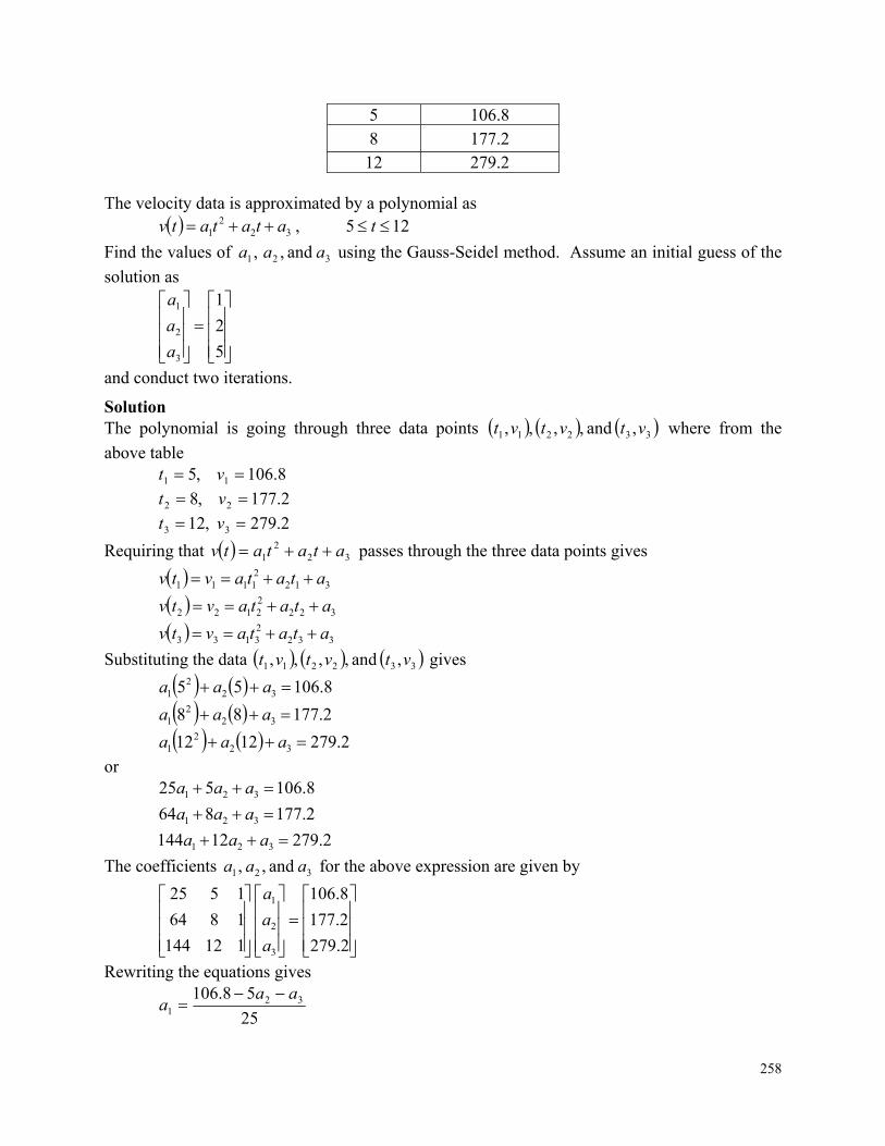
258

5 106.8 8 177.2 12 279.2

The velocity data is approximated by a polynomial as

125 , 322

1 tatatatv

Find the values of 321 and ,, aaa using the Gauss-Seidel method. Assume an initial guess of the

solution as

5

2

1

3

2

1

a

a

a

and conduct two iterations.

Solution The polynomial is going through three data points 332211 , and ,, ,, vtvtvt where from the

above table 8.106 ,5 11 vt

2.177 ,8 22 vt

2.279 ,12 33 vt

Requiring that 322

1 atatatv passes through the three data points gives

31221111 atatavtv

32222122 atatavtv

33223133 atatavtv

Substituting the data 332211 , and ,, ,, vtvtvt gives

8.10655 322

1 aaa

2.17788 322

1 aaa

2.2791212 322

1 aaa

or 8.106525 321 aaa

2.177864 321 aaa

2.27912144 321 aaa

The coefficients 321 and , , aaa for the above expression are given by

2.279

2.177

8.106

112144

1864

1525

3

2

1

a

a

a

Rewriting the equations gives

25

58.106 321

aaa

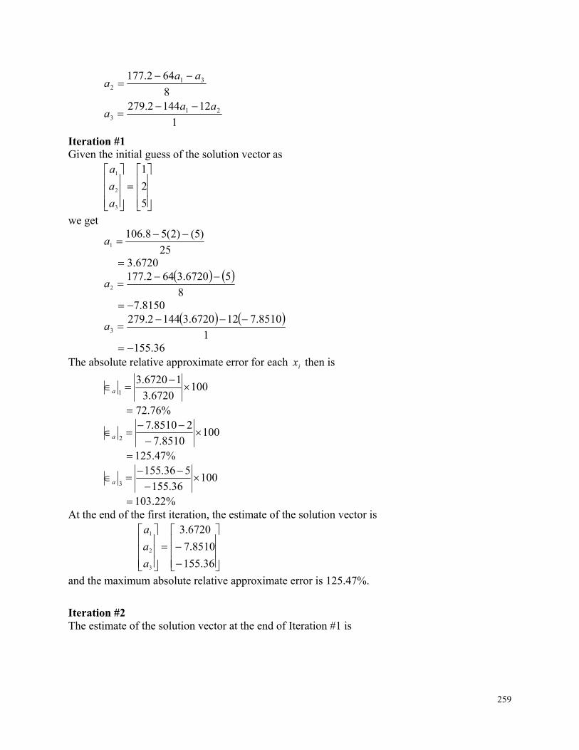
259

8

642.177 312

aaa

1

121442.279 213

aaa

Iteration #1 Given the initial guess of the solution vector as

5

2

1

3

2

1

a

a

a

we get

25

)5()2(58.1061

a

6720.3 8

56720.3642.1772

a

8150.7

1

8510.7126720.31442.2793

a

36.155 The absolute relative approximate error for each ix then is

1006720.3

16720.31

a

%76.72

1008510.7

28510.72

a

%47.125

10036.155

536.1553

a

%22.103 At the end of the first iteration, the estimate of the solution vector is

36.155

8510.7

6720.3

3

2

1

a

a

a

and the maximum absolute relative approximate error is 125.47%.

Iteration #2 The estimate of the solution vector at the end of Iteration #1 is

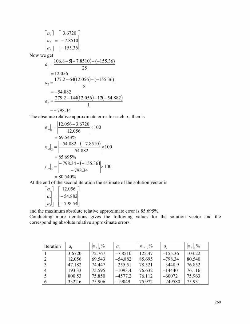
260

36.155

8510.7

6720.3

3

2

1

a

a

a

Now we get

25

)36.155(8510.758.1061

a

056.12

8

)36.155(056.12642.1772

a

882.54

1

882.5412056.121442.2793

a

= 34.798 The absolute relative approximate error for each ix then is

100056.12

6720.3056.121

a

%543.69

100882.54

8510.7882.542

a

%695.85

10034.798

36.15534.7983

a

%540.80 At the end of the second iteration the estimate of the solution vector is

54.798

882.54

056.12

3

2

1

a

a

a

and the maximum absolute relative approximate error is 85.695%. Conducting more iterations gives the following values for the solution vector and the corresponding absolute relative approximate errors.

Iteration 1a %1a 2a %

2a 3a %3a

1 2 3 4 5 6

3.6720 12.056 47.182 193.33 800.53 3322.6

72.767 69.543 74.447 75.595 75.850 75.906

–7.8510 –54.882 –255.51 –1093.4 –4577.2 –19049

125.47 85.695 78.521 76.632 76.112 75.972

–155.36 –798.34 –3448.9 –14440 –60072 –249580

103.22 80.540 76.852 76.116 75.963 75.931

261

As seen in the above table, the solution estimates are not converging to the true solution of 29048.01 a

690.192 a

0857.13 a

The above system of equations does not seem to converge. Why? (yukarıdaki denklem sistemi bir sonuca yakınsamadı. Neden?) Well, a pitfall of most iterative methods is that they may or may not converge. However, the solution to a certain classes of systems of simultaneous equations does always converge using the Gauss-Seidel method. This class of system of equations is where the coefficient matrix ][A in ][]][[ CXA is diagonally dominant, that is (yineleme yöntemlerinin birçoğunda olduğu gibi bir tuzaktan dolayı bir sonuca ulaşmayabilir. Bununla birlikte belli sınıflardaki eşitlikler sistemlerinin Gauss-Seidel öteleme yöntemi ile bir sonuca yakınsanır/yaklaşılır. [A][X]=[C] şeklinde bu eşitlikler sistemlerinin [A] katsayılar matrisinin diyagonalleri diğer terimlere göre baskındır/dominanttır:)

n

ijj

ijii aa1

for all i

n

ijj

ijii aa1

for at least one i

If a system of equations has a coefficient matrix that is not diagonally dominant, it may or may not converge. Fortunately, many physical systems that result in simultaneous linear equations have a diagonally dominant coefficient matrix, which then assures convergence for iterative methods such as the Gauss-Seidel method of solving simultaneous linear equations (diyagonal elemanları diğer elemanlarına göre baskın olmayan katsayılar matrisinin kullanılmasıyla yapılan denklem sistemlerinin çözümleri bizi bir sonuca ulaştırabilir veya ulaştırmayabilir. Neyse ki birçok fiziksel sistemin katsayılar matrisi dominanttır ve Gauss-Seidel yöntemiyle çizgisel denklem sistemlerinin aynı anda çözümünde bir sonuca ulaşılır.).

Example 2 Find the solution to the following system of equations using the Gauss-Seidel method.

15312 321 xx x

2835 321 x x x

761373 321 x x x

Use

1

0

1

3

2

1

x

x

x

as the initial guess and conduct two iterations.

Solution The coefficient matrix

262

1373

351

5312

A

is diagonally dominant as 8531212 131211 aaa

43155 232122 aaa

10731313 323133 aaa

and the inequality is strictly greater than for at least one row. Hence, the solution should converge using the Gauss-Seidel method. Rewriting the equations, we get

12

531 321

xxx

5

328 312

xxx

13

7376 213

xxx

Assuming an initial guess of

1

0

1

3

2

1

x

x

x

Iteration #1 12

150311

x

50000.0

5

1350000.0282

x

9000.4

13

9000.4750000.03763

x

0923.3 The absolute relative approximate error at the end of the first iteration is

10050000.0

150000.01

a

%00.100

1009000.4

09000.42

a

%00.100

1000923.3

10923.33

a

263

%662.67 The maximum absolute relative approximate error is 100.00%

Iteration #2

12

0923.359000.4311

x

14679.0

5

0923.3314679.0282

x

7153.3

13

7153.3714679.03763

x

8118.3 At the end of second iteration, the absolute relative approximate error is

10014679.0

50000.014679.01

a

%61.240

1007153.3

9000.47153.32

a

%889.31

1008118.3

0923.38118.33

a

%874.18 The maximum absolute relative approximate error is 240.61%. This is greater than the value of 100.00% we obtained in the first iteration. Is the solution diverging? No, as you conduct more iterations, the solution converges as follows.

Iteration 1x %1a 2x %

2a 3x %3a

1 2 3 4 5 6

0.50000 0.14679 0.74275 0.94675 0.99177 0.99919

100.00 240.61 80.236 21.546 4.5391 0.74307

4.9000 3.7153 3.1644 3.0281 3.0034 3.0001

100.00 31.889 17.408 4.4996 0.82499 0.10856

3.0923 3.8118 3.9708 3.9971 4.0001 4.0001

67.662 18.874 4.0064 0.65772 0.074383 0.00101

This is close to the exact solution vector of

4

3

1

3

2

1

x

x

x

Example 3 Given the system of equations

264

761373 321 x x x

2835 321 x x x

15312 321 x - x x

find the solution using the Gauss-Seidel method. Use

1

0

1

3

2

1

x

x

x

as the initial guess.

Solution Rewriting the equations, we get

3

13776 321

xxx

5

328 312

xxx

5

3121 213

xxx

Assuming an initial guess of

1

0

1

3

2

1

x

x

x

the next six iterative values are given in the table below.

Iteration 1x %1a 2x %

2a 3x %3a

1 2 3 4 5 6

21.000 –196.15 1995.0 –20149 2.0364105 –2.0579106

95.238 110.71 109.83 109.90 109.89 109.89

0.80000 14.421 –116.02 1204.6 –12140 1.2272105

100.00 94.453 112.43 109.63 109.92 109.89

50.680 –462.30 4718.1 –47636 4.8144105 –4.8653106

98.027 110.96 109.80 109.90 109.89 109.89

You can see that this solution is not converging and the coefficient matrix is not diagonally dominant. The coefficient matrix

5312

351

1373

A

is not diagonally dominant as 2013733 131211 aaa

Hence, the Gauss-Seidel method may or may not converge.

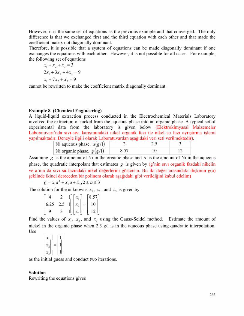
265

However, it is the same set of equations as the previous example and that converged. The only difference is that we exchanged first and the third equation with each other and that made the coefficient matrix not diagonally dominant. Therefore, it is possible that a system of equations can be made diagonally dominant if one exchanges the equations with each other. However, it is not possible for all cases. For example, the following set of equations

3321 xxx

9432 321 xxx

97 321 xxx

cannot be rewritten to make the coefficient matrix diagonally dominant.

Example 8 (Chemical Engineering) A liquid-liquid extraction process conducted in the Electrochemical Materials Laboratory involved the extraction of nickel from the aqueous phase into an organic phase. A typical set of experimental data from the laboratory is given below (Elektrokimyasal Malzemeler Laboratuvarı’nda sıvı-sıvı karışımındaki nikel organik fazı ile nikel su fazı ayrıştırma işlemi yapılmaktadır. Deneyle ilgili olarak Laboratuvardan aşağıdaki veri seti verilmektedir).

Ni aqueous phase, lga 2 2.5 3

Ni organic phase, lgg 8.57 10 12

Assuming g is the amount of Ni in the organic phase and a is the amount of Ni in the aqueous phase, the quadratic interpolant that estimates g is given by (g’nin sıvı organik fazdaki nikelin ve a’nın da sıvı su fazındaki nikel değerlerini göstersin. Bu iki değer arasındaki ilişkinin g(a) şeklinde ikinci dereceden bir polinom olarak aşağıdaki gibi verildiğini kabul edelim)

32,322

1 axaxaxg

The solution for the unknowns 1x , 2x , and 3x is given by

12

10

57.8

139

15.225.6

124

3

2

1

x

x

x

Find the values of 1x , 2x , and 3x using the Gauss-Seidel method. Estimate the amount of

nickel in the organic phase when 2.3 g/l is in the aqueous phase using quadratic interpolation. Use

1

1

1

3

2

1

x

x

x

as the initial guess and conduct two iterations.

Solution Rewriting the equations gives

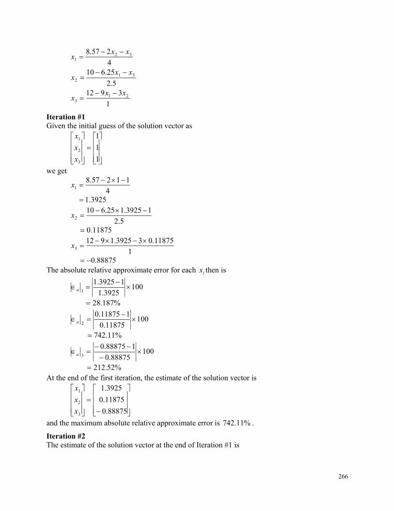
266

4

257.8 321

xxx

5.2

25.610 312

xxx

1

3912 213

xxx

Iteration #1 Given the initial guess of the solution vector as

1

1

1

3

2

1

x

x

x

we get

4

11257.81

x

3925.1

5.2

13925.125.6102

x

11875.0

1

11875.033925.19123

x

88875.0 The absolute relative approximate error for each ix then is

1003925.1

13925.11

a

%187.28

10011875.0

111875.02

a

%11.742

10088875.0

188875.03

a

%52.212 At the end of the first iteration, the estimate of the solution vector is

88875.0

11875.0

3925.1

3

2

1

x

x

x

and the maximum absolute relative approximate error is %11.742 .

Iteration #2 The estimate of the solution vector at the end of Iteration #1 is

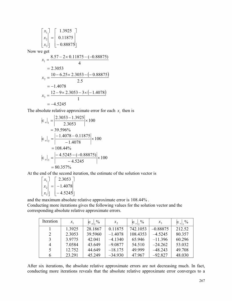
267

88875.0

11875.0

3925.1

3

2

1

x

x

x

Now we get

4

)88875.0(11875.0257.81

x

3053.2

5.2

88875.03053.225.6102

x

4078.1

1

4078.133053.29123

x

5245.4

The absolute relative approximate error for each ix then is

1003053.2

3925.13053.21

a

%596.39

1004078.1

11875.04078.12

a

%44.108

1005245.4

)88875.0(5245.43

a

%357.80 At the end of the second iteration, the estimate of the solution vector is

5245.4

4078.1

3053.2

3

2

1

x

x

x

and the maximum absolute relative approximate error is %44.108 . Conducting more iterations gives the following values for the solution vector and the corresponding absolute relative approximate errors.

Iteration 1x %

1a 2x %2a 3x %

3a 1 2 3 4 5 6

1.3925 2.3053 3.9775 7.0584 12.752 23.291

28.1867 39.5960 42.041 43.649 44.649 45.249

0.11875 –1.4078 –4.1340 –9.0877 –18.175 –34.930

742.1053 108.4353 65.946 54.510 49.999 47.967

–0.88875 –4.5245 –11.396 –24.262 –48.243 –92.827

212.52 80.357 60.296 53.032 49.708 48.030

After six iterations, the absolute relative approximate errors are not decreasing much. In fact, conducting more iterations reveals that the absolute relative approximate error converges to a

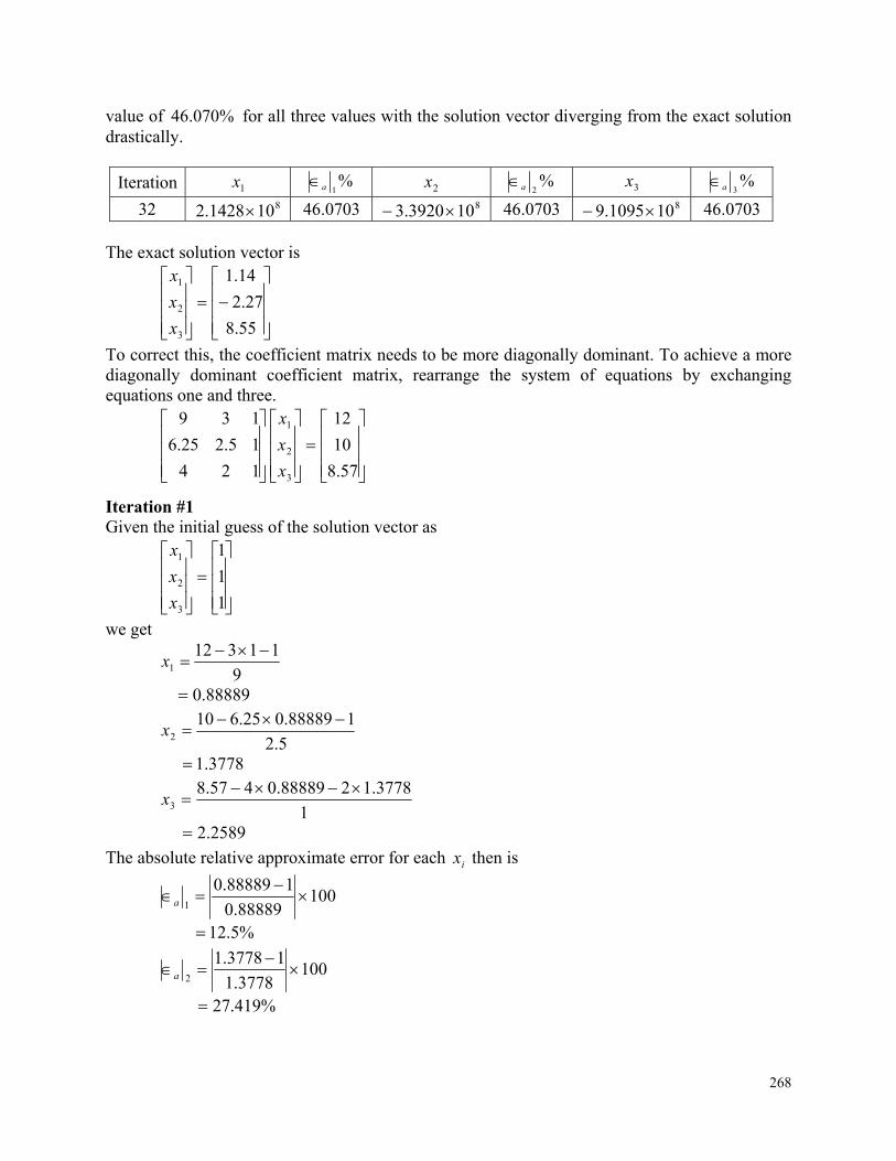
268

value of %070.46 for all three values with the solution vector diverging from the exact solution drastically.

Iteration 1x %1a 2x %

2a 3x %3a

32 8101428.2 0703.46 8103920.3 0703.46 8101095.9 0703.46 The exact solution vector is

55.8

27.2

14.1

3

2

1

x

x

x

To correct this, the coefficient matrix needs to be more diagonally dominant. To achieve a more diagonally dominant coefficient matrix, rearrange the system of equations by exchanging equations one and three.

57.8

10

12

124

15.225.6

139

3

2

1

x

x

x

Iteration #1 Given the initial guess of the solution vector as

1

1

1

3

2

1

x

x

x

we get

9

113121

x

88889.0

5.2

188889.025.6102

x

3778.1

1

3778.1288889.0457.83

x

2589.2 The absolute relative approximate error for each ix then is

10088889.0

188889.01

a

%5.12

1003778.1

13778.12

a

%419.27

269

1002589.2

12589.23

a

%730.55 At the end of the first iteration, the estimate of the solution vector is

2589.2

3778.1

88889.0

3

2

1

x

x

x

and the maximum absolute relative approximate error is %730.55 .

Iteration #2 The estimate of the solution vector at the end of Iteration #1 is

2589.2

3778.1

88889.0

3

2

1

x

x

x

Now we get

9

2589.213778.13121

x

62309.0

5.2

2589.2162309.025.6102

x

5387.1

1

5387.1262309.0457.83

x

0002.3 The absolute relative approximate error for each ix then is

10062309.0

88889.062309.01

a

%659.42

1005387.1

3778.15387.12

a

%460.10

1000002.3

2589.20002.33

a

%709.24 At the end of the second iteration, the estimate of the solution is

0002.3

5387.1

62309.0

3

2

1

x

x

x

and the maximum absolute relative approximate error is %659.42 .

270

Conducting more iterations gives the following values for the solution vector and the corresponding absolute relative approximate errors.

Iteration 1x %1a 2x %

2a 3x %3a

1 2 3 4 5 6

0.88889 0.62309 0.48707 0.42178 0.39494 0.38890

12.5 42.659 27.926 15.479 6.7960 1.5521

1.3778 1.5387 1.5822 1.5627 1.5096 1.4393

27.419 10.456 2.7506 1.2537 3.5131 4.8828

2.2589 3.0002 3.4572 3.7576 3.9710 4.1357

55.730 24.709 13.220 7.9928 5.3747 3.9826

After six iterations, the absolute relative approximate errors seem to be decreasing. Conducting more iterations allows the absolute relative approximate error decrease to an acceptable level.

Iteration 1x %1a 2x %

2a 3x %3a

199 200

1.1335 1.1337

0.014412 0.014056

–2.2389 –2.2397

0.034871 0.034005

8.5139 8.5148

0.010666 0.010403

This is close to the exact solution vector of

55.8

27.2

14.1

3

2

1

x

x

x

The polynomial that passes through the three data points is then

322

1 xaxaxag

5148.82397.21337.1 2 aa where g is the amount of nickel in the organic phase and a is the amount of nickel in the aqueous phase. When l3.2 g is in the aqueous phase, using quadratic interpolation, the estimated amount of nickel in the organic phase is

5148.83.22397.23.21337.13.2 2 g

lg3608.9

Example 9 (Civil Engineering) To find the maximum stresses in a compound cylinder, the following four simultaneous linear equations need to be solved.

0

007.0

0

10887.7

106057.3102857.400

15384.05.615384.05.6

104619.5102857.4104619.5102857.4

00102307.9102857.4 3

4

3

2

1

57

5757

57

c

c

c

c

271

In the compound cylinder, the inner cylinder has an internal radius of "5a , and an outer radius "5.6c , while the outer cylinder has an internal radius of "5.6c and an outer radius of

"8b . Given 61030E psi, 3.0 , and that the hoop stress in the outer cylinder is given by

2432

11

1 rcc

E

,

find the stress on the inside radius of the outer cylinder. Find the values of 1c , 2c , 3c and 4c using the Gauss-Seidel Method. Use

03.0

0002.0

001.0

005.0

4

3

2

1

c

c

c

c

as the initial guess and conduct two iterations.

Solution Rewriting the equations gives

7432

53

1 1028574

001023079108877

.

ccc..c

54

53

71

7

2 1046195

1046195102857410285740

.

c.c.c.c

56

153840153840560070 4213 .

c.c.c..c

5

37

214 1060573

1028574000

.

c.ccc

Iteration #1 Given the initial guess of the solution vector as

03.0

0002.0

001.0

005.0

4

3

2

1

c

c

c

c

we get

7

53

1 1028574

00101023079108877

.

...c

4106249.1

5

5747

2 1046195

0301046195000201028574106249110285740

.

......c

3105569.1

56

03015384010556911538401062491560070 34

3 .

.......c

4104125.2

272

5

47

4 1060573

104125210285740

.

..c

2108675.2 The absolute relative approximate error for each ic then is

100106249.1

005.0106249.14

4

1

a

%1.2977

100105569.1

001.0105569.13

3

2

a

%770.35

100104125.2

002.0104125.24

4

3

a

%098.17

100108675.2

03.0108675.22

2

4

a

%6223.4 At the end of the first iteration, the estimate of the solution vector is

2

4

3

4

4

3

2

1

108675.2

104125.2

105569.1

106249.1

c

c

c

c

and the maximum absolute relative approximate error is %1.2977 .

Iteration #2 The estimate of the solution vector at the end of Iteration #1 is

2

4

3

4

4

3

2

1

108675.2

104125.2

105569.1

106249.1

c

c

c

c

Now we get

7

353

1 1028574

10556911023079108877

.

...c

4105050.1

5

25

4747

2 1046195

10867521046195

10412521028574105050110285740

.

..

....

c

3100639.2

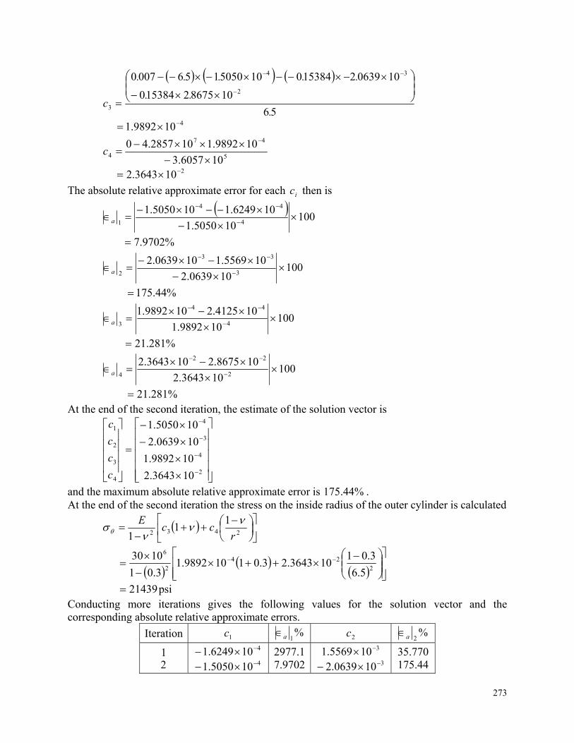
273

56

1086752153840

100639215384010505015600702

34

3 .

..

.....

c

4109892.1

5

47

4 106057.3

109892.1102857.40

c

2103643.2

The absolute relative approximate error for each ic then is

100105050.1

106249.1105050.14

44

1

a

%9702.7

100100639.2

105569.1100639.23

33

2

a

%44.175

100109892.1

104125.2109892.14

44

3

a

%281.21

100103643.2

108675.2103643.22

22

4

a

%281.21 At the end of the second iteration, the estimate of the solution vector is

2

4

3

4

4

3

2

1

103643.2

109892.1

100639.2

105050.1

c

c

c

c

and the maximum absolute relative approximate error is %44.175 . At the end of the second iteration the stress on the inside radius of the outer cylinder is calculated

2432

11

1 rcc

E

2

242

6

5.6

3.01103643.23.01109892.1

3.01

1030

psi21439 Conducting more iterations gives the following values for the solution vector and the corresponding absolute relative approximate errors.

Iteration 1c %1a 2c %

2a

1 2

4106249.1 4105050.1

2977.1 7.9702

3105569.1 3100639.2

35.770 175.44

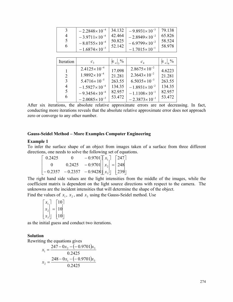
274

3 4 5 6

4102848.2 4109711.3 4100755.8 3106874.1

34.132 42.464 50.825 52.142

3108931.9 2108949.2 2109799.6 1107015.1

79.138 65.826 58.524 58.978

Iteration 3c %3a 4c %

4a

1 2 3 4 5 6

4104125.2 4109892.1 5104716.5

4105927.1 4103454.9 3100085.2

17.098 21.281 263.55 134.35 82.957 53.472

2108675.2 2103643.2 3105035.6 2108931.1 1101108.1 1103873.2

4.6223 21.281 263.55 134.35 82.957 53.472

After six iterations, the absolute relative approximate errors are not decreasing. In fact, conducting more iterations reveals that the absolute relative approximate error does not approach zero or converge to any other number.

Gauss-Seidel Method – More Examples Computer Engineering

Example 1 To infer the surface shape of an object from images taken of a surface from three different directions, one needs to solve the following set of equations.

239

248

247

9428.02357.02357.0

9701.02425.00

9701.002425.0

3

2

1

x

x

x

The right hand side values are the light intensities from the middle of the images, while the coefficient matrix is dependent on the light source directions with respect to the camera. The unknowns are the incident intensities that will determine the shape of the object. Find the values of 1x , 2x , and 3x using the Gauss-Seidel method. Use

10

10

10

3

2

1

x

x

x

as the initial guess and conduct two iterations.

Solution Rewriting the equations gives

2425.0

9701.00247 321

xxx

2425.0

9701.00248 312

xxx

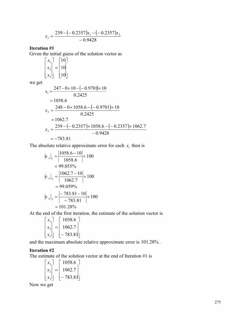
275

9428.0

2357.02357.0239 213

xxx

Iteration #1 Given the initial guess of the solution vector as

10

10

10

3

2

1

x

x

x

we get

0.2425

100.97011002471

x

6.1058

2425.0

109701.06.105802482

x

7.1062

9428.0

7.10622357.06.10582357.02393

x

81.783

The absolute relative approximate error for each ix then is

1006.1058

106.10581

a

%055.99

1007.1062

107.10622

a

%059.99

10081.783

1081.7833

a

%28.101 At the end of the first iteration, the estimate of the solution vector is

81.783

7.1062

6.1058

3

2

1

x

x

x

and the maximum absolute relative approximate error is %28.101 .

Iteration #2 The estimate of the solution vector at the end of Iteration #1 is

81.783

7.1062

6.1058

3

2

1

x

x

x

Now we get

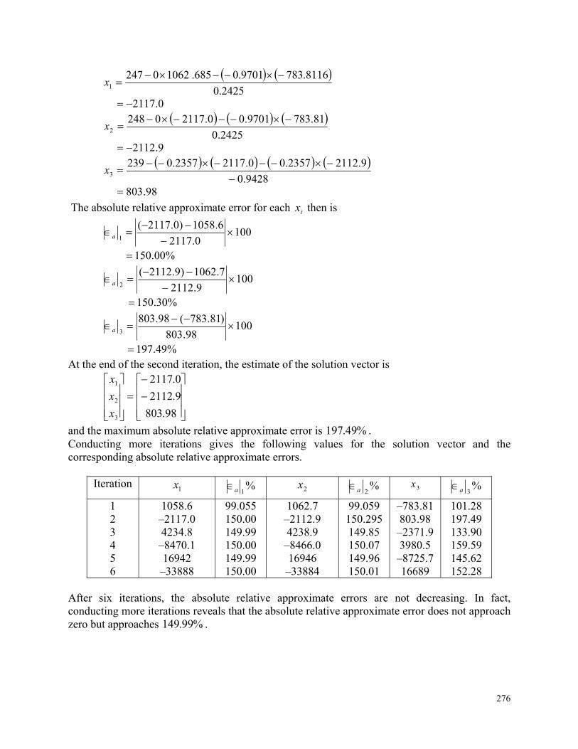
276

2425.0

8116.7839701.0685.106202471

x

0.2117

2425.0

81.7839701.00.211702482

x

9.2112

9428.0

9.21122357.00.21172357.02393

x

98.803

The absolute relative approximate error for each ix then is

1000.2117

6.1058)0.2117(1

a

%00.150

1009.2112

7.1062)9.2112(2

a

%30.150

10098.803

)81.783(98.8033

a

%49.197 At the end of the second iteration, the estimate of the solution vector is

98.803

9.2112

0.2117

3

2

1

x

x

x

and the maximum absolute relative approximate error is %49.197 . Conducting more iterations gives the following values for the solution vector and the corresponding absolute relative approximate errors.

Iteration 1x %

1a 2x %2a 3x %

3a

1 2 3 4 5 6

1058.6 –2117.0 4234.8 –8470.1 16942 –33888

99.055 150.00 149.99 150.00 149.99 150.00

1062.7 –2112.9 4238.9 –8466.0 16946 –33884

99.059 150.295 149.85 150.07 149.96 150.01

–783.81 803.98 –2371.9 3980.5 –8725.7 16689

101.28 197.49 133.90 159.59 145.62 152.28

After six iterations, the absolute relative approximate errors are not decreasing. In fact, conducting more iterations reveals that the absolute relative approximate error does not approach zero but approaches %99.149 .

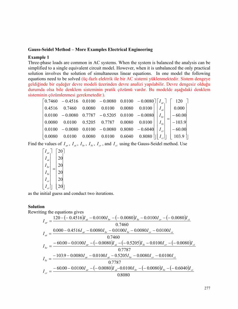
277

Gauss-Seidel Method – More Examples Electrical Engineering

Example 1 Three-phase loads are common in AC systems. When the system is balanced the analysis can be simplified to a single equivalent circuit model. However, when it is unbalanced the only practical solution involves the solution of simultaneous linear equations. In one model the following equations need to be solved (üç-fazlı elektrik ile bir AC sistemi yüklenmektedir. Sistem dengeye geldiğinde bir eşdeğer devre modeli üzerinden devre analizi yapılabilir. Devre dengesiz olduğu durumda olsa bile denklem sisteminin pratik çözümü vardır. Bu modelde aşağıdaki denklem sisteminin çözümlenmesi gerekmetedir:).

9.103

00.60

9.103

00.60

000.0

120

8080.06040.00100.00080.00100.00080.0

6040.08080.00080.00100.00080.00100.0

0100.00080.07787.05205.00100.00080.0

0080.00100.05205.07787.00080.00100.0

0100.00080.00100.00080.07460.04516.0

0080.00100.00080.00100.04516.07460.0

ci

cr

bi

br

ai

ar

I

I

I

I

I

I

Find the values of arI , aiI , brI , biI , crI , and ciI using the Gauss-Seidel method. Use

20

20

20

20

20

20

ci

cr

bi

br

ai

ar

I

I

I

I

I

I

as the initial guess and conduct two iterations.

Solution Rewriting the equations gives

7460.0

0080.00100.00080.00100.04516.0120 cicrbibraiar

IIIIII

74600

01000008000100000800451600000

.

I.I.I.I.I..I cicrbibrar

ai

77870

00800010005205000800010000060

.

I.I.I.I.I..I cicrbiaiar

br

77870

01000008005205001000008009103

.

I.I.I.I.I..I cicrbraiar

bi

80800

60400008000100000800010000060

.

I.I.I.I.I..I cibibraiar

cr

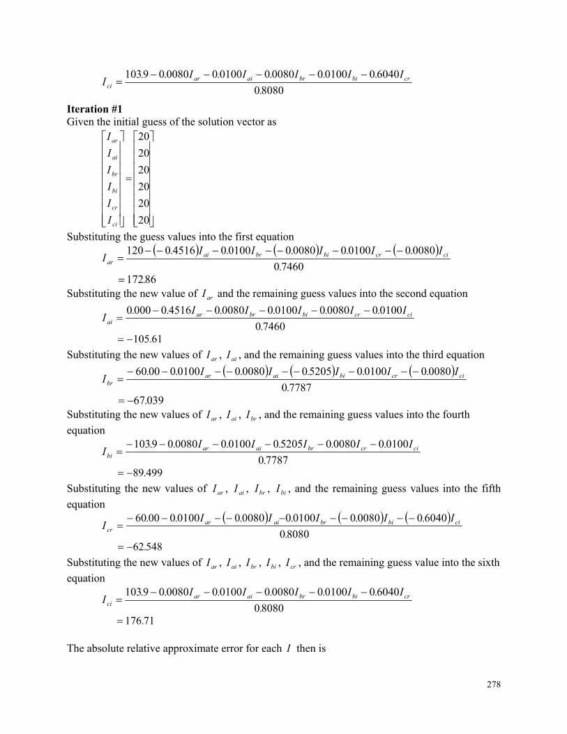
278

80800

60400010000080001000008009103

.

I.I.I.I.I..I crbibraiar

ci

Iteration #1 Given the initial guess of the solution vector as

20

20

20

20

20

20

ci

cr

bi

br

ai

ar

I

I

I

I

I

I

Substituting the guess values into the first equation

74600

0080001000008000100045160120

.

I.I.I.I.I.I cicrbibrai

ar

86172. Substituting the new value of arI and the remaining guess values into the second equation

74600

01000008000100000800451600000

.

I.I.I.I.I..I cicrbibrar

ai

61105.

Substituting the new values of arI , aiI , and the remaining guess values into the third equation

77870

00800010005205000800010000060

.

I.I.I.I.I..I cicrbiaiar

br

03967. Substituting the new values of arI , aiI , brI , and the remaining guess values into the fourth

equation

77870

01000008005205001000008009103

.

I.I.I.I.I..I cicrbraiar

bi

49989.

Substituting the new values of arI , aiI , brI , biI , and the remaining guess values into the fifth

equation

80800

60400008000100000800010000060

.

I.I.I.I.I..I cibibraiar

cr

54862.

Substituting the new values of arI , aiI , brI , biI , crI , and the remaining guess value into the sixth

equation

80800

60400010000080001000008009103

.

I.I.I.I.I..I crbibraiar

ci

71176. The absolute relative approximate error for each I then is

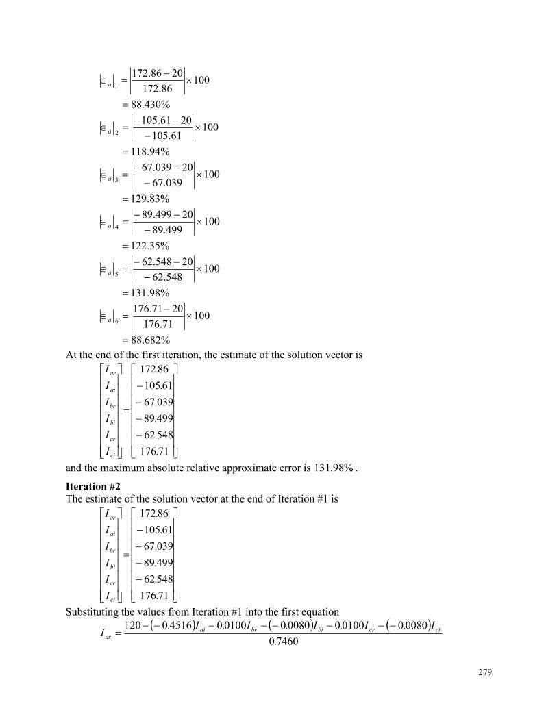
279

%430.88

10086.172

2086.1721

a

%94.118

10061.105

2061.1052

a

%83.129

100039.67

20039.673

a

%35.122

100499.89

20499.894

a

%98.131

100548.62

20548.625

a

%682.88

10071.176

2071.1766

a

At the end of the first iteration, the estimate of the solution vector is

71176

54862

49989

03967

61105

86172

.

.

.

.

.

.

I

I

I

I

I

I

ci

cr

bi

br

ai

ar

and the maximum absolute relative approximate error is %98.131 .

Iteration #2 The estimate of the solution vector at the end of Iteration #1 is

71176

54862

49989

03967

61105

86172

.

.

.

.

.

.

I

I

I

I

I

I

ci

cr

bi

br

ai

ar

Substituting the values from Iteration #1 into the first equation

74600

0080001000008000100045160120

.

I.I.I.I.I.I cicrbibrai

ar

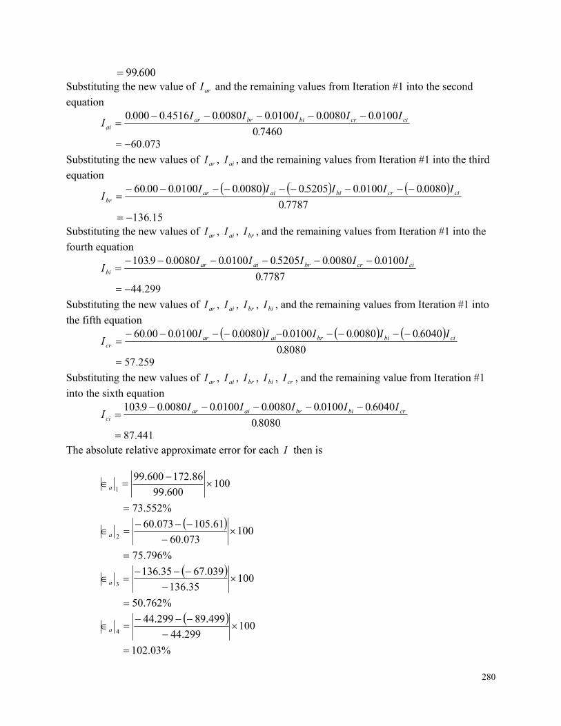
280

60099. Substituting the new value of arI and the remaining values from Iteration #1 into the second

equation

74600

01000008000100000800451600000

.

I.I.I.I.I..I cicrbibrar

ai

073.60

Substituting the new values of arI , aiI , and the remaining values from Iteration #1 into the third

equation

77870

00800010005205000800010000060

.

I.I.I.I.I..I cicrbiaiar

br

15.136 Substituting the new values of arI , aiI , brI , and the remaining values from Iteration #1 into the

fourth equation

77870

01000008005205001000008009103

.

I.I.I.I.I..I cicrbraiar

bi

299.44

Substituting the new values of arI , aiI , brI , biI , and the remaining values from Iteration #1 into

the fifth equation

80800

60400008000100000800010000060

.

I.I.I.I.I..I cibibraiar

cr

259.57

Substituting the new values of arI , aiI , brI , biI , crI , and the remaining value from Iteration #1

into the sixth equation

80800

60400010000080001000008009103

.

I.I.I.I.I..I crbibraiar

ci

441.87 The absolute relative approximate error for each I then is

%552.73

100600.99

86.172600.991

a

%796.75

100073.60

61.105073.602

a

%762.50

10035.136

039.6735.1363

a

%03.102

100299.44

499.89299.444

a

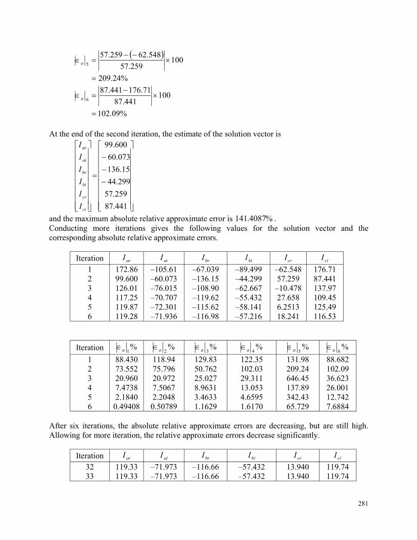
281

%24.209

100259.57

548.62259.575

a

%09.102

100441.87

71.176441.876

a

At the end of the second iteration, the estimate of the solution vector is

441.87

259.57

299.44

15.136

073.60

600.99

ci

cr

bi

br

ai

ar

I

I

I

I

I

I

and the maximum absolute relative approximate error is %4087.141 . Conducting more iterations gives the following values for the solution vector and the corresponding absolute relative approximate errors.

Iteration arI aiI brI biI crI ciI

1 2 3 4 5 6

172.86 99.600 126.01 117.25 119.87 119.28

–105.61 –60.073 –76.015 –70.707 –72.301 –71.936

–67.039 –136.15 –108.90 –119.62 –115.62 –116.98

–89.499 –44.299 –62.667 –55.432 –58.141 –57.216

–62.548 57.259 –10.478 27.658 6.2513 18.241

176.71 87.441 137.97 109.45 125.49 116.53

Iteration %1a %

2a %3a %

4a %5a %

6a

1 2 3 4 5 6

88.430 73.552 20.960 7.4738 2.1840 0.49408

118.94 75.796 20.972 7.5067 2.2048 0.50789

129.83 50.762 25.027 8.9631 3.4633 1.1629

122.35 102.03 29.311 13.053 4.6595 1.6170

131.98 209.24 646.45 137.89 342.43 65.729

88.682 102.09 36.623 26.001 12.742 7.6884

After six iterations, the absolute relative approximate errors are decreasing, but are still high. Allowing for more iteration, the relative approximate errors decrease significantly.

Iteration arI aiI brI biI crI ciI

32 33

119.33 119.33

–71.973 –71.973

–116.66 –116.66

–57.432 –57.432

13.940 13.940

119.74 119.74

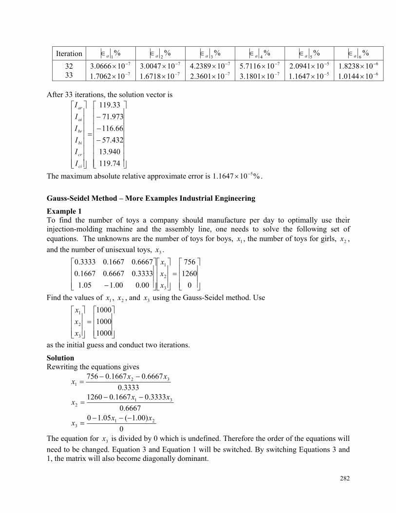
282

Iteration %1a %

2a %3a %

4a %5a %

6a

32 33

7100666.3 7107062.1

7100047.3 7106718.1

7102389.4 7103601.2

7107116.5 7101801.3

5100941.2 5101647.1

6108238.1 6100144.1

After 33 iterations, the solution vector is

74.119

940.13

432.57

66.116

973.71

33.119

ci

cr

bi

br

ai

ar

I

I

I

I

I

I

The maximum absolute relative approximate error is %101647.1 5 .

Gauss-Seidel Method – More Examples Industrial Engineering

Example 1 To find the number of toys a company should manufacture per day to optimally use their injection-molding machine and the assembly line, one needs to solve the following set of equations. The unknowns are the number of toys for boys, 1x , the number of toys for girls, 2x ,

and the number of unisexual toys, 3x .

0

1260

756

00.000.105.1

3333.06667.01667.0

6667.01667.03333.0

3

2

1

x

x

x

Find the values of 1x , 2x , and 3x using the Gauss-Seidel method. Use

1000

1000

1000

3

2

1

x

x

x

as the initial guess and conduct two iterations.

Solution Rewriting the equations gives

3333.0

6667.01667.0756 321

xxx

6667.0

3333.01667.01260 312

xxx

0

)00.1(05.10 213

xxx

The equation for 3x is divided by 0 which is undefined. Therefore the order of the equations will

need to be changed. Equation 3 and Equation 1 will be switched. By switching Equations 3 and 1, the matrix will also become diagonally dominant.

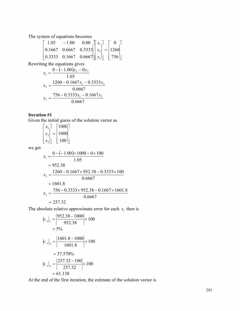
283

The system of equations becomes

756

1260

0

6667.01667.03333.0

3333.06667.01667.0

00.000.105.1

3

2

1

x

x

x

Rewriting the equations gives

05.1

000.10 321

xxx

6667.0

3333.01667.01260 312

xxx

6667.0

1667.03333.0756 213

xxx

Iteration #1 Given the initial guess of the solution vector as

100

1000

1000

3

2

1

x

x

x

we get

05.1

1000100000.101

x

38.952

6667.0

1003333.038.9521667.012602

x

8.1601

6667.0

8.16011667.038.9523333.07563

x

32.257

The absolute relative approximate error for each ix then is

10038.952

100038.9521

a

%5

1008.1601

10008.16012

a

%570.37

10032.257

10032.2573

a

138.61 At the end of the first iteration, the estimate of the solution vector is

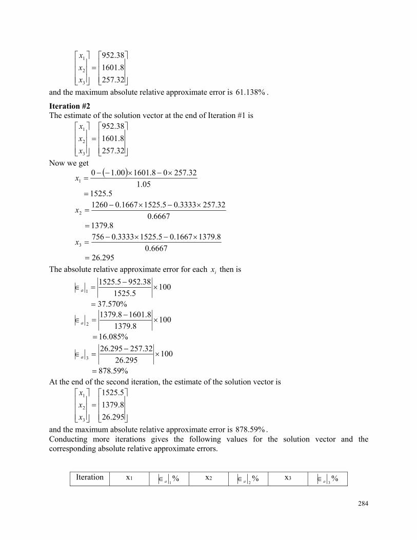
284

32.257

8.1601

38.952

3

2

1

x

x

x

and the maximum absolute relative approximate error is %138.61 .

Iteration #2 The estimate of the solution vector at the end of Iteration #1 is

32.257

8.1601

38.952

3

2

1

x

x

x

Now we get

05.1

32.25708.160100.101

x

5.1525

6667.0

32.2573333.05.15251667.012602

x

8.1379

6667.0

8.13791667.05.15253333.07563

x

295.26

The absolute relative approximate error for each ix then is

1005.1525

38.9525.15251

a

%570.37

1008.1379

8.16018.13792

a

%085.16

100295.26

32.257295.263

a

%59.878 At the end of the second iteration, the estimate of the solution vector is

295.26

8.1379

5.1525

3

2

1

x

x

x

and the maximum absolute relative approximate error is %59.878 . Conducting more iterations gives the following values for the solution vector and the corresponding absolute relative approximate errors.

Iteration x1 %1a

x2 %2a

x3 %3a

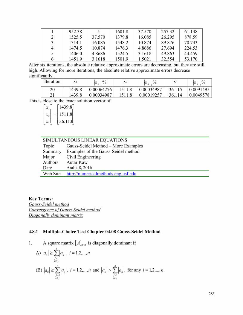
285

1 2 3 4 5 6

952.38 1525.5 1314.1 1474.5 1406.0 1451.9

5 37.570 16.085 10.874 4.8686 3.1618

1601.8 1379.8 1548.2 1476.3 1524.5 1501.9

37.570 16.085 10.874 4.8686 3.1618 1.5021

257.32 26.295 89.876 27.694 49.863 32.554

61.138 878.59 70.743 224.53 44.459 53.170

After six iterations, the absolute relative approximate errors are decreasing, but they are still high. Allowing for more iterations, the absolute relative approximate errors decrease significantly.

Iteration x1 %1a

x2 %2a

x3 %3a

20 21

1439.8 1439.8

0.00064276 0.00034987

1511.8 1511.8

0.00034987 0.00019257

36.115 36.114

0.0091495 0.0049578

This is close to the exact solution vector of

113.36

8.1511

8.1439

3

2

1

x

x

x

SIMULTANEOUS LINEAR EQUATIONS Topic Gauss-Seidel Method – More Examples Summary Examples of the Gauss-Seidel method Major Civil Engineering Authors Autar Kaw Date Aralık 8, 2016 Web Site http://numericalmethods.eng.usf.edu

Key Terms: Gauss-Seidel method Convergence of Gauss-Seidel method Diagonally dominant matrix 4.8.1 Multiple-Choice Test Chapter 04.08 Gauss-Seidel Method 1. A square matrix nnA is diagonally dominant if

A) ,1

n

jij

ijii aa ni ,...,2,1

(B) ,1

n

jij

ijii aa ni ,...,2,1 and ,1

n

jij

ijii aa for any ni ,...,2,1

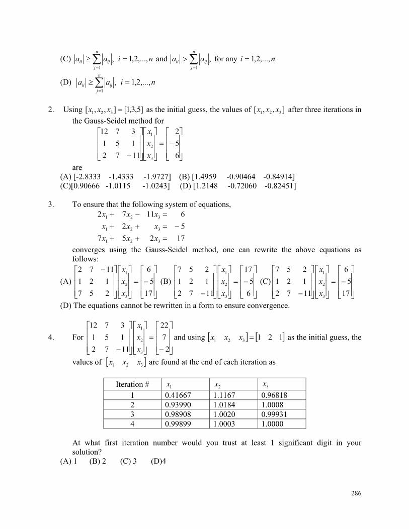
286

(C) ,1

n

jijii aa ni ,...,2,1 and ,

1

n

jijii aa for any ni ,...,2,1

(D) ,1

n

jijii aa ni ,...,2,1

2. Using ]5,3,1[],,[ 321 xxx as the initial guess, the values of ],,[ 321 xxx after three iterations in

the Gauss-Seidel method for

6

5

2

1172

151

3712

3

2

1

x

x

x

are (A) [-2.8333 -1.4333 -1.9727] (B) [1.4959 -0.90464 -0.84914] (C)[0.90666 -1.0115 -1.0243] (D) [1.2148 -0.72060 -0.82451]

3. To ensure that the following system of equations,

17257

52

61172

321

321

321

xxx

xxx

xxx

converges using the Gauss-Seidel method, one can rewrite the above equations as follows:

(A)

17

5

6

257

121

1172

3

2

1

x

x

x

(B)

6

5

17

1172

121

257

3

2

1

x

x

x

(C)

17

5

6

1172

121

257

3

2

1

x

x

x

(D) The equations cannot be rewritten in a form to ensure convergence.

4. For

2

7

22

1172

151

3712

3

2

1

x

x

x

and using 121321 xxx as the initial guess, the

values of 321 xxx are found at the end of each iteration as

Iteration # 1x 2x 3x

1 0.41667 1.1167 0.96818 2 0.93990 1.0184 1.0008 3 0.98908 1.0020 0.99931 4 0.99899 1.0003 1.0000

At what first iteration number would you trust at least 1 significant digit in your solution?

(A) 1 (B) 2 (C) 3 (D)4

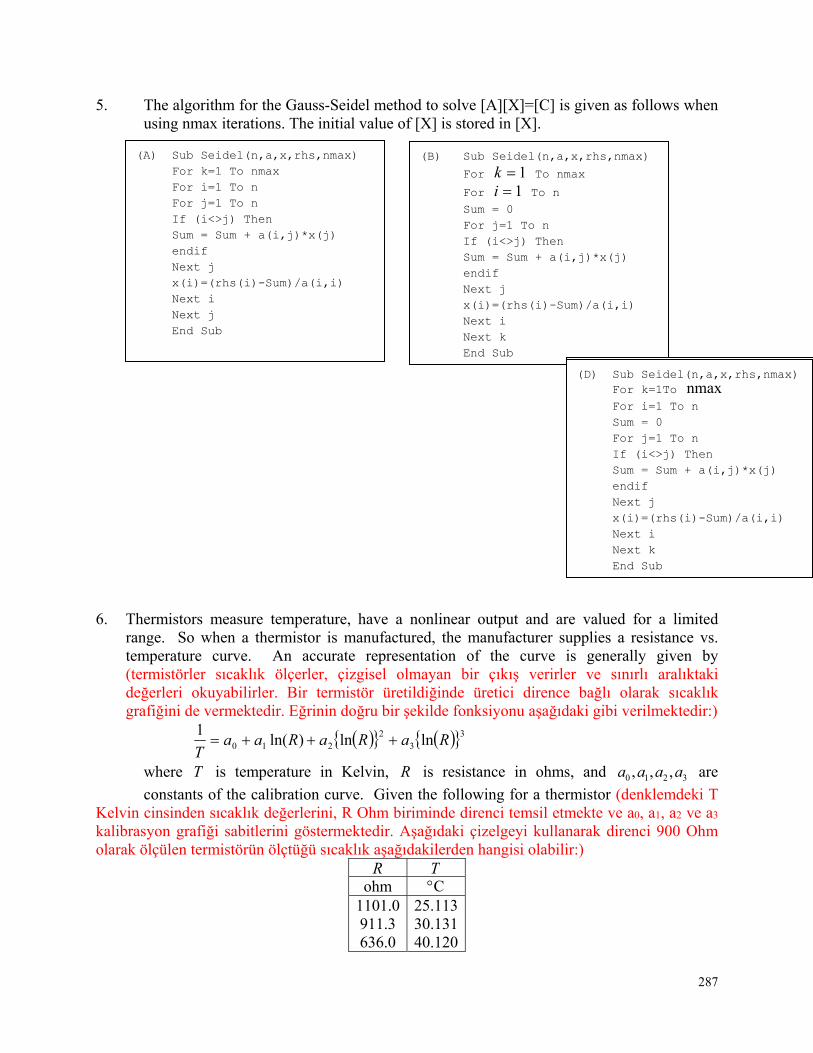
287

5. The algorithm for the Gauss-Seidel method to solve [A][X]=[C] is given as follows when using nmax iterations. The initial value of [X] is stored in [X].

6. Thermistors measure temperature, have a nonlinear output and are valued for a limited

range. So when a thermistor is manufactured, the manufacturer supplies a resistance vs. temperature curve. An accurate representation of the curve is generally given by (termistörler sıcaklık ölçerler, çizgisel olmayan bir çıkış verirler ve sınırlı aralıktaki değerleri okuyabilirler. Bir termistör üretildiğinde üretici dirence bağlı olarak sıcaklık grafiğini de vermektedir. Eğrinin doğru bir şekilde fonksiyonu aşağıdaki gibi verilmektedir:)

3

32

210 lnln)ln(1

RaRaRaaT

where T is temperature in Kelvin, R is resistance in ohms, and 3210 ,,, aaaa are

constants of the calibration curve. Given the following for a thermistor (denklemdeki T Kelvin cinsinden sıcaklık değerlerini, R Ohm biriminde direnci temsil etmekte ve a0, a1, a2 ve a3 kalibrasyon grafiği sabitlerini göstermektedir. Aşağıdaki çizelgeyi kullanarak direnci 900 Ohm olarak ölçülen termistörün ölçtüğü sıcaklık aşağıdakilerden hangisi olabilir:)

R T ohm C

1101.0 911.3 636.0

25.113 30.131 40.120

(A) Sub Seidel(n,a,x,rhs,nmax) For k=1 To nmax For i=1 To n For j=1 To n If (i<>j) Then Sum = Sum + a(i,j)*x(j) endif Next j x(i)=(rhs(i)-Sum)/a(i,i) Next i Next j End Sub

(B) Sub Seidel(n,a,x,rhs,nmax)

For 1k To nmax

For 1i To n Sum = 0 For j=1 To n If (i<>j) Then Sum = Sum + a(i,j)*x(j) endif Next j x(i)=(rhs(i)-Sum)/a(i,i) Next i Next k End Sub

(C) Sub Seidel(n,a,x,rhs,nmax) For k=1 To nmax For i=1 To n Sum = 0 For j=1 To n Sum = Sum + a(i,j)*x(j) Next j x(i)=(rhs(i)-Sum)/a(i,i) Next i Next k End Sub

(D) Sub Seidel(n,a,x,rhs,nmax) For k=1To nmax For i=1 To n Sum = 0 For j=1 To n If (i<>j) Then Sum = Sum + a(i,j)*x(j) endif Next j x(i)=(rhs(i)-Sum)/a(i,i) Next i Next k End Sub

288

451.1 50.128 the value of temperature in C for a measured resistance of 900 ohms most nearly is

(A) 30.002 (B) 30.473 (C) 31.272 (D) 31.445 For a complete solution, refer to the links at the end of the book.

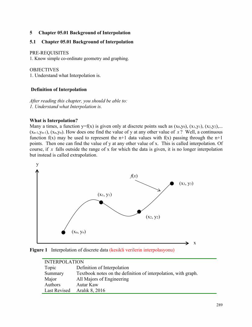
289

5 Chapter 05.01 Background of Interpolation

5.1 Chapter 05.01 Background of Interpolation PRE-REQUISITES 1. Know simple co-ordinate geometry and graphing.

OBJECTIVES 1. Understand what Interpolation is.

Definition of Interpolation After reading this chapter, you should be able to: 1. Understand what Interpolation is.

What is Interpolation? Many a times, a function y=f(x) is given only at discrete points such as (x0,y0), (x1,y1), (x2,y2),... (xn-1,yn-1), (xn,yn). How does one find the value of y at any other value of x ? Well, a continuous function f(x) may be used to represent the n+1 data values with f(x) passing through the n+1 points. Then one can find the value of y at any other value of x. This is called interpolation. Of course, if x falls outside the range of x for which the data is given, it is no longer interpolation but instead is called extrapolation.

Figure 1 Interpolation of discrete data (kesikli verilerin interpolasyonu)

INTERPOLATION Topic Definition of Interpolation Summary Textbook notes on the definition of interpolation, with graph. Major All Majors of Engineering Authors Autar Kaw Last Revised Aralık 8, 2016

(xo, yo)

(x1, y1)

(x2, y2)

(x3, y3)

y

x

f(x)

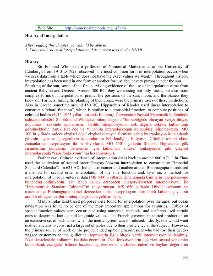
290

Web Site http://numericalmethods.eng.usf.edu

History of Interpolation After reading this chapter, you should be able to: 1. Know the history of Interpolation and its current uses by the HNMI.

History Sir Edmund Whittaker, a professor of Numerical Mathematics at the University of Edinburgh from 1913 to 1923, observed “the most common form of interpolation occurs when we seek data from a table which does not have the exact values we want.” Throughout history, interpolation has been used in one form or another for just about every purpose under the sun. Speaking of the sun, some of the first surviving evidence of the use of interpolation came from ancient Babylon and Greece. Around 300 BC, they were using not only linear, but also more complex forms of interpolation to predict the positions of the sun, moon, and the planets they knew of. Farmers, timing the planting of their crops, were the primary users of these predictions. Also in Greece sometime around 150 BC, Hipparchus of Rhodes used linear interpolation to construct a “chord function”, which is similar to a sinusoidal function, to compute positions of celestial bodies (1913-1923 yılları arasında Edinburg Üniversitesi Sayısal Matematik bölümünde çalışan profesörü Sir Edmund Whittaker interpolasyonu “bir çizelgede olmayan veriye ihtiyaç duyulması” şeklinde açıklamıştır. Tarihte interpolasyonun çok değişik şekilde kullanıldığı görülmektedir. Antik Babil’de ve Yunan’da interpolasyonun kullanıldığı bilinmektedir. MÖ 300’lü yıllarda sadece çizgisel değil çizgisel olmayan formlara sahip interpolasyon kullanılarak güneşin, ayın ve gezegenlerin konumlarının belirlendiğini biliyoruz. Çiftçiler tohum ekme zamanlarını interpolasyon ile belirliyorlardı. MÖ 150’li yıllarda Rodoslu Hipparchus gök cisimlerinin konularını belirlemek için kullanılan sinüsel fonksiyonlar gibi çizgisel interpolasyonla “akor fonksiyonu” 'nu hesaplıyordu.). Farther east, Chinese evidence of interpolation dates back to around 600 AD. Liu Zhuo used the equivalent of second order Gregory-Newton interpolation to construct an “Imperial Standard Calendar”. In 625 AD, Indian astronomer and mathematician Brahmagupta introduced a method for second order interpolation of the sine function and, later on, a method for interpolation of unequal-interval data (MS 600’lü yıllarda daha doğuda Çinlilerin interpolasyonu kullandığı biliniyordu. Liu Zhuo ikinci dereceden Gregory-Newton interpolasyonu ile “İmparatorluk Standart Takvimi”’ni oluşturmuştu. MS 650 yıllarda Hindli astronom ve matematikçi Brahmagupta ikinci dereceden sinüs interpolasyon formülünü kullanmış ve eşit aralıklı olmayan verilerin interpolasyonunu geliştirmiştir.). Many similar land-based purposes were found for interpolation over the ages, but ocean navigation was found to be one of the most important applications for centuries. Tables of special function values were constructed using numerical methods, and seafarers used certain ones to determine latitude and longitude values. The French government started production on an extensive set of such tables when the metric system was introduced. Ideally, one would want mathematicians to construct a large set of tables due to their proficiency at the subject. However, the primary source of work on the project ended up being hairdressers who had lost their gaudy-wigged customers to the guillotine (topraklarla ilgili birçok yerde interpolasyon kullanılmış, fakat denizlerdeki kullanımı ise daha önemlidir. Özel fonksiyonların değerleri sayısal yöntemler kullanılarak çizelgeler halinde hazırlanmış, denizciler tarafından enlem ve boylam değerlerini

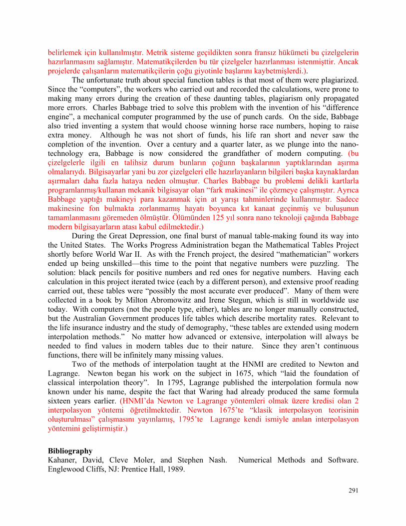
291

belirlemek için kullanılmıştır. Metrik sisteme geçildikten sonra fransız hükümeti bu çizelgelerin hazırlanmasını sağlamıştır. Matematikçilerden bu tür çizelgeler hazırlanması istenmişttir. Ancak projelerde çalışanların matematikçilerin çoğu giyotinle başlarını kaybetmişlerdi.). The unfortunate truth about special function tables is that most of them were plagiarized. Since the “computers”, the workers who carried out and recorded the calculations, were prone to making many errors during the creation of these daunting tables, plagiarism only propagated more errors. Charles Babbage tried to solve this problem with the invention of his “difference engine”, a mechanical computer programmed by the use of punch cards. On the side, Babbage also tried inventing a system that would choose winning horse race numbers, hoping to raise extra money. Although he was not short of funds, his life ran short and never saw the completion of the invention. Over a century and a quarter later, as we plunge into the nano-technology era, Babbage is now considered the grandfather of modern computing. (bu çizelgelerle ilgili en talihsiz durum bunların çoğunn başkalarının yaptıklarından aşırma olmalarıydı. Bilgisayarlar yani bu zor çizelgeleri elle hazırlayanların bilgileri başka kaynaklardan aşırmaları daha fazla hataya neden olmuştur. Charles Babbage bu problemi delikli kartlarla programlanmış/kullanan mekanik bilgisayar olan “fark makinesi” ile çözmeye çalışmıştır. Ayrıca Babbage yaptığı makineyi para kazanmak için at yarışı tahminlerinde kullanmıştır. Sadece makinesine fon bulmakta zorlanmamış hayatı boyunca kıt kanaat geçinmiş ve buluşunun tamamlanmasını göremeden ölmüştür. Ölümünden 125 yıl sonra nano teknoloji çağında Babbage modern bilgisayarların atası kabul edilmektedir.) During the Great Depression, one final burst of manual table-making found its way into the United States. The Works Progress Administration began the Mathematical Tables Project shortly before World War II. As with the French project, the desired “mathematician” workers ended up being unskilled—this time to the point that negative numbers were puzzling. The solution: black pencils for positive numbers and red ones for negative numbers. Having each calculation in this project iterated twice (each by a different person), and extensive proof reading carried out, these tables were “possibly the most accurate ever produced”. Many of them were collected in a book by Milton Abromowitz and Irene Stegun, which is still in worldwide use today. With computers (not the people type, either), tables are no longer manually constructed, but the Australian Government produces life tables which describe mortality rates. Relevant to the life insurance industry and the study of demography, “these tables are extended using modern interpolation methods.” No matter how advanced or extensive, interpolation will always be needed to find values in modern tables due to their nature. Since they aren’t continuous functions, there will be infinitely many missing values. Two of the methods of interpolation taught at the HNMI are credited to Newton and Lagrange. Newton began his work on the subject in 1675, which “laid the foundation of classical interpolation theory”. In 1795, Lagrange published the interpolation formula now known under his name, despite the fact that Waring had already produced the same formula sixteen years earlier. (HNMI’da Newton ve Lagrange yöntemleri olmak üzere kredisi olan 2 interpolasyon yöntemi öğretilmektedir. Newton 1675’te “klasik interpolasyon teorisinin oluşturulması” çalışmasını yayınlamış, 1795’te Lagrange kendi ismiyle anılan interpolasyon yöntemini geliştirmiştir.)

Bibliography Kahaner, David, Cleve Moler, and Stephen Nash. Numerical Methods and Software. Englewood Cliffs, NJ: Prentice Hall, 1989.

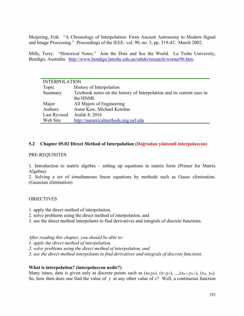
292

Meijering, Erik. “A Chronology of Interpolation: From Ancient Astronomy to Modern Signal and Image Processing.” Proceedings of the IEEE. vol. 90, no. 3, pp. 319-42. March 2002. Mills, Terry. “Historical Notes.” Join the Dots and See the World. La Trobe University, Bendigo, Australia. http://www.bendigo.latrobe.edu.au/rahdo/research/worner96.htm.

INTERPOLATION Topic History of Interpolation Summary Textbook notes on the history of Interpolation and its current uses in

the HNMI. Major All Majors of Engineering Authors Autar Kaw, Michael Keteltas Last Revised Aralık 8, 2016 Web Site http://numericalmethods.eng.usf.edu

5.2 Chapter 05.02 Direct Method of Interpolation (Doğrudan yöntemli interpolasyon)

PRE-REQUISITES

1. Introduction to matrix algebra – setting up equations in matrix form (Primer for Matrix Algebra). 2. Solving a set of simultaneous linear equations by methods such as Gauss elimination. (Gaussian elimination)

OBJECTIVES

1. apply the direct method of interpolation, 2. solve problems using the direct method of interpolation, and 3. use the direct method interpolants to find derivatives and integrals of discrete functions. After reading this chapter, you should be able to: 1. apply the direct method of interpolation, 2. solve problems using the direct method of interpolation, and 3. use the direct method interpolants to find derivatives and integrals of discrete functions.

What is interpolation? (interpolasyon nedir?) Many times, data is given only at discrete points such as (x0,y0), (x1,y1), ...,(xn-1,yn-1), (xn, yn). So, how then does one find the value of y at any other value of x? Well, a continuous function

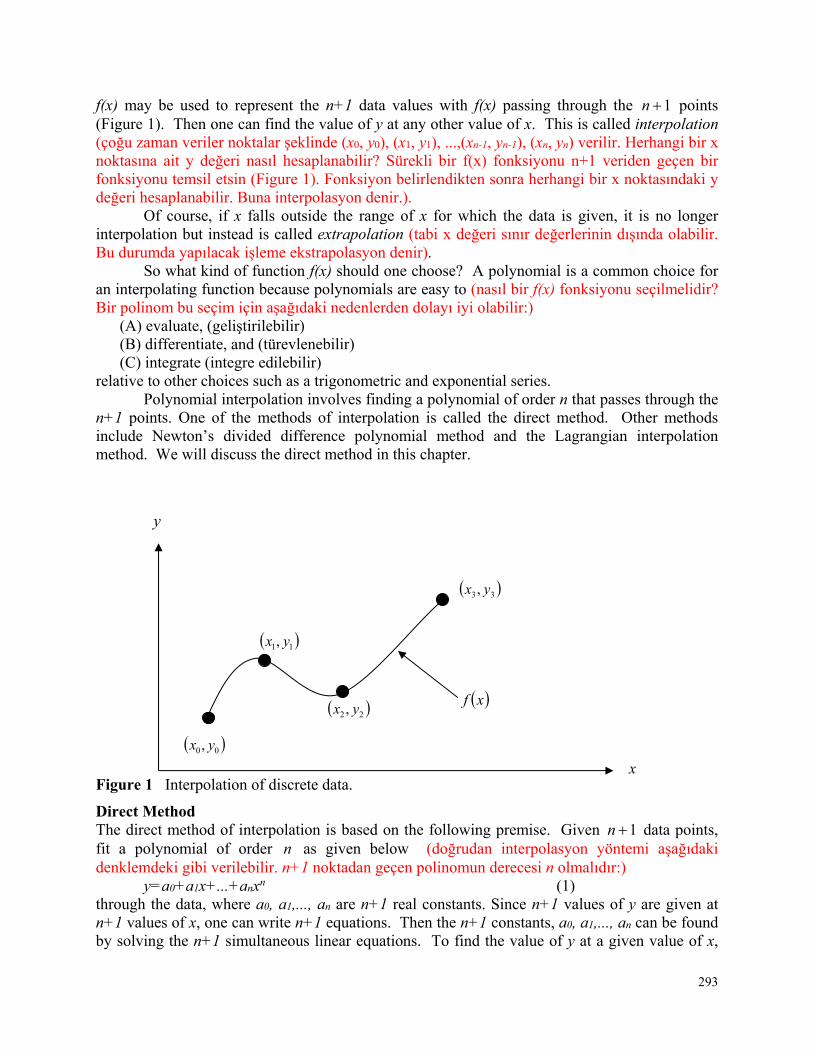
293

f(x) may be used to represent the n+1 data values with f(x) passing through the 1n points (Figure 1). Then one can find the value of y at any other value of x. This is called interpolation (çoğu zaman veriler noktalar şeklinde (x0, y0), (x1, y1), ...,(xn-1, yn-1), (xn, yn) verilir. Herhangi bir x noktasına ait y değeri nasıl hesaplanabilir? Sürekli bir f(x) fonksiyonu n+1 veriden geçen bir fonksiyonu temsil etsin (Figure 1). Fonksiyon belirlendikten sonra herhangi bir x noktasındaki y değeri hesaplanabilir. Buna interpolasyon denir.). Of course, if x falls outside the range of x for which the data is given, it is no longer interpolation but instead is called extrapolation (tabi x değeri sınır değerlerinin dışında olabilir. Bu durumda yapılacak işleme ekstrapolasyon denir). So what kind of function f(x) should one choose? A polynomial is a common choice for an interpolating function because polynomials are easy to (nasıl bir f(x) fonksiyonu seçilmelidir? Bir polinom bu seçim için aşağıdaki nedenlerden dolayı iyi olabilir:)

(A) evaluate, (geliştirilebilir) (B) differentiate, and (türevlenebilir) (C) integrate (integre edilebilir)

relative to other choices such as a trigonometric and exponential series. Polynomial interpolation involves finding a polynomial of order n that passes through the n+1 points. One of the methods of interpolation is called the direct method. Other methods include Newton’s divided difference polynomial method and the Lagrangian interpolation method. We will discuss the direct method in this chapter. Figure 1 Interpolation of discrete data.

Direct Method The direct method of interpolation is based on the following premise. Given 1n data points, fit a polynomial of order n as given below (doğrudan interpolasyon yöntemi aşağıdaki denklemdeki gibi verilebilir. n+1 noktadan geçen polinomun derecesi n olmalıdır:) y=a0+a1x+...+anxn (1) through the data, where a0, a1,..., an are n+1 real constants. Since n+1 values of y are given at n+1 values of x, one can write n+1 equations. Then the n+1 constants, a0, a1,..., an can be found by solving the n+1 simultaneous linear equations. To find the value of y at a given value of x,

00, yx

11, yx

22 , yx

33, yx

xf

x

y

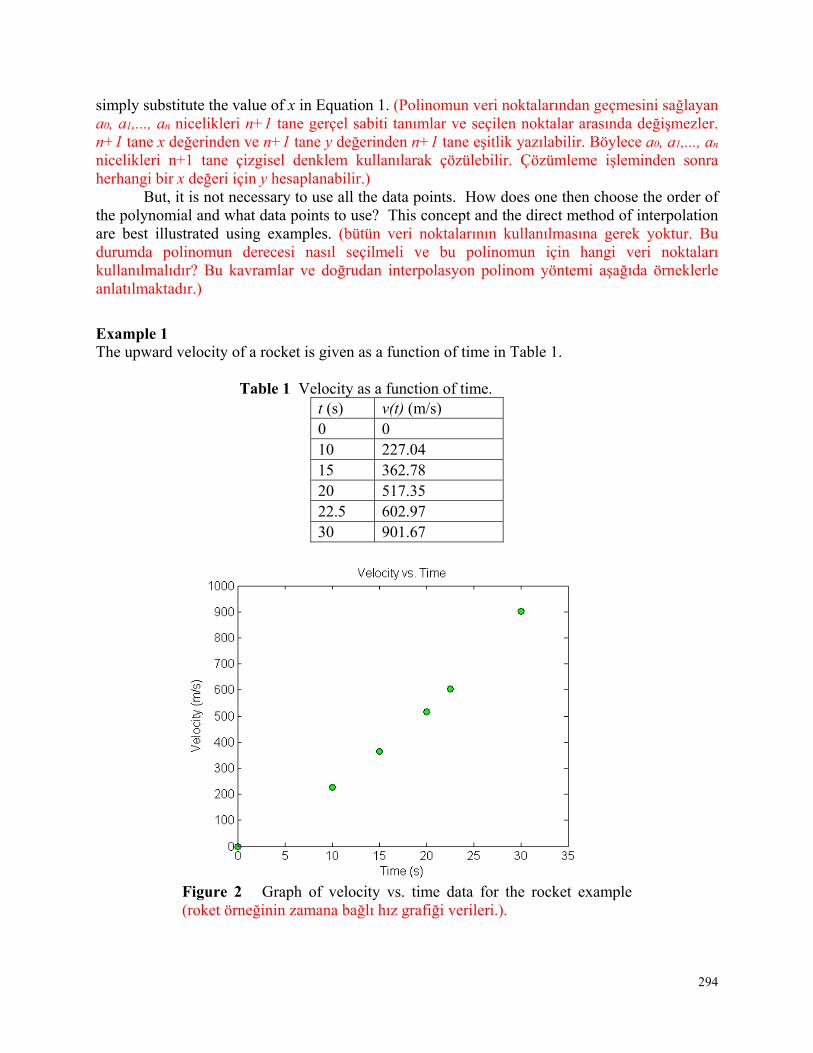
294

simply substitute the value of x in Equation 1. (Polinomun veri noktalarından geçmesini sağlayan a0, a1,..., an nicelikleri n+1 tane gerçel sabiti tanımlar ve seçilen noktalar arasında değişmezler. n+1 tane x değerinden ve n+1 tane y değerinden n+1 tane eşitlik yazılabilir. Böylece a0, a1,..., an nicelikleri n+1 tane çizgisel denklem kullanılarak çözülebilir. Çözümleme işleminden sonra herhangi bir x değeri için y hesaplanabilir.) But, it is not necessary to use all the data points. How does one then choose the order of the polynomial and what data points to use? This concept and the direct method of interpolation are best illustrated using examples. (bütün veri noktalarının kullanılmasına gerek yoktur. Bu durumda polinomun derecesi nasıl seçilmeli ve bu polinomun için hangi veri noktaları kullanılmalıdır? Bu kavramlar ve doğrudan interpolasyon polinom yöntemi aşağıda örneklerle anlatılmaktadır.)

Example 1 The upward velocity of a rocket is given as a function of time in Table 1.

Table 1 Velocity as a function of time. t (s) v(t) (m/s) 0 0 10 227.04 15 362.78 20 517.35 22.5 602.97 30 901.67

Figure 2 Graph of velocity vs. time data for the rocket example (roket örneğinin zamana bağlı hız grafiği verileri.).

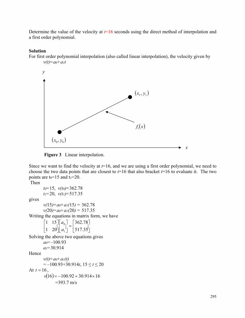
295

Determine the value of the velocity at t=16 seconds using the direct method of interpolation and a first order polynomial.

Solution For first order polynomial interpolation (also called linear interpolation), the velocity given by v(t)=a0+a1t

Figure 3 Linear interpolation.

Since we want to find the velocity at t=16, and we are using a first order polynomial, we need to choose the two data points that are closest to t=16 that also bracket t=16 to evaluate it. The two points are t0=15 and t1=20. Then t0=15, v(t0)=362.78 t1=20, v(t1)=517.35 gives v(15)=a0+a1(15) = 362.78 v(20)=a0+a1(20) = 517.35 Writing the equations in matrix form, we have

35.517

78.362

201

151

1

0

a

a

Solving the above two equations gives a0=–100.93 a1=30.914 Hence v(t)=a0+a1(t) = –100.93+30.914t, 15 ≤ t ≤ 20 At 16t , 16914.3092.10016 v =393.7 m/s

00, yx

11, yx

xf1

x

y

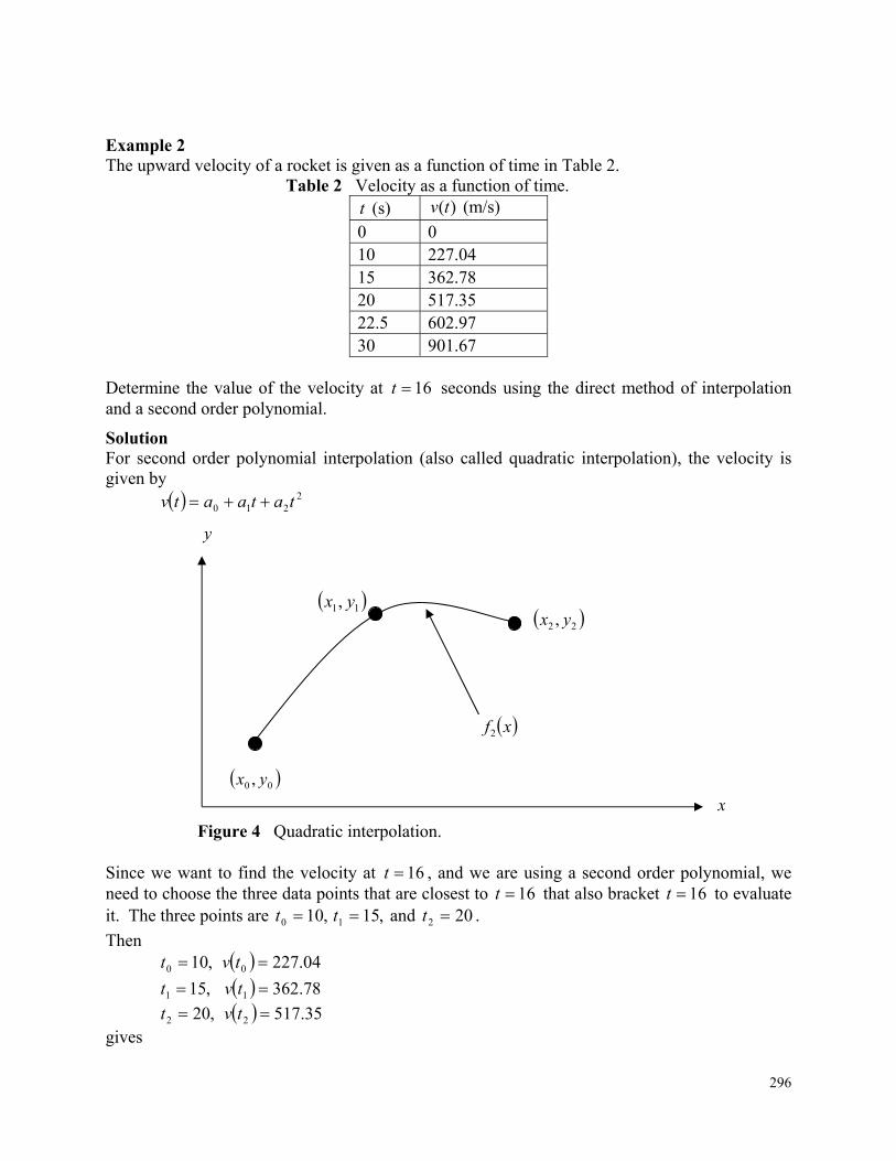
296

Example 2 The upward velocity of a rocket is given as a function of time in Table 2.

Table 2 Velocity as a function of time. t (s) )(tv (m/s)

0 0 10 227.04 15 362.78 20 517.35 22.5 602.97 30 901.67

Determine the value of the velocity at 16t seconds using the direct method of interpolation and a second order polynomial.

Solution For second order polynomial interpolation (also called quadratic interpolation), the velocity is given by 2

210 tataatv

Figure 4 Quadratic interpolation.

Since we want to find the velocity at 16t , and we are using a second order polynomial, we need to choose the three data points that are closest to 16t that also bracket 16t to evaluate it. The three points are 20 and ,15,10 210 ttt .

Then 04.227,10 00 tvt

78.362 ,15 11 tvt

35.517,20 22 tvt gives

00 , yx

11, yx 22 , yx

xf2

y

x

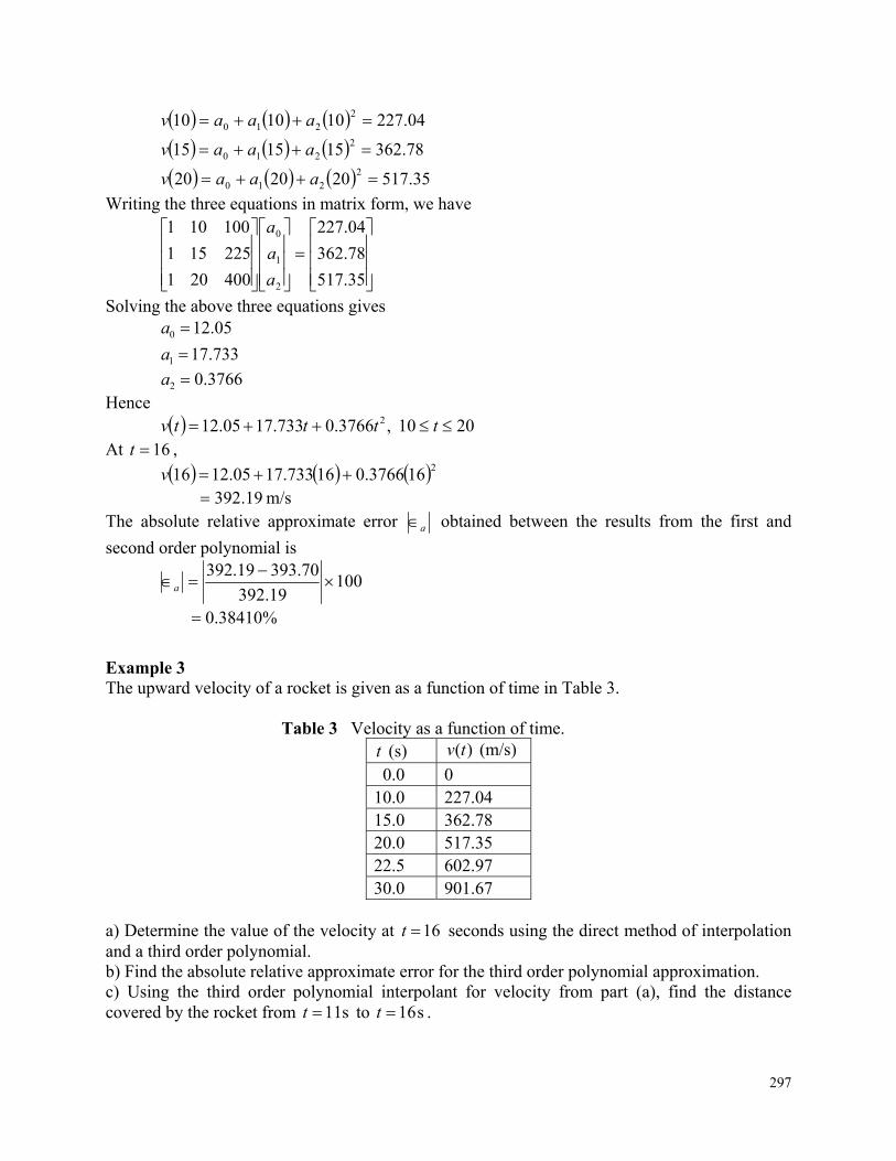
297

04.227101010 2210 aaav

78.362151515 2210 aaav

35.517202020 2210 aaav

Writing the three equations in matrix form, we have

35.517

78.362

04.227

400201

225151

100101

2

1

0

a

a

a

Solving the above three equations gives 05.120 a

733.171 a

3766.02 a Hence 2010,3766.0733.1705.12 2 ttttv At 16t ,

2163766.016733.1705.1216 v m/s 19.392 The absolute relative approximate error a obtained between the results from the first and

second order polynomial is

10019.392

70.39319.392

a

%38410.0

Example 3 The upward velocity of a rocket is given as a function of time in Table 3.

Table 3 Velocity as a function of time. t (s) )(tv (m/s)

0.0 0 10.0 227.04 15.0 362.78 20.0 517.35 22.5 602.97 30.0 901.67

a) Determine the value of the velocity at 16t seconds using the direct method of interpolation and a third order polynomial. b) Find the absolute relative approximate error for the third order polynomial approximation. c) Using the third order polynomial interpolant for velocity from part (a), find the distance covered by the rocket from s11t to s16t .

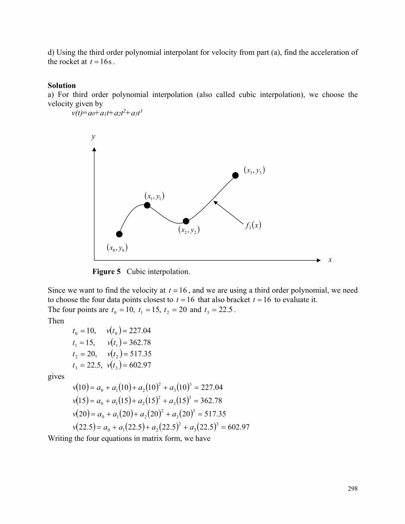
298

d) Using the third order polynomial interpolant for velocity from part (a), find the acceleration of the rocket at s16t .

Solution a) For third order polynomial interpolation (also called cubic interpolation), we choose the velocity given by v(t)=a0+a1t+a2t2+a3t3

Figure 5 Cubic interpolation. Since we want to find the velocity at 16t , and we are using a third order polynomial, we need to choose the four data points closest to 16t that also bracket 16t to evaluate it. The four points are 20 ,15 ,10 210 ttt and 5.223 t .

Then 04.227 ,10 00 tvt

78.362 ,15 11 tvt

35.517 ,20 22 tvt

97.602,5.22 33 tvt

gives

04.22710101010 33

2210 aaaav

78.36215151515 33

2210 aaaav

35.51720202020 33

2210 aaaav

97.6025.225.225.225.22 33

2210 aaaav

Writing the four equations in matrix form, we have

00, yx

11, yx

22 , yx

33, yx

xf3

x

y

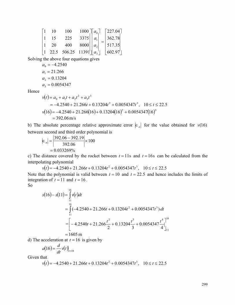
299

97.602

35.517

78.362

04.227

1139125.5065.221

8000400201

3375225151

1000100101

3

2

1

0

a

a

a

a

Solving the above four equations gives 2540.40 a

266.211 a

13204.02 a

0054347.03 a

Hence 3

32

210 tatataatv

5.2210,0054347.013204.0266.212540.4 32 tttt

32 160054347.01613204.016266.212540.416 v m/s06.392

b) The absolute percentage relative approximate error a for the value obtained for )16(v

between second and third order polynomial is

10006.392

19.39206.392

a

%033269.0 c) The distance covered by the rocket between s11t and s16t can be calculated from the interpolating polynomial 5.2210,0054347.013204.0266.212540.4 32 tttttv Note that the polynomial is valid between 10t and 5.22t and hence includes the limits of integration of 11t and 16t . So

16

11

1116 dttvss

dtttt 16

11

32 )0054347.013204.0266.212540.4(

=16

11

432

40054347.0

313204.0

2266.212540.4

tttt

m 1605 d) The acceleration at 16t is given by

16

16

t

tvdt

da

Given that 5.2210,0054347.013204.0266.212540.4 32 tttttv

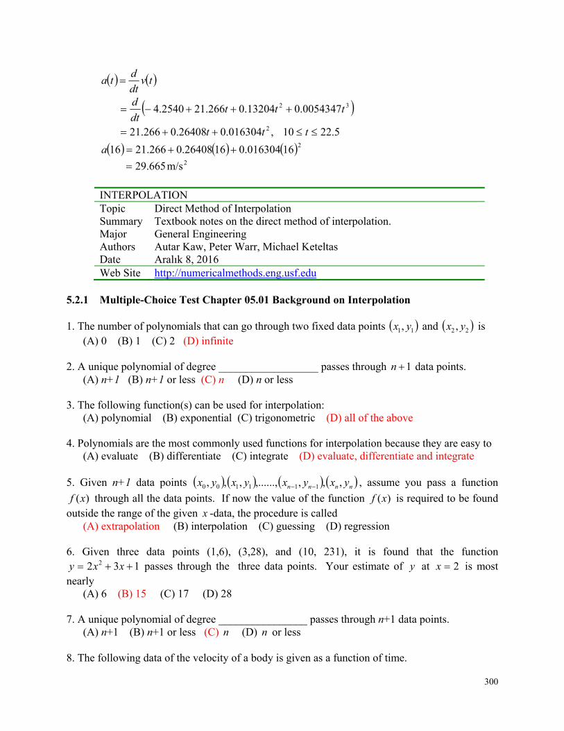
300

tvdt

dta

32 0054347.013204.0266.212540.4 tttdt

d

5.2210,016304.026408.0266.21 2 ttt

216016304.01626408.0266.2116 a

2m/s665.29

INTERPOLATION Topic Direct Method of Interpolation Summary Textbook notes on the direct method of interpolation. Major General Engineering Authors Autar Kaw, Peter Warr, Michael Keteltas Date Aralık 8, 2016 Web Site http://numericalmethods.eng.usf.edu

5.2.1 Multiple-Choice Test Chapter 05.01 Background on Interpolation 1. The number of polynomials that can go through two fixed data points 11, yx and 22 , yx is

(A) 0 (B) 1 (C) 2 (D) infinite 2. A unique polynomial of degree __________________ passes through 1n data points.

(A) n+1 (B) n+1 or less (C) n (D) n or less 3. The following function(s) can be used for interpolation:

(A) polynomial (B) exponential (C) trigonometric (D) all of the above 4. Polynomials are the most commonly used functions for interpolation because they are easy to

(A) evaluate (B) differentiate (C) integrate (D) evaluate, differentiate and integrate 5. Given n+1 data points nnnn yxyxyxyx ,,,,......,,,, 111100 , assume you pass a function

)(xf through all the data points. If now the value of the function )(xf is required to be found outside the range of the given x -data, the procedure is called

(A) extrapolation (B) interpolation (C) guessing (D) regression

6. Given three data points (1,6), (3,28), and (10, 231), it is found that the function 132 2 xxy passes through the three data points. Your estimate of y at 2x is most

nearly (A) 6 (B) 15 (C) 17 (D) 28

7. A unique polynomial of degree ________________ passes through n+1 data points.

(A) n+1 (B) n+1 or less (C) n (D) n or less 8. The following data of the velocity of a body is given as a function of time.

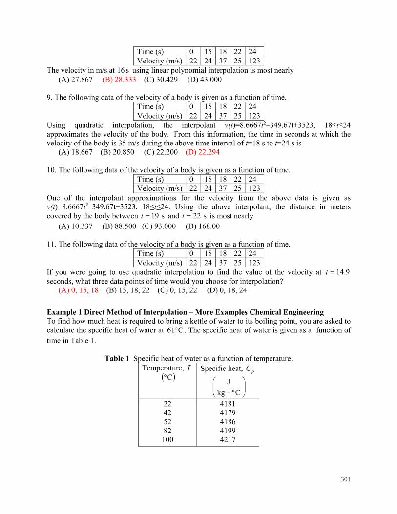
301

Time (s) 0 15 18 22 24 Velocity (m/s) 22 24 37 25 123

The velocity in m/s at s 16 using linear polynomial interpolation is most nearly (A) 27.867 (B) 28.333 (C) 30.429 (D) 43.000

9. The following data of the velocity of a body is given as a function of time.

Time (s) 0 15 18 22 24 Velocity (m/s) 22 24 37 25 123

Using quadratic interpolation, the interpolant v(t)=8.6667t2–349.67t+3523, 18≤t≤24 approximates the velocity of the body. From this information, the time in seconds at which the velocity of the body is 35 m/s during the above time interval of t=18 s to t=24 s is

(A) 18.667 (B) 20.850 (C) 22.200 (D) 22.294 10. The following data of the velocity of a body is given as a function of time.

Time (s) 0 15 18 22 24 Velocity (m/s) 22 24 37 25 123

One of the interpolant approximations for the velocity from the above data is given as v(t)=8.6667t2–349.67t+3523, 18≤t≤24. Using the above interpolant, the distance in meters covered by the body between s 19t and s 22t is most nearly

(A) 10.337 (B) 88.500 (C) 93.000 (D) 168.00 11. The following data of the velocity of a body is given as a function of time.

Time (s) 0 15 18 22 24 Velocity (m/s) 22 24 37 25 123

If you were going to use quadratic interpolation to find the value of the velocity at 9.14t seconds, what three data points of time would you choose for interpolation?

(A) 0, 15, 18 (B) 15, 18, 22 (C) 0, 15, 22 (D) 0, 18, 24

Example 1 Direct Method of Interpolation – More Examples Chemical Engineering To find how much heat is required to bring a kettle of water to its boiling point, you are asked to calculate the specific heat of water at C61 . The specific heat of water is given as a function of time in Table 1.

Table 1 Specific heat of water as a function of temperature. Temperature, T

C Specific heat, pC

Ckg

J

22 42 52 82 100

4181 4179 4186 4199 4217

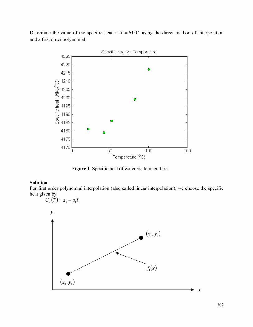
302

Determine the value of the specific heat at C61T using the direct method of interpolation and a first order polynomial.

Figure 1 Specific heat of water vs. temperature.

Solution For first order polynomial interpolation (also called linear interpolation), we choose the specific heat given by TaaTC p 10

00, yx

11, yx

xf1

x

y

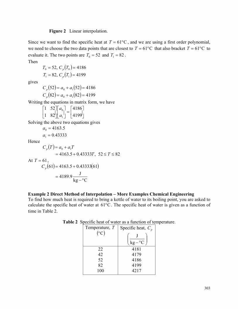
303

Figure 2 Linear interpolation. Since we want to find the specific heat at C61T , and we are using a first order polynomial, we need to choose the two data points that are closest to C61T that also bracket C61T to

evaluate it. The two points are 520 T and 821 T .

Then 4186,52 00 TCT p

4199,82 11 TCT p

gives

41865252 10 aaC p

41998282 10 aaC p

Writing the equations in matrix form, we have

4199

4186

821

521

1

0

a

a

Solving the above two equations gives 5.41630 a

43333.01 a Hence TaaTC p 10

8252,43333.05.4163 TT At 61T , 6143333.05.416361 pC

Ckg

J9.4189

Example 2 Direct Method of Interpolation – More Examples Chemical Engineering To find how much heat is required to bring a kettle of water to its boiling point, you are asked to calculate the specific heat of water at C61 . The specific heat of water is given as a function of time in Table 2.

Table 2 Specific heat of water as a function of temperature. Temperature, T

C Specific heat, pC

Ckg

J

22 42 52 82 100

4181 4179 4186 4199 4217

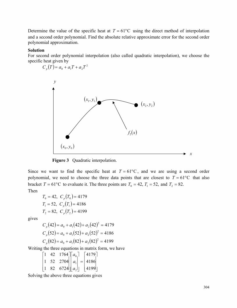
304

Determine the value of the specific heat at C61T using the direct method of interpolation and a second order polynomial. Find the absolute relative approximate error for the second order polynomial approximation.

Solution For second order polynomial interpolation (also called quadratic interpolation), we choose the specific heat given by 2

210 TaTaaTC p

Figure 3 Quadratic interpolation. Since we want to find the specific heat at C61T , and we are using a second order polynomial, we need to choose the three data points that are closest to C61T that also

bracket C61T to evaluate it. The three points are .82 and ,52,42 210 TTT

Then 4179,42 00 TCT p

4186,52 11 TCT p

4199,82 22 TCT p

gives

4179424242 2210 aaaC p

4186525252 2210 aaaC p

4199828282 2210 aaaC p

Writing the three equations in matrix form, we have

4199

4186

4179

6724821

2704521

1764421

2

1

0

a

a

a

Solving the above three equations gives

00 , yx

11, yx 22 , yx

xf2

y

x

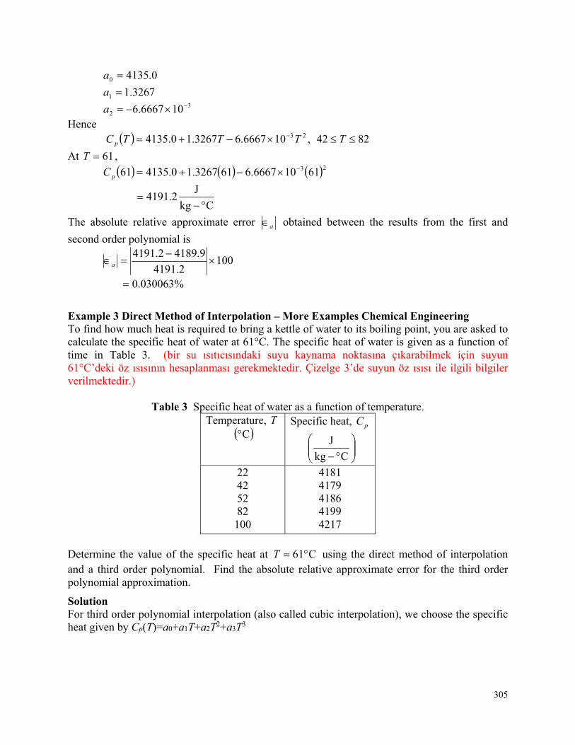
305

0.41350 a

3267.11 a

32 106667.6 a

Hence 8242,106667.63267.10.4135 23 TTTTC p

At 61T ,

23 61106667.6613267.10.413561 pC

Ckg

J2.4191

The absolute relative approximate error a obtained between the results from the first and

second order polynomial is

1002.4191

9.41892.4191

a

%030063.0

Example 3 Direct Method of Interpolation – More Examples Chemical Engineering To find how much heat is required to bring a kettle of water to its boiling point, you are asked to calculate the specific heat of water at 61°C. The specific heat of water is given as a function of time in Table 3. (bir su ısıtıcısındaki suyu kaynama noktasına çıkarabilmek için suyun 61°C’deki öz ısısının hesaplanması gerekmektedir. Çizelge 3’de suyun öz ısısı ile ilgili bilgiler verilmektedir.)

Table 3 Specific heat of water as a function of temperature. Temperature, T

C Specific heat, pC

Ckg

J

22 42 52 82 100

4181 4179 4186 4199 4217

Determine the value of the specific heat at C61T using the direct method of interpolation and a third order polynomial. Find the absolute relative approximate error for the third order polynomial approximation.

Solution For third order polynomial interpolation (also called cubic interpolation), we choose the specific heat given by Cp(T)=a0+a1T+a2T2+a3T3

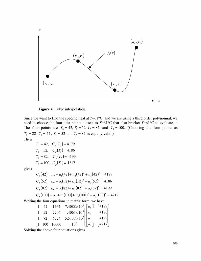
306

Figure 4 Cubic interpolation.

Since we want to find the specific heat at T=61°C, and we are using a third order polynomial, we need to choose the four data points closest to T=61°C that also bracket T=61°C to evaluate it. The four points are 82,52,42 210 TTT and .1003 T (Choosing the four points as

220 T , 421 T , 522 T and 823 T is equally valid.)

Then 4179 ,42 00 TCT p

4186 ,52 11 TCT p

4199 ,82 22 TCT p

4217,100 33 TCT p

gives

417942424242 33

2210 aaaaC p

418652525252 33

2210 aaaaC p

419982828282 33

2210 aaaaC p

4217100100100100 33

2210 aaaaC p

Writing the four equations in matrix form, we have

4217

4199

4186

4179

10100001001

105137.56724821

104061.12704521

104088.71764421

3

2

1

0

6

5

5

4

a

a

a

a

Solving the above four equations gives

y

00 , yx

11, yx xf3

22 , yx

33 , yx

x

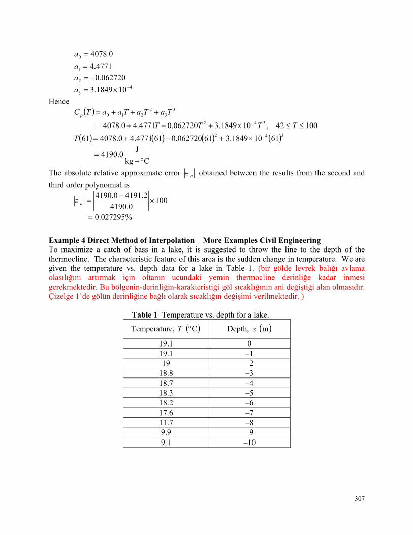
307

0.40780 a

4771.41 a

062720.02 a

43 101849.3 a

Hence 3

32

210 TaTaTaaTC p

10042,101849.3062720.04771.40.4078 342 TTTT

342 61101849.361062720.0614771.40.407861 T

Ckg

J0.4190

The absolute relative approximate error a obtained between the results from the second and

third order polynomial is

1000.4190

2.41910.4190

a

%027295.0

Example 4 Direct Method of Interpolation – More Examples Civil Engineering To maximize a catch of bass in a lake, it is suggested to throw the line to the depth of the thermocline. The characteristic feature of this area is the sudden change in temperature. We are given the temperature vs. depth data for a lake in Table 1. (bir gölde levrek balığı avlama olasılığını artırmak için oltanın ucundaki yemin thermocline derinliğe kadar inmesi gerekmektedir. Bu bölgenin-derinliğin-karakteristiği göl sıcaklığının ani değiştiği alan olmasıdır. Çizelge 1’de gölün derinliğine bağlı olarak sıcaklığın değişimi verilmektedir. ) Table 1 Temperature vs. depth for a lake.

Temperature, C T Depth, m z

19.1 0 19.1 –1 19 –2

18.8 –3 18.7 –4 18.3 –5 18.2 –6 17.6 –7 11.7 –8 9.9 –9 9.1 –10

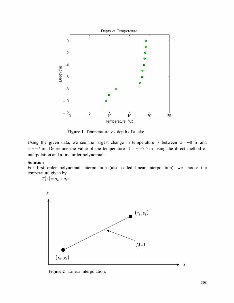
308

Figure 1 Temperature vs. depth of a lake. Using the given data, we see the largest change in temperature is between m8z and

m7z . Determine the value of the temperature at m5.7z using the direct method of interpolation and a first order polynomial.

Solution For first order polynomial interpolation (also called linear interpolation), we choose the temperature given by zaazT 10

Figure 2 Linear interpolation.

00, yx

11, yx

xf1

x

y

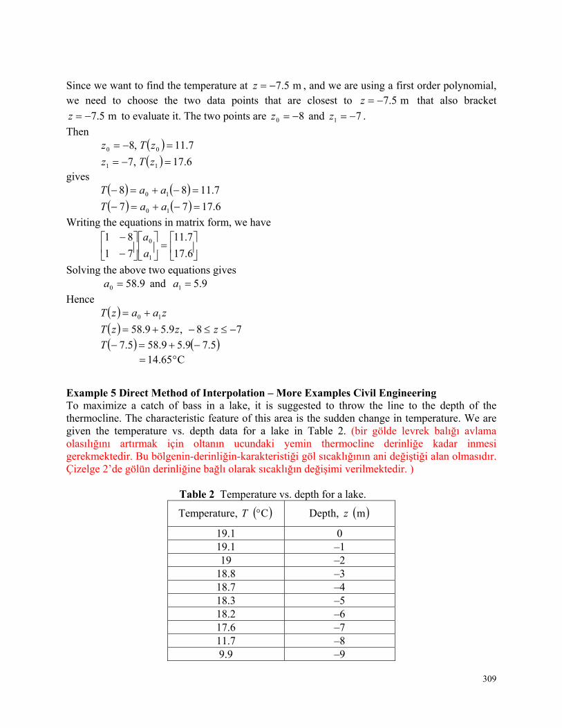
309

Since we want to find the temperature at m5.7z , and we are using a first order polynomial, we need to choose the two data points that are closest to m5.7z that also bracket

m5.7z to evaluate it. The two points are 80 z and 71 z .

Then 7.11,8 00 zTz

6.17,7 11 zTz gives 7.1188 10 aaT

6.1777 10 aaT

Writing the equations in matrix form, we have

6.17

7.11

71

81

1

0

a

a

Solving the above two equations gives 9.580 a and 9.51 a

Hence zaazT 10

78,9.59.58 zzzT

5.79.59.585.7 T C65.14

Example 5 Direct Method of Interpolation – More Examples Civil Engineering To maximize a catch of bass in a lake, it is suggested to throw the line to the depth of the thermocline. The characteristic feature of this area is the sudden change in temperature. We are given the temperature vs. depth data for a lake in Table 2. (bir gölde levrek balığı avlama olasılığını artırmak için oltanın ucundaki yemin thermocline derinliğe kadar inmesi gerekmektedir. Bu bölgenin-derinliğin-karakteristiği göl sıcaklığının ani değiştiği alan olmasıdır. Çizelge 2’de gölün derinliğine bağlı olarak sıcaklığın değişimi verilmektedir. ) Table 2 Temperature vs. depth for a lake.

Temperature, C T Depth, m z

19.1 0 19.1 –1 19 –2

18.8 –3 18.7 –4 18.3 –5 18.2 –6 17.6 –7 11.7 –8 9.9 –9

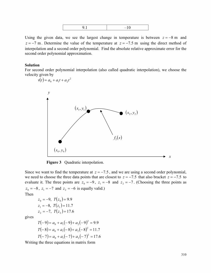
310

9.1 –10 Using the given data, we see the largest change in temperature is between m8z and

m7z . Determine the value of the temperature at m5.7z using the direct method of interpolation and a second order polynomial. Find the absolute relative approximate error for the second order polynomial approximation.

Solution For second order polynomial interpolation (also called quadratic interpolation), we choose the velocity given by

2210 tataatv

Figure 3 Quadratic interpolation.

Since we want to find the temperature at 5.7z , and we are using a second order polynomial, we need to choose the three data points that are closest to 5.7z that also bracket 5.7z to evaluate it. The three points are 90 z , 81 z and 72 z . (Choosing the three points as

80 z , 71 z and 62 z is equally valid.)

Then 9.9,9 00 zTz

7.11,8 11 zTz

6.17,7 22 zTz gives

9.9999 2210 aaaT

7.11888 2210 aaaT

6.17777 2210 aaaT

Writing the three equations in matrix form

00 , yx

11, yx 22 , yx

xf2

y

x

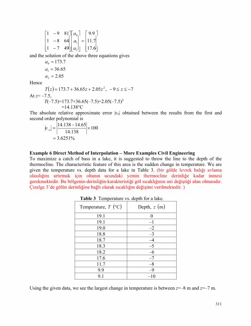
311

6.17

7.11

9.9

4971

6481

8191

2

1

0

a

a

a

and the solution of the above three equations gives 7.1730 a

65.361 a

05.22 a Hence 79,05.265.367.173 2 zzzzT At z= –7.5,

T(–7.5)=173.7+36.65(–7.5)+2.05(–7.5)2 =14.138°C The absolute relative approximate error |єa| obtained between the results from the first and second order polynomial is

100138.14

65.14138.14

a

%6251.3

Example 6 Direct Method of Interpolation – More Examples Civil Engineering To maximize a catch of bass in a lake, it is suggested to throw the line to the depth of the thermocline. The characteristic feature of this area is the sudden change in temperature. We are given the temperature vs. depth data for a lake in Table 3. (bir gölde levrek balığı avlama olasılığını artırmak için oltanın ucundaki yemin thermocline derinliğe kadar inmesi gerekmektedir. Bu bölgenin-derinliğin-karakteristiği göl sıcaklığının ani değiştiği alan olmasıdır. Çizelge 3’de gölün derinliğine bağlı olarak sıcaklığın değişimi verilmektedir. ) Table 3 Temperature vs. depth for a lake.

Temperature, C T Depth, m z

19.1 0 19.1 –1 19.0 –2 18.8 –3 18.7 –4 18.3 –5 18.2 –6 17.6 –7 11.7 –8 9.9 –9 9.1 –10

Using the given data, we see the largest change in temperature is between z=–8 m and z=–7 m.

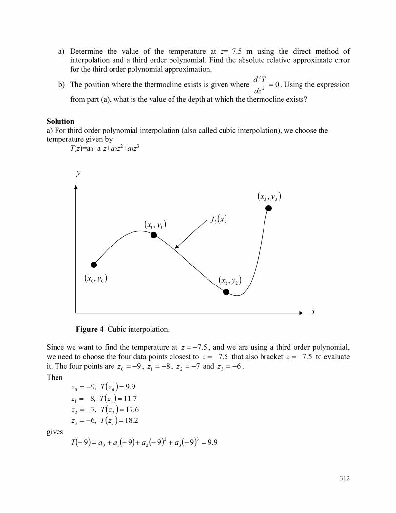
312

a) Determine the value of the temperature at z=–7.5 m using the direct method of interpolation and a third order polynomial. Find the absolute relative approximate error for the third order polynomial approximation.

b) The position where the thermocline exists is given where 02

2

dz

Td. Using the expression

from part (a), what is the value of the depth at which the thermocline exists?

Solution a) For third order polynomial interpolation (also called cubic interpolation), we choose the temperature given by T(z)=a0+a1z+a2z2+a3z3

Figure 4 Cubic interpolation.

Since we want to find the temperature at 5.7z , and we are using a third order polynomial, we need to choose the four data points closest to 5.7z that also bracket 5.7z to evaluate it. The four points are 90 z , 81 z , 72 z and 63 z .

Then 9.9,9 00 zTz

7.11,8 11 zTz

6.17,7 22 zTz

2.18,6 33 zTz

gives

9.99999 33

2210 aaaaT

y

00 , yx

11, yx xf3

22 , yx

33 , yx

x

313

7.118888 33

2210 aaaaT

6.177777 33

2210 aaaaT

2.186666 33

2210 aaaaT

Writing the four equations in matrix form, we have

2.18

6.17

7.11

9.9

2163661

3434971

5126481

7298191

3

2

1

0

a

a

a

a

Solving the above four equations gives 9.6150 a

58.2621 a

55.352 a

5667.13 a

Hence 3

32

210 zazazaazT

69,5667.155.3558.2629.615 32 zzzz

32 5.75667.15.755.355.758.2629.6155.7 T C725.14

The absolute relative approximate error a obtained between the results from the second and

third order polynomial is

100725.14

138.14725.14

a

%9898.3 b) To find the position of the thermocline, we must find the points of inflection of the third order

polynomial, given by 02

2

dz

Td

69,5667.155.3558.2629.615)( 32 zzzzzT

69,7.410.7158.262 2 zzzdz

dT

69,4.91.712

2

zzdz

Td

Simply setting this expression equal to zero, we get 0= –71.10–9.4z z=–7.5638 m

This answer can be verified due to the fact that it falls within the specified range of the third order polynomial and it also falls within the region of the greatest temperature change in the collected data from the lake.

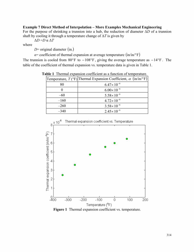
314

Example 7 Direct Method of Interpolation – More Examples Mechanical Engineering For the purpose of shrinking a trunnion into a hub, the reduction of diameter ΔD of a trunnion shaft by cooling it through a temperature change of ΔT is given by ΔD =D α ΔT where D= original diameter in.

α= coefficient of thermal expansion at average temperature Fin/in/ The trunnion is cooled from F80 to F108 , giving the average temperature as F14 . The table of the coefficient of thermal expansion vs. temperature data is given in Table 1. Table 1 Thermal expansion coefficient as a function of temperature.

Temperature, T (°F) Thermal Expansion Coefficient, Fin/in/

80 6.47 610 0 6.00 610

–60 5.58 610 –160 4.72 610 –260 3.58 610 –340 2.45 610

Figure 1 Thermal expansion coefficient vs. temperature.

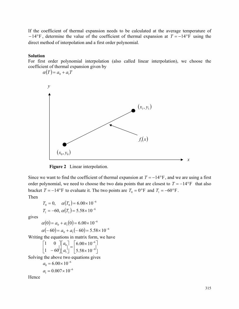
315

If the coefficient of thermal expansion needs to be calculated at the average temperature of F14 , determine the value of the coefficient of thermal expansion at F14T using the

direct method of interpolation and a first order polynomial.

Solution For first order polynomial interpolation (also called linear interpolation), we choose the coefficient of thermal expansion given by TaaT 10

Figure 2 Linear interpolation.

Since we want to find the coefficient of thermal expansion at F14T , and we are using a first order polynomial, we need to choose the two data points that are closest to F14T that also

bracket F14T to evaluate it. The two points are F00 T and F601 T .

Then 6

00 1000.6 ,0 TT

611 1058.5,60 TT

gives

610 1000.600 aa

610 1058.56060 aa

Writing the equations in matrix form, we have

6

6

1

0

10 58.5

10 00.6

601

01

a

a

Solving the above two equations gives 6

0 1000.6 a

61 10007.0 a

Hence

00, yx

11, yx

xf1

x

y

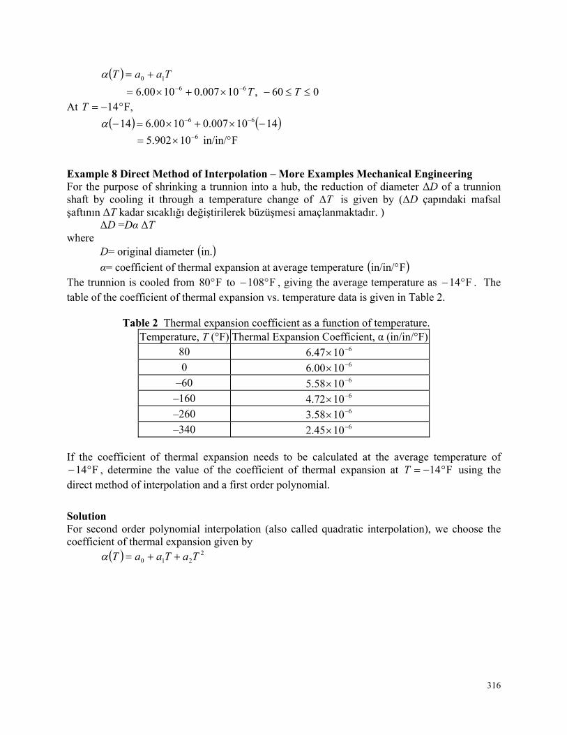
316

TaaT 10 060,10 007.01000.6 66 TT At F,14T

1410 007.010 00.614 66

Fin/in/10902.5 6

Example 8 Direct Method of Interpolation – More Examples Mechanical Engineering For the purpose of shrinking a trunnion into a hub, the reduction of diameter ΔD of a trunnion shaft by cooling it through a temperature change of T is given by (ΔD çapındaki mafsal şaftının ΔT kadar sıcaklığı değiştirilerek büzüşmesi amaçlanmaktadır. ) ΔD =Dα ΔT where D= original diameter in.

α= coefficient of thermal expansion at average temperature Fin/in/ The trunnion is cooled from F80 to F108 , giving the average temperature as F14 . The table of the coefficient of thermal expansion vs. temperature data is given in Table 2. Table 2 Thermal expansion coefficient as a function of temperature.

Temperature, T (°F) Thermal Expansion Coefficient, α (in/in/°F) 80 6.47 610 0 6.00 610

–60 5.58 610 –160 4.72 610 –260 3.58 610 –340 2.45 610

If the coefficient of thermal expansion needs to be calculated at the average temperature of

F14 , determine the value of the coefficient of thermal expansion at F14T using the direct method of interpolation and a first order polynomial.

Solution For second order polynomial interpolation (also called quadratic interpolation), we choose the coefficient of thermal expansion given by 2

210 TaTaaT

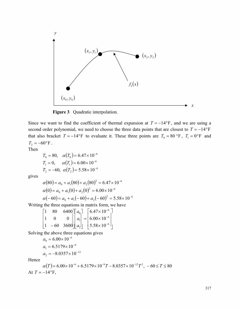
317

Figure 3 Quadratic interpolation.

Since we want to find the coefficient of thermal expansion at F14T , and we are using a second order polynomial, we need to choose the three data points that are closest to F14T

that also bracket F14T to evaluate it. These three points are F800 T , F01 T and

F602 T . Then 6

00 1047.6 ,80 TT

611 1000.6 ,0 TT

622 1058.5,60 TT

gives

62210 1047.6808080 aaa

62210 1000.6000 aaa

62210 1058.5606060 aaa

Writing the three equations in matrix form, we have

10 58.5

10 00.6

10 47.6

3600601

001

6400801

6

6

6

2

1

0

a

a

a

Solving the above three equations gives

6

0 1000.6 a

9

1 105179.6 a

12

2 100357.8 a Hence 8060,100357.8105179.610 00.6 21296 TTTT At F,14T

00 , yx

11, yx 22 , yx

xf2

y

x

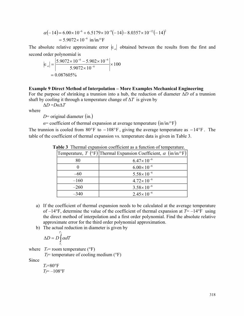
318

21296 14100357.814105179.610 00.614

Fin/in/109072.5 6

The absolute relative approximate error a obtained between the results from the first and

second order polynomial is

100

109072.5

10902.5109072.56

66

a

%087605.0

Example 9 Direct Method of Interpolation – More Examples Mechanical Engineering For the purpose of shrinking a trunnion into a hub, the reduction of diameter ΔD of a trunnion shaft by cooling it through a temperature change of ΔT is given by ΔD =DαΔT where D= original diameter in.

α= coefficient of thermal expansion at average temperature Fin/in/ The trunnion is cooled from F80 to F108 , giving the average temperature as F14 . The table of the coefficient of thermal expansion vs. temperature data is given in Table 3. Table 3 Thermal expansion coefficient as a function of temperature.

Temperature, F T Thermal Expansion Coefficient, Fin/in/

80 6.47 610 0 6.00 610

–60 5.58 610 –160 4.72 610 –260 3.58 610 –340 2.45 610

a) If the coefficient of thermal expansion needs to be calculated at the average temperature

of –14°F, determine the value of the coefficient of thermal expansion at T= –14°F using the direct method of interpolation and a first order polynomial. Find the absolute relative approximate error for the third order polynomial approximation.

b) The actual reduction in diameter is given by

f

r

T

T

dTDD

where Tr= room temperature (°F) Tf= temperature of cooling medium (°F) Since Tr=80°F Tf= –108°F

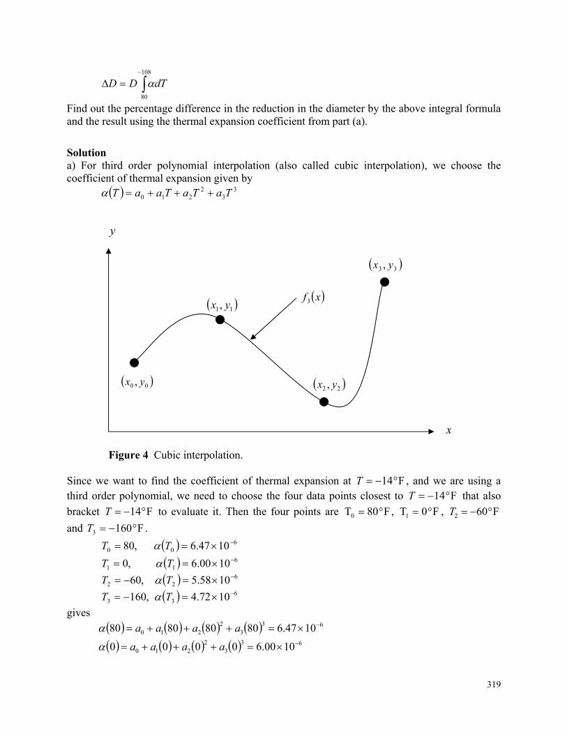
319

108

80

dTDD

Find out the percentage difference in the reduction in the diameter by the above integral formula and the result using the thermal expansion coefficient from part (a).

Solution a) For third order polynomial interpolation (also called cubic interpolation), we choose the coefficient of thermal expansion given by 3

32

210 TaTaTaaT

Figure 4 Cubic interpolation.

Since we want to find the coefficient of thermal expansion at F14T , and we are using a third order polynomial, we need to choose the four data points closest to F14T that also

bracket F14T to evaluate it. Then the four points are F80T0 , F0T1 , F602 T

and F1603 T .

600 1047.6 ,80 TT

611 1000.6 ,0 TT

622 1058.5 ,60 TT

633 1072.4,160 TT

gives

633

2210 10 47.680808080 aaaa

633

2210 10 00.60000 aaaa

y

00 , yx

11, yx xf3

22 , yx

33 , yx

x

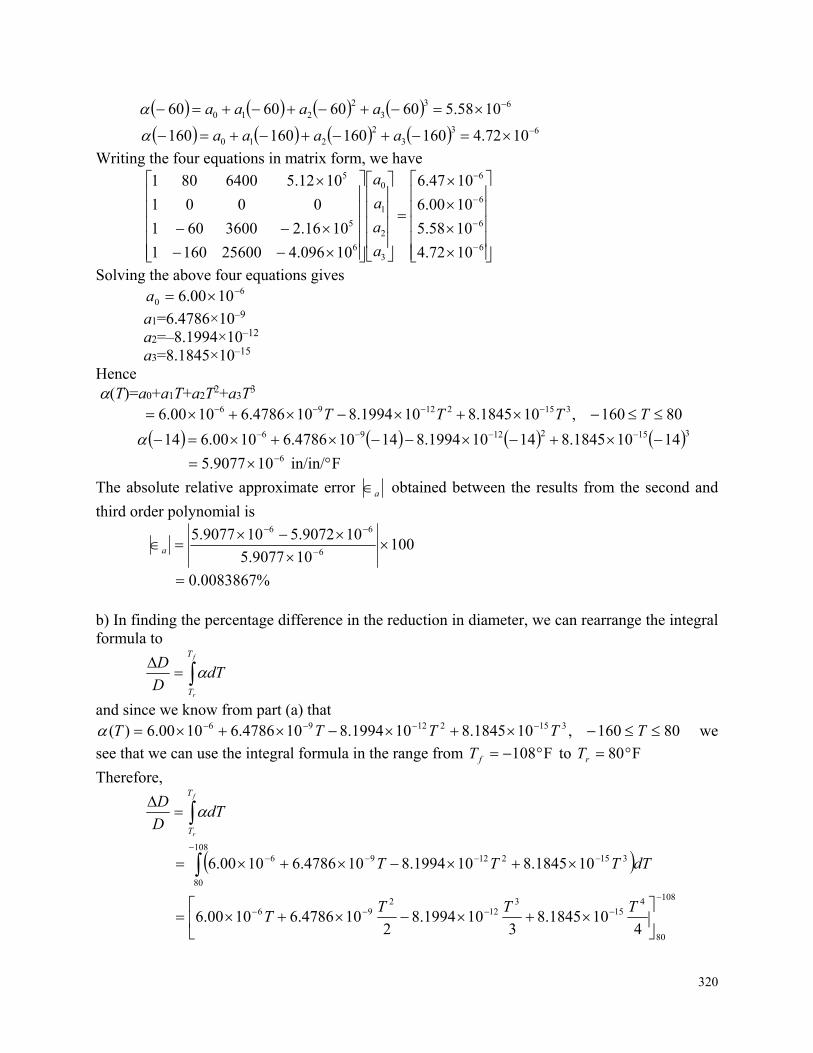
320

633

2210 10 58.560606060 aaaa

633

2210 10 72.4160160160160 aaaa

Writing the four equations in matrix form, we have

6

6

6

6

3

2

1

0

6

5

5

10 72.4

10 58.5

10 00.6

10 47.6

10096.4256001601

1016.23600601

0001

1012.56400801

a

a

a

a

Solving the above four equations gives

6

0 1000.6 a a1=6.4786×10–9 a2=–8.1994×10–12 a3=8.1845×10–15 Hence (T)=a0+a1T+a2T2+a3T3 80160,101845.8101994.8104786.610 00.6 31521296 TTTT

31521296 14101845.814101994.814104786.61000.614

Fin/in/109077.5 6

The absolute relative approximate error a obtained between the results from the second and

third order polynomial is

100109077.5

109072.5109077.56

66

a

%0083867.0 b) In finding the percentage difference in the reduction in diameter, we can rearrange the integral formula to

f

r

T

T

dTD

D

and since we know from part (a) that 80160,101845.8101994.8104786.61000.6)( 31521296 TTTTT we

see that we can use the integral formula in the range from F108fT to F80rT

Therefore,

f

r

T

T

dTD

D

108

80

31521296 101845.8101994.8104786.610 00.6 dTTTT

108

80

415

312

296

4101845.8

3101994.8

2104786.61000.6

TTTT

321

6109.1105

So in/in109.1105 6D

D using the actual reduction in diameter integral formula. If we use

the average value for the coefficient of thermal expansion from part (a), we get

TD

D

rf TT

80108109077.5 6

6106.1110

and in/in106.1110 6D

D using the average value of the coefficient of thermal expansion

using a third order polynomial. Considering the integral to be the more accurate calculation, the percentage difference would be

100109.1105

106.1110109.11056

66

a

%42775.0

INTERPOLATION Topic Direct Method of Interpolation Summary Examples of direct method of interpolation. Major Chemical Engineering Authors Autar Kaw Date Aralık 8, 2016 Web Site http://numericalmethods.eng.usf.edu