Introduction to Nevanlinna theoryminru/talk1.pdfIntroduction: The algebraic case I The well-known fundamental theorem of algebra states that, for every complex polynomial P, deg P

Introduction to Nevanlinna theory

Min Ru

University of Houston

[email protected]

1 / 1

Introduction: The algebraic case

I The well-known fundamental theorem of algebra statesthat, for every complex polynomial P,

deg P = #(P = 0).

I For any rational function f on a compact Riemann surface S ,we also have deg f = #(f = 0) = #(f =∞).

I Regarding f as mapping f : S → C ∪ {∞}, and leta1, . . . , aq ∈ C ∪ {∞}. Let E = f −1({a1, . . . , aq}) ⊂ S .Define the ramification r(E ) :=

∑p∈E (υ(p)− 1), here, for

f : S → S ′, let z ,w be a local coordinates for S and S ′ at pand f (p) respectively, such that w = zυ(p).

I Since, for 1 ≤ j ≤ q, d =∑

p∈f −1(aj )υ(p), qd = |E |+ r(E ).

I Riemann-Hurwitz: Let f : S → S ′. Then(2g − 2) = deg(f )(2g ′ − 2) +

∑p∈S(υ(p)− 1).The proof

comes from (f ∗ω) = f ∗(ω) +∑

p∈S(υ(p)− 1)p and then useRR (or Gauss-Bonnet) deg KS = 2g − 2.

2 / 1

Introduction: The algebraic caseI The well-known fundamental theorem of algebra states

that, for every complex polynomial P,

deg P = #(P = 0).






p∈f −1(aj )υ(p), qd = |E |+ r(E ).





2 / 1



deg P = #(P = 0).






p∈f −1(aj )υ(p), qd = |E |+ r(E ).





2 / 1



deg P = #(P = 0).



∑p∈E (υ(p)− 1),

here, forf : S → S ′, let z ,w be a local coordinates for S and S ′ at pand f (p) respectively, such that w = zυ(p).


p∈f −1(aj )υ(p), qd = |E |+ r(E ).





2 / 1



deg P = #(P = 0).






p∈f −1(aj )υ(p), qd = |E |+ r(E ).





2 / 1



deg P = #(P = 0).






p∈f −1(aj )υ(p), qd = |E |+ r(E ).





2 / 1



deg P = #(P = 0).






p∈f −1(aj )υ(p), qd = |E |+ r(E ).


∑p∈S(υ(p)− 1).

The proofcomes from (f ∗ω) = f ∗(ω) +

∑p∈S(υ(p)− 1)p and then use

RR (or Gauss-Bonnet) deg KS = 2g − 2.

2 / 1



deg P = #(P = 0).






p∈f −1(aj )υ(p), qd = |E |+ r(E ).





2 / 1

I Applying Riemann-Hurwitz, we haver(E ) ≤ 2 deg(f ) + 2(g − 1), where g =genus of S , so we get

I SMT: f : S → C ∪ {∞}, and let a1, . . . , aq ∈ C ∪ {∞}. LetE = f −1({a1, . . . , aq}) ⊂ S . Then

(q − 2) deg(f ) ≤ |E |+ 2(g − 1).

I ABC Theorem: k=algebraically closed field, C/k= smoothprojective curve of genus g . Let a, b ∈ k(C ) be non-constantsuch that a + b = 1. Then deg(a) = deg(b) ≤ |E |+ 2(g − 1)where E is the set of zeros and poles of a, b.

3 / 1



(q − 2) deg(f ) ≤ |E |+ 2(g − 1).


3 / 1



(q − 2) deg(f ) ≤ |E |+ 2(g − 1).


3 / 1

I The theory of algebraic curves in the projective spaces:

Letf : S → Pn(C) be a linearly nondegenerate algebraic curveand let f(z) = (f0(z), ..., fn(z)) be a reduced representation.

I We define the i th associate curve f i : S → P(∧i+1Cn+1) byf i (z) = P(f i (z)) where f i (z) = f(z) ∧ f ′(z) ∧ · · · ∧ f(i)(z).

I β(z0), the ramification index of f at z0, isβ(z0) := min0≤i≤n{ordz0(∂fi/∂z)}. Write f(z) =(1+ · · · , z1+α1 + · · · , z2+α1+α2 + · · · , · · · , zn+α1+···+αn + · · · ),Then βi (z0) = αi+1. Let βi =

∑p∈S βi (p).

I Plucker formula:di−1 − 2di + di+1 = 2g − 2− βi , 1 ≤ i ≤ n − 1, wheredi = deg(f i ).

4 / 1

I The theory of algebraic curves in the projective spaces: Letf : S → Pn(C) be a linearly nondegenerate algebraic curveand let f(z) = (f0(z), ..., fn(z)) be a reduced representation.



∑p∈S βi (p).


4 / 1




∑p∈S βi (p).


4 / 1



I β(z0), the ramification index of f at z0, isβ(z0) := min0≤i≤n{ordz0(∂fi/∂z)}.

Write f(z) =(1+ · · · , z1+α1 + · · · , z2+α1+α2 + · · · , · · · , zn+α1+···+αn + · · · ),Then βi (z0) = αi+1. Let βi =

∑p∈S βi (p).


4 / 1



I β(z0), the ramification index of f at z0, isβ(z0) := min0≤i≤n{ordz0(∂fi/∂z)}. Write f(z) =(1+ · · · , z1+α1 + · · · , z2+α1+α2 + · · · , · · · , zn+α1+···+αn + · · · ),Then βi (z0) = αi+1.

Let βi =∑

p∈S βi (p).


4 / 1




∑p∈S βi (p).


4 / 1




∑p∈S βi (p).


4 / 1

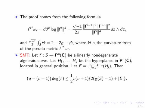
I The proof comes from the following formula

f i ∗ωi = ddc log ‖f i‖2 =

√−1

2π

‖f i−1‖2‖f i+1‖2

‖f i‖4dz ∧ dz̄ ,

and√−12

∫S Θ = 2− 2g − βi , where Θ is the curvature from

of the pseudo-metric f i ∗ωi .

I SMT: Let f : S → Pn(C) be a linearly nondegeneratealgebraic curve. Let H1, . . . ,Hq be the hyperplanes in Pn(C),located in general position. Let E = ∪q

j=1f−1(Hj). Then

(q − (n + 1)) deg(f ) ≤ 1

2n(n + 1){2(g(S)− 1) + |E |}.

5 / 1



√−1

2π

‖f i−1‖2‖f i+1‖2

‖f i‖4dz ∧ dz̄ ,

and√−12




j=1f−1(Hj). Then

(q − (n + 1)) deg(f ) ≤ 1

2n(n + 1){2(g(S)− 1) + |E |}.

5 / 1



√−1

2π

‖f i−1‖2‖f i+1‖2

‖f i‖4dz ∧ dz̄ ,

and√−12




j=1f−1(Hj). Then

(q − (n + 1)) deg(f ) ≤ 1

2n(n + 1){2(g(S)− 1) + |E |}.

5 / 1

Nevanlinna Theory

I Nevanlinna theory studies holomorphic curves f : C→ Pn, ormore generally, meromorphic mappings f : A→ M, whereA,M be smooth algebraic varieties with M projective.

I To do so, we simply restrict f to the disc 4(r) or A(r) for rsufficiently large.

I The most important case is when A is affine (parabolic type),i.e. There is an exhaustion function on A with dim A = m,τ : A→ R ∪ {∞} such that τ is proper, ddcτ ≥ 0 and(ddcτ)m−1 6≡ 0 but (ddcτ)m ≡ 0. An example isA = Cm, τ = log‖z‖ (can be outside a compact set). Forsimplicity, we only consider A = Cm.

I Then the mapping f is generally not an algebraic mapping.

6 / 1

Nevanlinna Theory





6 / 1

Nevanlinna Theory





6 / 1

Nevanlinna Theory



I The most important case is when A is affine (parabolic type),i.e. There is an exhaustion function on A with dim A = m,τ : A→ R ∪ {∞} such that τ is proper, ddcτ ≥ 0 and(ddcτ)m−1 6≡ 0 but (ddcτ)m ≡ 0.

An example isA = Cm, τ = log‖z‖ (can be outside a compact set). Forsimplicity, we only consider A = Cm.


6 / 1

Nevanlinna Theory



I The most important case is when A is affine (parabolic type),i.e. There is an exhaustion function on A with dim A = m,τ : A→ R ∪ {∞} such that τ is proper, ddcτ ≥ 0 and(ddcτ)m−1 6≡ 0 but (ddcτ)m ≡ 0. An example isA = Cm, τ = log‖z‖ (can be outside a compact set).

Forsimplicity, we only consider A = Cm.


6 / 1

Nevanlinna Theory





6 / 1

Nevanlinna Theory





6 / 1

Nevanlinna Theory





6 / 1

I Nevanlinna theory studies the position of f (A) relative to thealgebraic subvarieties of M.

There are two basic questions:

I (A) Find an upper bound on the size of Zf in terms of Z andgrowth of mapping f (The First Main Type Theorem).

I (B) Find a lower bound again on the size of Zf in terms of Zand growth of mapping f (The Second Main Type Theorem).

7 / 1

I Nevanlinna theory studies the position of f (A) relative to thealgebraic subvarieties of M. There are two basic questions:



7 / 1




7 / 1




7 / 1




7 / 1

I The ”associate curve f i (z) = P(f(z) ∧ f ′(z) ∧ · · · ∧ f(i)(z))method” was carried over to f : C→ Pn by Ahlfors to proveSMT for hyperplanes.

I The step of the Hurwitz’s theorem ”by considering f ∗ω” wasbasically replaced by the LDL in Nevanlinna’s proof of SMTfor mero functions: f meromorphic, then∫ 2π

0log+

∣∣∣∣ f ′f (re iθ)

∣∣∣∣ dθ2π≤exc O(log rTf (r)).

I H. Cartan also used the LDL to SMT for hyperplanes.

I Consider on P1 with inhomogeneous coordinate w , andconsider ω = dw/w (differential form with log-singularityalong D = {0,∞}), and write f ∗ω = ζdz , then∫ 2π

0 log+ |ζ(re iθ)|dθ2π ≤exc O(log rTf (r)).

8 / 1



0log+

∣∣∣∣ f ′f (re iθ)





8 / 1



0log+

∣∣∣∣ f ′f (re iθ)





8 / 1



0log+

∣∣∣∣ f ′f (re iθ)





8 / 1



0log+

∣∣∣∣ f ′f (re iθ)





8 / 1

I A k differential on a n-dim manifold X with local coordinatesz1, . . . , zn is locally a polynomial in dz l

j , 1 ≤ l ≤ k , 1 ≤ j ≤ n.

I Schwarz Lemma for jet differential: X=complex manifold,ω=holomorphic jet differential, vanishing on an ample divisor,then f ∗ω ≡ 0. (If ω has log-singularity along D, then weconsider f : C→ X − D).

I Reasons: (a) Can use meromorphic functions as coordinatefunctions to bound ω by logarithmic derivative of globalmeromorphic functions, so LDL can be applied. (b) Vanishingon an ample divisor E contributes to faster growth thanO(log Tf (r) + log r).

9 / 1


j , 1 ≤ l ≤ k , 1 ≤ j ≤ n.

I Schwarz Lemma for jet differential: X=complex manifold,ω=holomorphic jet differential, vanishing on an ample divisor,then f ∗ω ≡ 0.

(If ω has log-singularity along D, then weconsider f : C→ X − D).


9 / 1


j , 1 ≤ l ≤ k , 1 ≤ j ≤ n.



9 / 1


j , 1 ≤ l ≤ k , 1 ≤ j ≤ n.


I Reasons: (a) Can use meromorphic functions as coordinatefunctions to bound ω by logarithmic derivative of globalmeromorphic functions, so LDL can be applied.

(b) Vanishingon an ample divisor E contributes to faster growth thanO(log Tf (r) + log r).

9 / 1


j , 1 ≤ l ≤ k , 1 ≤ j ≤ n.



9 / 1

I Application to hyperbolicity problems (i.e. no non-constantholomorphic map from C to the manifold): Image of f , ask-jet, satisfy the differential equation ω = 0 on X .

I If there are enough such ω, then the system of all equationsω = 0 does not admit any local solution curve. Such X ishyperbolic.

I The construction (existence) of holomorphic jet differential onM can be achieved by using RR+vanishing theorem, or usingHolomorphic Morse inequalities.

10 / 1




10 / 1




10 / 1




10 / 1

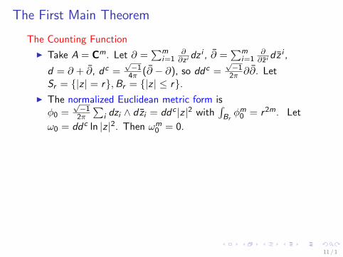
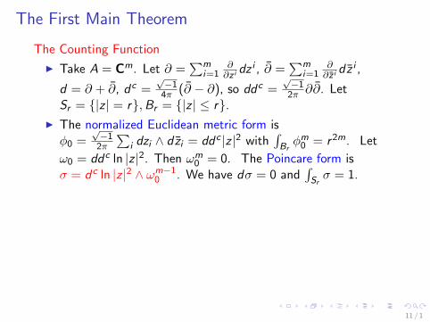
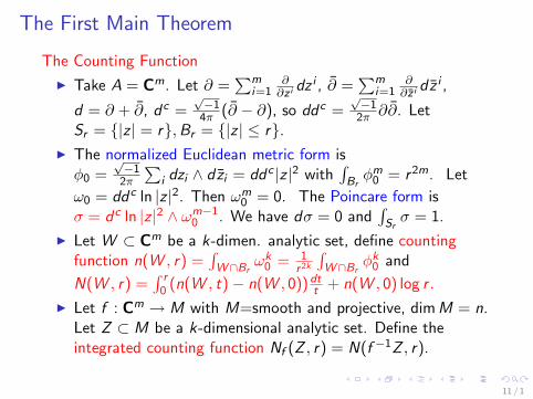
The First Main Theorem

The Counting Function

I Take A = Cm. Let ∂ =∑m

i=1∂∂z i dz i , ∂̄ =

∑mi=1

∂∂z̄ i dz̄ i ,

d = ∂ + ∂̄, dc =√−1

4π (∂̄ − ∂), so ddc =√−1

2π ∂∂̄. LetSr = {|z | = r},Br = {|z | ≤ r}.

I The normalized Euclidean metric form isφ0 =

√−1

2π

∑i dzi ∧ dz̄i = ddc |z |2 with

∫Brφm

0 = r2m. Let

ω0 = ddc ln |z |2. Then ωm0 = 0. The Poincare form is

σ = dc ln |z |2 ∧ ωm−10 . We have dσ = 0 and

∫Srσ = 1.

I Let W ⊂ Cm be a k-dimen. analytic set, define countingfunction n(W , r) =

∫W∩Br

ωk0 = 1

r2k

∫W∩Br

φk0 and

N(W , r) =∫ r

0 (n(W , t)− n(W , 0))dtt + n(W , 0) log r .

I Let f : Cm → M with M=smooth and projective, dim M = n.Let Z ⊂ M be a k-dimensional analytic set. Define theintegrated counting function Nf (Z , r) = N(f −1Z , r).

11 / 1




i=1∂∂z i dz i , ∂̄ =

∑mi=1

∂∂z̄ i dz̄ i ,

d = ∂ + ∂̄, dc =√−1

4π (∂̄ − ∂), so ddc =√−1

2π ∂∂̄. LetSr = {|z | = r},Br = {|z | ≤ r}.


√−1

2π


∫Brφm

0 = r2m. Let



∫Srσ = 1.


∫W∩Br

ωk0 = 1

r2k

∫W∩Br

φk0 and

N(W , r) =∫ r

0 (n(W , t)− n(W , 0))dtt + n(W , 0) log r .


11 / 1




i=1∂∂z i dz i , ∂̄ =

∑mi=1

∂∂z̄ i dz̄ i ,

d = ∂ + ∂̄, dc =√−1

4π (∂̄ − ∂), so ddc =√−1

2π ∂∂̄.

LetSr = {|z | = r},Br = {|z | ≤ r}.


√−1

2π


∫Brφm

0 = r2m. Let



∫Srσ = 1.


∫W∩Br

ωk0 = 1

r2k

∫W∩Br

φk0 and

N(W , r) =∫ r

0 (n(W , t)− n(W , 0))dtt + n(W , 0) log r .


11 / 1




i=1∂∂z i dz i , ∂̄ =

∑mi=1

∂∂z̄ i dz̄ i ,

d = ∂ + ∂̄, dc =√−1

4π (∂̄ − ∂), so ddc =√−1

2π ∂∂̄. LetSr = {|z | = r},Br = {|z | ≤ r}.


√−1

2π


∫Brφm

0 = r2m. Let



∫Srσ = 1.


∫W∩Br

ωk0 = 1

r2k

∫W∩Br

φk0 and

N(W , r) =∫ r

0 (n(W , t)− n(W , 0))dtt + n(W , 0) log r .


11 / 1




i=1∂∂z i dz i , ∂̄ =

∑mi=1

∂∂z̄ i dz̄ i ,

d = ∂ + ∂̄, dc =√−1

4π (∂̄ − ∂), so ddc =√−1

2π ∂∂̄. LetSr = {|z | = r},Br = {|z | ≤ r}.


√−1

2π


∫Brφm

0 = r2m.

Let



∫Srσ = 1.


∫W∩Br

ωk0 = 1

r2k

∫W∩Br

φk0 and

N(W , r) =∫ r

0 (n(W , t)− n(W , 0))dtt + n(W , 0) log r .


11 / 1




i=1∂∂z i dz i , ∂̄ =

∑mi=1

∂∂z̄ i dz̄ i ,

d = ∂ + ∂̄, dc =√−1

4π (∂̄ − ∂), so ddc =√−1

2π ∂∂̄. LetSr = {|z | = r},Br = {|z | ≤ r}.


√−1

2π


∫Brφm

0 = r2m. Let

ω0 = ddc ln |z |2. Then ωm0 = 0.

The Poincare form isσ = dc ln |z |2 ∧ ωm−1

0 . We have dσ = 0 and∫Srσ = 1.


∫W∩Br

ωk0 = 1

r2k

∫W∩Br

φk0 and

N(W , r) =∫ r

0 (n(W , t)− n(W , 0))dtt + n(W , 0) log r .


11 / 1




i=1∂∂z i dz i , ∂̄ =

∑mi=1

∂∂z̄ i dz̄ i ,

d = ∂ + ∂̄, dc =√−1

4π (∂̄ − ∂), so ddc =√−1

2π ∂∂̄. LetSr = {|z | = r},Br = {|z | ≤ r}.


√−1

2π


∫Brφm

0 = r2m. Let



∫Srσ = 1.


∫W∩Br

ωk0 = 1

r2k

∫W∩Br

φk0 and

N(W , r) =∫ r

0 (n(W , t)− n(W , 0))dtt + n(W , 0) log r .


11 / 1




i=1∂∂z i dz i , ∂̄ =

∑mi=1

∂∂z̄ i dz̄ i ,

d = ∂ + ∂̄, dc =√−1

4π (∂̄ − ∂), so ddc =√−1

2π ∂∂̄. LetSr = {|z | = r},Br = {|z | ≤ r}.


√−1

2π


∫Brφm

0 = r2m. Let



∫Srσ = 1.


∫W∩Br

ωk0 = 1

r2k

∫W∩Br

φk0 and

N(W , r) =∫ r

0 (n(W , t)− n(W , 0))dtt + n(W , 0) log r .


11 / 1




i=1∂∂z i dz i , ∂̄ =

∑mi=1

∂∂z̄ i dz̄ i ,

d = ∂ + ∂̄, dc =√−1

4π (∂̄ − ∂), so ddc =√−1

2π ∂∂̄. LetSr = {|z | = r},Br = {|z | ≤ r}.


√−1

2π


∫Brφm

0 = r2m. Let



∫Srσ = 1.


∫W∩Br

ωk0 = 1

r2k

∫W∩Br

φk0 and

N(W , r) =∫ r

0 (n(W , t)− n(W , 0))dtt + n(W , 0) log r .

I Let f : Cm → M with M=smooth and projective, dim M = n.

Let Z ⊂ M be a k-dimensional analytic set. Define theintegrated counting function Nf (Z , r) = N(f −1Z , r).

11 / 1




i=1∂∂z i dz i , ∂̄ =

∑mi=1

∂∂z̄ i dz̄ i ,

d = ∂ + ∂̄, dc =√−1

4π (∂̄ − ∂), so ddc =√−1

2π ∂∂̄. LetSr = {|z | = r},Br = {|z | ≤ r}.


√−1

2π


∫Brφm

0 = r2m. Let



∫Srσ = 1.


∫W∩Br

ωk0 = 1

r2k

∫W∩Br

φk0 and

N(W , r) =∫ r

0 (n(W , t)− n(W , 0))dtt + n(W , 0) log r .


11 / 1

Nevanlinna’s Growth Functions

I Let f : Cm → M, and let L→ M be a positive line bundlehaving a metric with h. Define, for 1 ≤ j ≤ m,

tj(r) =

∫Br

(f ∗c1(L, h))j ∧ ωm−j0 , Tj(r) =

∫ r

0tj(t)

dt

t

andTf (r) := T1(r).

12 / 1


I Let f : Cm → M, and let L→ M be a positive line bundlehaving a metric with h.

Define, for 1 ≤ j ≤ m,

tj(r) =

∫Br

(f ∗c1(L, h))j ∧ ωm−j0 , Tj(r) =

∫ r

0tj(t)

dt

t

andTf (r) := T1(r).

12 / 1


I Let f : Cm → M, and let L→ M be a positive line bundlehaving a metric with h. Define, for 1 ≤ j ≤ m,

tj(r) =

∫Br

(f ∗c1(L, h))j ∧ ωm−j0 , Tj(r) =

∫ r

0tj(t)

dt

t

andTf (r) := T1(r).

12 / 1

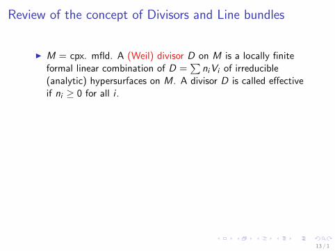
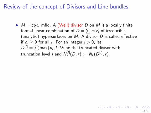
Review of the concept of Divisors and Line bundles

I M = cpx. mfld. A (Weil) divisor D on M is a locally finiteformal linear combination of D =

∑niVi of irreducible

(analytic) hypersurfaces on M. A divisor D is called effectiveif ni ≥ 0 for all i . For an integer l > 0, letD [l ] =

∑max{ni , l}Di be the truncated divisor with

truncation level l and N[l ]f (D, r) := Nf (D [l ], r).

I f =mero on M. Define (f ) =∑

ordV (f )V , where V ⊂ M isirred. analytic set. Note: Let h be a local defining function forV near p. For g holo. near p, order ordV ,p(g) of g along V=the largest positive integer k such that g/hk is holomorphicaround p. Note that ordV ,p(g) is indep. of p ∈ V . Thisextends to ordV (f ) for mero f .

13 / 1




(analytic) hypersurfaces on M.

A divisor D is called effectiveif ni ≥ 0 for all i . For an integer l > 0, letD [l ] =





13 / 1




(analytic) hypersurfaces on M. A divisor D is called effectiveif ni ≥ 0 for all i .

For an integer l > 0, letD [l ] =





13 / 1









13 / 1








ordV (f )V , where V ⊂ M isirred. analytic set.

Note: Let h be a local defining function forV near p. For g holo. near p, order ordV ,p(g) of g along V=the largest positive integer k such that g/hk is holomorphicaround p. Note that ordV ,p(g) is indep. of p ∈ V . Thisextends to ordV (f ) for mero f .

13 / 1








ordV (f )V , where V ⊂ M isirred. analytic set. Note: Let h be a local defining function forV near p. For g holo. near p, order ordV ,p(g) of g along V=the largest positive integer k such that g/hk is holomorphicaround p.

Note that ordV ,p(g) is indep. of p ∈ V . Thisextends to ordV (f ) for mero f .

13 / 1









13 / 1









13 / 1

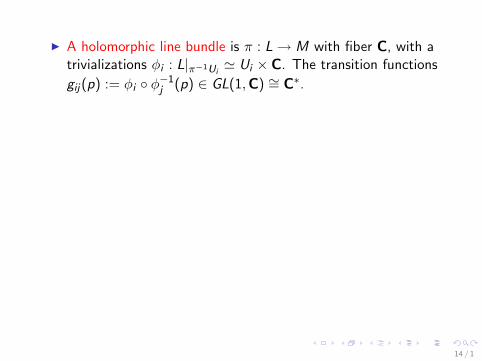
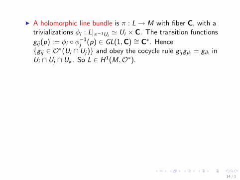
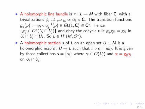
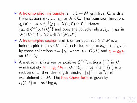
I A holomorphic line bundle is π : L→ M with fiber C, with atrivializations φi : L|π−1Ui

' Ui × C. The transition functions

gij(p) := φi ◦ φ−1j (p) ∈ GL(1,C) ∼= C∗.

Hence{gij ∈ O∗(Ui ∩ Uj)} and obey the cocycle rule gijgjk = gik inUi ∩ Uj ∩ Uk . So L ∈ H1(M,O∗).

I A holomorphic section s of L on an open set U ⊂ M is aholomorphic map s : U → L such that π ◦ s = idU . It is givenby those collections s = {si} where si ∈ O(Ui ) and si = gijsjon Ui ∩ Uj .

I A metric in L is given by positive C∞ functions {hi} in Ui

which satisfy hj = |gij |2hi in Ui ∩ Uj . Thus, if s = {si} is asection of L, then the length function ‖s‖2 = |si |2hi iswell-defined on M. The first Chern form is given byc1(L, h) = −ddc log hi .

14 / 1



gij(p) := φi ◦ φ−1j (p) ∈ GL(1,C) ∼= C∗. Hence

{gij ∈ O∗(Ui ∩ Uj)} and obey the cocycle rule gijgjk = gik inUi ∩ Uj ∩ Uk . So L ∈ H1(M,O∗).




14 / 1








14 / 1








14 / 1

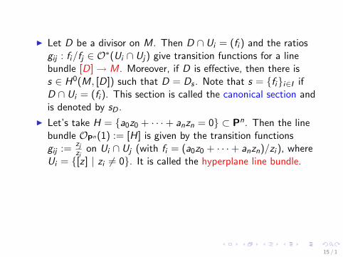
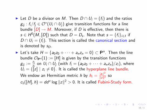
I Let D be a divisor on M. Then D ∩ Ui = (fi ) and the ratiosgij : fi/fj ∈ O∗(Ui ∩ Uj) give transition functions for a linebundle [D]→ M. Moreover, if D is effective, then there iss ∈ H0(M, [D]) such that D = Ds . Note that s = {fi}i∈I ifD ∩ Ui = (fi ). This section is called the canonical section andis denoted by sD .

I Let’s take H = {a0z0 + · · ·+ anzn = 0} ⊂ Pn. Then the linebundle OPn(1) := [H] is given by the transition functionsgij :=

zj

zion Ui ∩ Uj (with fi = (a0z0 + · · ·+ anzn)/zi ), where

Ui = {[z ] | zi 6= 0}. It is called the hyperplane line bundle.

We endow an Hermitian metric h by hi = |zi |2‖z‖2 so

c1([H], h) = ddc log ‖z‖2 > 0. It is called Fubini-Study form.

15 / 1



zj





15 / 1



zj





15 / 1



zj





15 / 1

I The canonical bundle and volume forms:

The canonicalbundle is KM =:

∧n T ∗(M). The holomorphic sections of thisbundle are the globally defined holomorphic n-forms on M. Avolume form Ψ on M is a C∞ and everywhere positive (n, n)form. On Ui with coordinates (z0

i , . . . , zni ), and write locally

on Ui , Ψ = λi∏nα=1

√−1

2π (dzαi ∧ dz̄αi ) then hi := λ−1i satisfies

the transition rule on Ui ∩ Uj is hj = |gij |2hi , so Ψ gives ametric in the canonical bundle. Its Chern form c1(KM) isRicΨ := ddc log λi .

16 / 1

I The canonical bundle and volume forms: The canonicalbundle is KM =:

∧n T ∗(M). The holomorphic sections of thisbundle are the globally defined holomorphic n-forms on M.

Avolume form Ψ on M is a C∞ and everywhere positive (n, n)form. On Ui with coordinates (z0



√−1



16 / 1





√−1


the transition rule on Ui ∩ Uj is hj = |gij |2hi , so Ψ gives ametric in the canonical bundle.

Its Chern form c1(KM) isRicΨ := ddc log λi .

16 / 1





√−1



16 / 1

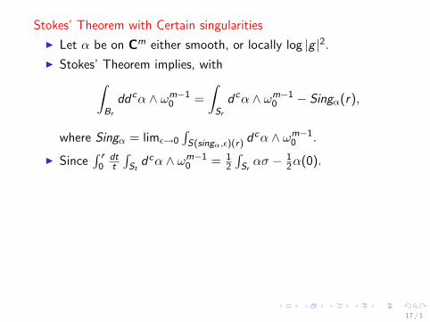
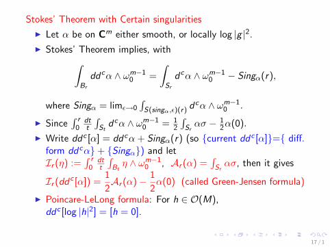
Stokes’ Theorem with Certain singularities

I Let α be on Cm either smooth, or locally log |g |2.

I Stokes’ Theorem implies, with∫Br

ddcα ∧ ωm−10 =

∫Sr

dcα ∧ ωm−10 − Singα(r),

where Singα = limε→0

∫S(singα,ε)(r) dcα ∧ ωm−1

0 .

I Since∫ r

0dtt

∫St

dcα ∧ ωm−10 = 1

2

∫Srασ − 1

2α(0).

I Write ddc [α] = ddcα + Singα(r) (so {current ddc [α]}={ diff.form ddcα}+ {Singα}) and letIr (η) :=

∫ r0

dtt

∫Btη ∧ ωm−1

0 , Ar (α) =∫Srασ, then it gives

Ir (ddc [α]) =1

2Ar (α)− 1

2α(0) (called Green-Jensen formula)

I Poincare-LeLong formula: For h ∈ O(M),ddc [log |h|2] = [h = 0].

17 / 1





∫Sr




0 .

I Since∫ r

0dtt

∫St

dcα ∧ ωm−10 = 1

2

∫Srασ − 1

2α(0).


∫ r0

dtt

∫Btη ∧ ωm−1


Ir (ddc [α]) =1

2Ar (α)− 1



17 / 1





∫Sr




0 .

I Since∫ r

0dtt

∫St

dcα ∧ ωm−10 = 1

2

∫Srασ − 1

2α(0).


∫ r0

dtt

∫Btη ∧ ωm−1


Ir (ddc [α]) =1

2Ar (α)− 1



17 / 1





∫Sr




0 .

I Since∫ r

0dtt

∫St

dcα ∧ ωm−10 = 1

2

∫Srασ − 1

2α(0).


∫ r0

dtt

∫Btη ∧ ωm−1


Ir (ddc [α]) =1

2Ar (α)− 1



17 / 1





∫Sr




0 .

I Since∫ r

0dtt

∫St

dcα ∧ ωm−10 = 1

2

∫Srασ − 1

2α(0).

I Write ddc [α] = ddcα + Singα(r) (so {current ddc [α]}={ diff.form ddcα}+ {Singα})

and letIr (η) :=

∫ r0

dtt

∫Btη ∧ ωm−1


Ir (ddc [α]) =1

2Ar (α)− 1



17 / 1





∫Sr




0 .

I Since∫ r

0dtt

∫St

dcα ∧ ωm−10 = 1

2

∫Srασ − 1

2α(0).


∫ r0

dtt

∫Btη ∧ ωm−1


Ir (ddc [α]) =1

2Ar (α)− 1



17 / 1





∫Sr




0 .

I Since∫ r

0dtt

∫St

dcα ∧ ωm−10 = 1

2

∫Srασ − 1

2α(0).


∫ r0

dtt

∫Btη ∧ ωm−1


Ir (ddc [α]) =1

2Ar (α)− 1



17 / 1





∫Sr




0 .

I Since∫ r

0dtt

∫St

dcα ∧ ωm−10 = 1

2

∫Srασ − 1

2α(0).


∫ r0

dtt

∫Btη ∧ ωm−1


Ir (ddc [α]) =1

2Ar (α)− 1



17 / 1

Averaging formula for growth functions

For any nondegeneratef : Cm → Pn, we have, in the sense of currents,f ∗ωk =

∫P∈Gn

kf −1(P)dµ(P), where µ is an measure on Gn

k which

is invariant under Un+1 and normalized with µ(Gnk ) = 1. Note

that P ∈ Gnk is a plane of codimension k passing though the origin

in Cn+1.It then implies the following averaging formula

Tk(r) =

∫Gn

k

Nf (P, r)dµ(P), k = 1, 2 . . . , n.

18 / 1

Averaging formula for growth functions For any nondegeneratef : Cm → Pn, we have, in the sense of currents,f ∗ωk =

∫P∈Gn


k which

is invariant under Un+1 and normalized with µ(Gnk ) = 1.

Notethat P ∈ Gn

k is a plane of codimension k passing though the originin Cn+1.It then implies the following averaging formula

Tk(r) =

∫Gn

k

Nf (P, r)dµ(P), k = 1, 2 . . . , n.

18 / 1


∫P∈Gn


k which



in Cn+1.

It then implies the following averaging formula

Tk(r) =

∫Gn

k

Nf (P, r)dµ(P), k = 1, 2 . . . , n.

18 / 1


∫P∈Gn


k which



in Cn+1.It then implies the following averaging formula

Tk(r) =

∫Gn

k

Nf (P, r)dµ(P), k = 1, 2 . . . , n.

18 / 1

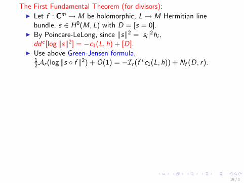
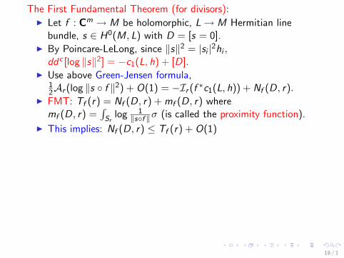
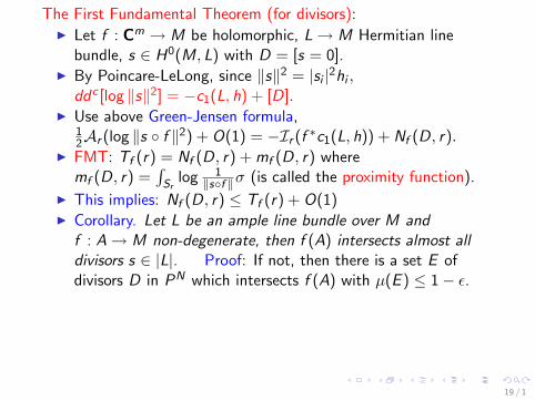
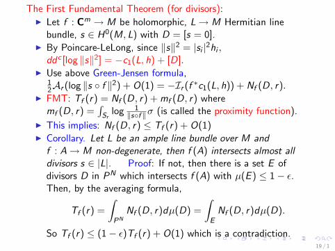
The First Fundamental Theorem (for divisors):

I Let f : Cm → M be holomorphic, L→ M Hermitian linebundle, s ∈ H0(M, L) with D = [s = 0].

I By Poincare-LeLong, since ‖s‖2 = |si |2hi ,ddc [log ‖s‖2] = −c1(L, h) + [D].

I Use above Green-Jensen formula,12Ar (log ‖s ◦ f ‖2) + O(1) = −Ir (f ∗c1(L, h)) + Nf (D, r).

I FMT: Tf (r) = Nf (D, r) + mf (D, r) wheremf (D, r) =

∫Sr

log 1‖s◦f ‖σ (is called the proximity function).

I This implies: Nf (D, r) ≤ Tf (r) + O(1)I Corollary. Let L be an ample line bundle over M and

f : A→ M non-degenerate, then f (A) intersects almost alldivisors s ∈ |L|. Proof: If not, then there is a set E ofdivisors D in PN which intersects f (A) with µ(E ) ≤ 1− ε.Then, by the averaging formula,

Tf (r) =

∫PN

Nf (D, r)dµ(D) =

∫E

Nf (D, r)dµ(D).

So Tf (r) ≤ (1− ε)Tf (r) + O(1) which is a contradiction.

19 / 1

The First Fundamental Theorem (for divisors):I Let f : Cm → M be holomorphic, L→ M Hermitian line

bundle, s ∈ H0(M, L) with D = [s = 0].

I By Poincare-LeLong, since ‖s‖2 = |si |2hi ,ddc [log ‖s‖2] = −c1(L, h) + [D].



∫Sr




Tf (r) =

∫PN

Nf (D, r)dµ(D) =

∫E

Nf (D, r)dµ(D).


19 / 1


bundle, s ∈ H0(M, L) with D = [s = 0].I By Poincare-LeLong, since ‖s‖2 = |si |2hi ,

ddc [log ‖s‖2] = −c1(L, h) + [D].



∫Sr




Tf (r) =

∫PN

Nf (D, r)dµ(D) =

∫E

Nf (D, r)dµ(D).


19 / 1



ddc [log ‖s‖2] = −c1(L, h) + [D].I Use above Green-Jensen formula,

12Ar (log ‖s ◦ f ‖2) + O(1) = −Ir (f ∗c1(L, h)) + Nf (D, r).


∫Sr




Tf (r) =

∫PN

Nf (D, r)dµ(D) =

∫E

Nf (D, r)dµ(D).


19 / 1






∫Sr




Tf (r) =

∫PN

Nf (D, r)dµ(D) =

∫E

Nf (D, r)dµ(D).


19 / 1






∫Sr


I This implies: Nf (D, r) ≤ Tf (r) + O(1)

I Corollary. Let L be an ample line bundle over M andf : A→ M non-degenerate, then f (A) intersects almost alldivisors s ∈ |L|. Proof: If not, then there is a set E ofdivisors D in PN which intersects f (A) with µ(E ) ≤ 1− ε.Then, by the averaging formula,

Tf (r) =

∫PN

Nf (D, r)dµ(D) =

∫E

Nf (D, r)dµ(D).


19 / 1






∫Sr



f : A→ M non-degenerate, then f (A) intersects almost alldivisors s ∈ |L|.

Proof: If not, then there is a set E ofdivisors D in PN which intersects f (A) with µ(E ) ≤ 1− ε.Then, by the averaging formula,

Tf (r) =

∫PN

Nf (D, r)dµ(D) =

∫E

Nf (D, r)dµ(D).


19 / 1






∫Sr



f : A→ M non-degenerate, then f (A) intersects almost alldivisors s ∈ |L|. Proof: If not, then there is a set E ofdivisors D in PN which intersects f (A) with µ(E ) ≤ 1− ε.

Then, by the averaging formula,

Tf (r) =

∫PN

Nf (D, r)dµ(D) =

∫E

Nf (D, r)dµ(D).


19 / 1






∫Sr




Tf (r) =

∫PN

Nf (D, r)dµ(D) =

∫E

Nf (D, r)dµ(D).


19 / 1






∫Sr




Tf (r) =

∫PN

Nf (D, r)dµ(D) =

∫E

Nf (D, r)dµ(D).

So Tf (r) ≤ (1− ε)Tf (r) + O(1) which is a contradiction.19 / 1

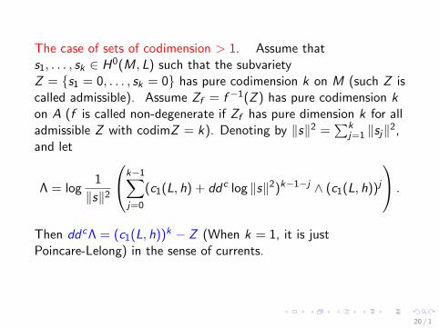
The case of sets of codimension > 1.

Assume thats1, . . . , sk ∈ H0(M, L) such that the subvarietyZ = {s1 = 0, . . . , sk = 0} has pure codimension k on M (such Z iscalled admissible). Assume Zf = f −1(Z ) has pure codimension kon A (f is called non-degenerate if Zf has pure dimension k for alladmissible Z with codimZ = k). Denoting by ‖s‖2 =

∑kj=1 ‖sj‖2,

and let

Λ = log1

‖s‖2

k−1∑j=0

(c1(L, h) + ddc log ‖s‖2)k−1−j ∧ (c1(L, h))j

.

Then ddcΛ = (c1(L, h))k − Z (When k = 1, it is justPoincare-Lelong) in the sense of currents.

20 / 1

The case of sets of codimension > 1. Assume thats1, . . . , sk ∈ H0(M, L) such that the subvarietyZ = {s1 = 0, . . . , sk = 0} has pure codimension k on M (such Z iscalled admissible).

Assume Zf = f −1(Z ) has pure codimension kon A (f is called non-degenerate if Zf has pure dimension k for alladmissible Z with codimZ = k). Denoting by ‖s‖2 =

∑kj=1 ‖sj‖2,

and let

Λ = log1

‖s‖2

k−1∑j=0


.


20 / 1

The case of sets of codimension > 1. Assume thats1, . . . , sk ∈ H0(M, L) such that the subvarietyZ = {s1 = 0, . . . , sk = 0} has pure codimension k on M (such Z iscalled admissible). Assume Zf = f −1(Z ) has pure codimension kon A (f is called non-degenerate if Zf has pure dimension k for alladmissible Z with codimZ = k).

Denoting by ‖s‖2 =∑k

j=1 ‖sj‖2,and let

Λ = log1

‖s‖2

k−1∑j=0


.


20 / 1

The case of sets of codimension > 1. Assume thats1, . . . , sk ∈ H0(M, L) such that the subvarietyZ = {s1 = 0, . . . , sk = 0} has pure codimension k on M (such Z iscalled admissible). Assume Zf = f −1(Z ) has pure codimension kon A (f is called non-degenerate if Zf has pure dimension k for alladmissible Z with codimZ = k). Denoting by ‖s‖2 =

∑kj=1 ‖sj‖2,

and let

Λ = log1

‖s‖2

k−1∑j=0


.


20 / 1

FMT for codimension k > 1:

If f : A→ M is non-degenerate, then

mf (Z , r) + Nf (Z , r) = Tk(r) + Rk(Z , r) + O(1),

orNf (Z , r) < Tk(r) + Rk(Z , r) + O(1),

where

mf (Z , r) =

∫∂A[r ]

f ∗(Λ) ∧ σk ,

where σk = dcτ ∧ ωm−k0 ,

Rk(Z , r) =1

2

∫∂A[r ]

f ∗(Λ) ∧ ωm−k+10 (supplementary term).

21 / 1

FMT for codimension k > 1: If f : A→ M is non-degenerate, then


orNf (Z , r) < Tk(r) + Rk(Z , r) + O(1),

where

mf (Z , r) =

∫∂A[r ]

f ∗(Λ) ∧ σk ,


Rk(Z , r) =1

2

∫∂A[r ]


21 / 1



orNf (Z , r) < Tk(r) + Rk(Z , r) + O(1),

where

mf (Z , r) =

∫∂A[r ]

f ∗(Λ) ∧ σk ,


Rk(Z , r) =1

2

∫∂A[r ]


21 / 1



orNf (Z , r) < Tk(r) + Rk(Z , r) + O(1),

where

mf (Z , r) =

∫∂A[r ]

f ∗(Λ) ∧ σk ,


Rk(Z , r) =1

2

∫∂A[r ]


21 / 1



orNf (Z , r) < Tk(r) + Rk(Z , r) + O(1),

where

mf (Z , r) =

∫∂A[r ]

f ∗(Λ) ∧ σk ,


Rk(Z , r) =1

2

∫∂A[r ]


21 / 1

Averaging and density theorems

I Using∫{Z}

Rk(Z , r)dµ(Z ) = c

∫A[r ]

(f ∗c1(L, h))k−1∧ωm−k+10 = ctk−1(r),

and using the averaging formula for the order function (similarto above), we have the following result due to Chern, Stolland Wu:

I Theorem: Assume that

lim infr→∞

tk−1(r)

Tk(r)= 0.

Then the image f (A) meets almost all Z (s) for s ∈ G (k,N).In particular, the image f (A) meets almost all divisors D ∈ |L|.

22 / 1


I Using∫{Z}


∫A[r ]

(f ∗c1(L, h))k−1∧ωm−k+10 = ctk−1(r),



lim infr→∞

tk−1(r)

Tk(r)= 0.


22 / 1


I Using∫{Z}


∫A[r ]

(f ∗c1(L, h))k−1∧ωm−k+10 = ctk−1(r),



lim infr→∞

tk−1(r)

Tk(r)= 0.

Then the image f (A) meets almost all Z (s) for s ∈ G (k,N).

In particular, the image f (A) meets almost all divisors D ∈ |L|.

22 / 1


I Using∫{Z}


∫A[r ]

(f ∗c1(L, h))k−1∧ωm−k+10 = ctk−1(r),



lim infr→∞

tk−1(r)

Tk(r)= 0.


22 / 1

Documents

Introduction to Nevanlinna theoryminru/talk1.pdfIntroduction: The algebraic case I The well-known fundamental theorem of algebra states that, for every complex polynomial P, deg P