Embed Size (px)
Citation preview
Diophantine Approximation and NevanlinnaTheory
Paul Vojta
Abstract As was originally observed by C. F. Osgood and further developed by theauthor, there is a formal analogy between Nevanlinna theory in complex analysisand certain results in diophantine approximation. These notes describe this analogy,after briefly introducing the theory of heights and Weil function in number theoryand the main concepts of Nevanlinna theory. Parallel conjectures are then presented,in Nevanlinna theory (“Griffiths’ conjecture”) and the author’s conjecture on ratio-nal points. Following this, recent work is described, highlighting work of Corvaja,Zannier, Evertse, and Ferretti on combining Schmidt’s Subspace Theorem with ge-ometrical constructions to obtain partial results on this conjecture. Counterparts ofthese results in Nevanlinna theory are also given (due to Ru). These notes also de-scribe parallel extensions of the conjectures in Nevanlinna theory and diophantineapproximation, to involve finite ramified coverings and algebraic points, respec-tively. Variants of these conjectures involving truncated counting functions are alsointroduced, and the relations of these various conjectures with the abc conjecture ofMasser and Oesterle are also described.
0 Introduction
Beginning with the work of C. F. Osgood [1981], it has been known that the branchof complex analysis known as Nevanlinna theory (also called value distribution the-ory) has many similarities with Roth’s theorem on diophantine approximation. Thiswas extended by the author [Vojta, 1987] to include an explicit dictionary and to in-clude geometric results as well, such as Picard’s theorem and Mordell’s conjecture(Faltings’ theorem). The latter analogy ties in with Lang’s conjecture that a projec-
Paul VojtaDepartment of Mathematics, University of California, 970 Evans Hall #3840, Berkeley, CA 94720-3840 e-mail: [email protected] supported by NSF grant DMS-0500512
113
114 Paul Vojta
tive variety should have only finitely many rational points over any given numberfield (i.e., is Mordellic) if and only if it is Kobayashi hyperbolic.
This circle of ideas has developed further in the last 20 years: Lang’s conjectureon sharpening the error term in Roth’s theorem was carried over to a conjecture inNevanlinna theory which was proved in many cases. In the other direction, Bloch’sconjectures on holomorphic curves in abelian varieties (later proved; see Section14 for details) led to proofs of the corresponding results in number theory (again,see Section 14). More recently, work in number theory using Schmidt’s SubspaceTheorem has led to corresponding results in Nevanlinna theory.
This relation with Nevanlinna theory is in some sense similar to the (much older)relation with function fields, in that one often looks to function fields or Nevanlinnatheory for ideas that might translate over to the number field case, and that workover function fields or in Nevanlinna theory is often easier than work in the numberfield case. On the other hand, both function fields and Nevanlinna theory have con-cepts that (so far) have no counterpart in the number field case. This is especiallytrue of derivatives, which exist in both the function field case and in Nevanlinnatheory. In the number field case, however, one would want the “derivative with re-spect to p,” which remains as a major stumbling block, although (separate) work ofBuium and of Minhyong Kim may ultimately provide some answers. The search forsuch a derivative is also addressed in these notes, using a potential approach usingsuccessive minima.
It is important to note, however, that the relation with Nevanlinna theory does not“go through” the function field case. Although it is possible to look at the functionfield case over C and apply Nevanlinna theory to the functions representing therational points, this is not the analogy being described here. Instead, in the analogypresented here, one holomorphic function corresponds to infinitely many rational oralgebraic points (whether over a number field or over a function field). Thus, theanalogy with Nevanlinna theory is less concrete, and may be regarded as a moredistant analogy than function fields.
These notes describe some of the work in this area, including much of the nec-essary background in diophantine geometry. Specifically, Sections 1–3 recall basicdefinitions of number theory and the theory of heights of elements of number fields,culminating in the statement of Roth’s theorem and some equivalent formulations ofthat theorem. This part assumes that the reader knows the basics of algebraic numbertheory and algebraic geometry at the level of Lang [1970] and Hartshorne [1977],respectively. Some proofs are omitted, however; for those the interested reader mayrefer to Lang [1983].
Sections 4–6 briefly introduce Nevanlinna theory and the analogy between Roth’stheorem and the classical work of Nevanlinna. Again, many proofs are omitted;references include Shabat [1985], Nevanlinna [1970], and Goldberg and Ostrovskii[2008] for pure Nevanlinna theory, and Vojta [1987] and Ru [2001] for the analogy.
Sections 7–15 generalize the content of the earlier sections, in the more geometriccontext of varieties over the appropriate fields (number fields, function fields, or C).Again, proofs are often omitted; most may be found in the references given above.
Diophantine Approximation and Nevanlinna Theory 115
Section 14 in particular introduces the main conjectures being discussed here:Conjecture 14.2 in Nevanlinna theory (“Griffiths’ conjecture”) and its counterpartin number theory, the author’s Conjecture 14.6 on rational points on varieties.
Sections 16 and 17 round out the first part of these notes, by discussing the func-tion field case and the subject of the exceptional sets that come up in the study ofhigher dimensional varieties.
In both Nevanlinna theory and number theory, these conjectures have beenproved only in very special cases, mostly involving subvarieties of semiabelian va-rieties. This includes the case of projective space minus a collection of hyperplanesin general position (Cartan’s theorem and Schmidt’s Subspace Theorem). Recentwork of Corvaja, Zannier, Evertse, Ferretti, and Ru has shown, however, that usinggeometric constructions one can use Schmidt’s Subspace Theorem and Cartan’s the-orem to derive other weak special cases of the conjectures mentioned above. This isthe subject of Sections 18–22.
Sections 23–27 present generalizations of Conjectures 14.2 and 14.6. Conjecture14.2, in Nevanlinna theory, can be generalized to involve truncated counting func-tions (as was done by Nevanlinna in the 1-dimensional case), and can also be posedin the context of finite ramified coverings. In number theory, Conjecture 14.6 canalso be generalized to involve truncated counting functions. The simplest nontrivialcase of this conjecture, involving the divisor [0]+ [1]+ [∞] on P1, is the celebrated“abc conjecture” of Masser and Oesterle. Thus, Conjecture 22.5 can be regardedas a generalization of the abc conjecture as well as of Conjecture 14.6. One canalso generalize Conjecture 14.6 to treat algebraic points; this corresponds to finiteramified coverings in Nevanlinna theory. This is Conjecture 24.1, which can also beposed using truncated counting functions (Conjecture 24.3).
Sections 28 and 29 briefly discuss the question of derivatives in Nevanlinna the-ory, and Nevanlinna’s “Lemma on the Logarithmic Derivative.” A geometric formof this lemma, due to R. Kobayashi, M. McQuillan, and P.-M. Wong, is given, and itis shown how this form leads to an inequality in Nevanlinna theory, due to McQuil-lan, called the “tautological inequality.” This inequality then leads to a conjecture innumber theory (Conjecture 29.1), which of course should then be called the “tauto-logical conjecture.” This conjecture is discussed briefly; it is of interest since it mayshed some light on how one might take “derivatives” in number theory.
The abc conjecture infuses much of this theory, not only because a Nevanlinna-like conjecture with truncated counting functions contains the abc conjecture as aspecial case, but also because other conjectures also imply the abc conjecture, andtherefore are “at least as hard” as abc. Specifically, Conjecture 24.1, on algebraicpoints, implies the abc conjecture, even if known only in dimension 1, and Con-jecture 14.6, on rational points, also implies abc if known in high dimensions. Thislatter implication is the subject of Section 30. Finally, implications in the other di-rection are explored in Section 31.
116 Paul Vojta
1 Notation and Basic Results: Number Theory
We assume that the reader has an understanding of the fundamental basic factsof number theory (and algebraic geometry), up through the definitions of (Weil)heights. References for these topics include [Lang, 1983] and [Vojta, 1987]. Wedo, however, recall some of the basic conventions here since they often differ fromauthor to author.
Throughout these notes, k will usually denote a number field; if so, then Ok willdenote its ring of integers and Mk its set of places. This latter set is in one-to-onecorrespondence with the disjoint union of the set of nonzero prime ideals of Ok,the set of real embeddings σ : k → R, and the set of unordered complex conjugatepairs (σ ,σ) of complex embeddings σ : k → C with image not contained in R.Such elements of Mk are called non-archimedean or finite places, real places, andcomplex places, respectively.
The real and complex places are collectively referred to as archimedean or infi-nite places. The set of these places is denoted S∞. It is a finite set.
To each place v ∈Mk we associate a norm ‖ ·‖v, defined for x ∈ k by ‖x‖v = 0 ifx = 0 and(1.1)
‖x‖v =
(Ok : p)ordp(x) if v corresponds to p⊆ Ok;|σ(x)| if v corresponds to σ : k → R; and|σ(x)|2 if v is a complex place, corresponding to σ : k → C
if x 6= 0. Here ordp(x) means the exponent of p in the factorization of the fractionalideal (x). If we use the convention that ordp(0) = ∞, then (1.1) is also valid whenx = 0.
We refer to ‖ · ‖v as a norm instead of an absolute value, because ‖ · ‖v does notsatisfy the triangle inequality when v is a complex place. However, let
(1.2) Nv =
0 if v is non-archimedean;1 if v is real; and2 if v is complex.
Then the norm associated to a place v of k satisfies the axioms
(1.3.1) ‖x‖v ≥ 0, with equality if and only if x = 0;(1.3.2) ‖xy‖v = ‖x‖v‖y‖v for all x,y ∈ k; and(1.3.3) ‖x1 + · · ·+ xn‖v ≤ nNv max‖x1‖v, . . . ,‖xn‖v for all x1, . . . ,xn ∈ k, n ∈ N.
(In these notes, N = 0,1,2, . . ..)Some authors treat complex conjugate embeddings as distinct places. We do not
do so here, because they give rise to the same norms.Note that, if x ∈ k, then x lies in the ring of integers if and only if ‖x‖v ≤ 1 for
all non-archimedean places v. Indeed, if x 6= 0 then both conditions are equivalentto the fractional ideal (x) being a genuine ideal.
Diophantine Approximation and Nevanlinna Theory 117
Let L be a finite extension of a number field k, and let w be a place of L. If w isnon-archimedean, corresponding to a nonzero prime ideal q⊆OL, then p := q∩Okis a nonzero prime of Ok, and gives rise to a non-archimedean place v ∈ Mk. If varises from w in this way, then we say that w lies over v, and write w | v. Likewise, ifw is archimedean, then it corresponds to an embedding τ : L →C, and its restrictionτ∣∣k : k → C gives rise to a unique archimedean place v ∈Mk, and again we say that
w lies over v and write w | v.For each v ∈Mk, the set of w ∈ML lying over it is nonempty and finite. If w | v
then we also say that v lies under w.If S is a subset of Mk, then we say w | S if w lies over some place in S; otherwise
we write w - S.If w | v, then we have
(1.4) ‖x‖w = ‖x‖[Lw:kv]v for all x ∈ k ,
where Lw and kv denote the completions of L and k at w and v, respectively. We alsohave
(1.5) ∏w∈ML
w|v
‖y‖w = ‖NLk y‖v for all v ∈Mk and all y ∈ L .
This is proved by using the isomorphism L⊗k kv ∼= ∏w|v Lw; see for example[Neukirch, 1999, Ch. II, Cor. 8.4].
Let L/K/k be a tower of number fields, and let w′ and v be places of L and k,respectively. Then w′ | v if and only if there is a place w of K satisfying w′ | w andw | v.
The field k = Q has no complex places, one real place corresponding to the inclu-sion Q ⊆ R, and infinitely many non-archimedean places, corresponding to primerational integers. Thus, we write
MQ = ∞,2,3,5, . . . .
Places of a number field satisfy a Product Formula
(1.6) ∏v∈Mk
‖x‖v = 1 for all x ∈ k∗ .
This formula plays a key role in number theory: it is used to show that certain ex-pressions for the height are well defined, and it also implies that if ∏v ‖x‖v < 1 thenx = 0.
The Product Formula is proved first by showing that it is true when k = Q (bydirect verification) and then using (1.5) to pass to an arbitrary number field.
118 Paul Vojta
2 Heights
The height of a number, or of a point on a variety, is a measure of the complexity ofthat number. For example, 100/201 and 1/2 are very close to each other (using thenorm at the infinite place, at least), but the latter is a much “simpler” number sinceit can be written down using fewer digits.
We define the height (also called the Weil height) of an element x ∈ k by theformula
(2.1) Hk(x) = ∏v∈Mk
max‖x‖v,1 .
As an example, consider the special case in which k = Q. Write x = a/b with a,b∈Zrelatively prime. For all (finite) rational primes p, if pi is the largest power of pdividing a, and p j is the largest power dividing b, then ‖a‖p = p−i and ‖b‖p = p− j,and therefore max‖x‖p,1 = pb. Therefore the product of all terms in (2.1) overall finite places v is just |b|. At the infinite place, we have ‖x‖∞ = |a/b|, so this gives
(2.2) HQ(x) = max|a|, |b| .
Similarly, if P ∈ Pn(k) for some n ∈ N, we define the Weil height hk(P) as fol-lows. Let [x0 : · · · : xn] be homogeneous coordinates for P (with the xi always as-sumed to lie in k). Then we define
(2.3) Hk(P) = ∏v∈Mk
max‖x0‖v, . . . ,‖xn‖v .
By the Product Formula (1.6), this quantity is independent of the choice of homo-geneous coordinates.
If we identify k with A1(k) and identify the latter with a subset of P1(k) via thestandard injection i : A1 → P1, then we note that Hk(x) = Hk(i(x)) for all x ∈ k.Similarly, we can identify kn with An(k), and the standard embedding of An into Pn
gives us a height
Hk(x1, . . . ,xn) = ∏v∈Mk
max‖x1‖v, . . . ,‖xn‖v,1 .
The height functions defined so far, all using capital ‘H,’ are called multiplicativeheights. Usually it is more convenient to take their logarithms and define logarith-mic heights:
(2.4) hk(x) = logHk(x) = ∑v∈Mk
log+ ‖x‖v
and
hk([x0 : · · · : xn]) = logHk([x0 : · · · : xn]) = ∑v∈Mk
logmax‖x0‖v, . . . ,‖xn‖v .
Diophantine Approximation and Nevanlinna Theory 119
Herelog+(x) = maxlogx,0 .
The equation (1.5) tells us how heights change when the number field k is ex-tended to a larger number field L:
(2.5) hL(x) = [L : k]hk(x)
and
(2.6) hL([x0 : · · · : xn]) = [L : k]hk([x0 : · · · : xn])
for all x ∈ k and all [x0, . . . ,xn] ∈ Pn(k), respectively.Then, given x ∈Q, we define
hk(x) =1
[L : k]hL(x)
for any number field L ⊇ k(x), and similarly given any [x0 : · · · : xn] ∈ Pn(Q), wedefine
hk([x0 : · · · : xn]) =1
[L : k]hL([x0 : · · · : xn])
for any number field L ⊇ k(x0, . . . ,xn). These expressions are independent of thechoice of L by (2.5) and (2.6), respectively.
Following EGA, if x is a point on Pnk , then κ(x) will denote the residue field of
the local ring at x. If x is a closed point then the homogeneous coordinates can bechosen such that k(x0, . . . ,xn) = κ(x).
With these definitions, (2.5) and (2.6) remain valid without the conditions x ∈ kand [x0 : · · · : xn] ∈ Pn(k), respectively.
It is common to assume k = Q and omit the subscript k. The resulting heights arecalled absolute heights.
It is obvious from (2.1) that hk(x) ≥ 0 for all x ∈ k, and that equality holds ifx = 0 or if x is a root of unity. Conversely, hk(x) = 0 implies ‖x‖v ≤ 1 for all v; ifx 6= 0 then the Product Formula implies ‖x‖v = 1 for all v. Thus x must be a unit,and the known structure of the unit group then leads to the fact that x must be a rootof unity.
Therefore, there are infinitely many elements of Q with height 0. If one boundsthe degree of such elements over Q, then there are only finitely many; more gener-ally, we have:
Theorem 2.7. (Northcott’s finiteness theorem) For any r ∈ Z>0 and any C ∈ R,there are only finitely many x ∈Q such that [Q(x) : Q]≤ r and h(x)≤C. Moreover,given any n ∈N there are only finitely many x ∈ Pn(Q) such that [κ(x) : Q]≤ r andh(x)≤C.
The first assertion is proved using the fact that, for any x∈Q, if one lets k = Q(x),then Hk(x) is within a constant factor of the largest absolute value of the largest coef-ficient of the irreducible polynomial of x over Q, when that polynomial is multiplied
120 Paul Vojta
by a rational number so that its coefficients are relatively prime integers. The sec-ond assertion then follows as a consequence of the first. For details, see [Lang, 1991,Ch. II, Thm. 2.2].
This result plays a central role in number theory, since (for example) proving anupper bound on the heights of rational points is equivalent to proving finiteness.
3 Roth’s Theorem
K. F. Roth [1955] proved a key and much-anticipated theorem on how well an alge-braic number can be approximated by rational numbers. Of course rational numbersare dense in the reals, but if one limits the size of the denominator then one can askmeaningful and nontrivial questions.
Theorem 3.1. (Roth) Fix α ∈Q, ε > 0, and C > 0. Then there are only finitely manya/b ∈Q, where a and b are relatively prime integers, such that
(3.1.1)∣∣∣ab−α
∣∣∣≤ C|b|2+ε
.
Example 3.2. As a diophantine application of Roth’s theorem, consider the diophan-tine equation
(3.2.1) x3−2y3 = 11, x,y ∈ Z .
If (x,y) is a solution, then x/y must be close to 3√2 (assuming |x| or |y| is large,which would imply both are large):∣∣∣∣xy − 3√2
∣∣∣∣= ∣∣∣∣ 11y(x2 + xy 3√2+ y2 3√4)
∣∣∣∣ 1|y|3
.
Thus Roth’s theorem implies that (3.2.1) has only finitely many solutions.More generally, if f ∈ Z[x,y] is homogeneous of degree ≥ 3 and has no repeated
factors, then for any a ∈ Z f (x,y) = a has only finitely many integral solutions.This is called the Thue equation and historically was the driving force behind thedevelopment of Roth’s theorem (which is sometimes called the Thue-Siegel-Roththeorem, sometimes also mentioning Schneider, Dyson, and Mahler).
The inequality (3.1.1) is best possible, in the sense that the 2 in the exponenton the right-hand side cannot be replaced by a smaller number. This can be shownusing continued fractions. Of course one can conjecture a sharper error term [Langand Cherry, 1990, Intro. to Ch. I].
If a/b is close to α , then after adjusting C one can replace |b| in the right-handside of (3.1.1) with HQ(a/b) (see (2.2)). Moreover, the theorem has been general-ized to allow a finite set of places (possibly non-archimedean) and to work over anumber field:
Diophantine Approximation and Nevanlinna Theory 121
Theorem 3.3. Let k be a number field, let S be a finite set of places of k containingall archimedean places, fix αv ∈ Q for each v ∈ S, let ε > 0, and let C > 0. Thenonly finitely many x ∈ k satisfy the inequality
(3.3.1) ∏v∈S
min1,‖x−αv‖v ≤C
Hk(x)2+ε.
(Strictly speaking, S can be any finite set of places at this point, but requiring S tocontain all archimedean places does not weaken the theorem, and this assumptionwill be necessary in Section 5. See, for example, (5.3).)
Taking− log of both sides of (3.3.1), dividing by [k : Q], and rephrasing the logic,the above theorem is equivalent to the assertion that for all c ∈ R the inequality
(3.4)1
[k : Q] ∑v∈S
log+∥∥∥∥ 1
x−αv
∥∥∥∥v≤ (2+ ε)h(x)+ c
holds for all but finitely many x ∈ k.In writing (3.3.1), we assume that one has chosen an embedding iv : k → kv over
k for each v ∈ S. Otherwise the expression ‖x−αv‖v may not make sense.This is mostly a moot point, however, since we may restrict to αv ∈ k for
all v. Clearly this restricted theorem is implied by the theorem without the ad-ditional restriction, but in fact it also implies the original theorem. To see this,suppose k, S, ε , and c are as above, and assume that αv ∈ Q are given for allv ∈ S. Let L be the Galois closure over k of k(αv : v ∈ S), and let T be the setof all places of L lying over places in S. We assume that L is a subfield of k,so that αv ∈ L for all v ∈ S. Then (iv)
∣∣L : L → kv induces a place w0 of L over
v, and all other places w of L over v are conjugates by elements σw ∈ Gal(L/k):‖x‖w = ‖σ−1
w (x)‖w0 for all x ∈ L. Letting αw = σw(αv) for all w | v, we then have
‖x−αw‖w = ‖σ−1w (x−αw)‖w0 = ‖x−αv‖
[Lw0 :kv]v for all x∈ k by (1.4), and therefore
∑w|v
log+∥∥∥∥ 1
x−αw
∥∥∥∥w
= ∑w|v
[Lw0 : kv] log+∥∥∥∥ 1
x−αv
∥∥∥∥v= [L : k] log+
∥∥∥∥ 1x−αv
∥∥∥∥v
since L/k is Galois. Thus
1[k : Q] ∑
v∈Slog+
∥∥∥∥ 1x−αv
∥∥∥∥v=
1[L : Q] ∑
w∈Tlog+
∥∥∥∥ 1x−αw
∥∥∥∥w
for all x ∈ k. Applying Roth’s theorem over the field L (where now αw ∈ L for allw ∈ T ) then gives (3.4) for almost all x ∈ k.
Finally, we note that Roth’s theorem (as now rephrased) is equivalent to the fol-lowing statement.
Theorem 3.5. Let k be a number field, let S ⊇ S∞ be a finite set of places of k, fixdistinct α1, . . . ,αq ∈ k, let ε > 0, and let c ∈ R. Then the inequality
122 Paul Vojta
(3.5.1)1
[k : Q] ∑v∈S
q
∑i=1
log+∥∥∥∥ 1
x−αi
∥∥∥∥v≤ (2+ ε)h(x)+ c
holds for almost all x ∈ k.
Indeed, given αv ∈ k for all v ∈ S, let α1, . . . ,αq be the distinct elements of theset αv : v ∈ S. Then
1[k : Q] ∑
v∈Slog+
∥∥∥∥ 1x−αv
∥∥∥∥v≤ 1
[k : Q] ∑v∈S
q
∑i=1
log+∥∥∥∥ 1
x−αi
∥∥∥∥v,
so Theorem 3.5 implies the earlier form of Roth’s theorem (as modified).Conversely, given distinct α1, . . . ,αq ∈ k, we note that any given x ∈ k can be
close to only one of the αi at each place v (where the value of i may depend on v).Therefore, for each v,
q
∑i=1
log+∥∥∥∥ 1
x−αi
∥∥∥∥v≤ log+
∥∥∥∥ 1x−αv
∥∥∥∥v+ cv
for some constant cv independent of x and some αv ∈ α1, . . . ,αq depending on xand v. Thus, for each x ∈ k, there is a choice of αv for each v ∈ S such that
1[k : Q] ∑
v∈S
q
∑i=1
log+∥∥∥∥ 1
x−αi
∥∥∥∥v≤ 1
[k : Q] ∑v∈S
log+∥∥∥∥ 1
x−αv
∥∥∥∥v+ c′ ,
where c′ is independent of x. Since there are only finitely many choices of the systemαv : v ∈ S, finitely many applications of the earlier version of Roth’s theoremsuffice to imply Theorem 3.5.
4 Basics of Nevanlinna Theory
Nevanlinna theory, developed by R. and F. Nevanlinna in the 1920s, concerns thedistribution of values of holomorphic and meromorphic functions, in much the sameway that Roth’s theorem concerns approximation of elements of a number field.
One can think of it as a generalization of a theorem of Picard, which says that anonconstant holomorphic function from C to P1 can omit at most two points. This,in turn, generalizes Liouville’s theorem.
An example relevant to Picard’s theorem is the exponential function ez, whichomits the values 0 and ∞. When r is large, the circle |z| = r is mapped to manyvalues close to ∞ (when Rez is large) and many values close to 0 (when Rez ishighly negative).
So even though ez omits these two values, it spends a lot of time very close tothem. This observation can be made precise, in what is called Nevanlinna’s FirstMain Theorem. In order to state this theorem, we need some definitions.
Diophantine Approximation and Nevanlinna Theory 123
First we recall that log+ x = maxlogx,0, and similarly define
ord+z f = maxordz f ,0
if f is a meromorphic function and z ∈ C.
Definition 4.1. Let f be a meromorphic function on C. We define the proximityfunction of f by
(4.1.1) m f (r) =∫ 2π
0log+∣∣ f (reiθ )
∣∣ dθ
2π
for all r > 0. We also define
m f (∞,r) = m f (r) and m f (a,r) = m1/( f−a)(r)
when a ∈ C.
The integral in (4.1.1) converges when f has a zero or pole on the circle |z|= r,so it is defined everywhere. The proximity function m f (a,r) is large to the extentthat the values of f on |z|= r are close to a.
Definition 4.2. Let f be a meromorphic function on C. For r > 0 let n f (r) be thenumber of poles of f in the open disc |z|< r of radius r (counted with multiplicity),and let n f (0) be the order of the pole (if any) at z = 0. We then define the countingfunction of f by
(4.2.1) N f (r) =∫ r
0(n f (s)−n f (0))
dss
+n f (0) logr .
As before, we also define
N f (∞,r) = N f (r) and N f (a,r) = N1/( f−a)(r)
when a ∈ C.
The counting function can also be written
(4.3) N f (a,r) = ∑0<|z|<r
ord+z ( f −a) · log
r|z|
+ord+0 ( f −a) · logr .
Thus, the expression N f (a,r) is a weighted count, with multiplicity, of the numberof times f takes on the value a in the disc |z|< r.
Definition 4.4. Let f be as in Definition 4.1. Then the height function of f is thefunction Tf : (0,∞)→ R given by
(4.4.1) Tf (r) = m f (r)+N f (r) .
124 Paul Vojta
Classically, the above function is called the characteristic function, but here wewill use the term height function, since this is more in parallel with terminology inthe number field case. The height function Tf does, in fact, measure the complexityof the meromorphic function f .
In particular, if f is constant then so is Tf (r); otherwise,
(4.5) liminfr→∞
Tf (r)logr
> 0 .
Moreover, it is known that Tf (r) = O(logr) if and only if f is a rational func-tion. Although this is a well-known fact, I was unable to find a convenient refer-ence, so a proof is sketched here. If f is rational, then direct computation givesTf (r) = O(logr). Conversely, if Tf (r) = O(logr) then f can have only finitelymany poles; clearing these by multiplying f by a polynomial changes Tf by at mostO(logr), so we may assume that f is entire. We may also assume that f is non-constant. By [Hayman, 1964, Thm. 1.8], if f is entire and nonconstant and K > 1,then
liminfr→∞
logmax|z|=r | f (z)|Tf (r)(logTf (r))K = 0 .
This implies that f (z)/zn has a removable singularity at ∞ for sufficiently large n,hence is a polynomial.
The following theorem relates the height function to the proximity and countingfunctions at points other than ∞.
Theorem 4.6. (First Main Theorem) Let f be a meromorphic function on C, and leta ∈ C. Then
Tf (r) = m f (a,r)+N f (a,r)+O(1) ,
where the constant in O(1) depends only on f and a.
This theorem is a straightforward consequence of Jensen’s formula
log |c f |=∫ 2π
0log∣∣ f (reiθ )
∣∣ dθ
2π+N f (∞,r)−N f (0,r) ,
where c f is the leading coefficient in the Laurent expansion of f at z = 0. For details,see [Nevanlinna, 1970, Ch. VI, (1.2’)] or [Ru, 2001, Cor. A1.1.3].
As an example, let f (z) = ez. This function is entire, so N f (∞,r) = 0 for all r.We also have
m f (∞,r) =∫ 2π
0log+ er cosθ dθ
2π= r
∫π/2
−π/2cosθ
dθ
2π=
rπ
.
ThusTf (r) =
rπ
.
Similarly, we have N f (0,r) = 0 and m f (0,r) = r/π for all r, confirming the FirstMain Theorem in the case a = 0.
Diophantine Approximation and Nevanlinna Theory 125
The situation with a =−1 is more difficult. The integral in the proximity functionseems to be beyond any hope of computing exactly. Since ez = −1 if and only if zis an odd integral multiple of πi, we have
N f (−1,r) = 2∫ r
0
[s
2π+
12
]dss≈ 2
∫ r
0
s2π
dss
=rπ
,
where [ · ] denotes the greatest integer function. The error in the above approximationshould be o(r), which would give m(−1,r) = o(r). Judging from the general shapeof the exponential function, similar estimates should hold for all nonzero a ∈ C.
In one way of thinking, the First Main Theorem gives an upper bound on thecounting function. As the above example illustrates, there is no lower bound foran individual counting function (other than 0), but it is known that there cannot bemany values of a for which N f (a,r) is much smaller than the height. This is whatthe Second Main Theorem shows.
Theorem 4.7. (Second Main Theorem) Let f be a meromorphic function on C, andlet a1, . . . ,aq ∈ C be distinct numbers. Then
(4.7.1)q
∑j=1
m f (a j,r)≤exc 2Tf (r)+O(log+ Tf (r))+o(logr) ,
where the implicit constants depend only on f and a1, . . . ,aq.
Here the notation ≤exc means that the inequality holds for all r > 0 outside of aset of finite Lebesgue measure.
By the First Main Theorem, (4.7.1) can be rewritten as a lower bound on thecounting functions:
(4.8)q
∑j=1
N f (a j,r)≥exc (q−2)Tf (r)−O(log+ Tf (r))−o(logr) .
As another variation, (4.7.1) can be written with a weaker error term:
(4.9)q
∑j=1
m f (a j,r)≤exc (2+ ε)Tf (r)+ c
for all ε > 0 and any constant c. The next section will show that this correponds toRoth’s theorem.
Corollary 4.10. (Picard’s “little” theorem) If a1,a2,a3 ∈ P1(C) are distinct, thenany holomorphic function f : C→ P1(C)\a1,a2,a3 must be constant.
Proof. Assume that f : C→P1(C)\a1,a2,a3 is a nonconstant holomorphic func-tion. After applying an automorphism of P1 if necessary, we may assume that all a jare finite. We may regard f as a meromorphic function on C.
126 Paul Vojta
Since f never takes on the values a1, a2, or a3, the left-hand side of (4.8) van-ishes. Since f is nonconstant, the right-hand side approaches +∞ by (4.5). This is acontradiction. ut
As we have seen, (4.8) has some advantages over (4.7.1). Other advantages in-clude the fact that q−2 on the right-hand side is the Euler characteristic of P1 minusq points, and it will become clear later that the dependence on a metric is restrictedto the height term. It is also the preferred form when comparing with the abc con-jecture.
5 Roth’s Theorem and Nevanlinna Theory
We now claim that Nevanlinna’s Second Main Theorem corresponds very closely toRoth’s theorem. To see this, we make the following definitions in number theory.
Definition 5.1. Let k be a number field and S ⊇ S∞ a finite set of places of k. Forx ∈ k we define the proximity function to be
mS(x) = ∑v∈S
log+ ‖x‖v
and, for a ∈ k with a 6= x,
(5.1.1) mS(a,x) = mS
(1
x−a
)= ∑
v∈Slog+
∥∥∥∥ 1x−a
∥∥∥∥v.
Similarly, for distinct a,x ∈ k the counting function is defined as
NS(x) = ∑v/∈S
log+ ‖x‖v
and
(5.1.2) NS(a,x) = NS
(1
x−a
)= ∑
v/∈Slog+
∥∥∥∥ 1x−a
∥∥∥∥v.
By (2.4) it then follows that
(5.2) mS(x)+NS(x) = ∑v∈Mk
log+ ‖x‖v = hk(x)
for all x ∈ k. This corresponds to (4.4.1).Note that k does not appear in the notation for the proximity and counting func-
tions, since it is implied by S.We also note that all places outside of S are non-archimedean, hence correspond
to nonzero prime ideals p⊆ Ok. Thus, by (1.1), (5.1.2) can be rewritten
Diophantine Approximation and Nevanlinna Theory 127
(5.3) NS(a,x) = ∑v/∈S
ord+p (x−a) · log(Ok : p) ,
where p in the summand is the prime ideal corresponding to v. This corresponds to(4.3).
The number field case has an analogue of the First Main Theorem, which weprove as follows.
Lemma 5.4. Let v be a place of a number field k, and let a,x ∈ k. Then
(5.4.1)∣∣∣log+ ‖x‖v− log+ ‖x−a‖v
∣∣∣≤ log+ ‖a‖v +Nv log2 .
Proof. Case I: v is archimedean.We first claim that
(5.4.2) log+(s+ t)≤ log+ s+ log+ t + log2
for all real s, t ≥ 0. Indeed, let f (s, t) = log+(s+ t)− log+ s− log+ t. By consideringpartial derivatives, for each fixed s the function has a global maximum at t = 1,and for each fixed t it has a global maximum at s = 1. Therefore all s and t satisfyf (s, t)≤ f (1,1) = log2.
Now let z,b∈C. Since |z| ≤ |z−b|+ |b|, (5.4.2) with s = |z−b| and t = |b| gives
log+ |z|− log+ |z−b| ≤ log+(|z−b|+ |b|)− log+ |z−b| ≤ log+ |b|+ log2 .
Similarly, since |z−b| ≤ |z|+ |b|, we have
log+ |z−b|− log+ |z| ≤ log+(|z|+ |b|)− log+ |z| ≤ log+ |b|+ log2 .
These two inequalities together imply (5.4.1).Case II: v is non-archimedean.In this case Nv = 0, so the last term vanishes. Also, since v is non-archimedean, at
least two of ‖x‖v, ‖x−a‖v, and ‖a‖v are equal, and the third (if different) is smaller.If ‖x‖v = ‖x−a‖v, then the result is obvious, so we may assume that ‖a‖v is equalto one of the other two. If ‖a‖v = ‖x‖v, then∣∣∣log+ ‖x‖v− log+ ‖x−a‖v
∣∣∣= log+ ‖x‖v− log+ ‖x−a‖v ≤ log+ ‖x‖v = log+ ‖a‖v
since 0 ≤ log+ ‖x− a‖v ≤ log+ ‖x‖v. If ‖a‖v = ‖x− a‖v then (5.4.1) follows by asimilar argument. ut
Corresponding to Theorem 4.6, we then have:
Theorem 5.5. Let k be a number field, let S ⊇ S∞ be a finite set of places of k, andfix a ∈ k. Then
hk(x) = mS(a,x)+NS(a,x)+O(1) ,
where the constant in O(1) depends only on k and a. In fact, the constant can betaken to be hk(a)+ [k : Q] log2.
128 Paul Vojta
Proof. First, we note that
mS(a,x)+NS(a,x) = mS
(1
x−a
)+NS
(1
x−a
)= hk
(1
x−a
).
Next, by comparing with the height on P1, we have
hk
(1
x−a
)= hk([x−a : 1]) = hk([1 : x−a]) = hk(x−a) .
Therefore, it suffices to show that
hk(x−a) = hk(x)+O(1) ,
with the constant in O(1) equal to [k : Q] log2. This follows immediately by applyingLemma 5.4 termwise to the sums in the two height functions. ut
It will later be clear that this theorem is a well-known geometric property ofheights.
We now consider the Second Main Theorem. With the notation of Definition 5.1,Roth’s theorem can be made to look very similar to Nevanlinna’s Second Main The-orem. Indeed, multiplying (3.5.1) by [k : Q] and substituting the definition (5.1.1) ofthe proximity function gives the inequality
q
∑j=1
mS(a j,x)≤ (2+ ε)hk(x)+ c ,
which corresponds to (4.9). As has been mentioned earlier, it has been conjecturedthat Roth’s theorem should hold with sharper error terms, corresponding to (4.7.1).Such conjectures predated the emergence of the correspondence between numbertheory and Nevanlinna theory, but the latter spurred renewed work in the area. See,for example, [Wong, 1989], [Lang and Cherry, 1990], and [Cherry and Ye, 2001].
Unfortunately, the correspondence between the statements of Roth’s theorem andNevanlinna’s Second Main Theorem does not extend to the proofs of these the-orems. Roth’s theorem is proved by taking sufficiently many x ∈ k not satisfyingthe inequality, using them to construct an auxiliary polynomial, and then deriving acontradiction from the vanishing properties of that polynomial. Nevanlinna’s Sec-ond Main Theorem has a number of proofs; for example, one proof uses curvaturearguments, one follows from Nevanlinna’s “lemma on the logarithmic derivative,”and one uses Ahlfors’ theory of covering spaces. All of these proofs make essen-tial use of the derivative of the meromorphic function, and it is a major unsolvedquestion in the field to find some analogue of this in number theory.
A detailed discussion of these proofs would be beyond the scope of these notes.Beyond Roth’s theorem and the Second Main Theorem, one can define the defect
of an element of C or of an element a ∈ k, as follows.
Diophantine Approximation and Nevanlinna Theory 129
Definition 5.6. Let f be a meromorphic function on C, and let a ∈ C∪∞. Thenthe defect of a is
δ f (a) = liminfr→∞
m f (a,r)Tf (r)
.
Similarly, let S⊇ S∞ be a finite set of places of a number field k, let a ∈ k, and let Σ
be an infinite subset of k. Then the defect is defined as
δS(a) = liminfx∈Σ
mS(a,x)hk(x)
.
By the First Main Theorem (Theorems 4.6 and 5.5), we then have
0≤ δ f (a)≤ 1 and 0≤ δS(a)≤ 1 ,
respectively. The Second Main Theorems (Theorems 4.7 and 3.5) then give
∑a∈C
δ f (a)≤ 2 andq
∑j=1
δS(a j)≤ 2 ,
respectively. This is just an equivalent formulation of the Second Main Theorem,with a weaker error term in the case of Nevanlinna theory, so it is usually better towork directly with the inequality of the Second Main Theorem.
The defect gets it name because it measures the extent to which N f (a,r) orNS(a,x) is smaller than the maximum indicated by the First Main Theorem.
We conclude this section by noting that Definition 5.1 can be extended to x ∈ k.Indeed, let k and S be as in Definition 5.1, and let x ∈ k. Let L be a number fieldcontaining k(x), and let T be the set of places of L lying over places in S. If L′ ⊇ L isanother number field, and if T ′ is the set of places of L′ lying over places of k, then(1.4) gives
(5.7) mT ′(x) = [L′ : L]mT (x) and NT ′(x) = [L′ : L]NT (x) .
This allows us to make the following definition.
Definition 5.8. Let k, S, x, L, and T be as above. Then we define
mS(x) =1
[L : k]mT (x) and NS(x) =
1[L : k]
NT (x) .
These expressions are independent of L ⊇ k(x) by (5.7). As in (5.1.1) and (5.1.2),we also let
mS(a,x) = mS
(1
x−a
)and NS(a,x) = NS
(1
x−a
).
Likewise, Theorem 5.5 (the number-theoretic First Main Theorem) extends tox ∈ k, by (2.5), (5.7), and (5.8). The expression (5.2) for the height also extends.Roth’s theorem, however, does not extend in this manner, and questions of extending
130 Paul Vojta
Roth’s theorem even to algebraic numbers of bounded degree are quite deep andunresolved.
6 The Dictionary (Non-geometric Case)
The discussion in the preceding section suggests that there should be an analogybetween the fields of Nevanlinna theory and number theory. This section describesthis dictionary in more detail.
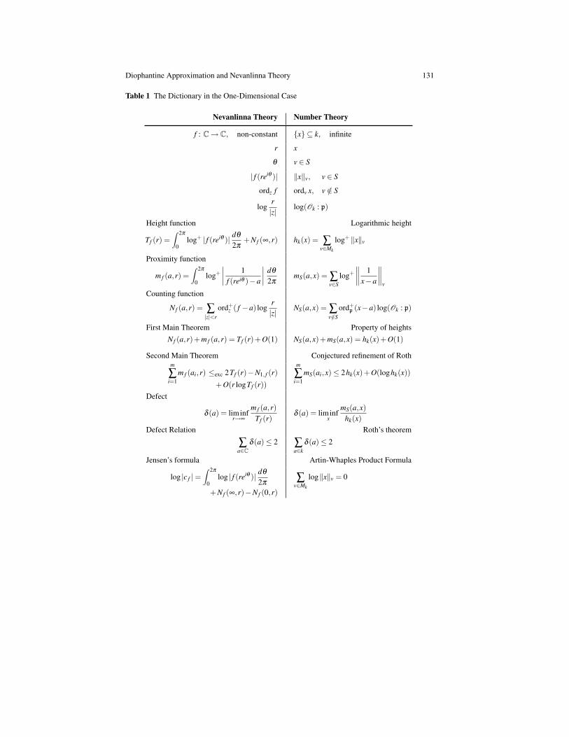
The existence of an analogy between number theory and Nevanlinna theory wasfirst observed by C. F. Osgood [1981, 1985], but he did not provide an explicitdictionary for comparing the two theories. This was provided by Vojta [1987]. Anupdated version of that dictionary is provided here as Table 1.
The first and most important thing to realize about the dictionary is that the ana-logue of a holomorphic (or meromorphic) function is an infinite sequence of rationalnumbers. While it is tempting to compare number theory with Nevanlinna theory byway of function fields—by viewing a single rational point as being analogous to arational point over a function field over C and then applying Nevanlinna theory tothe corresponding section map—this is not what is being compared here. Note thatthe Second Main Theorem posits the non-existence of a meromorphic function vi-olating the inequality for too many r, and Roth’s theorem claims the non-existenceof an infinite sequence of rational numbers not satisfying its main inequality.
We shall now describe Table 1 in more detail. Much of it (below the top six rows)has already been described in Section 5, with the exception of the last line. This isleft to the reader.
The bottom two-thirds of the table can be broken down further, leading to thetop six rows. The first row has been described above. One can say more, though.The analogue of a single rational number can be viewed as the restriction of f tothe closed disc Dr of radius r. Of course f
∣∣Dr
for varying r are strongly related, inthe sense that if one knows one of them then all of them are uniquely determined.This is not true of the number field case (as far as is known); thus the analogy is notperfect.
However, when comparing f∣∣Dr
to a given element of k, there are further similar-ities between the respective proximity functions and counting functions. As far asthe proximity functions are concerned, in Nevanlinna theory m f (a,r) depends onlyon the values of f on the circle |z|= r, whereas in number theory mS(a,r) involvesonly the places in S. So places in S correspond to ∂Dr, and both types of proxim-ity functions involve the absolute values at those places. Moreover, in Nevanlinnatheory the proximity function is an integral over a set of finite measure, while innumber theory the proximity function is a finite sum.
As for counting functions, they involve the open disc Dr in Nevanlinna theory,and places outside of S (all of which are non-archimedean) in number theory. Bothtypes of counting functions involve an infinite weighted sum of orders of vanishingat those places, and the sixth line of Table 1 compares these weights.
Diophantine Approximation and Nevanlinna Theory 131
Table 1 The Dictionary in the One-Dimensional Case
Nevanlinna Theory Number Theory
f : C→ C, non-constant x ⊆ k, infinite
r x
θ v ∈ S
| f (reiθ )| ‖x‖v, v ∈ S
ordz f ordv x, v /∈ S
logr|z|
log(Ok : p)
Height function Logarithmic height
Tf (r) =∫ 2π
0log+ | f (reiθ )| dθ
2π+N f (∞,r) hk(x) = ∑
v∈Mk
log+ ‖x‖v
Proximity function
m f (a,r) =∫ 2π
0log+
∣∣∣∣ 1f (reiθ )−a
∣∣∣∣ dθ
2πmS(a,x) = ∑
v∈Slog+
∥∥∥∥ 1x−a
∥∥∥∥v
Counting function
N f (a,r) = ∑|z|<r
ord+z ( f −a) log
r|z|
NS(a,x) = ∑v/∈S
ord+p (x−a) log(Ok : p)
First Main Theorem Property of heightsN f (a,r)+m f (a,r) = Tf (r)+O(1) NS(a,x)+mS(a,x) = hk(x)+O(1)
Second Main Theorem Conjectured refinement of Rothm
∑i=1
m f (ai,r) ≤exc 2Tf (r)−N1, f (r)
+O(r logTf (r))
m
∑i=1
mS(ai,x)≤ 2hk(x)+O(loghk(x))
Defect
δ (a) = liminfr→∞
m f (a,r)Tf (r)
δ (a) = liminfx
mS(a,x)hk(x)
Defect Relation Roth’s theorem
∑a∈C
δ (a)≤ 2 ∑a∈k
δ (a)≤ 2
Jensen’s formula Artin-Whaples Product Formula
log |c f |=∫ 2π
0log | f (reiθ )| dθ
2π
+N f (∞,r)−N f (0,r)
∑v∈Mk
log‖x‖v = 0
132 Paul Vojta
It should also be mentioned that many of these theorems in Nevanlinna theoryhave been extended to holomorphic functions with domains other than C. In onedirection, one can replace the domain with Cm for some m > 0. While this is usefulfrom the point of view of pure Nevanlinna theory, it is less interesting from the pointof view of the analogy with number theory, since number rings are one-dimensional.Moreover, in Nevanlinna theory, the proofs that correspond most closely to proofsin number theory concern maps with domain C.
There is one other way to change the domain of a holomorphic function, though,which is highly relevant to comparisons with number theory. Namely, one can re-place the domain C with a ramified cover. Let B be a connected Riemann surface, letπ : B→C be a proper surjective holomorphic map, and let f : B→C be a meromor-phic function. In place of Dr in the above discussion, one can work with π−1
(Dr)
and define the proximity, counting, and height functions accordingly. For detaileddefinitions, see Section 26.
When working with a finite ramified covering, though, the Second Main Theoremrequires an additional term NRam(π)(r), which is a counting function for ramifica-tion points of π (Definition 26.3c). The main inequality (4.7.1) of the Second MainTheorem then becomes
q
∑j=1
m f (a j,r)≤exc 2Tf (r)+NRam(π)(r)+O(log+ Tf (r))+o(logr)
in this context.In number theory, the corresponding situation involves algebraic numbers of
bounded degree over k instead of elements of k itself. Again, the inequality in theSecond Main Theorem becomes weaker in this case, conjecturally by adding thefollowing term.
Definition 6.1. Let Dk denote the discriminant of a number field k, and for numberfields L⊇ k define
dk(L) =1
[L : k]log |DL|− log |Dk| .
For x ∈ k we then definedk(x) = dk(k(x)) .
It is then conjectured that Roth’s theorem for x ∈ k of bounded degree over k stillholds, with inequality
(6.2)q
∑j=1
mS(a j,x)≤ (2+ ε)hk(x)+dk(x)+C .
For further discussion of this situation, including its relation to the abc conjecture,see Sections 24–25.
Diophantine Approximation and Nevanlinna Theory 133
7 Cartan’s Theorem and Schmidt’s Subspace Theorem
In both Nevanlinna theory and number theory, the first extensions of the SecondMain Theorem and its counterpart to higher dimensions were theorems involvingapproximation to hyperplanes in projective space.
We start with a definition needed for both theorems.
Definition 7.1. A collection of hyperplanes in Pn is in general position if for allj ≤ n the intersection of any j of them has dimension n− j, and if the intersectionof any n+1 of them is empty.
The Second Main Theorem for approximation to hyperplanes in Pn was firstproved by Cartan [1933]. Before stating it, we need to define the proximity, count-ing, and height functions.
Definition 7.2. Let H be a hyperplane in Pn(C) (n > 0), and let a0x0 + · · ·+ anxnbe a linear form defining it. Let P ∈ Pn \H be a point, and let [x0 : · · · : xn] behomogeneous coordinates for P. We then define
(7.2.1) λH(P) =−12
log|a0x0 + · · ·+anxn|2
|x0|2 + · · ·+ |xn|2
(this depends on a0, . . . ,an, but only up to an additive constant). It is independent ofthe choice of homogeneous coordinates for P.
If n = 1 and H is a finite number a ∈ C (via the usual identification of C as asubset of P1(C)), then
(7.3) λH(x) = log+∣∣∣∣ 1x−a
∣∣∣∣+O(1) .
Recall that a holomorphic curve in a complex variety X is a holomorphic func-tion from C to X(C).
Definition 7.4. Let n, H, and λH be as in Definition 7.2, and let f : C→ Pn be aholomorphic curve whose image is not contained in H. Then the proximity functionfor H is
(7.4.1) m f (H,r) =∫ 2π
0λH( f (reiθ ))
dθ
2π.
For the following, recall that an analytic divisor on C is a formal sum
∑z∈C
nz · z ,
where nz ∈ Z for all z and the set z ∈ C : nz 6= 0 is a discrete set (which may beinfinite).
134 Paul Vojta
Definition 7.5. Let n, H, and f be as above. Then f ∗H is an analytic divisor onC, and for z ∈ C we let ordz f ∗H denote its multiplicity at the point z. Then thecounting function for H is defined to be
(7.5.1) N f (H,r) = ∑0<|z|<r
ordz f ∗H · logr|z|
+ord0 f ∗H · logr
Definition 7.6. Let f : C→ Pn(C) be a holomorphic curve (n > 0). We then definethe height of f to be
Tf (r) = m f (H,r)+N f (H,r)
for any hyperplane H not containing the image of f . The First Main Theorem canbe shown to hold in the context of hyperplanes in projective space, so the heightdepends on H only up to O(1).
We may now state Cartan’s theorem.
Theorem 7.7. (Cartan) Let n > 0 and let H1, . . . ,Hq be hyperplanes in Pn in generalposition. Let f : C→ Pn(C) be a holomorphic curve whose image is not containedin any hyperplane. Then
(7.7.1)q
∑j=1
m f (H j,r)≤exc (n+1)Tf (r)+O(log+ Tf (r))+o(logr) .
If n = 1 then by (7.3) this reduces to the classical Second Main Theorem (Theo-rem 4.7).
Inequality (7.7.1) can also be expressed using counting functions as
(7.8)q
∑j=1
N f (H j,r)≥exc (q−n−1)Tf (r)−O(log+ Tf (r))−o(logr)
(cf. (4.8)).The corresponding definitions and theorem in number theory are as follows.
These will all assume that k is a number field, that S⊇ S∞ is a finite set of places ofk, and that n > 0.
Definition 7.9. Let H be a hyperplane in Pnk and let a0x0 + · · ·+anxn = 0 be a linear
form defining it. (Since Pnk is a scheme over k, this implies that a0, . . . ,an ∈ k.) For
all places v of k and all P ∈ Pn(k) not lying on H we then define
(7.9.1) λH,v(P) =− log‖a0x0 + · · ·+anxn‖v
max‖x0‖v, . . . ,‖xn‖v,
where [x0 : · · · : xn] are homogeneous coordinates for P. Again, this is independentof the choice of homogeneous coordinates [x0 : · · · : xn] and depends on the choiceof a0, . . . ,an only up to a bounded function which is zero for almost all v.
These functions are special cases of Weil functions (Definition 8.6), with domainrestricted to Pn(k)\H.
Diophantine Approximation and Nevanlinna Theory 135
Definition 7.10. For H and P as above, the proximity function for H is defined tobe
(7.10.1) mS(H,P) = ∑v∈S
λH,v(P) ,
and the counting function is defined by
(7.10.2) NS(H,P) = ∑v/∈S
λH,v(P) .
We then note that
mS(H,P)+NS(H,P) = ∑v∈Mk
− log‖a0x0 + · · ·+anxn‖v
max‖x0‖v, . . . ,‖xn‖v
= ∑v∈Mk
logmax‖x0‖v, . . . ,‖xn‖v
= hk(P)
by the Product Formula.Although this equality holds exactly, the proximity and counting functions de-
pend (up to O(1)) on the choice of linear form a0x0 + · · ·+anxn describing D, so weregard them as being defined only up to O(1).
The counterpart to Theorem 7.7 (with, of course, a weaker error term) is a slightlyweaker form of Schmidt’s Subspace Theorem.
Theorem 7.11. (Schmidt) Let k, S, and n be as above, let H1, . . . ,Hq be hyperplanesin Pn
k in general position, let ε > 0, and let c ∈ R. Then
(7.11.1)q
∑j=1
mS(H j,x)≤ (n+1+ ε)hk(x)+ c
for all x∈Pn(k) outside of a finite union of proper linear subspaces of Pnk . This latter
set depends on k, S, H1, . . . ,Hq, ε , c, and the choices used in defining the mS(H j,x),but not on x.
When n = 1 this reduces to Roth’s theorem (in the form of Theorem 3.5).Note, in particular, that the Hi are hyperplanes in the k-scheme Pn
k . This automat-ically implies that they can be defined by linear forms with coefficients in k. Thiscorresponds to requiring the α j to lie in k in the case of Roth’s theorem. Schmidt’soriginal formulation of his theorem allowed hyperplanes with algebraic coefficients;the reduction to hyperplanes in Pn
k is similar to the reduction for Roth’s theorem andis omitted here. Also, Schmidt’s original formulation was stated in terms of hyper-planes in An+1
k passing through the origin and points in An+1k with integral coeffi-
cients. He also used the size instead of the height. For details on the equivalence ofhis original formulation and the form given here, see [Vojta, 1987, Ch. 2 § 2].
136 Paul Vojta
Theorem 7.11 is described as a slight weakening of Schmidt’s Subspace Theorembecause Schmidt actually allowed the set of hyperplanes to vary with v. Thus, to geta statement that was fully equivalent to Schmidt’s original theorem, (7.11.1) wouldneed to be replaced by
∑v∈S
qv
∑j=1
mS(Hv, j,x)≤ (n+1+ ε)hk(x)+ c ,
where for each v ∈ S, Hv,1, . . . ,Hv,qv are hyperplanes in general position (but in to-tality the set Hv, j : v ∈ S, 1 ≤ j ≤ qv need not be in general position, even aftereliminating duplicates). Of course, at a given place v a point can be close to at mostn of the Hv, j, so we may assume qv = n for all v (or actually n+1 is somewhat easierto work with).
Thus, a full statement of Schmidt’s Subspace Theorem, rendered using the nota-tion of Section 5, is as follows. It has been stated in a form that most readily carriesover to Nevanlinna theory.
Theorem 7.12. (Schmidt’s Subspace Theorem [Schmidt, 1991, Ch. VIII, Thm. 7A])Let k, S, and n be as above, and let H1, . . . ,Hq be distinct hyperplanes in Pn
k . Thenfor all ε > 0 and all c ∈ R the inequality
(7.12.1) ∑v∈S
maxJ
∑j∈J
λH j ,v(x)≤ (n+1+ ε)hk(x)+ c
holds for all x∈Pn(k) outside of a finite union of proper linear subspaces dependingonly on k, S, H1, . . . ,Hq, ε , c, and the choices used in defining the λH j ,v. The max inthis inequality is taken over all subsets J of 1, . . . ,q corresponding to subsets ofH1, . . . ,Hq in general position.
In Nevanlinna theory there are infinitely many angles θ , so if one allowed thecollection of hyperplanes to vary with θ without additional restriction, then the re-sulting statement could involve infinitely many hyperplanes, and would thereforelikely be false (although this has not been proved). Therefore an overall restrictionon the set of hyperplanes is needed in the case of Cartan’s theorem, and is whyTheorem 7.12 was stated in the way that it was.
Cartan’s theorem itself can be generalized as follows.
Theorem 7.13. [Vojta, 1997] Let n ∈ Z>0, let H1, . . . ,Hq be hyperplanes in PnC, and
let f : C→ Pn(C) be a holomorphic curve whose image is not contained in a hy-perplane. Then∫ 2π
0max
J∑j∈J
λH j( f (reiθ ))dθ
2π≤exc (n+1)Tf (r)+O(log+ Tf (r))+o(logr) ,
where J varies over the same collection of sets as in Theorem 7.12.
This has proved to be a useful formulation for applications; see [Vojta, 1997] and[Ru, 1997]. The latter reference also improves the error term in Theorem 7.13.
Diophantine Approximation and Nevanlinna Theory 137
Remark 7.14. It has been further shown that in Theorem 7.12, the finite set of lin-ear subspaces can be taken to be the union of a finite number of points (dependingon the same data as given in the theorem), together with a finite union of linearsubspaces (of higher dimension) depending only on the collection of hyperplanes[Vojta, 1989]. In other words, the higher-dimensional part of the exceptional setdepends only on the geometric data. Correspondingly, Theorem 7.13 holds for allnonconstant holomorphic curves whose image is not contained in the union of thislatter set [Vojta, 1997]. For an example of the collection of higher dimensional sub-spaces for a specific set of lines in P2, see Example 13.3.
8 Varieties and Weil Functions
The goal of this section and the next is to carry over the definitions of the proximity,counting, and height functions to the context of varieties.
First it is necessary to define variety. Generally speaking, varieties and otheralgebro-geometric objects are as defined in [Hartshorne, 1977], except that varieties(when discussing number theory at least) may be defined over a field that is notnecessarily algebraically closed.
Definition 8.1. A variety over a field k, or a k-variety, is an integral separatedscheme of finite type over k (i.e., over Speck). A curve over k is a variety overk of dimension 1. A morphism of varieties over k is a morphism of k-schemes.Finally, a subvariety of a variety (resp. closed subvariety, open subvariety) is anintegral subscheme (resp. closed integral subscheme, open integral subscheme) ofthat variety (with induced map to Speck).
As an example, X := SpecQ[x,y]/(y2−2x2) is a variety over Q. Indeed, it is anintegral scheme because the ring Q[x,y]/(y2−2x2) is entire. However, X×Q Q
(√2)
is not a variety over Q(√
2), since Q[x,y]/(y2− 2x2)⊗Q Q
(√2)
is not entire (thepolynomial y2− 2x2 is not irreducible over Q
(√2)). Therefore, some authors re-
quire a variety to be geometrically integral, but we do not do so here. The advantageof not requiring geometric integrality is that every reduced closed subset is a finiteunion of closed subvarieties, without requiring base change to a larger field.
Many people would be tempted to say that the variety X := SpecQ[x,y]/(y2−2x2)is not defined over Q. Such wording does not make sense in this context (the varietyis, after all, a Q-variety). This wording usually comes about because the variety (inthis instance) is associated to the line y =
√2x in A2
Q, which does not come from
any subvariety of A2Q (without also obtaining the conjugate y =−
√2x). The correct
way to express this situation is to say that X is not geometrically irreducible (or notgeometrically integral).
Strictly speaking, if k ⊆ L are distinct fields, then X(k) and X(L) are disjointsets. However, we will at times identify X(k) with a subset of X(L) in the obviousway. Following EGA, if x ∈ X is a point, then κ(x) will denote the residue field of
138 Paul Vojta
the local ring at x. If x ∈ X(L), then it is technically a morphism, but by abuse ofnotation κ(x) will refer to the corresponding point on X (so κ(x) may be smallerthan L).
We also recall that the function field of a variety X is denoted K(X). If ξ is thegeneric point of X , then K(X) = κ(ξ ).
The next goal of this section is to introduce Weil functions. These functions wereintroduced in Weil’s thesis [Weil, 1928] and further developed in a later paper [Weil,1951]. Weil functions give a way to write the height as a sum over places of anumber field, and are exactly what is needed in order to generalize the proximityand counting functions to the geometric setting.
The description provided here will be somewhat brief; for a fuller treatment, see[Lang, 1983, Ch. 10].
We start with the very easy setting used in Nevanlinna theory.Weil functions are best described using Cartier divisors.
Definition 8.2. Let D be a Cartier divisor on a complex variety X . Then a Weil func-tion for D is a function λD : (X \SuppD)(C)→R such that for all x ∈ X there is anopen neighborhood U of x in X , a nonzero function f ∈ K(X) such that D
∣∣U = ( f ),
and a continuous function α : U(C)→ R such that
(8.2.1) λD(x) =− log | f (x)|+α(x)
for all x ∈ (U \SuppD)(C). Here the topology on U(C) is the complex topology.
It is fairly easy to show that if λD is a Weil function, then the above condition issatisfied for any open set U and any nonzero f ∈ OU satisfying D
∣∣U = ( f ).
Recall that linear equivalence classes of Cartier divisors on a variety are in natu-ral one-to-one correspondence with isomorphism classes of line sheaves (invertiblesheaves) on that variety. Moreover, for each divisor D on a variety X , if L is thecorresponding line sheaf, then there is a nonzero rational section s of L whose van-ishing describes D: D = (s). As was noted by Neron, Weil functions on D correspondto metrics on L .
Recall that if X is a complex variety and L is a line sheaf on X , then a metric onL is a collection of norms on the fibers of the complex line bundle corresponding tothe sheaf L , varying smoothly or continuously with the point on X . Such a metric iscalled a smooth metric or continuous metric, respectively. In these notes, smoothmeans C∞. If X is singular, then we say that a function f : X(C)→C is C∞ at a pointP∈ X(C) if there is an open neighborhood U of P in X(C) in the complex topology,a holomorphic function φ : U →Cn for some n, and a C∞ function g : Cn→C suchthat f = gφ . This reduces to the usual concept of C∞ function at smooth points ofX .
To describe a metric on L in concrete terms, let U be an open subset of X and letφU : OU
∼→L∣∣U be a local trivialization. Then the function ρU : U(C)→R>0 given
by ρU (x) = |φU (1)(x)| is smooth (resp. continuous), and for any section s ∈L (U)and any x ∈U(C), we have |s(x)| = ρU (x) · |φ−1
U (s)(x)|. Moreover, if V is another
Diophantine Approximation and Nevanlinna Theory 139
open set in X and φV : OV∼→L
∣∣V is a local trivialization on V , then φ
−1U φV (ap-
propriately restricted) is an automorphism of OU∩V corresponding to multiplicationby a function αUV ∈ O∗U∩V . Again letting ρV (x) = |φV (1)(x)|, we see that ρU andρV are related by ρV (x) = |αUV (x)|ρU (x) for all x ∈ (U ∩V )(C).
Conversely, an isomorphism class of line sheaves on X can be uniquely specifiedby giving an open cover U of X and αUV ∈ O∗U∩V for all U,V ∈ U satisfyingαUU = 1 and αUW = αUV αVW on U ∩V ∩W for all U,V,W ∈ U . Moreover, withthese data, one can specify a metric on the associated line sheaf by giving smooth orcontinuous functions ρU : U(C)→ R>0 for each U ∈U that satisfy ρV = |αUV |ρUon U ∩V for all U,V ∈U .
A continuous metric on a line sheaf L determines a Weil function for any as-sociated Cartier divisor D. Indeed, if s is a nonzero rational section of L such thatD = (s), then λD(x) =− log |s(x)| is a Weil function for D. Conversely, a Weil func-tion for D determines a continuous metric on L .
In Nevanlinna theory it is customary to work only with smooth metrics, andhence it is often better to work with Weil functions associated to smooth metrics(equivalently, to Weil functions for which the functions α in (8.2.1) are all smooth).
An example of a Weil function in Nevanlinna theory (and perhaps the primaryexample) is the function λH of Definition 7.2 used in Cartan’s theorem.
Likewise, the function λH,v of Definition 7.9 is an example of a Weil function innumber theory. In this case, it is no longer sufficient to say that two Weil functionsagree up to O(1): the implied constant also has to vanish for almost all v. For exam-ple, Lemma 5.4 compares the difference of two Weil functions, and shows that thedifference is bounded by a bound that vanishes for almost all v. A plain bound ofO(1) would not suffice to give a finite bound in Theorem 5.5.
Before defining Weil functions in the number theory case, we first give somedefinitions relevant to the domains of Weil functions.
Definition 8.3. Let v be a place of a number field k. Then Cv is the completion ofthe algebraic closure kv of the completion kv of k at v.
Recall [Koblitz, 1984, Ch. III, § 3–4] that if v is non-archimedean then kv is notcomplete, but its completion Cv is algebraically closed. If v is archimedean, thenCv is isomorphic to the field of complex numbers (as is kv). The norm ‖ · ‖v on kextends uniquely to norms on kv, on kv, and on Cv. If X is a variety, then the normon Cv defines a topology on X(Cv), called the v-topology. It is defined to be thecoarsest topology such that for all open U ⊆ X and all f ∈ O(U), U(Cv) is openand f : U(Cv)→ Cv is continuous.
One can also work just with the algebraic closure kv when defining Weil func-tions, without any essential difference.
Definition 8.4. Let X be a variety over a number field k. Then X(Mk) is the disjointunion
X(Mk) =∐
v∈Mk
X(Cv) .
This set is given a topology defined by the condition that A⊆ X(Mk) is open if andonly if A∩X(Cv) is open in the v-topology for all v.
140 Paul Vojta
Definition 8.5. Let k be a number field. Then an Mk-constant is a collection (cv) ofconstants cv ∈ R for each v ∈Mk, such that cv = 0 for almost all v. If X is a varietyover k, then a function α : X(Mk)→R is said to be OMk(1) if there is an Mk-constant(cv) such that |α(x)| ≤ cv for all x ∈ X(Cv) and all v ∈Mk.
We may then define Weil functions as follows.
Definition 8.6. Let X be a variety over a number field k, and let D be a Cartierdivisor on X . Then a Weil function for D is a function λD : (X \SuppD)(Mk)→ Rthat satisfies the following condition. For each x ∈ X there is an open neighborhoodU of x, a nonzero function f ∈O(U) such that D
∣∣U = ( f ), and a continuous locally
Mk-bounded function α : U(Mk)→ R satisfying
(8.6.1) λD(x) =− log‖ f (x)‖v +α(x)
for all v ∈Mk and all x ∈ (U \SuppD)(Cv).
For the definition of locally Mk-bounded function, see [Lang, 1983, Ch. 10, § 1].The definition is more complicated than one would naively expect, stemming fromthe fact that Cv is totally disconnected, and not locally compact. For our purposes,though, it suffices to note that if X is a complete variety then such a function isOMk(1). (In other contexts, these problems are dealt with by using Berkovich spaces,but Weil’s work does not use them, not least because it came much earlier.)
As with Definition 8.2, if λ is a Weil function for D, then it can be shown that theabove condition is true for all open U ⊆ X and all f ∈ O(U) for which D
∣∣U = ( f ).
If λD is a Weil function for D, then we write
λD,v = λD∣∣(X\SuppD)(Cv)
for all places v of k. If v is an archimedean place, then Cv ∼= C, and λD,v is a Weilfunction for D in the sense of Definition 8.2 (up to a factor 1/2 if v is a complexplace).
In the future, if x ∈ X(Mk) and f is a function on X , then ‖ f (x)‖ will mean‖ f (x)‖v for the (unique) place v such that x ∈ X(Cv). Thus, (8.6.1) could be short-ened to λ (x) =− log‖ f (x)‖+α(x) for all x ∈ (U \SuppD)(Mk).
Of course, this discussion would be academic without the following theorem.
Theorem 8.7. Let k be a number field, let X be a projective variety over k, and letD be a Cartier divisor on X. Then there exists a Weil function for D.
For the proof, see [Lang, 1983, Ch. 10]. This is also true for complete vari-eties, using Nagata’s embedding theorem to construct a model for X and then usingArakelov theory to define the Weil function. But, again, the details are beyond thescope of these notes.
Weil functions have the following properties.
Theorem 8.8. Let X be a complete variety over a number field k. Then
Diophantine Approximation and Nevanlinna Theory 141
(a). Additivity: If λ1 and λ2 are Weil functions for Cartier divisors D1 and D2 onX, respectively, then λ1 +λ2 extends uniquely to a Weil function for D1 +D2.
(b). Functoriality: If λ is a Weil function for a Cartier divisor D on X, andif f : X ′ → X is a morphism of k-varieties such that f (X ′) * SuppD, thenx 7→ λ ( f (x)) is a Weil function for the Cartier divisor f ∗D on X ′.
(c). Normalization: If X = Pnk , and if D is the hyperplane at infinity, then the
function
(8.8.1) λD,v([x0 : · · · : xn]) :=− log‖x0‖v
max‖x0‖v, . . . ,‖xn‖v
is a Weil function for D.(d). Uniqueness: If both λ1 and λ2 are Weil functions for a Cartier divisor D on
X, then λ1 = λ2 +OMk(1).(e). Boundedness from below: If D is an effective Cartier divisor and λ is a Weil
function for D, then λ is bounded from below by an Mk-constant.(f). Principal divisors: If D is a principal divisor ( f ), then − log‖ f‖ is a Weil
function for D.
The proofs of these properties are left to the reader (modulo the properties oflocally Mk-bounded functions).
Parts (b) and (c) of the above theorem combine to give a way of computing Weilfunctions for effective very ample divisors. This, in turn, gives rise to the “max-min”method for computing Weil functions for arbitrary Cartier divisors on projectivevarieties.
Lemma 8.9. Let λ1, . . . ,λn be Weil functions for Cartier divisors D1, . . . ,Dn, respec-tively, on a complete variety X over a number field k. Assume that the divisors Diare of the form Di = D0 +Ei, where D0 is a fixed Cartier divisor and Ei are effectivefor all i. Assume also that SuppE1∩·· ·∩SuppEn = /0. Then the function
λ (x) = minλi(x) : x /∈ SuppEi
is defined everywhere on (X \SuppD0)(Mk), and is a Weil function for D0.
Proof. See [Lang, 1983, Ch. 10, Prop. 3.2]. ut
Theorem 8.10. (Max-min) Let X be a projective variety over a number field k, andlet D be a Cartier divisor on X. Then there are positive integers m and n, andnonzero rational functions fi j on X, 1 = 1, . . . ,n, j = 1, . . . ,m, such that
λ (x) := max1≤i≤n
min1≤ j≤m
(− log‖ fi j‖
)defines a Weil function for D.
Proof. We may write D as a difference E−F of very ample divisors. Let E1, . . . ,Enbe effective Cartier divisors linearly equivalent to E such that
⋂SuppEi = /0 (for
142 Paul Vojta
example, pull-backs of hyperplane sections via a projective embedding associatedto E). Likewise, let F1, . . . ,Fm be effective Cartier divisors linearly equivalent to Fwith
⋂SuppFj = /0. Then D−Ei +Fj is a principal divisor for all i and j; hence
D−Ei +Fj = ( fi j)
for some fi j ∈ K(X)∗ and all i and j. Applying Lemma 8.9 to − log‖ fi j‖ then im-plies that min1≤ j≤m
(− log‖ fi j‖
)is a Weil function for D−Ei for all i. Applying
Lemma 8.9 again to the negatives of these Weil functions then gives the theorem.ut
To conclude the section, we give some notation that will be useful for workingwith rational and algebraic points.
Definition 8.11. Let X be a variety over a number field k, let D be a Cartier divisoron X , and let λD be a Weil function for D. If L is a number field containing k, andif w is a place of L lying over a place v of k, then we identify Cw with Cv in theobvious manner, and write
(8.11.1) λD,w = [Lw : kv]λD,v .
(Recall that ‖x‖w = ‖x‖[Lw:kv]v for all x ∈ Cv, by (1.4).) Finally, each point x ∈ X(L)
gives rise to points xw ∈ X(Cw) for all w ∈ML, and we define
(8.11.2) λD,w(x) = λD,w(xw)
if x /∈ SuppD.
Note that, if x ∈ (X \SuppD)(L), if L′ is a number field containing L, if w is aplace of L, and if w′ is a place of L′ lying over w, then
(8.12) λD,w′(x) = [L′w′ : Lw]λD,w(x) ,
regardless of whether the left-hand side is defined using (8.11.1) or (8.11.2) (byregarding X(L) as a subset of X(L′) for the latter).
If (cv) is an Mk-constant, if w is a place of a number field L containing k, and ifv is the place of k lying under w, then we write
(8.13) cw = [Lw : kv]cv ,
so that the condition λD,w ≤ cw will be equivalent to λD,v ≤ cv, by (8.11.1).
Diophantine Approximation and Nevanlinna Theory 143
9 Height Functions on Varieties in Number Theory
Weil functions can be used to generalize the height hk (defined in Section 2) toarbitrary complete varieties over k. This can also be done by working directly withheights; see [Lang, 1983, Ch. 3] or [Silverman, 1986].
Throughout this section, k is a number field, X is a complete variety over k,and D is a Cartier divisor on X , unless otherwise specified.
Definition 9.1. Let λ be a Weil function for D, and let x ∈ X(k) be an algebraicpoint with x /∈ SuppD. Then the height of x relative to λ and k is defined as
(9.1.1) hλ ,k(x) =1
[L : k] ∑w∈ML
λw(x)
for any number field L⊇ κ(x). It is independent of the choice of L by (8.12).
In particular, if x ∈ X(k), then
hλ ,k(x) = ∑v∈Mk
λv(x) .
Specializing in a different direction, if X = Pnk , if D is the hyperplane at infinity,
and if λ is the Weil function (8.8.1), then
hλ ,k([x0 : · · · : xn]) =− 1[L : k] ∑
w∈ML
log‖x0‖v
max‖x0‖v, . . . ,‖xn‖v
=1
[L : k] ∑w∈ML
logmax‖x0‖v, . . . ,‖xn‖v
= hk([x0 : · · · : xn])
(9.2)
for all [x0 : · · · : xn] ∈ Pn(k) with x0 6= 0, where L is any number field containing thefield of definition of this point.
The restriction x /∈ SuppD can be eliminated as follows.Let D′ be another Cartier divisor on X linearly equivalent to D, say D′ = D+( f );
then λ ′ := λ − log‖ f‖ is a Weil function for D′. If x ∈ X(k) does not lie onSuppD∪SuppD′, and if L is a number field containing κ(x), then
hλ ′,k(x) =1
[L : k] ∑w∈ML
λ′v(x)
=1
[L : k] ∑w∈ML
λv(x)−1
[L : k] ∑w∈ML
log‖ f (x)‖w
= hλ ,k(x)
(9.3)
144 Paul Vojta
by the Product Formula (1.6). Thus we have:
Definition 9.4. Let λ be a Weil function for D, and let x ∈ X(k). Then, for anyf ∈ K(X)∗ such that the support of D+( f ) does not contain x, we define
hλ ,k(x) = hλ−log‖ f‖,k(x) ,
where hλ−log‖ f‖,k on the right-hand side is defined using Definition 9.1. This ex-pression is independent of the choice of f by (9.3), and agrees with Definition 9.1when x /∈ SuppD since we can take f = 1 in that case.
With this definition, (9.2) holds without the restriction x0 6= 0.
Proposition 9.5. If both λ and λ ′ are Weil functions for D, then
hλ ′,k = hλ ,k +O(1) .
Proof. Indeed, this is immediate from Theorem 8.8d. ut
Thus, the height function defined above depends only on the divisor; moreover,by (9.3) it depends only on the linear equivalence class of the divisor.
Definition 9.6. The height hD,k(x) for points x ∈ X(k) is defined, up to O(1), as
hD,k(x) = hλ ,k(x)
for any Weil function λ for D. If L is a line sheaf on X , then we define
hL ,k(x) = hD,k(x)
for points x ∈ X(k), where D is any Cartier divisor for which O(D)∼= L . Again, itis only defined up to O(1).
By (9.2), we then havehO(1),k = hk +O(1)
on Pnk for all n > 0. Since the automorphism group of Pn
k is transitive on the set of ra-tional points, and since automorphisms preserve the line sheaf O(1), the term O(1)in the above formula cannot be eliminated without additional structure. Thus, Defi-nition 9.6 cannot give an exact definition for the height without additional structure.(This additional structure can be given using Arakelov theory.)
Theorem 8.8 and (8.12) also immediately imply the following properties ofheights:
Theorem 9.7. (a). Functoriality: if f : X ′→ X is a morphism of k-varieties, andif L is a line sheaf on X, then
h f ∗L ,k(x) = hL ,k( f (x))+O(1)
for all x ∈ X ′(k), where the implied constant depends only on f , L , and thechoices of the height functions.
Diophantine Approximation and Nevanlinna Theory 145
(b). Additivity: if L1 and L2 are line sheaves on X, then
hL1⊗L2,k(x) = hL1,k(x)+hL2,k(x)+O(1)
for all x∈ X(k), where the implied constant depends only on L1, L2, and thechoices of the height functions.
(c). Base locus: If hD,k is a height function for D, then it is bounded from belowoutside of the base locus of the complete linear system |D|.
(d). Globally generated line sheaves: If L is a line sheaf on X, and is generatedby its global sections, then hL ,k(x) is bounded from below for all x ∈ X(k),by a bound depending only on L and the choice of height function.
(e). Change of number field: If L⊇ k then
hL ,L(x) = [L : k]hL ,k(x)
for all line sheaves L on X and all x∈ X(k). (Strictly speaking, the left-handside should be hL ′,L(x′), where L ′ is the pull-back of L to XL := X×k L andx′ is the point in XL(k) corresponding to x ∈ X(k).)
Corollary 9.8. If L is an ample line sheaf on X, then hL ,k(x) is bounded frombelow for all x ∈ X(k), by a bound depending only on L and the choice of heightfunction.
Proof. By Theorem 9.7b, we may replace L with L ⊗n for any positive integern, and therefore may assume that L is very ample. Then the result follows fromTheorem 9.7d. ut
The following result shows that heights relative to ample line sheaves are thelargest possible heights, up to a constant multiple.
Proposition 9.9. Let L and M be line sheaves on X, with L ample. Then there isa constant C, depending only on L and M , such that
hM ,k(x)≤C hL ,k(x)+O(1)
for all x∈X(k), where the implied constant depends only on L , M , and the choicesof height functions.
Proof. By the definition of ampleness, there is an integer n such that the line sheafL ⊗n⊗M ∨ is generated by global sections. Therefore an associated height function
hL⊗n⊗M∨,k = nhL ,k−hM ,k +O(1)
is bounded from below, giving the result with C = n. ut
For projective varieties, Northcott’s finiteness theorem can be carried over.
Theorem 9.10. (Northcott) Assume that X is projective, and let L be an ample linesheaf on X. Then, for all integers d and all c ∈ R, the set
146 Paul Vojta
(9.10.1) x ∈ X(k) : [κ(x) : k]≤ d and hL ,k(x)≤ c
is finite.
Proof. First, if X = Pnk and L = O(1), then the result follows by bounding the
heights of [xi : x0] (if x0 6= 0, which we assume without loss of generality), andapplying Theorem 2.7 to these points for each i. The general case then follows byreplacing L with a very ample positive multiple and using an associated projectiveembedding and functoriality of heights. ut
Of course, if X is not projective then it has no ample divisors, making the abovetwo statements vacuous. Complete varieties have a notion that is almost as good,though.
Definition 9.11. Let X be a complete variety over an arbitrary field. A line sheaf Lon X is big if there is a constant c > 0 such that
h0(X ,L ⊗n)≥ cndimX
for all sufficiently large and divisible n. A Cartier divisor D on X is big if O(D) isbig.
If X is a complete variety over an arbitrary field, then by Chow’s lemma there isa projective variety X ′ and a proper birational morphism π : X ′→ X . If L is a bigline sheaf on X , then π∗L is big on X ′. Therefore, it makes some sense to comparebig line sheaves with ample ones.
Proposition 9.12. (Kodaira’s lemma) Let X be a projective variety over an arbitraryfield, and let L and A be line sheaves on X, with A ample. Then L is big if andonly if there is a positive integer n such that H0(X ,L ⊗n⊗A ∨) 6= 0. Equivalently,if D and A are Cartier divisors on X, with A ample, then D is big if and only if somepositive multiple of it is linearly equivalent to the sum of A and an effective divisor.
Proof. See [Vojta, 1987, Prop. 1.2.7]. ut
The above allows us to show that heights relative to big line sheaves are also,well, big.
Proposition 9.13. Let X be a complete variety over a number field. Let L and Mbe line sheaves on X, with L big. Then there is a constant C and a proper Zariski-closed subset Z of X, depending only on L and M , such that
hM ,k(x)≤C hL ,k(x)+O(1)
for all x ∈ X(k) outside of Z, where the implied constant depends only on L , M ,and the choices of height functions.
Diophantine Approximation and Nevanlinna Theory 147
Proof. After applying Chow’s lemma and pulling back L and M , we may assumethat X is projective. We may also replace L with a positive multiple, and hence mayassume that L is isomorphic to A ⊗O(D), where A is an ample line sheaf andD is an effective Cartier divisor. Then the result follows from Proposition 9.9, withZ = SuppD, by Theorem 9.7. ut
Unfortunately, it is still not true that an arbitrary complete variety must have abig line sheaf. But it is true if the variety is nonsingular, since one can then take thecomplement of any open affine subset.
For general complete varieties, we can do the following.
Remark 9.14. For a general complete variety X over k, we can define a big heightto be a function h : X(k)→ R for which there exist disjoint subvarieties U1, . . . ,Unof X (not necessarily open or closed), with
⋃Ui = X ; and for each i = 1, . . . ,n a
projective embedding Ui → U i, an ample line sheaf Li on U i, and real constantsci > 0 and Ci such that h(x)≥ ci hLi,k(x)+Ci for all x ∈Ui(k). One can then show:
• every complete variety over k has a big height;• any two big heights on a given complete variety are bounded from above by
linear functions of each other;• if X is a projective variety and L is an ample line sheaf on X then hL ,k is a big
height on X ;• if L is a line sheaf on X then there are real constants c and C such that
hL ,k(x)≤ ch(x)+C for all x ∈ X(k);• the restriction of a big height to a closed subvariety is a big height on that subva-
riety; and• a counterpart to Proposition 9.15 (below) holds for big heights on complete vari-
eties.
Details of these assertions are left to the reader.Big heights are useful for error terms: the conjectures and theorems that follow
are generally stated for projective varieties, with an error term involving a heightrelative to an ample divisor. However, they can also be stated more generally forcomplete varieties if the height is changed to a big height. For concreteness, though,the more restricted setting of projective varieties is used.
Finally, we note a case in which Z can be bounded explicitly. This will be usedin the proof of Proposition 29.3.
Proposition 9.15. Let f : X1→X2 be a morphism of projective varieties over a num-ber field, and let A1 and A2 be ample line sheaves on X1 and X2, respectively. Thenthere is a constant C, depending only on f , A1, and A2 such that
(9.15.1) hA1,k(x)≤C hA2,k( f (x))+O(1)
for all points x ∈ X1(k) that are isolated in their fibers of f , where the impliedconstant depends only on f , A1, A2, and the choices of height functions.
148 Paul Vojta
Proof. If no closed points x of X1 are isolated in their fibers of f , then there isnothing to prove. If there is at least one such point x, then dim f (X1) = dimX1, sof ∗A2 is big. The result then follows by Proposition 9.13 and noetherian inductionapplied to the irreducible components of the set Z in that proposition ut
Note that if any fiber component of f has dimension > 0, then it contains alge-braic points of arbitrarily large height, so (9.15.1) cannot possibly hold for all suchpoints.
10 Proximity and Counting Functions on Varieties in NumberTheory
The definitions of proximity and counting functions given in Sections 5 and 7 alsogeneralize readily to points on varieties.
Throughout this section, k is a number field, S is a finite set of places of kcontaining S∞, and X is a complete variety over k.
Definition 10.1. Let D be a Cartier divisor on X , let λD be a Weil function for D, letx ∈ X(k) with x /∈ SuppD, let L ⊇ k be a number field such that x ∈ X(L), and letT be the set of places of L lying over places in S. Then the proximity function andcounting function in this setting are defined up to O(1) by
mS(D,x) =1
[L : k] ∑w∈T
λD,w(x) and NS(D,x) =1
[L : k] ∑w/∈T
λD,w(x) .
These expressions are independent of the choice of L, by (8.11.1). They depend onthe choice of λD only up to O(1).
Unlike the height, the proximity and counting functions depend on D, even withina linear equivalence class. Therefore the restriction x /∈ SuppD cannot be eliminated.
By (9.1.1) and Definition 9.6, we have
hD,k(x) = mS(D,x)+NS(D,x)
for all x ∈ X(k) outside of the support of D. This is, basically, the First Main The-orem. The Second Main Theorem in this context is still a conjecture (Conjecture14.6).
Theorem 8.8 immediately implies the following properties of proximity andcounting functions.
Proposition 10.2. In number theory, proximity and counting functions have the fol-lowing properties.
Diophantine Approximation and Nevanlinna Theory 149
(a). Additivity: If D1 and D2 are Cartier divisors on X, then
mS(D1 +D2,x) = mS(D1,x)+mS(D2,x)+O(1)
and
NS(D1 +D2,x) = NS(D1,x)+NS(D2,x)+O(1)
for all x ∈ X(k) outside of the supports of D1 and D2.(b). Functoriality: If f : X ′→ X is a morphism of complete k-varieties and D is
a divisor on X whose support does not contain the image of f , then
mS( f ∗D,x) = mS(D, f (x))+O(1)
and
NS( f ∗D,x) = NS(D, f (x))+O(1)
for all x ∈ X ′(k) outside of the support of f ∗D.(c). Effective divisors: If D is an effective Cartier divisor on X, then mS(D,x) and
NS(D,x) are bounded from below for all x ∈ X(k) outside of the support ofD.
(d). Change of number field: If L is a number field containing k and if T is theset of places of L lying over places in S, then
mT (D,x) = [L : k]mS(D,x)+O(1)
and
NT (D,x) = [L : k]NS(D,x)+O(1)
for all x ∈ X(k) outside of the support of D (with the same abuse of notationas in Theorem 9.7e).
In each of the above cases, the implied constant in O(1) depends on the varieties,divisors, and morphisms, but not on x.
When working with proximity and height functions, the divisor D is almost al-ways assumed to be effective.
11 Height, Proximity, and Counting Functions in NevanlinnaTheory
The height, proximity, and counting functions of Nevanlinna theory can also begeneralized to the context of a divisor on a complete complex variety.
150 Paul Vojta
In this section, X is a complete complex variety, D is a Cartier divisor onX , and f : C→ X is a holomorphic curve whose image is not contained inthe support of D. Throughout these notes, we will often implicitly think of acomplex variety X as a complex analytic space [Hartshorne, 1977, App. B].
We begin with the proximity and counting functions.
Definition 11.1. Let λ be a Weil function for D. Then the proximity function for frelative to D is the function
m f (D,r) =∫ 2π
0λ ( f (reiθ ))
dθ
2π.
It is defined only up to O(1).
If λ ′ is another Weil function for D, then |λ −λ ′| is bounded, so the proximityfunction is independent of D (up to O(1)).
Definition 11.2. The counting function for f relative to D is the function
N f (D,r) = ∑0<|z|<r
ordz f ∗D · logr|z|
+ord0 f ∗D · logr .
Unlike the proximity function and the counting function in Nevanlinna theory,this function is defined exactly.
Corresponding to Proposition 10.2, we then have
Proposition 11.3. In Nevanlinna theory, proximity and counting functions have thefollowing properties.
(a). Additivity: If D1 and D2 are Cartier divisors on X, then
m f (D1 +D2,r) = m f (D1,r)+m f (D2,r)+O(1)
and
N f (D1 +D2,r) = N f (D1,r)+N f (D2,r) .
(b). Functoriality: If φ : X → X ′ is a morphism of complete complex varietiesand D′ is a Cartier divisor on X ′ whose support does not contain the imageof φ f , then
m f (φ ∗D′,r) = mφ f (D′,r)+O(1) and N f (φ ∗D′,r) = Nφ f (D′,r) .
(c). Effective divisors: If D is effective, then m f (D,r) is bounded from below andN f (D,r) is nonnegative.
Diophantine Approximation and Nevanlinna Theory 151
In each of the above cases, the implied constant in O(1) depends on the varieties,divisors, and morphisms, but not on f or r.
We can now define the height.
Definition 11.4. The height function relative to D is defined, up to O(1), as
TD, f (r) = m f (D,r)+N f (D,r) .
Proposition 11.5. The height function TD, f is additive in D, is functorial, and isbounded from below if D is effective, as in Proposition 11.3.
Proof. Immediate from Proposition 11.3. ut
Proposition 11.6. (First Main Theorem) Let D′ be another Cartier divisor on Xwhose support does not contain the image of f , and assume that D′ is linearly equiv-alent to D. Then
(11.6.1) TD′, f (r) = TD, f (r)+O(1) .
Proof. We first consider the special case X = P1C, D = [0] (the image of the
point 0 under the injection A1 → P1), and D′ = [∞] (the point at infinity, withmultiplicity one). Then TD′, f (r) = Tf (r) + O(1), m f (D,r) = m f (0,r) + O(1), andN f (D,r) = N f (0,r) (where Tf (r), m f (0,r), and N f (0,r) are as defined in Section4). The result then follows by Theorem 4.6 (the First Main Theorem for meromor-phic functions).
In the general case, write D−D′ = (g) for some g ∈ K(X)∗. Then g definesa rational map X 99K P1
C. Let X ′ be the closure of the graph, with projectionsp : X ′→ X and q : X ′→ P1
C. By the additivity property of heights, (11.6.1) is equiv-alent to TD−D′, f (r) being bounded. By the special case proved already, T[0]−[∞],g f (r)is bounded. The holomorphic curve f : C→ X lifts to a function f ′ : C→ X ′ thatsatisfies p f ′ = f and q f ′ = g f . By functoriality, we then have
TD−D′, f (r) = Tp∗(D−D′), f ′(r)+O(1)
= Tq∗([0]−[∞]), f ′(r)+O(1)
= T[0]−[∞],q f ′(r)+O(1)
= T[0]−[∞],g f (r)+O(1)
= O(1) ,
which implies the proposition. ut
Definition 11.7. The height function of f relative to a line sheaf L on X is definedto be TL , f (r) = TD, f (r)+O(1) for any divisor D such that O(D)∼= L and such thatthe support of D does not contain the image of f . It is defined only up to O(1).
One can obtain a precise height function (defined exactly, not up to O(1)), by fix-ing a Weil function for any such D, or by choosing a metric on L . It is also possible
152 Paul Vojta
to use a (1,1)-form associated to such a metric (the Ahlfors-Shimizu height), butthis will not be used in these notes.
Continuing on with the development of the height, we have the following coun-terpart to Theorem 9.7.
Theorem 11.8. (a). Functoriality: if φ : X→ X ′ is a morphism of complete com-plex varieties and if L is a line sheaf on X ′, then
Tφ∗L , f (r) = TL ,φ f (r)+O(1) .
(b). Additivity: if L1 and L2 are line sheaves on X, then
TL1⊗L2, f (r) = TL1, f (r)+TL2, f (r)+O(1) .
(c). Base locus: If the image of f is not contained in the base locus of the com-plete linear system |D|, then TD, f (r) is bounded from below.
(d). Globally generated line sheaves: If L is a line sheaf on X, and is generatedby its global sections, then TL , f (r) is bounded from below.
The implicit constants can probably also be made to depend only on the geo-metric data and the choice of height functions (and not on f ), but this is not veryimportant since it is the independence of r that is useful.
The following three results correspond to similar results in the end of Section 9.
Corollary 11.9. If L is an ample line sheaf on X, then TL , f (r) is bounded frombelow, is bounded from above if and only if f is constant, and is O(logr) if and onlyif f is algebraic.
Proof. When X = P1, see [Goldberg and Ostrovskii, 2008, Ch 1, Thm. 6.4] for thesecond assertion. The general case is left as an exercise for the reader. ut
Proposition 11.10. Let L and M be line sheaves on X, with L ample. Then thereis a constant C, depending only on L and M , such that
TM , f (r)≤C TL , f (r)+O(1) .
Proof. This is true for essentially the same reasons as Proposition 9.9. The detailsare left to the reader. ut
Proposition 11.11. Let L and M be line sheaves on X, with L big. Then there isa constant C and a proper Zariski-closed subset Z of X, depending only on L andM , such that
TM , f (r)≤C TL , f (r)+O(1) ,
provided that the image of f is not contained in Z.
Proof. Similar to the proof of Proposition 9.13; details are again left to the reader.ut
Diophantine Approximation and Nevanlinna Theory 153
Remark 11.12. For an arbitrary complete variety X over C and a holomorphic curvef : C→ X , one can define a big height to be a real-valued function Tbig, f (r) withthe property that if Z is the Zariski closure of the image of f , if Z → Z is aproper birational morphism with Z projective, if L is an ample line sheaf on Z,and if f : C→ Z is a lifting of f , then there are constants c > 0 and C such thatTbig, f (r)≥ cTL , f (r)+C for all r > 0. This condition is independent of the choicesof L and Z. This height satisfies the same properties as in Remark 9.14. (There isno list of subvarieties in this case since in Nevanlinna theory f is usually fixed;however, one could define the big height instead by using the same U1, . . . ,Un,U1, . . . ,Un, and L1, . . . ,Ln as in Remark 9.14; then extend f−1(Ui)→Ui to a mapC→U i for i such that Ui contains the generic point of Z.)
12 Integral Points
Weil functions can be used to study integral points on varieties. This includes notonly affine varieties, but also non-affine varieties. Integral points on non-affine va-rieties come up in some important applications, such as moduli spaces of abelianvarieties.
To begin, let k be a number field and recall that a point (x1, . . . ,xn) ∈ An(k) is anintegral point if all xi lie in Ok. More generally, if S⊇ S∞ is a finite set of places ofk, then (x1, . . . ,xn) as above is an S-integral point if all xi lie in the ring
(12.1) Ok,S := x ∈ k : ‖x‖v ≤ 1 for all v /∈ S
of S-integers. Algebraic points (x1, . . . ,xn) ∈ An(k) are integral (resp. S-integral)if all of the xi are integral over Ok (resp. Ok,S). (Of course, Ok = Ok,S∞
, so only onedefinition is really needed.) These definitions are inherited by points on a closedsubvariety X of An
k .Given an abstract affine variety X over k, however, the situation becomes a little
more complicated. Indeed, for any rational point x ∈ X(k), there is a closed em-bedding into An
k for some n that takes x to an integral point. The same is true foralgebraic points.
Instead, therefore, we refer to integrality of a set of points [Serre, 1989, § 1.3]:Let X be an affine variety over k. Then a set Σ ⊆ X(k) (resp. Σ ⊆ X(k)) is S-integralif there is a closed immersion i : X → An
k for some n and a nonzero element a ∈ ksuch that, for all x ∈ Σ , all coordinates of i(x) lie in (1/a)Ok,S (resp. a times allcoordinates are integral over Ok,S).
As noted above, this definition is meaningful only if Σ is an infinite set.This definition can be phrased in geometric terms using Weil functions. Indeed,
we identify Ank with the complement of the hyperplane x0 = 0 in Pn
k , by identifying(x1, . . . ,xn) ∈ An
k with the point [1 : x1 : · · · : xn] ∈ Pnk . Let H denote the hyperplane
x0 = 0 at infinity, and let λH be the Weil function (8.8.1):
154 Paul Vojta
λH,v([1 : x1 : · · · : xn]) =− log‖1‖v
max‖1‖v,‖x1‖v, . . . ,‖xn‖v= logmax‖1‖v,‖x1‖v, . . . ,‖xn‖v .
(12.2)
Now let a be a nonzero element of k, let x∈ k, and let L be a number field containingk(x). Then ax is integral over Ok,S if and only if ‖ax‖w ≤ 1 for all places w of MLlying over places in Mk \S, which holds if and only if ‖x‖w ≤ ‖a‖−1
w for all such w.Thus, by (12.2), Σ ⊆ X(k) is S-integral if and only if there is a closed immersioni : X → An
k for some n and an Mk-constant (cv) with the following property. For allx ∈ Σ , λH,w(x) ≤ cw for all places w of Mk(x) lying over places not in S. (Here, asabove, we identify An
k with Pnk \H.)
By functoriality of Weil functions (Theorem 8.8b), this leads to the followingdefinition.
Definition 12.3. Let k be a number field, let S ⊇ S∞ be a finite set of places of k,let X be a complete variety over k, and let D be an effective Cartier divisor on X .Then a set Σ ⊆ X(k) is a (D,S)-integral set of points if (i) no point x ∈ Σ lies inthe support of D, and (ii) there is a Weil function λD for D and an Mk-constant (cv)such that
λD,w(x)≤ cw
for all x ∈ Σ and all places w of Mk(x) not lying over places in S.
We may eliminate S from the notation if it is clear from the context, and refer toa D-integral set of points.
From the above discussion, it follows that the condition in the earlier definitionof integrality holds for some closed immersion into An
k , then it holds for all suchclosed immersions (with varying n).
Similarly, by Theorem 8.8d, one can use a fixed Weil function λD in Definition12.3 (after adjusting (cv)). One can also vary the divisor, as follows.
Proposition 12.4. If k, S, and X are as above, and if D1 and D2 are effective Cartierdivisors on X with the same support, then a set Σ ⊆ X(k) is D1-integral if and onlyif it is D2-integral.
Proof. This follows from Theorems 8.8a and 8.8e (additivity and boundedness ofWeil functions). Details are left to the reader. ut
Thus, D-integrality depends only on the support of D. In fact, one can go further:It depends only on the open subvariety X \SuppD:
Proposition 12.5. Let k and S be as above, let X1 and X2 be complete k-varieties,and let D1 and D2 be effective Cartier divisors on X1 and X2, respectively. Assumethat
φ : X1 \SuppD1∼→ X2 \SuppD2
is an isomorphism. Then a set Σ ⊆ X1(k) is a D1-integral set on X1 if and only if
φ(Σ) := φ(x) : x ∈ Σ
Diophantine Approximation and Nevanlinna Theory 155
is a D2-integral set on X2.
Proof. By working with the closure of the graph, we may assume that φ extends toa morphism from X1 to X2. In that case, it follows from Theorems 8.8a and 8.8e. ut
Definition 12.6. Let k and S be as above, and let U be a variety over k. A setΣ ⊆U(k) is integral if there is an open immersion i : U → X of U into a completevariety X over k and an effective Cartier divisor D on X such that i(U) = X \SuppDand i(Σ) is a D-integral set on X .
Proposition 12.7. Let φ : X1 → X2 be a morphism of complete k-varieties, and letD1 and D2 be effective Cartier divisors on X1 and X2, respectively. Assume that thesupport of D2 does not contain the image of φ , and that the support of D1 containsthe support of φ ∗D2. If Σ is a D1-integral set on X1, then
φ(Σ) := φ(x) : x ∈ Σ
is a D2-integral set on X2.
Proof. By Proposition 12.4, we may assume that D1−φ ∗D2 is effective, and thenthe result follows by Theorems 8.8a and 8.8e. ut
If we let U1 = X1 \SuppD1 and U2 = X2 \SuppD2, then the above conditions onthe supports of D1 and D2 are equivalent to φ(U1)⊆U2. Therefore Proposition 12.7says that integral sets of points on varieties are preserved by morphisms of thosevarieties. This phenomenon is more obvious when using models over SpecOk towork with integral points, but this will not be explored in these notes.
We also note that Definition 12.6 does not require U to be affine. Indeed, manymoduli spaces are neither affine nor projective, and it is often useful to work withintegral points on those moduli spaces (although this is usually done using models).In an extreme case, U can be a complete variety. This corresponds to taking D = 0in Definition 12.3, and the integrality condition is therefore vacuous in that case.
When working with rational points, Definition 12.3 can be stated using countingfunctions instead: Σ ⊆ X(k) is integral if and only if NS(D,x) is bounded for x ∈ Σ .This is no longer equivalent when working with algebraic points, or when workingover function fields, though.
The discussion of the corresponding notion in Nevanlinna theory is quite short:an (infinite) D-integral set of rational points on a complete k-variety X correspondsto a holomorphic curve f in a complete complex variety X whose image is disjointfrom the support of a given Cartier divisor D on X . (In other words, N f (D,r) = 0for all r.) The next section will discuss an example of this comparison.
Of course, holomorphic curves omitting divisors also behave as in Proposition12.5: Let φ : X1→ X2 be a morphism of complete complex varieties, let D1 and D2be effective Cartier divisors on X1 and X2, respectively, with
φ−1(SuppD2)⊆ SuppD1 ,
156 Paul Vojta
and let f : C→ X1 be a holomorphic curve which omits D1. Then φ f : C→ X2omits D2, for trivial reasons.
Now consider the situation where φ : X ′ → X is a morphism of complete com-plex varieties, D is an effective Cartier divisor on X , and D′ is an effective Cartierdivisor on X ′ with SuppD′ = φ−1(SuppD). Assume that φ is etale outside ofSuppD′. Then any holomorphic curve f : C→ X \ SuppD lifts to a holomorphiccurve f ′ : C→ X ′ \SuppD′ such that φ f ′ = f , essentially for topological reasons.
What is surprising is that this situation carries over to the number field case.Indeed, let φ : X ′ → X be a morphism of complete k-varieties, and let D and D′
be as above, with φ etale outside of SuppD′. If Σ is a set of D-integral points inX(k), then φ−1(Σ) is a set of integral points in X ′(k). The Chevalley-Weil theoremextends to integral points by Serre [1989, § 4.2] or Vojta [1987, § 5.1], and impliesthat although the points of Σ ′ may not lie in X ′(k), the ramification of the fields k(x)over k is bounded uniformly for all x ∈ X ′(k). Combining this with the Hermite-Minkowski theorem, it then follows that there is a number field L ⊇ k such thatΣ ′ ⊆ X ′(L).
13 Units and the Borel Lemma
Units in a number field k can be related to integral points on the affine variety xy = 1in P2
k : u is a unit if and only if there is a point (u,v) on this variety with u,v ∈ Ok.This variety is isomorphic to P1 minus two points, which we may take to be 0 and∞. More generally, a set of rational points on P1 \0,∞ is integral if and only if itis contained in finitely many cosets of the units in the group k∗.
Units therefore correspond to entire functions that never vanish. An entire func-tion f never vanishes if and only if it can be written as eg for an entire function g.This leads to what is called the “Borel lemma” in Nevanlinna theory.
Theorem 13.1. [Borel, 1897] If g1, . . . ,gn are entire functions such that
(13.1.1) eg1 + · · ·+ egn = 1 ,
then some g j is constant.
Proof. We may assume that n ≥ 2. The homogeneous coordinates [eg1 : · · · : egn ]define a holomorphic curve f : C→ Pn−1(C). The image of this map omits the ncoordinate hyperplanes, and also omits the hyperplane x1 + · · ·+xn = 0 (expressed inhomogeneous coordinates [x1 : · · · : xn]). Therefore N f (H j,r) = 0, as H j varies overthese n+1 hyperplanes. This contradicts (7.8) unless the image of f is contained ina hyperplane (note that n is different in (7.8)). One can then use the linear relationbetween the coordinates of f to eliminate one of the terms eg j and then conclude byinduction. ut
In fact, by induction, it can be shown that some nontrivial subsum of the termson the left-hand side of (13.1.1) must vanish.
Diophantine Approximation and Nevanlinna Theory 157
To find the counterpart of this result in number theory, change the eg j to units.This theorem is due to van der Poorten and Schlickewei [1982], and independentlyto Evertse [1984].
Theorem 13.2. (Unit Theorem) Let k be a number field and let S ⊇ S∞ be a finiteset of places of k. Let U be a collection of n-tuples (u1, . . . ,un) of S-units in k thatsatisfy the equation
(13.2.1) a1u1 + · · ·+anun = 1 ,
where a1, . . . ,an are fixed nonzero elements of k. Then all but finitely many elementsof U have the property that there is a nonempty proper subset J of 1,2, . . . ,n suchthat ∑ j∈J a ju j = 0.
Proof. Assume that the theorem is false, and let U ′ be the set of all (u1, . . . ,un) forwhich there is no such J as above. Then U ′ is infinite.
If we regard each (u1, . . . ,un) ∈ U ′ as a point [u1 : · · · : un] ∈ Pn−1k , then by
looking directly at the formula (7.9.1) for Weil functions, we see that NS(H j,x) isbounded as x varies over U ′, for the same set of n+1 hyperplanes as in the previousproof. This gives mS(H j,x) = hk(x) + O(1) for all x ∈ U ′ and all j, contradictingTheorem 7.11 unless all points in Pn−1 corresponding to points in U ′ lie in a finiteunion of proper linear subspaces.
Consider one of those linear subspaces containing infinitely many points of U ′.Combining the equation of some hyperplane containing that subspace with (13.2.1)allows one to eliminate one or more of the u j, since by assumption there is no setJ as in the statement of the theorem. We then proceed by induction on n (the basecase n = 1 is trivial). ut
Example 13.3. The condition with the set J is essential because, for example, theunit equation (13.2.1) with n = 3 and a1 = a2 = a3 = 1 has solutions u+(−u)+1 = 1for infinitely many units u (if k or S is large enough). Geometrically, if H1, . . . ,H4are the hyperplanes in Pn
k occurring in the proofs of Theorems 13.1 and 13.2, thenthe possible sets J = 1,2, J = 1,3, and J = 2,3 correspond to the line joiningthe points H1∩H2 and H3∩H4, the line joining the points H1∩H3 and H2∩H4 andthe line joining the points H1 ∩H4 and H2 ∩H3. Each such line meets the divisorD := ∑H j in only two points, so if we map P1 to that line in such a way that 0 and∞ are taken to those two points, then integral points on P1
k \ 0,∞ (i.e., units) aretaken to integral points on P2
k \D.
Finally, we note that theorems on exponentials of entire functions that can bereduced to Theorem 13.1 by elementary geometric arguments can be readily trans-lated to theorems on units, by replacing the use of Theorem 13.1 with Theorem 13.2.For example, Theorem 13.4 below leads directly to Theorem 13.5.
Theorem 13.4. [Dufresnoy, 1944, Theoreme XVI]; see also [Fujimoto, 1972] and[Green, 1972]. Let f : C→ Pn be a holomorphic curve that omits n+m hyperplanesin general position, m≥ 1. Then the image of f is contained in a linear subspace ofdimension ≤ [n/m], where [ · ] denotes the greatest integer function.
158 Paul Vojta
Theorem 13.5. [Levin, 2008, Cor. 3] Let Σ ⊆ Pn(k) be a set of D-integral points,where D is the sum of n + m hyperplanes in general position, m ≥ 1. Then Σ iscontained in a finite union of linear subspaces of dimension ≤ [n/m].
14 Conjectures in Nevanlinna Theory and Number Theory
Since the canonical line sheaf K of P1 is O(−2), the main inequality of Theorem4.7 can be stated in the form
m f (D,r)+TK , f (r)≤exc O(log+ Tf (r))+o(logr) ,
leading to a general conjecture in Nevanlinna theory. This first requires a definition.
Definition 14.1. A subset Z of a smooth complex variety X is said to have normalcrossings if each P ∈ X(C) has an open neighborhood U and holomorphic localcoordinates z1, . . . ,zn in U such that Z∩U is given by z1 = · · ·= zr = 0 for some r(0≤ r ≤ n). A divisor on X is reduced if all multiplicities occurring in it are either0 or 1. Finally, a normal crossings divisor on X is a reduced divisor whose supporthas normal crossings.
(Note that not all authors assume that a normal crossings divisor is reduced.)
Conjecture 14.2. Let X be a smooth complex projective variety, let D be a normalcrossings divisor on X , let K be the canonical line sheaf on X , and let A be anample line sheaf on X . Then:
(a). The inequality
(14.2.1) m f (D,r)+TK , f (r)≤exc O(log+ TA , f (r))+o(logr)
holds for all holomorphic curves f : C→ X with Zariski-dense image.(b). For any ε > 0 there is a proper Zariski-closed subset Z of X , depending only
on X , D, A , and ε , such that the inequality
(14.2.2) m f (D,r)+TK , f (r)≤exc ε TA , f (r)+C
holds for all nonconstant holomorphic curves f : C→ X whose image is notcontained in Z, and for all C ∈ R.
The form of this conjecture is the same as the (known) theorem for holomorphicmaps to Riemann surfaces. It has also been shown to hold, with a possibly weakererror term, for holomorphic maps Cd→X if d = dimX and the jacobian determinantof the map is not identically zero; see [Stoll, 1970] and [Carlson and Griffiths, 1972].The conjecture itself is attributed to Griffiths, although he seems not to have put itin print anywhere.
Diophantine Approximation and Nevanlinna Theory 159
Conjecture 14.2 has been proved for curves (Theorem 22.2 and Corollary 28.7),but in higher dimensions very little is known. If X = Pn and D is a sum of hyper-planes, then the normal crossings condition is equivalent to the hyperplanes being ingeneral position, and in that case the first part of the conjecture reduces to Cartan’stheorem (Theorem 7.7). The second part is also known in this case [Vojta, 1997].
A consequence of Conjecture 14.2 concerns holomorphic curves in varieties ofgeneral type, or of log general type.
Proposition 14.3. Assume that either part of Conjecture 14.2 is true. If X is asmooth variety of general type, then a holomorphic curve f : C→ X cannot haveZariski-dense image. More generally, if X is a smooth variety, D is a normal cross-ings divisor on X, and X \D is a variety of log general type, then a holomorphiccurve f : C→ X \D cannot have Zariski-dense image.
Proof. Assume that part (a) of the conjecture is true. The proof for (b) is similar andis left to the reader.
As was the case with (4.8) and (7.8), (14.2.1) can be rephrased as
(14.3.1) N f (D,r)≥exc TK (D), f (r)−O(log+ TA , f (r))−o(logr) .
In this case, since f misses D, the left-hand side is zero. By the definition of loggeneral type, the line sheaf K (D) := K ⊗O(D) is big. Therefore, this inequalitycontradicts Proposition 11.11. ut
This consequence is also unknown in general. It is known, however, in the specialcase where X is a closed subvariety of a semiabelian variety and D = 0. Indeed, if Xis a closed subvariety of a semiabelian variety and is not a translate of a semiabeliansubvariety, then a holomorphic curve f : C→ X cannot have Zariski-dense image.See [Kawamata, 1980], [Green and Griffiths, 1980], and [Siu, 1995] for the caseof abelian varieties, and [Noguchi, 1981] for the more general case of semiabelianvarieties. All of these references build on work of A. Bloch [1926].
Conjecture 14.2b is also known if X is an abelian variety and D is ample [Siuand Yeung, 1996]. The theorem has been extended to semiabelian varieties againby Noguchi [1998], but only applies to holomorphic curves whose image does notmeet the divisor at infinity. Again, these proofs build on work of Bloch [1926].
Conjecture 14.2 will be discussed further once its counterpart in number theoryhas been introduced. This, in turn, requires some definitions.
Definition 14.4. Let X be a nonsingular variety. A divisor D on X is said to havestrict normal crossings if it is reduced, if each irreducible component of its supportis nonsingular, and if those irreducible components meet transversally (i.e., theirdefining equations are linearly independent in the Zariski cotangent space at eachpoint). We say that D has normal crossings if it has strict normal crossings locallyin the etale topology. This means that for each P ∈ X there is an etale morphismφ : X ′→ X with image containing P such that φ ∗D has strict normal crossings.
This definition is discussed more in [Vojta, 2007a, § 7].
160 Paul Vojta
Definition 14.5. [Szpiro, Ullmo, and Zhang, 1997] Let X be a variety. A subset ofX(k) is generic if all infinite subsets are Zariski-dense in X .
The number-theoretic counterpart to Conjecture 14.2 is then the following.
Conjecture 14.6. Let k be a number field, let S ⊇ S∞ be a finite set of places of k,let X be a smooth projective variety over k, let D be a normal crossings divisor onX , let K be the canonical line sheaf on X , and let A be an ample line sheaf on X .Then:
(a). Let Σ be a generic subset of X(k)\SuppD. Then the inequality
(14.6.1) mS(D,x)+hK ,k(x)≤ O(log+ hA ,k(x))
holds for all x ∈ Σ .(b). For any ε > 0 there is a proper Zariski-closed subset Z of X , depending only
on X , D, A , and ε , such that for all C ∈ R the inequality
(14.6.2) mS(D,x)+hK ,k(x)≤ ε hA ,k(x)+C
holds for almost all x ∈ (X \Z)(k).
By Remark 9.14, one can replace hA ,k in this conjecture with a big height (afterpossibly adjusting Z and ε in part (b)). One can then relax the condition on X tobe just a smooth complete variety. The resulting conjecture actually would followfrom the original Conjecture 14.6 by Chow’s lemma, resolution of singularities, andProposition 24.2 (without reference to dS(x) in the latter, since lifting a rational pointto the cover does not involve passing to a larger number field in this case). This canalso be done for Conjecture 14.2.
Except for error terms, the cases in which Conjecture 14.6 is known correspondclosely to those cases for which Conjecture 14.2 is known. Indeed, Conjecture 14.6bis known for curves by Roth’s theorem, by a theorem of Lang [1960, Thm. 2], andby Faltings’s theorem on the Mordell conjecture [Faltings, 1983, 1986], for genus0, 1, and > 1, respectively. For curves, part (a) of the conjecture is identical to part(b) except for the error term. Also, Schmidt’s Subspace Theorem (Theorem 7.12)proves Conjecture 14.6 except for the error term in part (a), and the assertion on thedependence of the set Z in part (b). As noted earlier, however, the latter assertion isalso known (without the dependence on A and ε).
Remark 14.7. Conjecture 14.6 (and also Conjecture 14.2) are compatible with tak-ing products. Indeed, let X = X1×k X2 be the product of two smooth projective va-rieties, with projection morphisms pi : X → Xi (i = 1,2). Let D1 and D2 be normalcrossings divisors on X1 and X2, respectively, and let K , K1 and K2 be the canoni-cal line sheaves on X , X1, and X2, respectively. We have K ∼= p∗1K1⊗ p∗2K2. Thenthe conjecture for D1 on X1 and for D2 on X2 imply the conjecture for p∗1D1 + p∗2D2on X .
Diophantine Approximation and Nevanlinna Theory 161
Remark 14.8. One may ask whether one can make the same change to this conjec-ture as was done in going from Theorem 7.11 to 7.12 (and likewise in the Nevanlinnacase). One can, but it would not make the conjecture any stronger. Indeed, supposethat D1, . . . ,Dq are normal crossings divisors on X . There exists a smooth projectivevariety X ′ over k and a proper birational morphism π : X ′→ X such that the supportof the divisor ∑π∗Di has normal crossings. Let D′ be the reduced divisor on X ′ forwhich SuppD′ = Supp∑π∗Di, and let K ′ and K be the canonical line sheaves ofX ′ and X , respectively. By Proposition 24.2, we have
(14.8.1) ∑v∈S
maxλDi,v(x) : i = 1, . . . ,q+hK ,k(x)≤mS(D′,x′)+hK ′,k(x′)+O(1)
for all x′ ∈ X ′(k), where x = π(x′). Therefore, if the left-hand side of (14.6.1) or(14.6.2) were replaced by the left-hand side of (14.8.1), then the resulting conjecturewould be a consequence of Conjecture 14.6 applied to D′ on X ′.
Theorems 7.12 and 7.13 are still needed, though, because Conjectures 14.6 and14.2 have not been proved for blowings-up of Pn.
Corresponding to Proposition 14.3, we also have
Proposition 14.9. Assume that either part of Conjecture 14.6 is true. Let k and S beas in Conjecture 14.6, let X be a smooth projective variety over k, and let D be anormal crossings divisor on X. Assume that X \D is of log general type. Then noset of S-integral k-rational points on X \D is Zariski dense.
Proof. As in the earlier proof, (14.6.1) is equivalent to
NS(D,x)≥ hK (D),k(x)−O(log+ hA ,k(x)) ,
and (14.6.2) can be rephrased similarly. For points x in a Zariski-dense set of k-rational S-integral points, NS(D,x) would be bounded, contradicting Proposition9.13 since K (D) is big. ut
This proof shows how Conjecture 14.6 is tied to the Mordell conjecture.As was the case in Nevanlinna theory, the conclusion of Proposition 14.9 has
been shown to hold for closed subvarieties of semiabelian varieties, by Faltings[1994] in the abelian case and Vojta [1996] in the semiabelian case.
In addition, Conjecture 14.6b has been proved when X is an abelian variety andD is ample [Faltings, 1991]. This has been extended to semiabelian varieties [Vojta,1999], but in that case (14.6.2) was shown only to hold for sets of integral points onthe semiabelian variety.
In parts (b) of Conjectures 14.2 and 14.6, the exceptional set Z must depend onε; this is because of the following theorem.
Theorem 14.10. [Levin, McKinnon, and Winkelmann, 2008] There are examples ofsmooth projective surfaces X containing infinitely many rational curves Zi for whichthe restrictions of (14.2.1) and (14.6.1) fail to hold.
162 Paul Vojta
These examples do not contradict parts (b) of the conjectures of this section, sincethe degrees of the curves increase to infinity. Nor do they preclude the sharper errorterms in parts (a) of the conjectures. However, they do prevent one from combiningthe two halves of each conjecture.
Lang [1991, Ch. I, § 3] has an extensive conjectural framework concerning howthe exceptional set in part (b) of Conjectures 14.2 and 14.6 may behave, especiallyfor varieties of general type (which would not include the examples of Theorem14.10). See also Section 16. Note, however, that the exceptional sets of that sectionrefer only to integral points (or holomorphic curves missing D), so the exceptionalsets referenced here are more general.
As a converse of sorts, there are numerous examples of theorems in analysisthat apply only to “very generic” situations; i.e., they exclude a countable union ofproper analytic subsets. One could pose Conjecture 14.2a in such a setting as well.Such a change would not be meaningful for Conjecture 14.6a, however, since theset of rational (and even algebraic) points on a variety is at most countable.
The formulation of Conjecture 14.6 suggests that, in a higher-dimensional set-ting, the correct counterpart in number theory for a holomorphic curve with Zariski-dense image is not just an infinite set of rational (or algebraic) points, but an infi-nite generic set. Corresponding to holomorphic curves whose images need not beZariski-dense, we also make the following definition.
Definition 14.11. Let X be a variety over a number field k. If Z is a closed subvarietyof X , then a Z-generic subset of X(k) is a generic subset of Z(k). Also, a semi-generic subset of X(k) is a Z-generic subset of X(k) for some closed subvariety Zof X .
A version of Conjecture 14.6 has also been posed for algebraic points. See Con-jecture 24.1.
15 Function Fields
Although function fields are not emphasized in these lectures, they provide usefulinsights, especially when discussing Arakelov theory or use of models. They arebriefly introduced in this section. Most results are stated without proof.
Mahler [1949] and Osgood [1975] showed that Roth’s theorem is false for func-tion fields of positive characteristic. Therefore these notes will discuss only functionfields of characteristic zero.
For the purposes of these notes, a function field is a finitely-generated field ex-tension of a “ground field” F , of transcendence degree 1. Such a field is called a“function field over F .”
If k is a function field over F , it is the function field K(B) for a unique (up toisomorphism) nonsingular projective curve B over F . For each closed point b on B,the local ring OB,b is a discrete valuation ring whose valuation v determines a non-archimedean place of k with a corresponding norm given by ‖x‖v = 0 if x = 0 and
Diophantine Approximation and Nevanlinna Theory 163
by the formula‖x‖v = e−[κ(b):F ]v(x)
if x 6= 0. Here v is assumed to be normalized so that its image is Z. We set Nv = 0,so that axioms (1.3) hold.
Let L be a finite extension of k. Then it, too, is a function field over F , andequations (1.4) and (1.5) hold in this context. If B′ is the nonsingular projectivecurve over F corresponding to L, then the inclusion k ⊆ L uniquely determines afinite morphism B′→ B over F .
The field F is not assumed to be algebraically closed. In this context, note thatthe degree of a divisor on B is defined to be
(15.1) deg∑nb ·b = ∑nb[κ(b) : F ] .
This degree depends on F , since if F ⊆ F ′ ⊆ k and k is also of transcendence degree1 over F ′, then F ′ is necessarily finite over F ,1 and the degree is divided by [F ′ : F ]if it is taken relative to F ′ instead of to F .
With this definition of degree, principal divisors have degree 0, which impliesthat the Product Formula (1.6) holds, where the set Mk is the set of closed points onthe corresponding nonsingular curve B. The Product Formula is the primary con-dition for k to be a global field (for the full set of conditions, see [Artin, 1967,Ch. 12]). There are many other commonalities between function fields and numberfields; for example, the affine ring of any nonempty open affine subset of B is aDedekind ring.
A function field is always implicitly assumed to be given with the subfield F ,since (for example) C(x,y) can be viewed as a function field with either F = C(x)or F = C(y), with very different results.
For the remainder of this section, k is a function field of characteristic 0 overa field F , and B is a nonsingular projective curve over F with k = K(B).
A key benefit of working over function fields is the ability to explore diophantinequestions using standard tools of algebraic geometry, using the notion of a model.
Definition 15.2. A model for a variety X over k is an integral scheme X , given witha flat morphism π : X → B of finite type and an isomorphism X ×B Speck∼= X ofschemes over k. The model is said to be projective (resp. proper) if the morphismπ is projective (resp. proper).
If X is a projective variety over k, then a projective model can be constructedfor it by taking the closure in PN
B . Likewise, a proper model for a complete varietyexists, by Nagata’s embedding theorem. In either case the model may be constructed
1 Let t ∈ k be transcendental over F . Then F(t) and F ′ are linearly disjoint over F , and therefore[F ′ : F ] = [F ′(t) : F(t)]≤ [k : F(t)] < ∞.
164 Paul Vojta
so that any given finite collection of Cartier divisors and line sheaves extends to thesame sorts of objects on the model [Vojta, 2007b].
If X is a proper model over B for a complete variety X over k, then ratio-nal points in X(k) correspond naturally and bijectively to sections i : B→ X ofπ : X → B. Indeed, if i is such a section then it takes the generic point of B to apoint on the generic fiber of π , which is X . Conversely, given a point in X(k), onecan take its closure to get a curve in X ; it is then possible to show that the restrictionof π to this curve is an isomorphism.
More generally, if L is a finite extension of k, and B′ is the nonsingular projectivecurve over F corresponding to L, then points in X(L) correspond naturally and bijec-tively to morphisms B′→X over B. This follows by applying the above argumentto X ×B B′, which is a proper model for X×k L over B′.
With this notation, we can define Weil functions in the function field case asfollows.
Definition 15.3. Let X be a complete variety over k, let D be a Cartier divisor onX , and let π : X → B be a proper model for X . Assume that D extends to a Cartierdivisor on X , also denoted by D. Let L be a finite extension of k, let x ∈ X(L) be apoint not lying on SuppD, let i : B′→X be the corresponding morphism, as above,and let w be a place of L, corresponding to a closed point b′ of B′. Then the imageof i is not contained in SuppD on X , so i∗D is a Cartier divisor on B′. Let nw be themultiplicity of b′ in i∗D. We then define
λD,w(x) = nw[κ(b′) : F ] .
(One may be tempted to require the notation to indicate the choice of F , but thisis not necessary since the choice of F is encapsulated in the place w, which comeswith a norm ‖ · ‖w that depends on F .)
It is possible to show that this definition satisfies the conditions of Definition8.6 (where now k is a function field). Consequently, Theorems 8.8 and 8.10 hold inthis context. Moreover, this definition is compatible with (8.12) (corresponding tochanging B′).
In the case of Theorem 8.8, though, a bit more is true: the Mk-constants are notnecessary when one works with Cartier divisors on the model. Indeed, if D is aneffective Cartier divisor on a model X of a k-variety X , then (in the notation of Def-inition 15.3) i∗D is an effective divisor on B′, so nb ≥ 0 for all b, hence λD,w(x)≥ 0for all w and all x /∈ SuppD. Similarly, suppose that D is a Cartier divisor on X ,and that λD and λ ′D are two Weil functions obtained from extensions D and D′ ofD to models X and X ′, respectively, using Definition 15.3. We may reduce to thesituation where the two models are the same: let X ′′ be the closure of the graph ofthe birational map between X and X ′, and pull back D and D′ to X ′′. But nowthe difference D−D′ is a divisor on X which does not meet the generic fiber, soit is supported only on a finite sum of closed fibers of π : X → B. Therefore theWeil function associated to D−D′, and hence the difference between λD and λ ′D, isbounded by an Mk-constant.
Diophantine Approximation and Nevanlinna Theory 165
Following Section 9, one can then define the height of points x /∈ SuppD, startingfrom a model X for X over B and a Cartier divisor D on X : with notation as inDefinition 15.3, we have
hD,k(x) =1
[L : k] ∑w∈ML
λD,w(x)
=1
[L : k] ∑w∈ML
nw[κ(b′) : F ]
=deg i∗D[L : k]
(15.4)
by (15.1).Therefore, heights can be expressed using intersection numbers. It is this obser-
vation that led to the development of Arakelov theory, which defines models over Okof varieties over number fields k, with additional information at archimedean placeswhich again allows heights to be described using suitable intersection numbers.
Returning to function fields, heights defined as in (15.4) are defined exactly(given a model of the variety and an extension of the Cartier divisor to that model).Except for Theorem 9.10 (Northcott’s theorem), all of the results of Section 9 ex-tend to the case of heights defined as in (15.4). In particular, if L is a line sheaf ona model X for X , then
(15.5) hL ,k(x) =deg i∗L[L : k]
.
Northcott’s theorem is false over function fields (unless F is finite). Instead, how-ever, it is true that the set (9.10.1) is parametrized by a scheme of finite type overF .
Models also provide a very geometric way of looking at integral points. For ex-ample, consider the situation with rational points. Let S be a finite set of places of k;this corresponds to a proper Zariski-closed subset of B, which we also denote by S.Let X , π : X → B, x ∈ X(k), and i : B→X be as in Definition 15.3 (with L = k),let D be an effective Cartier divisor on X , and let λD be the corresponding Weilfunction as in Definition 15.3. Then, for any place v ∈ Mk, we have λD,v(x) > 0 ifand only if i(b) lies in the support of D, where b∈ B is the closed point associated tov. Thus, a rational point satisfies the condition of Definition 12.3 with λD as aboveand cv = 0 if and only if it corresponds to a section of the map π−1(B\S)→ B\S. Asimilar situation holds with algebraic points, which then correspond to multisectionsof π−1(B\S)→ B\S.
Conversely, given a set of integral points as in Definition 12.3, by performingsome blowings-up one can construct a model and an effective Cartier divisor onthat model for which each of the given integral points corresponds to a section (ormultisection) as above.
This formalism works also over number fields, without the need for Arakelovtheory.
166 Paul Vojta
16 The Exceptional Set
The exceptional set mentioned in Conjectures 14.2b and 14.6b leads to interest-ing questions of its own, even when working only with rational points (or integralpoints) in the contexts of Propositions 14.3 or 14.9. This question has been exploredin more detail by S. Lang; this is the main topic of this section. For references, see[Lang, 1986], [Lang, 1991, Ch. I § 3], and [Levin, 2009].
Definition 16.1. Let X be a complete variety over a field k.
(a). The exceptional set Exc(X) is the Zariski closure of the union of the imagesof all nonconstant rational maps G 99K X , where G is a group variety over anextension field of k.
(b). If k is a finitely generated extension field of Q, then the diophantine excep-tional set Excdio(X) is the smallest Zariski-closed subset Z of X such that(X \Z)(L) is finite for all fields L finitely generated over k.
(c). If k = C then the holomorphic exceptional set Exchol(X) is the Zariski clo-sure of the union of the images of all nonconstant holomorphic curves C→X .
Each of these sets (when defined) may be empty, all of X , or something inbetween. For each of these types of exceptional set, Lang has conjectured thatthe exceptional set is a proper subset if the variety X is of general type (but notconversely—see below). He also has conjectured that Excdio(X) = Exc(X) if k isa finitely-generated extension of Q, and that Exchol(X) = Exc(X) if k = C. And,finally, if k is finitely generated over Q, then he conjectured that
Excdio(X)×k C = Exchol(X×k C)
for all embeddings k → C.The main example in which this conjecture is known is in the context of closed
subvarieties of abelian varieties [Kawamata, 1980]:
Theorem 16.2. (Kawamata Structure Theorem) Let X be a closed subvariety ofan abelian variety A over C. The Kawamata locus of X is the union Z(X) of alltranslated abelian subvarieties of A contained in X. It is a Zariski-closed subsetof X, and is a proper subset if and only if X is not fibered by (nontrivial) abeliansubvarieties of A.
This theorem is also true for semiabelian varieties, and by induction on dimen-sion it follows from [Noguchi, 1981] that the image of a nonconstant holomorphiccurve C→ X must be contained in Z(X). Similarly, if X is a closed subvariety ofa semiabelian variety A over a number field k, then any set of integral points on Xcan contain only finitely many points outside of Z(X). It is also known that a closedsubvariety X of a semiabelian variety A is of log general type if and only if it is notfibered by nontrivial semiabelian subvarieties of A. Thus, (restricting to A abelian)Lang’s conjectures have been verified for closed subvarieties of abelian varieties.
Diophantine Approximation and Nevanlinna Theory 167
In a similar vein, the finite collections of proper linear subspaces of positivedimension in Remark 7.14 are the same in Theorems 7.12 and 7.13.
In the context of integral points or holomorphic curves missing divisors, one canalso define the same three types of exceptional sets. The changes are obvious, exceptpossibly for Exc(X \D): In this case it should be the Zariski closure of the union ofthe images of all non-constant strictly rational maps G 99K X \D, where G is a groupvariety. A strictly rational map [Iitaka, 1982, §2.12] is a rational map X 99KY suchthat the closure of the graph is proper over X . This variation has not been studiedmuch, though.
More conjectures relating the geometry of a variety and its diophantine prop-erties are described by Campana [2004]. He further classifies varieties in terms offibrations. For example, let X = C×P1 where C is a smooth projective curve ofgenus ≥ 2. This is an example of a variety which is not of general type, but forwhich all of Lang’s exceptional sets are the entire variety. Yet, for any given numberfield, X(k) is not Zariski dense, and there are no Zariski-dense holomorphic curvesin X . Campana’s framework singles out the projection X →C. This projection hasgeneral type base, and fibers have Zariski-dense sets of rational points over a largeenough field (depending on the fiber).
For varieties of negative Kodaira dimension, the diophantine properties are stud-ied in conjectures of Manin concerning the rate of growth of sets of rational pointsof height≤ B, as B varies. This is a very active area of number theory, but is beyondthe scope of these notes.
17 Comparison of Problem Types
Before the analogy with Nevanlinna theory came on the scene, things were quitesimple: You tried to prove something over number fields, and if you got stuck youtried function fields. If you succeeded over function fields, then you tried to trans-late the proof over to the number field case. For example, the Mordell conjecturewas first proved for function fields by Manin, then Grauert modified his proof. But,those proofs used the absolute tangent bundle, which has no known counterpartover number fields. Ultimately, though, Faltings’ proof of the Mordell conjecturedid draw upon work over function fields, of Tate, Szpiro, and others.
The analogy with Nevanlinna theory gives a second way of working by analogy,although it is more distant. Also, more recent work has placed more emphasis onhigher dimensional varieties, lending more importance to the exceptional set. Thus,a particular diophantine problem leads one to a number of related problems whichmay be easier and whose solutions may provide some insight into the original prob-lem. These can be (approximately) linearly ordered, as follows. In each case, onelooks at a class of pairs (X ,D) consisting of a smooth complete variety X over theappropriate field and a normal crossings divisor D on X . Each class has been splitinto a qualitative part (A) and a quantitative part (B).
1A: Find the exceptional set Exc(X \D).
168 Paul Vojta
B: For each ε > 0, find the exceptional subset Z in Conjectures 14.2 and 14.6.This should be the Zariski closure of the union of all closed subvarietiesY ⊆ X such that, after resolving singularities of Y and of D
∣∣Y , the main in-
equality (14.2.2) or (14.6.2) on Y is weaker than that obtained by restrictingthe same inequality on X .
2A: Prove that, given any smooth projective curve Y over a field of characteristiczero, and any finite subset S⊆Y , the set of maps Y \S→ X \D whose imageis not contained in the exceptional set, is parametrized by a finite union ofvarieties.
B: Prove Conjecture 14.6 in the split function field case of characteristic zero.3A: Prove that all holomorphic curves C→ X \D must lie in the exceptional set.
B: Prove Conjecture 14.2 for holomorphic curves C→ X .4A: In the (general) function field case of characteristic zero, prove that the set of
integral points on X \D outside of the exceptional set is finite.B: Prove Conjecture 14.6 over function fields of characteristic zero.
5A: Prove over number fields that the set of integral points on X \D outside ofthe exceptional set is finite.
B: Prove Conjecture 14.6 (in the number field case).
In the case of the Mordell conjecture, for example, X would lie in the class ofsmooth projective curves of genus > 1 over the appropriate field, and D would bezero.
As another example, see Corollary 28.9, in going from 2A or 2B to 3A or 3B.In each of the above items except 1A and 1B, one might also consider algebraic
points of bounded degree (or holomorphic functions from a finite ramified coveringof C). See Sections 24 and 26.
18 Embeddings
A major goal of these lectures is to describe recent work on partial proofs of Conjec-ture 14.6 (as well as Conjecture 14.2). One general approach is to use embeddingsinto larger varieties to sharpen the inequalities. This can only work if the conjec-ture is known on the larger variety, and if the exceptional set is also known. At thepresent time, all work on this has used Schmidt’s Subspace Theorem (and Cartan’stheorem).
This section will discuss some of the issues involved, before delving into someof the specific methods in following sections.
We begin by considering the example where X = P2k and D is a normal crossings
divisor of degree ≥ 4. Then X \D is of log general type, and therefore (if k is anumber field) integral sets of points on X \D cannot be Zariski dense, or (if k = C)holomorphic curves C→ X \D cannot have Zariski-dense image. From now on wewill refer only to the number-theoretic case; the version in Nevanlinna theory issimilar.
Diophantine Approximation and Nevanlinna Theory 169
If D is a smooth divisor, then there is no clue on how to proceed. In the otherextreme, if D is a sum of at least four lines (in general position), then Schmidt’sTheorem gives the answer; see Section 13.
If D is a sum of three lines and a conic, some results are known. For example, ifL1, L2, and L3 are linear forms defining the lines and Q is a homogeneous quadraticpolynomial defining the conic, then all L2
i /Q must be units (or nearly so) at integralpoints. Since they are algebraically dependent, we can apply the unit theorem; see[Green, 1975] and [Vojta, 1987, Cor. 2.4.3].
More recently, nontrivial approximation results have been obtained for conicsand higher-degree divisors in projective space by using r-uple embeddings.
For example, under the 2-uple embedding P2 → P5, the image of a conic iscontained in a hyperplane. Therefore Schmidt’s Subspace Theorem can be appliedto P5 to give an approximation result (provided there are sufficiently many othercomponents in the divisor). Under the 3-uple embedding P2 → P9, things are better:the image of a conic spans a linear subspace of codimension 3, so there are 3 linearlyindependent hyperplanes containing it.
More generally, suppose D is a divisor of degree d in Pn. We consider its imageunder the r-uple embedding Pn → P(r+n
n )−1. This image spans a linear subspace ofcodimension
(r+n−dn
), because there are that many monomials of degree r− d in
n+1 variables (they then get multiplied by the form defining D to get homogeneouspolynomials of degree r in the homogeneous coordinate variables in Pn, hence hy-perplanes in the image space).
Applying Schmidt’s Subspace Theorem to P(r+nn )−1 would would then give an
inequality of the form(r +n−d
n
)m(D,x)+ · · · ≤
((r +n
n
)· r + ε
)hk(x)+O(1)
for x ∈ Pn(k) outside of a finite union of proper subvarieties of degree ≤ r. The ideais to take r large. As r→∞, the ratio of the coefficients in the above inequality tendsto 0, because
(18.1)
(r+n−dn
)(r+nn
)· r
=(r−d +n) · · ·(r−d +1)
(r +n) · · ·(r +1)r=
rn +O(rn−1)r(rn +O(rn−1))
→ 1r→ 0 .
This is not useful, but we can try harder. Some hyperplanes in the image space canbe made to contain D twice, or three times, etc. After taking this into account, theinequality improves to((
r +n−dn
)+(
r +n−2dn
)+ . . .
)m(D,x)+ . . .
≤((
r +nn
)· r + ε
)hk(x)+O(1) .
To estimate the factor in front of m(D,x), we have
170 Paul Vojta(r− kd +n
n
)=
(r− kd +n) · · ·(r− kd +1)n!
=(r− kd)n +On((r− kd)n−1)
n!
and therefore the coefficient in front of the proximity term is
[r/d]
∑k=1
(r− kd +n
n
)=
(r−d)n + · · ·+(r− [r/d]d)n +On,d(rn)n!
.
As r→ ∞, the ratio of this coefficient to the one in front of the height term nowconverges to
(18.2)∑
[r/d]k=1
(r−kd+nn
)r(r+n
n
) ≈rn+1
(n+1)d·n!rn+1
n!
→ 1(n+1)d
.
This indeed gives a nontrivial inequality
(18.3)1d
mS(D,x)+ · · · ≤ (n+1+ ε)hk(x)+O(1) .
If d = 1 then this is best possible (but of course is not new, since then D is already ahyperplane in Pn). If d > 1 then it is less than ideal, but is still new and noteworthy.
If D is the only component in the divisor, then (18.3) will never lead to a use-ful inequality, however, since the left-hand side is always bounded by hk(x). Thisapproach only works if the divisor in question has more than one irreducible com-ponent. Having more than one component in the divisor, however, introduces someadditional complications.
Suppose, for example, that there are two divisor components D1 and D2, andtheir images under the r-uple embedding span linear subspaces L1 and L2 of codi-mensions ρ1 and ρ2, respectively. We have
(18.4) codim(L1∩L2)≤ ρ1 +ρ2
(assuming L1∩L2 6= /0). If this inequality is strict then this causes problems. Indeed,let y denote the image of x under the d-uple embedding. If y is close to L1 at someplace v ∈ S, and also close to L2 at that same place, then it is necessarily close toL1 ∩L2. If L1 ∩L2 is too large, though, then we will not be able to choose enoughhyperplanes containing it to fully utilize both m(D1,x) and m(D2,x).
Indeed, choose ρ1 generic hyperplanes containing L1 and ρ2 generic hyperplanescontaining L2. If these ρ1 +ρ2 hyperplanes are in general position then this implies
codim(L1∩L2)≥ ρ1 +ρ2 .
So if this inequality does not hold, then the ρ1 +ρ2 hyperplanes cannot (collectively)be in general position, and the max on the left-hand side of (7.12.1) will not be aslarge as one would hope.
Diophantine Approximation and Nevanlinna Theory 171
So, in order to apply the reasoning leading up to (18.3) independently for eachirreducible component of the divisor, equality must hold in (18.4) for each pair ofcomponents. (Similar considerations also apply to triples of components, etc.)
However, the standard computation of Hilbert functions using short exact se-quences gives (for sufficiently large n) that the codimension of the linear span ofD1∩D2 is (
n−d1 + rn
)+(
n−d2 + rn
)−(
n−d1−d2 + rn
).
This is too small by(n−d1−d2+r
n
). So, any use of this approach would have to take
this into account, and would also have to incorporate the changes made in goingfrom (18.1) to (18.2).
As noted earlier, the purpose of this section is not to actually prove anything, butmerely to highlight the general idea, together with some of the stumbling blocks.
19 Schmidt’s Subspace Theorem implies Siegel’s Theorem
One way to avoid the difficulties mentioned in the last section is to restrict to curves,since in that case irreducible divisors are just points, so they do not intersect. Ofcourse, using Schmidt’s theorem to imply Roth’s theorem would not be interest-ing, since the latter is already a special case. However, if one restricts to a curvecontained in projective space, then one can get a nontrivial result by applying themethods of Section 18. This was done by Corvaja and Zannier [2002], and gave anew proof of Siegel’s theorem.
Theorem 19.1. (Siegel) Let C be a smooth affine curve over a number field k. As-sume that C has at least 3 points at infinity (i.e., at least three points need to beadded to obtain a nonsingular projective curve). Then all sets of integral points onC are finite.
Proof. By expanding k, if necessary, we may assume that the points at infinity arek-rational. Let C be the nonsingular projective closure of C, let g be its genus, letQ1, . . . ,Qr be the points at infinity, and let D be the divisor Q1 + · · ·+ Qr. PickN large, and embed C into PM−1 by the complete linear system |ND|; we haveM = Nr+1−g. Assume that P1,P2, . . . is an infinite S-integral set of points on C,for some finite set S ⊇ S∞ of places of k. After passing to an infinite subsequence,we may assume that for each v ∈ S there is an index j(v) ∈ 1, . . . ,r such that eachPi is at least as close to Q j(v) as to any other Q j in the v-adic topology.
For all ` ∈ N, we have h0(C,O(ND− `Q j))≥ Nr− `+1−g, so we can chooseNr− `+ 1−g linearly independent hyperplanes in PM−1 vanishing to order ≥ ` atQ j. For each v ∈ S, do this with j = j(v), obtaining one hyperplane vanishing toorder Nr−g, a second vanishing to order Nr−g−1, etc. Obtaining M hyperplanesin this way for each v, and applying Schmidt’s Subspace Theorem, we obtain
172 Paul Vojta
(19.1.1) ∑v∈S
Nr−g
∑`=0
`λQ j(v),v(Pi)≤ (M + ε)hk(Pi)+O(1)
outside of a finite union of proper linear subspaces of PM−1. Here the height hk(Pi)is taken in PM−1. The finitely many linear subspaces correspond to only finitelymany points on C, and they can be removed from the set of integral points.
By the assumption on the distance from Pi to Q j(v) (and the fact that the pointsQ j are separated by a distance independent of i), we have λQ j ,v(Pi) = O(1) for allj 6= j(v) and all v ∈ S. Therefore
λQ j(v),v(Pi) = λD,v(Pi)+O(1)
for all v ∈ S, with the constant independent of i. Also, since the embedding in PM−1
is obtained from the complete linear system |ND|, we have hk(Pi)= hND,k(Pi)+O(1).Therefore (19.1.1) becomes
(Nr−g)(Nr−g+1)2
mS(D,Pi)≤ N(Nr−g+1+ ε)hD,k(Pi)+O(1) .
Since the Pi are integral points, though, we have mS(D,Pi) = hD,k(Pi)+ O(1), andthe inequality becomes(
(Nr−g)(Nr−g+1)2
−N(Nr−g+1)−Nε
)hD,k(Pi)≤ O(1) .
If N is large and ε is small, then the quantity in parentheses is negative (since r≥ 2),leading to a contradiction since D is ample. ut
Of course, if g≥ 1 then Siegel only required r > 0. This can be proved by reduc-ing to the above case. Indeed, embed C in its Jacobian and pull back by multiplica-tion by 2. This gives an etale cover of C of degree at least 4, so the pull-back of Dwill have at least three points. Integral points on C will pull back to integral pointson the pull-back of C in the etale cover, by the Chevalley-Weil theorem for integralpoints (see the end of Section 12).
20 The Corvaja-Zannier Method in Higher Dimensions
Corvaja and Zannier further developed their method to higher dimensions; see forexample [Corvaja and Zannier, 2004]. It did not provide the full strength of Conjec-ture 14.6, even when X = Pn, but it did provide noteworthy new answers. The keyto their method can be summarized in the following definition, which is due to A.Levin [2009].
Definition 20.1. Let X be a nonsingular complete variety over a field. A divisor Don X is very large if D is effective and, for all P∈ X , there is a basis B of L(D) such
Diophantine Approximation and Nevanlinna Theory 173
that
(20.1.1) ∑f∈B
ordE f > 0
for all irreducible components E of D passing through P. A divisor D is large if itis effective and has the same support as some very large divisor.
In the following discussion, it will be useful to have the following functorialityproperty of large divisors.
Proposition 20.2. Let X ′ and X be nonsingular complete varieties over fields L andk, respectively, with L ⊇ k, and let φ : X ′→ X be a morphism of schemes such thatthe diagram
X ′φ−−−−→ Xy y
SpecL −−−−→ Speck
commutes. Let D be a very large divisor on X, and let D′ = φ ∗D be the correspond-ing divisor on X ′. Assume that the natural map
(20.2.1) α : H0(X ,O(D))⊗k L→ H0(X ′,O(D′))
is an isomorphism. Then D′ is very large.
Proof. Let P′ be a point on X ′, and let B be a basis for L(D) that satisfies (20.1.1)for D at φ(P′) ∈ X . We have a commutative diagram
L(D)⊗k L(·1D)⊗kL−−−−−→ H0(X ,O(D))⊗k Lyβ
yα
L(D′)·1D′−−−−→ H0(X ′,O(D′))
in which β is an isomorphism because the other three arrows are isomorphisms.Therefore we let B′ = β ( f ⊗1) : f ∈ B; it is a basis of L(D′).
Now let E ′ be an irreducible component of D′ passing through P′. For each irre-ducible component E of D passing through φ(P′), let nE be the multiplicity of E ′ inφ ∗E. For all nonzero f ∈ L(D), we have
(20.2.2) ordE ′ β ( f ⊗1)≥∑E
nE ordE f ,
where the sum is over all irreducible components E of D passing through φ(P′)(and in particular it includes all irreducible components of D containing φ(E ′)).Indeed, to verify (20.2.2), note that if s is a nonzero element of H0(X ,O(D)), thenordE ′ α(s⊗1)≥∑E nE ordE s, with equality if (s) = D. (Strictness may arise if E ′ is
174 Paul Vojta
exceptional for φ and s vanishes along prime divisors containing φ(E ′) that do notoccur in D.)
By (20.2.2), we then have
∑f ′∈B′
ordE ′ f ′ ≥∑E
nE ∑f∈B
ordE f > 0
(since at least one nE is strictly positive). Thus B′ satisfies (20.1.1) for E ′. ut
Corollary 20.3. Let X be a nonsingular complete variety over a field k, let D be a di-visor on X, let L be a field containing k, let XL = X×k L with projection φ : XL→ X,and let DL = φ ∗D. If D is large (resp. very large), then so is DL.
Proof. Indeed, we may assume that D is very large, and note that (20.2.1) is anisomorphism because L is flat over k [Hartshorne, 1977, III Prop. 9.3]. ut
Corollary 20.4. Let φ : X ′ → X be a proper birational morphism2 of nonsingularcomplete varieties over a field, and let D be a divisor on X. If D is large (resp. verylarge), then φ ∗D is a large (resp. very large) divisor on X ′.
Proof. Again, we may assume that D is very large. In this case (20.2.1) is an iso-morphism because φ∗OX ′ = OX ; see [Hartshorne, 1977, proof of III Cor. 11.4 andIII Remark 8.8.1]. ut
Remark 20.5. More generally, for a linear subspace V of L(D), one may define V -very large. For this definition, Proposition 20.2 holds with the weaker assumptionthat (20.2.1) is injective.
We also note that the definition of largeness is (vacuously) true for D = 0.Having discussed the definition of large divisor, the theorem that makes the defi-
nition useful is the following.
Theorem 20.6. (Corvaja-Zannier) Let k be a number field, let S⊇ S∞ be a finite setof places of k, let X be a nonsingular complete variety over k, and let D be a nonzerolarge divisor on X. Then any set of (D,S)-integral points on X is not Zariski-dense.
Proof. By Proposition 12.4, we may assume that D is very large.Since D 6= 0, there is a component E as in the definition of very large, so `(D) > 1.
Therefore there is a nontrivial rational map Φ : X 99K P`(D)−1k .
We may assume that Φ is a morphism. Indeed, let X ′ be a desingularization ofthe closure of the graph of Φ . Replace X with X ′ and D with its pull-back. ByCorollary 20.4 the pull-back remains very large. Moreover, the notion of integral setof points remains unchanged, by functoriality of Weil functions (or by the fact thatthe desingularization may be chosen such that the map X ′→ X is an isomorphismaway from the support of D).
Now suppose that there is a Zariski-dense set Pi of integral points. After pass-ing to a Zariski-dense subset, we may assume that for each v ∈ S there is a point
2 This requires φ to be a morphism, not just a rational map
Diophantine Approximation and Nevanlinna Theory 175
Pv ∈ X(kv) such that the Pi converge to Pv in the v-topology. For each such v, letBv = fv,1, . . . , fv,`(D) be a basis for L(D) that satisfies (20.1.1) at the point Pv. Let
Hv,1, . . . ,Hv,`(D) be the corresponding hyperplanes in P`(D)−1k . (Corollary 20.3 is not
really needed here, but can be used if the reader prefers. When finding Pv, one shouldthink of Pv and the Pi as points on the (complex, real, or p-adic) manifold X(kv), andwhen defining Bv one should realize that Pv is a morphism from Speckv to X , whoseimage is a point in X (which may be the generic point).)
To obtain a contradiction, it will suffice to find an ε > 0 such that
(20.6.1) ∑v∈S
`(D)
∑j=1
λHv, j ,v(Φ(Pi))≥ (`(D)+ ε)hk(Φ(Pi))+O(1)
for all i. Indeed, Schmidt’s Subspace Theorem would then imply that the Φ(Pi) arecontained in a finite union of proper linear subspaces of P`(D)−1
k , contradicting thefact that the Pi are Zariski-dense in X and that Φ(X) is not contained in any properlinear subspace of P`(D)−1
k .Let µ be the largest multiplicity of a component of D, and let ε = 1/µ , so that
ε ordE D≤ 1 for all irreducible components E of D.Let v ∈ S, and let E be an irreducible component of D. First suppose that E
contains Pv. Then ∑ordE Φ∗Hv, j > `(D)ordE D (by (20.1.1)), so
`(D)
∑j=1
ordE Φ∗Hv, j ≥ `(D)ordE D+1≥ (`(D)+ ε)ordE D
and therefore
`(D)
∑j=1
(ordE Φ∗Hv, j)λE,v(Pi)≥ (`(D)+ ε)(ordE D)λE,v(Pi)+O(1)
since λE,v(Pi) ≥ O(1). This latter inequality also holds if E does not contain Pv,since in that case λE,v(Pi) = O(1). Therefore, we have
`(D)
∑j=1
λHv, j ,v(Φ(Pi))≥`(D)
∑j=1
∑E
(ordE Φ∗Hv, j)λE,v(Pi)+O(1)
≥ (`(D)+ ε)∑E
(ordE D)λE,v(Pi)+O(1)
= (`(D)+ ε)λD,v(Pi)+O(1) ,
where the sums over E are sums over all irreducible components E of D.Summing over v ∈ S then gives
∑v∈S
`(D)
∑j=1
λHv, j ,v(Φ(Pi))≥ (`(D)+ ε)mS(D,Pi)+O(1) = (`(D)+ ε)hD,k(Pi)+O(1)
176 Paul Vojta
since the Pi are (D,S)-integral. This is equivalent to (20.6.1) by functoriality ofheights. ut
This proof does not carry over directly to Nevanlinna theory, because it relies onthe finiteness of S; moreover, the whole idea of passing to a subsequence is unsuitedto Nevanlinna theory. In fact, the proof does not even work for function fields overinfinite fields, since in such cases the local fields are not locally compact.
The following lemma, essentially due to A. Levin [2009], works around thisproblem. The key idea is that it suffices to use only finitely many bases in Definition20.1.
Lemma 20.7. Let X be a nonsingular complete variety over C, and let D be aneffective divisor on X. Let σ0 be the set of prime divisors occurring in D, and let Σ
be the set of subsets σ of σ0 for which⋂
E∈σ E is nonempty. For each σ ∈ Σ let Dσ
be the sum of those components of D not lying in σ , with the same multiplicities asthey have in D. Pick a Weil function for each such Dσ . Then there is a constant C,depending only on X and D, such that
(20.7.1) minσ∈Σ
λDσ(P)≤C
for all P ∈ X(C).
Proof. The conditions imply that⋂σ∈Σ
SuppDσ = /0 ,
since for all P ∈ X the set σ := E ∈ σ0 : E 3 P is an element of Σ , and thenP /∈ SuppDσ . The lemma then follows from Lemma 8.9, since Σ is a finite set. ut
Lemma 20.8. Let X be a nonsingular complete variety over C, let D be a very largedivisor on X whose complete linear system is base-point free, and let Φ : X→P`(D)−1
be a corresponding morphism to projective space. Then there is a finite collectionH1, . . . ,Hq of hyperplanes and ε > 0 such that, given choices λH1 , . . . ,λHq and λD
of Weil functions on P`(D)−1 and X, respectively, we have
(20.8.1) maxJ
∑j∈J
λH j(Φ(P))≥ (`(D)+ ε)λD(P)+O(1) ,
where the implicit constant in O(1) is independent of P∈X(C). Here, as in Theorem7.13, J varies over all subsets of 1, . . . ,q corresponding to subsets of H1, . . . ,Hqthat lie in general position.
Proof. Let Σ be the (finite) set of Lemma 20.7, and for each σ ∈ Σ let Bσ be abasis for L(D) that satisfies (20.1.1) at some (and hence all) points P ∈
⋂E∈σ E. Let
H1, . . . ,Hq be the distinct hyperplanes in P`(D)−1 corresponding to elements of theunion
⋃σ∈Σ Bσ , and choose Weil functions λH j for them. For each σ ∈ Σ let Dσ
be as in Lemma 20.7, and choose a Weil function λDσfor it. Let C be a constant
Diophantine Approximation and Nevanlinna Theory 177
that satisfies (20.7.1). Finally, choose Weil functions λE for each prime divisor Eoccurring in D.
Let µ be the largest multiplicity of a component of D, and let ε = 1/µ .Now let P ∈ X(C). Pick σ ∈ Σ for which
(20.8.2) λDσ≤C ,
and let J ⊆ 1, . . . ,q be the subset for which H j : j ∈ J are the hyperplanescorresponding to the elements of Bσ . As before, (20.1.1) applied to Bσ implies that∑ j∈J ordE Φ∗H j > `(D)ordE D for all E ∈ σ ; hence
∑j∈J
ordE Φ∗H j ≥ (`(D)+ ε)ordE D ,
and therefore
(20.8.3) ∑j∈J
(ordE Φ∗H j)λE(P)≥ (`(D)+ ε)(ordE D)λE(P)+O(1)
since λE(P)≥ O(1). Also
(20.8.4) D = Dσ + ∑E∈σ
(ordE D) ·E .
By (20.8.3), (20.8.2), and (20.8.4), we then have
∑j∈J
λH j(Φ(P))≥∑j∈J
∑E∈σ
(ordE Φ∗H j)λE(P)+O(1)
≥ (`(D)+ ε)(λDσ(P)−C)+(`(D)+ ε) ∑
E∈σ
(ordE D)λE(P)+O(1)
= (`(D)+ ε)λD(P)+O(1) .
In the above, the constants in O(1) depend only on the choices of Bσ and the choicesof Weil functions, and on σ (which has only finitely many choices). Since J is oneof the sets in (20.8.1), the lemma then follows. ut
This then leads to the theorem in Nevanlinna theory corresponding to Theorem20.6:
Theorem 20.9. [Levin, 2009] Let X be a nonsingular complete variety over C, letD be a nonzero large divisor on X, and let f : C→ X be a holomorphic curve whoseimage is disjoint from D. Then the image of f is not Zariski dense.
Proof. As in the proof of Theorem 20.6, we may assume that D is very large andbase point free. Let Φ : X → P`(D)−1
C be a morphism corresponding to a completelinear system of D. Let f : C→ X be a holomorphic curve whose image does notmeet D. Let H1, . . . ,Hq and ε be as in Lemma 20.8. By that lemma, we then have
178 Paul Vojta∫ 2π
0max
J∑j∈J
λH j(Φ( f (reiθ )))dθ
2π≥ (`(D)+ ε)m f (D,r)+O(1)
= (`(D)+ ε)TΦ f (r)+O(1)
for all r > 0. This contradicts Theorem 7.13 unless the image of Φ f is containedin a proper linear subspace of P`(D)−1
C (since `(D) > 1). This in turn implies that theimage of f cannot be Zariski dense. ut
This proof can also be adapted back to the number field case, and it also worksover function fields.
Some concrete examples of large divisors follow. First, in order to show thatTheorem 19.1 is a consequence of Theorem 20.6, we have the following.
Proposition 20.10. Let C be a smooth projective curve over a field k, and let D bean effective divisor supported on (distinct) rational points Q1, . . . ,Qr. If r = 0 orr ≥ 3 then D is large.
Proof. If r = 0 then D = 0, which is already known to be large.Assume r ≥ 3. It will suffice to show that if D = N(Q1 + · · ·+Qr) then D is very
large for sufficiently large integers N. As in the proof of Theorem 19.1, we haveh0(C,O(D− `Q j)) ≥ Nr− ` + 1− g for all ` ∈ N and all j = 1, . . . ,r, where g isthe genus of C. For each such j there is a basis (s1, . . . ,sNr+1−g) of H0(C,O(D))such that s` vanishes to order ≥ `−1 at Q j. Dividing each such s` by the canonicalsection 1D then gives a basis ( f1, . . . , fNr+1−g) of L(D) such that ordQ j f`≥ `−1−Nfor all `. Thus
Nr+1−g
∑`=1
ordQ j f` ≥ (Nr +1−g)(
Nr−g2−N
)if N > (g−1)/r, and is strictly positive if also N > g/(r−2). ut
Proposition 20.11. Let X1 and X2 be smooth complete varieties over a field k, andlet D1 and D2 be divisors on X1 and X2, respectively. If D1 and D2 are large (resp.very large), then p∗1D1 + p∗2D2 is a large (resp. very large) divisor on X1 ×k X2,where pi : X1×k X2→ Xi is the projection (i = 1,2).
Proof. It will suffice to show that if D1 and D2 are very large, then so is p∗1D1 + p∗2D2.Write D = p∗1D1 + p∗2D2.
We first claim that the natural map
(20.11.1) H0(X1,O(D1))⊗k H0(X2,O(D2))−→ H0(X1×k X2,O(D))
is an isomorphism. Indeed, the projection formula [Hartshorne, 1977, II Ex. 5.1d]gives an isomorphism
O(D1)⊗k H0(X2,O(D2))∼−→ (p1)∗O(p∗1D1 + p∗2D2) ,
of sheaves on X1, and taking global sections gives (20.11.1).
Diophantine Approximation and Nevanlinna Theory 179
To show that D is very large, let P ∈ X1×k X2. Let B1 and B2 be bases of L(D1)and L(D2) satisfying (20.1.1) with respect to the points p1(P) and p2(P), respec-tively. By (20.11.1), p∗1 f1 · p∗2 f2 : f1 ∈ B1, f2 ∈ B2 is a basis for L(D); call it B.Let E be an irreducible component of D passing through P. If E = p∗1E1 for a com-ponent E1 of D1, then
∑h∈B
ordE h = `(D2) ∑f∈B1
ordE1 f > 0 ,
so (20.1.1) is satisfied for E. Otherwise, we must have E = p∗2E2 for an irreduciblecomponent E2 of D2, and (20.1.1) is satisfied for a symmetrical reason. Thus D isvery large. ut
The following gives a slightly more complicated example of large divisors. Forthis example, recall that a Cartier divisor D on a complete variety X over a field k isnef (“numerically effective”) if deg j∗O(D)≥ 0 for all maps j : C→ X from a curveC over k to X .
Theorem 20.12. [Levin, 2009, Thm. 9.2] Let X be a nonsingular projective varietyof dimension q, and let D = ∑Di be a divisor on X for which all Di are effectiveand nef. Assume also that all irreducible components of D are nonsingular, and thatDq > 2qDq−1DP for all P ∈ SuppD, where DP = ∑i:Di3PDi. Then D is large.
For the proof, see [Levin, 2009]. Note that this generalizes Proposition 20.10.As another example of this method, we note another theorem of Levin.
Definition 20.13. A variety V over a number field k is Mordellic if for all numberfields L ⊇ k and all finite sets S ⊇ S∞ of places of L, there are no infinite sets ofS-integral L-rational points on VL := V ×k L. A variety V over k is quasi-Mordellicif there is a proper Zariski-closed subset Z of V such that, for all L and S as above,and for all S-integral sets of L-rational points on VL, almost all points in the set arecontained in ZL.
Theorem 20.14. [Levin, 2009, Thm. 9.11A] Let X be a projective variety over anumber field k. Let D = ∑
ri=1 Di be a divisor on X such that each Di is an effective
Cartier divisor, and the intersection of any m+1 of the supports of the Di is empty.Then:
(a). If Di is big for all i and r > 2mdimX then X \D is quasi-Mordellic.(b). If Di is ample for all i and r > 2mdimX then X \D is Mordellic.
The proof of this theorem, as well as its counterpart in Nevanlinna theory, appearin [Levin, 2009].
Again, we note that if X is a nonsingular curve, then this reduces to the combi-nation of Theorem 20.6 and Proposition 20.10.
180 Paul Vojta
21 Work of Evertse and Ferretti
Evertse and Ferretti also found a way of using Schmidt’s Subspace Theorem incombination with d-uple embeddings to get partial results on more general vari-eties, with respect to more general divisors. Their method is based on using Mum-ford’s degree of contact, which was originally developed to study moduli spaces,but which is also well suited for this application. It uses a bit more machinery thanthe method of Corvaja and Zannier, and this machinery makes direct comparisonsmore difficult.
Because of the machinery, we offer here only a sketch of the methods, withoutproofs.
The idea originated from a paper of Ferretti [2000], and was further developedjointly with Evertse; see for example [Evertse and Ferretti, 2008]. This work wastranslated into Nevanlinna theory by Ru [2009], solving a conjecture of Shiffman.
Throughout this section, k is a field of characteristic 0 and X ⊆ PNk is a pro-
jective variety over k of dimension n and degree ∆ .
Definition 21.1. The Chow form of X is the unique (up to scalar multiple) polyno-mial
FX ∈ k[u0, . . . ,un] = k[u00, . . . ,u0N ,u10, . . . ,unN ] ,
homogeneous of degree ∆ in each block ui, characterized by the condition
FX (u0, . . . ,un) = 0 ⇐⇒ X ∩Hu0 ∩·· ·∩Hun 6= /0 ,
where Hui is the hyperplane in PNk corresponding to ui ∈ (PN
k )∗.
For more details on Chow forms, see Hodge and Pedoe [1952, Vol. II, Ch. X,§§ 6–8].
Definition 21.2. Let c = (c0, . . . ,cN) ∈RN+1 and let FX be as above. For an indeter-minate t, write
FX (tc0u00, . . . , tcN u0N , . . . , tcN unN) = te0G0(u0, . . . ,un)+ · · ·+ ter Gr(u0, . . . ,un) ,
where G0, . . . ,Gr are nonzero polynomials in k[u00, . . . ,unN ] and e0 > · · ·> er. Thenthe Chow weight of X with respect to c is eX (c) = e0.
If I is the (prime) homogeneous ideal in k[x0, . . . ,xN ] corresponding to X ⊆ PNk ,
then recall that the Hilbert function HX (m) for m ∈ N is defined by
HX (m) = dimk k[x0, . . . ,xN ]m/Im ,
where the subscript m denotes the homogeneous part of degree m. Recall also thatthe Hilbert polynomial of X (which agrees with the Hilbert function for m 0) hasleading term ∆mn/n!.
Diophantine Approximation and Nevanlinna Theory 181
Definition 21.3. Let I be as above, and let c ∈ RN+1. The the Hilbert weight of Xwith respect to c is
SX (m,c) = max
(HX (m)
∑`=1
a` · c
),
where the max is taken over all collections (a1, . . . ,aHX (m)) with a` ∈NN+1 for all `,whose corresponding monomials xa1 , . . . ,xaHX (m) give a basis (over k) when mappedto k[x0, . . . ,xN ]m/Im. (Here xa` denotes xa`0
0 · · ·xa`NN , and the conditions necessarily
imply that a`0 + · · ·+a`N = m for all `.)
Mumford showed that
SX (m,c) = eX (c) · mn+1
(n+1)!+O(mn) ,
and Evertse and Ferretti showed further that if m > ∆ then
(21.4)SX (m,c)HX (m)
≥ m(n+1)∆
eX (c)− (2n+1)∆ max0≤ j≤N
c j
[Evertse and Ferretti, 2008, Prop. 3.2]. (To compare these two inequalities, note thatHX (m)∼ ∆mn/n!.)
In diophantine applications, k is a number field and S ⊇ S∞ is a finite set ofplaces of k. The following is a slight simplification of the main theorem of Evertseand Ferretti [2008].
Theorem 21.5. Assume that n = dimX > 0. For each v ∈ S let D(v)0 , . . . ,D(v)
n be asystem of effective divisors on PN
k satisfying
X ∩n⋂
j=0
SuppD(v)j = /0 .
Then for all ε with 0 < ε ≤ 1, there are hypersurfaces G1, . . . ,Gu in PN , not con-taining X and of degree
(21.5.1) degGi ≤ 2(n+1)(2n+1)(n+2)∆dn+1ε−1 ,
where d is the least common multiple of the degrees of the D(v)j , such that all solu-
tions x ∈ X(k) of the inequality
(21.5.2) ∑v∈S
n
∑j=0
λD(v)
j ,v(x)
degD(v)j
≥ (n+1+ ε)hk(x)+O(1)
lie in the union of the Gi. In particular, these solutions are not Zariski-dense.
(Evertse and Ferretti also prove a more quantitative version of this theorem,which gives explicit bounds on u, if one ignores solutions of (21.5.2) of height be-
182 Paul Vojta
low a given explicit bound. They obtain a weaker bound than (21.5.1), because ofthis added strength.)
Note that this result is weaker than Conjecture 14.6, since the latter conjecturedoes not divide the Weil functions by the degrees of the divisors. It is also stronger,though, in the sense that the sum of the divisors does not have to have normal cross-ings.
Here we will restate this theorem in a way that translates more readily intoNevanlinna theory. The proof will roughly follow Evertse and Ferretti [2008], withsubstantial simplifications since we are not bounding u. In particular, the “twistedheights” (which are related to the first successive minima in Schmidt’s originalproof) are not needed here. Because of these simplifications, it may be easier tofollow Ru [2009], even though he is working in Nevanlinna theory.
Theorem 21.6. Assume that n = dimX > 0. Let D0, . . . ,Dq be effective divisors onPN
k , whose supports do not contain X. Let J be the set of all (n+1)-element subsetsJ of 0, . . . ,q for which
(21.6.1) X ∩⋂j∈J
SuppD j = /0 ,
and assume that J is not empty. Then for all ε with 0 < ε ≤ 1, all constants C ∈R,and all choices of Weil functions λD j ,v, there are hypersurfaces G1, . . . ,Gu, as before,such that all solutions x ∈ X(k) of the inequality
(21.6.2) ∑v∈S
maxJ∈J
∑j∈J
λD j ,v(x)degD j
≥ (n+1+ ε)hk(x)+C
lie in the union of the Gi.
Proof (sketch). First, by replacing each D j with a suitable positive integer multiple,we may assume that all of the D j have the same degree d.
Next, we reduce to d = 1, as follows. Let φ : PNk → PM
k be the d-uple embedding,where M =
(N+dN
)−1, and let Y = φ(X). Then Y has dimension n, degree ∆dn, and
φ multiplies the projective height by d. Moreover, there are hyperplanes E0, . . . ,Eqon PM
k such that φ ∗E j = D j for all j. Thus if y = φ(x) then (21.6.2) is equivalent to
(21.6.3) ∑v∈S
maxJ
∑j∈J
λE j ,v(y)≥ (n+1+ ε)hk(y)+C′
for a suitable constant C′ independent of x. Applying Theorem 21.6 with d = 1 toY and E0, . . . ,Eq then gives hypersurfaces G′1, . . . ,G
′u in PM
k , of degrees boundedby (8n+6)(n+2)2∆dnε−1, not containing Y , but containing all solutions y ∈ Y (k)of the inequality (21.6.3). Pulling these hypersurfaces back to PN
k multiplies theirdegrees by d, so these pull-backs satisfy (21.6.3).
By a further linear embedding of PNk , we may assume that D0, . . . ,Dq are the
coordinate hyperplanes x0 = 0, . . . ,xq = 0, respectively. We may also assume thatall of the Weil functions occurring in (21.6.2) are nonnegative.
Diophantine Approximation and Nevanlinna Theory 183
Now assume, by way of contradiction, that the set of solutions of (21.6.2) is notcontained in a finite union of hypersurfaces Gi satisfying (21.5.1). By a partitioningargument [Evertse and Ferretti, 2008, Lemma 5.3] there is a subset Σ of X(k), notcontained in a finite union of hypersurfaces Gi as before, (n+1)-element subsets Jvof 0, . . . ,q satisfying (21.6.1) for each v ∈ S, and nonnegative real constants c j,vfor all v ∈ S and all j ∈ Jv, such that
(21.6.4) ∑v∈S
∑j∈Jv
c j,v = 1
and such that the inequality
(21.6.5) λD j ,v(x)≥ c j,v
(n+1+
ε
2
)hk(x)
holds for all v ∈ S, all j ∈ Jv, and all x ∈ Σ . Also let c j,v = 0 if v ∈ S and j /∈ Jv, sothat (21.6.5) holds for all v ∈ S and all j = 0, . . . ,q.
Now for some m > ∆ (its exact value is given by (21.6.15)), let
φm : PNk → PRm
k
be the m-uple embedding; here Rm =(N+m
m
)− 1. Let Xm be the linear subspace of
PRmk spanned by φm(X). We have
dimXm = HX (m)−1 .
For each v ∈ S let
cv = (c0,v, . . . ,cq,v,0, . . . ,0) ∈ RN+1≥0 ,
and let a1,v, . . . ,aHX (m),v be the elements of NN+1 for which the monomials xa`,v ,` = 1, . . . ,HX (m), give a basis for k[x0, . . . ,xN ]m/Im satisfying
(21.6.6) SX (m,cv) =HX (m)
∑`=1
a`,v · cv .
For each v the monomials xa`,v , ` = 1, . . . ,HX (m), define linear forms L`,v in thehomogeneous coordinates on PRm
k which are linearly independent on φm(X), andtherefore on Xm. For each v and ` choose Weil functions λL`,v on PRm
k . We have
λL`,v,v(φm(x))≥q
∑j=0
a`,v, jλD j ,v(x)+O(1)
for all v and `. After adjusting the Weil function, we may assume that the O(1) termis not necessary.
By (21.6.5) and (21.6.6), we then have
184 Paul Vojta
(21.6.7)HX (m)
∑`=1
λL`,v,v(φm(x))≥ SX (m,cv)(
n+1+ε
2
)hk(x)
for all x ∈ Σ and all v ∈ S. Assume for now that there is an integer m≥ ∆ such that
(21.6.8) m≤ 2(n+1)(2n+1)(n+2)∆ε
and such that
(21.6.9)(
n+1+ε
2
)∑v∈S
SX (m,cv) > mHX (m) .
Then, for sufficiently small ε ′ > 0, (21.6.7) will imply
(21.6.10) ∑v∈S
HX (m)
∑`=1
λL`,v,v(φm(x))≥ (Hm(x)+ ε′)mhk(x)+O(1)
for all x ∈ Σ . Note that hk(φm(x)) = mhk(x)+ O(1). Applying Schmidt’s SubspaceTheorem to Xm (via some chosen isomorphism Xm ∼= PHX (m)−1
k ) it follows that thereis a finite union of hyperplanes in Xm, and hence in PRm
k , containing φm(Σ). Thesepull back to give homogeneous polynomials Gi of degree m on PN
k ; they satisfy(21.5.1) by (21.6.8).
We now show that (21.6.9) holds for some m satisfying (21.6.8).By (21.4), we have
(21.6.11) ∑v∈S
SX (m,cv)≥ HX (m) ∑v∈S
(m
(n+1)∆eX (cv)− (2n+1)∆ max
j∈Jvc j,v
).
By [Evertse and Ferretti, 2008, Lemma 5.1], we have
(21.6.12) eX (cv)≥ ∆ ∑j∈Jv
c j,v ,
and therefore
(21.6.13) ∑v∈S
eX (cv)≥ ∆ ∑v∈S
∑j∈Jv
c j,v = ∆
by (21.6.4). Thus (21.6.11) becomes
∑v∈S
SX (m,cv)≥ HX (m)
(m
n+1− (2n+1)∆ ∑
v∈Smaxj∈Jv
c j,v
)
≥ HX (m)(
mn+1
− (2n+1)∆)
.
(21.6.14)
Now let
Diophantine Approximation and Nevanlinna Theory 185
(21.6.15) m =⌊
2(n+1)(2n+1)(n+2)∆ε
⌋.
This clearly satisfies (21.6.8); in addition, we have
(21.6.16) m <(
n+1+ε
2
)( mn+1
− (2n+1)∆)
.
Thus (21.6.14) becomes(n+1+
ε
2
)∑v∈S
SX (m,cv) > mHX (m) ,
which is (21.6.9). ut
In Nevanlinna theory, the counterpart to Theorem 21.6 was proved by Ru [2009].Here we give a slightly stronger version of his theorem: X is not required to benonsingular, and we incorporate the set J . This stronger version still follows fromhis proof without essential changes, though.
Theorem 21.7. Let k = C and assume that n = dimX > 0. Let D0, . . . ,Dq be ef-fective divisors on PN
C, whose supports do not contain X. Let J be the set of all(n+1)-element subsets J of 0, . . . ,q for which
X ∩⋂j∈J
SuppD j = /0 ,
and assume that J is not empty. Fix ε ∈ R with 0 < ε ≤ 1, fix C ∈ R, andchoose Weil functions λD j for all j. Let f : C → X(C) be a holomorphic curvewhose image is not contained in any hypersurface in PN not containing X of degree≤ 2(n+1)(2n+1)(n+2)∆dn+1ε−1. Then
(21.7.1)∫ 2π
0maxJ∈J
∑j∈J
λD j( f (reiθ ))degD j
dθ
2π≤exc (n+1+ ε)Tf (r)+C .
Proof (sketch). This proof uses the same general outline as the proof of Theorem21.6, but there is an essential difference in that one cannot take a subsequence inorder to define constants c j,v, since the interval [0,2π] is not a finite set. Instead,however, it is possible to drop the condition (21.6.4); then (21.6.13) is no longervalid. However, (21.6.12) still holds, and is homogeneous in the components of c.Therefore, we may omit the step of dividing by the height, and just let the compo-nents of c be the Weil functions themselves (assumed nonnegative).
In detail, as before we assume that D0, . . . ,Dq are restrictions of the coordinatehyperplanes x0 = 0, . . . , xq = 0, and that the Weil functions λD j are nonnegative.
For each r > 0 and θ ∈ [0,2π] let Jr,θ be an element of J for which
∑j∈Jr,θ
λD j( f (reiθ ))
186 Paul Vojta
is maximal, for each j ∈ Jr,θ let
c j,r,θ = λD j( f (reiθ )) ,
and for each j ∈ 0, . . . ,N\ Jr,θ let c j,r,θ = 0. Let
cr,θ = (c0,r,θ , . . . ,cN,r,θ ) ∈ RN+1≥0 .
Then, as before, [Evertse and Ferretti, 2008, Lemma 5.1] gives
(21.7.2) eX (cr,θ )≥ ∆ ∑j∈Jr,θ
c j,r,θ .
Let m be as in (21.6.15). By (21.4), (21.7.2), and nonnegativity of c j,r,θ , we have
1HX (m)
∫ 2π
0SX (m,cr,θ )
dθ
2π≥∫ 2π
0
(m
(n+1)∆eX (cr,θ )− (2n+1)∆ max
j∈Jr,θc j,r,θ
)dθ
2π
≥∫ 2π
0
(m
n+1 ∑j∈Jr,θ
c j,r,θ − (2n+1)∆ maxj∈Jr,θ
c j,r,θ
)dθ
2π
≥(
mn+1
− (2n+1)∆)∫ 2π
0
(∑
j∈Jr,θ
c j,r,θ
)dθ
2π.
(21.7.3)
By (21.6.16) there is an ε ′ > 0 such that
mn+1
− (2n+1)∆ ≥ mn+1+ ε/2
· HX (m)+ ε ′
HX (m);
hence (21.7.3) becomes(21.7.4)(
n+1+ε
2
)∫ 2π
0SX (m,cr,θ )
dθ
2π≥ m(HX (m)+ ε
′)∫ 2π
0
(∑
j∈Jr,θ
c j,r,θ
)dθ
2π.
This corresponds to (21.6.9) in the earlier proof.Now let φm : PN
C → PRmC be the m-uple embedding. Then the image of φm f is
not contained in any hyperplane not also containing φm(X). As before, let Xm be thelinear subspace of PRm
C spanned by φm(X).As before, for each r and θ there are a1,r,θ , . . . ,aHX (m),r,θ ∈NN+1, corresponding
to a basis of C[x0, . . . ,xN ]m/Im, such that
(21.7.5) SX (m,cr,θ ) =HX (m)
∑`=1
a`,r,θ · cr,θ .
These correspond to linear forms L`,r,θ on PRmC , ` = 1, . . . ,HX (m), which are linearly
independent on Xm for each r and θ , and which satisfy
Diophantine Approximation and Nevanlinna Theory 187
(21.7.6) λL`,r,θ (φm( f (reiθ )))≥q
∑j=0
a`,r,θ , jλD j( f (reiθ ))
for suitable choices of Weil functions λL`,r,θ .By the definitions of Jr,θ and of c j,r,θ , by (21.7.4), by (21.7.5), by (21.7.6), and
by applying Cartan’s Theorem 7.13 to Xm, we then have∫ 2π
0maxJ∈J
∑j∈J
λD j( f (reiθ ))dθ
2π
=∫ 2π
0∑
j∈Jr,θ
λD j( f (reiθ ))dθ
2π
=∫ 2π
0
(∑
j∈Jr,θ
c j,r,θ
)dθ
2π
≤ n+1+ ε/2m(HX (m)+ ε ′)
∫ 2π
0SX (m,cr,θ )
dθ
2π
=n+1+ ε/2
m(HX (m)+ ε ′)
∫ 2π
0
(HX (m)
∑`=1
a`,r,θ · cr,θ
)dθ
2π
≤ n+1+ ε/2m(HX (m)+ ε ′)
∫ 2π
0
(HX (m)
∑`=1
λL`,r,θ (φm( f (reiθ ))))
dθ
2π
≤excn+1+ ε/2
mTφm f (r)+C′
≤(
n+1+ε
2
)Tf (r)+C ,
where C′ is chosen so that the last inequality holds. ut
(This is better than (21.7.1) by ε/2, since we have removed the partitioning argu-ment. Thus, the bound (21.5.1) can be improved by a factor of 2. This can be donein the number field case too, also by eliminating the partitioning argument there. Wedecided to keep the partitioning argument in that case, though, since such argumentsare common in number theory and it is useful to know how to translate them intoNevanlinna theory.)
22 Truncated Counting Functions and the abc Conjecture
Many results in Nevanlinna theory, when expressed in terms of counting functionsinstead of proximity functions, hold also in strengthened form using what are calledtruncated counting functions. As usual, one can define truncated counting functionsin the number field case as well, and this leads to deep conjectures of high current
188 Paul Vojta
interest. Perhaps the best-known such conjecture is the abc conjecture of Masserand Oesterle.
Definition 22.1. Let X be a complete complex variety, let D be an effective Cartierdivisor on X , let f : C→ X be a holomorphic curve whose image is not containedin the support of D, and let n ∈ Z>0. Then the n-truncated counting function withrespect to D is
N(n)f (D,r) = ∑
0<|z|<rminordz f ∗D,n log
r|z|
+minord0 f ∗D,n logr .
As with the earlier counting function, the n-truncated counting function is func-torial and nonnegative. It is not additive in D, though, due to the truncation. We onlyhave an inequality: If D1 and D2 are effective, then
N(n)f (D1 +D2,r)≤ N(n)
f (D1,r)+N(n)f (D2,r) .
In Nevanlinna theory, the Second Main Theorem for curves has been extended totruncated counting functions:
Theorem 22.2. Let X be a smooth complex projective curve, let D be a reducedeffective divisor on X, let K be the canonical line sheaf on X, and let A be anample line sheaf on X. Then the inequality
N(1)f (D,r)≥exc TK (D), f (r)−O(log+ TA , f (r))−o(logr)
holds for all nonconstant holomorphic curves f : C→ X.
Of course, X needs to be a curve of genus ≤ 1 for this to be meaningful, sinceotherwise there is no function f . However, if the domain is a finite ramified coveringof C, then X can have large genus; see Conjecture 26.7 and the discussion followingit.
Also, in Theorem 7.7, the counting functions in (7.8) can be replaced by n-truncated counting functions:
(22.3)q
∑j=1
N(n)f (H j,r)≥exc (q−n−1)Tf (r)−O(log+ Tf (r))−o(logr)
Theorem 7.13 is not suitable for using truncated counting functions, though, due toits emphasis on the proximity function.
Conjecture 14.2, though, should also be true with counting functions. The ques-tion arises, however: truncation to what? Note that (22.3) is false if the termsN(n)
f (H j,r) are replaced by N(1)f (H j,r), unless one allows the exceptional set to con-
tain hypersurfaces of degree greater than 1 (see Example 22.8). I do believe thatConjecture 14.2 should be true with 1-truncated counting functions, though, eventhough it would involve substantial complications.
Diophantine Approximation and Nevanlinna Theory 189
The translation of the above into number theory is straightforward (except thatthe counterparts to Theorem 22.2 and (22.3) are only conjectural).
Definition 22.4. Let k be a number field, let S ⊇ S∞ be a finite set of places of k,let X be a complete variety over k, let D be an effective Cartier divisor on X , andlet n ∈ Z>0. For every place v /∈ S (necessarily non-archimedean), let pv denote thecorresponding prime ideal in Ok. Then the n-truncated counting function withrespect to D is
N(n)S (D,x) = ∑
v/∈SminλD,v(x),n log(Ok : pv)
for all x ∈ X(k) not lying in the support of D. If x ∈ X(k) lies outside the support ofD, then we let L = κ(x), let T be the set of places of L lying over S, and define
(22.4.1) N(n)S (D,x) =
1[L : k] ∑
w/∈TminλD,v(x),n log(OL : pw) .
Truncation does not respect (8.11.1) at ramified places, so (22.4.1) is not inde-pendent of the choice of L. It is independent of the choice of Weil function, upto O(1). As in the case of Nevanlinna theory, this truncated counting function isfunctorial and nonnegative, and obeys an inequality
N(n)S (D1 +D2,x)≤ N(n)
S (D1,x)+N(n)S (D2,x)
if D1 and D2 are effective.We conjecture that a counterpart to Conjecture 14.6 holds with truncated count-
ing functions:
Conjecture 22.5. Let k be a number field, let S ⊇ S∞ be a finite set of places of k,let X be a smooth projective variety over k, let D be a normal crossings divisor onX , let K be the canonical line sheaf on X , and let A be an ample line sheaf on X .Then:
(a). Let Σ be a generic subset of X(k)\SuppD. Then the inequality
(22.5.1) N(1)S (D,x)≥ hK (D),k(x)−O
(√hA ,k(x)
)holds for all x ∈ Σ .
(b). For any ε > 0 there is a proper Zariski-closed subset Z of X , depending onlyon X , D, A , and ε , such that for all C ∈ R the inequality
(22.5.2) N(1)S (D,x)≥ hK (D),k(x)− ε hA ,k(x)−C
holds for almost all x ∈ (X \Z)(k).
Note that the error term in (22.5.1) is weaker than in (14.6.1); see Stewart andTijdeman [1986] and van Frankenhuijsen [2007].
190 Paul Vojta
Unlike the situation in Nevanlinna theory, this conjecture is not known in anycase over number fields (other than those for which X(k) is not Zariski dense).The simplest (nontrivial) case of this conjecture is when X = P1
k and D is a divisorconsisting of three points, say D = [0]+ [1]+ [∞]. In that case, it is equivalent to the“abc conjecture” of Masser and Oesterle [Noguchi, 1996, (9.5)]. This conjecturecan be stated (over Q for simplicity, and with a weaker error term) as follows.
Conjecture 22.6. Fix ε > 0. Then there is a constant Cε such that there are onlyfinitely many triples (a,b,c) ∈ Z3 satisfying a+b+ c = 0, gcd(a,b,c) = 1, and
(22.6.1) logmax|a|, |b|, |c| ≤ (1+ ε) ∑p|abc
log p+Cε .
To see the equivalence with the above-mentioned special case of Conjecture 22.5,let (a,b,c) be a triple of relatively prime rational integers satisfying a + b + c = 0,and let x ∈ P2
Q be the corresponding point with homogeneous coordinates [a : b : c].Then the left-hand side of (22.6.1) is just the height hQ(x).
Now let D be the divisor consisting of the coordinate hyperplanes H0, H1, and H2in P2
Q (defined respectively by x0 = 0, x1 = 0, and x2 = 0). Since gcd(a,b,c) = 1,we have
λH0,p(x) =− log‖a‖p
max‖a‖p,‖b‖p,‖c‖p= ordp(a) log p ,
for all (finite) rational primes p, where ordp(a) denotes the largest integer m forwhich pm | a. Thus
N(1)∞(H0,x) = ∑
p|alog p .
Similarly
N(1)∞(H1,x) = ∑
p|blog p and N(1)
∞(H2,x) = ∑p|c
log p .
Therefore, by relative primeness,
N(1)∞(D,x) = ∑
p|abclog p ,
so (22.6.1) is equivalent to
hQ(x)≤ (1+ ε)N(1)∞(D,x)+Cε .
Since a + b + c = 0, the points [a : b : c] all lie on the line x0 + x1 + x2 = 0 inP2
Q. Choosing an isomorphism of this line with P1Q such that the restriction of D
corresponds to the divisor [0]+[1]+[∞] on P1Q, it follows by functoriality of hQ and
Diophantine Approximation and Nevanlinna Theory 191
N(1)∞(D,x) that Conjecture 22.6 is equivalent to the special case of Conjecture 22.5
with k = Q, S = ∞, X = P1Q, D = [0]+ [1]+ [∞], and with a weaker error term.
Some effort has been expended on finding a higher-dimensional counterpart tothe abc conjecture (in the spirit of Cartan’s and Schmidt’s theorems). One majordecision, for example, is how to extend the condition on relative primeness. Forthe equation a + b + c = 0, the condition gcd(a,b,c) = 1 is equivalent to pairwiserelative primeness, since p | a and p | b easily implies p | c. With more terms, such asa+b+ c+d = 0, though, the two variants are no longer equivalent. For the sake ofthe present discussion, we use weaker condition of overall relative primeness. This isall that is needed for the largest absolute value to be equivalent to the (multiplicative)height.
So let a0, . . . ,an+1 be integers with gcd(a0, . . . ,an+1) = 1 and a0 + · · ·+an+1 = 0.Such an (n+2)-tuple gives a point x := [a0 : · · · : an] ∈ Pn
Q with
h(x) = logmax|a0|, . . . , |an+1|+O(1) .
Let D be the divisor on Pn consisting of the sum of the coordinate hyperplanes andthe hyperplane x0 + · · ·+ xn = 0. Then we have
N(1)∞(D,x) = ∑
p|a0···an+1
p+O(1) .
Since the canonical line sheaf K on Pn is O(−n− 1) and D has degree n + 2, wehave K (D)∼= O(1) and therefore (22.5.2) would (if true) give
(22.7) ∑p|a0···an+1
log p≥ (1− ε) logmax|a0|, . . . , |an+1|−C
for all ε > 0 and all C, for almost all rational points x = [a0 : · · · : an] outside of someproper Zariski-closed subset of Pn
Q depending on ε .The following example, due to Brownawell and Masser [1986, p. 430], then
shows that an obvious extension of the abc conjecture to hyperplanes in Pn is falsewith 1-truncated counting functions, unless one allows exceptional hypersurfaces ofdegree > 1.
Example 22.8. Let n ∈ Z>0, and consider the map φ : P1Q→ Pn
Q given by
φ([x0 : x1]) =[
xn0 :(
n1
)xn−1
0 x1 :(
n2
)xn−2
0 x21 : · · · : xn
1
].
Let D be the divisor (x0x1(x0 + x1)) = [0] + [−1] + [∞] on P1Q and let D′ be the
(similar) divisor (y0 · · ·yn(y0 + · · ·+ yn)) on PnQ. Note that Suppφ ∗D′ = SuppD, so
thatN(1)∞(D
′,φ([x0 : x1])) = N(1)∞(D, [x0 : x1])
if x0 6= 0 and x1 6= 0, and that hQ(φ([x0 : x1])) = nhQ([x0 : x1])+O(1). It is knownthat there are infinitely many pairs (a,b) of relatively prime integers for which
192 Paul Vojta
N(1)∞(D, [a : b])≤ hQ([a : b]) ;
therefore we have
N(1)∞(D
′,φ([a : b]))≤ 1n
hQ(φ([a : b]))+O(1) ,
contrary to (22.7). The points φ([a : b]) are not contained in any hyperplane in PnQ.
They are, of course, contained in the image of φ , hence are not Zariski dense.
The abc conjecture is still unsolved, and is regarded to be quite deep. This is soeven though its counterpart in Nevanlinna theory is already known (and has beenknown for decades). The remainder of these notes discuss extensions of Conjecture14.6 that all have the property of implying the abc conjecture.
23 On Discriminants
This section discusses some facts about discriminants of number fields. These willbe used to formulate a diophantine conjecture for algebraic points in Section 24.
Definition 23.1. Let L⊇ k be number fields, and let DL denote the absolute discrim-inant of L. Then the logarithmic discriminant of L (relative to k) is
dk(L) =1
[L : k]log |DL|− log |Dk| .
Also, if X is a variety over k and x ∈ X(k), then let
dk(x) = dk(κ(x)) .
The discriminant of a number field k is related to the different Dk/Q of k over Qby the formulas
|Dk|= (Z : NkQDk/Q) = (Ok : Dk/Q) .
By multiplicativity of the different in towers, we therefore have
dk(L) =1
[L : k]log(OL : DL/k)
=1
[L : k] ∑q∈SpecOL
q6=(0)
ordq DL/k · log(OL : q)(23.2)
for number fields L⊇ k.This expression can be used to define a “localized” log discriminant term:
Definition 23.3. Let L⊇ k be number fields, and let S ⊇ S∞ be a finite set of placesof k. Let OL,S denote the localization of OL away from (finite) places of L lying over
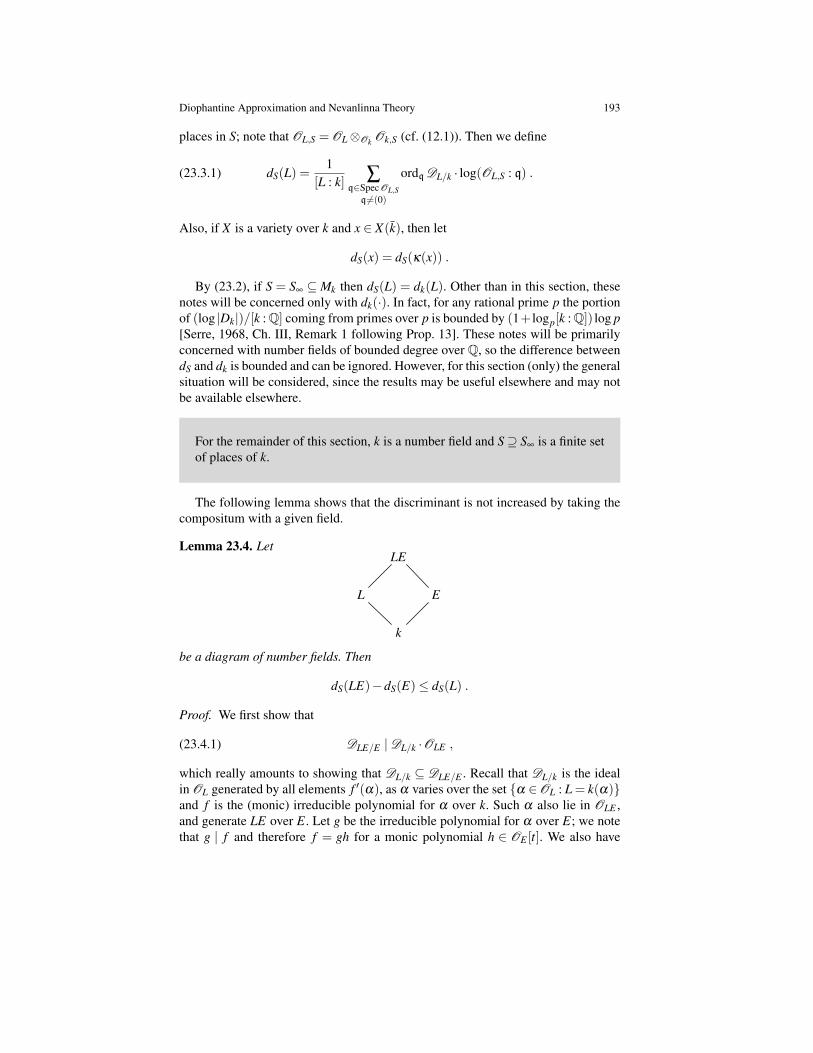
Diophantine Approximation and Nevanlinna Theory 193
places in S; note that OL,S = OL⊗Ok Ok,S (cf. (12.1)). Then we define
(23.3.1) dS(L) =1
[L : k] ∑q∈SpecOL,S
q6=(0)
ordq DL/k · log(OL,S : q) .
Also, if X is a variety over k and x ∈ X(k), then let
dS(x) = dS(κ(x)) .
By (23.2), if S = S∞ ⊆Mk then dS(L) = dk(L). Other than in this section, thesenotes will be concerned only with dk(·). In fact, for any rational prime p the portionof (log |Dk|)/[k : Q] coming from primes over p is bounded by (1+ logp[k : Q]) log p[Serre, 1968, Ch. III, Remark 1 following Prop. 13]. These notes will be primarilyconcerned with number fields of bounded degree over Q, so the difference betweendS and dk is bounded and can be ignored. However, for this section (only) the generalsituation will be considered, since the results may be useful elsewhere and may notbe available elsewhere.
For the remainder of this section, k is a number field and S⊇ S∞ is a finite setof places of k.
The following lemma shows that the discriminant is not increased by taking thecompositum with a given field.
Lemma 23.4. LetLE
L E
k
be a diagram of number fields. Then
dS(LE)−dS(E)≤ dS(L) .
Proof. We first show that
(23.4.1) DLE/E |DL/k ·OLE ,
which really amounts to showing that DL/k ⊆ DLE/E . Recall that DL/k is the idealin OL generated by all elements f ′(α), as α varies over the set α ∈OL : L = k(α)and f is the (monic) irreducible polynomial for α over k. Such α also lie in OLE ,and generate LE over E. Let g be the irreducible polynomial for α over E; we notethat g | f and therefore f = gh for a monic polynomial h ∈ OE [t]. We also have
194 Paul Vojta
f ′(α) = g′(α)h(α). Since h(α) ∈ OLE , it then follows that f ′(α) ∈ DLE/E , whichthen implies (23.4.1).
It then suffices to show that
ordq DL/k · log(OL : q) =1
[LE : L] ∑Q∈SpecOLE
Q|q
ordQ(DL/kOLE) · log(OLE : Q)
for all nonzero q ∈ SpecOL. But this follows immediately from the classical factthat [LE : L] = ∑eQ/q fQ/q. ut
The Chevalley-Weil theorem may be generalized to a situation where ramifi-cation is allowed. This involves a proximity function for the ramification divisor,which is defined as follows.
Definition 23.5. Let φ : X → Y be a generically finite, dominant morphism of non-singular complete varieties over a field k. Assume that the function field extensionK(X)/K(Y ) is separable. Then the natural map φ ∗ΩY/k → ΩX/k induces a natu-ral map φ ∗KY → KX of canonical sheaves, which in turn defines a natural mapOX →KX ⊗φ ∗K ∨
Y . This latter map defines a section of KX ⊗φ ∗K ∨Y , whose divi-
sor is the ramification divisor of X over Y . It is an effective divisor R, and we haveKX ∼= KY (R).
(The remainder of this section will be quite technical. Most readers will likelybe interested only in the statement of Theorem 23.15, and should now skip to thestatement of that theorem and to Theorem 23.17.)
The following definition will also be needed to generalize Chevalley-Weil.
Definition 23.6. Let M be a finitely generated module over a noetherian ring R, andlet
(23.6.1) Rm f−→ Rn −→M −→ 0
be a presentation of M. Then the 0th Fitting ideal of M is the ideal F0(M) in R gener-ated by the determinants of all n×n submatrices of the n×m matrix representing f .It is independent of the presentation [Eisenbud, 1995, 20.4]. This globalizes: if F isa coherent sheaf on a noetherian scheme X , then locally one can form presentations(23.6.1) and glue them to give a sheaf of ideals F0(F ).
Lemma 23.7. Let F be a coherent sheaf on a noetherian scheme X.
(a). Forming the Fitting ideal commutes with pull-back: Let φ : X ′→ X be a mor-phism of noetherian schemes. Then
(23.7.1) F0(φ ∗F ) = φ∗F0(F ) ·OX ′ .
(b). If F F ′ is a surjection, then
F0(F ′)⊇ F0(F ) .
Diophantine Approximation and Nevanlinna Theory 195
Proof. Let φ : X ′→ X be as in (a). Since tensoring is right exact, a presentation ofF pulls back to give a presentation of φ ∗F on X ′, and (23.7.1) follows directly.
If F F ′ is a surjection, then one can use the same middle terms in the localpresentations of F and of F ′, and the first term in the presentation of F can be adirect summand of the first term in the presentation of F ′. In this case, the resultinggenerators of F0(F ) are a subset of the generators of F0(F ′). This gives (b). ut
The ramification divisor can be described using a Fitting ideal.
Lemma 23.8. Let φ : X → Y be as in Definition 23.5. Then F0(ΩX/Y ) is a sheaf ofideals, locally principal and generated by functions f which locally generate theramification divisor as a Cartier divisor.
Proof. Indeed, the first exact sequence of differentials
φ∗ΩY/k −→ΩX/k −→ΩX/Y −→ 0
gives a locally free presentation of ΩX/Y , and the two initial terms have the samerank. ut
The proof of Theorem 23.15 will also need the notion of a model of a varietyover a number field (corresponding to Definition 15.2 in the function field case).
Definition 23.9. Let X be a variety over a number field k. A model for X over Ok isan integral scheme X , flat over Ok, together with an isomorphism X ∼= X ×Ok k.
If X is a complete variety, then a model X can be constructed using Nagata’s em-bedding theorem. Moreover, X can be chosen to be proper over SpecOk. On such amodel, rational points correspond naturally and bijectively to sections Ok→X bythe valuative criterion of properness, and algebraic points SpecL→ X correspondnaturally and bijectively to morphisms SpecOL→X over Ok.
As is the case over function fields, a key benefit of working with models is thefact that Weil functions, and therefore the proximity, counting, and height functions,can be defined exactly once one has chosen an extension of the given Cartier divisorD to the model. (Such an extension may not always exist, but the model can bechosen so that it does exist.) At archimedean places, these definitions rely on theadditional data specified in Arakelov theory. These definitions, however, will not bedescribed in these notes.
For the purposes of this section, however, we do need to define the proximityfunction relative to a sheaf of ideals.
Definition 23.10. Let X be a complete variety over a number field k, let X be aproper model for X over Ok, let I be a sheaf of ideals on X , and let S ⊇ S∞ be afinite set of places of k. Let x ∈ X(k), and assume that x does not lie in the closedsubscheme of X defined by I . Then the counting function NS(I ,x) is defined asfollows. Let L be some number field containing κ(x), let i : SpecOL →X be themorphism over SpecOk corresponding to x, and let I be the ideal in OL correspond-ing to the ideal sheaf i∗I ·OSpecOL on SpecOL. Then we define
196 Paul Vojta
NS(I ,x) =1
[L : k]log(OL,S : IOL,S)
=1
[L : k] ∑q∈SpecOL,S
q 6=(0)
ordq I · log(OL,S : q) .
It can be shown (although we will not do so here) that if X is a proper modelover SpecOk for a complete variety X over k, if I is an ideal sheaf on X , and ifthe restriction of I to X corresponds to a Cartier divisor D, then
(23.11) NS(I ,x) = NS(D,x)+O(1)
for all x ∈ X(k) not lying in SuppD.Counting (and proximity and height) functions relative to sheaves of ideals were
first introduced by Yamanoi [2004a], in the context of Nevanlinna theory.The different can be described via differentials as well. Indeed, DL/k is the anni-
hilator of the sheaf of relative differentials:
(23.12) DL/k = AnnΩOL/Ok.
In this case ΩOL/Okis a torsion sheaf locally generated by one element; hence
(23.3.1) can be rewritten as
dS(L) =1
[L : k] ∑q∈SpecOL,S
q6=(0)
lengthq ΩOL/Ok· log(OL,S : q)
=1
[L : k]log#H0(OL,S,ΩOL,S/Ok,S
) .
(23.13)
The following lemma does most of the work in generalizing the Chevalley-Weiltheorem. It has been stated as a separate lemma because it will also be used in theNevanlinna case.
Lemma 23.14. Let A→ B be a local homomorphism of discrete valuation rings,with B finite over A, let φ : X → Y be a generically finite morphism of schemes, andlet
(23.14.1)
SpecBj−−−−→ Xy yφ
SpecA −−−−→ Y
be a commutative diagram. Assume also that the image of j is not contained in thesupport of ΩX/Y , that j∗OX generates the fraction field of B over the fraction fieldof A, and that the fraction field of B is separable over the fraction field of A. Then
(23.14.2) DB/A ⊇ j∗F0(ΩX/Y ) ·B .
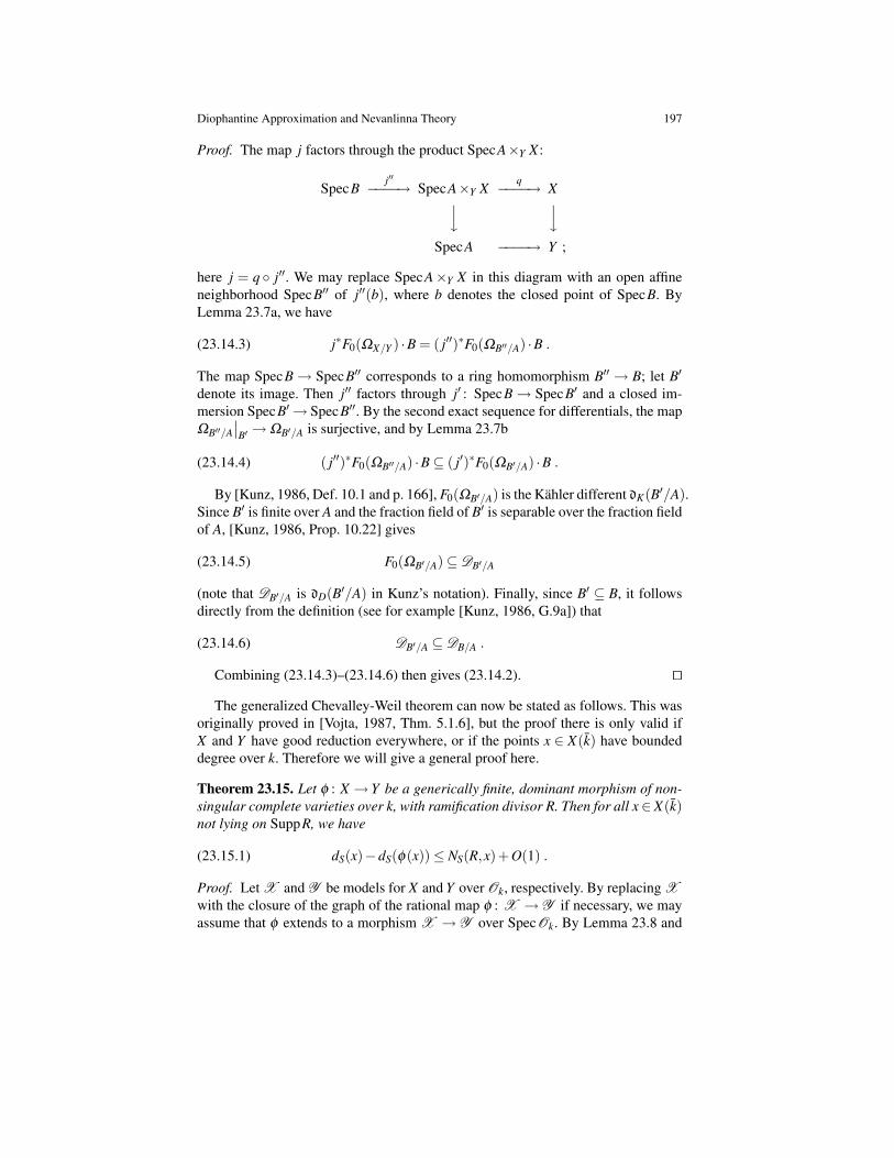
Diophantine Approximation and Nevanlinna Theory 197
Proof. The map j factors through the product SpecA×Y X :
SpecBj′′−−−−→ SpecA×Y X
q−−−−→ Xy ySpecA −−−−→ Y ;
here j = q j′′. We may replace SpecA×Y X in this diagram with an open affineneighborhood SpecB′′ of j′′(b), where b denotes the closed point of SpecB. ByLemma 23.7a, we have
(23.14.3) j∗F0(ΩX/Y ) ·B = ( j′′)∗F0(ΩB′′/A) ·B .
The map SpecB→ SpecB′′ corresponds to a ring homomorphism B′′ → B; let B′
denote its image. Then j′′ factors through j′ : SpecB→ SpecB′ and a closed im-mersion SpecB′→ SpecB′′. By the second exact sequence for differentials, the mapΩB′′/A
∣∣B′ →ΩB′/A is surjective, and by Lemma 23.7b
(23.14.4) ( j′′)∗F0(ΩB′′/A) ·B⊆ ( j′)∗F0(ΩB′/A) ·B .
By [Kunz, 1986, Def. 10.1 and p. 166], F0(ΩB′/A) is the Kahler different dK(B′/A).Since B′ is finite over A and the fraction field of B′ is separable over the fraction fieldof A, [Kunz, 1986, Prop. 10.22] gives
(23.14.5) F0(ΩB′/A)⊆DB′/A
(note that DB′/A is dD(B′/A) in Kunz’s notation). Finally, since B′ ⊆ B, it followsdirectly from the definition (see for example [Kunz, 1986, G.9a]) that
(23.14.6) DB′/A ⊆DB/A .
Combining (23.14.3)–(23.14.6) then gives (23.14.2). ut
The generalized Chevalley-Weil theorem can now be stated as follows. This wasoriginally proved in [Vojta, 1987, Thm. 5.1.6], but the proof there is only valid ifX and Y have good reduction everywhere, or if the points x ∈ X(k) have boundeddegree over k. Therefore we will give a general proof here.
Theorem 23.15. Let φ : X → Y be a generically finite, dominant morphism of non-singular complete varieties over k, with ramification divisor R. Then for all x∈ X(k)not lying on SuppR, we have
(23.15.1) dS(x)−dS(φ(x))≤ NS(R,x)+O(1) .
Proof. Let X and Y be models for X and Y over Ok, respectively. By replacing Xwith the closure of the graph of the rational map φ : X → Y if necessary, we mayassume that φ extends to a morphism X → Y over SpecOk. By Lemma 23.8 and
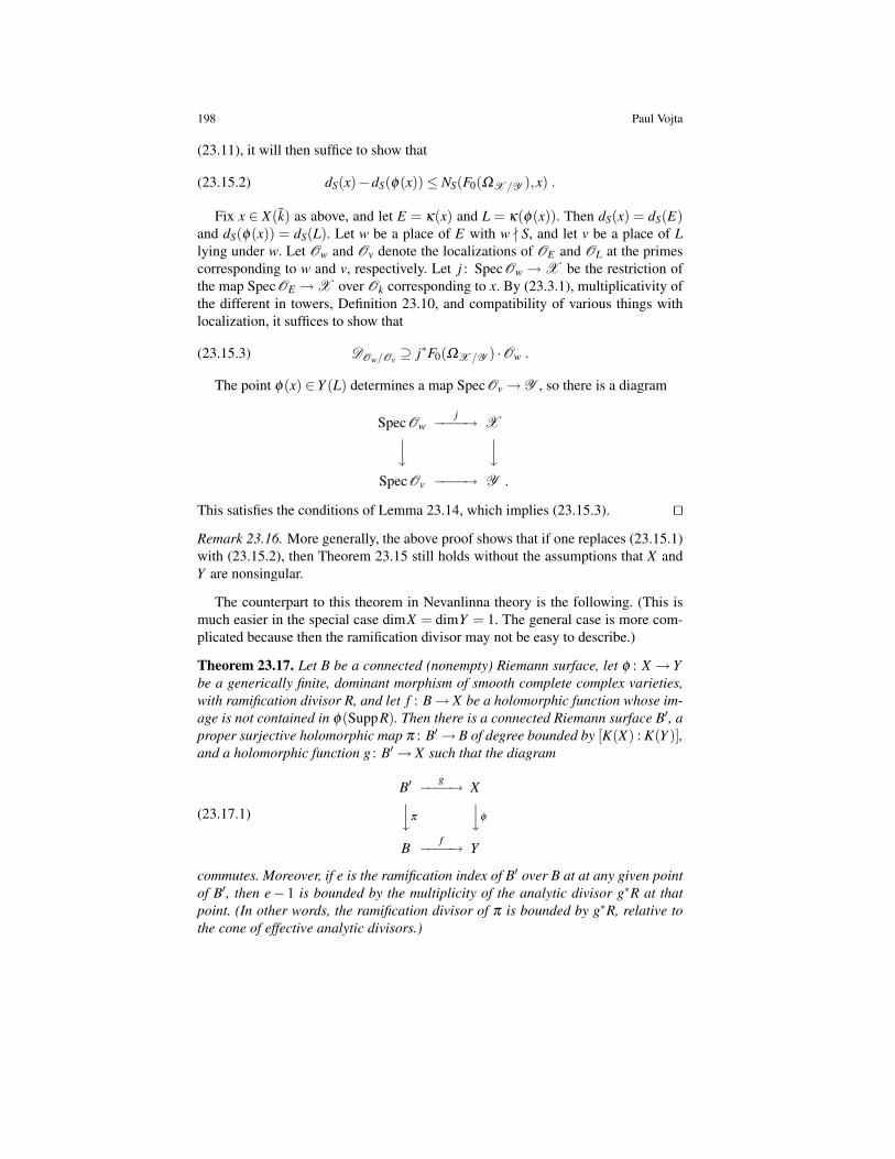
198 Paul Vojta
(23.11), it will then suffice to show that
(23.15.2) dS(x)−dS(φ(x))≤ NS(F0(ΩX /Y ),x) .
Fix x ∈ X(k) as above, and let E = κ(x) and L = κ(φ(x)). Then dS(x) = dS(E)and dS(φ(x)) = dS(L). Let w be a place of E with w - S, and let v be a place of Llying under w. Let Ow and Ov denote the localizations of OE and OL at the primescorresponding to w and v, respectively. Let j : SpecOw →X be the restriction ofthe map SpecOE →X over Ok corresponding to x. By (23.3.1), multiplicativity ofthe different in towers, Definition 23.10, and compatibility of various things withlocalization, it suffices to show that
(23.15.3) DOw/Ov ⊇ j∗F0(ΩX /Y ) ·Ow .
The point φ(x) ∈ Y (L) determines a map SpecOv→ Y , so there is a diagram
SpecOwj−−−−→ Xy y
SpecOv −−−−→ Y .
This satisfies the conditions of Lemma 23.14, which implies (23.15.3). ut
Remark 23.16. More generally, the above proof shows that if one replaces (23.15.1)with (23.15.2), then Theorem 23.15 still holds without the assumptions that X andY are nonsingular.
The counterpart to this theorem in Nevanlinna theory is the following. (This ismuch easier in the special case dimX = dimY = 1. The general case is more com-plicated because then the ramification divisor may not be easy to describe.)
Theorem 23.17. Let B be a connected (nonempty) Riemann surface, let φ : X → Ybe a generically finite, dominant morphism of smooth complete complex varieties,with ramification divisor R, and let f : B→ X be a holomorphic function whose im-age is not contained in φ(SuppR). Then there is a connected Riemann surface B′, aproper surjective holomorphic map π : B′→ B of degree bounded by [K(X) : K(Y )],and a holomorphic function g : B′→ X such that the diagram
(23.17.1)
B′g−−−−→ Xyπ
yφ
Bf−−−−→ Y
commutes. Moreover, if e is the ramification index of B′ over B at at any given pointof B′, then e− 1 is bounded by the multiplicity of the analytic divisor g∗R at thatpoint. (In other words, the ramification divisor of π is bounded by g∗R, relative tothe cone of effective analytic divisors.)
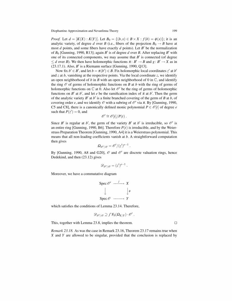
Diophantine Approximation and Nevanlinna Theory 199
Proof. Let d = [K(X) : K(Y )]. Let B0 = (b,x) ∈ B×X : f (b) = φ(x); it is ananalytic variety, of degree d over B (i.e., fibers of the projection B0 → B have atmost d points, and some fibers have exactly d points). Let B′ be the normalizationof B0 [Gunning, 1990, R13]; again B′ is of degree d over B. After replacing B′ withone of its connected components, we may assume that B′ is connected (of degree≤ d over B). We then have holomorphic functions π : B′→ B and g : B′→ X as in(23.17.1). Also, B′ is a Riemann surface [Gunning, 1990, Q13].
Now fix b′ ∈ B′, and let b = π(b′) ∈ B. Fix holomorphic local coordinates z′ at b′
and z at b, vanishing at the respective points. Via the local coordinate z, we identifyan open neighborhood of b in B with an open neighborhood of 0 in C, and identifythe ring O of germs of holomorphic functions on B at b with the ring of germs ofholomorphic functions on C at 0. Also let O ′ be the ring of germs of holomorphicfunctions on B′ at b′, and let e be the ramification index of π at b′. Then the germof the analytic variety B′ at b′ is a finite branched covering of the germ of B at b, ofcovering order e, and we identify O with a subring of O ′ via π . By [Gunning, 1990,C5 and C8], there is a canonically defined monic polynomial P ∈ O[t] of degree esuch that P(z′) = 0, and
O ′ ∼= O[t]/P(t) .
Since B′ is regular at b′, the germ of the variety B′ at b′ is irreducible, so O ′ isan entire ring [Gunning, 1990, B6]. Therefore P(t) is irreducible, and by the Weier-strass Preparation Theorem [Gunning, 1990, A4] it is a Weierstrass polynomial. Thismeans that all non-leading coefficients vanish at b. A straightforward computationthen gives
ΩO′/O = O ′/(z′)e−1 .
By [Gunning, 1990, A8 and G20], O and O ′ are discrete valuation rings, henceDedekind, and then (23.12) gives
DO′/O = (z′)e−1 .
Moreover, we have a commutative diagram
SpecO ′j−−−−→ Xy yφ
SpecO −−−−→ Y
which satisfies the conditions of Lemma 23.14. Therefore,
DO′/O ⊇ j∗F0(ΩX/Y ) ·O ′ .
This, together with Lemma 23.8, implies the theorem. ut
Remark 23.18. As was the case in Remark 23.16, Theorem 23.17 remains true whenX and Y are allowed to be singular, provided that the conclusion is replaced by
200 Paul Vojta
the assertion that the ramification divisor of π is bounded by the analytic divisorassociated to g∗F0(ΩX/Y ).
24 A Diophantine Conjecture for Algebraic Points
This section describes an extension of Conjecture 14.6 to allow algebraic pointsinstead of rational points. This comes at a cost of adding a discriminant term to theinequality.
This conjecture is subject to some doubt: see Remark 26.8.
Conjecture 24.1. Let k be a number field, let S⊇ S∞ be a finite set of places of k, letX be a smooth projective variety over k, let D be a normal crossings divisor on X ,let K be the canonical line sheaf on X , let A be an ample line sheaf on X , and letr be a positive integer. Then:
(a). Let Σ be a generic subset of X(k) \ SuppD such that [κ(x) : k] ≤ r for allx ∈ Σ . Then the inequality
(24.1.1) mS(D,x)+hK ,k(x)≤ dk(x)+O(log+ hA ,k(x))
holds for all x ∈ Σ .(b). For any ε > 0 there is a proper Zariski-closed subset Z of X , depending only
on X , D, A , and ε , such that for all C ∈ R the inequality
(24.1.2) mS(D,x)+hK ,k(x)≤ dk(x)+ ε hA ,k(x)+C
holds for almost all x ∈ (X \Z)(k) with [κ(x) : k]≤ r.
When r = 1, this just reduces to Conjecture 14.6, since then κ(x) = k for all x.Other than with r = 1, no case of this conjecture is known (for number fields). Overfunction fields, some parts are known.
One may also ask if the conjecture is true without the bound on r. This wouldrequire changing the quantization of C in part (b): for example, there are infinitelymany roots of unity, which all have height zero. It would also require changing thedk(x) terms to dS(x). Other than that, though, it seems to be a reasonable conjecture.
As with any mathematical statement, it is often useful to be aware of how itsstrength varies with the parameters. For this conjecture, replacing k with a largernumber field (and S with the corresponding set), adding places to S, increasing D,increasing r, or (in the case of part (b)) decreasing ε results in a stronger statement.
As was the case with Conjecture 14.6, this Conjecture 24.1 can also be posed forsmooth complete varieties X , provided that hA ,k is replaced by a big height.
Remark 14.7 does not extend trivially to Conjecture 24.1, though, since the dis-criminant terms may not add up.
Diophantine Approximation and Nevanlinna Theory 201
By [Vojta, 1987, Prop. 5.4.1],3 Conjecture 24.1b with D = 0 implies the fullConjecture 24.1b. This uses a covering construction.
Next, we show how Conjecture 24.1 relates to generically finite ramified covers.
Proposition 24.2. Let k and S be as in Conjecture 24.1, let π : X ′→ X be a surjec-tive generically finite morphism of complete nonsingular varieties over k, and letD be a normal crossings divisor on X. Let D′ = (π∗D)red (this means the reduceddivisor with the same support as π∗D), and assume that it too has normal crossings.Let K and K ′ denote the canonical line sheaves on X and X ′, respectively. Then,for all x ∈ X ′(k) not lying on SuppD′ or on the support of the ramification divisor,(24.2.1)
mS(D,π(x))+hK ,k(π(x))−dS(π(x))≤ mS(D′,x)+hK ′,k(x)−dS(x)+O(1) .
In particular, since the pull-back of any big line sheaf on X to X ′ remains big, eitherpart of Conjecture 24.1 for D′ on X ′ implies that same part for D on X.
Proof. Let R be the ramification divisor for X ′ over X ; since K ′ ∼= π∗K ⊗O(R),we then have
hK ,k(π(x))−hK ′,k(x) =−mS(R,x)−NS(R,x)+O(1) .
Also, Theorem 23.15 gives
dS(x)−dS(π(x))≤ NS(R,x)+O(1) .
Finally, by [Vojta, 1987, Lemma 5.2.2], π∗D− (π∗D)red ≤ R (relative to the cone ofeffective divisors). Therefore
mS(D,π(x))−mS(D′,x)≤ mS(R,x)+O(1) .
Adding this equation and the two inequalities then gives (24.2.1). ut
It was this proposition that motivated the original version of Conjecture 24.1[Vojta, 1987, p. 63].
Finally, we note that Conjecture 24.1 can also be posed with truncated countingfunctions.
Conjecture 24.3. Let k, S, X , D, K , A , and r be as in Conjecture 24.1. Then:
(a). Let Σ be a generic subset of X(k) \ SuppD such that [κ(x) : k] ≤ r for allx ∈ Σ . Then the inequality
(24.3.1) N(1)S (D,x)+dk(x)≥ hK (D),k(x)−O(log+ hA ,k(x))
holds for all x ∈ Σ .
3 The proposition is actually valid in more generality than its statement indicates. However, theproof has an error. The functions f1, . . . , fn must be chosen such that each point of SuppD has anopen neighborhood U such that D = ( fi) on U for some i.
202 Paul Vojta
(b). For any ε > 0 there is a proper Zariski-closed subset Z of X , depending onlyon X , D, A , and ε , such that for all C ∈ R the inequality
(24.3.2) N(1)S (D,x)+dk(x)≥ hK (D),k(x)− ε hA ,k(x)−C
holds for almost all x ∈ (X \Z)(k) with [κ(x) : k]≤ r.
Remark 24.4. Using a covering construction, it has been shown that Conjecture24.3b would follow from Conjecture 24.1b [Vojta, 1998]. As noted earlier in thissection, the latter would then follow from Conjecture 24.1b with D = 0, again usinga covering construction. In both of these cases, the coverings involved are generi-cally finite, so the implication holds for varieties of any given dimension. Thus, asis noted in the next section, Conjecture 24.3b has been fully proved for curves overfunction fields of characteristic 0.
Proposition 24.2 does not extend to the situation of truncated counting functions,though.
25 The 1+ ε Conjecture and the abc Conjecture
The special case of Conjecture 24.1 in which dimX = 1 and D = 0 is perhaps themost approachable unsolved special case, and has drawn some attention. It is calledthe “1+ ε conjecture.”
Conjecture 25.1. Let k be a number field, let X be a smooth projective curve over k,let K denote the canonical line sheaf on X , let r be a positive integer, let ε > 0, andlet C ∈ R. Then
hK ,k(x)≤ (1+ ε)dk(x)+C
for almost all x ∈ X(k) with [κ(x) : k]≤ r.
This conjecture was recently proved over function fields of characteristic 0 byMcQuillan [2008] and (independently) by Yamanoi [2004b]. See also McQuil-lan [2009] and Gasbarri [2008]. Thus, Conjectures 24.1 and 24.3 hold for curvesover function fields of characteristic 0, by Remark 24.4; see also [Yamanoi, 2004b,Thm. 5]
Conjecture 25.1 is known to imply the abc conjecture [Vojta, 1987, pp. 71–72].
Proposition 25.2. If Conjecture 25.1 holds, then so does the abc conjecture.
Proof. Let ε > 0, and let a,b,c be relatively prime integers with a+b+ c = 0. Forlarge integers n, there is an associated point
Pn =[
n√
a : n√b : n√
c]∈ Xn(Q) ,
where Xn is the nonsingular curve xn0 + xn
1 + xn2 = 0 in P2
Q. This point has height
Diophantine Approximation and Nevanlinna Theory 203
hK ,Q(Pn) =n−3
nlogmax|a|, |b|, |c|+O(1) ,
since the canonical line sheaf K on Xn is the restriction of O(n− 3). Here theimplicit constant depends only on n. We also have
dQ(Pn)≤n−1
n ∑p|abc
log p+O(1) ,
where the implicit constant depends only on n. Therefore, applying Conjecture 25.1to points Pn on Xn gives, for all n and all ε ′ > 0 a constant Cn,ε ′ ∈ R such that
n−3n
logmax|a|, |b|, |c| ≤(
n−1n
+ ε′)
∑p|abc
log p+Cn,ε ′ .
The proof concludes by taking n sufficiently large and ε ′ sufficiently small so that(n−1
n+ ε′)/ n−3
n< 1+ ε ,
and noting that the constants in the above discussion are independent of the triple(a,b,c). ut
26 Nevanlinna Theory of Finite Ramified Coverings
In Nevanlinna theory, changing the domain of the holomorphic function from Cto a finite ramified covering is the counterpart to working with algebraic points ofbounded degree.
References on finite ramified coverings include Lang and Cherry [1990, Ch. III]and Yamanoi [2004b].
Throughout this section, B is a connected Riemann surface, π : B→ C is aproper surjective holomorphic map, X is a smooth complete complex variety,and f : B→ X is a holomorphic function.
Note that π has a well-defined, finite degree, denoted degπ .We again refer to f as a holomorphic curve.
Definition 26.1. Define
B[r] = b ∈ B : |π(b)| ≤ r ,
B(r) = b ∈ B : |π(b)|< r , andB〈r〉= b ∈ B : |π(b)|= r .
204 Paul Vojta
On B〈r〉, let σ be the measure
σ =1
degππ∗(
dθ
2π
).
Definition 26.2. Let D be an effective divisor on X whose support does not containthe image of f , and let λD be a Weil function for D. Then the proximity functionof f with respect to D is
m f (D,r) =∫
B〈r〉λD f ·σ .
Definition 26.3. (a). The counting function for an analytic divisor ∆ = ∑b∈B
nb ·b
on B is
N∆ (r) =1
degπ
∑b∈B(r)\π−1(0)
nb logr
|π(b)|+ ∑
b∈π−1(0)
nb logr
.
(b). If D is a divisor on X whose support does not contain the image of f , thenthe counting function for D is the function
N f (D,r) = N f ∗D(r) .
(c). The ramification counting function for π is the counting function for theramification divisor of π . It is denoted NRam(π)(r).
If B = C and π is the identity mapping, then the proximity function of Definition26.2 and the counting function of Definition 26.3b extend those of Definitions 11.1and 11.2, respectively. They also satisfy additivity, functoriality, and boundednessproperties, as in Proposition 11.3.
If B′ is another connected Riemann surface and π ′ : B′ → B is another propersurjective holomorphic map, then
(26.4) m fπ ′(D,r) = m f (D,r) and N fπ ′(D,r) = N f (D,r) .
This holds in particular if B = C and π is the identity map. It is the counterpart tothe fact that the proximity and counting functions in number theory are independentof the choice of number field used in Definition 10.1.
In this situation (but without the assumption B = C), we also have
(26.5) NRam(ππ ′)(r) = NRam(π)(r)+NRam(π ′)(r) .
(Note that the first term on the right-hand side is a counting function on B, whilethe others are on B′.) This corresponds to multiplicativity of the different in towers.Note also that, although in general Ram(π) has infinite support, its support in anygiven set B(r) is finite, in parallel with the fact that any given extension of number
Diophantine Approximation and Nevanlinna Theory 205
fields has only finitely many ramified primes. However, given a sequence of alge-braic points of bounded degree, the corresponding sequence of number fields will ingeneral have no bound on the number of ramified primes, corresponding to the factthat Ram(π) may have infinite support.
The height is defined similarly to Definitions 11.4 and 11.7:
Definition 26.6. If D is an effective divisor on X whose support does not containthe image of f , then the height of f relative to D is defined up to O(1) by
TD, f (r) = m f (D,r)+N f (D,r) .
If L is a line sheaf on X , then the height TL , f (r) is defined to be TD, f (r) for anydivisor D on X for which O(D)∼= L and whose support does not contain the imageof f .
A First Main Theorem holds for the height as defined here, so the height relativeto a line sheaf is well defined [Lang and Cherry, 1990, III Thm. 2.1]. Theorem 11.8also holds for heights in this context, as do Propositions 11.10 and 11.11. Corollary11.9 is not meaningful in this context, since B need not be algebraic.
If π ′ : B′→ B is as in (26.4) and D and L are as in Definition 26.6, then
TD, fπ ′(r) = TD, f (r)+O(1) and TL , fπ ′(r) = TL , f (r)+O(1) .
Griffiths’ conjecture (Conjecture 14.2) can be posed in this context, withoutany changes other than the domain of the holomorphic curve f , and adding termsNRam(π)(r) to the right-hand sides of (14.2.1) and (14.2.2). It will not be repeatedhere.
The variant with truncated counting functions reads as follows.
Conjecture 26.7. Let X be a smooth complex projective variety, let D be a normalcrossings divisor on X , let K be the canonical line sheaf on X , and let A be anample line sheaf on X . Then:
(a). The inequality(26.7.1)
N(1)f (D,r)+NRam(π)(r)≥exc TK (D), f (r)−O(log+ TA , f (r))−o(logr)
holds for all holomorphic curves f : B→ X with Zariski-dense image.(b). For any ε > 0 there is a proper Zariski-closed subset Z of X , depending only
on X , D, A , and ε , such that the inequality
(26.7.2) N(1)f (D,r)+NRam(π)(r)≥exc TK (D), f (r)− ε TA , f (r)−C
holds for all nonconstant holomorphic curves f : B→ X whose image is notcontained in Z, and for all C ∈ R.
This is proved in many of the same situations where Conjecture 14.2 is proved(except possibly for the level of truncation of the counting functions). See for exam-ple [Lang and Cherry, 1990], and also Corollary 28.7 for the case when dimX = 1.
206 Paul Vojta
Remark 26.8. This conjecture, and therefore also Conjecture 24.1, is doubted bysome. For example, McQuillan [2000, Example V.1.5] notes that if X is a quotientof the unit ball in C2, if f : B→ X is a one-dimensional geodesic, and if π : B→ Cis a proper surjective holomorphic map, then
TKX , f (r) = NRam(π)(r)+o(TKX , f (r)) .
However, loc. cit. does not address how to show that a suitable map π exists, and insubsequent communications McQuillan has referred only to proper ramified cover-ings of the unit disk. Therefore, this is not strictly speaking a counterexample, butMcQuillan finds it persuasive.
27 The 1+ ε Conjecture in the Split Function Field Case
This section describes how the 1 + ε conjecture can be easily proved in what iscalled the “split function field case,” following early work of de Franchis [Lang,1983, p. 223].
Throughout this section, F is a field, B is a smooth projective curve over F ,and k = K(B) is the function field of B.
If L is a finite separable extension of k, corresponding to a smooth projectivecurve B′ over F and a finite morphism B′→ B over F , then the logarithmic discrim-inant term in the function field case is defined as
(27.1) dk(L) =degK ′
[L : k]−degK ,
where K ′ and K are the canonical line sheaves of B′ and B, respectively, anddegrees are taken relative to F . As before, we then define dk(x) = dk(κ(x)) forx ∈ X(k). The discriminant can also be written
(27.2) dk(L) =1
[L : k]dimF H0(B′,ΩB′/B)
(cf. (23.13)).This definition is valid for general function fields.The remainder of this section will restrict to the split function field case. This
refers to the situation in which X is of the form X ∼= X0×F k for a smooth projectivecurve X0 over F , the model X is a product X0×F B (so that the model splits into aproduct), and π : X → B is the projection morphism to the second factor.
Following early work of de Franchis [Lang, 1983, p. 223], it is fairly easy toprove the 1+ ε conjecture in the split function field case of characteristic 0.
Diophantine Approximation and Nevanlinna Theory 207
Theorem 27.3. Let F be a field of characteristic 0, let X0 be a smooth projectivecurve over F, let X = X0×F k, and let X = X0×F B. Let K be the canonical linesheaf on X0, and let A be an ample line sheaf on X0. View both of these line sheavesas line sheaves on X or on X by pulling back via the projection morphisms. Then
(27.3.1) hK ,k(x)≤ dk(x)+degΩB/F
for all x ∈ X(k).
Proof. The proof is particularly easy if F is algebraically closed.In that case, let q : X → X0 denote the projection morphism. If q i is a constant
morphism, then by (15.5) the left-hand side of (27.3.1) is zero. Since the right-handside is nonnegative by (27.2), the inequality is true in this case.
If q i is nonconstant, then it is finite and surjective, and we have
hK ,k(x) =(2g(X0)−2)deg(q i)
[K(B′) : k]≤ 2g(B′)−2
[K(B′) : k]= dk(x)+2g(B)−2 .
by (15.5), the Riemann-Hurwitz formula (twice), and by (27.1). (Here, as usual,g(B), g(B′), and g(X0) denote the genera of these curves.)
The general case proceeds by reducing to the above special case. First, we mayassume that F is algebraically closed in k (i.e., that k/F is a regular field extension).Indeed, replacing F with a finite extension divides both sides of (27.3.1) by thedegree of that extension, due to the fact that all quantities are expressed in terms ofdegrees of line sheaves, which depend in that way on F .
Let x be an algebraic point on X , let B′ be the smooth projective curve over Fcorresponding to κ(x), and let i : B′→X be the morphism over B corresponding tox. Again, K(B′) need not be a regular extension of F ; let F ′ be the algebraic closureof F in K(B′). We may replace X0 with X0×F F , B with B×F F , X with X ×F F ,and B′ with B′×F ′ F . This again does not affect the validity of (27.3.1), since bothsides are divided by [F ′ : F ]. Indeed, replacing B′ with B′×F F would have left bothsides of the inequality unchanged, but B′ would now be a disjoint union of [F ′ : F ]smooth projective curves. Choosing one of those curves amounts to taking B′×F ′ Finstead of B′×F F for some choice of embedding F ′ → F . Also, these changes donot affect the fact that X = X0×F B.
This reduces to the case in which F is algebraically closed. ut
A way to look at this proof is to think of the derivative of the map i : B′→X . Ittakes values in the absolute tangent bundle TX /F . Since X is a product, though, thetangent bundle is also a product p∗TX0/F ×q∗TB/F , where p and q are the projectionmorphisms. This allows us to project onto the second factor TX0/F , which gives away to bound TK ,k(x).
In the general (non-split) function field case, there is first of all no bundle TX0/Fto project to. Instead, we have only the relative tangent bundle TX /B. This is asubbundle of the absolute tangent bundle, not a quotient, and there is no canonicalprojection from TX /F to TX /B. McQuillan’s proof works mainly because, for pointsof large height, the tangent vectors giving the derivative of i : B′ →X are “more
208 Paul Vojta
vertical” than for points of smaller height. Therefore, two arbitrarily chosen ways ofprojecting the absolute tangent bundle to the relative tangent bundle will differ by asmaller amount, measured relative to the size of the tangent vector. This is sufficientto make the argument carry over.
28 Derivatives in Nevanlinna Theory
Generally speaking, proofs of theorems in Nevanlinna theory rely upon either oftwo methods for their basic proofs. Historically, the first was Nevanlinna’s “Lemmaon the Logarithmic Derivative” (Theorem 28.1). Slightly more recently, methodsusing differential geometry, especially focusing on curvature, have also been used.Although the latter has obvious geometric appeal, the method of the lemma on thelogarithmic derivative has also been phrased in geometric terms, and (at present) isthe preferred method for comparisons with number theory.
Throughout this section, B is a connected Riemann surface and π : B→ C isa proper surjective holomorphic map.
Nevanlinna’s original Lemma on the Logarithmic Derivative (LLD) is the fol-lowing.
Theorem 28.1. (Lemma on the Logarithmic Derivative) Let f be a meromorphicfunction on C. Then
(28.1.1)∫ 2π
0log+
∣∣∣∣ f ′(reiθ )f (reiθ )
∣∣∣∣ dθ
2π≤exc O(log+ Tf (r))+o(logr) .
More generally, if f is a meromorphic function on B, then
(28.1.2)∫
B〈r〉log+
∣∣∣∣d f /π∗dzf
∣∣∣∣σ ≤exc O(logTf (r)+ logr) .
Proof. For the first part, see [Nevanlinna, 1970, IX 3.3], or [Shiffman, 1983, Thm.3.11] for the error term given here. The second part follows from [Ashline, 1999,Thm. 2.2]. ut
A geometrical adaptation of this lemma has recently been discovered by R. Koba-yashi, M. McQuillan, P.-M. Wong, and others. This first requires a definition.
Definition 28.2. Let X be a smooth complex projective variety, and let D be a nor-mal crossings divisor on X . Then the sheaf Ω 1
X (logD) is the subsheaf of the sheaf ofmeromorphic sections of Ω 1
X generated by the holomorphic sections and the localsections of the form d f / f , where f is a local holomorphic function that vanishes
Diophantine Approximation and Nevanlinna Theory 209
only on D [Deligne, 1970, II 3.1]. This is locally free of rank dimX . The log tangentsheaf TX (− logD) is its dual. There are corresponding vector bundles, of the samenames.
Theorem 28.3. (Geometric Lemma on the Logarithmic Derivative) Let X be asmooth complex projective variety, let D be a normal crossings divisor on X, and letf : B→ X be a holomorphic curve whose image is not contained in SuppD. Let Abe an ample line sheaf on X. Finally, let | · | be a hermitian metric on the log tangentbundle TX (− logD), and let dD f : B→ TX (− logD) denote the canonical lifting off (as a meromorphic function). Then
(28.3.1)∫
B〈r〉log+∣∣dD f (reiθ )
∣∣σ ≤exc O(logTA , f (r)+ logr) .
Proof (Wong). The general idea of the proof is that one can work locally on finitelymany open sets to reduce the question to finitely many applications of the classicalLLD. This proof presents a geometric rendition of this idea.
We first note that the assertion is independent of the choice of metric, since bycompactness any two metrics are equivalent up to nonzero constant factors.
Next, note that the special case X = P1, D = [0]+[∞], is equivalent to the classicalLemma on the Logarithmic Derivative. Indeed, in this case TX (− logD)∼= X ×C isjust the trivial vector bundle of rank 1. Choose the metric on TX (− logD) to be theone corresponding to the obvious metric on X×C; then (28.3.1) reduces to (28.1.1).
The assertion of the theorem is preserved by taking products. Indeed, if it holdsfor holomorphic curves f1 : B→ X1 and f2 : B→ X2 relative to normal crossingsdivisors D1 and D2 on smooth complex projective varieties X1 and X2, respectively,then it is true for the product ( f1, f2) : B→ X1×X2 relative to the normal crossingsdivisor D := p∗1D1 + p∗2D2, where p j : X1×X2→ X j are the projection morphisms( j = 1,2). This follows by choosing the obvious metric on TX1×X2(− logD) andapplying (5.4.2); details are left to the reader.
Finally, let D′ be a normal crossings divisor on a smooth complex projectivevariety X ′, let Z be a closed subvariety of X that contains the image of f , and letφ : Z 99K X ′ be a rational map. Assume that there is a nonempty Zariski-open subsetU of Z and a constant C > 0 such that |φ∗(v)| ≥C|v| for all v ∈ TX (− logD) lyingover U , that the holomorphic curve f meets U , and that Theorem 28.3 holds forthe holomorphic curve φ f in X ′ relative to D′. We then claim that the theoremalso holds for f . Indeed, the left-hand side of (28.3.1) does not decrease by morethan logC if f is replaced by φ f , and the right-hand sides in the two cases arecomparable by Proposition 11.11 and properties of big line sheaves.
Therefore, we may assume that the divisor D has strict normal crossings. In-deed, there is a smooth complex projective variety X ′ and a birational morphismπ : X ′→ X , isomorphic over X \SuppD, such that D′ := (π∗D)red is a strict normalcrossings divisor. This is true because one can resolve the singularities of each com-ponent of D. Since π∗ induces a holomorphic map TX ′(− logD′)→ TX (− logD), theinverse rational map π−1 satisfies the conditions of the claim.
210 Paul Vojta
Thus, to prove the theorem, it suffices to let Z be the Zariski closure of the imageof f , and find nonzero elements f1, . . . , fn ∈ K(Z) for which the corresponding ra-tional map φ : Z 99K (P1)n satisfies the conditions of the claim (for suitable U ⊆ Zand C > 0) relative to the divisor D′ = ∑
nj=1 p∗j([0]+ [∞]), where p j : (P1)n→ P1 is
the projection morphism to the jth factor, 1≤ j ≤ n.To satisfy the conditions of the claim, it suffices to find a finite set G of nonzero
functions in K(X) such that at each closed point z ∈ Z there is a subset Gz ⊆ G suchthat for each g ∈ Gz the differential dg/g determines a regular section of Ω 1
X (logD)in a neighborhood of z in X , and such that as g varies over Gz the differentials dg/ggenerate Ω 1
X (logD) at z.To construct G , let z be a closed point of Z. For some open neighborhood V
of z in X there are regular functions g1, . . . ,gr on V whose vanishing determinesthe components of D passing through z in V . Letting m denote the maximal idealof z in X , the strict normal crossings condition implies that the g j are linearly in-dependent in the complex vector space m/m2 (the Zariski cotangent space). Aftershrinking V if necessary, we may choose regular functions gr+1, . . . ,gd on V , suchthat the functions g1, . . . ,gr,gr+1− 1, . . . ,gd − 1 all vanish at z, and such that theirimages in m/m2 form a basis. Then dg1/g1, . . . ,dgd/gd determine regular sectionsof Ω 1
X (logD) in a neighborhood of z in X , and generate the sheaf on that neighbor-hood. By a compactness argument, one then obtains a finite collection G satisfyingthe condition everywhere on Z. ut
Remark 28.4. There is no NRam(π)(r) term in either of these theorems; it appearssubsequently. The same is true of the exceptional set (it appears later still).
Remark 28.5. When B = C and π is the identity map, the error term in (28.3.1) canbe sharpened to O(log+ TA , f (r)) + o(logr). This will also be true in subsequentresults, but will not be explicitly mentioned.
The Geometric LLD leads to an inequality, due originally to McQuillan [1998,Thm. 0.2.5]. This inequality presently shows more promise for possible diophantineanalogies, since it omits some of the information on the derivative, and since it maybe related to parts of the proof of Schmidt’s Subspace Theorem.
Before stating the theorem, we note that for the purposes of these notes, if E is aquasi-coherent sheaf on a scheme X , then
P(E ) = Proj⊕d≥0
SdE
(as in EGA). In particular, if E is a vector sheaf, then points on P(E ) correspondbijectively to hyperplanes (not lines) in the fiber over the corresponding point onX . This scheme comes with a tautological line sheaf O(1), which gives rise to thename of McQuillan’s inequality.
If X and D are as in Theorem 28.3, then Ω 1X (logD) is defined as a locally free
sheaf on X as an analytic space. This is a coherent sheaf, hence by GAGA [Serre,1955–1956], it comes from a coherent sheaf on X as a scheme. This latter sheaf isdenoted ΩX/C(logD). In fact it is locally free—see the introduction to Section 29.
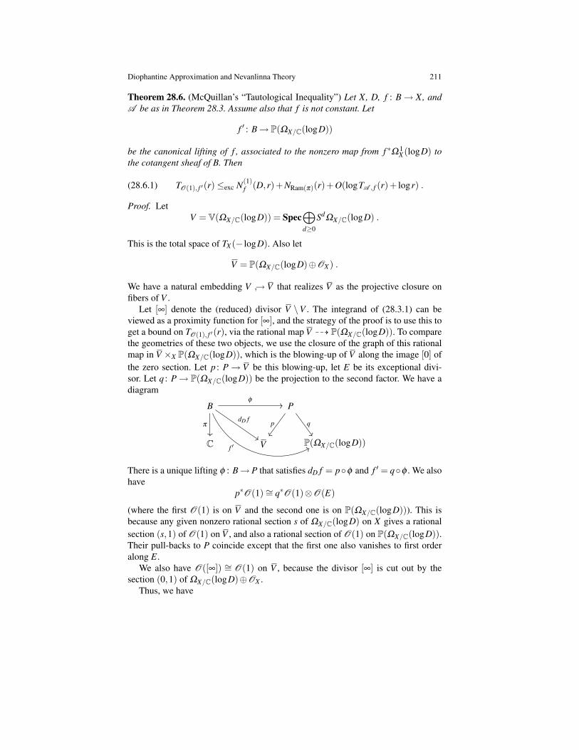
Diophantine Approximation and Nevanlinna Theory 211
Theorem 28.6. (McQuillan’s “Tautological Inequality”) Let X, D, f : B→ X, andA be as in Theorem 28.3. Assume also that f is not constant. Let
f ′ : B→ P(ΩX/C(logD))
be the canonical lifting of f , associated to the nonzero map from f ∗Ω 1X (logD) to
the cotangent sheaf of B. Then
(28.6.1) TO(1), f ′(r)≤exc N(1)f (D,r)+NRam(π)(r)+O(logTA , f (r)+ logr) .
Proof. LetV = V(ΩX/C(logD)) = Spec
⊕d≥0
SdΩX/C(logD) .
This is the total space of TX (− logD). Also let
V = P(ΩX/C(logD)⊕OX ) .
We have a natural embedding V → V that realizes V as the projective closure onfibers of V .
Let [∞] denote the (reduced) divisor V \V . The integrand of (28.3.1) can beviewed as a proximity function for [∞], and the strategy of the proof is to use this toget a bound on TO(1), f ′(r), via the rational map V 99K P(ΩX/C(logD)). To comparethe geometries of these two objects, we use the closure of the graph of this rationalmap in V ×X P(ΩX/C(logD)), which is the blowing-up of V along the image [0] ofthe zero section. Let p : P→ V be this blowing-up, let E be its exceptional divi-sor. Let q : P→ P(ΩX/C(logD)) be the projection to the second factor. We have adiagram
P
V P(ΩX/C(logD))
p q
B
C
π
φ
dD f
f ′
There is a unique lifting φ : B→ P that satisfies dD f = pφ and f ′ = qφ . We alsohave
p∗O(1)∼= q∗O(1)⊗O(E)
(where the first O(1) is on V and the second one is on P(ΩX/C(logD))). This isbecause any given nonzero rational section s of ΩX/C(logD) on X gives a rationalsection (s,1) of O(1) on V , and also a rational section of O(1) on P(ΩX/C(logD)).Their pull-backs to P coincide except that the first one also vanishes to first orderalong E.
We also have O([∞]) ∼= O(1) on V , because the divisor [∞] is cut out by thesection (0,1) of ΩX/C(logD)⊕OX .
Thus, we have
212 Paul Vojta
TO(1), f ′(r) = Tq∗O(1),φ (r)+O(1)
= TO(1),dD f (r)−TO(E),φ (r)+O(1)
= NdD f ([∞],r)−TO(E),φ (r)+mdD f ([∞],r)+O(1)
≤exc N(1)f (D,r)+NRam(π)(r)+O(logTA , f (r)+ logr) .
To explain the last step above, mdD f ([∞],r) is bounded by Theorem 28.3. Since Eis effective and does not contain the image of φ (since f is not constant), TO(E),φ (r)is bounded from below. (It can also be used to subtract a term NRam( f )(r) from theright-hand side of (28.6.1).)
Now consider NdD f ([∞],r). Fix a point b ∈ B, let w be a local coordinate on Bat b, let z be the coordinate on C, and let z1, . . . ,zn be local coordinates on X atf (b) such that D is locally given by z1 · · ·zr = 0 nearby. Then, near f (b), V hashomogeneous coordinate functions dz1/z1, . . . ,dzr/zr,dzr+1, . . . ,dzn,1. Relative tothese coordinates, the value of dD f in a punctured neighborhood of b is given by[
d(z1 f )/dzz1 f
: · · · : d(zr f )/dzzr f
:d(zr+1 f )
dz: · · · : d(zn f )
dz: 1]
=[
d(z1 f )/dwz1 f
: · · · : d(zr f )/dwzr f
:d(zr+1 f )
dw: · · · : d(zn f )
dw:
dzdw
].
Then dD f will meet [∞] to the extent that there are poles among the first n coor-dinates or a zero in the last coordinate. Poles among the first n coordinates canonly occur in the first r coordinates (using the second representation above), and inthat case they will at most be simple poles and will only occur if f (b) ∈ SuppD.Thus the contribution to NdD f ([∞],r) from poles in these coordinates is bounded byN(1)
f (D,r). The contribution coming from zeroes in the last coordinate is boundedby NRam(π)(r). ut
As a sample application of this theorem, it implies the Second Main Theoremwith truncated counting functions for maps to Riemann surfaces, including thecase in which the domain is a finite ramified cover of C. This is the (proved) casedimX = 1 of Conjecture 26.7.
Corollary 28.7. Let X be a smooth complex projective curve, let D be an effectivereduced divisor on X, and let f : B→ X be a non-constant holomorphic curve. Then
(28.7.1) N(1)f (D,r)+NRam(π)(r)≥exc TK (D), f (r)−O(logTA , f (r)+ logr) .
Proof. Since X is a curve, the vector sheaf ΩX/C(logD) is isomorphic to the linesheaf K (D). Therefore the canonical projection p : P(ΩX/C(logD))→ X is an iso-morphism, O(1)∼= p∗K (D), and f ′ = p−1 f . Thus
TO(1), f ′(r) = TK (D), f (r)+O(1) ,
so (28.7.1) is equivalent to (28.6.1). ut
Diophantine Approximation and Nevanlinna Theory 213
Remark 28.8. In fact, when dimX = 1, McQuillan’s inequality is directly equivalentto Conjecture 26.7, as can be seen from the above proof. This is not true in higherdimension, though (McQuillan’s inequality is proved, but Conjecture 26.7 is not).
Cartan’s theorem (Theorem 7.7) can also be proved using McQuillan’s inequal-ity, but this requires more work than can be included here. See [Vojta, 2008]. Themodified version (Theorem 7.13) requires a modified form of McQuillan’s inequal-ity (involving the same type of change).
It is hoped that other key results in Nevanlinna theory can also be proved usingTheorem 28.6.
We end the section with another corollary, which often has applications in Nevan-linna theory. It generalizes the Schwarz lemma, which has played an important rolein Nevanlinna theory for a long time; see [Siu and Yeung, 1997, Thm. 3], where itis proved for jet differentials. The introduction of op. cit. also describes some of thehistory of this result. See also [Lu, 1991, § 4], [Vojta, 2000, Cor. 5.2], and [Vojta,2001].
Corollary 28.9. Let X be a smooth complex projective variety, let D be a normalcrossings divisor on X, let f : B→ X be a holomorphic map, let A be an ample linesheaf on X, let L be a line sheaf on X, let d be a positive integer, and let ω be aglobal section of SdΩX/C(logD). If f ∗ω 6= 0 (i.e., it does not vanish everywhere onB), then
1d
TL , f (r)≤exc N(1)f (D,r)+NRam(π)(r)+O(logTA , f (r)+ logr) .
Proof. Let f ′ : B→ P(ΩX/C(logD)) be as in Theorem 28.6, and let
p : P(ΩX/C(logD))→ X
be the canonical projection. Then ω corresponds to a global section
ω′ ∈ Γ
(P(ΩX/C(logD)),O(d)⊗ p∗L ∨) ,
and ( f ′)∗ω ′ = f ∗ω . Thus the image of f ′ is not contained in the base locus ofO(d)⊗L ∨, so
TO(d), f ′(r)≥ TL , f (r)+O(1)
by Theorem 11.8c. The result then follows immediately from (28.6.1). ut
One can think of this result as a generalization of the fact that if f : C → Xis a nonconstant map from a nonsingular projective curve of genus g to a smoothcomplete variety X , then deg f ∗KX ≤ 2g−2, where KX is the canonical line sheafof X . Thus, it is useful in carrying over results from the split function field case toNevanlinna theory (see Section 17). It is used in this manner in the proof of [Vojta,2000, Thm. 5.3].
214 Paul Vojta
29 Derivatives in Number Theory
Whether one uses the Lemma on the Logarithmic Derivative or curvature, Nevan-linna theory depends in an essential way on the ability to take the derivative of aholomorphic function. In the number field case, on the other hand, there is currentlyno known counterpart to the derivative. Even in the function field case, the deriva-tive lives in the absolute tangent bundle, but any counterpart to the derivative as inNevanlinna theory should live in the relative tangent bundle. McQuillan gets aroundthis in his proof of the 1+ ε conjecture, by noting that for points of large height thederivative has an approximate projection to the relative tangent bundle that is pre-cise enough to be useful (see the end of Section 27). Although this method shows agreat deal of promise, it will not be explored further here.
Instead, this section will describe a conjecture in number theory based on Mc-Quillan’s tautological inequality. Because of its origin, the name “tautological con-jecture” is too good to pass up.
If X is a smooth complete variety over a field k, and if D is a normal crossingsdivisor on X , then an algebraic definition of ΩX/k(logD) is given in [Kato, 1989,1.7]. Kato [1989, 1.8] also shows this to be locally free in the etale topology of rankdimX . This then descends to a quasi-coherent sheaf on X in the Zariski topology by[Grothendieck et al., 1971, VIII Thm. 1.1]. It is a vector sheaf (with non-obviousgenerators) by [Grothendieck and Dieudonne, 1960–1967, IV 2.5.2].
Conjecture 29.1. (Tautological Conjecture) Let k be a number field, let S ⊇ S∞ bea finite set of places of k, let X be a nonsingular complete variety over k withdimX > 0, let D be a normal crossings divisor on X , let r be a positive integer,let A be an ample line sheaf on X , and let ε > 0. Then, for all x ∈ X(k) \SuppDwith [κ(x) : k]≤ r, there is a closed point x′ ∈ P(ΩX/k(logD)) lying over x such that
(29.1.1) hO(1),k(x′)≤ N(1)
S (D,x)+dk(x)+ ε hA ,k(x)+O(1) .
Moreover, given a finite collection of rational maps gi : X 99KWi to varieties Wi,there are finite sets Σi of closed points on Wi for each i with the following prop-erty. For each x as above, x′ may be chosen so that, for each i, if x lies in the do-main of gi and if gi(x) /∈ Σi, then x′ lies in the domain of the induced rational mapP(ΩX/k(logD)) 99K P(ΩWi/k). Moreover, the constant implicit in the O(1) term de-pends only on k, S, X , D, r, A , ε , the rational maps gi, and the choices of heightand counting functions.
This extra condition (involving the rational maps gi) should perhaps be explaineda bit. This condition seems to be necessary in order to ensure that the points x′
behave more like derivatives. For example, consider the special case in which r = 1,D = 0, and X is a product X1×X2. Then the points x must be rational points, and(29.1.1) for X is the sum of the same inequality for X1 and X2. But then, withoutthe last condition in the conjecture, the conjecture would hold if it held for eitherfactor, since one could take x′ tangent to the copy of X1 or X2 sitting inside of X .This seems a bit unnatural. In addition, the last condition is useful for applications.
Diophantine Approximation and Nevanlinna Theory 215
McQuillan’s work is not the only support for this conjecture. For some time, ithas been known that parts of Schmidt’s proof of his Subspace Theorem correspondto a proof of Cartan’s theorem due to H. and J. Weyl [Weyl and Weyl, 1938], fur-ther developed by L. Ahlfors [1941]. Both of these proofs can be divided up intoan “old” part (corresponding to an extension to higher dimensions of the proofs ofRoth and Nevanlinna of the earlier case on P1), and a “new” part. In Ahlfors’ case,the “new” part consists of working with the associated curves (Frenet formalism);in Schmidt’s case, it consists of working with Minkowski’s theory of successiveminima. In either case, the proof involves geometric constructions on
∧p Cn+1 or∧p kn+1, respectively. This strongly suggested that the theory of successive min-ima may be related to the use of derivatives in number theory [Vojta, 1987, Ch. 6].This has been recently refined [Vojta, 2008] to more explicitly involve a variant ofConjecture 29.1, and also to use the geometry of flag varieties.
The tie-in between successive minima and the tautological conjecture proceedsas follows. Let X be a nonsingular complete variety over a number field k, let D be anormal crossings divisor on X , let Y = SpecOk, and let X → Y be a proper modelfor X . Then we have a relative tangent sheaf TX /Y (− logD) on X . This is not nec-essarily a vector sheaf, since X need not be smooth over Y and D need not extendas a normal crossings divisor. However, we shall ignore that distinction for the sakeof discussion. Via the mechanisms of Arakelov theory, one can assign a Hermitianmetric to the sheaf at all archimedean places. If i : SpecY →X is the section ofX → Y corresponding to a given rational point, then i∗TX /Y (− logD) is a vectorsheaf on Y = SpecOk, which can then be viewed as a lattice in Rn (if k = Q), or as alattice in (k⊗Q R)n (generally). Bounds on the metrics at archimedean places corre-spond to giving a convex symmetric body in (k⊗Q R)n, and therefore Minkowski’stheory of successive minima can be translated into Arakelov theory as a search forlinearly independent nonzero sections of i∗TX /Y (− logD), obeying certain upperbounds on its metric at each infinite place. See, for example, [Gillet and Soule,1991]. Or, in the function field case, it is known that Minkowski’s theory corre-sponds to a search for nonzero global sections with bounded poles at certain places(an application of Riemann-Roch).
Giving a nonzero section as the first successive minimum is basically equivalentto giving a line subsheaf of largest degree (unless the first two successive minimaare close). This corresponds to giving a quotient subbundle L of i∗ΩX /Y (logD)of smallest degree. This, in turn, corresponds to giving a point x′ ∈ P(ΩX/Y (logD))lying over the rational point in question [Hartshorne, 1977, II 7.12]. The sheaf Lis none other than the pull-back of the tautological bundle O(1) to Y via the sectioni′ : Y → P(ΩX /Y (logd)) corrsponding to the point x′. Therefore, the degree of Lis the height hO(1),k(x′) (see (15.5)). This again leads to Conjecture 29.1.
We emphasize that specific bounds on the O(1) term in (29.1.1) are not given, soConjecture 29.1 is meaningful only for an infinite set of points—or, better yet, for ageneric or semi-generic set of points (Definitions 14.5 and 14.11).
Remark 29.2. The assertions of Remark 28.8 also apply in the arithmetic situation.When dimX = 1, the extra conditions involving the rational functions gi in the Tau-tological Conjecture are automatically satisfied. Therefore, in this case the Tautolog-

216 Paul Vojta
ical Conjecture is equivalent to Conjecture 24.3b (for the same reasons as in Remark28.8). Thus, by Remark 24.4, the Tautological Conjecture is proved for curves overfunction fields of characteristic 0. As in Remark 28.8, though, Conjectures 29.1 and24.3b are not as closely related when dimX > 1.
We also note that points of low height as in Conjecture 29.1 behave like deriva-tives in the following sense.
Proposition 29.3. (Arithmetic Chain Rule) Let f : X1 → X2 be a morphism ofcomplete varieties over a number field k. Then, for all x ∈ X1(k) where f isetale, and for all closed points x′ ∈ P(ΩX1/k) lying over x, the rational mapf∗ : P(ΩX1/k) 99K P(ΩX2/k) takes x′ to a point x′2 (lying over f (x)) for which
hO(1),k(x′2)≤ hO(1),k(x
′)+O(1) .
Moreover, assume that X1 and X2 are projective, with ample line sheaves A1 andA2, respectively, and that ε1 > 0 is a positive number for which (29.1.1) holds forall x in some set Σ ⊆ X1(k) (with respect to A1 and ε1). Then there is an ε2 > 0 suchthat (29.1.1) holds for f (x) ∈ X2(k) for all x ∈ Σ , with respect to A2 and ε2.
Proof. Let X1 and X2 be models for X1 and X2 over Y := SpecOk, respectively,chosen such that f extends as a morphism f : X1 → X2, let Y ′ = SpecOκ(x′),and let i : Y ′ →X1 be the multisection corresponding to x (which factors throughSpecOκ(x)). Then x′ corresponds to a surjection i∗ΩX1/Y L for a line sheaf Lon Y ′, and hO(1),k(x′) is the Arakelov degree of L divided by [κ(x′) : k]. We alsohave a morphism f ∗ΩX2/Y → ΩX1/Y , isomorphic at x. This gives a nonzero map( f i)∗ΩX2/Y →L , so hO(1),k(x′2) ≤ hO(1),k(x′) (with heights defined using thesemodels).
The second assertion is immediate from the first assertion, by Proposition 9.15.ut
A similar result holds for closed immersions (but without the assumption onetaleness).
The name “Arithmetic Chain Rule” comes from the fact that this result showsthat the “derivatives” x′ and x′2 are related in the expected way.
30 Another Conjecture Implies abc
Conjecture 22.5, involving truncated counting functions, is of course a vast general-ization of the abc conjecture, and Conjecture 24.1, which involved algebraic points,also rather easily implies abc. Actually, though, the (seemingly) weaker Conjec-ture 14.6 has also been shown to imply the abc conjecture [Vojta, 2000]. This im-plication, however, (necessarily) needs to use varieties of dimension > 1, whereasknowing either of the former two conjectures even for curves would suffice.
This section sketches the proof of the implication mentioned above.
Diophantine Approximation and Nevanlinna Theory 217
Theorem 30.1. For any ε > 0 there is a nonsingular projective variety Xε over Q, anormal crossings divisor Dε on Xε , and a real number ε ′> 0, such that if Conjecture14.6b holds for Xε , Dε , and ε ′, then the abc conjecture (Conjecture 22.6) holds forε .
Proof (sketch). Fix an integer n > 3/ε +3. Let Xn be the closed subvariety in(P2)n
in coordinates([x1 : y1 : z1], . . . , [xn : yn : zn])
given by the equationn
∏i=1
xii +
n
∏i=1
yii +
n
∏i=1
zii = 0 .
There is a rational map Xn 99K P2 given by
(30.1.1) ([x1 : y1 : z1], . . . , [xn : yn : zn]) 7→[∏xi
i : ∏yii : ∏zi
i]
.
Let Γn be the closure of the graph of this rational map in Xn×P2, and let φ : Γn→ P2
be the projection to the second factor. The image of φ is a line, which we identifywith P1.
Given relatively prime integers a,b,c with a+b+c = 0, define a point in Xn(Q)as follows. Let
xn = ∏p
p[(ordp a)/n] and xi = ∏ordp a≡i (mod n)
p (i < n) .
(The brackets in the definition of xn denote the greatest integer function.) With thesedefinitions, we have a = ∏xi
i, with xn as large as possible subject to all xi beingintegers. Similarly define y1, . . . ,yn using b and z1, . . . ,zn using c. This point lifts toa unique point in Γn(Q), which we denote Pa,b,c.
Let D be the effective Cartier divisor on Γn obtained by pulling back the divisorx1 · · ·xny1 · · ·ynz1 · · ·zn = 0 from Xn, and let E be the divisor on the image P1 of φ ,obtained by restricting the coordinate hyperplanes on P2. The latter divisor is thesum of the points [1 : −1 : 0], [0 : 1 :−1], and [−1 : 0 : 1]. Let S = ∞ ⊆MQ. It ispossible to show that if p is a rational prime and v is the corresponding place of Q,then
λE,v([a : b : c]) = ordp(abc) log p
andλD,v(Pa,b,c) = ordp(x1 · · ·xny1 · · ·ynz1 · · ·zn) log p ,
using Weil functions suitably defined using (7.9.1). It then follows that
NS(D,Pa,b,c)≤ ∑p|abc
log p+1n
NS(E,φ(Pa,b,c)) .
One would like to apply Conjecture 14.6 to the divisor D on Γn, but this is notpossible since Γn is singular. However, there is a nonsingular projective variety Γ ′n ,
218 Paul Vojta
a normal crossings divisor D′ on Γ ′n , and a proper birational morphism ψ : Γ ′n → Γn,such that SuppD′ = ψ−1(SuppD), ψ is an isomorphism over a suitably large set,and KΓ ′n (D′) ≥ ψ∗φ ∗O(1) relative to the cone of effective divisors. For details see[Vojta, 2000, Lemma 3.9].
Let P′a,b,c be the point on Γ ′n lying over Pa,b,c. Then one can show that
hQ([a : b : c]) = hψ∗φ∗O(1),Q(P′a,b,c)+O(1)
≤ hKΓ ′n
(D′),Q(P′a,b,c)+O(1)
≤ NS(D′,P′a,b,c)+ ε′hA ,Q(P′a,b,c)+O(1)
≤ NS(D,Pa,b,c)+ ε′hA ,Q(P′a,b,c)+O(1)
≤ ∑p|abc
log p+3n
hQ([a : b : c])+ ε′′hQ([a : b : c])+O(1)
≤ ∑p|abc
log p+ε
1+ εhQ([a : b : c])+O(1) ,
and therefore hQ([a : b : c]) ≤ (1 + ε)∑p|abc log p + O(1). Here we have used thefact that NS(D′,P′a,b,c)≤ NS(D,Pa,b,c), which follows from the fact that ψ∗D−D′ iseffective.
This chain of inequalities holds outside of some proper Zariski-closed subset ofΓ ′n , but it is possible to show that this set can be chosen so that it only involvesfinitely many triples (a,b,c). ut
The variety Xn admits a faithful action of G2n−2m , by letting the first n− 1 coor-
dinates act by xi 7→ txi and x1 7→ t−ix1 for i = 2, . . . ,n, and letting the other n− 1coordinates act similarly on the yi. This action respects fibers of the rational map(30.1.1), so the action extends to Γn, and the construction of Γ ′n can be done so thatthe group action extends there, too. Since dimXn = 2n− 1, the group acts transi-tively on open dense subsets of suitably generic fibers of φ . It is this group actionthat allows one to control the proper Zariski-closed subset of Γ ′n arising out of Con-jecture 14.6b. The group action also provides some additional structure, and in factConjecture 14.2 can be proved in this context [Vojta, 2000, Thm. 5.3].
31 An abc implication in the other direction
The preceding sections give a number of ways in which some conjectures implythe abc conjecture. It is also true, however, that the abc conjecture implies partsof the preceding conjectures. While this is mostly a curiousity, since the impliedspecial cases are known to be true whereas the abc conjecture is still a conjecture,this provides some insight into the geometry of the situation.
The implications of this section were first observed by Elkies [1991], whoshowed that “Mordell is as easy as abc,” i.e., the abc conjecture implies the Mordell
Diophantine Approximation and Nevanlinna Theory 219
conjecture. This was extended by Bombieri [1994], who showed that abc impliesRoth’s theorem, and then by van Frankenhuijsen [2002], who showed that the abcconjecture implies Conjecture 14.6b for curves. In each of these cases, the abc con-jecture for a number field k would be needed to imply any given instance of Con-jecture 14.6b. Here “the abc conjecture for k” means Conjecture 22.5b over k withX = P1
k and D = [0] + [1] + [∞]. It is further true that a “strong abc conjecture,”namely Conjecture 24.3b with X = P1
k and D = [0] + [1] + [∞], would imply Con-jecture 24.1b for curves; in other words van Frankenhuijsen’s implication holds alsofor algebraic points of bounded degree.
This circle of ideas stems from two observations. The first of these is due to Belyı[1979]. He showed that a smooth complex projective curve X comes from a curveover Q (i.e., there is a curve X0 over Q such that X ∼= X0×Q C) if and only if there isa finite morphism from X to P1
C ramified only over 0,1,∞. For our purposes, thiscan be adapted as follows.
Theorem 31.1. (Belyı) Let X be a smooth projective curve over a number fieldk, and let S be a finite set of closed points on X. Then there is a finite morphismf : X → P1
k which is ramified only over 0,1,∞, and such that S⊆ f−1(0,1,∞).
Proof. See Belyı [1979] or Serre [1989]. ut
The other ingredient is a complement (and actually, a converse) to Proposition24.2, using truncated counting functions.
Proposition 31.2. Let k be a number field or function field, let S ⊇ S∞ be a finiteset of places of k, let π : X ′ → X be a surjective generically finite morphism ofcomplete nonsingular varieties over k, and let D be a normal crossings divisor onX. Let D′ = (π∗D)red, and assume that it too has normal crossings. Assume also thatthe ramification divisor R of π satisfies
(31.2.1) R = π∗D−D′
(and therefore that π is unramified outside of SuppD′).4 Let K and K ′ denote thecanonical line sheaves on X and X ′, respectively. Then, for all x ∈ X ′(k) not lyingon SuppD′,
N(1)S (D′,x)+dS(x)−hK ′(D′),k(x)
≥ N(1)S (D,π(x))+dS(π(x))−hK (D),k(π(x))+O(1) ,
(31.2.2)
with equality if [κ(x) : k] is bounded. In particular, either part of Conjecture 24.3for D′ on X ′ is equivalent to that same part for D on X.
Proof. First, by (31.2.1), we have K ′(D′)∼= π∗(K (D)). Thus
4 This condition is equivalent to (X ′,D′) being log etale over (X ,D) by [Kato, 1989, (3.12)], usingthe fact that (X ′,D′) is log smooth over Speck by (3.7)(1) of op. cit.
220 Paul Vojta
hK ′(D′),k(x) = hK (D),k(π(x))+O(1) ,
so it suffices to show that
(31.2.3) N(1)S (D′,x)+dS(x)≥ N(1)
S (D,π(x))+dS(π(x))+O(1) ,
with equality if [κ(x) : k] is bounded.Now let YS = SpecOk,S (or, if S = /0, which can only happen in the function
field case, let YS be the smooth projective curve over the field of constants of k forwhich K(YS) = k). Let X be a proper model for X over YS for which D extendsto an effective Cartier divisor, which will still be denoted D. (This can be obtainedby taking a proper model, extending D to it as a Weil divisor, and blowing up thesheaf of ideals of the corresponding reduced closed subscheme.) Let X ′ be a propermodel for X ′ over YS. We may assume that π extends to a morphism π : X ′→X ,and that D′ extends to an effective Cartier divisor on X ′. We assume further thatSuppD′ = π−1(SuppD) (on X ′). Indeed, one can obtain X ′ and D′ by blowing upthe reduced sheaf of ideals corresponding to π−1(SuppD).
For x ∈ X ′(k), let L = κ(π(x)), let L′ = κ(x), and let Y [S and Y ′S be the normaliza-
tions of YS in L and L′, respectively. Then we have a commutative diagram
(31.2.4)
Y ′Si′−−−−→ X ′yp
yπ
Y [S
i−−−−→ X
in which the maps i′ and i correspond to the algebraic points x and π(x), respectively.We use the divisors D and D′ to define N(1)
S (D,π(x)) and N(1)S (D′,x), respectively.
Then a place w of L contributes to N(1)S (D,π(x)) if and only if the corresponding
closed point of Y [S lies in i−1(SuppD), and similarly for places w′ of L′. By commu-
tativity of (31.2.4) and the condition SuppD′ = π−1(SuppD), it follows that
N(1)S (D,π(x))−N(1)
S (D′,x) =1
[L′ : k] ∑w′(ew′/w−1) log#Fw′ ,
where the sum is over places w′ of L′ corresponding to points in (i′)∗(SuppD′), w isthe place of L lying under w′, ew′/w is the ramification index of w′ over w, and Fw′
is the residue field of w′. (In the function field case, replace log#Fw′ with [Fw′ : F ].)We also have
dS(x)−dS(π(x)) =1
[L′ : k] ∑Q′ordQ′DL′/L · log#Fw′ ,
where the sum is over nonzero prime ideals Q′ of OL′,S, and w′ is the correspond-ing place of L′. This sum can be restricted to primes corresponding to points in(i′)∗(SuppD′), since the other primes are unramified over L by Lemma 23.14 ap-
Diophantine Approximation and Nevanlinna Theory 221
plied to π : X ′→X and the relevant local rings. Therefore the inequality (31.2.3)follows from the elementary fact that
(31.2.5) ordQ′DL′/L ≥ eQ′/Q−1 ,
where Q = Q′∩OL,S. (This inequality may be strict if Q′ is wildly ramified over Q.)Now if [L′ : k] is bounded, then the differences in (31.2.5) add up to at most a
bounded amount, so (31.2.3) holds up to O(1) in that case.The last assertion of the proposition follows trivially from (31.2.2). ut
The implications mentioned in the beginning of this section then follow imme-diately from Theorem 31.1 and Proposition 31.2, upon noting that (31.2.1) alwaysholds for finite morphisms of nonsingular curves.
222 Paul Vojta
References
Ahlfors, Lars V.[1941] The theory of meromorphic curves. Acta Soc. Sci. Fennicae. Nova Ser. A., 3(4):1–31,
1941.
Artin, Emil[1967] Algebraic numbers and algebraic functions. Gordon and Breach Science Publishers,
New York, 1967.
Ashline, George Lawrence[1999] The defect relation of meromorphic maps on parabolic manifolds. Mem. Amer. Math.
Soc., 139(665):x+78, 1999. ISSN 0065-9266.
Belyı, G. V.[1979] Galois extensions of a maximal cyclotomic field. Izv. Akad. Nauk SSSR Ser. Mat., 43
(2):267–276, 479, 1979. ISSN 0373-2436.
Bloch, A.[1926] Sur les systemes de fonctions uniformes satisfaisant a l’equation d’une variete
algebrique dont l’irregularite depasse la dimension. J. de Math., 5:19–66, 1926.
Bombieri, Enrico[1994] Roth’s theorem and the abc-conjecture. Preprint ETH Zurich, 1994.
Borel, E.[1897] Sur les zeros des fonctions entieres. Acta Math., 20:357–396, 1897.
Brownawell, W. D. and Masser, D. W.[1986] Vanishing sums in function fields. Math. Proc. Cambridge Philos. Soc., 100(3):427–
434, 1986. ISSN 0305-0041.
Campana, Frederic[2004] Orbifolds, special varieties and classification theory. Ann. Inst. Fourier (Grenoble), 54
(3):499–630, 2004. ISSN 0373-0956.
Carlson, James and Griffiths, Phillip[1972] A defect relation for equidimensional holomorphic mappings between algebraic vari-
eties. Ann. of Math. (2), 95:557–584, 1972. ISSN 0003-486X.
Cartan, Henri[1933] Sur les zeros des combinaisons lineaires de p fonctions holomorphes donnees. Mathe-
matica (Cluj), 7:5–29, 1933.
Cherry, William and Ye, Zhuan[2001] Nevanlinna’s theory of value distribution. Springer Monographs in Mathematics.
Springer-Verlag, Berlin, 2001. ISBN 3-540-66416-5.
Corvaja, Pietro and Zannier, Umberto[2002] A subspace theorem approach to integral points on curves. C. R. Math. Acad. Sci. Paris,
334(4):267–271, 2002. ISSN 1631-073X.[2004] On integral points on surfaces. Ann. of Math. (2), 160(2):705–726, 2004. ISSN 0003-
486X.
Diophantine Approximation and Nevanlinna Theory 223
Deligne, Pierre[1970] Equations differentielles a points singuliers reguliers. Lecture Notes in Mathematics,
Vol. 163. Springer-Verlag, Berlin, 1970.
Dufresnoy, Jacques[1944] Theorie nouvelle des familles complexes normales. Applications a l’etude des fonctions
algebroıdes. Ann. Sci. Ecole Norm. Sup. (3), 61:1–44, 1944. ISSN 0012-9593.
Eisenbud, David[1995] Commutative algebra (with a view toward algebraic geometry), volume 150 of Grad-
uate Texts in Mathematics. Springer-Verlag, New York, 1995. ISBN 0-387-94268-8;0-387-94269-6.
Elkies, Noam D.[1991] ABC implies Mordell. Internat. Math. Res. Notices, 1991(7):99–109, 1991. ISSN 1073-
7928.
Evertse, Jan-Hendrik[1984] On sums of S-units and linear recurrences. Compositio Math., 53(2):225–244, 1984.
ISSN 0010-437X.
Evertse, Jan-Hendrik and Ferretti, Roberto G.[2008] A generalization of the Subspace Theorem with polynomials of higher degree. In
Diophantine approximation, volume 16 of Dev. Math., pages 175–198. SpringerWien-NewYork, Vienna, 2008. ArXiv:math.NT/0408381.
Faltings, Gerd[1983] Endlichkeitssatze fur abelsche Varietaten uber Zahlkorpern. Invent. Math., 73(3):349–
366, 1983. ISSN 0020-9910.[1986] Finiteness theorems for abelian varieties over number fields. In Arithmetic geometry
(Storrs, Conn., 1984), pages 9–27. Springer, New York, 1986. Translated from theGerman original [Invent. Math. 73 (1983), no. 3, 349–366; ibid. 75 (1984), no. 2, 381;MR 85g:11026ab] by Edward Shipz.
[1991] Diophantine approximation on abelian varieties. Ann. of Math. (2), 133(3):549–576,1991. ISSN 0003-486X.
[1994] The general case of S. Lang’s conjecture. In Barsotti Symposium in Algebraic Geometry(Abano Terme, 1991), volume 15 of Perspect. Math., pages 175–182. Academic Press,San Diego, CA, 1994.
Ferretti, Roberto G.[2000] Mumford’s degree of contact and Diophantine approximations. Compositio Math., 121
(3):247–262, 2000. ISSN 0010-437X.
Fujimoto, Hirotaka[1972] Extensions of the big Picard’s theorem. Tohoku Math. J. (2), 24:415–422, 1972. ISSN
0040-8735.
Gasbarri, C.[2008] The strong abc conjecture over function fields [after McQuillan and Yamanoi]. To
appear, Seminaire Bourbaki, 60e annee (2007/08); arXiv:0811.3153, 2008.
Gillet, H. and Soule, C.[1991] On the number of lattice points in convex symmetric bodies and their duals. Israel J.
Math., 74(2-3):347–357, 1991. ISSN 0021-2172.
224 Paul Vojta
Goldberg, Anatoly A. and Ostrovskii, Iossif V.[2008] Value distribution of meromorphic functions, volume 236 of Translations of Mathemat-
ical Monographs. American Mathematical Society, Providence, RI, 2008. ISBN 978-0-8218-4265-2. Translated from the 1970 Russian original by Mikhail Ostrovskii, Withan appendix by Alexandre Eremenko and James K. Langley.
Green, Mark[1972] Holomorphic maps into complex projective space omitting hyperplanes. Trans. Amer.
Math. Soc., 169:89–103, 1972. ISSN 0002-9947.[1975] Some Picard theorems for holomorphic maps to algebraic varieties. Amer. J. Math., 97:
43–75, 1975. ISSN 0002-9327.
Green, Mark and Griffiths, Phillip[1980] Two applications of algebraic geometry to entire holomorphic mappings. In The
Chern Symposium 1979 (Proc. Internat. Sympos., Berkeley, Calif., 1979), pages 41–74.Springer, New York, 1980.
Grothendieck, A. et al.[1971] Revetements etales et groupe fondamental. Springer-Verlag, Berlin, 1971. Seminaire
de Geometrie Algebrique du Bois Marie 1960–1961 (SGA 1), Dirige par AlexandreGrothendieck. Augmente de deux exposes de M. Raynaud, Lecture Notes in Mathemat-ics, Vol. 224; arXiv:math.AG/0206203.
Grothendieck, Alexander and Dieudonne, Jean-Alexandre-Eugene[1960–1967] Elements de geometrie algebrique. Publ. Math. IHES, 4, 8, 11, 17, 20, 24, 28, and
32, 1960–1967. ISSN 0073-8301.
Gunning, Robert C.[1990] Introduction to holomorphic functions of several variables. Vol. II (Local theory). The
Wadsworth & Brooks/Cole Mathematics Series. Wadsworth & Brooks/Cole AdvancedBooks & Software, Monterey, CA, 1990. ISBN 0-534-13309-6.
Hartshorne, Robin[1977] Algebraic geometry. Springer-Verlag, New York, 1977. ISBN 0-387-90244-9. Graduate
Texts in Mathematics, No. 52.
Hayman, W. K.[1964] Meromorphic functions. Oxford Mathematical Monographs. Clarendon Press, Oxford,
1964.
Hodge, W. V. D. and Pedoe, D.[1952] Methods of algebraic geometry. Vol. II. Book III: General theory of algebraic varieties
in projective space. Book IV: Quadrics and Grassmann varieties. Cambridge, at theUniversity Press, 1952.
Iitaka, Shigeru[1982] Algebraic geometry, An introduction to birational geometry of algebraic varieties, vol-
ume 76 of Graduate Texts in Mathematics. Springer-Verlag, New York, 1982. ISBN0-387-90546-4. North-Holland Mathematical Library, 24.
Kato, Kazuya[1989] Logarithmic structures of Fontaine-Illusie. In Algebraic analysis, geometry, and number
theory (Baltimore, MD, 1988), pages 191–224. Johns Hopkins Univ. Press, Baltimore,MD, 1989.
Diophantine Approximation and Nevanlinna Theory 225
Kawamata, Yujiro[1980] On Bloch’s conjecture. Invent. Math., 57(1):97–100, 1980. ISSN 0020-9910.
Koblitz, Neal[1984] p-adic numbers, p-adic analysis, and zeta-functions, volume 58 of Graduate Texts in
Mathematics. Springer-Verlag, New York, second edition, 1984. ISBN 0-387-96017-1.
Kunz, Ernst[1986] Kahler differentials. Advanced Lectures in Mathematics. Friedr. Vieweg & Sohn,
Braunschweig, 1986. ISBN 3-528-08973-3.
Lang, Serge[1960] Integral points on curves. Inst. Hautes Etudes Sci. Publ. Math., 6:27–43, 1960. ISSN
0073-8301.[1970] Algebraic number theory. Addison-Wesley Publishing Co., Inc., Reading, Mass.-
London-Don Mills, Ont., 1970.[1983] Fundamentals of Diophantine geometry. Springer-Verlag, New York, 1983. ISBN 0-
387-90837-4.[1986] Hyperbolic and Diophantine analysis. Bull. Amer. Math. Soc. (N.S.), 14(2):159–205,
1986. ISSN 0273-0979.[1991] Number theory. III: Diophantine geometry, volume 60 of Encyclopaedia of Mathemati-
cal Sciences. Springer-Verlag, Berlin, 1991. ISBN 3-540-53004-5.
Lang, Serge and Cherry, William[1990] Topics in Nevanlinna theory, volume 1433 of Lecture Notes in Mathematics. Springer-
Verlag, Berlin, 1990. ISBN 3-540-52785-0. With an appendix by Zhuan Ye.
Levin, Aaron[2008] The dimensions of integral points and holomorphic curves on the complements of hy-
perplanes. Acta Arith., 134(3):259–270, 2008. ISSN 0065-1036.[2009] Generalizations of Siegel’s and Picard’s theorems. Ann. of Math. (2), 170(2):609–655,
2009. ISSN 0003-486X.
Levin, Aaron, McKinnon, David, and Winkelmann, Jorg[2008] On the error terms and exceptional sets in conjectural second main theorems. Q. J.
Math., 59(4):487–498, 2008. ISSN 0033-5606. doi: 10.1093/qmath/ham052. URLhttp://dx.doi.org/10.1093/qmath/ham052.
Lu, Steven Shin-Yi[1991] On meromorphic maps into varieties of log-general type. In Several complex variables
and complex geometry, Part 2 (Santa Cruz, CA, 1989), volume 52 of Proc. Sympos. PureMath., pages 305–333. Amer. Math. Soc., Providence, RI, 1991.
Mahler, K.[1949] On a theorem of Liouville in fields of positive characteristic. Canadian J. Math., 1:
397–400, 1949. ISSN 0008-414X.
McQuillan, Michael[1998] Diophantine approximations and foliations. Inst. Hautes Etudes Sci. Publ. Math., 87:
121–174, 1998. ISSN 0073-8301.[2000] Non-commutative Mori theory. IHES preprint IHES/M/00/15, 2000.[2008] Canonical models of foliations. Pure Appl. Math. Q., 4(3, part 2):877–1012, 2008. ISSN
1558-8599.[2009] Old and new techniques in function field arithmetic. submitted, 2009.
226 Paul Vojta
Neukirch, Jurgen[1999] Algebraic number theory, volume 322 of Grundlehren der Mathematischen Wis-
senschaften [Fundamental Principles of Mathematical Sciences]. Springer-Verlag,Berlin, 1999. ISBN 3-540-65399-6. Translated from the 1992 German original andwith a note by Norbert Schappacher, With a foreword by G. Harder.
Nevanlinna, Rolf[1970] Analytic functions. Translated from the second German edition by Phillip Emig. Die
Grundlehren der mathematischen Wissenschaften, Band 162. Springer-Verlag, NewYork, 1970.
Noguchi, Junjiro[1981] Lemma on logarithmic derivatives and holomorphic curves in algebraic varieties.
Nagoya Math. J., 83:213–233, 1981. ISSN 0027-7630.[1996] On Nevanlinna’s second main theorem. In Geometric complex analysis (Hayama, 1995),
pages 489–503. World Sci. Publ., River Edge, NJ, 1996.[1998] On holomorphic curves in semi-abelian varieties. Math. Z., 228(4):713–721, 1998.
ISSN 0025-5874.
Osgood, Charles F.[1975] Effective bounds on the “Diophantine approximation” of algebraic functions over fields
of arbitrary characteristic and applications to differential equations. Nederl. Akad.Wetensch. Proc. Ser. A 78=Indag. Math., 37:105–119, 1975.
[1981] A number theoretic-differential equations approach to generalizing Nevanlinna theory.Indian J. Math., 23(1-3):1–15, 1981. ISSN 0019-5324.
[1985] Sometimes effective Thue-Siegel-Roth-Schmidt-Nevanlinna bounds, or better. J. Num-ber Theory, 21(3):347–389, 1985. ISSN 0022-314X.
Roth, K. F.[1955] Rational approximations to algebraic numbers. Mathematika, 2:1–20; corrigendum,
168, 1955. ISSN 0025-5793.
Ru, Min[1997] On a general form of the second main theorem. Trans. Amer. Math. Soc., 349(12):
5093–5105, 1997. ISSN 0002-9947.[2001] Nevanlinna theory and its relation to Diophantine approximation. World Scientific
Publishing Co. Inc., River Edge, NJ, 2001. ISBN 981-02-4402-9.[2009] Holomorphic curves into algebraic varieties. Ann. of Math. (2), 169(1):255–
267, 2009. ISSN 0003-486X. doi: 10.4007/annals.2009.169.255. URLhttp://dx.doi.org/10.4007/annals.2009.169.255.
Schmidt, Wolfgang M.[1991] Diophantine approximations and Diophantine equations, volume 1467 of Lecture Notes
in Mathematics. Springer-Verlag, Berlin, 1991. ISBN 3-540-54058-X.
Serre, Jean-Pierre[1955–1956] Geometrie algebrique et geometrie analytique. Ann. Inst. Fourier, Grenoble, 6:1–
42, 1955–1956. ISSN 0373-0956.[1968] Corps locaux. Hermann, Paris, 1968. Deuxieme edition, Publications de l’Universite
de Nancago, No. VIII.[1989] Lectures on the Mordell-Weil theorem. Aspects of Mathematics, E15. Friedr. Vieweg
& Sohn, Braunschweig, 1989. ISBN 3-528-08968-7. Translated from the French andedited by Martin Brown from notes by Michel Waldschmidt.
Diophantine Approximation and Nevanlinna Theory 227
Shabat, B. V.[1985] Distribution of values of holomorphic mappings, volume 61 of Translations of Math-
ematical Monographs. American Mathematical Society, Providence, RI, 1985. ISBN0-8218-4514-4. Translated from the Russian by J. R. King, Translation edited by Lev J.Leifman.
Shiffman, Bernard[1983] Introduction to the Carlson-Griffiths equidistribution theory. In Value distribution theory
(Joensuu, 1981), volume 981 of Lecture Notes in Math., pages 44–89. Springer, Berlin,1983.
Silverman, Joseph H.[1986] The theory of height functions. In Arithmetic geometry (Storrs, Conn., 1984), pages
151–166. Springer, New York, 1986.
Siu, Yum-Tong[1995] Hyperbolicity problems in function theory. In Five decades as a mathematician and
educator, pages 409–513. World Sci. Publ., River Edge, NJ, 1995.
Siu, Yum-Tong and Yeung, Sai-Kee[1996] A generalized Bloch’s theorem and the hyperbolicity of the complement of an ample
divisor in an abelian variety. Math. Ann., 306(4):743–758, 1996. ISSN 0025-5831.[1997] Defects for ample divisors of abelian varieties, Schwarz lemma, and hyperbolic hyper-
surfaces of low degrees. Amer. J. Math., 119(5):1139–1172, 1997. ISSN 0002-9327.
Stewart, C. L. and Tijdeman, R.[1986] On the Oesterle-Masser conjecture. Monatsh. Math., 102(3):251–257, 1986. ISSN
0026-9255.
Stoll, Wilhelm[1970] Value distribution of holomorphic maps into compact complex manifolds. Lecture Notes
in Mathematics, Vol. 135. Springer-Verlag, Berlin, 1970.
Szpiro, L., Ullmo, E., and Zhang, S.[1997] Equirepartition des petits points. Invent. Math., 127(2):337–347, 1997. ISSN 0020-
9910.
van der Poorten, A. J. and Schlickewei, H.P.[1982] The growth conditions for recurrence sequences. Macquarie Math. Reports, 82-0041,
1982.
van Frankenhuijsen, Machiel[2002] The ABC conjecture implies Vojta’s height inequality for curves. J. Number Theory, 95
(2):289–302, 2002. ISSN 0022-314X.[2007] ABC implies the radicalized Vojta height inequality for curves. J. Number Theory, 127
(2):292–300, 2007. ISSN 0022-314X.
Vojta, Paul[1987] Diophantine approximations and value distribution theory, volume 1239 of Lecture
Notes in Mathematics. Springer-Verlag, Berlin, 1987. ISBN 3-540-17551-2.[1989] A refinement of Schmidt’s subspace theorem. Amer. J. Math., 111(3):489–518, 1989.
ISSN 0002-9327.[1996] Integral points on subvarieties of semiabelian varieties. I. Invent. Math., 126(1):133–
181, 1996. ISSN 0020-9910.[1997] On Cartan’s theorem and Cartan’s conjecture. Amer. J. Math., 119(1):1–17, 1997. ISSN
0002-9327.
228 Paul Vojta
[1998] A more general abc conjecture. Internat. Math. Res. Notices, 1998(21):1103–1116,1998. ISSN 1073-7928.
[1999] Integral points on subvarieties of semiabelian varieties. II. Amer. J. Math., 121(2):283–313, 1999. ISSN 0002-9327.
[2000] On the ABC conjecture and Diophantine approximation by rational points. Amer. J.Math., 122(4):843–872, 2000. ISSN 0002-9327.
[2001] Correction to: “On the ABC conjecture and Diophantine approximation by rationalpoints” [Amer. J. Math. 122 (2000), no. 4, 843–872; MR1771576 (2001i:11094)]. Amer.J. Math., 123(2):383–384, 2001. ISSN 0002-9327.
[2007a] Jets via Hasse-Schmidt derivations. In Diophantine geometry, volume 4 of CRM Series,pages 335–361. Ed. Norm., Pisa, 2007. arXiv:math.AG/0407113.
[2007b] Nagata’s embedding theorem. To appear; arXiv:0706.1907, 2007.[2008] On McQuillan’s “tautological inequality” and the Weyl-Ahlfors theory of associated
curves. To appear; arXiv:0706.3044, 2008.
Weil, Andre[1928] L’arithmetique sur les courbes algebriques. Acta Math., 52:281–315, 1928.[1951] Arithmetic on algebraic varieties. Ann. of Math. (2), 53:412–444, 1951. ISSN 0003-
486X.
Weyl, Hermann and Weyl, Joachim[1938] Meromorphic curves. Ann. of Math. (2), 39(3):516–538, 1938. ISSN 0003-486X.
Wong, Pit-Mann[1989] On the second main theorem of Nevanlinna theory. Amer. J. Math., 111(4):549–583,
1989. ISSN 0002-9327.
Yamanoi, Katsutoshi[2004a] Algebro-geometric version of Nevanlinna’s lemma on logarithmic derivative and appli-
cations. Nagoya Math. J., 173:23–63, 2004. ISSN 0027-7630.[2004b] The second main theorem for small functions and related problems. Acta Math., 192
(2):225–294, 2004. ISSN 0001-5962.
Index
A
abc conjecture 115, 126, 132, 187–192, 202,216–218
for k 219strong 219
abelian variety 114, 159, 161Ahlfors, L. V. 128
[1941] 215algebraic number 130, 132algebraic point 115, 153, 155, 168, 200, 216,
219analytic divisor see divisor, analyticanalytic variety 199Arakelov degree 216Arakelov theory 140, 144, 165, 195, 215Arithmetic Chain Rule 216Artin, E.
[1967] 163Ashline, G. L.
[1999] 208associated curves 215auxiliary polynomial 128
B
B[r] 203B(r) 203B<r> 203ball quotient 206Belyı, G. V.
[1979] 219Berkovich space 140Bloch, A. 114
[1926] 159Bombieri, E.
[1994] 219
Borel lemma 156Borel, A.
[1897] 156Brownawell, W. D. and Masser, D. W.
[1986] 191Buium, A. 114
C
Campana, F.[2004] 167
Carlson, J. and Griffiths, P.[1972] 158
Cartan’s theorem 115, 133–137, 159, 168,213
Cartan, H.[1933] 133
Cartier divisor 138characteristic function 124Cherry, W. and Lang, S.
[1990] 120, 128, 203, 205Cherry, W. and Ye, Z.
[2001] 128Chevalley-Weil theorem 156, 172, 194, 196
generalized 197Chow form 180Chow weight 180Chow’s lemma 146, 147, 160closed immersion 216closure of the graph 155, 164, 167, 174, 197,
211compactness argument 210complex analytic space 150complexity 118, 124conic 169conjecture
1+ ε 202, 214
229
230 Index
abc see abc conjecturefor algebraic points 200for algebraic points with truncated counting
functions 201for rational points 160Griffiths’ 115, 158, 205tautological 115, 214–216with truncated counting functions 189
Corvaja, P. 115, 180Corvaja, P. and Zannier, U.
[2002] 171[2004] 172
countable 162counting function 123, 126, 130, 131, 134,
135, 148, 150, 155, 195, 204of algebraic points 129properties 148, 150, 204ramification 132, 204, 210relative to an ideal 195truncated 187–192, 201, 202, 205, 212,
216, 219covering construction 201, 202covering spaces 128curvature 128, 208, 214curve 137Cv 139
D
d() see discriminantde Franchis 206Dedekind ring 163, 199defect 129, 131Deligne, P.
[1970] 209derivative 114, 115, 128, 207–216descent 214dictionary 130, 131Dieudonne, J. and Grothendieck, A.
[1960–1967] 214different 192, 221
multiplicativity in towers 192, 198, 204differential geometry 208differentials 196diophantine equation 120discriminant 192–200
logarithmic 192, 206divisor
analytic 133, 198, 200, 204degree of 163large 173, 174, 177–179nef 179normal crossings 158, 159, 167, 168, 182,
189, 208, 214, 215, 217
reduced 158, 201strict normal crossings 159, 209, 210very large 172–174, 176–179
domain 132Dufresnoy, J.
[1944] 157
E
EGA 119, 137, 210Eisenbud, D.
[1995] 194Elkies, N. D.
[1991] 218Embeddings 168–171error term 128, 136etale 156, 216etale cover 172etale topology 159, 214Euler characteristic 126Evertse, J.-H. 115
[1984] 157Evertse, J.-H. and Ferretti, R. G.
[2008] 180–184, 186Exc() see exceptional set≤exc 125exceptional divisor 211exceptional set 115, 137, 161, 162, 166–168,
188, 191–192, 210, 218diophantine 166holomorphic 166
exponential function 122, 124
F
Faltings, G. 113, 167[1983] 160[1986] 160[1991] 161[1994] 161
Ferretti, R. G. 115[2000] 180
Ferretti, R. G. and Evertse, J.-H.[2008] 180–184, 186
fibration 167finite place 116finite ramified covering 115, 132, 168, 188,
198, 203–206, 212First Main Theorem 122, 124, 127, 129, 134,
148, 151Fitting ideal 194, 195, 200flag variety 215flat 174fractional ideal 116
Index 231
Frenet formalism 215Fujimoto, H.
[1972] 157function field 114, 115, 130, 155, 162–165,
167, 168, 200, 215, 220split case 168, 206, 213
G
GAGA 210Gasbarri, C.
[2008] 202general position 115, 133, 159, 170general type 159, 161, 162, 166, 167generic subset 160, 162, 189, 200, 201, 215Z-generic subset 162generically finite ramified cover 201geometrically integral 137germ of holomorphic functions 199Gillet, H. and Soule, C.
[1991] 215global field 163Goldberg, Anatoly A. and Ostrovskii, Iossif V.
[2008] 114, 152Grauert, H. 167Green, M. L.
[1972] 157[1975] 169
Green, M. L. and Griffiths, P.[1980] 159
Griffiths, P. A. 158Griffiths, P. and Carlson, J.
[1972] 158Griffiths, P. and Green, M. L.
[1980] 159Grothendieck, A. and Dieudonne, J.
[1960–1967] 214Grothendieck, A., et al.
[1971] 214group action 218Gunning, R. C.
[1990] 199
H
h() see heightHartshorne, R.
[1977] 114, 137, 150, 174, 178, 215Hayman, W. K.
[1964] 124height 114, 116–118, 123, 129, 131, 134,
135, 143, 144, 151, 165, 176, 195, 205absolute 119Ahlfors-Shimizu 152
big 147, 153, 160, 200defined using models 165logarithmic 118multiplicative 118properties of 128, 144, 152twisted 182
Hermite-Minkowski theorem 156Hilbert function 171, 180Hilbert weight 181Hk() 118Hodge, W. V. D. and Pedoe, D.
[1952] 180holomorphic curve 114, 133, 167, 177, 203hyperplane 115, 133–137, 176, 182
I
Iitaka, S.[1982] 167
integral point 153, 156, 165, 167, 169, 171,174
integral set 155, 168D-integral set 154intersection number 165
J
Jacobian 172Jensen’s formula 124, 131jet differential 213
K
Kahler different 197Kato, K.
[1989] 214, 219Kawamata locus 166Kawamata structure theorem 166Kawamata, Y.
[1980] 159, 166Kim, Minhyong 114Kobayashi hyperbolic 114Kobayashi, R. 115, 208Koblitz, N.
[1984] 139Kodaira dimension 167Kodaira’s lemma 146Kunz, E.
[1986] 197
L
λH 133, 134Lang, S. 113, 114
232 Index
[1960] 160[1970] 114[1983] 114, 116, 138, 140, 141, 143, 206[1986] 166[1991] 120, 162, 166
Lang, S. and Cherry, W.[1990] 120, 128, 203, 205
lattice 215Laurent expansion 124Lemma on the Logarithmic Derivative 115,
128, 208, 214geometric 209, 210
Levin, A.[2008] 158[2009] 166, 172, 176, 177, 179
Levin, A., McKinnon, D., and Winkelmann, J.[2008] 161
lies over 117lies under 117line sheaf 138
ample 145, 152big 146, 152, 159, 201canonical 158tautological 210
Liouville’s theorem 122locally Mk-bounded function 140log+ 119, 123, 127log etale 219log cotangent sheaf 208, 214log general type 159, 161, 166, 168log tangent sheaf 209Lu, S.
[1991] 213
M
m() see proximity functionMahler, K.
[1949] 162Manin, Yu. 167Masser, D. see abc conjectureMasser, D. W. and Brownawell, W. D.
[1986] 191max-min 141McKinnon, D., Winkelmann, J., and Levin, A.
[2008] 161McQuillan, M. 115, 207, 208, 214
[1998] 210[2000] 206[2008] 202[2009] 202
measure 204meromorphic function 124, 130metric 138, 215
Minkowski, H. 215Mk 116Mk-constant 140, 154, 164model 155, 163, 164, 195, 215, 220Mordell conjecture 113, 160, 161, 167, 168
as easy as abc 218Mordellic 114, 179MQ 117multisection 216Mumford, D. 181
N
N() see counting functionN 116Neron, A. 138Nagata’s embedding theorem 140, 163, 195Neukirch, J.
[1999] 117Nevanlinna theory 113, 126–130Nevanlinna, R. 215
[1970] 114, 124, 208Noguchi, J.
[1981] 159, 166[1996] 190[1998] 159
norm 116, 131normalization 220Northcott’s finiteness theorem 119, 145, 165number field 116, 190number theory 130Nv 116
O
Oesterle, J. see abc conjectureord+ 123ordp() 116, 131Osgood, C. F.
[1975] 162[1981] 113, 130[1985] 130
Ostrovskii, Iossif V. and Goldberg, Anatoly A.[2008] 114, 152
P
partitioning argument 183, 187Pedoe, D. and Hodge, W. V. D.
[1952] 180Picard’s “little” theorem 125Picard’s theorem 113, 122place 116, 117, 120, 130, 131
archimedean 116, 195, 215
Index 233
complex 116infinite 116non-archimedean 116, 130, 189real 116
positive characteristic 162Product Formula 117–119, 131, 135, 144,
163projection formula 178proximity function 123, 125, 126, 130, 131,
133, 135, 148, 150, 195, 204, 211of algebraic points 129properties 148, 150, 204
Q
quasi-Mordellic 179
R
ramification divisor 194, 195, 198, 200, 201,204, 219
rational function 124rational point 115red see divisor, reducedregular field extension 207resolution of singularities 160Riemann surface 132, 199, 212Riemann-Hurwitz formula 207Riemann-Roch 215ring of integers 116root of unity 119, 200Roth’s theorem 113, 114, 120–122,
125–132, 135, 160, 162, 171, 219Roth, K. F. 215
[1955] 120Ru, M. 115
[1997] 136[2001] 114, 124[2009] 180, 182, 185
S
S∞ 116Schlickewei, H.P. and van der Poorten, A. J.
[1982] 157Schmidt’s Subspace Theorem 114, 115,
133–137, 160, 168, 169, 171, 175, 180,184, 191, 210, 215
Schmidt, W. M.[1991] 136
Schwarz lemma 213second exact sequence for differentials 197Second Main Theorem 125, 126, 128–130,
132–134, 148, 212
section 164semi-generic subset 162semiabelian variety 115, 159, 161, 166Serre, J.-P.
[1955–1956] 210[1968] 193[1989] 153, 156, 219
Shabat, B. V.[1985] 114
Shiffman, B. 180[1983] 208
Siegel’s theorem 171Silverman, J. H.
[1986] 143Siu, Y.-T.
[1995] 159Siu, Y.-T. and Yeung, S.-K.
[1996] 159[1997] 213
size 135Soule, C. and Gillet, H.
[1991] 215Stewart, C. L. and Tijdeman, R.
[1986] 189Stoll, W.
[1970] 158strictly rational map 167successive minima 114, 182, 215Szpiro, L. 167Szpiro, L., Ullmo, E., and Zhang, S.
[1997] 160
T
T () see heighttangent bundle
absolute 167, 207, 214relative 214
tangent sheafrelative 215
Tate, J. 167tautological bundle 215tautological conjecture see conjecture,
tautologicaltautological inequality 115, 210–214Thue equation 120Tijdeman, R. and Stewart, C. L.
[1986] 189v-topology 139truncated counting function 115
U
Ullmo, E., Zhang, S., and Szpiro, L.
234 Index
[1997] 160unit 119, 156, 169unit disk 206unit theorem 157, 169m-uple embedding 169, 186
V
valuative criterion of properness 195value distribution theory see Nevanlinna
theoryvan der Poorten, A. J. and Schlickewei, H.P.
[1982] 157van Frankenhuijsen, M.
[2002] 219[2007] 189
variety 137complete 146, 147
very generic 162Vojta, P.
[1987] 113, 114, 116, 130, 135, 146, 156,169, 197, 201, 202, 215
[1989] 137[1996] 161[1997] 136, 137, 159[1998] 202[1999] 161[2000] 213, 216, 218[2001] 213[2007a] 159[2007b] 164[2008] 213, 215
W
Weierstrass polynomial 199Weierstrass Preparation Theorem 199Weil function 138, 140, 154, 157, 165, 174,
176, 177, 182, 183, 185, 187, 189, 195,217
defined using model 164of algebraic points 142properties 140
Weil, A. 116, 118[1928] 138[1951] 138
Weyl, H. and J.[1938] 215
Winkelmann, J., Levin, A., and McKinnon, D.[2008] 161
Wong, P.-M. 115, 208, 209[1989] 128
X
X(Mk) 139
Y
Yamanoi, K.[2004a] 196[2004b] 202, 203
Ye, Z. and Cherry, W.[2001] 128
Yeung, S.-K. and Siu, Y.-T.[1996] 159[1997] 213
Z
Zannier, U. 115, 180Zannier, U. and Corvaja, P.
[2002] 171[2004] 172
Zariski cotangent space 159, 210Zhang, S., Szpiro, L., and Ullmo, E.
[1997] 160