Embed Size (px)
Citation preview
Introduction to modeling of Port Hamiltonian Systems
Hector Ramírez,Yann Le Gorrec,
FEMTO-ST AS2M,ENSMM-UFCBesançon, France
February 18th, 2014
Outline
1. Dynamic systems modeling
2. Port Hamiltonian framework
3. Back to modeling
4. Port Hamiltonian modeling
Doctoral Course 2 / 56
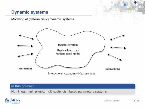
Dynamic systemsModeling of (deterministic) dynamic systems
!!!!!!!
!!!!!
!!
!!! !!!!!
!XS1! XS2!
K! F!F!
Vd1! Vd2!
M! F!
Xi1!
F! F!f!
Storage!
!Interconnection!
D
!
Dissipation!
!
!fc!
ec!
fr!
er!
ep!fp!
! !
Interactions! Interactions!Interactions:!Actuation!+!Measurement!
Dynamic!system!Physical!laws,!data!Mathematical!Model!
In this course :
Non linear, multi physic, multi scale, distributed parameters systems.
Doctoral Course 3 / 56
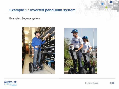
Example 1 : inverted pendulum system
Example : Segway system
Doctoral Course 4 / 56
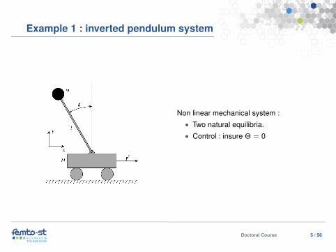
Example 1 : inverted pendulum system
Non linear mechanical system :• Two natural equilibria.• Control : insure Θ = 0
Doctoral Course 5 / 56

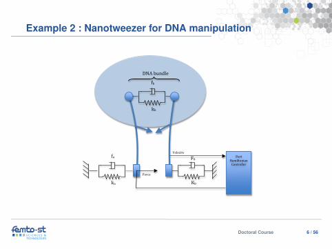
Example 2 : Nanotweezer for DNA manipulation
!! !!!
IntroductionBiocharacterizations on DNA
Control of tweezersConclusions
Single molecule techniquesSilicon nanotweezers for DNA experiments
Design of the silicon nanotweezers
[Yamahata2008]
[email protected] PhD defense (Nicolas LAFITTE) 11 / 57
Doctoral Course 6 / 56
Example 2 : Nanotweezer for DNA manipulation
!
!
"#!
$#!
$%!
"%!
&'()*!
+,-!%./01*!
2'(3!4#5613'/6#/!7'/3('11*(!
8*1')639!&%!
:%!
Doctoral Course 6 / 56
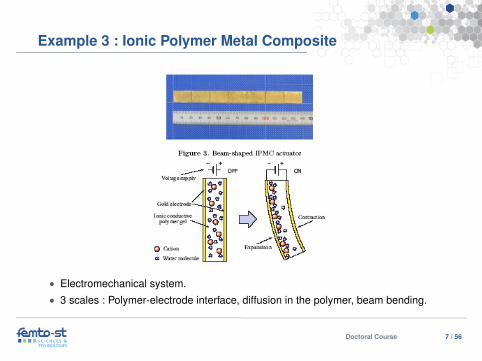
Example 3 : Ionic Polymer Metal CompositeParcours
Activitésd’enseignement
Activités derecherche
Projetsd’intégration•ENSMM•FEMTO-ST/AS2M/SAMMI
Candidature au Poste de Professeur des Universités PU 61 - 0843, 2008 ENSMM p. 15/15
! Exemple de projet support: ProjetFranco-Japonais SAKURA
! Mise en oeuvre pratique - Pilote
• Electromechanical system.• 3 scales : Polymer-electrode interface, diffusion in the polymer, beam bending.
Doctoral Course 7 / 56
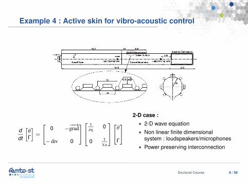
Example 4 : Active skin for vibro-acoustic control
Enfin la troisième equation est une relation thermodynamique qui relie la pres-sion à la masse volumique:
dp
dρ=
1
ρχs(3)
χs: coefficient de compressibilite adiabatique(Pa−1)
Le coefficient χs est la compressibilite adiabatique, c’est-à-dire que l’on s’interesseà des variations de pression et de la masse volumique mais sans changement detempérature.
2 Energie acoustiqueLes paramètres des equations de propagation de l’onde acoustique dans un tubecf. figure 1, vont nous permettre d’exprimer la densite d’energie acoustique quidepend à la fois du carre de la pression (energie potentielle) et du carre de lavitesse (energie cinetique).
Figure 1: Modélisation du système source, tube et membrane.
Equation de propagation faisant intervenir la pression [2, p. 118]:
ρ0χsd2p
d2t−∆p = 0 (4)
Equation de propagation faisant intervenir la vitesse vibratoire [3]:
ρ0χsd2v
d2t−∆v = 0 (5)
L’équation de propagation (en Pression) en coordonnés cartésiennes (2D):
ρ0χsd2p
d2t− d2p
d2x− d2p
d2y= 0 (6)
2
ddt
[θΓ
]=
0 −−−→grad
− div 0
1ρ0
0
0 1χs
θ
Γ
2-D case :
• 2-D wave equation• Non linear finite dimensional
system : loudspeakers/microphones• Power preserving interconnection
Doctoral Course 8 / 56
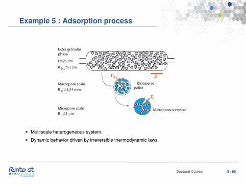
Example 5 : Adsorption process
Parcours
Activitésd’enseignement
Activités derecherche•Motivation•Développementsthéoriques
•Projets -Encadrements- Publications
Projetsd’intégration
Candidature au Poste de Professeur des Universités PU 61 - 0843, 2008 ENSMM p. 9/15
Procédé d’adsorption par modulation de pression (A. Baaiu PHD)
Objectif : séparation par adsorption
(coll. IFP)
A
B
A B
B
! Système hétérogène
multi-échelles, régi par
thermodynamique irréversible
! EDP non linéaires
Microporous crystal
Bidispersepellet
rp z
rc
L!25 cm
R !1,24 mm
R !1 µmc
p
Extra granular phase
Macropore scale
Micropore scale
R !1 cmint
• Multiscale heterogeneous system.
• Dynamic behavior driven by irreversible thermodynamic laws
Doctoral Course 9 / 56

Example 5 : Adsorption process
Parcours
Activitésd’enseignement
Activités derecherche•Motivation•Développementsthéoriques
•Projets -Encadrements- Publications
Projetsd’intégration
Candidature au Poste de Professeur des Universités PU 61 - 0843, 2008 ENSMM p. 9/15
Procédé d’adsorption par modulation de pression (A. Baaiu PHD)
Objectif : séparation par adsorption
(coll. IFP)
A
B
A B
B
! Système hétérogène
multi-échelles, régi par
thermodynamique irréversible
! EDP non linéaires
Microporous crystal
Bidispersepellet
rp z
rc
L!25 cm
R !1,24 mm
R !1 µmc
p
Extra granular phase
Macropore scale
Micropore scale
R !1 cmint
• Multiscale heterogeneous system.
• Considered phenomena :
• Fluid scale : convection, dispersion.• Pellet scale : diffusion (Stephan-Maxwell).• Microscopic scale : Knudsen law.
Doctoral Course 9 / 56
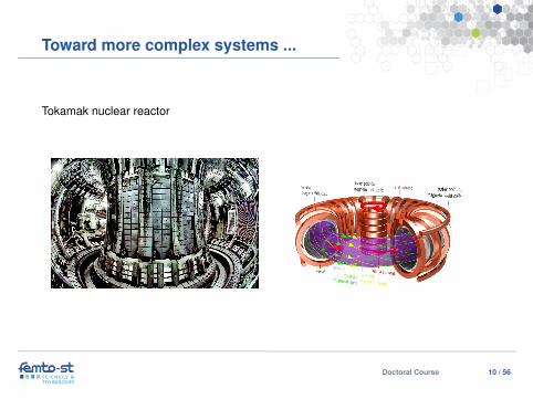
Toward more complex systems ...
Tokamak nuclear reactor
Doctoral Course 10 / 56
Models and Complexity
• A model is always an approximation of reality.• A model depends on the problem context.• A model has to be tractable.
Purpose
Derive a mathematical model based on Physics useful for :• Simulation (model reduction)• Analysis• Control design
Doctoral Course 11 / 56
Models and Complexity (illustration)
Parcours
Activitésd’enseignement
Activités derecherche•Motivation•Développementsthéoriques
•Projets -Encadrements- Publications
Projetsd’intégration
Candidature au Poste de Professeur des Universités PU 61 - 0843, 2008 ENSMM p. 9/15
Procédé d’adsorption par modulation de pression (A. Baaiu PHD)
Objectif : séparation par adsorption
(coll. IFP)
A
B
A B
B
! Système hétérogène
multi-échelles, régi par
thermodynamique irréversible
! EDP non linéaires
Microporous crystal
Bidispersepellet
rp z
rc
L!25 cm
R !1,24 mm
R !1 µmc
p
Extra granular phase
Macropore scale
Micropore scale
R !1 cmint
Remark 3.1 The Hodge star operator ! is a linear operator mapping p forms on V to (n" p)forms i.e. :
! : !p(V ) # !n!p(V )
In cartesian coordinates, consider the functions g(z) and the 1-form f(z) = g(z)dz then !f(z) =g(z). qL
s and qL being 1-forms, !qLs and !qL are 0-forms.
(3) Closure equation associated with the di!usion - We use Knudsen law [19] to presentthe di"usion in the adsorbed phase (microporous scale). That is to say we only consider thefriction exerted by the solid on the adsorbed species. So the constitutive relation representingthe di"usion is:
fmic2 = "Dmic ! qL
RT! emic
2 (15)
where Dmic is the di"usion constant.
4 Model reduction based on geometrical properties
4.1 General concept
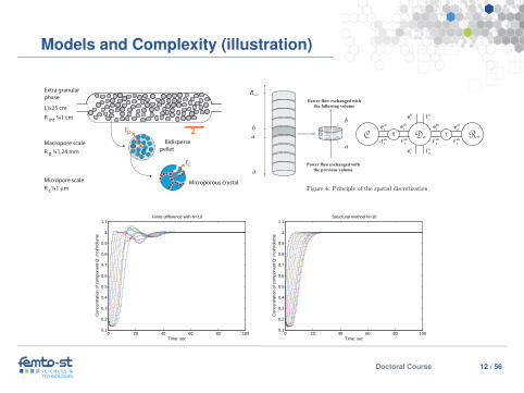
As previously mentioned, the port based modelling of the adsorption column is based on basicelements having well defined energetic behavior as already depicted in Figure 3. The dis-tributed aspect of this port based model is essentially supported by the Dirac structure whichlinks power exchanges within the spatial domain and through the boundaries. The proposeddiscretization method consists in splitting the initial structured infinite dimensional model intoN finite dimensional sub-models (finite elements) with the same energetic behavior (cf Figure 4).Furthermore, the support functions used for the interpolation of both e"ort and flow variablesare di"erent to have enough degrees of freedom to guarantee the conservation of the structuralproperties.
e1
ab
f1
ab
e2
ab
f2
ab-f
1
ab
e1
ab -e2
ab
f2
ab
e1
a
e1
b
f2
a
f2
b
DabC Rab
a b
0
Rmic
a b
Power flow exchanged with
the following volume
Power flow exchanged with the previous volume
0 1
Figure 4: Principle of the spatial discretization
The interconnection between these sub-models is done using the power conjugate boundaryport variables. They correspond to the energy flowing across the boundary of one submodel tothe boundary of the next sub-model. To each submodel is associated the same generic structure(and consequently parts of the global mass and energy balances) as the global structure, thedi"erence lying in the fact that submodels are finite dimensional i.e. the Dirac structure Dab
on Figure 4 is finite dimensional and the reduced e"ort and flow variables (eab, fab) are no morespatially distributed.
For simplicity reasons superscript mic will be omitted in the remaining of the section. Letus now explain the reduction scheme.
7
0 20 40 60 80 1000.1
0.2
0.3
0.4
0.5
0.6
0.7
0.8
0.9
1
1.1
Time: sec
Con
cent
ratio
n of
com
pone
nt Q
: mol
/Vol
ume
Finite difference with N=10
0 20 40 60 80 1000.1
0.2
0.3
0.4
0.5
0.6
0.7
0.8
0.9
1
1.1
Time: sec
Con
cent
ratio
n of
com
pone
nt Q
: mol
/Vol
ume
Structural method N=10
Doctoral Course 12 / 56

Outline
1. Dynamic systems modeling
2. Port Hamiltonian framework
3. Back to modeling
4. Port Hamiltonian modeling
Doctoral Course 13 / 56
Port Hamiltonian framework
Philosophy
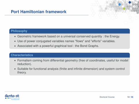
• Geometric framework based on a universal conserved quantity : the Energy.• Use of power conjugated variables names "flows" and "efforts" variables.• Associated with a powerful graphical tool : the Bond Graphs.
Characteristics
• Formalism coming from differential geometry (free of coordinates, useful for modelreduction).
• Suitable for functional analysis (finite and infinite dimension) and system controltheory.
Doctoral Course 14 / 56
Port Hamiltonian framework
Port Hamiltonian systems
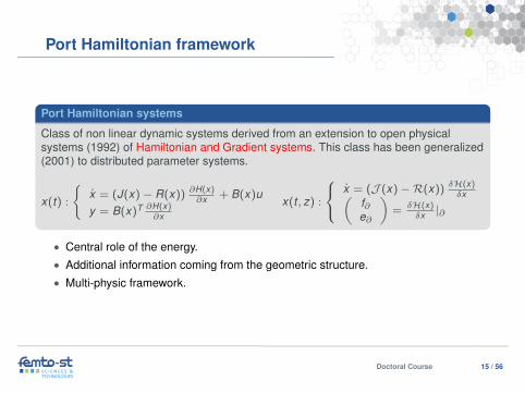
Class of non linear dynamic systems derived from an extension to open physicalsystems (1992) of Hamiltonian and Gradient systems. This class has been generalized(2001) to distributed parameter systems.
x(t) :
{x = (J(x)− R(x)) ∂H(x)
∂x + B(x)uy = B(x)T ∂H(x)
∂x
x(t , z) :
x = (J (x)−R(x)) δH(x)δx(
f∂e∂
)= δH(x)
δx |∂
• Central role of the energy.• Additional information coming from the geometric structure.• Multi-physic framework.
Doctoral Course 15 / 56
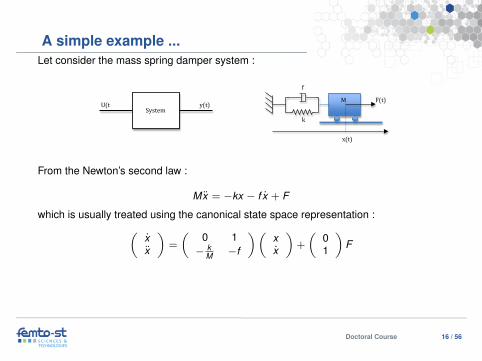
A simple example ...Let consider the mass spring damper system :!
"!
#!
$!
%&'(!
)&'(!*&'(!
+&'(!,+-'./!
From the Newton’s second law :
Mx = −kx − f x + F
which is usually treated using the canonical state space representation :(xx
)=
(0 1− k
M −f
)(xx
)+
(01
)F
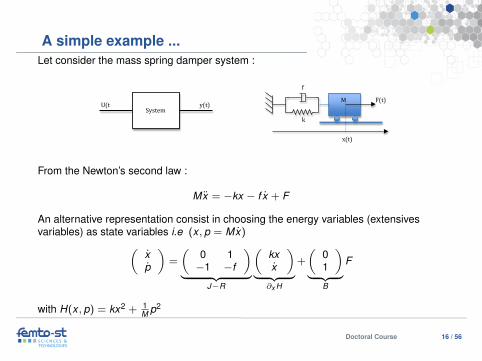
An alternative representation consist in choosing the energy variables (extensivesvariables) as state variables i.e (x , p = Mx)(
xp
)=
(0 1−1 −f
)︸ ︷︷ ︸
J−R
(kxx
)︸ ︷︷ ︸∂x H
+
(01
)︸ ︷︷ ︸
B
F
with H(x , p) = kx2 + 1M p2
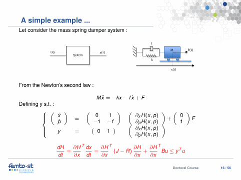
Defining y s.t. :(
xp
)=
(0 1−1 −f
) (∂x H(x , p)∂pH(x , p)
)+
(01
)F
y =(
0 1) (
∂x H(x , p)∂pH(x , p)
)dHdt
=∂H∂x
T dxdt
=∂H∂x
T(J − R)
∂H∂x
+∂H∂x
TBu ≤ yT u
Doctoral Course 16 / 56
A simple example ...Let consider the mass spring damper system :!
"!
#!
$!
%&'(!
)&'(!*&'(!
+&'(!,+-'./!
From the Newton’s second law :
Mx = −kx − f x + F
which is usually treated using the canonical state space representation :(xx
)=
(0 1− k
M −f
)(xx
)+
(01
)F
An alternative representation consist in choosing the energy variables (extensivesvariables) as state variables i.e (x , p = Mx)(
xp
)=
(0 1−1 −f
)︸ ︷︷ ︸
J−R
(kxx
)︸ ︷︷ ︸∂x H
+
(01
)︸ ︷︷ ︸
B
F
with H(x , p) = kx2 + 1M p2
Defining y s.t. :(
xp
)=
(0 1−1 −f
) (∂x H(x , p)∂pH(x , p)
)+
(01
)F
y =(
0 1) (
∂x H(x , p)∂pH(x , p)
)dHdt
=∂H∂x
T dxdt
=∂H∂x
T(J − R)
∂H∂x
+∂H∂x
TBu ≤ yT u
Doctoral Course 16 / 56

Outline
1. Dynamic systems modeling
2. Port Hamiltonian framework
3. Back to modeling
4. Port Hamiltonian modeling
Doctoral Course 17 / 56
Back to the modeling
The previous model can be written from the interconnection of a subset of basicmechanical elements :
• A moving inertia.• A spring.• A damper.• A source and some interconnection relations.
Structured modeling
Each element is characterized by a set of power conjugated variables, the flowvariables and the effort variables (intensive variables). The state variable is derive fromthe time integration of the flow variables (extensive variables). When the component ispurely dissipative there is no associated state variable.
Doctoral Course 18 / 56
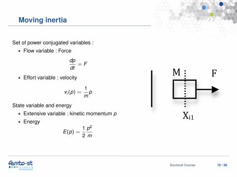
Moving inertia
Set of power conjugated variables :• Flow variable : Force
dpdt
= F
• Effort variable : velocity
vi (p) =1m
p
State variable and energy• Extensive variable : kinetic momentum p• Energy
E(p) =12
p2
m
!
!XS1! XS2!
K!
Vd1! Vd2!
M! F!
Xi1!
F! F!F!F!
f!
Doctoral Course 19 / 56
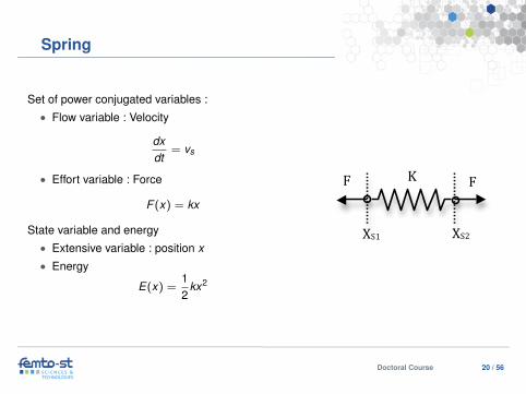
Spring
Set of power conjugated variables :• Flow variable : Velocity
dxdt
= vs
• Effort variable : Force
F (x) = kx
State variable and energy• Extensive variable : position x• Energy
E(x) =12
kx2
!
!XS1! XS2!
K!
Vd1! Vd2!
M! F!
Xi1!
F! F!F!F!
f!
Doctoral Course 20 / 56
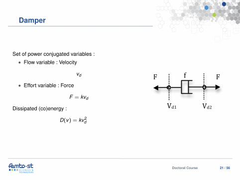
Damper
Set of power conjugated variables :• Flow variable : Velocity
vd
• Effort variable : Force
F = kvd
Dissipated (co)energy :
D(v) = kv2d
!
!XS1! XS2!
K!
Vd1! Vd2!
M! F!
Xi1!
F! F!F!F!
f!
Doctoral Course 21 / 56
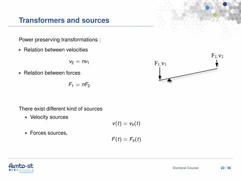
Transformers and sources
Power preserving transformations :
• Relation between velocities
v2 = nv1
• Relation between forces
F1 = nF2
!!
!
!
!!!!
!
!!
!!
!!!! !!!!!
Vd1! Vd2!
M! F!
Xi1!
F! F!f!
Storage!
!Interconnection!
D
!
Dissipation!
!
!fc!
ec!
fr!
er!
ep!fp!
! !
Interactions! Interactions!Interactions:!Actuation!+!Measurement!
Dynamic!system!Physical!laws,!data!Mathematical!Model!
!XS1! XS2!
K! F!F!
u!
R!i!
CR!
i!
u!
LR!
CR!
i! R!
e! L!
F2,!v2!F1,!v1!
There exist different kind of sources• Velocity sources
v(t) = vs(t)
• Forces sources,F (t) = Fs(t)
Doctoral Course 22 / 56
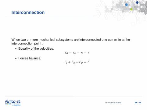
Interconnection
When two or more mechanical subsystems are interconnected one can write at theinterconnection point :
• Equality of the velocities,vd = vs = vi = v
• Forces balance,Fi + Fs + Fd = F
Doctoral Course 23 / 56
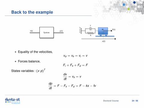
Back to the example!
"!
#!
$!
%&'(!
)&'(!*&'(!
+&'(!,+-'./!
• Equality of the velocities,vd = vs = vi = v
• Forces balance,Fi + Fs + Fd = F
States variables : (x p)T
dxdt
= vs = v
dpdt
= F − Fs − Fd = F − kx − fv
Doctoral Course 24 / 56

Outline
1. Dynamic systems modeling
2. Port Hamiltonian framework
3. Back to modeling
4. Port Hamiltonian modeling
Doctoral Course 25 / 56
Electric circuits
Coupling between electric fields and magnetic fields• Capacitors.• Inductors.• Resistors.• Transformers and sources.• Interconnection relations.
Doctoral Course 26 / 56
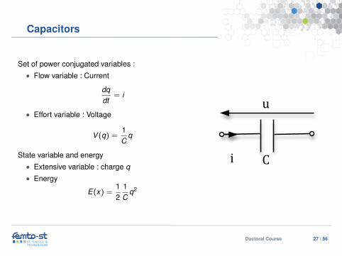
Capacitors
Set of power conjugated variables :• Flow variable : Current
dqdt
= i
• Effort variable : Voltage
V (q) =1C
q
State variable and energy• Extensive variable : charge q• Energy
E(x) =12
1C
q2
!!
!
!
!!!!
!
!!
!!
!!!! !!!!!
Vd1! Vd2!
M! F!
Xi1!
F! F!f!
Storage!
!Interconnection!
D
!
Dissipation!
!
!fc!
ec!
fr!
er!
ep!fp!
! !
Interactions! Interactions!Interactions:!Actuation!+!Measurement!
Dynamic!system!Physical!laws,!data!Mathematical!Model!
!XS1! XS2!
K! F!F!
u!
R!i!
CR!
i!
u!
LR!
i!
u,Φ!
Doctoral Course 27 / 56
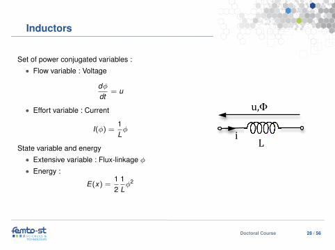
Inductors
Set of power conjugated variables :• Flow variable : Voltage
dφdt
= u
• Effort variable : Current
I(φ) =1Lφ
State variable and energy• Extensive variable : Flux-linkage φ• Energy :
E(x) =12
1Lφ2
!!
!
!
!!!!
!
!!
!!
!!!! !!!!!
Vd1! Vd2!
M! F!
Xi1!
F! F!f!
Storage!
!Interconnection!
D
!
Dissipation!
!
!fc!
ec!
fr!
er!
ep!fp!
! !
Interactions! Interactions!Interactions:!Actuation!+!Measurement!
Dynamic!system!Physical!laws,!data!Mathematical!Model!
!XS1! XS2!
K! F!F!
u!
R!i!
CR!
i!
u!
LR!
i!
u,Φ!
Doctoral Course 28 / 56
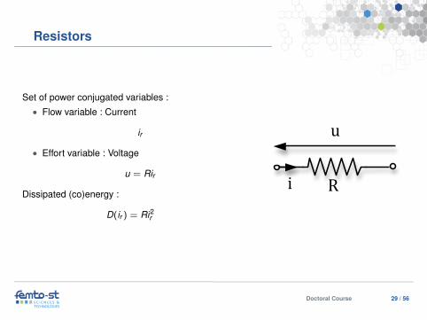
Resistors
Set of power conjugated variables :• Flow variable : Current
ir
• Effort variable : Voltage
u = Rir
Dissipated (co)energy :
D(ir ) = Ri2r
!!
!
!
!!!!
!
!!
!!
!!!! !!!!!
Vd1! Vd2!
M! F!
Xi1!
F! F!f!
Storage!
!Interconnection!
D
!
Dissipation!
!
!fc!
ec!
fr!
er!
ep!fp!
! !
Interactions! Interactions!Interactions:!Actuation!+!Measurement!
Dynamic!system!Physical!laws,!data!Mathematical!Model!
!XS1! XS2!
K! F!F!
u!
R!i!
CR!
i!
u!
LR!
i!
u,Φ!
Doctoral Course 29 / 56
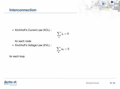
Interconnection
• Kirchhoff’s Current Law (KCL) : ∑k
ik = 0
for each node.• Kirchhoff’s Voltage Law (KVL) : ∑
k
uk = 0
for each loop.
Doctoral Course 30 / 56
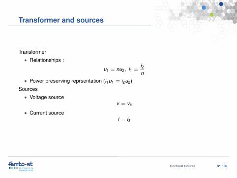
Transformer and sources
Transformer• Relationships :
u1 = nu2, i1 =i2n
• Power preserving reprsentation (i1u1 = i2u2)
Sources• Voltage source
v = vs
• Current sourcei = is
Doctoral Course 31 / 56
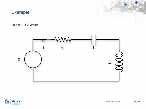
Example
Linear RLC Circuit
!!
!
!
!!!!
!
!!
!!
!!!! !!!!!
Vd1! Vd2!
M! F!
Xi1!
F! F!f!
Storage!
!Interconnection!
D
!
Dissipation!
!
!fc!
ec!
fr!
er!
ep!fp!
! !
Interactions! Interactions!Interactions:!Actuation!+!Measurement!
Dynamic!system!Physical!laws,!data!Mathematical!Model!
!XS1! XS2!
K! F!F!
u!
R!i!
CR!
i!
u!
LR!
CR!
i! R!
e! L!
Doctoral Course 32 / 56
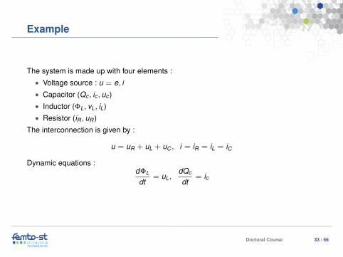
Example
The system is made up with four elements :• Voltage source : u = e, i• Capacitor (Qc , ic , uc )• Inductor (ΦL, vL, iL)• Resistor (iR , uR )
The interconnection is given by :
u = uR + uL + uC , i = iR = iL = iC
Dynamic equations :dΦL
dt= uL,
dQc
dt= ic
Doctoral Course 33 / 56

Example
Port Hamiltonian formulation. The dynamics is given by
ddt
(QcΦL
)=
(0 1−1 −R
)( 1C Qc1L ΦL
)+
(01
)u
with output mapping :
i =(
0 1)( 1
C Qc1L ΦL
)
The energy is given by E = 12
(1C Q2
c + 1L Φ2
L
)with balance
dEdt
= uT i − Ri2
Doctoral Course 34 / 56
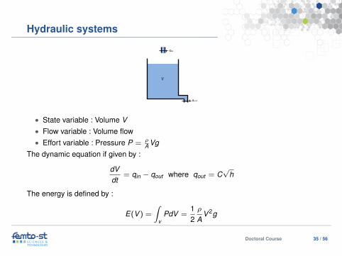
Hydraulic systems!
qin!
qout!
V!
• State variable : Volume V• Flow variable : Volume flow• Effort variable : Pressure P = ρ
A VgThe dynamic equation if given by :
dVdt
= qin − qout where qout = C√
h
The energy is defined by :
E(V ) =
∫v
PdV =12ρ
AV 2g
Doctoral Course 35 / 56
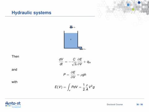
Hydraulic systems
!qin!
qout!
V!
ThendVdt
= −C√
h
∂E∂V
+ qin
andP =
∂E∂V
= ρgh
withE(V ) =
∫v
PdV =12ρ
AV 2g
Doctoral Course 36 / 56

Outline
1. Dynamic systems modeling
2. Port Hamiltonian framework
3. Back to modeling
4. Port Hamiltonian modeling
Doctoral Course 37 / 56
Port based modeling of physical systems
Port Hamiltonian formulation
The idea is to generalize what has been proposed for mechanical and electricalsystems to other class of systems.
Why ?• We have pointed out some common properties : storage, dissipation and
transformation.• Engineering systems are a combination of subsystems related to possible
different physical domains and interconnection has to be consistent. See forexample Adsorption processes.
• Decomposition in basic elements helps in modeling of complex dynamic systems(coming from different areas).
• Modeling is attached to the notion of graph.
Doctoral Course 38 / 56
Port based modeling of physical systems
Much more fundamental reasons :
• Central role of the energycan be used for control purposes. Lyapunov basedapproaches.
• More information are taken into account in the model through symmetries.
• The model is a knowledge based model that takes the non linearities and thedistributed aspects into account.
Doctoral Course 39 / 56
Generalized Bond Graph
Decomposition in basic elements is linked to Generalized Bond Graph (Paytner,Breedveld) :
• Systems are decomposed in elements with specific energetic behavior : storage,dissipation and transformation.
• Each element is characterized by a pair of power conjugated variables : the flowvariables f ∈ F and the effort variables e ∈ E . The associated power port is givenby :
P = f T e
Doctoral Course 40 / 56
Port based modeling
!
!XS1! XS2!
K! F!F!
Vd1! Vd2!
M! F!
Xi1!
F! F!f!
Storage!
!Interconnection!
D
!
Dissipation!
!
!fc!
ec!
fr!
er!
ep!fp!
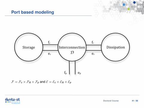
F = Fc ×FR ×Fp and E = Ec × ER × Ep
Doctoral Course 41 / 56
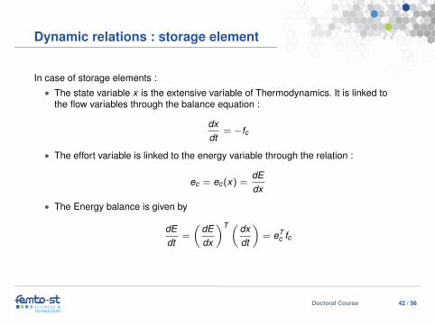
Dynamic relations : storage element
In case of storage elements :• The state variable x is the extensive variable of Thermodynamics. It is linked to
the flow variables through the balance equation :
dxdt
= −fc
• The effort variable is linked to the energy variable through the relation :
ec = ec(x) =dEdx
• The Energy balance is given by
dEdt
=
(dEdx
)T (dxdt
)= eT
c fc
Doctoral Course 42 / 56
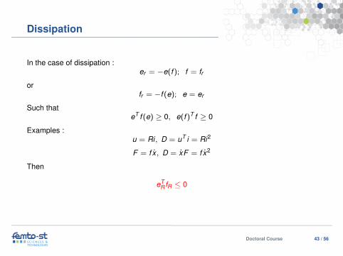
Dissipation
In the case of dissipation :er = −e(f ); f = fr
orfr = −f (e); e = er
Such thateT f (e) ≥ 0, e(f )T f ≥ 0
Examples :u = Ri, D = uT i = Ri2
F = f x , D = xF = f x2
Then
eTR fR ≤ 0
Doctoral Course 43 / 56
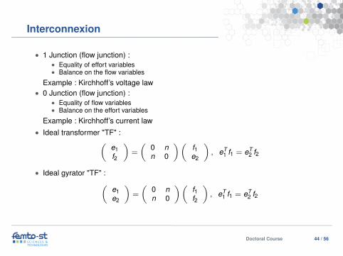
Interconnexion
• 1 Junction (flow junction) :• Equality of effort variables• Balance on the flow variables
Example : Kirchhoff’s voltage law• 0 Junction (flow junction) :
• Equality of flow variables• Balance on the effort variables
Example : Kirchhoff’s current law• Ideal transformer "TF" :(
e1f2
)=
(0 nn 0
)(f1e2
), eT
1 f1 = eT2 f2
• Ideal gyrator "TF" :(e1e2
)=
(0 nn 0
)(f1f2
), eT
1 f1 = eT2 f2
Doctoral Course 44 / 56
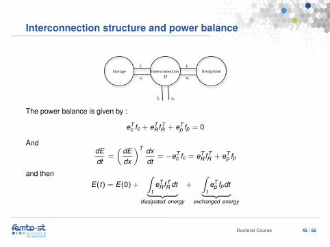
Interconnection structure and power balance
!
!XS1! XS2!
K! F!F!
Vd1! Vd2!
M! F!
Xi1!
F! F!f!
Storage!
!Interconnection!
D
!
Dissipation!
!
!fc!
ec!
fr!
er!
ep!fp!
The power balance is given by :
eTc fc + eT
R f TR + eT
p fp = 0
AnddEdt
=
(dEdx
)T dxdt
= −eTc fc = eT
R f TR + eT
p fp
and thenE(t) = E(0) +
∫teT
R f TR dt︸ ︷︷ ︸
dissipated energy
+
∫teT
p fpdt︸ ︷︷ ︸exchanged energy
Doctoral Course 45 / 56
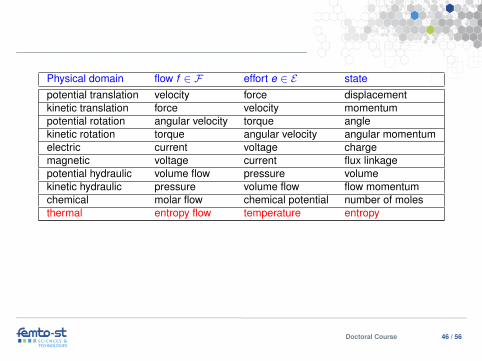
Physical domain flow f ∈ F effort e ∈ E statepotential translation velocity force displacementkinetic translation force velocity momentumpotential rotation angular velocity torque anglekinetic rotation torque angular velocity angular momentumelectric current voltage chargemagnetic voltage current flux linkagepotential hydraulic volume flow pressure volumekinetic hydraulic pressure volume flow flow momentumchemical molar flow chemical potential number of molesthermal entropy flow temperature entropy
Doctoral Course 46 / 56
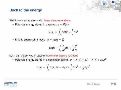
Back to the energy
Well known subsystems with linear closure relations• Potential energy stored in a spring : e = F (x)
E(x) =
∫x
Kxdx =12
Kx2
• Kinetic energy oh a mass : e = v(p) = pM
E(p) =
∫p
pM
dp =12
p2
M
but it can be derived in case of non linear closure relations• Potential energy stored in a non linear spring : e = K (x) = K0 + K1X + K2X 2
E(x) =
∫x
K (x)dx = K0x +12
K1x2 +13
K2x3
Doctoral Course 47 / 56
Energy and co energy
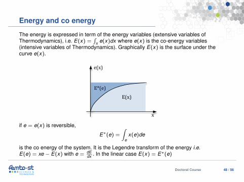
The energy is expressed in term of the energy variables (extensive variables ofThermodynamics), i.e. E(x) =
∫x e(x)dx where e(x) is the co-energy variables
(intensive variables of Thermodynamics). Graphically E(x) is the surface under thecurve e(x).
!
e(x)!
x!
E(x)!E*(e)!
if e = e(x) is reversible,
E∗(e) =
∫e
x(e)de
is the co energy of the system. It is the Legendre transform of the energy i.e.E(e) = xe − E(x) with e = dE
dx . In the linear case E(x) = E∗(e)
Doctoral Course 48 / 56
Energy and co energy
In the case of moving inertia :• Effort variable e = v• State variable p
Or p = Mv then
E(p) =
∫v
p(v)dv =12
Mv2
In this case the Legendre transform of the energy is given by
E∗(v) = pv − E(p) = pv −12
Mv2 =12
Mv2 = E(p)
Doctoral Course 49 / 56
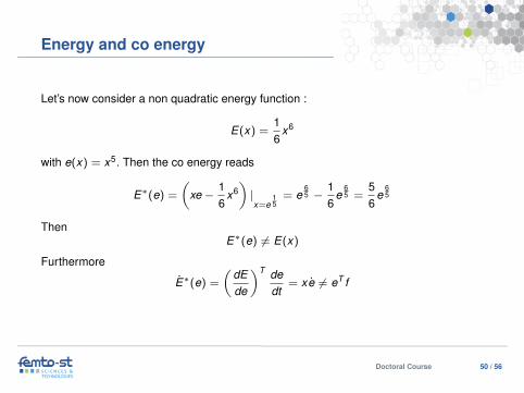
Energy and co energy
Let’s now consider a non quadratic energy function :
E(x) =16
x6
with e(x) = x5. Then the co energy reads
E∗(e) =
(xe −
16
x6)|x=e
15
= e65 −
16
e65 =
56
e65
ThenE∗(e) 6= E(x)
Furthermore
E∗(e) =
(dEde
)T dedt
= xe 6= eT f
Doctoral Course 50 / 56
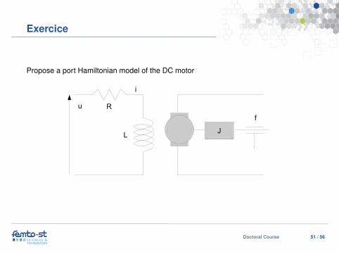
Exercice
Propose a port Hamiltonian model of the DC motor
J
R
L
f
u
i
Doctoral Course 51 / 56
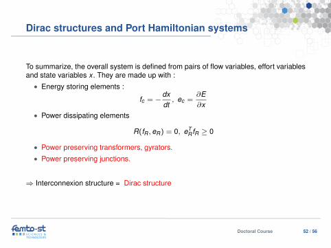
Dirac structures and Port Hamiltonian systems
To summarize, the overall system is defined from pairs of flow variables, effort variablesand state variables x . They are made up with :
• Energy storing elements :
fc = −dxdt, ec =
∂E∂x
• Power dissipating elements
R(fR , eR) = 0, eTR fR ≥ 0
• Power preserving transformers, gyrators.• Power preserving junctions.
⇒ Interconnexion structure = Dirac structure
Doctoral Course 52 / 56
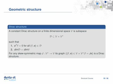
Geometric structure
Dirac structure
A constant Dirac structure on a finite dimensional space V is subspace
D ⊂ V × V∗
such that
1. eT f = 0 for all (f , e) ∈ D2. dimD = dimV
For any skew-symmetric map J : V∗ → V its graph {(f , e) ∈ V × V∗|f = Je} is a Diracstructure.
Doctoral Course 53 / 56
Geometric structure
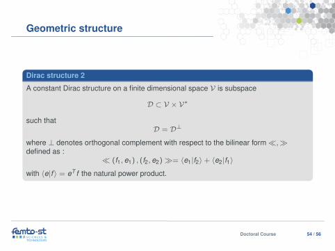
Dirac structure 2
A constant Dirac structure on a finite dimensional space V is subspace
D ⊂ V × V∗
such thatD = D⊥
where ⊥ denotes orthogonal complement with respect to the bilinear form�,�defined as :
� (f1, e1) , (f2, e2)�= 〈e1|f2〉+ 〈e2|f1〉
with 〈e|f 〉 = eT f the natural power product.
Doctoral Course 54 / 56
Geometric structure
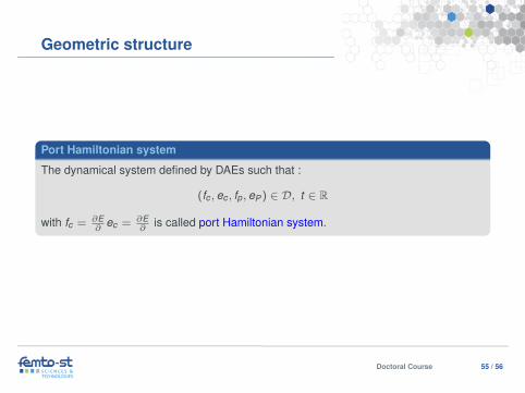
Port Hamiltonian system
The dynamical system defined by DAEs such that :
(fc , ec , fp, eP) ∈ D, t ∈ R
with fc = ∂E∂
ec = ∂E∂
is called port Hamiltonian system.
Doctoral Course 55 / 56

Doctoral Course 56 / 56