1

SLAM – Landmark-based FastSLAM

Introduction to Mobile Robotics

Partial slide courtesy of Mike Montemerlo

Marina Kollmitz, Wolfram Burgard

2

SLAM stands for simultaneous localization and mapping

The task of building a map while estimating the pose of the robot relative to this map

Why is SLAM hard? Chicken-or-egg problem: A map is needed to localize the robot A pose estimate is needed to build a map

The SLAM Problem

3

Given: The robot’s

controls Observations of

nearby features

Estimate: Map of features Path of the robot

The SLAM Problem A robot moving through an unknown, static environment

4

Typical models are: Feature maps Grid maps (occupancy or reflection

probability maps)

Map Representations

5

Why is SLAM a Hard Problem?

SLAM: robot path and map are both unknown!

Robot path error correlates errors in the map

7

Why is SLAM a Hard Problem?

In the real world, the mapping between observations and landmarks is unknown

Picking wrong data associations can have catastrophic consequences

Pose error correlates data associations

Robot pose uncertainty

9

Data Association Problem

A data association is an assignment of observations to landmarks

In general there are more than (n observations, m landmarks) possible associations

Also called “assignment problem”

Particle Filters Represent belief by random samples Estimation of non-Gaussian, nonlinear

processes

Sampling Importance Resampling (SIR) principle Draw the new generation of particles Assign an importance weight to each particle Resample

Typical application scenarios are tracking,

localization, …

10

Recap: Particle Filter Localization

11

1. initialize particles 2. apply motion

model 3. weight particles

(sensor model) 4. resample

according to weight

Recap: Particle Filter Localization

12

1. initialize particles 2. apply motion

model 3. weight particles

(sensor model) 4. resample

according to weight

Recap: Particle Filter Localization

13

1. initialize particles 2. apply motion

model 3. weight particles

(sensor model) 4. resample

according to weight

Recap: Particle Filter Localization

14

1. initialize particles 2. apply motion

model 3. weight particles

(sensor model) 4. resample

according to weight

Actual measurement:

Recap: Particle Filter Localization

15

1. initialize particles 2. apply motion

model 3. weight particles

(sensor model) 4. resample

according to weight

1 2

1

2

1

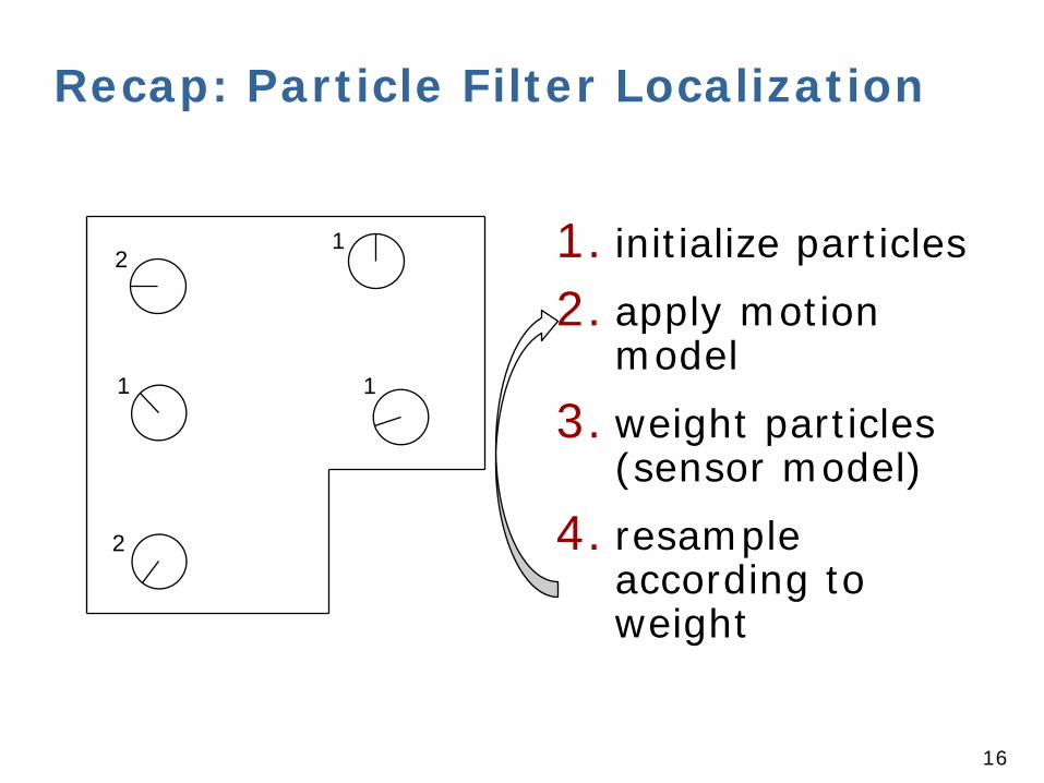
Recap: Particle Filter Localization

16

1. initialize particles 2. apply motion

model 3. weight particles

(sensor model) 4. resample

according to weight

1 2

1

2

1

Localization vs. SLAM A particle filter can be used to solve both

problems Localization: state space <x, y, θ> SLAM: state space <x, y, θ, map> for landmark maps = <l1, l2, …, lm> for grid maps = <c11, c12, …, c1n, c21, …, cnm>

Problem: The number of particles needed to

represent a posterior grows exponentially with the dimension of the state space!

17

Dependencies Is there a dependency between certain

dimensions of the state space? If so, can we use the dependency to solve

the problem more efficiently?

In the SLAM context The map depends on the poses of the robot. We know how to build a map given the position

of the sensor is known.

18

Rao-Blackwellization Factorization to exploit dependencies

between variables:

If can be computed in closed form, represent only with samples and compute for every sample

It comes from the Rao-Blackwell theorem

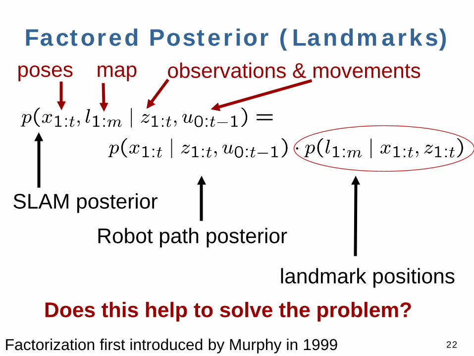
Factored Posterior (Landmarks)

20 Factorization first introduced by Murphy in 1999

poses map observations & movements

Factored Posterior (Landmarks)

21 Factorization first introduced by Murphy in 1999

poses map observations & movements

Factored Posterior (Landmarks)

22

SLAM posterior Robot path posterior

landmark positions

Factorization first introduced by Murphy in 1999

Does this help to solve the problem?

poses map observations & movements

Revisit the Graphical Model

Courtesy: Thrun, Burgard, Fox

Revisit the Graphical Model known

Courtesy: Thrun, Burgard, Fox

Landmarks are Conditionally Independent Given the Poses

Landmark variables are all disconnected (i.e. independent) given the robot’s path

26

Remember: Landmarks Correlated

SLAM: robot path and map are both unknown!

Robot path error correlates errors in the map

27

After Factorization

For estimating landmarks: robot path known!

Landmarks are not correlated

31

Factored Posterior

Robot path posterior (localization problem) Conditionally

independent landmark positions

32

Rao-Blackwellization for SLAM

Given that the second term can be computed

efficiently, particle filtering becomes possible!

33

FastSLAM Rao-Blackwellized particle filtering based on

landmarks [Montemerlo et al., 2002] Each landmark is represented by a 2x2

Extended Kalman Filter (EKF) Each particle therefore has to maintain M EKFs

Landmark 1 Landmark 2 Landmark M … x, y, θ

Landmark 1 Landmark 2 Landmark M … x, y, θ Particle #1

Landmark 1 Landmark 2 Landmark M … x, y, θ Particle #2

Particle N

…

34

FastSLAM – Action Update

Particle #1

Particle #2

Particle #3

Landmark #1 Filter

Landmark #2 Filter

35

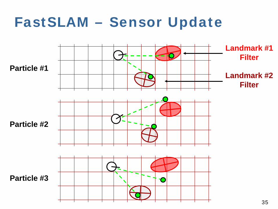
FastSLAM – Sensor Update

Particle #1

Particle #2

Particle #3

Landmark #1 Filter

Landmark #2 Filter

36

FastSLAM – Sensor Update

Particle #1

Particle #2

Particle #3

Weight = 0.8

Weight = 0.4

Weight = 0.1

37

FastSLAM – Sensor Update

Particle #1

Particle #2

Particle #3

Update map of particle #1

Update map of particle #2

Update map of particle #3

38

FastSLAM - Video

FastSLAM Complexity – Naive Update robot particles

based on the control

Incorporate an observation into the Kalman filters (given the data association)

Resample particle set

N = Number of particles M = Number of map features

O(N)

O(N)

O(N M)

A Better Data Structure for FastSLAM

Courtesy: M. Montemerlo

A Better Data Structure for FastSLAM

5 7

FastSLAM Complexity Update robot particles

based on the control

Incorporate an observation into the Kalman filters (given the data association)

Resample particle set

N = Number of particles M = Number of map features O(N log(M))

43

Data Association Problem

A robust SLAM solution must consider possible data associations

Potential data associations depend also on the pose of the robot

Which observation belongs to which landmark?

44

Multi-Hypothesis Data Association

Data association is done on a per-particle basis

Robot pose error is factored out of data association decisions

45

Per-Particle Data Association

Was the observation generated by the red or the brown landmark?

P(observation|red) = 0.3 P(observation|brown) = 0.7

Two options for per-particle data association Pick the most probable match Pick a random association weighted by

the observation likelihoods If the probability is too low, generate a new

landmark

46

Results – Victoria Park

4 km traverse < 5 m RMS

position error 100 particles

Dataset courtesy of University of Sydney

Blue = GPS Yellow = FastSLAM

47

Results – Victoria Park (Video)

Dataset courtesy of University of Sydney

48

Results – Data Association

49

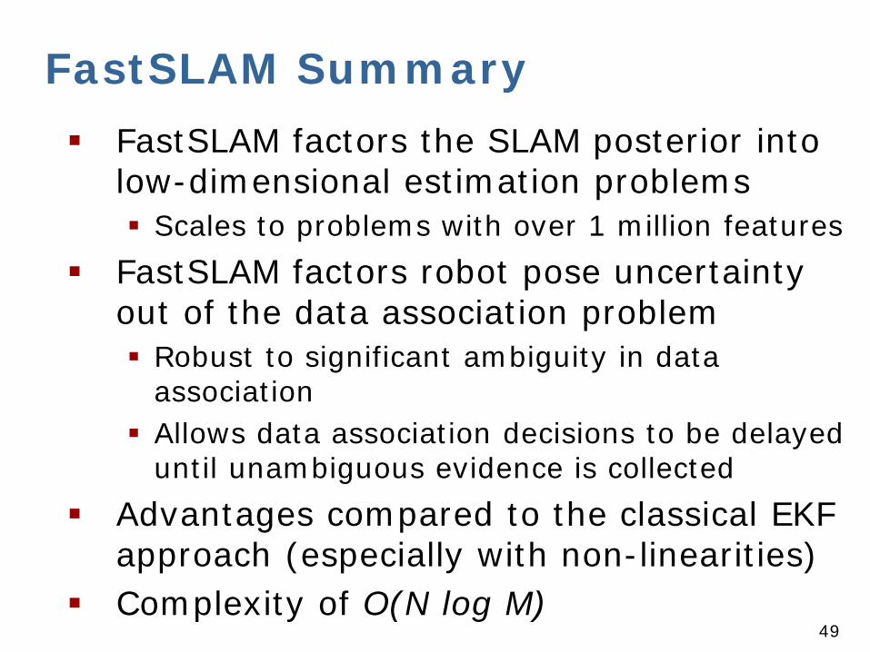
FastSLAM Summary FastSLAM factors the SLAM posterior into

low-dimensional estimation problems Scales to problems with over 1 million features

FastSLAM factors robot pose uncertainty out of the data association problem Robust to significant ambiguity in data

association Allows data association decisions to be delayed

until unambiguous evidence is collected Advantages compared to the classical EKF

approach (especially with non-linearities) Complexity of O(N log M)