FastSLAM with Stereo VisionWikus Brink

Electronic Systems LabElectrical and Electronic Engineering

Stellenbosch UniversityEmail: wikusbrink@ieee.org

Corne E. van DaalenElectronic Systems Lab

Electrical and Electronic EngineeringStellenbosch University

Email: cvdaalen@sun.ac.za

Willie BrinkApplied Mathematics

Department of Mathematical SciencesStellenbosch University

Email: wbrink@sun.ac.za

Abstract—We consider the problem of performing simultane-ous localization and mapping (SLAM) with a stereo vision sensor,where image features are matched and triangulated for use aslandmarks. We explain how we obtain landmark measurementsfrom image features, and describe them with a Gaussian noisemodel for use with a Rao-Blackwellized particle filter-basedSLAM algorithm called FastSLAM. This algorithm uses particlesto describe uncertainty in robot pose, and Gaussian distributionsto describe landmark position estimates. Simulation and experi-mental results indicate that FastSLAM is well suited for vision-based SLAM, because of an inherent robustness to landmarkmismatches, and we achieve accuracies that are comparable toother state-of-the-art systems.

I. INTRODUCTION

Simultaneous localization and mapping (SLAM) is a rapidlygrowing part of the autonomous navigation field. SLAMattempts to solve the problem of estimating a mobile robot’sposition in an unknown environment while building a mapof the environment at the same time. This is a challengingproblem since an accurate map is necessary for localizationand accurate localization is necessary for mapping.

Most SLAM algorithms use a probabilistic landmark-basedmap rather than a dense map. If landmarks in the map canbe measured, relative to the robot, and tracked over time thepose of the robot and the locations of the landmarks can beestimated in an optimal manner.

Initial implementations made use of the extended Kalmanfilter (EKF), but displayed several shortcomings such asquadratic complexity and sensitivity to incorrect feature track-ing [1] [2]. The particle filter can be used to overcome theselimitations. However, because of the high dimensionality ofthe problem the particle filter cannot be used directly. Instead,the Rao-Blackwellized particle filter [3] is used. This filterestimates some states with particles and others with EKFs.In the case of SLAM particles are used for the pose of therobot and an EKF for each landmark. This method is calledFastSLAM and has shown promising results in the literature[4] [5].

Stereo vision is an attractive sensor to use with SLAM asit can provide a large amount of 3D information at everytime step. Extracting that information reliably can, however,be challenging. Powerful algorithms such as SIFT [6] or SURF[7] have been used to solve this problem by extracting salientfeatures from images. These algorithms can be employed to

track features over multiple images so that landmarks forSLAM can be identified.

In this paper we attempt to solve the 2D SLAM problem byusing FastSLAM and image features (the 3D extension is con-ceptually the same). We begin with a brief description of howwe obtain measurements of landmarks with a Gaussian noisemodel. A detailed description of the FastSLAM algorithmis given, followed by some simulations where we compareFastSLAM with the popular EKF SLAM algorithm [2]. Weprovide experimental results from our system on an outdoordataset and measure accuracy against differential GPS groundtruth.

II. IMAGE FEATURES AND STEREO GEOMETRY

In this section we discuss a method of finding features inimages, triangulating these features for use as landmarks andapproximating the noise associated with each measurement ofa landmark. This characterization of the stereo vision sensoris important for accurate optimal estimation. Since this sectionis similar to previous work, the explanation will be brief. Fora more in depth discussion refer to [8] and [9].

A. Feature detection and matching

In order to identify landmarks we opt for one of two popularfeature detection algorithms: the scale-invariant feature trans-form (SIFT) [6] or speeded-up robust features (SURF) [7].Note that since we perform SLAM in 2D we discard thevertical coordinates of image features.

At every time step we search for feature matches in asynchronized pair of rectified stereo images. We model eachmatch as a measurement with Gaussian noise:

zim =

[xLxR

]+N (0,Nt), (1)

where xL and xR are the image coordinates of the feature inthe left and right images. By N (0,Nt) we mean a sampledrawn from the normal distribution with zero mean andcovariance matrix Nt (the same notation is used throughoutthe rest of this paper). We describe the noise covariance inEquation 1 by

Nt =

[σ2xL

00 σ2

xR

], (2)

with σxLand σxR

the standard deviations in pixels of thematch measurement, which we obtain through testing.

yrxr zr

(xL, yL)

(xR, yR)cL

cR Yw

Xw

Yr

Xr

yr

xr

ψt

?

(xt, yt)

(a) camera geometry (b) robot geometry

Fig. 1. The geometry of our system.

We can then match the descriptors of a new measurementwith the descriptors of features already found at previous timesteps, to arrive at putative landmark correspondences.

B. Stereo geometry of calibrated images

Now that we have stereo image features that can be trackedover time, we convert them into 2D landmarks.

Figure 1(a) depicts the geometry of a pair of stereo cameraswith camera centres at cL and cR, where the image planeshave been rectified, and a landmark

[xr yr zr

]Tobserved

at image coordinates (xL, yL) in the left image and (xR, yR)in the right image. As mentioned we are working in 2D, sothe features are effectively projected onto the Xr − Yr plane.

With the geometry of the stereo camera pair, the landmarklocation in metres can be calculated in robot coordinates as[

xryr

]=

[fb

xL−xR

(xL−px)bxL−xR

− b2

]+N (0,Qt), (3)

where b is the baseline (distance between cL and cR), f thefocal length and px and py the x- and y-offset of the principalpoint, all obtained from an offline calibration process. Qt isthe noise covariance matrix of the measurement.

Note that we differentiate between robot coordinates (sub-script r) and world coordinates (subscript w) as indicated inFigure 1(b), where xt, yt and ψt are the robot’s position andorientation in world coordinates at time t.

We know that a transformation from Nt to Qt is possibleif we have a linear system and, since Equation 3 is notlinear, we use a first order Taylor approximation to find thetransformation matrix

Wt =

[∂xr

∂xL

∂xr

∂xR

∂yr

∂xL

∂yr

∂xR

]. (4)

It then follows that Qt can be approximated as

Qt = WtNtWTt . (5)

This approximation is performed to maintain a Gaussian noisemodel, which is necessary for FastSLAM. We use this noisemodel and the triangulated locations of landmarks to find out-liers in putative correspondences between new measurementsand those already in the map, according to the RANSAC-basedprobabilistic method discussed in [9].

From Figure 1(b) we see that the robot pose can bedescribed with the state vector

xt =

xtytψt

, (6)

with xt and yt the location of the robot and ψt its orientation.We define the rotation matrix

Rt =

[cos(ψt) − sin(ψt)sin(ψt) cos(ψt)

]. (7)

In order to perform SLAM we need to establish a relationshipbetween robot and world coordinates. We denote the locationof a landmark i in the map corresponding with measurementj at time t as

mi,t =

[xwyw

]and zj,t =

[xryr

]. (8)

The measurement zj,t will always be as the robot observesthe landmark in robot coordinates, and the landmark’s locationmi,t will always be given in world coordinates. The transfor-mation between robot and world coordinates is given by themeasurement equation

zj,t = h(xt,mi,t) = RTt

[xw − xtyw − yt

], (9)

or inversely,

mi,t = h−1(xt, zj,t) = Rt

[xryr

]+

[xtyt

]. (10)

Exactly which measurement corresponds to which landmarkin the map, as matched with the feature descriptors andconfirmed with the outlier detection scheme, is stored in acorrespondence vector ct.

III. MOTION MODEL

Now that we have established a measurement equation, weneed to derive a motion model for our robot so that we canperform SLAM. We use the velocity motion model. At everytime step the controller of the robot will give it a forward andangular velocity,

ut =

[v

ψ

]+N (0,Mt), (11)

with v the forward translational speed and ψ the angularvelocity. To characterize the uncertainty we add zero meanGaussian noise with covariance matrix

Mt =

[α1v

2 + α2ψ2 0

0 α3v2 + α4ψ

2

], (12)

as is common practice [1]. The α parameters are robot andenvironment specific, and have to be estimated with practicaltesting and some degree of guesswork.

To update the robot states with the control input we definethe motion equation as

xt = g(xt−1,ut) =

xt−1yt−1ψt−1

+

Rt−1

[vT cos(ψT )

vT sin(ψT )

]ψT

,(13)

with T the sample period of the system. Although this is anapproximation, the accuracy lost due to the approximation isfar smaller than the effect of expected noise in the controlinput ut.

IV. SLAM WITH THE RAO-BLACKWELLIZED PARTICLEFILTER

The particle filter can be used to approximate any distri-bution, and it is often utilized to accurately estimate non-Gaussian systems. A major drawback of the particle filter,however, is that with high dimensional problems a largenumber of particles is needed to describe the distributionsufficiently. The Rao-Blackwellized particle filter has beendeveloped to overcome this problem [3]. This filter usesparticles to describe some states and Gaussian distributionsto represent all other states. In order to utilize it we need tofactorize the SLAM problem as

p(xt,m | z1:t,u1:t) = p(xt | z1:t,u1:t)

n∏i=1

p(mi | z1:t,u1:t).

(14)With this factorization we describe the required posterior asa product of n+ 1 probabilities. If we suppose that the exactlocation of the robot is known, it is reasonable to assume thatthe landmark positions are independent from one another andcan therefore be estimated independently. Naturally, we donot know the robot’s location, but this independence can beutilized when we use particles to estimate the robot position.It can even be shown that the above factorization is exact andnot an approximation [4].

FastSLAM uses a particle filter to compute the posteriorover robot states, p(xt | z1:t,u1:t), and a separate EKF forevery landmark in the map to obtain p(mi | z1:t,u1:t). Whatthis means is that, instead of only one filter, we factor theproblem into 1 + nm filters, where m is the number ofparticles. The large number of filters may seem excessive, butbecause of the low dimensionality of each individual filter thealgorithm is remarkably efficient.

We define every particle to have a state vector for the robotstates, and a mean vector and covariance matrix for everylandmark, as

Y[k]t =

⟨x[k]t ,⟨m

[k]1,t,Σ

[k]1,t

⟩, . . . ,

⟨m

[k]n,t,Σ

[k]n,t

⟩⟩, (15)

with x[k]t the robot location and orientation for particle k,

and⟨m

[k]i,t ,Σ

[k]i,t

⟩the i-th landmark’s Gaussian mean and

covariance. The FastSLAM algorithm, as it is executed atevery time step, is given below in Algorithm 1. We proceedwith a step by step explanation.

Algorithm 1 FastSLAM(Yt−1,ut, zt, ct)1: for all particles k ∈ {1, 2, . . . ,m} do

2: x[k]t ∼ p(xt |x[k]

t−1,ut)

3: for all observed landmarks zi,t do

4: j = ci,t

5: if landmark j has never been seen then

6: m[k]j,t = h−1(x

[k]t , zi,t)

7: Hj = Jh(m[k]j,t)

8: Σ[k]j,t = (H−1j )Qi(H

−1j )T

9: else

10: z = h(x[k]t ,m

[k]j,t)

11: Hj = Jh(m[k]j,t)

12: Q = HΣ[k]j,t−1H

T + Qi

13: K = Σ[k]j,t−1H

Tj Q−1

14: m[k]j,t = m

[k]j,t−1 + K(zi,t − z)

15: Σ[k]j,t = (I−KHj)Σ

[k]j,t−1

16: w[k] = w[k]f(Q, zi,t, z)

17: end if

18: end for

19: for all other landmarks j′ 6∈ ct do

20: m[k]j′,t = m

[k]j′,t−1

21: Σ[k]j′,t = Σ

[k]j′,t−1

22: end for

23: end for

24: for all k ∈ {1, 2, . . . ,m} do

25: draw random particle k with probability ∝ w[k]

26: include⟨x[k]t ,⟨m

[k]1,t,Σ

[k]1,t

⟩, . . . ,

⟨m

[k]n,t,Σ

[k]n,t

⟩⟩in Yt

27: end for

28: return Yt

• Lines 1 and 2: As with a normal particle filter, theFastSLAM algorithm begins by entering a loop over allthe particles. The control input is used to sample a newrobot pose for every particle according to the uncertaintyin the motion model. We add random noise drawn froma zero mean Gaussian distribution with a covariance ofMt, given in Equation 12, to the control input and usethe motion equation g, given in Equation 13, to find thenew location and orientation of each particle.

• Lines 3 and 4: For every particle we enter a loop over allthe measured landmarks. For every iteration the algorithmcan do one of two things: add a new landmark, or update

an old landmark. The index of an old landmark in themap is given by the correspondence vector.

• Lines 5 to 8: A new landmark is added to the mapusing the measurement equation h, given in Equation 9,to calculate its location in world coordinates. Since wewant to use an EKF to estimate each landmark we haveto linearize the measurement model by using a first orderTaylor approximation with the Jacobian

Jh(xt,mj,t) =

∂xr

∂xw

∂xr

∂yw

∂xr

∂zw∂yr

∂xw

∂yr

∂yw

∂yr

∂zw∂zr∂xw

∂zr∂yw

∂zr∂zw

. (16)

With this Jacobian we transform the uncertainty in mea-surement to an uncertainty in world coordinates.

• Lines 9 to 15: If a landmark has been observed before,we use the normal EKF equations to update its statevector and covariance. The state estimate is calculated byusing the measurement model. The measurement modelis then linearized with a Jacobian similar to the one usedfor new landmarks.

• Line 16: Once the landmark has been updated by usingthe measurement we have to calculate its effect on theweighting of the particle in question. As with a normalparticle filter the importance weight is given by

w[k] =target distribution

proposal distribution. (17)

The weighting function used in the algorithm can beshown [4] to be

f(Q, zi,t, z) = |Q|−12 e−

12 (zi,t−z)TQ−1(zi,t−z). (18)

It is not necessary to update the weight for new landmarksas they will be the same for all particles, and thereforehave no overall effect.

• Lines 19 to 22: If a previously observed feature has notbeen observed at the current time step its state vectorand uncertainty will remain unchanged. All unobservedlandmarks are therefore essentially ignored. This propertyof the algorithm is especially useful when a large mapis maintained, as the number of unseen landmarks in themap does not impact the execution time.

• Lines 24 to 27: Resampling is done by drawing parti-cles with a probability proportional to their normalizedweights. Particles with low weights will be more likelyto perish while particles with high weights will be copiedand used at the next time step.

• Line 28: Finally the updated and resampled particles arereturned to be used at the next time step.

A powerful possibility emerging from the use of particlesis that of multiple hypothesis tracking. What it entails is that,since particles represent possible paths that the robot couldhave taken, we can calculate landmark correspondences foreach particle separately. Because of the expensive nature ofcalculating feature matches we decide against this procedureand, instead, calculate one correspondence vector for all the

particles. It is, however, important to note that the algorithmcreates this possibility and future extensions can explore thisfeature.

V. SIMULATION

In order to test our SLAM systems we created a simulationenvironment that provides a realistic representation of thereal world while facilitating a quantitative evaluation of theperformance of the system.

A. Simulation environment

We created the environment with the aim of simulating thereal world without it being unnecessarily complicated. Weopted for a route through a corridor-like environment withlandmarks on the walls. Although these landmarks are morestructured than they typically would be in a real world situa-tion, the structure should not influence the result significantlyand should have the benefit of being easy to evaluate visually.

In order to create a control input we supply waypoints forthe simulated robot to follow. At each time step a simplegain controller generates an input command that steers ittowards the next waypoint. This control input is stored foruse in the SLAM simulations but, before the robot executesthe command, we add some Gaussian noise to simulate theuncertainty that we know exists in this process (in otherwords, we add process noise to the control input). The robot’sactual motion from the noisy control is used as a ground truthtrajectory and to generate the measurements.

As the robot moves through the environment, landmarks inthe robot’s field of view are included in the measurement atevery time step. Because feature detectors will sometimes seea landmark at one time step and not at the next, even if it isin the field of view, we add a probability that a landmark willbe seen. We project the landmarks onto the image planes oftwo cameras fixed on the robot and then add Gaussian noiseto the pixel coordinates. Each landmark is assigned a uniquescalar to be used as a descriptor. By changing or mixingthese descriptors in a measurement we can simulate featuremismatches and investigate their effect on the accuracy of theSLAM system.

B. Simulation results

The simulation environment and the route and map asestimated by FastSLAM, using 250 particles, is depicted inFigure 2. At every time step each landmark has a 40%chance of being observed, but if it is observed, matching isdone without error. When we display the route estimated byFastSLAM, we use a weighted average of the particles at everytime step. In order to evaluate the accuracy we compare itto results obtained from another popular SLAM algorithm,namely EKF SLAM [8]. Results of the two algorithms areconsistently similar in this simulation, even with varied noiseparameters.

The experiment described above shows that it is possible toachieve accurate results using 250 particles with FastSLAM.To further investigate the relationship between the number

−60 −40 −20 0 20 40 60−20

0

20

40

60

80

100

120

5 10 15 20 25 30 35 40 45 5060

70

80

90

100

110

Yr (m)

Xr

(m)

Yr (m)

Xr

(m)

(a) simulation without landmark mismatches

(b) simulation with landmark mismatches

Fig. 2. The route and map from a simulation of FastSLAM, comparedto EKF SLAM and ground truth (top). The bottom panel depicts an enlargedsection of a simulation with landmark mismatches. The routes calculated withEKF SLAM are shown in magenta, the ground truth route in red and theenvironment walls in green. The estimated routes from FastSLAM are depictedin blue and the estimated landmark positions as black dots with correspondingconfidence ellipses in cyan. Trajectories are shown with markers on every tenthtime step.

of particles and accuracy we ran several simulations, eachwith a different number of particles. For every such numberwe ran the test 20 times in an attempt to remove the effect

0 50 100 1500

1

2

3

4

10255010025050010002500

time (s)

erro

r(m

)

Fig. 3. The effect of different numbers of particles on the Euclidean errorof the route estimated by FastSLAM.

of randomness introduced by the pose sampling step of thealgorithm. Results of these experiments are shown in Figure 3.

We see that with FastSLAM in 2D, 250 particles is a goodnumber to use as we do not lose much accuracy in comparisonto using a larger number of particles.

In order to test the effect of landmark mismatches onthe accuracy of FastSLAM we performed a simulation withsuch mismatches. The EKF SLAM algorithm is notoriousfor its inability to handle this kind of error [1] [8] and oursimulation confirms this. With only six landmark mismatchesover three time steps the EKF becomes unstable. With thesame mismatches FastSLAM remains stable and introducesonly a small degree of drift. This is a major practical advantageof the algorithm. These results are also depicted in Figure 2.

With these simulations we can establish, in a controlledenvironment, that FastSLAM achieves accuracy similar to EKFSLAM and is robust to landmarks mismatches. The followingsection describes our practical tests and results.

VI. EXPERIMENTAL RESULTS

The final step in our investigation and development of aFastSLAM system that uses stereo vision as a sensor is to test

Laptop

DGPS antenna

Pioneer

Fireflies

Sync unit

Fig. 4. Test platform.

Fig. 5. Sample frames (captured by the left camera) of the datasets used inour experiments.

the complete system with real world datasets.

A. Experimental setup and datasets

A real world dataset should ideally consist of a set of im-ages captured by two synchronized and calibrated cameras, acontrol input and independently obtained ground truth locationinformation that can be used to evaluate the performance ofalgorithms.

In order to capture such datasets we mounted a stereocamera set on a Pioneer 3-AT from Mobile Robots. Weprogrammed the robot to execute a command given to it by ahuman using a joystick controller. At every time step we storethe forward and rotational velocities so that they can be usedas control input by the SLAM algorithms.

Our stereo camera rig consists of two Point Grey FireflyMV cameras with a synchronization unit we developed.

Ground truth data is recorded with a DGPS (accurate toabout 5 cm) mounted on the robot. Note that this ground truthdata is not used in our SLAM system, and is employed merelyfor evaluating results.

Figure 4 shows a picture of our test platform, indicating thevarious components.

When we work in a real world scenario we should expectproblems such as bad lighting, uncluttered scenes (that givevery few features), and a fair amount of shaking. We triedto capture realistic datasets that included these problems to adegree.

Two datasets were captured on the roof of the Electrical andElectronic Engineering building in Stellenbosch. The roof is asuitable environment to test 2D SLAM algorithms, since it ismore or less flat. Apart from background trees moving in thewind it is also completely static.

The first of the two roof datasets includes a fair amount ofmaneuvering around two obstacles over a distance of about45 metres. The second dataset comprises of a slow turn,a fairly long straight section, a three point turn with somereversing, and another straight section. The robot coveredabout 70 metres. Note that turning increases the process noisesubstantially because of wheel slippage.

A few frames of the datasets captured by one of the camerasare shown in Figure 5.

B. Experimental results

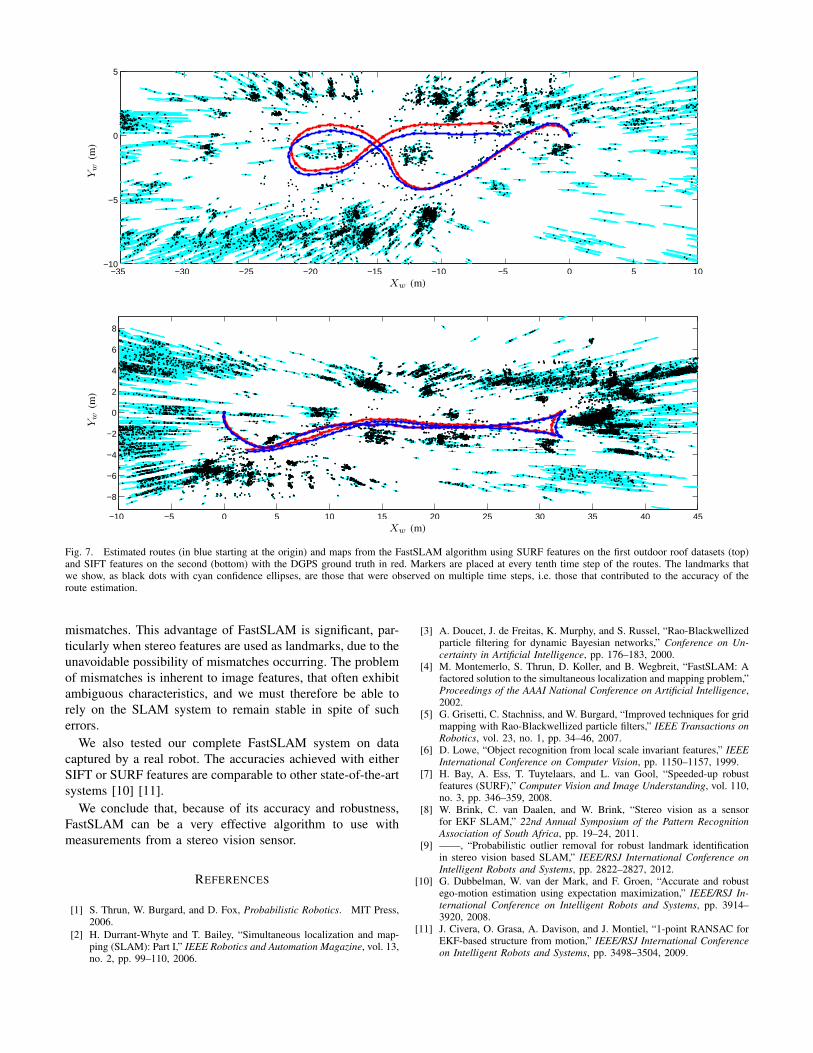
We show the results obtained from two experiments. Thefirst was done using SURF features on the first dataset, andthe second using SIFT features on the second dataset. Theseresults are depicted in Figure 7 with corresponding locationerrors in Figure 6. We see that the Euclidean error from thefirst experiment grows over time. Drift is something that willbe present with any localization system that does not employabsolute measurements (like GPS). In our work we attempt tolimit this drift as much as possible.

We see that both SIFT and SURF can be used to obtainaccurate results. Although we have no way of measuringthe accuracies of the estimated maps, we can observe somestructure and large quantities of landmarks located on theobstacles around which the robot moved.

VII. CONCLUSIONS

In this paper we investigated the use of the FastSLAM algo-rithm with landmarks originating from stereo image features.We explained how image features can be used as landmarks,with associated uncertainties in the form of Gaussian distribu-tions. A measurement function converts features relative to therobot to landmarks in world coordinates and these landmarksare then matched over time, and outliers are identified andrejected. The FastSLAM algorithm then uses a particle filterto maintain the robot states, and for each particle a set ofseparate EKFs to estimate landmark locations.

We tested the system in a controlled simulation environ-ment, and found that FastSLAM can be as accurate as EKFSLAM (when landmark matches are uncontaminated) buthas the advantage of being largely unaffected by landmark

0 20 40 60 80 100 1200

0.5

1

1.5

0 20 40 60 80 100 120 140 160 180 2000

0.5

1

1.5

time (s)

erro

r(m

)

time (s)

erro

r(m

)

Fig. 6. The Euclidean error over time, as measured against DGPS, of theFastSLAM system using SURF features on the first dataset (top) and SIFTfeatures on the second dataset (bottom).

−35 −30 −25 −20 −15 −10 −5 0 5 10−10

−5

0

5

−10 −5 0 5 10 15 20 25 30 35 40 45

−8

−6

−4

−2

0

2

4

6

8

Xw (m)

Yw

(m)

Xw (m)

Yw

(m)

Fig. 7. Estimated routes (in blue starting at the origin) and maps from the FastSLAM algorithm using SURF features on the first outdoor roof datasets (top)and SIFT features on the second (bottom) with the DGPS ground truth in red. Markers are placed at every tenth time step of the routes. The landmarks thatwe show, as black dots with cyan confidence ellipses, are those that were observed on multiple time steps, i.e. those that contributed to the accuracy of theroute estimation.

mismatches. This advantage of FastSLAM is significant, par-ticularly when stereo features are used as landmarks, due to theunavoidable possibility of mismatches occurring. The problemof mismatches is inherent to image features, that often exhibitambiguous characteristics, and we must therefore be able torely on the SLAM system to remain stable in spite of sucherrors.

We also tested our complete FastSLAM system on datacaptured by a real robot. The accuracies achieved with eitherSIFT or SURF features are comparable to other state-of-the-artsystems [10] [11].

We conclude that, because of its accuracy and robustness,FastSLAM can be a very effective algorithm to use withmeasurements from a stereo vision sensor.

REFERENCES

[1] S. Thrun, W. Burgard, and D. Fox, Probabilistic Robotics. MIT Press,2006.

[2] H. Durrant-Whyte and T. Bailey, “Simultaneous localization and map-ping (SLAM): Part I,” IEEE Robotics and Automation Magazine, vol. 13,no. 2, pp. 99–110, 2006.

[3] A. Doucet, J. de Freitas, K. Murphy, and S. Russel, “Rao-Blackwellizedparticle filtering for dynamic Bayesian networks,” Conference on Un-certainty in Artificial Intelligence, pp. 176–183, 2000.

[4] M. Montemerlo, S. Thrun, D. Koller, and B. Wegbreit, “FastSLAM: Afactored solution to the simultaneous localization and mapping problem,”Proceedings of the AAAI National Conference on Artificial Intelligence,2002.

[5] G. Grisetti, C. Stachniss, and W. Burgard, “Improved techniques for gridmapping with Rao-Blackwellized particle filters,” IEEE Transactions onRobotics, vol. 23, no. 1, pp. 34–46, 2007.

[6] D. Lowe, “Object recognition from local scale invariant features,” IEEEInternational Conference on Computer Vision, pp. 1150–1157, 1999.

[7] H. Bay, A. Ess, T. Tuytelaars, and L. van Gool, “Speeded-up robustfeatures (SURF),” Computer Vision and Image Understanding, vol. 110,no. 3, pp. 346–359, 2008.

[8] W. Brink, C. van Daalen, and W. Brink, “Stereo vision as a sensorfor EKF SLAM,” 22nd Annual Symposium of the Pattern RecognitionAssociation of South Africa, pp. 19–24, 2011.

[9] ——, “Probabilistic outlier removal for robust landmark identificationin stereo vision based SLAM,” IEEE/RSJ International Conference onIntelligent Robots and Systems, pp. 2822–2827, 2012.

[10] G. Dubbelman, W. van der Mark, and F. Groen, “Accurate and robustego-motion estimation using expectation maximization,” IEEE/RSJ In-ternational Conference on Intelligent Robots and Systems, pp. 3914–3920, 2008.

[11] J. Civera, O. Grasa, A. Davison, and J. Montiel, “1-point RANSAC forEKF-based structure from motion,” IEEE/RSJ International Conferenceon Intelligent Robots and Systems, pp. 3498–3504, 2009.