Introduction to Matlab

Ela P ↪ekalska, Marjolein van der Glas

Pattern Recognition Group, Faculty of Applied Sciences

Delft University of Technology

2001 - 2004

Send comments to ela@ph.tn.tudelft.nl

Contents

Introduction 1Preliminaries . . . . . . . . . . . . . . . . . . . . . . . . . . . . . . . . . . . . . . . . . . . . . . 3

1 Getting started with Matlab 41.1 Input via the command-line . . . . . . . . . . . . . . . . . . . . . . . . . . . . . . . . . . . . . . 41.2 help-facilities . . . . . . . . . . . . . . . . . . . . . . . . . . . . . . . . . . . . . . . . . . . . . . 51.3 Interrupting a command or program . . . . . . . . . . . . . . . . . . . . . . . . . . . . . . . . . 61.4 Path . . . . . . . . . . . . . . . . . . . . . . . . . . . . . . . . . . . . . . . . . . . . . . . . . . . 61.5 Workspace issues . . . . . . . . . . . . . . . . . . . . . . . . . . . . . . . . . . . . . . . . . . . . 61.6 Saving and loading data . . . . . . . . . . . . . . . . . . . . . . . . . . . . . . . . . . . . . . . . 7

2 Basic syntax and variables 72.1 Matlab as a calculator . . . . . . . . . . . . . . . . . . . . . . . . . . . . . . . . . . . . . . . . 72.2 An introduction to floating-point numbers . . . . . . . . . . . . . . . . . . . . . . . . . . . . . . 82.3 Assignments and variables . . . . . . . . . . . . . . . . . . . . . . . . . . . . . . . . . . . . . . . 9

3 Mathematics with vectors and matrices 103.1 Vectors . . . . . . . . . . . . . . . . . . . . . . . . . . . . . . . . . . . . . . . . . . . . . . . . . 10

3.1.1 Colon notation and extracting parts of a vector . . . . . . . . . . . . . . . . . . . . . . . 113.1.2 Column vectors and transposing . . . . . . . . . . . . . . . . . . . . . . . . . . . . . . . 123.1.3 Product, divisions and powers of vectors . . . . . . . . . . . . . . . . . . . . . . . . . . . 13

3.2 Matrices . . . . . . . . . . . . . . . . . . . . . . . . . . . . . . . . . . . . . . . . . . . . . . . . . 163.2.1 Special matrices . . . . . . . . . . . . . . . . . . . . . . . . . . . . . . . . . . . . . . . . 163.2.2 Building matrices and extracting parts of matrices . . . . . . . . . . . . . . . . . . . . . 173.2.3 Operations on matrices . . . . . . . . . . . . . . . . . . . . . . . . . . . . . . . . . . . . 20

4 Visualization 224.1 Simple plots . . . . . . . . . . . . . . . . . . . . . . . . . . . . . . . . . . . . . . . . . . . . . . . 224.2 Several functions in one figure . . . . . . . . . . . . . . . . . . . . . . . . . . . . . . . . . . . . . 234.3 Other 2D plotting features - optional . . . . . . . . . . . . . . . . . . . . . . . . . . . . . . . . . 244.4 Printing . . . . . . . . . . . . . . . . . . . . . . . . . . . . . . . . . . . . . . . . . . . . . . . . . 254.5 3D line plots . . . . . . . . . . . . . . . . . . . . . . . . . . . . . . . . . . . . . . . . . . . . . . 264.6 Plotting surfaces . . . . . . . . . . . . . . . . . . . . . . . . . . . . . . . . . . . . . . . . . . . . 264.7 Animations - optional . . . . . . . . . . . . . . . . . . . . . . . . . . . . . . . . . . . . . . . . . 27

5 Control flow 285.1 Logical and relational operators . . . . . . . . . . . . . . . . . . . . . . . . . . . . . . . . . . . . 28

5.1.1 The command find . . . . . . . . . . . . . . . . . . . . . . . . . . . . . . . . . . . . . . 305.2 Conditional code execution . . . . . . . . . . . . . . . . . . . . . . . . . . . . . . . . . . . . . . 315.3 Loops . . . . . . . . . . . . . . . . . . . . . . . . . . . . . . . . . . . . . . . . . . . . . . . . . . 335.4 Evaluation of logical and relational expressions in the control flow structures . . . . . . . . . . 35

6 Numerical analysis 366.1 Curve fitting . . . . . . . . . . . . . . . . . . . . . . . . . . . . . . . . . . . . . . . . . . . . . . 366.2 Interpolation . . . . . . . . . . . . . . . . . . . . . . . . . . . . . . . . . . . . . . . . . . . . . . 376.3 Evaluation of a function . . . . . . . . . . . . . . . . . . . . . . . . . . . . . . . . . . . . . . . . 37

6.3.1 Inline functions . . . . . . . . . . . . . . . . . . . . . . . . . . . . . . . . . . . . . . . . . 386.4 Integration and differentiation . . . . . . . . . . . . . . . . . . . . . . . . . . . . . . . . . . . . . 396.5 Numerical computations and the control flow structures . . . . . . . . . . . . . . . . . . . . . . 40

7 Script and function m-files 407.1 Script m-files . . . . . . . . . . . . . . . . . . . . . . . . . . . . . . . . . . . . . . . . . . . . . . 407.2 Function m-file . . . . . . . . . . . . . . . . . . . . . . . . . . . . . . . . . . . . . . . . . . . . . 41

7.2.1 Special function variables . . . . . . . . . . . . . . . . . . . . . . . . . . . . . . . . . . . 437.2.2 Local and global variables . . . . . . . . . . . . . . . . . . . . . . . . . . . . . . . . . . . 447.2.3 Indirect function evaluation - optional . . . . . . . . . . . . . . . . . . . . . . . . . . . . 44

7.3 Scripts vs. functions . . . . . . . . . . . . . . . . . . . . . . . . . . . . . . . . . . . . . . . . . . 46

8 Text 47

8.1 Character strings . . . . . . . . . . . . . . . . . . . . . . . . . . . . . . . . . . . . . . . . . . . . 478.2 Text input and output . . . . . . . . . . . . . . . . . . . . . . . . . . . . . . . . . . . . . . . . . 49

9 Cell arrays and structures - optional 529.1 Cell arrays . . . . . . . . . . . . . . . . . . . . . . . . . . . . . . . . . . . . . . . . . . . . . . . . 529.2 Structures . . . . . . . . . . . . . . . . . . . . . . . . . . . . . . . . . . . . . . . . . . . . . . . . 53

10 Optimizing the performance of Matlab code 5410.1 Vectorization - speed-up of computations . . . . . . . . . . . . . . . . . . . . . . . . . . . . . . 5410.2 Array preallocation . . . . . . . . . . . . . . . . . . . . . . . . . . . . . . . . . . . . . . . . . . . 5510.3 Matlab’s tricks and tips . . . . . . . . . . . . . . . . . . . . . . . . . . . . . . . . . . . . . . . 56

11 File input/output operations 5911.1 Text files . . . . . . . . . . . . . . . . . . . . . . . . . . . . . . . . . . . . . . . . . . . . . . . . 6011.2 Binary files - optional . . . . . . . . . . . . . . . . . . . . . . . . . . . . . . . . . . . . . . . . . 61

12 Writing and debugging Matlab programs 6212.1 Structural programming . . . . . . . . . . . . . . . . . . . . . . . . . . . . . . . . . . . . . . . . 6212.2 Debugging . . . . . . . . . . . . . . . . . . . . . . . . . . . . . . . . . . . . . . . . . . . . . . . . 6412.3 Recommended programming style . . . . . . . . . . . . . . . . . . . . . . . . . . . . . . . . . . . 64

Introduction

During this course you will learn how to use Matlab, to design, and to perform mathematical computations.You will also get acquainted with basic programming. If you learn to use this program well, you will find itvery useful in future, since many technical or mathematical problems can be solved using Matlab.

This text includes all material (with some additional information) that you need to know, however, manythings are treated briefly. Therefore, ”The Student Edition of Matlab” user’s guide should be used as a

complementary book during the course. A sign of a book accompanied by page numbers, placed in theleft margin, indicates where you can find more information. Read the suggested pages to better understandthe concepts discussed. Where no reference to the book appears, it means that only this text explains someideas, since they might be more about general programming than about Matlab. Exercises are marked with

, also in the left margin. The end of an exercise is marked with �.

The text of this course includes some optional parts for volunteers or for more advanced students. Such a partis enclosed between two horizontal lines, with the word ’optional’ on the first line. There is also an ’intermezzo’part, which is not essential, but provides some important information. If you already know how to programin a language, like Pascal or C, then you may find it easier or more interesting to do the optional parts aswell. However, if you do not have any idea about programming, please feel free to skip those fragments. It isimportant that you spend enough time to learn the Matlab basics.

Please test after each section whether you have sufficient understanding of the issues discussed. Use the listsprovided below.

Sections 1-2.You should be able to:• recognize built-in variables;

• define variables and perform computations using them;

• perform basic mathematical operations;

• know how to suppress display with ; (semicolon);

• use the format command to adjust the Command window;

• add and remove variables from the workspace; check which variables are currently present in theworkspace;

• use on-line help to get more information on a command and know how to use the lookfor command;

• use the load and save commands to read/save data to a file;

• access files at different directories (manipulate path-changing commands);

Section 3.You should be able to:• create vectors and matrices with direct assignment (using [ ]);

• use linspace to create vectors;

• create random vectors and matrices;

• create matrices via the commands: eye ones, zeros and diag;

• build a larger matrix from smaller ones;

• use colon notation to create vectors and extract ranges of elements from vectors and matrices;

• extract elements from vectors and matrices with subscript notation, e.g. x(5), A(i,j);

• apply transpose operators to vectors and matrices;

• perform legal addition, subtraction, and multiplication operations on vectors and matrices;

• understand the use of dot operators, like .*, ./,... and know why they are different from the regular *,/,... operators;

• delete elements from vectors and matrices;

• compute inner products and the Euclidean length of vectors;

• create and manipulate complex vectors and matrices.

Section 4.You should be able to:• use the plot command to make simple plots;

• know how to use hold on/off

1

• plot several functions in one figure either in one graphical window or by creating a few smaller ones (theuse of subplot);

• add a title, grid and a legend, describe the axes, change the range of axes;

• use logarithmic axes;

• make simple 3D line plots;

• plot surfaces, contours, change colors;

• send figures to the printer or print them to a file;

• optional: make some fancy plots;

• optional: create Matlab animations.

Section 5.You should be able to:• use relational operators: <, <=, >, >=, ==, ~= and logical operators: &, | and ~;

• understand the logical addressing;

• fully understand how to use the command find, both on vectors and matrices;

• use if...end, if...elseif...end and if...elseif...else...end and switch constructs;

• use for-loops and while-loops and know the difference between them;

• understand how logical expressions are evaluated in the control flow structures.

Section 6.You should be able to:• create and manipulate Matlab polynomials;

• fit a polynomial to data;

• interpolate the data;

• evaluate a function;

• create inline functions;

• integrate and differentiate a function;

• optional: understand how to make approximations of Taylor expansions with the given precision.

Section 7.You should be able to:• edit and run an m-file (both functions and scripts);

• identify the differences between scripts and functions;

• understand the concept of local and global variables;

• create a function with one or more input arguments and one or more output arguments;

• use comment statements to document scripts and functions;

• optional: use the feval command - know how to pass a function name as an input argument to anotherfunction.

Sections 8-9.You should be able to:• create and manipulate string variables, e.g. compare two strings, concatenate them, find a substring in

a string, convert a number/string into a string/number etc;

• use freely and with understanding the text input/output commands: input, disp and fprintf;

• optional: operate on cell arrays and structures;

Section 10.You should be able to:• preallocate memory for vectors or matrices and know why and when this is beneficial;

• replace basic loops with vectorized operations;

• use colon notation to perform vectorized operations;

• understand the two ways of addressing matrix elements using a vector as an index: traditional and logicalindexing;

• use array indexing instead of loops to select elements from a matrix;

2

• use logical indexing and logical functions instead of loops to select elements from matrices;

• understand Matlab’s tricks.

Section 11.You should be able to:• perform low level input and output with fopen, fscanf and fclose;

• understand how to operate on text files (input/output operations);

• get more understanding on the use of fprintf while writing to a file;

• optional: understand how to operate on binary files (input/output operations);

Section 12.You should be able to:• know and understand the importance of structural programming and debugging;

• know how to debug your program;

• have an idea how to write programs using the recommended programming style.

Preliminaries

Below you find a few basic definitions on computers and programming. Please get acquainted with them sincethey introduce key concepts needed in the coming sections:

• A bit (short for binary digit) is the smallest unit of information on a computer. A single bit can holdonly one of two values: 0 or 1. More meaningful information is obtained by combining consecutive bitsinto larger units, such as byte.

• A byte - a unit of 8 bits, being capable of holding a single character. Large amounts of memory areindicated in terms of kilobytes (1024 bytes), megabytes (1024 kilobytes), and gigabytes (1024 megabytes).

• Binary system - a number system that has two unique digits: 0 and 1. Computers are based on sucha system, because of its electrical nature (charged versus uncharged). Each digit position represents adifferent power of 2. The powers of 2 increase while moving from the right most to the left most position,starting from 20 = 1. Here is an example of a binary number and its representation in the decimalsystem:

10110 = 1 ∗ 24 + 0 ∗ 23 + 1 ∗ 22 + 1 ∗ 21 + 0 ∗ 20 = 16 + 0 + 4 + 2 + 0 = 24

• Data is information represented with symbols, e.g. numbers, words, signals or images.

• A command is a instruction to do a specific task.

• An algorithm is a sequence of instructions for the solution of a specific task in a finite number of steps.

• A program is the implementation of an algorithm suitable for execution by a computer.

• A variable is a container that can hold a value. For example, in the expression: x+y, x and y are variables.They can represent numeric values, like 25.5, characters, like ’c’ or character strings, like ’Matlab’.Variables make programs more flexible. When a program is executed, the variables are then replacedwith real data. That is why the same program can process different sets of data.

Every variable has a name (called the variable name) and a data type. A variable’s data type indicatesthe sort of value that the variable represents (see below).

• A constant is a value that never changes. That makes it the opposite of a variable. It can be a numericvalue, a character or a string.

• A data type is a classification of a particular type of information. The most basic data types are:

• integer: a whole number; a number that has no fractional part, e.g. 3.• floating-point: a number with a decimal point, e.g. 3.5 or 1.2e-16 (this stands for 1.2 ∗ 10−16).• character: readable text character, e.g. ’p’.

• A bug is an error in a program, causing the program to stop running, not to run at all or to providewrong results. Some bugs can be very subtle and hard to find. The process of finding and removing bugsis called debugging.

• A file is a collection of data or information that has a name, stored in a computer. There are manydifferent types of files: data files, program files, text files etc.

• An ASCII file is a standardized, readable and editable plain text file.

• A binary file is a file stored in a format, which is computer-readable but not human-readable. Mostnumeric data and all executable programs are stored in binary files. Matlab binary files are those withthe extension ’*.mat’.

3

1 Getting started with Matlab

Matlab is a tool for mathematical (technical) calculations. First, it can be used as a scientific calculator.Next, it allows you to plot or visualize data in many different ways, perform matrix algebra, work withpolynomials or integrate functions. Like in a programmable calculator, you can create, execute and save asequence of commands in order to make your computational process automatic. It can be used to store orretrieve data. In the end, Matlab can also be treated as a user-friendly programming language, which givesthe possibility to handle mathematical calculations in an easy way. In summary, as a computing/programmingenvironment, Matlab is especially designed to work with data sets as a whole such as vectors, matrices andimages. Therefore, PRTOOLS, a toolbox for Pattern Recognition purposes, and DIPLIB, a toolbox forImage Processing, have been developed under Matlab.

Under Windows, you can start Matlab by double clicking on the Matlab icon that should be on the desktopof your computer; on unix systems, type matlab at the command line. Running Matlab creates one or morewindows on your screen. The most important is the Command Window , which is the place you interact withMatlab, i.e. it is used to enter commands and display text results. The string >> is the Matlab prompt (orEDU>> for the Student Edition). When the Command Window is active, a cursor appears after the prompt,indicating that Matlab is waiting for your command. Matlab responds by printing text in the CommandWindow or by creating a Figure Window for graphics. To exit Matlab use the command exit or quit.

1.1 Input via the command-line

2-10 Matlab is an interactive system; commands followed by Enter are executed immediately. The results are,if desired, displayed on screen. However, execution of a command will be possible if the command is typedaccording to the rules. Table 1 shows a list of commands used to solve indicated mathematical equations (a,b, x and y are numbers). Below you find basic information to help you starting with Matlab :

• Commands in Matlab are executed by pressing Enter or Return. The output will be displayed onscreen immediately. Try the following:

>> 3 + 7.5

>> 18/4

>> 3 * 7

Note that spaces are not important in Matlab.

• The result of the last performed computation is ascribed to the variable ans, which is an example of aMatlab built-in variable. It can be used in the next command. For instance:

>> 14/4

ans =

3.5000

>> ans^(-6)

ans =

5.4399e-04

5.4399e-04 is a computer notation of 5.4399 ∗ 10−4 (see Preliminaries). Note that ans is alwaysoverwritten by the last command.

• You can also define your own variables. Look how the information is stored in the variables a and b:

>> a = 14/4

a =

3.5000

>> b = a^(-6)

b =

5.4399e-04

Read Preliminaries to better understand the concept of variables. You will learn more on Matlab

variables in section 2.3.

• When the command is followed by a semicolon ’;’, the output is suppressed. Check the difference betweenthe following expressions:

>> 3 + 7.5

>> 3 + 7.5;

4

• It is possible to execute more than one command at the same time; the separate commands should thenbe divided by commas (to display the output) or by semicolons (to suppress the output display), e.g.:

>> sin(pi/4), cos(pi); sin(0)

ans =

0.7071

ans =

0

Note that the value of cos(pi) is not printed.

• By default, Matlab displays only 5 digits. The command format long increases this number to 15,format short reduces it to 5 again. For instance:

>> 312/56

ans =

5.5714

>> format long

>> 312/56

ans =

5.57142857142857

• The output may contain some empty lines; this can be suppressed by the command format compact.In contrast, the command format loose will insert extra empty lines.

256 • To enter a statement that is too long to be typed in one line, use three periods ’...’ followed by Enter

or Return. For instance:

>> sin(1) + sin(2) - sin(3) + sin(4) - sin(5) + sin(6) - ...

sin(8) + sin(9) - sin(10) + sin(11) - sin(12)

ans =

1.0357

• Matlab is case sensitive, for example, a is written as a in Matlab; A will result then in an error.

• All text after a percent sign % until the end of a line is treated as a comment. Enter e.g. the following:

>> sin(3.14159) % this is an approximation of sin(pi)

You will notice that some examples in this text are followed by comments. They are meant for you andyou should skip them while typing those examples.

• Previous commands can be fetched back with the ↑ -key. The command can also be changed, the ←and → -keys may be used to move around in a line and edit it. In case of a long line, Ctrl-a and Ctrl-e

might be useful; they allow to move the cursor at the beginning or the end of the line, respectively.

• To recall the most recent command starting from e.g. c, type c at the prompt followed by the ↑ -key.

Similarly, cos followed by the ↑ -key will find the last command starting from cos.

Since Matlab executes the command immediately, it might be useful to have an idea of the expected outcome.You might be surprised how long it takes to print out a 1000× 1000 matrix!

1.2 help-facilities

Matlab provides assistance through extensive online help. The help command is the simplest way to get349-359 help. It displays the list of all possible topics. To get a more general introduction to help, try:

>> help help

If you already know the topic or command, you can ask for a more specified help. For instance:

>> help ops

gives information on the operators and special characters in Matlab. The topic you want help on must beexact and spelled correctly. The lookfor command is more useful if you do not know the exact name of thecommand or topic. For example:

5

Mathematical notation Matlab command

a + b a + b

a− b a - b

ab a * bab a / b or b \ a

xb x^b√x sqrt(x) or x^0.5

|x| abs(x)

π pi

4 · 103 4e3 or 4*10^3

i i or j

3− 4i 3-4*i or 3-4*j

e, ex exp(1), exp(x)ln x, log x log(x), log10(x)sin x, arctanx, ... sin(x), atan(x),...

Table 1: Translation of mathematical notation to Matlab commands.

>> lookfor inverse

displays a list of commands, with a short description, for which the word inverse is included in its help-text.You can also use an incomplete name, e.g. lookfor inv. Besides the help and lookfor commands, thereis also a separate mouse driven help. The helpwin command opens a new window on screen which can be

353-354 browsed in an interactive way.

Exercise 1.

• Is the inverse cosine function, known as cos−1 or arccos, one of the Matlab’s elementary functions?

• Does Matlab have a mathematical function to calculate the greatest common divisor?

• Look for information on logarithms.

Use help or lookfor to find out. �

1.3 Interrupting a command or program

Sometimes you might spot an error in your command or program. Due to this error it can happen thatthe command or program does not stop. Pressing Ctrl-C (or Ctrl-Break on PC) forces Matlab to stopthe process. Sometimes, however, you may need to press a few times. After this the Matlab prompt (>>)re-appears. This may take a while, though.

1.4 Path

In Matlab, commands or programs are contained in m-files, which are just plain text files and have an37-39 extension ’.m’. The m-file must be located in one of the directories which Matlab automatically searches.

The list of these directories can be listed by the command path. One of the directories that is always taken intoaccount is the current working directory, which can be identified by the command pwd. Use path, addpath andrmpath functions to modify the path. It is also possible to access the path browser from the File menu-bar,instead.

Exercise 2.Type path to check which directories are placed on your path. Add you personal directory to the path(assuming that you created your personal directory for working with Matlab). �

1.5 Workspace issues

If you work in the Command Window, Matlab memorizes all commands that you entered and all variablesthat you created. These commands and variables are said to reside in the Matlab workspace. They might be

624,25

easily recalled when needed, e.g. to recall previous commands, the ↑ -key is used. Variables can be verified

with the commands who, which gives a list of variables present in the workspace, and whos, which includesalso information on name, number of allocated bytes and class of variables. For example, assuming that youperformed all commands from section 1.1, after typing who you should get the following information:

6

>> who

Your variables are:

a ans b x

The command clear <name> deletes the variable <name> from the Matlab workspace, clear or clear all

removes all variables. This is useful when starting a new exercise. For example:

>> clear a x

>> who

Your variables are:

ans b

1.6 Saving and loading data

The easiest way to save or load Matlab variables is by using (clicking) the File menu-bar, and then selecting26 the Save Workspace as... or Load Workspace... items respectively. Also Matlab commands exist which

save data to files and which load data from files.

The command save allows for saving your workspace variables either into a binary file or an ASCII file (checkPreliminaries on binary and ASCII files). Binary files automatically get the ’.mat’ extension, which is nottrue for ASCII files. However, it is recommended to add a ’.txt’ or .dat extension.

Exercise 3.Learn how to use the save command by exercising:

>> s1 = sin(pi/4);

>> c1 = cos(pi/4); c2 = cos(pi/2);

>> str = ’hello world’; % this is a string

>> save % saves all variables in binary format to matlab.mat

>> save data % saves all variables in binary format to data.mat

>> save numdata s1, c1 % saves numeric variables s1 and c1 to numdata.mat

>> save strdata str % saves a string variable str to strdata.mat

>> save allcos.dat c* -ascii % saves c1,c2 in 8-digit ascii format to allcos.dat

�

The load command allows for loading variables into the workspace. It uses the same syntax as save.

Exercise 4.Assuming that you have done the previous exercise, try to load variables from the created files. Before eachload command, clear the workspace and after loading check which variables are present in the workspace (usewho).

>> load % loads all variables from the file matlab.mat

>> load data s1 c1 % loads only specified variables from the file data.mat

>> load str data % loads all variables from the file strdata.mat

It is also possible to read ASCII files that contain rows of space separated values. Such a file may containcomments that begin with a percent character. The resulting data is placed into a variable with the samename as the ASCII file (without the extension). Check, for example:

>> load allcos.dat % loads data from allcos.dat into variable allcos

>> who % lists variables present in the workspace now

�

2 Basic syntax and variables

2.1 Matlab as a calculator

There are three kinds of numbers used in Matlab: integers, real numbers and complex numbers. In addition,4-7

14-1727

Matlab has representations of the non-numbers: Inf, for positive infinity, generated e.g. by 1/0, and NaN,Not-a-Number, obtained as a result of the mathematically undefined operations such as 0/0 or ∞ - ∞.

7

You have already got some experience with Matlab and you know that it can be used as a calculator. To dothat you can, for example, simply type:

>> (23*17)/7

The result will be:

ans =

55.8571

Matlab has six basic arithmetic operations, such as: +, -, *, / or \ (right and left divisions) and ^ (power).Note that the two division operators are different:

>> 19/3 % mathematically: 19/3

ans =

6.3333

>> 19\3, 3/19 % mathematically: 3/19

ans =

0.1579

ans =

0.1579

Basic built-in functions, trigonometric, exponential, etc, are available for a user. Try help elfun to get thelist of elementary functions.

Exercise 5.Evaluate the following expressions by hand and use Matlab to check the answers. Note the difference betweenthe left and right divisors. Use help to learn more on commands rounding numbers, such as: round, floor,ceil, etc.

• 2/2 ∗ 3• 8 ∗ 5\4• 8 ∗ (5\4)• 7− 5 ∗ 4\9• 6− 2/5+ 7^2− 1

• 10/2\5− 3 + 2 ∗ 4

• 3^2/4

• 3^2^3

• 2 + round (6/9+ 3 ∗ 2)/2• 2 + floor (6/9+ 3 ∗ 2)/2• 2 + ceil (6/9 + 3 ∗ 2)/2• x = pi/3, x = x− 1, x = x + 5, x = abs(x)/x

�

Exercise 6.Define the format in Matlab such that empty lines are suppressed and the output is given with 15 digits.Calculate:

>> pi

>> sin(pi)

Note that the answer is not exactly 0. Use the command format to put Matlab in its standard-format. �

intermezzo

2.2 An introduction to floating-point numbers

In a computer, numbers can be represented only in a discrete form. It means that numbers are stored within286 a limited range and with a finite precision. Integers can be represented exactly with the base of 2 (read

Preliminaries on bits and the binary system). The typical size of an integer is 16 bits, so the largestpositive integer, which can be stored, is 216 = 65536. If negative integers are permitted, then 16 bits allow forrepresenting integers between −32768 and 32767. Within this range, operations defined on the set of integerscan be performed exactly.

However, this is not valid for other real numbers. In practice, computers are integer machines and are capableof representing real numbers only by using complicated codes. The most popular code is the floating point

standard. The term floating point is derived from the fact that there is no fixed number of digits before andafter the decimal point, meaning that the decimal point can float. Note that most floating-point numbers thata computer can represent are just approximations. Therefore, care should be taken that these approximationslead to reasonable results. If a programmer is not careful, small discrepancies in the approximations can causemeaningless results. Note the difference between e.g. the integer arithmetic and floating-point arithmetic:

8

Integer arithmetic: Floating-point arithmetic2 + 4 = 6 18/7 = 2.5714

3 * 4 = 12 2.5714 * 7 = 17.9998

25/11 = 2 10000/3 = 3.3333e+03

When describing floating-point numbers, precision refers to the number of bits used for the fractional part.The larger the precision, the more exact fractional quantities can be represented. Floating-point numbers areoften classified as single precision or double precision. A double-precision number uses twice as many bits asa single-precision value, so it can represent fractional values much better. However, the precision itself is notdouble. The extra bits are also used to increase the range of magnitudes that can be represented.

Matlab relies on a computer’s floating point arithmetic. You could have noticed that in the last exercise408-410 since the value of sin(π) was almost zero, and not completely zero. It came from the fact that both the value

of π is represented with a finite precision and the sin function is also approximated.

The fundamental type in Matlab is double, which stands for a representation with a double precision. It uses64 bits. The single precision obtained by using the single type offers 32 bits. Since most numeric operationsrequire high accuracy the double type is used by default. This means, that when the user is inputting integervalues in Matlab (for instance, k = 4), the data is still stored in double format.

The relative accuracy might be defined as the smallest positive number ε that added to 1, creates the resultlarger than 1, i.e. 1 + ε > 1. It means that in floating-point arithmetic, for positive values smaller than ε, theresult equals to 1 (in exact arithmetic, of course, the result is always larger than 1). In Matlab, ε is storedin the built-in variable eps ≈ 2.2204e-16. This means that the relative accuracy of individual arithmeticoperations is about 15 digits.

end intermezzo

2.3 Assignments and variables

Working with complex numbers is easily done with Matlab.

Exercise 7.Choose two complex numbers, for example -3 + 2i and 5 - 7i. Add, subtract, multiply, and divide thesetwo numbers. �

During this exercise, the complex numbers had to be typed four times. To reduce this, assign each number to4-6

10-12a variable. For the previous exercise, this results in:

>> z = -3 + 2*i; w = 5 - 7*i;

>> y1 = z + w; y2 = z - w;

>> y3 = z * w;

>> y4 = z / w; y5 = w \ z;

Formally, there is no need to declare (i.e. define the name, size and the type of) a new variable in Matlab. Avariable is simply created by an assignment (e.g. z = -3 + 2*i), i.e. values are assigned to variables. Eachnewly created numerical variable is always of the double type, i.e. real numbers are approximated with thehighest possible precision. You can change this type by converting it into e.g. the single type1. In some cases,when huge matrices should be handled and precision is not very important, this might be a way to proceed.Also, when only integers are taken into consideration, it might be useful to convert the double representationsinto e.g. int321 integer type. Note that integer numbers are represented exactly, no matter which numerictype is used, as long as the number can be represented in the number of bits used in the numeric type.

Bear in mind that undefined values cannot be assigned to variables. So, the following is not possible:

>> clear x; % to make sure that x does not exist

>> f = x^2 + 4 * sin(x)

It becomes possible by:

>> x = pi / 3; f = x^2 + 4 * sin(x)

Variable name begins with a letter, followed by letters, numbers or underscores. Matlab recognizes only first31 characters of the name.

Exercise 8.Here are some examples of different types of Matlab variables. You do not need to understand them all now,since you will learn more about them during the course. Create them manually in Matlab:

1a variable a is converted into a different type by performing e.g. a = single(a), a = int32(a) etc.

9

Variable name Value/meaning

ans the default variable name used for storing the last resultpi π = 3.14159...eps the smallest positive number that added to 1, creates a result larger than 1inf representation for positive infinity, e.g. 1/0nan or NaN representation for not-a-number, e.g. 0/0

i or j i = j =√−1

nargin/nargout number of function input/output arguments usedrealmin/realmax the smallest/largest usable positive real number

Table 2: Built-in variables in Matlab.

>> this_is_my_very_simple_variable_today = 5 % check what happens; the name is very long

>> 2t = 8 % what is the problem with this command?

>> M = [1 2; 3 4; 5 6] % a matrix

>> c = ’E’ % a character

>> str = ’Hello world’ % a string

>> m = [’J’,’o’,’h’,’n’] % try to guess what it is

Check the types by using the command whos. Use clear <name> to remove a variable from the workspace. �

As you already know, Matlab variables can be created by an assignment. There is also a number of built-invariables, e.g. pi, eps or i, summarized in Table 2. In addition to creating variables by assigning values to

7,45,84 them, another possibility is to copy one variable, e.g. b into another, e.g. a. In this way, the variable a isautomatically created (if a already existed, its previous value is lost):

>> b = 10.5;

>> a = b;

A variable can be also created as a result of the evaluated expression:

>> a = 10.5; c = a^2 + sin(pi*a)/4;

or by loading data from text or ’*.mat’ files.

If min is the name of a function (see help min), then a defined, e.g. as:

>> b = 5; c = 7;

>> a = min (b,c); % create a as the minimum of b and c

will call that function, with the values b and c as parameters. The result of this function (its return value) willbe written (assigned) into a. So, variables can be created as results of the execution of built-in or user-definedfunctions (you will learn more how to built own functions in section 7.2).

Important: do not use variable names which are defined as function names (for instance mean or error)2! Ifyou are going to use a suspicious variable name, use help <name> to find out if the function already exists.

3 Mathematics with vectors and matrices

The basic element of Matlab is a matrix (or an array). Special cases are:

• a 1× 1-matrix: a scalar or a single number;

• a matrix existing only of one row or one column: a vector.

Note that Matlab may behave differently depending on the input, whether it is a number, a vector or a 2Dmatrix.

3.1 Vectors

Row vectors are lists of numbers separated either by commas or by spaces. They are examples of simple arrays .41-49 First element has index 1. The number of entries is known as the length of the vector (the command length

exists as well). Their entities are referred to as elements or components. The entries must be enclosed in [ ]:2There is always one exception of the rule: variable i is often used as counter in a loop, while it is also used as i =

√

−1.

10

>> v = [-1 sin(3) 7]

v =

-1.0000 0.1411 7.0000

>> length(v)

ans =

3

A number of operations can be done on vectors. A vector can be multiplied by a scalar, or added/subtractedto/from another vector with the same length, or a number can be added/subtracted to/from a vector. Allthese operations are carried out element-by-element. Vectors can be also built from the already existing ones.

>> v = [-1 2 7]; w = [2 3 4];

>> z = v + w % an element-by-element sum

z =

1 5 11

>> vv = v + 2 % add 2 to all elements of vector v

vv =

1 4 9

>> t = [2*v, -w]

ans =

-2 4 14 -2 -3 -4

Also, a particular value can be changed or displayed:

>> v(2) = -1 % change the 2nd element of v

v =

-1 -1 7

>> w(2) % display the 2nd element of w

ans =

3

3.1.1 Colon notation and extracting parts of a vector

A colon notation is an important shortcut, used when producing row vectors (see Table 3 and help colon):

>> 2:5

ans =

2 3 4 5

>> -2:3

ans =

-2 -1 0 1 2 3

In general, first:step:last produces a vector of entities with the value first, incrementing by the step

until it reaches last:

>> 0.2:0.5:2.4

ans =

0.2000 0.7000 1.2000 1.7000 2.2000

>> -3:3:10

ans =

-3 0 3 6 9

>> 1.5:-0.5:-0.5 % negative step is also possible

ans =

1.5000 1.0000 0.5000 0 -0.5000

Parts of vectors can be extracted by using a colon notation:

>> r = [-1:2:6, 2, 3, -2] % -1:2:6 => -1 1 3 5

r =

-1 1 3 5 2 3 -2

11

>> r(3:6) % get elements of r which are on the positions from 3 to 6

ans =

3 5 2 3

>> r(1:2:5) % get elements of r which are on the positions 1, 3 and 5

ans =

-1 3 2

>> r(5:-1:2) % what will you get here?

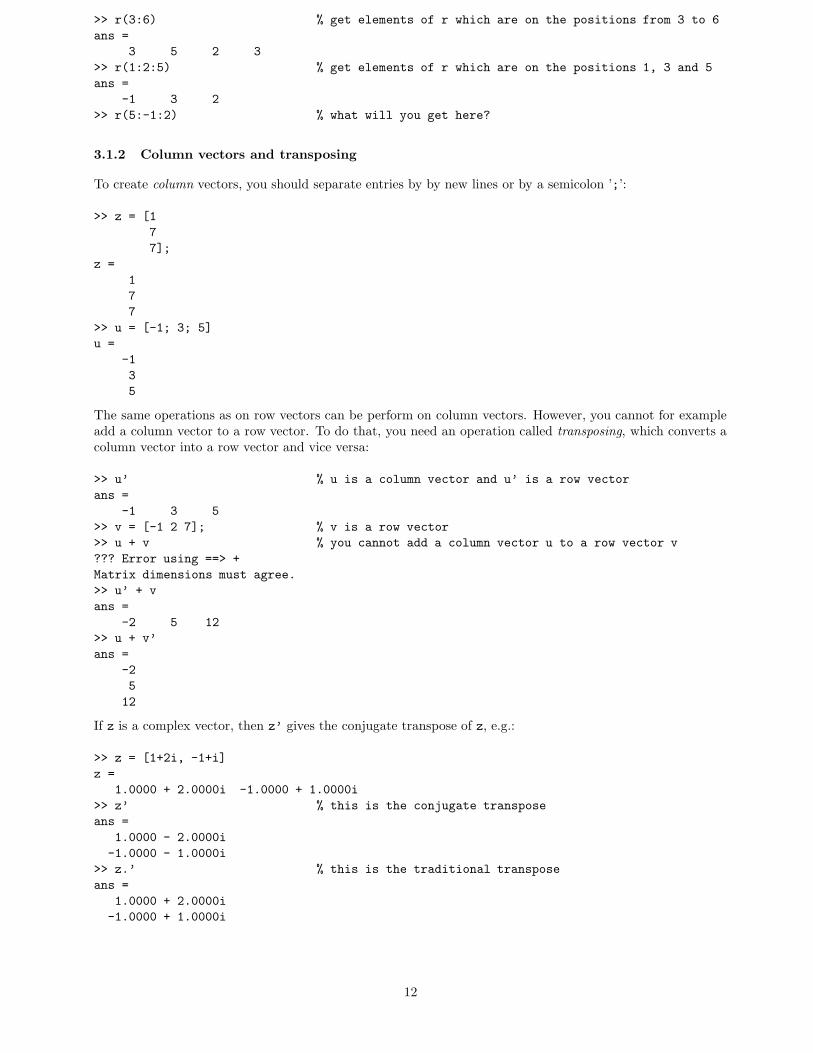
3.1.2 Column vectors and transposing

To create column vectors, you should separate entries by by new lines or by a semicolon ’;’:

>> z = [1

7

7];

z =

1

7

7

>> u = [-1; 3; 5]

u =

-1

3

5

The same operations as on row vectors can be perform on column vectors. However, you cannot for exampleadd a column vector to a row vector. To do that, you need an operation called transposing, which converts acolumn vector into a row vector and vice versa:

>> u’ % u is a column vector and u’ is a row vector

ans =

-1 3 5

>> v = [-1 2 7]; % v is a row vector

>> u + v % you cannot add a column vector u to a row vector v

??? Error using ==> +

Matrix dimensions must agree.

>> u’ + v

ans =

-2 5 12

>> u + v’

ans =

-2

5

12

If z is a complex vector, then z’ gives the conjugate transpose of z, e.g.:

>> z = [1+2i, -1+i]

z =

1.0000 + 2.0000i -1.0000 + 1.0000i

>> z’ % this is the conjugate transpose

ans =

1.0000 - 2.0000i

-1.0000 - 1.0000i

>> z.’ % this is the traditional transpose

ans =

1.0000 + 2.0000i

-1.0000 + 1.0000i

12

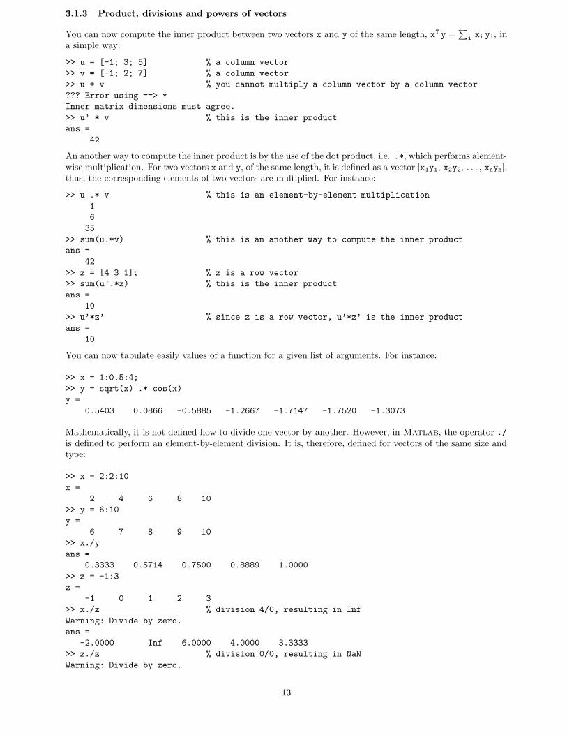
3.1.3 Product, divisions and powers of vectors

You can now compute the inner product between two vectors x and y of the same length, xT y =∑

i xi yi, ina simple way:

>> u = [-1; 3; 5] % a column vector

>> v = [-1; 2; 7] % a column vector

>> u * v % you cannot multiply a column vector by a column vector

??? Error using ==> *

Inner matrix dimensions must agree.

>> u’ * v % this is the inner product

ans =

42

An another way to compute the inner product is by the use of the dot product, i.e. .*, which performs alement-wise multiplication. For two vectors x and y, of the same length, it is defined as a vector [x1y1, x2y2, . . . , xnyn],thus, the corresponding elements of two vectors are multiplied. For instance:

>> u .* v % this is an element-by-element multiplication

1

6

35

>> sum(u.*v) % this is an another way to compute the inner product

ans =

42

>> z = [4 3 1]; % z is a row vector

>> sum(u’.*z) % this is the inner product

ans =

10

>> u’*z’ % since z is a row vector, u’*z’ is the inner product

ans =

10

You can now tabulate easily values of a function for a given list of arguments. For instance:

>> x = 1:0.5:4;

>> y = sqrt(x) .* cos(x)

y =

0.5403 0.0866 -0.5885 -1.2667 -1.7147 -1.7520 -1.3073

Mathematically, it is not defined how to divide one vector by another. However, in Matlab, the operator ./is defined to perform an element-by-element division. It is, therefore, defined for vectors of the same size andtype:

>> x = 2:2:10

x =

2 4 6 8 10

>> y = 6:10

y =

6 7 8 9 10

>> x./y

ans =

0.3333 0.5714 0.7500 0.8889 1.0000

>> z = -1:3

z =

-1 0 1 2 3

>> x./z % division 4/0, resulting in Inf

Warning: Divide by zero.

ans =

-2.0000 Inf 6.0000 4.0000 3.3333

>> z./z % division 0/0, resulting in NaN

Warning: Divide by zero.

13

ans =

1 NaN 1 1 1

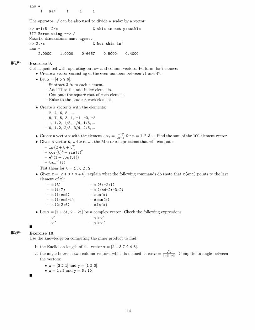
The operator ./ can be also used to divide a scalar by a vector:

>> x=1:5; 2/x % this is not possible

??? Error using ==> /

Matrix dimensions must agree.

>> 2./x % but this is!

ans =

2.0000 1.0000 0.6667 0.5000 0.4000

Exercise 9.Get acquainted with operating on row and column vectors. Perform, for instance:• Create a vector consisting of the even numbers between 21 and 47.

• Let x = [4 5 9 6].

– Subtract 3 from each element.– Add 11 to the odd-index elements.– Compute the square root of each element.– Raise to the power 3 each element.

• Create a vector x with the elements:

– 2, 4, 6, 8, ...– 9, 7, 5, 3, 1, -1, -3, -5

– 1, 1/2, 1/3, 1/4, 1/5, ...– 0, 1/2, 2/3, 3/4, 4/5, ...

• Create a vector x with the elements: xn = (−1)n

2n−1for n = 1, 2, 3, ... Find the sum of the 100-element vector.

• Given a vector t, write down the Matlab expressions that will compute:

– ln (2 + t + t2)– cos (t)2 − sin (t)2

– et (1 + cos (3t))– tan−1(t)

Test them for t = 1 : 0.2 : 2.

• Given x = [2 1 3 7 9 4 6], explain what the following commands do (note that x(end) points to the lastelement of x):

– x (3)

– x (1:7)

– x (1:end)

– x (1:end-1)

– x (2:2:6)

– x (6:-2:1)

– x (end-2:-3:2)

– sum(x)

– mean(x)

– min(x)

• Let x = [1 + 3i, 2− 2i] be a complex vector. Check the following expressions:

– x′

– x.′– x ∗ x′– x ∗ x.′

�

Exercise 10.Use the knowledge on computing the inner product to find:

1. the Euclidean length of the vector x = [2 1 3 7 9 4 6].

2. the angle between two column vectors, which is defined as cosα = xTy

||x|| ||y|| . Compute an angle between

the vectors:

• x = [3 2 1] and y = [1 2 3]• x = 1 : 5 and y = 6 : 10

�

14

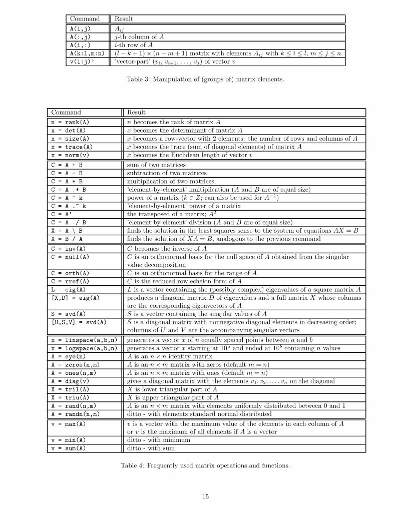
Command Result

A(i,j) Aij

A(:,j) j-th column of AA(i,:) i-th row of AA(k:l,m:n) (l − k + 1)× (n−m + 1) matrix with elements Aij with k ≤ i ≤ l, m ≤ j ≤ nv(i:j)’ ’vector-part’ (vi, vi+1, . . . , vj) of vector v

Table 3: Manipulation of (groups of) matrix elements.

Command Result

n = rank(A) n becomes the rank of matrix Ax = det(A) x becomes the determinant of matrix Ax = size(A) x becomes a row-vector with 2 elements: the number of rows and columns of Ax = trace(A) x becomes the trace (sum of diagonal elements) of matrix Ax = norm(v) x becomes the Euclidean length of vector v

C = A + B sum of two matricesC = A - B subtraction of two matricesC = A * B multiplication of two matricesC = A .* B ’element-by-element’ multiplication (A and B are of equal size)C = A ^ k power of a matrix (k ∈ Z; can also be used for A−1)C = A .^ k ’element-by-element’ power of a matrixC = A’ the transposed of a matrix; AT

C = A ./ B ’element-by-element’ division (A and B are of equal size)X = A \ B finds the solution in the least squares sense to the system of equations AX = BX = B / A finds the solution of XA = B, analogous to the previous command

C = inv(A) C becomes the inverse of AC = null(A) C is an orthonormal basis for the null space of A obtained from the singular

value decompositionC = orth(A) C is an orthonormal basis for the range of AC = rref(A) C is the reduced row echelon form of AL = eig(A) L is a vector containing the (possibly complex) eigenvalues of a square matrix A[X,D] = eig(A) produces a diagonal matrix D of eigenvalues and a full matrix X whose columns

are the corresponding eigenvectors of AS = svd(A) S is a vector containing the singular values of A[U,S,V] = svd(A) S is a diagonal matrix with nonnegative diagonal elements in decreasing order;

columns of U and V are the accompanying singular vectors

x = linspace(a,b,n) generates a vector x of n equally spaced points between a and bx = logspace(a,b,n) generates a vector x starting at 10a and ended at 10b containing n valuesA = eye(n) A is an n× n identity matrixA = zeros(n,m) A is an n×m matrix with zeros (default m = n)A = ones(n,m) A is an n×m matrix with ones (default m = n)A = diag(v) gives a diagonal matrix with the elements v1, v2, . . . , vn on the diagonalX = tril(A) X is lower triangular part of AX = triu(A) X is upper triangular part of AA = rand(n,m) A is an n×m matrix with elements uniformly distributed between 0 and 1A = randn(n,m) ditto - with elements standard normal distributed

v = max(A) v is a vector with the maximum value of the elements in each column of Aor v is the maximum of all elements if A is a vector

v = min(A) ditto - with minimumv = sum(A) ditto - with sum

Table 4: Frequently used matrix operations and functions.

15

3.2 Matrices

Row and column vectors are special types of matrices. An n × k matrix is a rectangular array of numbershaving n rows and k columns. Defining a matrix in Matlab is similar to defining a vector. The generalization

49-6175-86

is straightforward, if you see that a matrix consists of row vectors (or column vectors). Commas or spaces areused to separate elements in a row, and semicolons are used to separate individual rows. For example, the

matrix A =

1 2 3

4 5 6

7 8 9

is defined as:

>> A = [1 2 3; 4 5 6; 7 8 9] % row by row input

A =

1 2 3

4 5 6

7 8 9

Another examples are, for instance:

>> A2 = [1:4; -1:2:5]

A2 =

1 2 3 4

-1 1 3 5

>> A3 = [1 3

-4 7]

A3 =

1 3

-4 7

From that point of view, a row vector is a 1× k matrix and a column vector is an n× 1 matrix. Transposinga vector changes it from a row to a column or the other way around. This idea can be extended to a matrix,where transposing interchanges rows with the corresponding columns, as in the example:

>> A2

A2 =

1 2 3 4

-1 1 3 5

>> A2’ % transpose of A2

ans =

1 -1

2 1

3 3

4 5

>> size(A2) % returns the size (dimensions) of A2: 2 rows, 4 columns

ans =

2 4

>> size(A2’)

ans =

4 2

3.2.1 Special matrices

There is a number of built-in matrices of size specified by the user (see Table 4). A few examples are givenbelow:

>> E = [] % an empty matrix of 0-by-0 elements!

E =

[]

>> size(E)

ans =

0 0

>> I = eye(3); % the 3-by-3 identity matrix

I =

16

1 0 0

0 1 0

0 0 1

>> x = [2; -1; 7]; I*x % I is such that for any 3-by-1 x holds I*x = x

ans =

2

-1

7

>> r = [1 3 -2]; R = diag(r) % create a diagonal matrix with r on the diagonal

R =

1 0 0

0 3 0

0 0 -2

>> A = [1 2 3; 4 5 6; 7 8 9];

>> diag(A) % extracts the diagonal entries of A

ans =

1

5

9

>> B = ones(3,2)

B =

1 1

1 1

1 1

>> C = zeros (size(C’)) % a matrix of all zeros of the size given by C’

C =

0 0 0

0 0 0

>> D = rand(2,3) % a matrix of random numbers; you will get a different one!

D =

0.0227 0.9101 0.9222

0.0299 0.0640 0.3309

>> v = linspace(1,2,4) % a vector is also an example of a matrix

v =

1.0000 1.3333 1.6667 2.0000

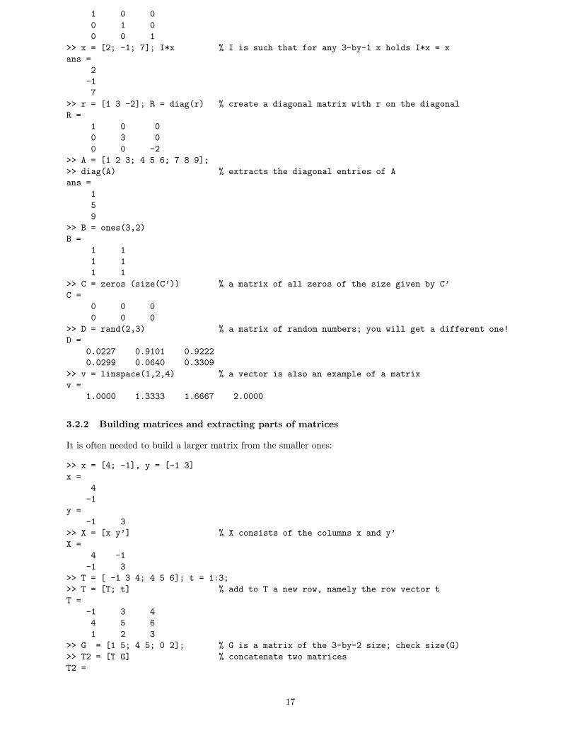
3.2.2 Building matrices and extracting parts of matrices

It is often needed to build a larger matrix from the smaller ones:

>> x = [4; -1], y = [-1 3]

x =

4

-1

y =

-1 3

>> X = [x y’] % X consists of the columns x and y’

X =

4 -1

-1 3

>> T = [ -1 3 4; 4 5 6]; t = 1:3;

>> T = [T; t] % add to T a new row, namely the row vector t

T =

-1 3 4

4 5 6

1 2 3

>> G = [1 5; 4 5; 0 2]; % G is a matrix of the 3-by-2 size; check size(G)

>> T2 = [T G] % concatenate two matrices

T2 =

17

-1 3 4 1 5

4 5 6 4 5

1 2 3 0 2

>> T3 = [T; G ones(3,1)] % G is 3-by-2, T is 3-by-3

T3 =

-1 3 4

4 5 6

1 2 3

1 5 1

4 5 1

0 2 1

>> T3 = [T; G’]; % this is also possible; what do you get here?

>> [G’ diag(5:6); ones(3,2) T] % you can concatenate many matrices

ans =

1 4 0 5 0

5 5 2 0 6

1 1 -1 3 4

1 1 4 5 6

1 1 1 2 3

A part can be extract from a matrix in a similar way as from a vector. Each element in the matrix is indexedby a row and a column to which it belongs. Mathematically, the element from the i-th row and the j-thcolumn of the matrix A is denoted by Aij ; Matlab provides the A(i,j) notation.

>> A = [1:3; 4:6; 7:9]

A =

1 2 3

4 5 6

7 8 9

>> A(1,2), A(2,3), A(3,1)

ans =

2

ans =

6

ans =

7

>> A(4,3) % this is not possible: A is a 3-by-3 matrix!

??? Index exceeds matrix dimensions.

>> A(2,3) = A(2,3) + 2*A(1,1) % change the value of A(2,3)

A =

1 2 3

4 5 8

7 8 9

It is easy to extend a matrix automatically. For the matrix A it can be done e.g. as follows:

>> A(5,2) = 5 % assign 5 to the position (5,2); the uninitialized

A = % elements become zeros

1 2 3

4 5 8

7 8 9

0 0 0

0 5 0

If needed, the other zero elements of the matrix A can be also defined, by e.g.:

>> A(4,:) = [2, 1, 2]; % assign vector [2, 1, 2] to the 4th row of A

>> A(5,[1,3]) = [4, 4]; % assign: A(5,1) = 4 and A(5,3) = 4

>> A % how does the matrix A look like now?

Different parts of the matrix A can be now extracted:

18

>> A(3,:) % extract the 3rd row of A

ans =

7 8 9

>> A(:,2) % extract the 2nd column of A

ans =

2

5

8

1

5

>> A(1:2,:) % extract the rows 1st and 2nd of A

ans =

1 2 3

4 5 8

>> A([2,5],1:2) % extract a part of A

ans =

4 5

4 5

As you have seen in the examples above, it is possible to manipulate (groups of) matrix-elements. Thecommands are shortly explained in Table 3.

The concept of an empty matrix [] is also very useful in Matlab. For instance, a few columns or rows canbe removed from a matrix by assigning an empty matrix to it. Try for example:

>> C = [1 2 3 4; 5 6 7 8; 1 1 1 1];

>> D = C; D(:,2) = [] % now a copy of C is in D; remove the 2nd column of D

>> C ([1,3],:) = [] % remove the rows 1 and 3 from C

Exercise 11.Clear all variables. Define the matrix: A = [1:4; 5:8; 1 1 1 1]. Predict and check the result of:

• x = A(:, 3)

• B = A(1 : 3, 2 : 2)

• A(1, 1) = 9 + A(2, 3)

• A(2 : 3, 1 : 3) = [0 0 0; 0 0 0]

• A(2 : 3, 1 : 2) = [1 1; 3 3]

• y = A(3 : 3, 1 : 4)

• A = [A; 2 1 7 7; 7 7 4 5]

• C = A([1, 3], 2)

• D = A([2, 3, 5], [1, 3, 4])

• D(2, :) = [ ]�

Exercise 12.Define the matrices: T = [ 3 4; 1 8; -4 3]; A = [diag(-1:2:3) T; -4 4 1 2 1]. Perform the followingoperations on the matrix A:• extract a vector consisting of the 2nd and 4th elements of the 3rd row

• find the minimum of the 3rd column

• find the maximum of the 2nd row

• compute the sum of the 2nd column

• compute the mean of the 1st and 4th rows

• extract the submatrix consisting of the 1st and 3rd rows and all columns

• extract the submatrix consisting of the 1st and 2nd rows and the 3rd, 4th and 5th columns

• compute the total sum of the 1st and 2nd rows

• add 3 to all elements of the 2nd and 3rd columns�

Exercise 13.Let A = [2 4 1; 6 7 2; 3 5 9]. Provide the commands which:• assign the first row of A to a vector x;

• assign the last 2 rows of A to a vector y;

• add up the columns of A;

• add up the rows of A;

• compute the standard error of the mean of each column of A (i.e. the standard deviation divided by thesquare root of the number of elements used to compute the mean).

�

19

Exercise 14.Let A = [2 7 9 7; 3 1 5 6; 8 1 2 5]. Explain the results or perform the following commands:

• A′

• A(1, :)′

• A(:, [14])

• A([23], [31])

• reshape (A, 2, 6)

• A(:)

• flipud (A)

• fliplr (A)

• [A A(end, :)]

• [A; A(1 : 2, :)]

• sum (A)

• sum (A′)

• mean (A)

• mean (A′)

• sum (A, 2)

• mean (A, 2)

• min (A)

• max (A′)

• min (A(:, 4))

• [min(A)′ max(A)′]

• max (min(A))

• [[A; sum (A)] [sum (A, 2); sum (A(:))]]

• assign the even-numbered columns of A to an array B

• assign the odd-numbered rows to an array C

• convert A into a 4-by-3 array

• compute the reciprocal of each element of A

• compute the square-root of each element of A

• remove the second column of A

• add a row of all 1’s at the beginning and at the end

• swap the 2nd row and the last row

�

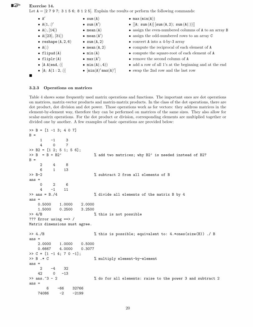
3.2.3 Operations on matrices

Table 4 shows some frequently used matrix operations and functions. The important ones are dot operationson matrices, matrix-vector products and matrix-matrix products. In the class of the dot operations, there aredot product, dot division and dot power. Those operations work as for vectors: they address matrices in theelement-by-element way, therefore they can be performed on matrices of the same sizes. They also allow forscalar-matrix operations. For the dot product or division, corresponding elements are multiplied together ordivided one by another. A few examples of basic operations are provided below:

>> B = [1 -1 3; 4 0 7]

B =

1 -1 3

4 0 7

>> B2 = [1 2; 5 1; 5 6];

>> B = B + B2’ % add two matrices; why B2’ is needed instead of B2?

B =

2 4 8

6 1 13

>> B-2 % subtract 2 from all elements of B

ans =

0 2 6

4 -1 11

>> ans = B./4 % divide all elements of the matrix B by 4

ans =

0.5000 1.0000 2.0000

1.5000 0.2500 3.2500

>> 4/B % this is not possible

??? Error using ==> /

Matrix dimensions must agree.

>> 4./B % this is possible; equivalent to: 4.*ones(size(B)) ./ B

ans =

2.0000 1.0000 0.5000

0.6667 4.0000 0.3077

>> C = [1 -1 4; 7 0 -1];

>> B .* C % multiply element-by-element

ans =

2 -4 32

42 0 -13

>> ans.^3 - 2 % do for all elements: raise to the power 3 and subtract 2

ans =

6 -66 32766

74086 -2 -2199

20

>> ans ./ B.^2 % element-by-element division

ans =

0.7500 -1.0312 63.9961

342.9907 -2.0000 -1.0009

>> r = [1 3 -2]; r * B2 % this is a legal operation: r is a 1-by-3 matrix and B2 is

ans = % 3-by-2 matrix; B2 * r is an illegal operation

6 -7

Concerning the matrix-vector and matrix-matrix products, two things should be reminded. First, an n × kmatrix A (having n rows and k columns) can be multiply by a k × 1 (column) vector x, resulting in a column

n × 1 vector y, i.e.: A x = y such that yi =∑k

p=1 Aip xp. Multiplying a 1 × n (row) vector x by a matrix A,results in a 1× k (row) vector y. Secondly, an n× k matrix A can be multiply by a matrix B, only if B hask rows, i.e. B is k ×m (m is arbitrary). As a result, you get n ×m matrix C, such that A B = C, where

Cij =∑k

p=1 Aip Bpj .

>> b = [1 3 -2];

>> B = [1 -1 3; 4 0 7]

B =

1 -1 3

4 0 7

>> b * B % not possible: b is 1-by-3 and B is 2-by-3

??? Error using ==> *

Inner matrix dimensions must agree.

>> b * B’ % this is possible: a row vector multiplied by a matrix

ans =

-8 -10

>> B’ *ones(2,1)

ans =

5

-1

10

>> C = [3 1; 1 -3];

>> C * B

ans =

7 -3 16

-11 -1 -18

>> C.^3 % this is element-by-element power

ans =

27 1

1 -27

>> C^3 % this is equivalent to C*C*C

ans =

30 10

10 -30

>> ones(3,4)./4 * diag(1:4)

ans =

0.2500 0.5000 0.7500 1.0000

0.2500 0.5000 0.7500 1.0000

0.2500 0.5000 0.7500 1.0000

Exercise 15.Perform all operations from Table 4, using chosen matrices A and B, vector v and scalars k, a, b, n, and m. �

Exercise 16.Let A be a square matrix.

1. Create a matrix B, whose elements are the same as those of A except the entries on the main diagonal.The diagonal of B should consist of 1s.

2. Create a tridiagonal matrix T, whose three diagonal are taken from the matrix A. Hint: you may use thecommands triu and tril.

�

21

Symbol Color Symbol Line style

r red ., o point, circleg green * starb blue x, + x-mark, plusy yellow - solid linem magenta -- dash linec cyan : dot linek black -. dash-dot line

Table 5: Plot colors and styles.

Exercise 17.Given the vectors x = [1 3 7], y = [2 4 2] and the matrices A = [3 1 6; 5 2 7], B = [1 4; 7 8; 2 2], determinewhich of the following statements will correctly execute (and if not, try to understand why) and provide theresult:

• x + y

• x + A

• x′ + y

• A− [x′ y′]

• [x; y] + A

• [x; y′]

• [x; y]

• A− 3

• A + B

• B′ + A

• B ∗ A• A. ∗ B• A′. ∗ B• 2 ∗ B• 2. ∗ B

• B./x′

• B./[x′ x′]

• 2/A

• ones(1, 3) ∗ A• ones(1, 3) ∗ B

�

Exercise 18.Let A be a random 5 × 5 matrix, and b a random 5 × 1 vector. Given that Ax = b, try to find x (look at

76-79Table 4). Explain what is the difference between the operators \, / and the command inv. Having found x,check whether Ax − b is close to a zero vector. �

Exercise 19.Let A = ones(6) + eye(6). Normalize columns of the matrix A so that all columns of the resulting matrix,say B, have the Euclidean norm (length) equal to 1. Then, find the angles between consecutive columns of thematrix B. �

Exercise 20.Find two 2× 2 matrices A and B which fulfill that A. ∗ B 6= A ∗ B. Then, try to find all 2× 2 matrices A andB for which the following holds: A. ∗ B = A ∗ B (make use one or more from the following operations: /, \, orthe command inv). �

4 Visualization

Matlab can be used to visualize the results of an experiment. Therefore, you should define variables, each ofthem containing all values of one parameter to plot.

4.1 Simple plots

With the command plot, a graphical display can be made. For a vector y, plot(y) draws the points [1, y(1)],184 [2, y(2)], . . ., [n, y(n)] and connects them with a straight line. plot(x,y) does the same for the points

[x(1), y(1)], [x(2), y(2)], . . . , [x(n), y(n)]. Note that x and y have to be both either row or column vectorsof the same length (i.e. the number of elements).

The commands loglog, semilogx and semilogy are similar to plot, except that they use either one or twologarithmic axes.

Exercise 21.Type the following commands after predicting the result:

>> x = 0:10;

>> y = 2.^x; % this is the same as y = [1 2 4 8 16 32 64 128 256 512 1024]

>> plot(x,y) % to get a graphic representation

>> semilogy(x,y) % to make the y-axis logarithmic

22

As you can see, the same figure is used for both plot commands. The previous function is removed as soonas the next is displayed. The command figure gives you an extra figure. Repeat the previous commands,but generate a new figure before plotting the second function, so that you can see both functions in separatewindows. You can also switch back to a figure using figure(n), where n is its number. �

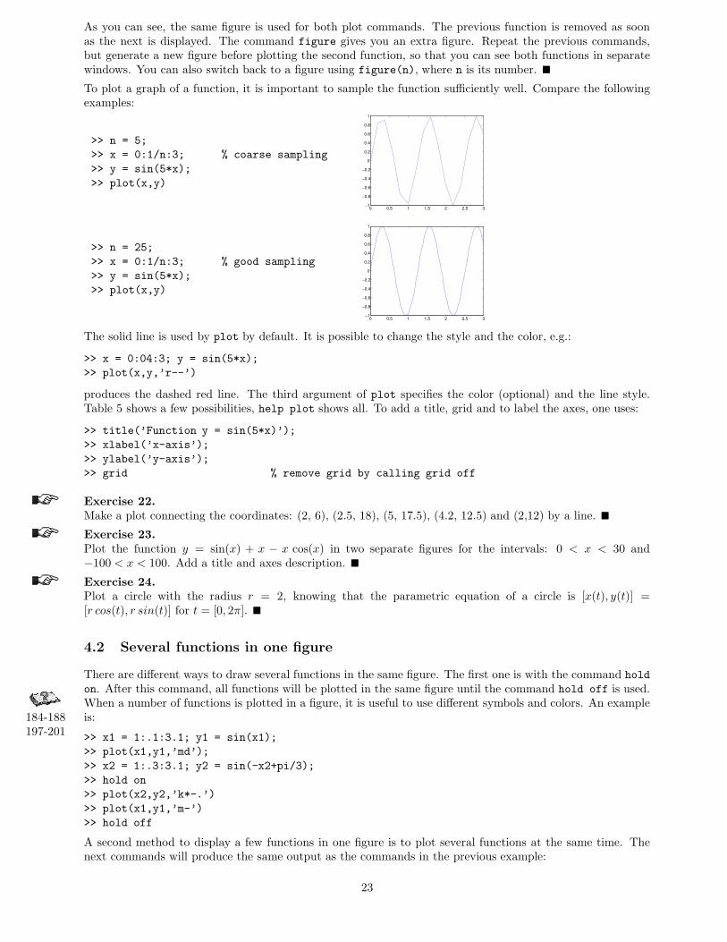
To plot a graph of a function, it is important to sample the function sufficiently well. Compare the followingexamples:

>> n = 5;

>> x = 0:1/n:3; % coarse sampling

>> y = sin(5*x);

>> plot(x,y)

0 0.5 1 1.5 2 2.5 3−1

−0.8

−0.6

−0.4

−0.2

0

0.2

0.4

0.6

0.8

1

>> n = 25;

>> x = 0:1/n:3; % good sampling

>> y = sin(5*x);

>> plot(x,y)

0 0.5 1 1.5 2 2.5 3−1

−0.8

−0.6

−0.4

−0.2

0

0.2

0.4

0.6

0.8

1

The solid line is used by plot by default. It is possible to change the style and the color, e.g.:

>> x = 0:04:3; y = sin(5*x);

>> plot(x,y,’r--’)

produces the dashed red line. The third argument of plot specifies the color (optional) and the line style.Table 5 shows a few possibilities, help plot shows all. To add a title, grid and to label the axes, one uses:

>> title(’Function y = sin(5*x)’);

>> xlabel(’x-axis’);

>> ylabel(’y-axis’);

>> grid % remove grid by calling grid off

Exercise 22.Make a plot connecting the coordinates: (2, 6), (2.5, 18), (5, 17.5), (4.2, 12.5) and (2,12) by a line. �

Exercise 23.Plot the function y = sin(x) + x − x cos(x) in two separate figures for the intervals: 0 < x < 30 and−100 < x < 100. Add a title and axes description. �

Exercise 24.Plot a circle with the radius r = 2, knowing that the parametric equation of a circle is [x(t), y(t)] =[r cos(t), r sin(t)] for t = [0, 2π]. �

4.2 Several functions in one figure

There are different ways to draw several functions in the same figure. The first one is with the command hold

on. After this command, all functions will be plotted in the same figure until the command hold off is used.When a number of functions is plotted in a figure, it is useful to use different symbols and colors. An example

184-188197-201

is:

>> x1 = 1:.1:3.1; y1 = sin(x1);

>> plot(x1,y1,’md’);

>> x2 = 1:.3:3.1; y2 = sin(-x2+pi/3);

>> hold on

>> plot(x2,y2,’k*-.’)

>> plot(x1,y1,’m-’)

>> hold off

A second method to display a few functions in one figure is to plot several functions at the same time. Thenext commands will produce the same output as the commands in the previous example:

23

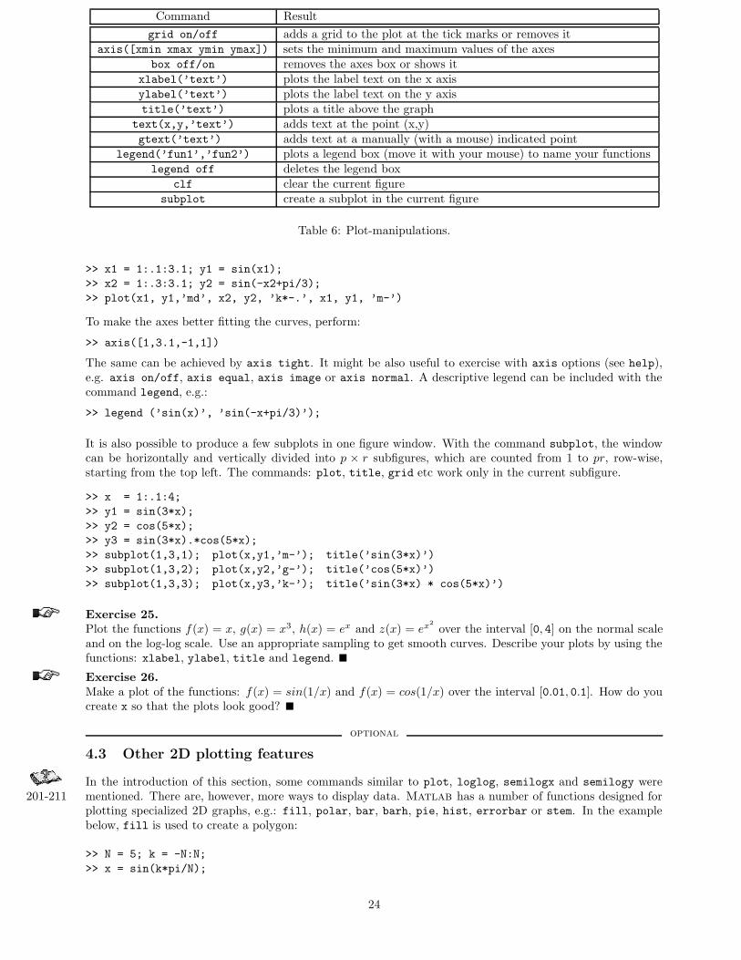
Command Result

grid on/off adds a grid to the plot at the tick marks or removes itaxis([xmin xmax ymin ymax]) sets the minimum and maximum values of the axes

box off/on removes the axes box or shows itxlabel(’text’) plots the label text on the x axisylabel(’text’) plots the label text on the y axistitle(’text’) plots a title above the graph

text(x,y,’text’) adds text at the point (x,y)gtext(’text’) adds text at a manually (with a mouse) indicated point

legend(’fun1’,’fun2’) plots a legend box (move it with your mouse) to name your functionslegend off deletes the legend box

clf clear the current figuresubplot create a subplot in the current figure

Table 6: Plot-manipulations.

>> x1 = 1:.1:3.1; y1 = sin(x1);

>> x2 = 1:.3:3.1; y2 = sin(-x2+pi/3);

>> plot(x1, y1,’md’, x2, y2, ’k*-.’, x1, y1, ’m-’)

To make the axes better fitting the curves, perform:

>> axis([1,3.1,-1,1])

The same can be achieved by axis tight. It might be also useful to exercise with axis options (see help),e.g. axis on/off, axis equal, axis image or axis normal. A descriptive legend can be included with thecommand legend, e.g.:

>> legend (’sin(x)’, ’sin(-x+pi/3)’);

It is also possible to produce a few subplots in one figure window. With the command subplot, the windowcan be horizontally and vertically divided into p × r subfigures, which are counted from 1 to pr, row-wise,starting from the top left. The commands: plot, title, grid etc work only in the current subfigure.

>> x = 1:.1:4;

>> y1 = sin(3*x);

>> y2 = cos(5*x);

>> y3 = sin(3*x).*cos(5*x);

>> subplot(1,3,1); plot(x,y1,’m-’); title(’sin(3*x)’)

>> subplot(1,3,2); plot(x,y2,’g-’); title(’cos(5*x)’)

>> subplot(1,3,3); plot(x,y3,’k-’); title(’sin(3*x) * cos(5*x)’)

Exercise 25.Plot the functions f(x) = x, g(x) = x3, h(x) = ex and z(x) = ex2

over the interval [0, 4] on the normal scaleand on the log-log scale. Use an appropriate sampling to get smooth curves. Describe your plots by using thefunctions: xlabel, ylabel, title and legend. �

Exercise 26.Make a plot of the functions: f(x) = sin(1/x) and f(x) = cos(1/x) over the interval [0.01, 0.1]. How do youcreate x so that the plots look good? �

optional

4.3 Other 2D plotting features

In the introduction of this section, some commands similar to plot, loglog, semilogx and semilogy were201-211 mentioned. There are, however, more ways to display data. Matlab has a number of functions designed for

plotting specialized 2D graphs, e.g.: fill, polar, bar, barh, pie, hist, errorbar or stem. In the examplebelow, fill is used to create a polygon:

>> N = 5; k = -N:N;

>> x = sin(k*pi/N);

24

>> y = cos(k*pi/N); % x and y - vertices of the polygon to be filled

>> fill(x,y,’g’)

>> axis square

>> text(-0.45,0,’I am a green polygon’)

Exercise 27.To get an impression of other visualizations, type the following commands and describe the result (note thatthe command figure creates a new figure window):

>> figure % bar plot of a bell shaped curve

>> x = -2.9:0.2:2.9;

>> bar(x,exp(-x.*x));

>> figure % stairstep plot of a sine wave

>> x = 0:0.25:10;

>> stairs(x,sin(x));

>> figure % errorbar plot

>> x = -2:0.1:2;

>> y = erf(x); % error function; check help if you are interested

>> e = rand(size(x)) / 10;

>> errorbar (x,y,e);

>> figure

>> r = rand(5,3);

>> subplot(1,2,1); bar(r,’grouped’) % bar plot

>> subplot(1,2,2); bar(r,’stacked’)

>> figure

>> x = randn(200,1); % normally distributed random numbers

>> hist(x,15) % histogram with 15 bins

�

end optional

4.4 Printing

Before printing a figure, you might want to add some information, such as a title, or change somewhat in the189-196 lay-out. Table 6 shows some of the commands that can be used.

Exercise 28.Plot the functions y1 = sin(4x), y2 = x cos(x), y3 = (x + 1)−1√x for x = 1 : 0.25 : 10; and a single point(x, y) = (4, 5) in one figure. Use different colors and styles. Add a legend, labels for both axes and a title.Add also a text to the single point saying: ’single point’. Change the minimum and maximum values of theaxes such that one can look at the function y3 in more detail. �

When you like the displayed figure, you can print it to paper. The easiest way is to click on File in themenu-bar and to choose Print. If you click OK in the print window, your figure will be sent to the printerindicated there.

There exists also a print command, which can be used to send a figure to a printer or output it to a file. Youcan optionally specify a print device (i.e. an output format such as tiff or postscript) and options that controlvarious characteristics of the printed file (i.e., which Figure to print etc). You can also print to a file if youspecify the file name. If you do not provide an extension, print adds one. Since they are many parametersthey will not be explained here (check help print to learn more). Instead, try to understand the examples:

>> print -dwinc % print the current Figure to the current printer in color

>> print -f1 -deps myfile.eps % print Figure no.1 to the file myfile.eps in black

>> print -f1 -depsc myfilec.eps % print Figure no.1 to the file myfilec.eps in color

>> print -dtiff myfile1.tiff % print the current Figure to the file myfile1.tiff

>> print -dpsc myfile1c.ps % print the current Figure to the file myfile1.ps in color

>> print -f2 -djpeg myfile2 % print Figure no.2 to the file myfile2.jpg

Exercise 29.Practise with printing (especially to a file) the figures from previous exercises. �

25

4.5 3D line plots

The command plot3 to plot lines in 3D is equivalent to the command plot in 2D. The format is the same214 as for plot, it is, however, extended by an extra coordinate. An example is plotting the curve r defined

parametrically as r(t) = [t sin(t), t cos(t), t] over the interval [−10 π, 10 π].>> t = linspace(-10*pi,10*pi,200);

>> plot3(t.*sin(t), t.*cos(t), t, ’md-’); % plot the curve in magenta

>> title(’Curve r(t) = [t sin(t), t cos(t), t]’);

>> xlabel(’x-axis’); ylabel(’y-axis’); zlabel(’z-axis’);

>> grid

Exercise 30.Make a 3D smooth plot of the curve defined parametrically as: [x(t), y(t), z(t)] = [sin(t), cos(t), sin2(t)] fort = [0, 2π]. Plot the curve in green, with the points marked by circles. Add a title, description of axes and thegrid. You can rotate the image by clicking Tools at the Figure window and choosing the Rotate 3D optionor by typing rotate3D at the prompt. Then by clicking at the image and dragging your mouse you can rotatethe axes. Exercise with this option. �

4.6 Plotting surfaces

Matlab provides a number of commands to plot 3D data. A surface is defined by a function f(x, y), where216-220 for each pair of (x, y), the height z is computed as z = f(x, y). To plot a surface, a rectangular domain of the

(x, y)-plane should be sampled. The mesh (or grid) is constructed by the use of the command meshgrid asfollows:

>> [X, Y] = meshgrid (-1:.5:1, 0:.5:2)

X =

-1.0000 -0.5000 0 0.5000 1.0000

-1.0000 -0.5000 0 0.5000 1.0000

-1.0000 -0.5000 0 0.5000 1.0000

-1.0000 -0.5000 0 0.5000 1.0000

-1.0000 -0.5000 0 0.5000 1.0000

Y =

0 0 0 0 0

0.5000 0.5000 0.5000 0.5000 0.5000

1.0000 1.0000 1.0000 1.0000 1.0000

1.5000 1.5000 1.5000 1.5000 1.5000

2.0000 2.0000 2.0000 2.0000 2.0000

The domain [−1, 1] × [0, 2] is now sampled with 0.5 in both directions and it is described by points[X(i, j), Y (i, j)]. To plot a smooth surface, the chosen domain should be sampled in a more dense way.To plot a surface, the command mesh or surf can be used:

>> [X,Y] = meshgrid(-1:.05:1, 0:.05:2);

>> Z = sin(5*X) .* cos(2*Y);

>> mesh(X,Y,Z);

>> title (’Function z = sin(5x) * cos(2y)’)

You can also try waterfall instead of mesh.

Exercise 31.Produce a nice graph which demonstrates as clearly as possible the behavior of the function f(x, y) = x y2

x2+y4

near the point (0, 0). Note that the sampling around this points should be dense enough. �

Exercise 32.Plot a sphere, which is parametrically defined as [x(t, s), y(t, s), z(t, s)] = [cos(t) cos(s), cos(t) sin(s), sin(t)]for t, s = [0, 2 π] (use surf). Make first equal axes, then remove them. Use shading interp to remove blacklines (use shading faceted to restore the original picture). �

Exercise 33.Plot the parametric function of r and θ: [x(r, θ), y(r, θ), z(r, θ)] = [r cos(θ), r sin(θ), sin(6 cos(r)−nθ)]. Choosen to be constant. Observe, how the graph changes depending on different n. �

The Matlab function peaks is a function of two variables, obtained by translating and scaling Gaussiandistributions. Perform, for instance:

26

>> [X,Y,Z] = peaks; % create values for plotting the function

>> surf(X,Y,Z); % plot the surface

>> figure

>> contour (X,Y,Z,30); % draw the contour lines in 2D

>> colorbar % adds a bar with colors corresponding to the z-axis

>> title(’2D-contour of PEAKS’);

>> figure

>> contour3(X,Y,Z,30); % draw the contour lines in 3D

>> title(’3D-contour of PEAKS’);

>> pcolor(X,Y,Z); % z-values are mapped to the colors and presented as

% a ’checkboard’ plot; similar to contour

Use close all to close all figures and start a new task (or use close 1 to close Figure no.1 etc). Use colormap231-236 to define different colors for plotting.

To locate e.g. the minimum value of the peaks function on the grid, you can proceed as follows:

>> [mm,I] = min(Z); % a row vector of the min. elements from each column

>> % I is a vector of corresponding

>> [Zmin, j] = min (mm); % Zmin is the minimum value, j is the index

% Zmin is the value of Z(I(j),j)

>> xpos = X(I(j),j); %

>> ypos = Y(I(j),j); % position of the minimum value

>> contour (X,Y,Z,25);

>> xlabel(’x-axis’); ylabel(’y-axis’);

>> hold on

>> plot(xpos(1),ypos,’*’);

>> text(xpos(1)+0.1,ypos,’Minimum’);

>> hold off

It is also possible to combine two or more plots into one figure. For instance:

>> surf(peaks(25)+6); % move the z-values with the vector [0,0,6]

>> hold on

>> pcolor(peaks(25));

Exercise 34.Plot the surface f(x, y) = x y e−x2−y2

over the domain [−2, 2]× [−2, 2]. Find the values and the locations ofthe minima and maxima of this function. �

optional

4.7 Animations

A sequence of graphs can be put in motion in Matlab(the version should be at least 5.0), i.e. you can makea movie using Matlab graphics tools. To learn how to create a movie, analyze first the script below whichshows the plots of f(x) = sin(nx) over the interval [0, 2π] and = 1, . . . , 5:

N = 5;

M = moviein(N);

x = linspace (0,2*pi);

for n=1:N

plot (x,cos(n*x),’r-’);

xlabel(’x-axis’)

if n > 1,

ss = strcat(’cos(’,num2str(n),’x)’);

else

ss = ’cos(x)’;

end

ylabel(ss)

title(’Cosine functions cos(nx)’,’FontSize’,12)

axis tight

27

grid

M(:,n) = getframe;

pause(1.8)

end

movie(M) % this plays a quick movie

Here, a for-loop construction has been used to create the movie frames. You will learn more on loops insection 5.3. Also the command strcat has been used to concatenate strings. Use help to understand or learnmore from section 8.1.

Play this movie to get acquainted. Five frames are first displayed and at the end, the same frames are playedagain faster. Command moviein, with an integral parameter, tells Matlab that a movie consisting of N

frames is going to be created. Consecutive frames are generated inside the loop. Via the command getframe

each frame is stored in the column of the matrix m. The command movie(M) plays the movie just createdand saved in columns of the matrix M. Note that to create a movie requires quite some memory. It might beuseful to clear M from the workspace later on.

Exercise 35.Write a script that makes a movie consisting of 5 frames of the surface f(x, y) = sin(nx) sin(ky) over thedomain [0, 2π]× [0, 2π] and n = 1 : 5. Add a title, description of axes and shading. �

end optional

5 Control flow

A control flow structure is a block of commands that allows conditional code execution and making loops.

5.1 Logical and relational operators

To use control flow commands, it is necessary to perform operations that result in logical values: TRUE or88-91 FALSE. In Matlab the result of a logical operation is 1 if it is true and 0 if it is false. Table 7 shows the

relational and logical operations3. Another way to get to know more about them is to type help relop. Therelational operators <, <=, >, >=, == and ~= can be used to compare two arrays of the same size or anarray to a scalar. The logical operators &, | and ~ allow for the logical combination or negation of relationaloperators. In addition, three functions are also available: xor, any and all (use help to find out more).

Command Result

a = (b > c) a is 1 if b is larger than c. Similar are: <, >= and <=

a = (b == c) a is 1 if b is equal to c

a = (b ~= c) a is 1 if b is not equal ca = ~b logical complement: a is 1 if b is 0a = (b & c) logical AND: a is 1 if b = TRUE AND c = TRUEa = (b | c) logical OR: a is 1 if b = TRUE OR c = TRUE

Table 7: Relational and logical operations.

Important: The logical & and | have the equal precedence in Matlab, which means that those operatorsassociate from left to right. A common situation is:

>> b = 10;

>> 1 | b > 0 & 0

ans =

0

>> (1 | b > 0) & 0 % this indicates the same as above

ans =

0

>> 1 | (b > 0 & 0)

ans =

1

3”equal to” in the table on page 88 of ”The Student Edition of Matlab” must be ”==” instead of ”=”

28

This shows that you should always use brackets to indicate in which way the operators should be evaluated.

The introduction of the logical data type has forced some changes in the use of non-logical 0-1 vectors asindices for subscripting. You can see the differences by executing the following commands that attempt toextract the elements of y that correspond to either the odd or even elements of x, assuming that x and y aretwo vectors of the same length.

• y (rem (x, 2)) vs. y (logical (rem (x, 2))) % odd elements

• y (~rem (x, 2)) vs. y (~logical (rem (x, 2))) % even elements

Exercise 36.Exercise with logical and relational operators:

1. Predict and check the result of each of the operations of Table 7 for b = 0 and c = -1.

2. Predict and check the result of each logical operator for b = [2 31 -40 0] and c = 0.

3. Define two random vectors (randn(1,7)) and perform all logical operations, including xor, any and all.�

Exercise 37.Exercise with logical and relational operators:

1. Let x = [1 5 2 8 9 0 1] and y = [5 2 2 6 0 0 2]. Execute and explain the results of the following com-mands:

• x > y

• y < x

• x == y

• x <= y

• y >= x

• x | y

• x & (~y)• (x > y) | (y < x)• (x > y) & (y < x)

2. Let x = 1 : 10 and y = [3 5 6 1 8 2 9 4 0 7]. The exercises here show the techniques of logical-indexing.Execute and interpret the results of the following commands:

• (x > 3) & (x < 8)• x (x > 5)• y (x <= 4)

• x ((x < 2) | (x >= 8))• y ((x < 2) | (x >= 8))• x (y < 0)

�

Exercise 38.Let x = [3 16 9 12 -1 0 -12 9 6 1]. Provide the command(s) that will:

• set the positive values of x to zero;

• set values that are multiples of 3 to 3 (make use of rem);

• multiply the even values of x by 5;

• extract the values of x that are greater than 10 into a vector called y;

• set the values in x that are less than the mean to 0;

• set the values in x that are above the mean to their difference from the mean.�

Exercise 39.Execute the following commands and try to understand how z is defined.

>> hold on

>> x = -3:0.05:3; y = sin(3*x);

>> subplot(1,2,1); plot(x,y); axis tight

>> z = (y < 0.5) .* y;

>> subplot(1,2,2); plot(x,y,’r:’); plot(x,z,’r’); axis tight

>> hold off�

Before moving on, check whether you now understand the following relations:

>> a = randperm(10); % random permutation

>> b = 1:10;

>> b - (a <= 7) % subtracts from b a 0-1 vector, taking 1 for a <= 7 and 0 otherwise

>> (a >= 2) & (a < 4) % returns ones at positions where 2 <= a < 4

>> ~(b > 4) % returns ones at positions where b <= 4

>> (a == b) | b == 3 % returns ones at positions where a is equal to b or b is equal to 3

>> any(a > 5) % returns 1 when ANY of the a elements are larger than 5

>> any(b < 5 & a > 8) % returns 1 when there in the evaluated expression

>> % (b < 5 & a > 8) appears at least one 1

>> all(b > 2) % returns 1 when ALL b elements are larger than 2

29

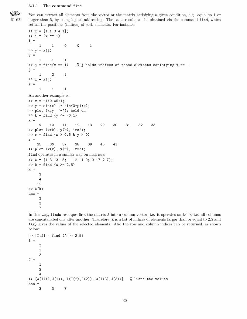
5.1.1 The command find

You can extract all elements from the vector or the matrix satisfying a given condition, e.g. equal to 1 or61-62 larger than 5, by using logical addressing. The same result can be obtained via the command find, which

return the positions (indices) of such elements. For instance:

>> x = [1 1 3 4 1];

>> i = (x == 1)

i =

1 1 0 0 1

>> y = x(i)

y =

1 1 1

>> j = find(x == 1) % j holds indices of those elements satisfying x == 1

j =

1 2 5

>> z = x(j)

z =

1 1 1

An another example is:

>> x = -1:0.05:1;

>> y = sin(x) .* sin(3*pi*x);

>> plot (x,y, ’-’); hold on

>> k = find (y <= -0.1)

k =

9 10 11 12 13 29 30 31 32 33

>> plot (x(k), y(k), ’ro’);

>> r = find (x > 0.5 & y > 0)

r =

35 36 37 38 39 40 41

>> plot (x(r), y(r), ’r*’);

find operates in a similar way on matrices:

>> A = [1 3 -3 -5; -1 2 -1 0; 3 -7 2 7];

>> k = find (A >= 2.5)

k =

3

4

12

>> A(k)

ans =

3

3

7

In this way, finds reshapes first the matrix A into a column vector, i.e. it operates on A(:), i.e. all columnsare concatenated one after another. Therefore, k is a list of indices of elements larger than or equal to 2.5 andA(k) gives the values of the selected elements. Also the row and column indices can be returned, as shownbelow:

>> [I,J] = find (A >= 2.5)

I =

3

1

3

J =

1

2

4

>> [A(I(1),J(1)), A(I(2),J(2)), A(I(3),J(3))] % lists the values

ans =

3 3 7

30

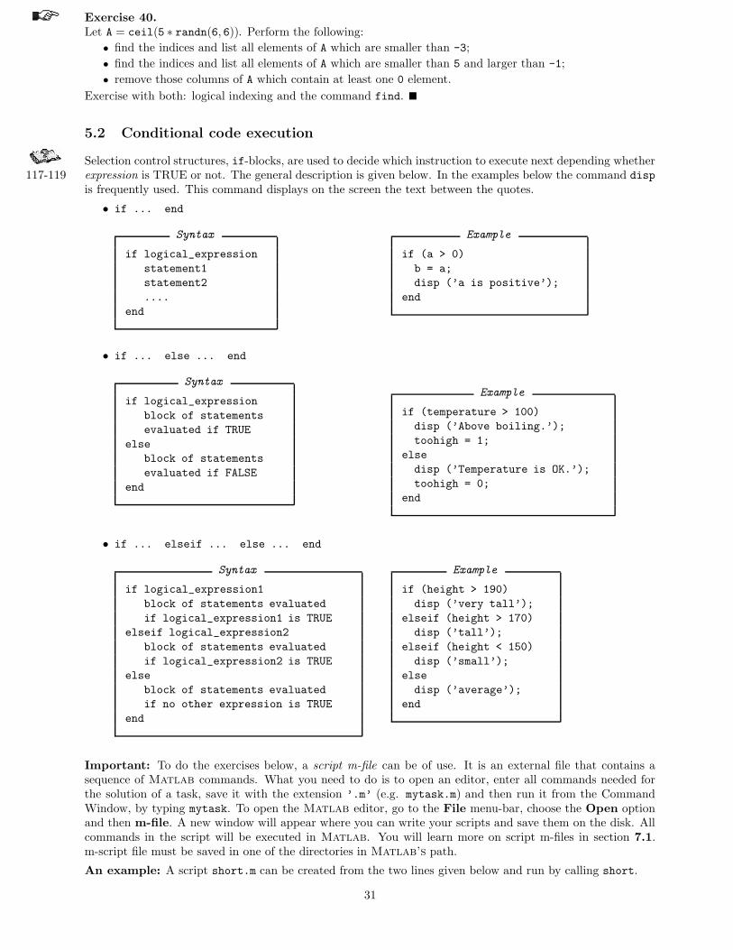
Exercise 40.Let A = ceil(5 ∗ randn(6, 6)). Perform the following:

• find the indices and list all elements of A which are smaller than -3;

• find the indices and list all elements of A which are smaller than 5 and larger than -1;

• remove those columns of A which contain at least one 0 element.

Exercise with both: logical indexing and the command find. �

5.2 Conditional code execution

Selection control structures, if-blocks, are used to decide which instruction to execute next depending whether117-119 expression is TRUE or not. The general description is given below. In the examples below the command disp

is frequently used. This command displays on the screen the text between the quotes.

• if ... end

Syntax

if logical_expression

statement1

statement2

....

end

Example

if (a > 0)

b = a;

disp (’a is positive’);

end

• if ... else ... end

Syntax

if logical_expression

block of statements

evaluated if TRUE

else

block of statements

evaluated if FALSE

end

Example

if (temperature > 100)

disp (’Above boiling.’);

toohigh = 1;

else

disp (’Temperature is OK.’);

toohigh = 0;

end

• if ... elseif ... else ... end

Syntax

if logical_expression1

block of statements evaluated

if logical_expression1 is TRUE

elseif logical_expression2

block of statements evaluated

if logical_expression2 is TRUE

else

block of statements evaluated

if no other expression is TRUE

end

Example

if (height > 190)

disp (’very tall’);

elseif (height > 170)

disp (’tall’);

elseif (height < 150)

disp (’small’);

else

disp (’average’);

end

Important: To do the exercises below, a script m-file can be of use. It is an external file that contains asequence of Matlab commands. What you need to do is to open an editor, enter all commands needed forthe solution of a task, save it with the extension ’.m’ (e.g. mytask.m) and then run it from the CommandWindow, by typing mytask. To open the Matlab editor, go to the File menu-bar, choose the Open optionand then m-file. A new window will appear where you can write your scripts and save them on the disk. Allcommands in the script will be executed in Matlab. You will learn more on script m-files in section 7.1.m-script file must be saved in one of the directories in Matlab’s path.

An example: A script short.m can be created from the two lines given below and run by calling short.

31

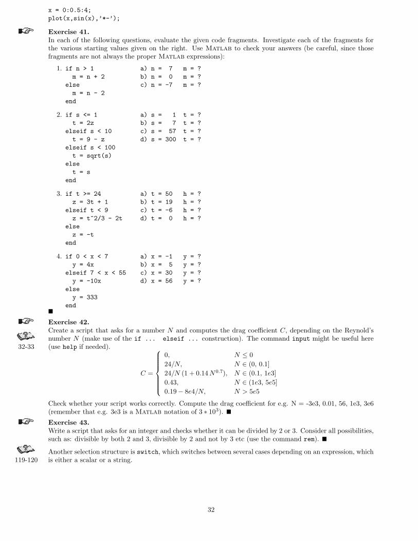
x = 0:0.5:4;

plot(x,sin(x),’*-’);

Exercise 41.In each of the following questions, evaluate the given code fragments. Investigate each of the fragments forthe various starting values given on the right. Use Matlab to check your answers (be careful, since thosefragments are not always the proper Matlab expressions):

1. if n > 1 a) n = 7 m = ?

m = n + 2 b) n = 0 m = ?

else c) n = -7 m = ?

m = n - 2

end

2. if s <= 1 a) s = 1 t = ?

t = 2z b) s = 7 t = ?

elseif s < 10 c) s = 57 t = ?

t = 9 - z d) s = 300 t = ?

elseif s < 100

t = sqrt(s)

else

t = s

end

3. if t >= 24 a) t = 50 h = ?

z = 3t + 1 b) t = 19 h = ?

elseif t < 9 c) t = -6 h = ?

z = t^2/3 - 2t d) t = 0 h = ?

else

z = -t

end

4. if 0 < x < 7 a) x = -1 y = ?

y = 4x b) x = 5 y = ?

elseif 7 < x < 55 c) x = 30 y = ?

y = -10x d) x = 56 y = ?

else

y = 333

end�

Exercise 42.Create a script that asks for a number N and computes the drag coefficient C, depending on the Reynold’snumber N (make use of the if ... elseif ... construction). The command input might be useful here

32-33 (use help if needed).

C =

0, N ≤ 0

24/N, N ∈ (0, 0.1]

24/N (1 + 0.14 N0.7), N ∈ (0.1, 1e3]

0.43, N ∈ (1e3, 5e5]

0.19− 8e4/N, N > 5e5

Check whether your script works correctly. Compute the drag coefficient for e.g. N = -3e3, 0.01, 56, 1e3, 3e6(remember that e.g. 3e3 is a Matlab notation of 3 ∗ 103). �

Exercise 43.Write a script that asks for an integer and checks whether it can be divided by 2 or 3. Consider all possibilities,such as: divisible by both 2 and 3, divisible by 2 and not by 3 etc (use the command rem). �

Another selection structure is switch, which switches between several cases depending on an expression, which119-120 is either a scalar or a string.

32

Syntax

switch expression

case choice1

block of commands1

case {choice2a, choice2b,...}

block of commands2

...

otherwise

block of commands

end

Example

method = 2;

switch method

case {1,2}

disp(’Method is linear.’);

case 3

disp(’Method is cubic.’);

case 4

disp(’Method is nearest.’);

otherwise

disp(’Unknown method.’);

end

The statements following the first case where the expression matches the choice are executed. This construc-tion can be very handy to avoid long if .. elseif ... else ... end constructions. The expression canbe a scalar or a string. A scalar expression matches a choice if expression == choice. A string expressionmatches a choice if strcmp(expression, choice) returns 1 (is true) (strcmp compares two strings).Important: Note that the switch-construction only allows the execution of one group of commands.

Exercise 44.Assume that the months are represented by numbers from 1 to 12. Write a script that asks you to provide amonth and returns the number of days in that particular month. Alternatively, write a script that asks youto provide a month name (e.g. ’June’) instead of a number. Use the switch-construction. �

5.3 Loops

Iteration control structures, loops, are used to repeat a block of statements until some condition is met. Two114-117 types of loops exist:

• the for loop that repeats a group of statements a fixed number of times;

Syntax

for index = first:step:last

block of statements

end

Example

sumx = 0;

for i=1:length(x)

sumx = sumx + x(i);

end

You can specify any step, including a negative value. The index of the for-loop can be also a vector.See some examples of possible variations:

Example 1

for i=1:2:n

...

end

Example 2

for i=n:-1:3

....

end

Example 3

for x=0:0.5:4

disp(x^2);

end

Example 4

for x=[25 9 81]

disp(sqrt(x));

end

• while loop, which evaluates a group of commands as long as expression is TRUE.

Syntax

while expression

statement1

statement2

statement3

...

end

Example

N = 100;

iter = 1;

msum = 0;

while iter <= N

msum = msum + iter;

iter = iter + 1;

end;

33

A simple example how to use the loop construct can be to draw graphs of f(x) = cos(n x) for n = 1, . . . , 9 indifferent subplots. Execute the following script:

figure

hold on

x = linspace(0,2*pi);

for n=1:9

subplot(3,3,n);

y = cos(n*x);

plot(x,y);

axis tight

end

Given two vectors x and y, an example use of the loop construction is to create a matrix A whose elements aredefined, e.g. as Aij = xi yj. Enter the following commands to a script:

n = length(x);

m = length(y);

for i=1:n

for j=1:m

A(i,j) = x(i) * y(j);

end

end

and create A for x = [1 2 -1 5 -7 2 4] and y = [3 1 -5 7]. Note that A is of size n-by-m. The same problemcan be solved by using the while-loop, as follows:

n = length(x);

m = length(y);

i = 1; j = 1; % initialize i and j

while i <= n

while j <= m

A(i,j) = x(i) * y(j);

j = j+1; % increment j; it does not happen automatically

end

i = i+1; % increment i

end

Exercise 45.Determine the sum of the first 50 squared numbers with a control loop. �

Exercise 46.Write a script to find the largest value n such that the sum:

√13 +

√23 + . . . +

√n3 is less than 1000. �

Exercise 47.Use a loop construction to carry out the computations. Write short scripts.

1. Given the vector x = [1 8 3 9 0 1], create a short set of commands that will:

• add up the values of the elements (check with sum);• computes the running sum (for element j, the running sum is the sum of the elements from 1 to j;

check with cumsum);• computes the sine of the given x-values (should be a vector).

2. Given x = [4 1 6 -1 -2 2] and y = [6 2 -7 1 5 -1], compute matrices whose elements are created accord-ing to the following formulas:

• aij = yi/xj;• bi = xi yi and add up the elements of c;• cij = xi/(2 + xi + yj);• dij = 1/ max(xi, yj).

3. Write a script that transposes a matrix A. Check its correctness with the Matlab operation: A’.

4. Create an m-by-n array of random numbers (use rand). Move through the array, element by element,and set any value that is less than 0.5 to 0 and any value that is greater than (or equal to) 0.5 to 1.

5. Write a script that will use the random-number generator rand to determine:

34

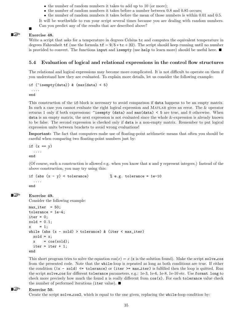
• the number of random numbers it takes to add up to 10 (or more);• the number of random numbers it takes before a number between 0.8 and 0.85 occurs;• the number of random numbers it takes before the mean of those numbers is within 0.01 and 0.5.

It will be worthwhile to run your script several times because you are dealing with random numbers.Can you predict any of the results that are described above?

�

Exercise 48.Write a script that asks for a temperature in degrees Celsius tc and computes the equivalent temperature indegrees Fahrenheit tf (use the formula tf = 9/5 ∗ tc + 32). The script should keep running until no numberis provided to convert. The functions input and isempty (use help to learn more) should be useful here. �

5.4 Evaluation of logical and relational expressions in the control flow structures

The relational and logical expressions may become more complicated. It is not difficult to operate on them ifyou understand how they are evaluated. To explain more details, let us consider the following example:

if (~isempty(data)) & (max(data) < 5)

....

end

This construction of the if-block is necessary to avoid comparison if data happens to be an empty matrix.In such a case you cannot evaluate the right logical expression and Matlab gives an error. The & operatorreturns 1 only if both expressions: ~isempty (data) and max(data) < 5 are true, and 0 otherwise. Whendata is an empty matrix, the next expression is not evaluated since the whole &-expression is already knownto be false. The second expression is checked only if data is a non-empty matrix. Remember to put logicalexpression units between brackets to avoid wrong evaluations!

Important: The fact that computers make use of floating-point arithmetic means that often you should becareful when comparing two floating-point numbers just by:

if (x == y)

....

end

(Of course, such a construction is allowed e.g. when you know that x and y represent integers.) Instead of theabove construction, you may try using this:

if (abs (x - y) < tolerance) % e.g. tolerance = 1e-10

....

end

Exercise 49.Consider the following example:

max_iter = 50;

tolerance = 1e-4;

iter = 0;

xold = 0.1;

x = 1;

while (abs (x - xold) > tolerance) & (iter < max_iter)

xold = x;

x = cos(xold);

iter = iter + 1;

end

This short program tries to solve the equation cos(x) = x (x is the solution found). Make the script solve cos

from the presented code. Note that the while-loop is repeated as long as both conditions are true. If eitherthe condition (|x - xold| <= tolerance) or (iter >= max iter) is fulfilled then the loop is quitted. Runthe script solve cos for different tolerance parameters, e.g.: 1e-3, 1e-6, 1e-8, 1e-10 etc. Use format long tocheck more precisely how much the found x is really different from cos(x). For each tolerance value checkthe number of performed iterations (iter value). �

Exercise 50.Create the script solve cos2, which is equal to the one given, replacing the while-loop condition by:

35

while (abs (x - xold) > tolerance) | (iter < max_iter)

Try to understand the difference and confirm your expectations by running solve cos2. What happens toiter? �

6 Numerical analysis

Numerical analysis can be used whenever it is impossible or very difficult to determine the analytical solution.Matlab can be used to find, for example, the minimum, maximum or integral of a certain function.

There are two ways to describe data with an analytical function:

• curve fitting or regression; finding a smooth curve that best fits (approximates) the data accordingto a criterion (e.g. best least square fit). The curve does not have to go through any of the data points.

• interpolation; the data are assumed to be correct, desired in a way to describe what happens betweenthe data points. In other words, given a finite set of points, the goal of interpolation is to find a functionfrom a given class of functions (e.g. polynomials) which passes through the specified points.

The figure below illustrates the difference between regression (curve fitting) and interpolation:

−5 0 5−8

−6

−4

−2

0

2

4

6

8

10interpolationfitting a 3D polynomial

In this section we will briefly discuss some issues on curve fitting, interpolation, function evaluation, integrationand differentiation. It is also possible to solve differential equations which are shortly treated in ”The Student

179-182 Edition of Matlab”book.

6.1 Curve fitting

Matlab interprets the best fit of a curve by the ‘least squares curve fitting’. The curve used is restricted153-156 to polynomials. With the command polyfit any polynomial can be fitted to the data. polyfit (x, y, n)

finds the coefficients of a polynomial of degree n that fits the data (finds the linear relation between x and y).Let’s start with finding a linear regression of some data:

>> x = 0:10;

>> y = [-.10 .24 1.02 1.58 2.84 2.76 2.99 4.05 4.83 5.22 7.51]

>> p = polyfit (x, y, 1) % find the fitting polynomial of order 1

p = 0.6772 -0.3914

The output of polyfit is a row vector of the polynomial coefficients, the solution of this example is thereforey = 0.6772x− 0.3914.

Exercise 51.Execute the above example. Plot the data and the fitted curve in a figure. Determine the 2nd and 9th orderpolynomial of these data as well, and display the solution in a figure.Hint : x1 = linspace(xmin,xmax,n); results in a vector with n element evenly distributed from xmin tillxmax. z = polyval(p,x1); calculates the values of the polynomial for every element of x1. �

Exercise 52.Define x and y as follows:

36

>> x = -5:5;

>> y = 0.2*x.^3 - x + 2; % a 3rd order polynomial

>> y = y + randn(11,1); % add some noise to y

Determine the 3rd order polynomial fitting y (note that because of added noise the coefficients are differentthat originally chosen). Try some other polynomials as well. Plot the results in a figure. �

6.2 Interpolation

The simplest way to examine an interpolation is by displaying the function plots with the command plot.157-161 The neighboring data points are connected with straight lines. This is called a linear interpolation. When

more data-points are taken into account the effect of interpolation becomes less visible. Analyze:

>> x1 = linspace(0,2*pi,2);

>> x2 = linspace(0,2*pi,4);

>> x3 = linspace(0,2*pi,16);

>> x4 = linspace(0,2*pi,256);

>> plot(x1,sin(x1),x2,sin(x2),x3,sin(x3),x4,sin(x4))

>> legend(’2 points’,’4 points’,’16 points’,’256 points’)

There exist also Matlab functions which interpolate between points, e.g. interp1 or spline, as a 1D157-165 interpolation and interp2, as a 2D interpolation. Perform the following commands:

>> N = 50;

>> x = linspace(0,5,N);

>> y = sin(x) .*sin(6*x);

>> subplot(2,1,1); plot(x,y);

>> hold on

>> p = randperm(N);

>> pp = p(1:round(N/2)); % choose randomly N/2 indices of points from [0,5]

>> pp = sort(pp); % sort the indices

>> xx = x(pp); % select the points

>> yy = y(pp);

>> plot(xx,yy,’ro-’) % this is a ’coarse’ version

>> yn = interp1(xx,yy,x,’nearest’); % nearest neighbor interpolation on all x points

>> plot(x,yn,’g’)

>> axis tight

>> legend(’Original’,’Crude version’,’Nearest neighbor interpolation’)

>>

>> subplot(2,1,2); plot(xx,yy,’ro-’);

>> hold on

>> yc = interp1(xx,yy,x,’linear’); % linear interpolation on all x points

>> plot(x,yc,’g’)

>> ys = spline(xx,yy,x); % spline interpolation

>> plot(x,ys,’k’)

>> axis tight

>> legend(’Crude version’,’Linear interpolation’,’Spline interpolation’)

You can also see a coarse approximation of the function peaks:

>> [X,Y,Z] = peaks(10);

>> [Xi,Yi] = meshgrid(-3:.25:3,-3:.25:3);

>> Zi = interp2(X,Y,Z,Xi,Yi);

>> mesh(Xi,Yi,Zi);

6.3 Evaluation of a function

As said before, the command plot plots a function by connecting defined data points. When a function is168-173 constant and not very interesting over some range and then acts unexpectedly wildly over another, it might

be misinterpreted by using plot. The command fplot is then more useful. An example is:

37

Command Result

fplot(’f’,[min x max x]) plots the function f on [min x, max x]fmin(’f’,min x,max x) returns the x-value for which the function f reaches minimum on [min x, max x]fzero(’f’,x0) returns the x-value for which the function f is zero in the neighborhood of x0

Table 8: Evaluation of a function.

>> x = 0:pi/8:2*pi;

>> y = sin(8*x);

>> plot(x,y,’b’)

>> hold on

>> fplot(’sin(8*z)’,[0 2*pi],’r’)

>> title(’sin(8*z)’)

>> hold off

Execution of these commands results in a figure with an almost straight blue line and a red sine. fplot canalso be used to plot a defined function:

>> f = ’sin(8*z)’;

>> fplot(f,[0 2*pi],’r’)

>> title(f)

6.3.1 Inline functions

It might be useful to define a function that will be only used during the current Matlab session. Matlab

offers a command inline to define the so-called inline functions in the Command Window, e.g.:

>> f = inline(’cos(x).*sin(2*x)’)

f =

Inline function:

f(x) = cos(x).*sin(2*x)

>> g = inline(’sqrt(x.^2+y.^2)’,’x’,’y’)

g =

Inline function:

g(x,y) = sqrt(x.^2+y.^2)

You can evaluate this function in a usual way:

>> f(-2)

ans =

-0.3149

>> g(3,4)

ans =

5

>> A = [1 2; 3 4];

>> B = [2 3; 4 5];

>> g(A,B) % the function also works with arrays

ans =

2.2361 3.6056

5.0000 6.4031

Let f(x) = 1(x−0.1)2+0.1 + 1

(x−1)2+0.1 . The point at which f takes its minimum is found using fmin (or fminbnd

in Matlab version 6.0). By default, the relative error is of 1e-4. It is possible, however, to obtain a higheraccuracy, by specifying an extra parameter while calling fmin.

>> format long % you need this format to see the change in accuracy

>> f = inline (’1./((x-0.1).^2 + 0.1) + 1./((x-1).^2 + 0.1)’);

>> fplot(f,[0 2]);

>> xm1 = fmin(f,0.3,1); fm1 = f(xm1);

>> xm2 = fmin(f,0.3,1,[0,1e-8]); fm2 = f(xm2);

>> [xm1, xm2] % compare the two answers

38

Important: Note that format does not change the accuracy of the numbers or calculations; it just changesthe numbers of digits displayed on the screen.

Exercise 53.Use fmin (fminbnd when applicable) to find the maximum of f(x) = 1

(x−0.1)2+0.1 + 1(x−1)2+0.1 in the interval

[0, 0.5]. Choose an error tolerance such that the maximum is correct to ±10−6. If xm denotes the computedsolution, check the answer by evaluating f at xm +10−6 and xm− 10−6. The values should be smaller at boththese neighboring points. Hint: there is no function fmax. Find the minimum of −f(x), instead. �

Exercise 54.Determine the maximum of the function f(x) = x cos(x) over the interval 10 < x < 15. �

Exercise 55.Find the zero, i.e x0, of the functions f(x) = cos(x) and g(x) = sin(2x) around the point 2. Use a commandfrom Table 8. Check that the values are approximately zero for x0 and the signs of f at x0 ± 10−4. �

6.4 Integration and differentiation

The integral, or the surface underneath a 2D function, can be determined with the command trapz. trapz

173-182 does this by measuring the surface between the x-axis and the data points, connected by the straight lines.The accuracy of this method depends on the distance between the data points:

>> x = 0:0.5:10; y = 0.5 * sqrt(x) + x .* sin(x);

>> integral1 = trapz(x,y)

integral1 =

18.1655

>> x = 0:0.05:10; y = 0.5 * sqrt(x) + x .* sin(x);

>> integral2 = trapz(x,y)

integral2 =

18.3846

A more accurate result can be obtained by using the command quad or quadl, which also numerically evaluatean integral of the function f specified by a string or by an inline definition. Let f = 1

(x−0.1)2+0.1 + 1(x−1)2+0.1 .

>> f = ’1./((x-0.1).^2 + 0.1) + 1./((x-1).^2 + 0.1)’;

>> integral1 = quad(f,0,2)

>> integral2 = quadl(f,0,2)

You can also add an extra parameter to quad and quadl, specifying the accuracy.

Exercise 56.Find the integral of the function f(x) = e−x2/2 over the interval [−3, 3]. Exercise with different Matlab

commands and different accuracy. �

Differentiation is done by determining the slope in each data point. Numerically this is done by first fitting apolynomial, followed by differentiating this function:

>> x = 0:10;

>> y = [-.10 .24 1.02 -1.58 2.84 2.76 7.75 .35 4.83 5.22 7.51];

>> p = polyfit(x,y,5)

p =

0.0026 -0.0554 0.3634 -0.6888 0.2747 0.0877

>> dp = polyder(p)

dp =

0.0132 -0.2216 1.0903 -1.3776 0.2747

>> x1 = linspace(0,10,200);

>> z = polyval(p,x1);

>> dz = polyval(dp,x1);

>> plot(x,y,’g.-’,x1,z,’b’,x1,dz,’r:’)

>> legend(’data points’,’curve fit’,’derivative’)

Exercise 57.Determine the integral and derivative of the 4th polynomial fitted through (x,y) with x = 4:13 and y =

[12.84 12.00 7.24 -0.96 -11.16 -20.96 -27.00 -24.96 -9.56 25.44]. �

39

6.5 Numerical computations and the control flow structures

Take a look at the problem of a Taylor expansion. The series will be determined numerically until the additionalterms are smaller than a defined precision. Look at the Taylor expansion of 1

1−x = 1+x+x2+. . . with x = 0.42:

s = 0; x = 1; s = 0; x = 1;

x0 = 0.42; x0 = 0.42;

while (x > 1e-6) or while (x > (1e-6)*s)

s = s + x; s = s + x;

x = x * x0; x = x * x0;

end end

The approximation of 11−x is returned in s (from sum). In the first case (on the left), the iteration process is

stopped as soon as the next term t is smaller than an absolute value of 1e-6. In the other case, this value isrelative to the outcome.

Exercise 58.Find the Taylor expansion of 1

1−x and sin(x) = x− x3

3! + x5

5! − . . . with the absolute precision of 1e-5 for x = 0.4and x = −0.4. �

It is also possible to determine the Taylor expansion of 11−x = 1 + x + x2 + . . . with 30 terms (x = 0.42):

s = 1; x = 1; s = 1; x = 1; x0 = 0.42;

x0 = 0.42; n1 = 1; n2 = 30;

n = 30; step = 1;

for k = 1:n for k = n1:step:n2

x = x * x0; or x = x * x0;

s = s + x; s = s + x;

end end

showing that the index k can be indicated with a starting point, step size and end point.

7 Script and function m-files

7.1 Script m-files

Matlab commands can be entered at the Matlab prompt. When a problem is more complicated this becomes29-33 inefficient. A solution is using script m-files . They are useful when the number of commands increases or when

you want to change values of some variables and re-evaluate them quickly. Formally, a script is an external filethat contains a sequence of Matlab commands (statements). However, it is not a function, since there areno input/output parameters and the script variables remain in the workspace. So, when you run a script,the commands in it are executed as if they have been entered through the keyboard.

Exercise 59.Create yourself a script: open the Matlab editor (go to the File menu-bar, choose the Open option andthen m-file; the Matlab Editor Window will appear), enter the lines listed below and save as sinplot.m:

x = 0:0.2:6;

y = sin(x);

plot(x,y);

title(’Plot of y = sin(x)’);

and then run it by:

>> sinplot

The sinplot script affects the workspace. Check:

>> clear % all variables are removed from the workspace

>> who % no variables present

>> sinplot

>> who

Your variables are:

40

x y

�

These generic names, x and y, may be easily used in further computations and this can cause side effects . Sideeffects occur in general when a set of commands change variables other than the input arguments. Since scriptscreate and change variables in the workspace (without warning), a bug, hard to track down, may easily appear.So, it is important to remember that the commands within a script have access to all variables in theworkspace and all variables created in this script become a part of the workspace. Therefore, itis better to use function m-files (see section 7.2), when there is a specific problem to be solved.

Exercise 60.Create a script which:

1. plots the function y = 2cos(x) at the range [−10, 10]. Choose a sufficient length for x in order to obtaina smooth plot.

2. plots the functions y = x2 and x = y2 in the same figure. Add a title, legend and axes descriptions.�

optional

The diary command can be also useful when creating scripts. diary on begins saving the text that is enteredand displayed in the Command Window into a file called diary . Another name can be used alternatively, whenit is provided instead of on and after the diary. diary off stops the saving procedure.

Exercise 61.Check yourself the following:

>> diary myplot.m

>> x = 0:0.2:6;

>> y = sin(x);

>> z = x * y;

??? Error using ==> *

Inner matrix dimensions must agree.

>> z = x .* y; % correction

>> plot(x,z);

>> title(’Plot of y = x * sin(x)’);

>> diary off

Note, that before running myplot, its contents must be edited by removing the >> signs and the error note. �

end optional

Exercise 62.Write the script cubic roots that for given a, b and c returns the roots of the cubic equation: a x2+b x+c = 0.�

Exercise 63.Write a script that plots the graph of equilateral triangle with two vertices [a, a] and [b, a]. Find the thirdvertex. Use fill to paint the triangle. �

7.2 Function m-file

Functions m-files are true subprograms, since they take input arguments and/or return output parameters.126-134 They can call other functions, as well. Variables defined and used inside a function, different from the in-

put/output arguments, are invisible to other functions and the command environment. The general syntax ofa function is presented below:

function [outputArgs] = function_name (inputArgs)

outputArgs are enclosed in [ ]:

– a comma-separated list of variable names;

– [ ] is optional when only one argument is present;

– functions without outputArgs are legal4.

4in other programming languages, functions without output arguments are called procedures

41

inputArgs are enclosed in ( ):

– a comma-separated list of variable names;

– functions without inputArgs are legal.

Matlab provides a structure for creating your own functions. The first line of the file should be a definition ofa new function (also called a header). After that, a continuous sequence of comment lines should appear. Theirgoal is to explain what the function does, especially when this is not trivial. Not only a general description,but also the expected input parameters, returned output parameters and synopsis should appear there. Thecomment lines (counted up to the first non-comment line) are important since they are displayed in responseto the help command. Finally, the remainder of the function is called the body. Function m-files terminateexecution and return when they reached the end of the file or, alternatively, when the command return isencountered. As an example, the function average is defined as follows:

input argumentthe first line must bethe function definition

help average

a blank line within the comment;Notes information will NOT appearwhen you ask:

%AVERAGE computes the average value of a vector x

function avr = average (x)

function nameoutput argument

comment % and returns it in avr

% Notes: an example of a function

n = length(x);avr = sum(x)/n;return;

function body

Important: The name of the function and the name of the file stored on disk should be identical . In ourcase, the function should be stored in a file called average.m.

Exercise 64.Create the function average and store it on disk as average.m. Remember about the comment lines. Checkits usability by calling help average. Run average.m by typing avr1 = average(1:10); �

Here is an another example of a function:

function [avr,sd] = stat(x)

%STAT Simple statistics.

% Computes the average value and the standard deviation of a vector x.

n = length(x);

avr = sum(x)/n;

sd = sqrt(sum((x - avr).^2)/n);

return;

Warning: The functions mean and std already exist in Matlab. As long as a function name is used asvariable name, Matlab can not perform the function. Many other, easily appealing names, such as sum orprod are reserved by Matlab functions, so be careful when choosing your names (see section 12.3).

The return statement can be used to force an early return. An exemplary use of the return is given below:

function d = determinant(A)

%DETERMINANT Computes the determinant of a matrix A

[m,n] = size(A);

if (m ~= n)

disp (’Error. Matrix should be square.’);

return;

else

d = det(A); % standard Matlab function

end

return;

Analyze the use of the return command in the function checkarg, which is presented in section 7.2.1 as well.

When controlling the proper use of parameters, the function error may become useful. It displays an error129 message, aborts function execution, and returns to the command environment. Here is an example:

if (a >= 1)

42

error (’a must be smaller than 1’);

end

Change some scripts that you created into functions, e.g. create the function drag, computing the dragcoefficient (see section 5.2), or solve cos (see section 5.4) or cubic roots (see section 7.1).

Exercise 65.Write the function [elems, mns] = nonzero(A) that takes as the input argument a matrix A and returns allnonzero elements of A in the column vector elems. The output parameter mns holds values of the means of allcolumns of A. �

Exercise 66.Create the function [A,B,C] = sides(a,b,c) that takes three positive numbers a, b and c. If they are sidesof a triangle, then the function returns its angles A, B and C, measured in degrees. Display an error whennecessary. �

Exercise 67.The area of a triangle with sides of length a, b, and c is given by: ar =

√

s (s− a) (s− b) (s− c), wheres = (a + b + c)/2. Write a function that accepts a, b and c as inputs and returns the value ar as output.Note that the sides should be non-negative and should fulfill the triangle inequality. Make use of the error

command. �

Exercise 68.Create the function randint that randomly generates a matrix of integer numbers (use the command rand).These integers should come from the interval [a, b]. Exercise in documenting the function. Use the followingfunction header:

function r = randint(m,n,a,b) % a m-by-n matrix

If this seems too difficult, start first with the fixed interval, e.g. [a, b] = [0, 5] (and remove a and b from thefunction definition) and then try to make it work for an arbitrary interval. �

optional

A function m-file may contain more than one function. The function appearing first in the m-file sharesthe file name, as mentioned before. Other functions are subfunctions and can be called from the primaryfunction only. So, they cannot be accessed from outside the file, in which they are defined (neither fromthe Command Window nor via other m-files). A subfunction is created by defining a new function with thefunction statement after the body of the preceding function. The use of subfunctions is recommended tokeep the function readable when it becomes too long and too complicated. For example, average is now asubfunction within the file stat.m:

function [a,sd] = stat(x)

%STAT Simple statistics.

% Computes the average value and the standard deviation of a vector x.

n = length(x);

a = average(x,n);

sd = sqrt(sum((x - avr).^2)/n);

return;

function a = average (x,n)

%AVERAGE subfunction

a = sum(x)/n;

return;

end optional

7.2.1 Special function variables

Each function has two internal variables: nargin - the number of function input arguments that were used tocall the function and nargout - the number of output arguments. Analyze the following function:

function [out1,out2] = checkarg (in1,in2,in3)

%CHECKARG Demo on using the nargin and nargout variables.

if (nargin == 0)

disp(’no input arguments’);

43

return;

elseif (nargin == 1)

s = in1;

p = in1;

disp(’1 input argument’);

elseif (nargin == 2)

s = in1+in2;

p = in1*in2;

disp(’2 input arguments’);

elseif (nargin == 3)

s = in1+in2+in3;

p = in1*in2*in3;

disp(’3 input arguments’);

else

error(’Too many inputs.’);

end

if (nargout == 0)

return;

elseif (nargout == 1)

out1 = s;

else

out1 = s;

out2 = p;

end

Exercise 69.Construct the function checkarg, call it with different number of input and output arguments and try tounderstand its behavior. For example:

>> checkarg

>> s = checkarg(-6)

>> s = checkarg(23,7)

>> [s,p] = checkarg(3,4,5)

�

7.2.2 Local and global variables

Each m-file function has access to a part of memory separate from Matlab ’s workspace. This is called thefunction workspace. This means that each m-file function has its own local variables, which are separate fromthose of other function and from the workspace. To understand it better analyze the following diagram:

Matlab workspace>> a = -1;

>> b = 20;

>> c = myfun (a,b)

(a, b) −→ (x, y)

c ←− z

myfun.mfunction z = myfun (x,y)

...

z = x + cos(x-y);

return;

In the Matlab workspace, variables a, b and c are available. Variables x, y and z are visible only in thefunction myfun. However, if several functions and/or the workspace, all declare a particular variable as global,then they all share this variable (see help global). Any assignment to that variable is available to all otherfunctions and/or the workspace. However, you should be careful when using global variables. It is very easyto get confused and end up with serious errors.

optional

7.2.3 Indirect function evaluation

Using indirect function evaluation makes programming even more general, since functions can become inputarguments. The crucial Matlab command here is feval, an abbreviation of function evaluation. The feval

command allows execution of a function specified by a string. The general definition is as follows:

44

[y1,..,yn] = feval (F,x1,...,xn),

where F is a name of a function defined in Matlab, x1,...,xn are input arguments and y1,...,yn arepossible output parameters. Consider an example:

>> x = pi; y = cos(x);

>> z = feval(’cos’,x);

The last command is also equivalent to the following two expressions:

>> F = ’cos’;

>> z = feval(F,x)

Indirect function evaluation is a nice tool to build a program with a function given as an argument.

Exercise 70.Create the function funplot and try to understand how it works:

function funplot (F, xstart, xend, col);

%FUNPLOT makes a plot of the function F at the interval [xstart, xend].

% The plot should be made in one of the standard Matlab colors, so

% ’col’ is one of the following value: ’b’,’k’,’m’,’g’,’w’,’y’ or ’r’.

% default values:

% [xstart,xend] = [0,10]

% col = ’b’

% Note: illustrates the use of feval command

if (nargin == 0)

error (’No function is provided.’);

end

if (nargin < 2)

xstart = 0;

xend = 10;

end

if (nargin == 2)

error (’Wrong number of arguments. You should provide xstart and xend.’);

end

if (nargin < 4)

col = ’b’;

end

if (xstart == xend),

error (’The [xstart, xend] should be a non-zero range.’);

elseif (xstart > xend),

exchange = xend;

xend = xstart;

xstart = exchange;

end

switch col

case {’b’,’k’,’m’,’g’,’w’,’y’,’r’}

; % do nothing; the right color choice

otherwise

error (’Wrong col value provided.’)

end

x = linspace(xstart, xend);

y = feval(F,x);

plot (x,y,col);

description = [’Plot of ’, F];

title (description);

return;

45

Note the use of comments, the nargin variable and the switch-construction. Call funplot for different built-in functions, like sin, exp, etc. Test it for your own functions as well. Write for example a function myfun thatcomputes sin(x cos(x)) or log( |x sin(x)| ). Explain why it would be wrong to use the fragment given belowinstead of its equivalent part in funplot.

if nargin < 2

xstart = 0;

xend = 10;

elseif nargin < 3

error (’Wrong number of arguments. You should provide xstart and xend.’);

elseif nargin < 4

col = ’b’;

end

�end optional

7.3 Scripts vs. functions

The most important difference between a script and a function is that all script’s parameters and variablesare externally accessible (i.e. in the workspace), where function variables are not. Therefore, a script is agood tool for documenting work, designing experiments and testing. In general, create a function to solve agiven problem for arbitrary parameters. Use a script to run functions for specific parameters required by theassignment.

Exercise 71.Create the function binom that computes the value of the binomial symbol

(

nk

)

. Make the function header:function b = binom (n,k). Note that in order to write this function, you will have to create the factorial

function, which computes the value of n! = 1 ∗ 2 ∗ ... ∗ n. This may become a separate function (enclosedin a new file) or a subfunction in the binom.m file. Try to implement both cases if you got acquainted withthe notion of a subfunction. Having created the binom function, write a script that displays on screen all thebinomial symbols for n = 8 and k = 1, 2, ..., 8 or write a script that displays on screen the following ’triangle’(use the fprintf command; try help fprintf or see section 8.2):

(

11

)

(

21

) (

22

)

(

31

) (

32

) (

33

)

(

41

) (

42

) (

43

) (

44

)

�

Exercise 72.Solve the following exercises by using either a script or a function. The nature of the input/output and displayoptions is left to you. Problems are presented with the increasing difficulty; start simple and add complexity.If possible, try to solve all of them.

1. Write a function which computes the cumulative product of a vector elements. The cumulative productup to xj - the j-th element of the vector x is defined by Cj =

∏jk=1 xk for j = 1 : length(x). Check

your results with the built-in function cumprod.

2. Write Matlab function m = wmean (x,w) computing the weighted arithmetic mean, given the vector x

and a vector of nonnegative weights w, such that∑n

i=1 wi > 0, i.e.∑

n

i=1wi xi

∑

n

i=1wi

. Add error messages to

terminate execution of the function in the case when:

– x and w are of different lengths,– at least one element of w s negative,– sum of all weights is equal to zero.

3. Compute the value of π using the following series:

π2 − 8

16=

∞∑

n=1

1

(2n− 1)2 (2n + 1)2

How many terms are needed to obtain an accuracy of 1e-12? How accurate is the sum of 100 terms?

46

4. Write a program that approximates π by computing the sum:

π

4≈

m∑

n=0

(−1)n

2n + 1

The more terms in summation the larger the accuracy (although this is not an efficient formula, sinceyou add and subtract numbers). How many terms are needed to approximate π with 5 decimals? Usethe sum to approximate π using 10, 100, 1e3, 1e4, 5e4, 1e5, 5e5 and 1e6 terms. For each of these numberscompute the approximation error. Plot the error as a function of the term numbers used in a summation.

5. The Fibonacci numbers are computed according to the following relation:

Fn = Fn−1 + Fn−2, with F0 = F1 = 1

– Compute the first 10 Fibonacci numbers.– For the first 50 Fibonacci numbers, compute the ratio Fn

Fn−1. It is claimed that this ratio approaches

the value of the golden mean 1+√

52 . What do your results show?

6. Consider a problem of computing the n-th Fibonacci number. Find three different ways to implementthis and construct three different functions, say fib1, fib2 and fib3. Measure the execution time ofeach function (use the commands tic and toc) for, say, n = 20, 40 or 100.

7. The Legendre polynomials Pn(x) are defined by the following recurrence relation:

(n + 1) Pn+1(x)− (2n + 1) x Pn(x) + n Pn−1(x) = 0

with P0(x) = 1, P1(x) = x and P2(x) = (3x2 − 1)/2. Compute the next 3 Legendre polynomials andplot all 6 over the interval [−1, 1].

8. Write a script that asks for an integer n (or a function that has n as the input argument) and thencomputes the following: while the value of n is greater than 1, replace the integer with (n/2) if theinteger is even. Otherwise, replace the integer with (3n + 1). Make provision to count the number ofvalues in (or the length of) the sequence that results.

Example calculation: If n = 10, the sequence of integers is 5, 16, 8, 4, 2, 1, so the length is 6.

Make a plot of the length of the sequence that occurs as a function of the integers from 2 to 30. Forexample, when n = 10, the length is 6 while for n = 15, the length is 17. Is there any pattern? Try largernumbers to see if any pattern occurs. Is there any integer for which the sequence does not terminate?

9. Provide all prime numbers smaller then the given N .�

8 Text

8.1 Character strings

Although Matlab mainly works with numbers, it might occasionally be necessary to operate on text. Text94-99 is saved as a character string. The string is a vector of ASCII values which are displayed as their character

string representation. Since text is a vector of characters, it can be addressed in the same way as any vector.An example:

>> t = ’This is a character string’

t =

This is a character string

>> size(t)

ans =

1 27

>> whos

Name Size Bytes Class

t 1x27 54 char array

>> t(10:19)

ans =

47

character

>> t([2,3,10,17])

ans =

hi t

To see the underlying ASCII representation, the string has to be converted using the command double or abs:

>> double(t(1:12))

ans =

84 104 105 115 32 105 115 32 97 32 99 104

The function char provides the reverse transformation:

>> t([16:17])

ans =

ct

>> t([16:17])+3 % to perform a mathematical operation ASCII codes are used

ans =

102 119

>> t([16:17])-3 % ASCII codes again

ans =

96 113

>> char(t([16:17])-2) % transform ASCII codes to characters

ans =

ar

Exercise 73.Perform the described commands. Use string t to form a new string u that contains the word ”character”only. Convert string u to form the same word spelled backwards, i.e. u1 = retcarahc. �

The tables on page 97 and 98 of ”The Student Edition of Matlab” book give an overview of string conversionsand functions. With e.g. findstr, a string can be searched for a character or a combination of characters.Some examples on the use of different string functions are given below:

>> findstr(t, ’c’) % finds a character ’c’ in string t; positions are returned

ans =

11 16

>> findstr(t, ’racter’) % finds the beginning of a string ’racter’ in t

ans =

14

>> findstr(t,u) % finds string u in string t; returns the position

ans =

11

>> strcat(u,u1) % concatenates multiple strings: u and u1

ans =

characterretcarahc

>> strcmp(u,u1) % comparison of two strings;

ans = % 1 for identical strings; 0 for different strings

0

>> q = num2str(34.35) % converts a number into a string

q =

34.35

>> z = str2num(’7.6’) % converts a string into a number

z =

7.6

>> whos q z % q is now a string, i.e. a character array; z is a number

Name Size Bytes Class

q 1x5 10 char array

z 1x1 8 double array

>> t = str2num(’1 -7 2’) % converts a string into a vector of number

t =

48

1 -7 2

>> t = str2num(’1 - 7 2’) % here spaces around the sign - or + are important!

t = % performs: [1-7, 2]

-6 2

>> A = round(4*rand(3,3))+0.5;

>> ss = num2str(A) % since A is random, you will get different numbers here

ss =

-3.5 -3.5 6.5

-2.5 -1.5 0.5

5.5 -1.5 -3.5

>> whos ss

Name Size Bytes Class

ss 3x28 168 char array

>> ss(2,1), ss(3,15:28) % ss is a char array; you can address it in a standard way

ans =

-

ans =

.5 -3.5

>> ss(1:2,1:3)

ans =

-3.

-2.

Exercise 74.Perform the commands shown in the example above. Define another string, e.g. s = ’Nothing wastes more

energy than worrying’ and exercise with findstr. �

Exercise 75.Become familiar with the commands: num2str and str2num. Check e.g. what happens with ss = num2str([1

2 3; 4 5 6]) or q = str2num(’1 3.25; 5 5.5’). Analyze also the commands str2double and int2str

(use help to get more information). �

8.2 Text input and output

The input command can be used to prompt (ask) the user for numeric or string input:31-33

>> myname = input(’Enter your name: ’,’s’);

>> age = input(’Enter your age: ’);

You have learned in section 7.2 that inputs can be passed on to functions. This is a recommended approach,since using the input command for more complex programs makes automatic computation impossible.

There are two common text output functions: disp and fprintf. The disp function only displays the valueof one parameter, either a numerical array or a string (the recognition is done automatically). For example:

>> disp(’This is a statement.’) % a string

This is a statement.

>> disp(rand(3)) % a matrix

0.2221 0.0129 0.8519

0.4885 0.0538 0.5039

0.2290 0.3949 0.4239

The fprintf function (familiar to C programmers) is useful for writing data to a file (see section 11.1) or97 printing on screen when precise formatting is important. Try, for instance (an explanation will follow):

>> x = 2;

>> fprintf(’Square root of %g is %8.6f.\n’, x, sqrt(x));

Square root of 2 is 1.414214.

>> str = ’beginning’;

>> fprintf(’Every %s is difficult.\n’,str);

Every beginning is difficult.

Formally, fprintf converts, formats and prints its arguments to a file or displays them on screen accordingto a format specification. For displaying on screen, the following syntax is used:

49

fprintf (format,a,...)

The format string contains ordinary characters, which are copied to the output, and conversion specifications ,each of which converts and prints the next successive argument to fprintf. Each conversion specification isintroduced by the character ’%’ and ended by a conversion character. Between the ’%’ and the conversioncharacter there may appear:

• a minus sign; controlling the alignment within the field defined.

• a digit string specifying a minimum field length; The converted number will be printed in a field at leastthis wide, and wider if necessary.

• a period which separates the field width from the next digit string;

• a digit string - the precision which specifies the maximum number of characters to be printed from astring or the number of digits printed after decimal point of a single or double type.

Format specification is given below in terms of the conversion characters and their meanings:

The argumentd is converted into decimal notation;u is converted into unsigned decimal notation;c is taken to be a single character;s is a string;e is taken to be a single or double and converted into decimal notation of

the form: [-]m.nnnnnnE[±]xx, where the length of n’s is specified by the precision;f is taken to be a single or double and converted into decimal notation of

the form:[-]mmm.nnnnn, where the length of n’s is specified by the precision;g is specified by e or f, whichever is shorter; non-significant zeros are not printed;

The special formats \n, \r, \t, \b can be used to produce next line (i.e. makes sure that the next commandor output will be written on the next line), carriage return, tab, and backspace respectively. Use \\ to producea backslash character and %% to produce the percent character.

Analyze the following example:

>> fprintf(’look at %20.6e!\n’, 1000*sqrt(2))

look at 1.414214e+3!

>> fprintf(’look at %-20.6f!’, 1000*sqrt(2))

look at 1414.213562 ! >>

For both commands, the minimum field length is 20 and the number of digits after the decimal point is 6.In the first case, the value of 1000*sqrt(2) is padded on the right, in the second case, because of the ’-’, itappears on the left. The difference in the presentation is caused by the conversion characters e and f .

Exercise 76.Try to exercise to understand how to use the input, disp and fprintf commands. For instance, try to reada vector with real numbers using input. Then, try to display this vector, both by calling disp and formattingan output by fprintf. Make a few variations. Try the same with a string. �

Exercise 77.Study the following examples in order to become familiar with the fprintf possibilities and exercise yourselfto understand how to use these specifications:

>> str = ’life is beautiful’;

>> fprintf(’My sentence is: %s\n’,str); % note the \n format

My sentence is: life is beautiful

>> fprintf(’My sentence is: %30s\n’,str);

My sentence is: life is beautiful

>> fprintf(’My sentence is: %30.10s\n’,str);

My sentence is: life is be

>> fprintf(’My sentence is: %-20.10s\n’,str);

My sentence is: life is be

>>

>> name = ’John’;

>> age = 30;

50

>> salary = 6130.50;

>> fprintf(’My name is %4s. I am %2d. My salary is f %7.2f.\n’,name, age, salary);

>> My name is John. I am 30. My salary is f 6130.50.

>>

>> x = [0, 0.5, 1];

>> y = [x; exp(x)];

>> fprintf(’%6.2f %12.8f\n’,y);

0.00 1.00000000

0.50 1.64872127

1.00 2.71828183

>>

>> fprintf(’%6.1e %12.4e\n’,y);

0.0e+00 1.0000e+00

5.0e-01 1.6487e+00

1.0e+00 2.7183e+00

>>

>> x = 1:3:7;

>> y = [x; sin(x)];

>> fprintf(’%2d %10.4g\n’,y);

1 0.8415

4 -0.7568

7 0.657

�

Warning: fprintf uses its first argument to decide how many arguments follow and what their types are.If you provide a wrong type or there are not enough arguments, you will get nonsense for an answers. So, becareful with formatting your output. Look, e.g., what happens in the following case (age is not provided):

>> fprintf(’My name is %4s. I am %2d. My salary is f %7.2f.\n’,name,salary);

My name is John. I am 6.130500e+03. My salary is f >>

Remark: The function sprintf is related to fprintf, but writes to a string instead. Analyze the example:

>> str = sprintf(’My name is %4s. I am %2d. My salary is f %7.2f.\n’,name,age,salary)

str =

My name is John. I am 30. My salary is f 6500.50.

Exercise 78.Define a string s = ’How much wood could a wood-chuck chuck if a wood-chuck could chuck wood?’.Exercise with findstr, i.e. find all appearances of the substrings ’wood’, ’o’, ’uc’ or ’could’. Try to buildss by concatenation of separate words. Try to do this in a few ways, e.g. make use of strcat, disp, sprintfor fprintf. �

Exercise 79.• Write a script/function that converts a Roman numeral to its decimal equivalent. There are two distinct

situations. The ’old’ style where the order of the symbols does not matter. In this case, IX and XI bothmean 10 + 1 or 11. You should be able to handle the following conversion table:

Roman Decimal

I 1

V 5

X 10

L 50

C 100

D 500

M 1000

The ’new’ style where the order of the symbols does matter. For example, IX is 9 (10 - 1), XC is 90(100 - 10). The conversion table given above still holds and you may assume for this case that the onlyinstances of order you will encounter are: IV (4), IX (9), XL (40), XC (90), CD (400) and CM (900).The function input will be useful here. Hint: try the case of the ’old’ style first.

• Write a function that will do the inverse of the previous problem - convert a decimal number into aRoman number.�

51

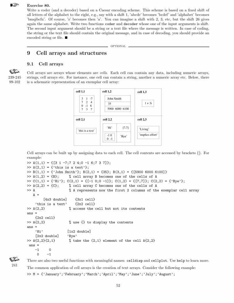
Exercise 80.Write a coder (and a decoder) based on a Caesar encoding scheme. This scheme is based on a fixed shift ofall letters of the alphabet to the right, e.g., say with a shift 1, ’abcde’ becomes ’bcdef’ and ’alphabet’ becomes’bmqibcfu’. Of course, ’z’ becomes then ’a’. You can imagine a shift with 2, 3, etc, but the shift 26 givesagain the same alphabet. Write two functions coder and decoder whose one of the input arguments is shift.The second input argument should be a string or a text file where the message is written. In case of coding,the string or the text file should contain the original message, and in case of decoding, you should provide anencoded string or file. �

optional

9 Cell arrays and structures

9.1 Cell arrays

Cell arrays are arrays whose elements are cells. Each cell can contain any data, including numeric arrays,239-24599-102

strings, cell arrays etc. For instance, one cell can contain a string, another a numeric array etc. Below, thereis a schematic representation of an exemplar cell array:

’this is a text’-1 00 -1

35

5900 6000 6100

John Smith

’implies effort’

’Living’

1 + 3i

cell 2,2

’Bye’

’Hi’ [7,7]

3 1 -77 2 40 -1 67 3 7

cell 1,1 cell 1,2 cell 1,3

cell 2,3cell 2,1

Cell arrays can be built up by assigning data to each cell. The cell contents are accessed by brackets {}. Forexample:

>> A(1,1) = {[3 1 -7;7 2 4;0 -1 6;7 3 7]};

>> A(2,1) = {’this is a text’};

>> B(1,1) = {’John Smith’}; B(2,1) = {35}; B(3,1) = {[5900 6000 6100]}

>> A(1,2) = {B}; % cell array B becomes one of the cells of A

>> C(1,1) = {’Hi’}; C(2,1) = {[-1 0;0 -1]}; C(1,2) = {[7,7]}; C(2,2) = {’Bye’};

>> A(2,2) = {C}; % cell array C becomes one of the cells of A

>> A % A represents now the first 2 columns of the exemplar cell array

A =

[4x3 double] {3x1 cell}

’this is a text’ {2x2 cell}

>> A(2,2) % access the cell but not its contents

ans =

{2x2 cell}

>> A{2,2} % use {} to display the contents

ans =

’Hi’ [1x2 double]

[2x2 double] ’Bye’

>> A{2,2}{2,1} % take the (2,1) element of the cell A{2,2}

ans =

-1 0

0 -1

There are also two useful functions with meaningful names: celldisp and cellplot. Use help to learn more.241

The common application of cell arrays is the creation of text arrays. Consider the following example:

>> M = {’January’;’February’;’March’;’April’;’May’;’June’;’July’;’August’;

52

’September’;’October’;’November’;’December’};

>> fprintf (’It is %s.\n’, M{9});

It is September.

Exercise 81.Exercise with the concept of a cell array, first by typing the examples presented above. Next, create a cellarray W with the names of week days, and using the command fprintf, display on screen the current datewith the day of the week. The goal of this exercise is also to use fprintf with a format for a day name and adate, in the spirit of the above example. �

9.2 Structures

Structures are Matlab arrays with data objects composed of fields. Each field contains one item of informa-245-249 tion. For example, one field might include a string representing a name, another a scalar representing age or

an array of the last few salaries. Structures are especially useful for creating and handling a database. Oneof the possible ways to create a structure is by assigning data to individual fields. Imagine that you want toconstruct a database with some information on workers of a company:

>> worker.name = ’John Smith’;

>> worker.age = 35;

>> worker.salary = [5900, 6000, 6100];

>> worker =

name: ’John Smith’

age: 35

salary: [5900 6000 6100]

In this way, a 1× 1 structure array worker with three fields: name, age and salary is constructed. To expandthe structure, add a subscript after the structure name:

>> worker(2).name = ’Linda Murphy’; % after this, a 2nd subarray is created

>> worker(2).age = 41;

>> worker(2).salary = [7301, 7301]; % field sizes do not need to match!

>> worker

1x2 struct array with fields:

name

age

salary

Since the structure has now size 1 × 2, Matlab does not display contents of all fields. The data is noworganized as follows:

worker array

worker(1)

.name John Smith

.age 35

.salary 5900, 6000, 6100

worker(2)

.name Linda Murphy

.age 41

.salary 7301, 7301

Structures can also be build by using the struct function, for example:

>> employee=struct( ’name’,’John Smith’,’age’,35,’salary’,[5900, 6000, 6100]);

To access an entire field, include a field name after a period. To access a subarray, follow the standard way ofusing subscripts:

53

>> worker(1).age

35

>> worker(2).salary(2)

7301

>> worker(2)

name: ’Linda Murphy’

age: 41

salary: [7301 7301]

An alternative way is to use the getfield function:

>> getfield(worker,{2},’salary’)

7301 7301

There exist also the function setfield, which allows assigning values . New fields can be added or deleted248 from every structure. To delete a field, use the command rmfield. Analyze the following example:

>> worker2 = worker;

>> worker2 = rmfield (worker, ’age’);

>> worker2(2).street = ’Bakerstreet 5’;

>> worker2(2)

name: ’Linda Murphy’

salary: [7301 7301]

street: ’Bakerstreet 5’

>> worker2(1)

name: ’John Smith’

salary: [5900 6000 6100] % in all other substructures address field is empty

street: [] % you should assign new values for each substructure

Operating on fields and field elements is done in the same way as on any other array. Consider the followingexample, where the average salary for each worker is computed.

avr_salary(1) = mean (worker(1).salary);

avr_salary(2) = mean (worker(2).salary);

Remark: structures as a concept are common organizations of data in other programming languages. Theyare created in different ways, but the intention remains the same.

Exercise 82.Construct a structure friend, with the following fields: name, address, age, birthday. Insert a few friendswith related information. Remove e.g. the field age and add the field phone. �

General remark: Classes and objects allow for adding new data types and new operations to Matlab. Forinstance, the class of a variable describes the structure of the variables and the operations permitted as wellas functions to be used. An object is an instance of a particular classs. The use of classes and objects is thebase of object-oriented programming , which is also possible in Matlab.

end optional

10 Optimizing the performance of Matlab code

Matlab is a matrix language, so it is designed for matrix operations. For best performance you should takeadvantage of this fact.

10.1 Vectorization - speed-up of computations

Vectorization is simply the use of compact expressions that operate on all elements of a vector without explicitly43-62 executing a loop. Matlab is optimized such that vector or matrix operations are much more efficient than

loops. Most built-in functions support vectorized operations. So, try to replace loops with vector operations,when possible. For example, instead of using:

for i = 1:10

t(i) = 2*i;

y(i) = sin (t(i));

end

54

try this:

t = 2:2:20;

y = sin (t);

Copying or transforming matrices can be vectorized, as well. Check the equivalence between the scalar version:

n = 10;

A = rand(n,n);

B = ones(n,n);

for k=1:n

B(2,k) = A(2,k); % A and B have the same size

end

and the vectorized code of the last loop:

B(2,:) = A(2,:);

or between the following loop:

for k=1:n

B(k,1) = A(k,k);

end

and the vectorized expression:

B(1:n,1) = diag(A(1:n,1:n));

Logical operations and proper use of the colon notation make the programs work faster. However, someexperience is needed to do this correctly. Therefore, the advice is: start first with the scalar code andthen vectorize it where possible, by removing loops.

Exercise 83.Look at your script or function m-files already written, especially your loop exercises. Try to vectorize theircodes when possible. �

Exercise 84.Try to vectorize the following codes:

% code 1

n = 20;

m = 10;

A = rand(n,m);

for i=1:n

for j=1:m

if (A(i,j) > 0.5)

A(i,j) = 1;

else

A(i,j) = 0;

end

end

end

% code 2

n = 20;

m = 10;

A = randn(n,m);

x = randn(n,1);

p = zeros(1,m);

for i=1:m

p(i) = sum (x .* A(:,i)); % what is p here?

end

�

10.2 Array preallocation

In ’real’ programming languages memory allocation is necessary. In Matlab, it is not needed, but it improvesthe execution speed and besides, practicing it, is a good habit. Preallocate the arrays, which store outputresults. This prevents Matlab from resizing an array each time you enlarge it. Preallocation also helps toreduce memory fragmentation if you work with large matrices. During the Matlab session memory can befragmented. As a result, there may be plenty of free memory, but not enough continuous space to store a largevariable.

Exercise 85.Create two scripts with the listings given below, run them and compare the results, i.e. measured times of theirperformances. The pair of commands tic and toc is used to measure the execution time of the operations:

55

% script 1 % script 2

clear s x; clear s x;

tic; tic;

x = -250:0.1:250; x = -250:0.1:250;

s = zeros (size(x)); % preallocate memory

for i=1:length(x) for i=1:length(x)

if (x(i) > 0) if (x(i) > 0)

s(i) = sqrt(x(i)); s(i) = sqrt(x(i));

else end

s(i) = 0;

end

end end

toc; toc;

Remember that scripts work in the workspace, interfering with the existing variables. Therefore, for a faircomparison the variables s and x should be removed before running each script. Having done this, try to

107;128 vectorize the code. �

Exercise 86.Consider the following sequence of commands:

>> d = pi/50;

>> n = round(2 + pi/d);

>> m = round(n/2);

>> for j = 1:m

>> x(j) = (j+3)*d;

>> y(j) = cos(2*x(j));

>> end

>> for j = m+1:n

>> x(j) = (j-1)*d;

>> y(j) = cos(4*x(j));

>> end

Improve the performance of the code above. Pre-allocate memory for the vectors x and y. Vectorize thecalculation of these vectors. �

10.3 Matlab’s tricks and tips

Many of the Matlab’s tricks use the fact that there are two ways of addressing matrix elements using a vectoras an index:

1. If x and y are vectors, then x(y) is the vector [x(y(1)), x(y(2)), ..., x(y(n))], wheren=length(y). For instance:

>> x = [3 -1 4 2 7 2 3 5 4];

>> y = 1:2:9; x(y)

ans =

3 4 7 3 4

>> y = [5 5 5]; x(y)

ans =

7 7 7

>> y = [1 5 1 1 7]; x(y)

ans =

3 7 3 3 3

2. If x and y are vectors of the same size and y only consists of 0s and 1s then Matlab interprets y vialogical-indexing. As a result, the elements of x are returned whose position corresponds to the locationof a 1 in x. For instance:

>> x = [3 -1 4 2 7 2 3 5 4];

>> y = x < 4, x(y)

y =

1 1 0 1 0 1 1 0 0

56

ans =

3 -1 2 2 3

>> y = (x == 2) | (x > 6), x(y)

y =

0 0 0 1 1 1 0 0 0

ans =

2 7 2

The examples before should serve you to optimize your Matlab routines. Use help when necessary to learnmore about commands used and test them with small matrices. When more solutions are given, try to usetic and toc to measure the performance for large matrices to decide which solution is faster.

• Create a row (column) vector of n uniformly spaced elements:

>> a = -1; b = 1; n = 50;

>> x1 = a:2/(n-1):b; % a row vector

>> y1 = (a:2/(n-1):b)’; % a column vector

>> x2 = linspace(a,b,n); % a row vector

>> y2 = linspace(a,b,n)’; % a column vector

• Shift k (k should be positive) elements of a vector:

>> x = [3 -1 4 2 7 2 3 5 4];

>> x([end 1:end-1]); % shift right (or down for columns) 1 element

>> k = 5;

>> x([end-k+1:end 1:end-k]); % shift right (or down for columns) k elements

>> x([2: end 1]); % shift left (or up for columns) 1 element

>> x([k+1:end 1:k]); % shift left (or up for columns) k elements

• Initialize a vector with a constant.

>> n = 10000;

>> x = 5 * ones(n,1); % 1st solution

>> y = repmat(5,n,1); % 2nd solution - should be faster

>> z = zeros(n,1); z(:)=5; % 3rd solution - should be the fastest

• Create an n× n matrix of 3’s.

>> n = 1000;

>> A = 3 * ones(n,n); % 1st solution

>> B = repmat(3,n,n); % 2nd solution - should be much, much faster!

• Create a matrix consisting of a row vector duplicated m times:

>> m = 10;

>> x = 1:5;

>> A = ones(m,1) * x; % 1st solution

>> B = x(ones(m,1),:); % 2nd solution - should be faster

Create a matrix consisting of a column vector duplicated n times:

>> n = 5;

>> x = (1:5)’;

>> A = x * ones(1,n); % 1st solution

>> B = x(:,ones(n,1)); % 2nd solution - should be faster

• Given a vector x, create a vector y in which each element is replicated n times:

>> n = 5;

>> x = [2 1 4];

>> y = x(ones(1,n),:); y = y(:)’;

>> x = [2 1 4]’;

>> y = x(:,ones(1,n))’; y = y(:);

• Reverse a vector:

57

>> x = [3 -1 4 2 7 2 3 5 4];

>> n =length(x);

>> x(n:-1:1) % 1st solution

>> fliplr(x) % 2nd solution - should be faster

Reverse one column of a matrix:

>> A = round (5*rand(4,5));

>> c = 2;

>> A(:,c) = flipud (A(:,c));

• Interchange rows or columns of a matrix:

>> A = round (5*rand(4,5));

>> i1 = 1; i2 = 4;

>> A([i1,i2],:) = A([i2,i1],:); % swap rows

>> A(:,[i1,i2]) = A(:,[i2,i1]); % swap columns

• Making a row from a matrix A is done by A(:).

• Find out those elements which are shared by two matrices (or vectors):

>> A = round (5*rand(4,5));

>> B = round (6*rand(3,6));

>> intersect (A(:),B(:)) % different sizes of A and B are permitted

• Combine two vectors into one, removing repetitive elements:

>> x = 1:10;

>> y = [1 5 4 1 7 -1 2 2 6];

>> union (x,y)

• Find unique elements in a vector:

>> x = [1 5 4 1 7 -1 2 2 6 1 1];

>> unique (x)

• Keep only the diagonal elements of the matrix multiplication, i.e. vectorize the loop (both A and B areof n-by-m matrices):

z = zeros(n,1);

for i=1:n

z(i) = A(i,:) * B(i,:)’;

end

The solutions:

>> z = diag(A * B’); % 1st solution

>> z = sum (A .* B, 2); % 2nd solution solution - should be faster

• Scale all columns of the matrix A by a column x:

>> A = round (7*rand(4,5));

>> [n,m] = size(A);

>> x = (1:n)’; % x is n-by-1

>> B = A ./ x(:,ones(m,1));

Scale all rows of the matrix A by a row vector x:

>> A = round (7*rand(4,5));

>> [n,m] = size(A);

>> x = 1:m; % x is 1-by-m

>> B = A ./ x(ones(n,1),:);

Other useful tips are:

• Use the ginput command to to input data with a mouse. Try, for instance:

58

>> x = 0; y = 0;

>> while ~isempty(x)

[x1,y1] = ginput(1);

plot([x x1],[y y1],’b.-’);

hold on

x = x1; y = y1;

end

• If you want to find out what takes so long in you Matlab code, use the command profile, which ’helpsyou debug and optimize M-files by tracking their execution time. For each function, the profiler recordsinformation about execution time, number of calls, parent functions, child functions, code line hit count,and code line execution time.’ Try, e.g.:

>> profile on -detail builtin

>> rgb = imread(’ngc6543a.jpg’);

>> profile report

11 File input/output operations

Matlab file input and output (I/O) functions read and write arbitrary binary and formatted text files. This404-406 enables you to read data collected in other formats and to save data for other programs, as well. Before reading

or writing a file you must open it with the fopen command:

>> fid = fopen (file_name, permission);

The permission string specifies the type of access you want to have:

• ’r’ - for reading only

• ’w’ - for writing only

• ’a’ - for appending only

• ’r+’ - both for reading and writing

Here is an example:

>> fid = fopen (’results.txt’,’w’) % tries to open the file results.txt for writing

The fopen statement returns an integer file identifier, which is a handle to the file (used later for addressingand accessing your file). When fopen fails (e.g. by trying to open a non-existing file), the file identifier becomes−1. It is also possible to get an error message, which is returned as the second optional output argument.

It is a good habit to test the file identifier each time when you open a file, especially for reading. Below, theexample is given, when the user provides a string until it is a name of a readable file:

fid = 0;

while fid < 1

fname = input (’Open file: ’, ’s’);

[fid, message] = fopen (fname, ’r’);

if (fid == -1)

disp (message);

end

end

Exercise 87.Create a script with the code given above and check its behavior when you give a name of a non-existing file(e.g. noname.txt) and a readable file (e.g. one of your functions). �

When you finish working on a file, use fclose to close it up. Matlab automatically closes all open files whenyou exit it. However, you should close your file when you finished using it:

fid = fopen (’results.txt’, ’w’);

...

fclose(fid);

59

11.1 Text files

The fprintf command converts data to character strings and displays it on screen or writes it to a file. Thegeneral syntax is:

fprintf (fid,format,a,...)

For more detailed description, see section 8.2. Consider the following example:

>> x = 0:0.1:1;

>> y = [x; exp(x)];

>> fid = fopen (’exptab.txt’,’w’);

>> fprintf(fid, ’Exponential function\n’);

>> fprintf(fid, ’%6.2f %12.8f\n’,y);

>> fclose(fid);

Exercise 88.Prepare a script that creates the sintab.txt file, containing a short table of the sinus function. �

The fscanf command is used to read a formatted text file. The general function definition is:

[A,count] = fscanf (fid, format, size)

This function reads text from a file specified by file identifier fid, converts it according to the given format

(the same rules apply as in case of the fprintf command) and returns it in a matrix A. count is an optionaloutput argument standing for the number of elements successfully read. The optional argument size says howmany elements should be read from the file. If it is not given, then the entire file is considered. The followingspecifications can be used:

• n - read at most n elements into a column vector;

• inf - read at most to the end of the file;

• [m, n] - read at most m n elements filling at least an m-by-n matrix, in column order; n can be inf.

Here is an example:

>> a = fscanf (fid, ’%5d’, 25); % read 25 integers into a vector a

>> A = fscanf (fid, ’%5d’, [5 5]); % read 25 integers into a 5 x 5 matrix A

Matlab can also read lines from a formatted text and store it in strings. Two functions can be used: fgetsand fgetl. The only difference is that fgetl copies the newline character while fgets does not.

Exercise 89.Create the following script and try to understand how it works (use the help command to learn more on thefeof function):

fid = fopen (’exptab.txt’,’r’);

title = fgetl (fid);

k = 0;

while ~feof(fid) % as long as end-of-file is not reached do ...

k = k+1;

line = fgetl (fid); % get a line from the exponential table

tab(k,:) = str2num (line); % convert the line into a vector from tab matrix

end

fclose(fid);

Look at the matrix tab. How does it differ from the originally created matrix? �

Reading lines from a formatted text file may be especially useful when you want to modify an existing file.Then, you may read a specified number of lines of a file and add something at the found spot.

Exercise 90.Create a script that reads the exptab.txt file and at the end of the file adds new exponential values, say, forx = 1.1 : 0.1 : 3. Note that you should open the exptab.txt file both for reading and writing. �

optional

Exercise 91.Write the function countlet that: opens a file specified by a name, reads this file line by line and counts the

60

number of appearance of the specified letter (so, there are two input arguments: the name and the letter).Remember to return an error message when there is a problem with opening the file. Create a text filetest.txt with some text, e.g. by writing random words or retyping a few sentences of a book. Test yourfunction by calling:

>> c = countlet (’test.txt’, ’d’);

>> c = countlet (’countlet.m’, ’a’); % YES, you can do this!

� end optional

11.2 Binary files

There are two important variables to write and read from a binary file: fread and fwrite. The definition ofthe function fwrite is given below:

count = fwrite (fid, A, precision)

This command writes the elements of matrix A to the provided file, while converting values to the specifiedprecision. The data is written in column order. count is the number of successfully written elements.

The definition of the function fread is given below:

[A, count] = fread (fid, size, precision)

This reads binary data from the specified file and writes it into matrix A. count is an optional parameter,which returns the number of elements successfully read. The size argument is optional and its specification isthe same as in case of the fscanf function (see section 11.1). The precision argument controls the numberof bits read for each value and their interpretation as character, integer or floating-point values, e.g. ’uchar’,’int16’ or ’single’ (learn more from help). By default, numeric values are returned in double precision.

optional

Exercise 92.Exercise with the following scripts:

% Write the 5-by-5 magic square into binary file

M = magic(5); % creates a magic square

fid1 = fopen (’magic5.bin’,’w’);

count = fwrite (fid1, M, ’int16’); % count should be 25

fclose(fid1);

Note that a 50-byte binary file should appear (25 integer numbers, each stored in 2 bytes).

% Read the 5-by-5 magic square into binary file

fid2 = fopen (’magic5.bin’,’rb’);

[A, count] = fread (fid2, [5,5], ’int16’); % count should be 25

fclose(fid2);

Check what will happen if you skip the specification of either size or type, e.g.

[B, count] = fread (fid2);

or

[B, count] = fread (fid2, [5,5]);

Note that each time you should open and close the magic5.bin file. �

A particular location within a file is specified by a file position indicator. This indicator is used to determinewhere in the file the next read or write operation will begin. The Matlab functions operating on the fileposition indicator are summarized below:

Function Purposefeof determines if file position indicator reached the end-of-filefseek sets file position indicator to the specified byte with respect to the given originftell returns the location of file position indicatorfrewind resets file position indicator to beginning of file

61

To understand how fseek and ftell work, consider this script (you can use on-line help to learn more aboutthese function’s specifications):

a = 1:5;

fid = fopen (’five.bin’,’w’);

count = fwrite (fid, a, ’single’);

fclose(fid);

Five integers are written to the file five.bin with a single precision, so each number uses 4 bytes. Try tounderstand what is happening here:

>> fid = fopen (’five.bin’,’r’); % open for reading

>> status = fseek (fid, 12, ’bof’); % move the file position indicator forward 12 bytes

>> % from the beginning of file ’bof’; status is 0 when

>> % the operation was successful

>> four = fread (fid, 1, ’single’); % read one element at the current position, starting

>> % from byte 13 so it should be the number 4

>> pos = ftell (fid); % check the position; the number 4 is read, so it

>> % should be 16 now

>> status = fseek (fid, -8, ’cof’); % move the file position indicator backward 8 bytes

>> % from the current position ’cof’

>> pos = ftell (fid); % check the position; it should be 8

>> three = fread (fid, 1, ’single’); % read one element, so it should be 3

>> fclose(fid);

end optional

12 Writing and debugging Matlab programs

The recommendations in this section are general for programming in any language. Learning them now willturn out to be beneficial in the future or while learning real programming languages like C, where structuredprogramming is indispensable.

12.1 Structural programming

Never write all code at once; program in small steps and make sure that each of these small steps works asexpected, before proceeding to the next one. Each step should be devoted to only one task. Do not solve toomany tasks in one module, because you may easily make a mess. This is called a structured or modular way ofprogramming. Formally, modularity is the hierarchical organization of a system or a task into self-containedsubtasks and subsystems, each having a prescribed input-output communication. It is an essential feature ofa well designed program. The benefit of structural programming are: easier error detection and correction,modifiability, extensibility and portability. A general approach to a program development is presented below:

1. Specification.Read and understand the problem. The computer cannot do anything itself: you have to tell it howto operate. Before using the computer, some level of preparation and thought is required. Some basicquestions to be asked are:

• What are the parameters/inputs for this problem?• What are the results/outputs for this problem?• What form should the inputs/outputs be provided in?• What sort of algorithms is needed to find the outputs from the inputs?

2. Design.Split your problem into a number of smaller and easier tasks. Decide how to implement them. Start witha schematic implementation to solve your problem, e.g. create function headers or script descriptions(decide about the input and output arguments). To do this, you may use, for example, a top-downapproach. You start at the most general level, where your first functions are defined. Each function maybe again composed of a number of functions (subfunctions). While ’going down’ your functions becomemore precise and more detailed.

62

As an example, imagine that you have to compare the results of the given problem for two differentdatasets, stored in the files data1.dat and data2.dat. Schematically, such a top-down approach couldbe designed as:

� This is the top (the most general) level. A script solve it is created:

[d1, d2] = read_data (’data1.dat’, ’data2.dat’);

[res1, err1] = solve_problem (d1);

[res2, err2] = solve_problem (d2);

compare_results (res1, res2, err1, err2);

� This is the second level. The following functions read data, solve problem and compare results

belong here. Each of them has to be defined in a separate file:

• function [d1, d2] = read_data (fname1, fname2)

% Here should be some description.

%

fid1 = fopen (fname1,’w’);

.... % check whether the file fname1 exists

fclose(fid1);

fid2 = fopen (fname2,’w’);

.... % check whether the file fname2 exists

fclose(fid2);

....

d1 = ...

d2 = ...

return;

• function [res, err] = solve_problem (d)

% Here should be some (possibly detailed) description.

%

....

res = ... % the data d is used to compute res

err = compute_error (res);

return;

• function compare_results (res1, res2, err1, err2)

% Some description.

tol = 1e-6;

....

if abs (err1 - err2) > tol

fprintf (’The difference is significant.’)

else

fprintf (’The difference is NOT significant.’)

end;

return;

� In this example, this is the last level. The function solve problem uses the function: compute error,which has to be defined:

function err = compute_error (res)

% Here should be some (possibly detailed) description.

%

....

err = .... % the variable res is used to compute err

return;

3. Coding.Implement the algorithms sequentially (one by one). Turning your algorithm into an efficient code isnot a one-shot process. You will have to try, make errors, correct them and even modify the algorithm.So, be patient. While implementing, make sure that all your outputs are computed at some point.Remember about the comments and the style requirements (see section 12.3).

63

4. Running and debugging (see also section 12.2).Bugs will often exist in a newly written program. Never, ever, believe or assume that the code you justcreated, works. Always check the correctness of each function or script: Twice. You may addsome extra lines to your code which will present the intermediate results (screen displays, plots, writesto files) to help you controlling what is going on. Those lines can be removed later.

5. Testing and Verification.After the debugging process, the testing stage starts. Prepare a number of tests to verify whether yourprogram does what it is expected to do. Remember that good tests are those for which the answersare known. Your program should produce correct results for normal test conditions as well as boundaryconditions.

6. Maintenance.In solving your task, new ideas or problems may appear. Some can be interesting and creative and somecan help you to understand the original problem better; you may see an extent to your problem or a wayto incorporate new things. If you have a well-designed problem, you will be able to easily modify it aftersome time. Take a responsibility to improve your solutions or correct your errors when found later.

12.2 Debugging

Debugging is the process by which you isolate and fix any problem with your code. Two kinds of errorsmay occur: syntax error and runtime error . Syntax errors can usually be easily corrected by Matlab errormessages. Runtime errors are algorithmic in nature and they occur when e.g. you perform a calculationincorrectly. They are usually difficult to track down, but they are apparent when you notice unexpectedresults.

Debugging is an inevitable process. The best way to reduce the possibility of making a runtime error isdefensive programming :

• Do not assume that input is correct, simply check.

• Where reasonable and possible, provide a default option or value.

• Provide diagnostic error messages.

• Optionally print intermediate results to check the correctness of your code.

Defensive programming is a part of the early debugging process. Another important part is modularity,breaking large task into small subtasks, which allows for developing tests for each of them more easily. Youshould always remember to run the tests again after the changes have been made. To make this easy, provideextra print statements that can be turned on or off.

Matlab version 5.x provides an interactive debugger. It allows you to set and clear breakpoints, specific linesin an m-file at which the execution halts. It also allows you to change the workspace and execute the linesin an m-file one by one. The Matlab m-file editor also has a debugger. The debugging process can be alsodone from the command line. To use the debugging facility to find out what is happening, you start withthe dbstop command. This command provides a number of options for stopping execution of a function. Aparticularly useful option is:

dbstop if error

This stops any function causing an error. Then just run the Matlab function. Execution will stop at thepoint where the error occurs, and you will get the Matlab prompt back so that you can examine variablesor step through execution from that point. The command dbstep allows you to step through execution oneline at a time. You can continue execution with the dbcont. To exit debug mode, type dbquit. For moreinformation, use help for the following topics: dbstop, dbclear, dbcont, dbstep, dbtype, dbup and dbquit.

12.3 Recommended programming style

Programming style is a set of conventions that programmers follow to standardize their code to some degreeand to make the overall program easier to read and to debug. This will also allow you to quickly understandwhat you did in your program when you look at it weeks or months from now. The style conventions are forthe reader only, but you will become that reader one day.

Some style requirements and style guidelines are presented below. These are recommendations, and somepersonal variations in style are acceptable, but you should not ignore them. It is important to organize your

64

programs properly since it will improve the readability, make the debugging task easier and save time of thepotential readers.

1. You should always comment difficult parts of the program! But ... do not explain the obvious.

2. Comments describing tricky parts of the code, assumptions, or design decisions are suggested to be placedabove the part of the code you are attempting to document. Try to avoid big blocks of comments exceptfor the description of the m-file header.

3. Indent a few spaces (preferably 2 or 3) before lines of the code and comments inside the control flowstructures. The layout should reflect the program ’flow’. Here is an example:

x = 0:0.1:500;

for i=1:length(x)

if x(i) > 0

s(i) = sqrt(x(i));

else

s(i) = 0;

end

end

4. Avoid the use of magic numbers; use a constant variable instead. When you need to change the number,you will have to do it only once, rather than searching all over your code. An example:

% A BAD code that uses % This is the way it SHOULD be

% magic numbers

r = rand(1,50); n = 50; % number of points

for i = 1:50 r = rand(1,n);

data(i) = i * r(i); data = (1:n) .* r;

end

y = sum(data)/50; avr = sum(data)/n;

disp([’Number of points is 50.’]); disp([’Number of points is ’,int2str(n)]);

5. Avoid the use of more than one code statement per line in your script or function m-files.

6. No line of code should exceed 80 characters (it is a rare case when this is not possible).

7. Avoid declaring global variables. You will hardly ever encounter a circumstance under which you willreally need them. Global variables can get you into trouble without your noticing it!

8. Variables should have meaningful names. You may also use the standard notation, e.g. x, y are real-valued, i, j, k are indices or n is an integer. This will reduce the number of comments and make yourcode easier to read. However, here are some pitfalls when choosing variable names:

• A meaningful variable name is good, but when it gets longer than 15 characters, it tends to obscurerather than improve the code readability.

• Be careful with names since there might be a conflict with Matlab’s built-in functions, or reservednames like mean, end, sum etc (check in index or ask which <name> in Matlab - if you get theresponse <name> not found it means that you can safely use it).

417-429 • Avoid names that look similar or differ only slightly from each other.

9. Use white spaces; both horizontally and vertically, since it will greatly improve the readability of yourprogram. Blank lines should separate larger blocks of the code.

10. Test your program before submitting it. Do not just assume it works.

65