Embed Size (px)
Citation preview

INTRODUCTION TO IMAGE PROCESSING(COMPUTER VISION)
Tomas Svoboda
Czech Technical University, Faculty of Electrical Engineering
Center for Machine Perception, Prague, Czech Republic
http://cmp.felk.cvut.cz/~svoboda

2/45Course E383ZS (image processing part): Admin
� Course homepage http://cmp.felk.cvut.cz/cmp/courses/EZS
� Both lectures and computer excercises will be tought at Karlovo
namesti.
• Lectures, Thu 7:30-10:00, K112 (8:30-10:45?)
• Excercises, Fri 11:00-12:30, K220
� Grades (image processing part 12/24):
• Final exam: 9/12
• Assignments: 3/12
� Contact: [email protected]

3/45Why process digital images?
� Digital images are ubiquitous.
• digital photographs
• digital video
• digital tv broadcasting
• on-line resources on the web
� Firmware for acquisition devices.
� Cleaning noise.
� SW for digilabs
� . . .

4/45HUMAN VISION vs. COMPUTER VISION
Vision allows humans to perceive and understand the world surrounding
them.
Computer vision aims to imitate the effect of human vision by
electronically perceiving image and understanding its content using
computers.
Digital image = the input (understood intuitively), e.g., on the retina or
captured by a TV camera. Image function f(x, y), f(x, y, t), or a matrix
(after digitization).

6/45SEVERAL DISCIPLINES INDUCED
Digital image processing – 2D static world, no image interpretation
involved (rather independent of an application domain), signal processing
techniques.
Image analysis – 2D world, image interpretation involved, i.e. image
interpretation constitutes the crucial step.
Computer vision – the most general problem formulations, 3D world,
interpretations, potentially dynamic (i.e., image sequence needed), ill
posed tasks very ambitious.

7/45LOW LEVEL vs. HIGH LEVEL PROCESSING
Low level = image processing
� Image data are not interpreted, i.e. semantics is not explored.
� Signal processing methods, e.g., 2D Fourier transformation.
� Same methods for wide class of problems.
Images → Images

7/45LOW LEVEL vs. HIGH LEVEL PROCESSING
Low level = image processing
� Image data are not interpreted, i.e. semantics is not explored.
� Signal processing methods, e.g., 2D Fourier transformation.
� Same methods for wide class of problems.
Images → Images
High level = image understanding, computer vision
� Interpretation to a specific application domain.
� Complex, artificial intelligence techniques, feedback.
� A tough problem. Often needs to be simplified.
Images → Description

8/45ROLE OF INTERPRETATION, SEMANTICS
Interpretation: Observation → Model
Syntax → Semantics
Examples:
� Looking out of the window → {rains, does not rain}.
� An apple on the conveyer belt → {class 1, class 2, class 3}.
� Traffic scene → seeking number plate of a car.
Theoretical background: mathematical logic, theory of formal languages.
Deep philosophical problem: Godel’s incompleteness theorem – logic system
with propositions cannot be proved or disproved.

9/45
WHY IS COMPUTER VISION HARD?6 REASONS
Loss of information in 3D → 2D due to perspective transformation
(mathematical abstraction = pinhole model).
Measured brightness is given by a complicated image formation physics.
Radiance (≈ brightness) depends on light sources intensity and positions,
observer position, surface local geometry, and albedo. Inverse task is
ill-posed.
Inherent presence of noise as each real world measurement is corrupted
by noise.
A lot of data Sheet A4, 300 dpi, 8 bit per pixel = 8.5 Mbytes.
Non-interlaced video 512 × 768, RGB (24 bit) = 225 Mbits/second.
Interpretation needed (as discussed above).
Local window vs. need for global view

10/45
OBJECT RECOGNITIONHIERARCHY OF REPRESENTATIONS
Objector scene
2D image
Digitalimage
Regions Edgels Scale Orientation Texture
Image withfeatures
Objects
from objects to images
from images to features
from features to objects
understanding objects
11/45IMAGE
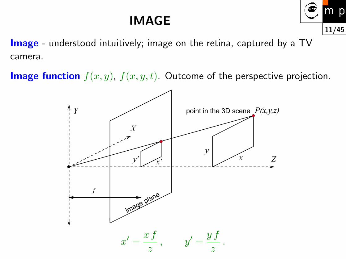
Image - understood intuitively; image on the retina, captured by a TV
camera.
Image function f(x, y), f(x, y, t). Outcome of the perspective projection.
Y P(x,y,z)
Z
X
y'y
x'x
image plane
f
point in the 3D scene
x′ =x f
z, y′ =
y f
z.

12/45IMAGE FUNCTION, 2-DIMENSIONAL SIGNAL
Monochromatic static image f(x, y), where
(x, y) are coordinates in a plane with domain
R = {(x, y), 1 ≤ x ≤ xm, 1 ≤ y ≤ yn} ;
f is image function value (≈ brightness, density of a transparent object,
distance to observer, etc.)
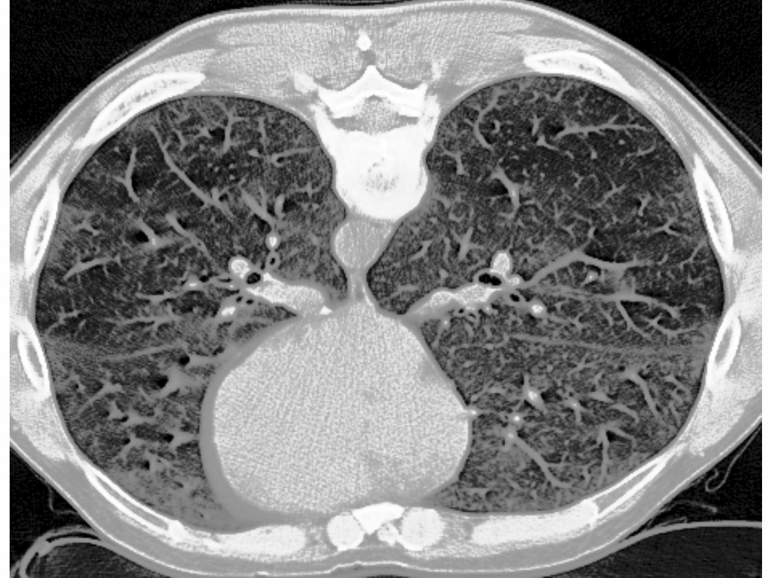
(Natural) 2D Images:
Thin specimen in optical microscope, image of a character on a paper,
finger print, a single cut from a tomograph, etc.

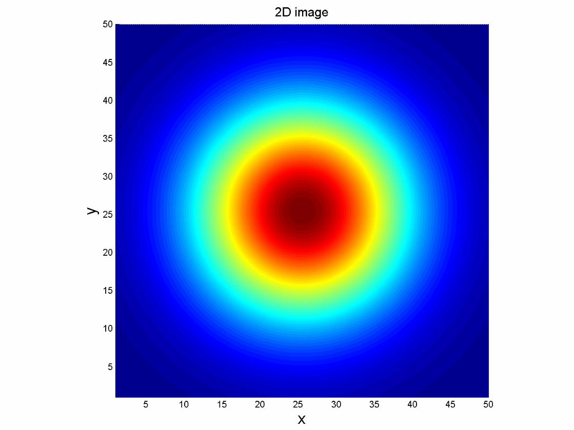
13/45IMAGE FUNCTION → DIGITAL IMAGE
From continuous to discrete space.
� Sampling of the image domain. Selection of dicrete points.
� Quantization of the image range. selection of disrete values.
� Usual representation = matrix. f(x, y) → f(r, c).
� Pixel = Picture element.
columns
row
s
Sampling 50x50, Quantization to 32 values
5 10 15 20 25 30 35 40 45 50
5
10
15
20
25
30
35
40
45
50

14/45SAMPLING
Two involved problems:
1. Arrangement of the sampling points.
(b)(a)
2. Distance between sampling points (Shannon sampling theorem).
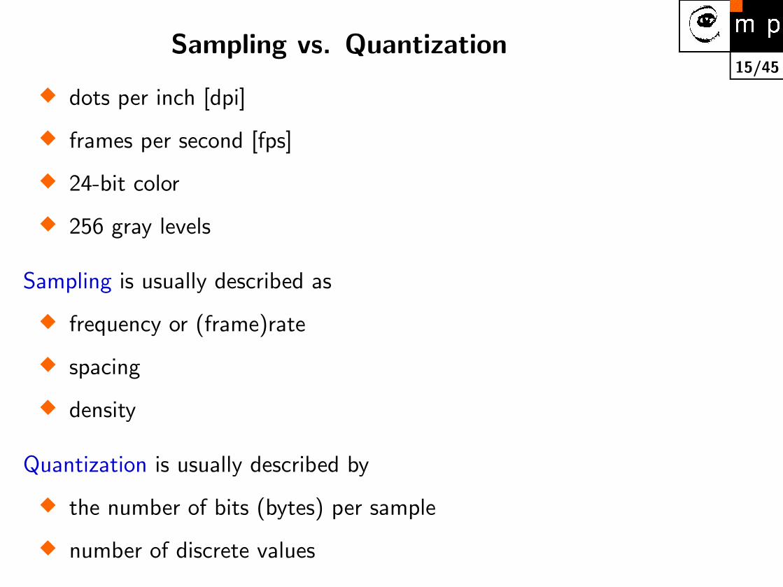
15/45Sampling vs. Quantization
� dots per inch [dpi]
� frames per second [fps]
� 24-bit color
� 256 gray levels
Sampling is usually described as
� frequency or (frame)rate
� spacing
� density
Quantization is usually described by
� the number of bits (bytes) per sample
� number of discrete values

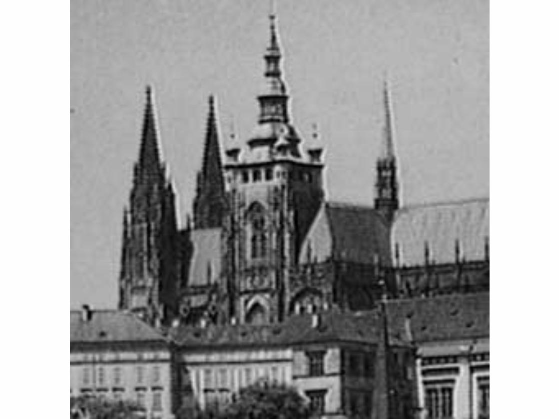
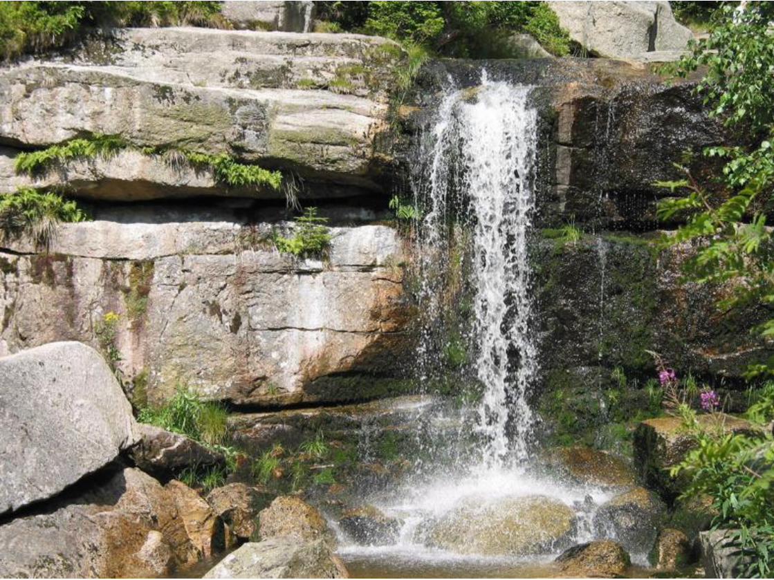
23/45Resolution
is the ability to distinguish between details. It is not the number of pixels.
Both images have the same number of pixels but different resolution. The
resolution is more related to what we can reconstruct from the image.

24/45DISTANCE
Function D is called the distance iff
D(p, q) ≥ 0 , particularly D(p, p) = 0 (identity).
D(p, q) = D(q, p) , (symmetry).
D(p, r) ≤ D(p, q) + D(q, r) , (triangular inequality).

25/45Several definitions of distance in a square raster
Euclidean distance (as the crow flies)
DE((x, y), (h, k)) =√
(x− h)2 + (y − k)2 .
City block distance (also called Manhattan distance)
D4((x, y), (h, k)) =| x− h | + | y − k | .
Chessboard distance
D8((x, y), (h, k)) = max{| x− h |, | y − k |} .
0
1
2
0 1 2 3 4
DE
D4
D8

26/454-neighbourhood and 8-neighbourhood
A set consisting of the pixel itself and its neighbours of distance 1.

28/45
BINARY IMAGE & RELATION ‘beingcontiguous’
black ∼ objects & white ∼ background
Neigbouring pixels are contiguous.
Two pixels are contiguous if there is a path between them consisting of
neigbouring pixels.

29/45REGION = compact set
Relation ’being contiguous’ is reflexive, symmetric, and transitive, i.e. this is
an equivalence relation.
Thus it decomposes the set of ’object’ pixels into equivalence classes =
regions.

30/45A FEW CONCEPTS
Boundary (of a region) vs. edge vs. edgel.
Inner and outer boundary.
Convex hull, lakes, bays.

31/45
Histogram of Image Intensities aka ImageHistogram
Histogram of image intensities is an estimate of probability density.
0 50 100 150 200 250
0
500
1000
1500
2000
2500
3000
3500
image histogram of intensities

32/45Histogram Equalization
The Aim:
� Increase contrast for a human observer.
� Normalize intensities for e.g., automatic image comparison
0 50 100 150 200 250
0
500
1000
1500
2000
2500
3000
3500
0 50 100 150 200 250
0
500
1000
1500
2000
2500
3000
3500
original histogram histogram after equalization

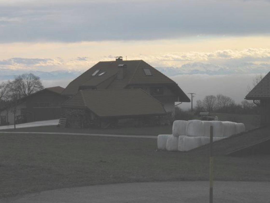
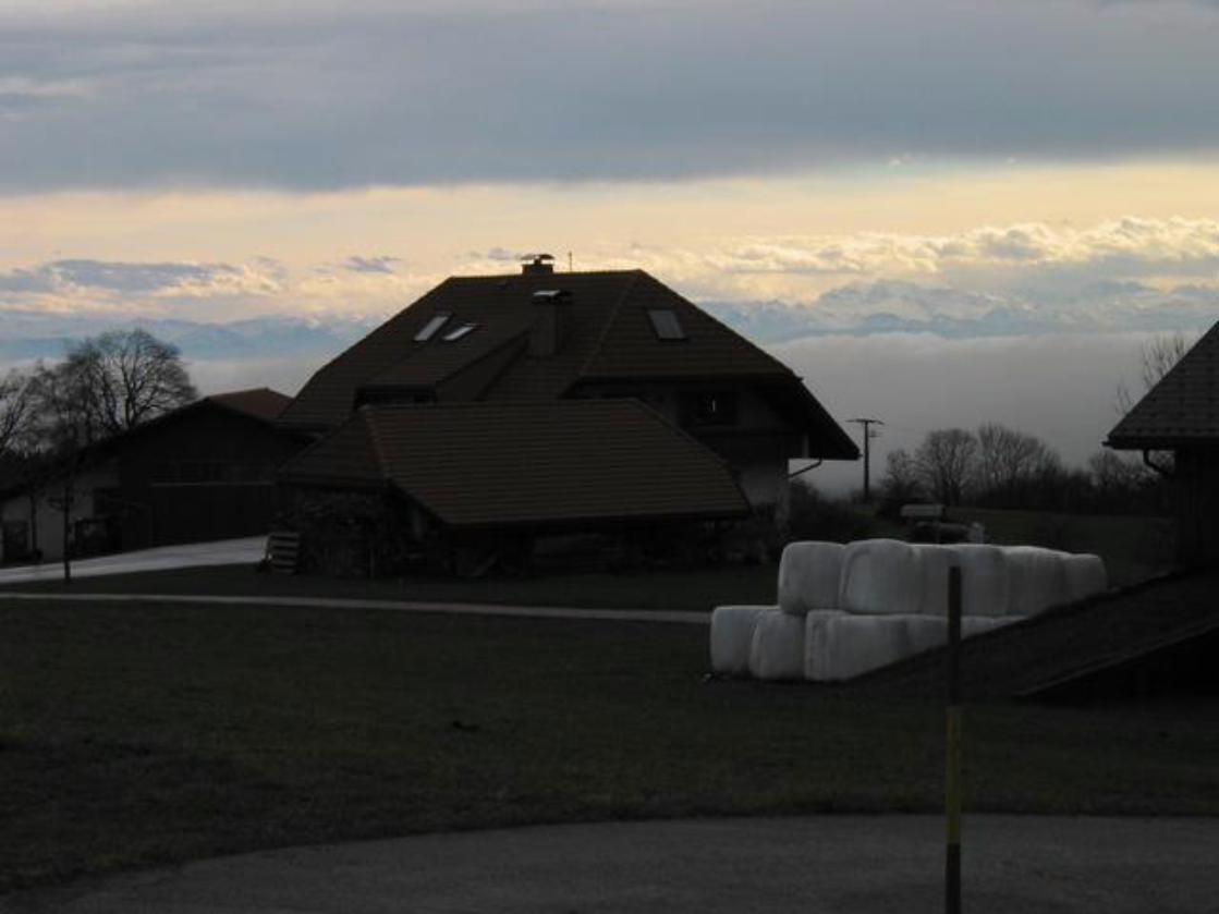
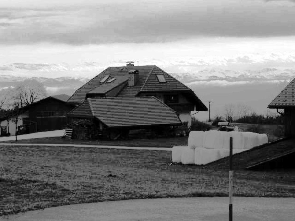
33/45Increased contrast after histogram equalization
original image . . . after equalization

34/45Histogram equalization — derivation
Input: histogram H(p) of the image with gray leveles p = 〈p0, pk〉.
Aim: find a monotonic pixel brightness transformation q = T (p), such that
the desired output histogram G(q) is uniform over the whole output
brightness scale q = 〈q0, qk〉.
The monotonicity of the transformation implies:
k∑i=0
G(qi) =k∑
i=0
H(pi) .
Equalized histogram ≈ uniform density
G(q) =N2
qk − q0.

35/45Histogram equalization — derivation II
The exactly uniform histogram may be obtained only in continuous space.∫ q
q0
G(s) ds =∫ p
p0
H(s) ds .

35/45Histogram equalization — derivation II
The exactly uniform histogram may be obtained only in continuous space.∫ q
q0
G(s) ds =∫ p
p0
H(s) ds .∫ q
q0
N2
qk − q0ds =
∫ p
p0
H(s) ds .

35/45Histogram equalization — derivation II
The exactly uniform histogram may be obtained only in continuous space.∫ q
q0
G(s) ds =∫ p
p0
H(s) ds .∫ q
q0
N2
qk − q0ds =
∫ p
p0
H(s) ds .
N2(q − q0)qk − q0
=∫ p
p0
H(s) ds .

35/45Histogram equalization — derivation II
The exactly uniform histogram may be obtained only in continuous space.∫ q
q0
G(s) ds =∫ p
p0
H(s) ds .∫ q
q0
N2
qk − q0ds =
∫ p
p0
H(s) ds .
N2(q − q0)qk − q0
=∫ p
p0
H(s) ds .
N2(q − q0) = (qk − q0)∫ p
p0
H(s) ds .

35/45Histogram equalization — derivation II
The exactly uniform histogram may be obtained only in continuous space.∫ q
q0
G(s) ds =∫ p
p0
H(s) ds .∫ q
q0
N2
qk − q0ds =
∫ p
p0
H(s) ds .
N2(q − q0)qk − q0
=∫ p
p0
H(s) ds .
N2(q − q0) = (qk − q0)∫ p
p0
H(s) ds .
q = T (p)

35/45Histogram equalization — derivation II
The exactly uniform histogram may be obtained only in continuous space.∫ q
q0
G(s) ds =∫ p
p0
H(s) ds .∫ q
q0
N2
qk − q0ds =
∫ p
p0
H(s) ds .
N2(q − q0)qk − q0
=∫ p
p0
H(s) ds .
N2(q − q0) = (qk − q0)∫ p
p0
H(s) ds .
q = T (p) =qk − q0
N2
∫ p
p0
H(s) ds + q0 .

36/45Histogram equalization — derivation III
Continous space distribution function
q = T (p) =qk − q0
N2
∫ p
p0
H(s) ds + q0 .
Dicrete space cumulative histogram
q = T (p) =qk − q0
N2
p∑i=p0
H(i) + q0 .

37/45More intensity transformations — original
0 50 100 150 200 250
0
500
1000
1500
2000
2500
3000
3500
4000
4500
5000

38/45
More intensity transformations — brightnessq = p + const
0 50 100 150 200 250
0
1000
2000
3000
4000
5000

39/45More intensity transformations — original
0 50 100 150 200 250
0
500
1000
1500
2000
2500
3000
3500
4000
4500
5000

40/45
More intensity transformations — contrastq = p ∗ const
0 50 100 150 200 250
0
1000
2000
3000
4000
5000

41/45More intensity transformations — original
0 50 100 150 200 250
0
500
1000
1500
2000
2500
3000
3500
4000
4500
5000

42/45
More intensity transformations — gammacorrected q = pγ
0 50 100 150 200 250
0
500
1000
1500
2000
2500
3000
3500
4000

43/45More intensity transformations — original
0 50 100 150 200 250
0
500
1000
1500
2000
2500
3000
3500
4000
4500
5000
44/45
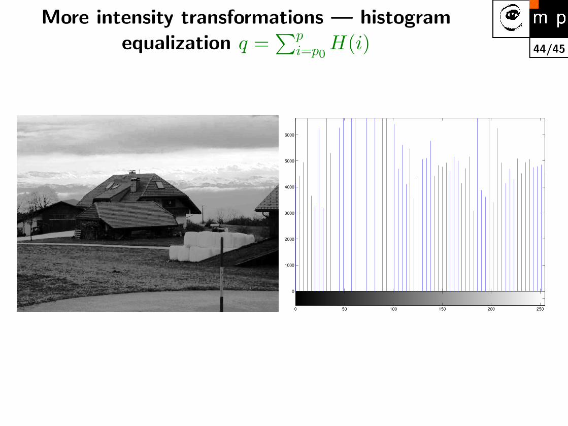
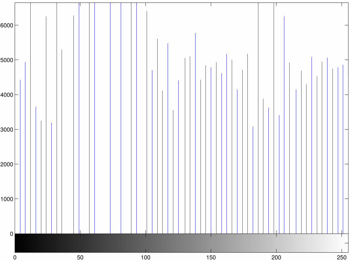
More intensity transformations — histogramequalization q =
∑pi=p0
H(i)
0 50 100 150 200 250
0
1000
2000
3000
4000
5000
6000


Objector scene
2D image
Digitalimage
Regions Edgels Scale Orientation Texture
Image withfeatures
Objects
from objects to images
from images to features
from features to objects
understanding objects

Y P(x,y,z)
Z
X
y'y
x'x
image plane
f
point in the 3D scene


columns
row
s
Sampling 50x50, Quantization to 32 values
5 10 15 20 25 30 35 40 45 50
5
10
15
20
25
30
35
40
45
50

(b)(a)


0
1
2
0 1 2 3 4
DE
D4
D8


0 50 100 150 200 250
0
500
1000
1500
2000
2500
3000
3500

0 50 100 150 200 250
0
500
1000
1500
2000
2500
3000
3500

0 50 100 150 200 250
0
500
1000
1500
2000
2500
3000
3500


0 50 100 150 200 250
0
500
1000
1500
2000
2500
3000
3500
4000
4500
5000

0 50 100 150 200 250
0
1000
2000
3000
4000
5000


0 50 100 150 200 250
0
500
1000
1500
2000
2500
3000
3500
4000
4500
5000


0 50 100 150 200 250
0
1000
2000
3000
4000
5000


0 50 100 150 200 250
0
500
1000
1500
2000
2500
3000
3500
4000
4500
5000


0 50 100 150 200 250
0
500
1000
1500
2000
2500
3000
3500
4000

0 50 100 150 200 250
0
500
1000
1500
2000
2500
3000
3500
4000
4500
5000
0 50 100 150 200 250
0
1000
2000
3000
4000
5000
6000


![Rudolf S´ykora and Tom´aˇs Novotn´y1, Department of Condensed … · 2018-10-21 · arXiv:1705.03719v1 [cond-mat.mes-hall] 10 May 2017 Graph-theoretical evaluation of the inelastic](https://img.pdfslide.us/doc/110x75/5f98d71c8b875114ec0c0d48/rudolf-sykora-and-tomas-novotny1-department-of-condensed-2018-10-21-arxiv170503719v1.jpg)