Embed Size (px)
Citation preview

Introduction to Discrete Element Methods
Basics of Contact Force Models and how to performthe Micro-Macro Transition to Continuum Theory
Stefan Luding
Multi Scale Mechanics, TS, CTW, UTwente,P.O.Box 217, 7500 AE Enschede, Netherlands
ABSTRACT.One challenge of todays research is the realistic simulation of granular materials,like sand or powders, consisting of millions of particles. In this article, the discrete elementmethod (DEM), as based on molecular dynamics methods, is introduced.Contact models are at the physical basis of DEM. A set of the most basic force models is pre-sented involving either elasto-plasticity, adhesion, viscosity, static and dynamic friction as wellas rolling- and torsion-resistance.The examples given concern clustering in granular gases, and bi-axial as well as cylindricalshearing of dense packings in order to illustrate the micro-macro transition towards continuumtheory.
RÉSUMÉ.Un des grand défis de la recherche d’aujourd’hui est de pouvoir simuler de manièreréaliste les matériaux granulaires comme le sable ou les poudres qui sont constituées de mil-lions de particules. La méthode des éléments discrets (DEM en anglais), basée sur le conceptde la méthode de dynamique moléculaire, est introduite.Les modèles de contacts sont á la base de la méthode des éléments discrets (DEM). Une sériede modèles de base est présenté avec des interactions de typeélasto-plastiques, adhésives, vis-queuses, des contacts à frottements statique et dynamique ainsi que des contacts résistant enroulement et torsion.Des exemples de simulations des gaz granulaires “clustering” et glissements bi-axiaux et cylin-driques dans des systèmes denses sont étudiés afin d’illustrer le passage du discret au continu.
KEYWORDS:granular matter, molecular dynamics (MD), discrete element methods (DEM), eventdriven MD, iparallelization, equation of state, clustering, shear bands, micro-macro transition
MOTS-CLÉS :matériaux granulaires, dynamique moléculaire, “event-driven MD”, parallélisa-tion, équation d’état, “clustering”, bandes de glissement, “micro-macro transition”
EJECE – 12/2008. Discrete modelling of geomaterials, pages785 à 826

786 EJECE – 12/2008. Discrete modelling of geomaterials
1. Introduction
The approach towards the microscopic understanding of macroscopic particulatematerial behavior (Herrmann, 1997; Kishino, 2001; Hinrichsenet al., 2004) is themodeling of particles using so-called discrete element methods (DEM). Even thoughmillions of particles can be simulated, the possible lengthof such a particle systemis in general too small in order to regard it as macroscopic. Therefore, methods andtools to perform a so-called micro-macro transition (Vermeer et al., 2001; Pöscheletal., 2001; Kirkwoodet al., 1949) are discussed, starting from the DEM simulations.These “microscopic” simulations of a small sample (representative volume element)can be used to derive macroscopic constitutive relations needed to describe the mate-rial within the framework of a macroscopic continuum theory.
For granular materials, as an example, the particle properties and interaction lawsare inserted into DEM, which is also often referred to as molecular dynamics (MD),and lead to the collective behavior of the dissipative many-particle system. From aparticle simulation, one can extract,e.g., the pressure of the system as a function ofdensity. This equation of state allows a macroscopic description of the material, whichcan be viewed as a compressible, non-Newtonian complex fluid(Ludinget al., 2001b),including a fluid-solid phase transition.
In the following, two versions of the molecular dynamics simulation method areintroduced. The first is the so-called soft sphere moleculardynamics (MD=DEM),as described in Section 2. It is a straightforward implementation to solve the equa-tions of motion for a system of many interacting particles (Allen et al., 1987; Rapa-port, 1995). For DEM, both normal and tangential interactions, like friction, are dis-cussed for spherical particles. The second method is the so-called event-driven (ED)simulation, as discussed in Section 3, which is conceptually different from DEM,since collisions are dealt with using a collision matrix that determines the momentumchange on physical grounds. For the sake of brevity, the ED method is only discussedfor smooth spherical particles. A comparison and a way to relate the soft and hardparticle methods is provided in Section 4.
As one ingredient of a micro-macro transition, the stress isdefined for a dynamicsystem of hard spheres, in Section 5, by means of kinetic-theory arguments (Pöschelet al., 2001), and for a quasi-static system by means of volume averages (Lätzeletal., 2000). Examples are presented in the following Sections 6 and 7, where the above-described methods are applied.
2. The soft particle Molecular Dynamics (MD) method
One possibility to obtain information about the behavior ofgranular media is toperform experiments. An alternative are simulations with the molecular dynamics(MD) or discrete element model (DEM) (Cundallet al., 1979; Bashiret al., 1991; vanBaars, 1996; Herrmannet al., 1998; Thornton, 2000; Thorntonet al., 2000; Thorntonet al., 2001; Vermeeret al., 2001; Lätzelet al., 2003). Note that both methods are

Introduction to discrete element methods 787
identical in spirit, however, different groups of researchers use these (and also other)names.
Conceptually, the DEM method has to be separated from the hard sphere event-driven (ED) molecular dynamics, see Section 3, and also fromthe so-called ContactDynamics (CD). The former will be discussed below and in the article by T. Pöschelin this book, the latter (CD) will be introduced in the article by F. Radjai in this book.Alternative stochastic methods like cell- or lattice gas-methods are just named as key-words, but not discussed here at all.
2.1. Discrete Element Model (DEM)
The elementary units of granular materials are mesoscopic grains which deformunder stress. Since the realistic modeling of the deformations of the particles is muchtoo complicated, we relate the interaction force to the overlap δ of two particles, seeFigure 1. Note that the evaluation of the inter-particle forces based on the overlapmay not be sufficient to account for the inhomogeneous stressdistribution inside theparticles. Consequently, our results presented below are of the same quality as thesimple assumptions about the force-overlap relation, see Figure 1.
2.2. Equations of motion
If all forcesf i acting on the particlei, either from other particles, from bound-aries or from external forces, are known, the problem is reduced to the integration ofNewton’s equations of motion for the translational and rotational degrees of freedom:
mid2
dt2ri = f i +mig , and Ii
d
dtωi = ti [1]
with the massmi of particlei, its positionri the total forcef i =∑
c fci acting on it
due to contacts with other particles or with the walls, the acceleration due to volumeforces like gravityg, the spherical particles moment of inertiaIi, its angular velocityωi and the total torqueti =
∑
c (lci × f ci + qc
i ), whereqci are torques/couples at
contacts other than due to a tangential force,e.g., due to rolling and torsion.
The equations of motion are thus a system ofD + D(D − 1)/2 coupled ordinarydifferential equations to be solved inD = 2, 3 dimensions. With tools from numericalintegration, as nicely described in textbooks as (Allenet al., 1987; Rapaport, 1995),this is straightforward. The typically short-ranged interactions in granular media, al-low for a further optimization by using linked-cell or alternative methods (Allenetal., 1987; Rapaport, 1995) in order to make the neighborhood search more efficient.In the case of long-range interactions, (e.g.charged particles with Coulomb interac-tion, or objects in space with self-gravity) this is not possible anymore, so that moreadvanced methods for optimization have to be applied – for the sake of brevity, werestrict ourselves to short range interactions here.

788 EJECE – 12/2008. Discrete modelling of geomaterials
δ
r
ri
j
δ
k1δ
−k
(δ−δ )*2 0k
δmax
f hys
minδ
minf
f0
0
δ0
cδ
Figure 1. (Left) two particle contact with overlapδ . (Right) schematic graph of thepiecewise linear, hysteretic, adhesive force-displacement model used below
2.3. Normal contact force laws
2.3.1. Linear normal contact model
Two spherical particlesi andj, with radii ai andaj , respectively, interact only ifthey are in contact so that their overlap
δ = (ai + aj) − (ri − rj) · n [2]
is positive,δ > 0, with the unit vectorn = nij = (ri − rj)/|ri − rj | pointing fromj to i. The force on particlei, from particlej, at contactc, can be decomposed into anormal and a tangential part asfc := fc
i = fnn + f tt, wherefn is discussed first.
The simplest normal contact force model, which takes into account excluded vol-ume and dissipation, involves a linear repulsive and a linear dissipative force
fn = kδ + γ0vn [3]
with a spring stiffnessk, a viscous damping coefficientγ0, and the relative velocity innormal directionvn = −vij · n = −(vi − vj) · n = δ.
This so-called linear spring dashpot model allows to view the particle contact as adamped harmonic oscillator, for which the half-period of a vibration around an equi-librium position, see Figure 1, can be computed, and one obtains a typical responsetime on the contact level,
tc =π
ω, with ω =
√
(k/m12) − η20 [4]
with the eigenfrequency of the contactω, the rescaled damping coefficientη0 =γ0/(2mij), and the reduced massmij = mimj/(mi + mj). From the solution of

Introduction to discrete element methods 789
the equation of a half period of the oscillation, one also obtains the coefficient ofrestitution
r = −v′n/vn = exp (−πη0/ω) = exp (−η0tc) [5]
which quantifies the ratio of relative velocities after (primed) and before (unprimed)the collision. For a more detailed discussion of this and other, more realistic, non-linear contact models, seee.g.(Luding, 1998), and the articles by Pöschel and Radjaiin this book.
The contact duration in Equation [4] is also of practical technical importance, sincethe integration of the equations of motion is stable only if the integration time-step∆tDEM is much smaller thantc. Furthermore, it depends on the magnitude of dis-sipation. In the extreme case of an overdamped spring,tc can become very large.Therefore, the use of neither too weak nor too strong dissipation is recommended.
2.3.2. Adhesive, elasto-plastic normal contact model
Here we apply a variant of the linear hysteretic spring model(Waltonet al., 1986;Luding, 1998; Tomas, 2000; Luding, 2008a), as an alternative to the frequently appliedspring-dashpot models. This model is the simplest version of some more complicatednonlinear-hysteretic force laws (Waltonet al., 1986; Zhuet al., 1991; Saddet al.,1993), which reflect the fact that at the contact point, plastic deformations may takeplace. The repulsive (hysteretic) force can be written as
fhys =
k1δ for loading, if k∗2(δ − δ0) ≥ k1δk∗2(δ − δ0) for un/reloading, if k1δ > k∗2(δ − δ0) > −kcδ−kcδ for unloading, if − kcδ ≥ k∗2(δ − δ0)
[6]
with k1 ≤ k∗2 , see Figure 1, and Equation [7] below for the definition of the(variable)k∗2 as function of the constant model parameterk2.
During the initial loading the force increases linearly with the overlapδ, untilthe maximum overlapδmax is reached (which has to be kept in memory as a historyparameter). The line with slopek1 thus defines the maximum force possible for agiven δ. During unloading the force drops from its value atδmax down to zero atoverlapδ0 = (1 − k1/k
∗
2)δmax, on the line with slopek∗2 . Reloading at any instantleads to an increase of the force along this line, until the maximum force is reached;for still increasingδ, the force follows again the line with slopek1 andδmax has to beadjusted accordingly.
Unloading belowδ0 leads to negative, attractive forces until the minimum force−kcδmin is reached at the overlapδmin = (k∗2 − k1)δmax/(k
∗
2 + kc). This mini-mum force,i.e. the maximum attractive force, is obtained as a function of the modelparametersk1, k2, kc, and the history parameterδmax. Further unloading leads toattractive forcesfhys = −kcδ on the adhesive branch with slope−kc. The high-est possible attractive force, for givenk1 andk2, is reached forkc → ∞, so that

790 EJECE – 12/2008. Discrete modelling of geomaterials
fhysmax = −(k2 − k1)δmax. Since this would lead to a discontinuity atδ = 0, it is
avoided by using finitekc.
The lines with slopek1 and−kc define the range of possible force values anddeparture from these lines takes place in the case of unloading and reloading, respec-tively. Between these two extremes, unloading and reloading follow the same linewith slopek2. Possible equilibrium states are indicated as circles in Figure 1, wherethe upper and lower circle correspond to a pre-stressed and stress-free state, respec-tively. Small perturbations lead, in general, to small deviations along the line withslopek2 as indicated by the arrows.
A non-linear un/reloading behavior would be more realistic, however, due to alack of detailed experimental informations, we use the piece-wise linear model as acompromise. One refinement is ak∗2 value dependent on the maximum overlap thatimplies small and large plastic deformations for weak and strong contact forces, re-spectively. One model, as implemented recently (Ludinget al., 2005; Luding, 2008a),requires an additional model parameter,δ∗max, so thatk∗2(δmax) is increasing fromk1
to k2 (linear interpolation is used below, however, this is another choice to be madeand will depend on the material under consideration) with the maximum overlap, untilδ∗max is reached1:
k∗2(δmax) =
k2 if δmax ≥ δ∗max
k1 + (k2 − k1)δmax/δ∗
max if δmax < δ∗max
[7]
While in the case of collisions of particles with large deformations, dissipationtakes place due to the hysteretic nature of the force-law, stronger dissipation of smallamplitude deformations is achieved by adding the viscous, velocity dependent dissi-pative force from Equation [3] to the hysteretic force, suchthatfn = fhys + γ0vn.The hysteretic model contains the linear contact model as special casek1 = k2 = k.
2.3.3. Long range normal forces
Medium range van der Waals forces can be taken into account inaddition to thehysteretic force such thatfn = fhys
i + fvdWi with, for example, the attractive part of
a Lennard-Jones Potential
fvdW = −6(ε/r0)[(r0/rij)7 − (r0/rc)
7] for rij ≤ rc . [8]
The new parameters necessary for this force are an energy scale ε, a typical lengthscaler0 and a cut-off lengthrc. As long asrc is not much larger than the particle di-ameter, the methods for short range interactions still can be applied to such a mediumrange interaction model – only the linked cells have to be larger than twice the cut-offradius, and no force is active forr > rc.
1. A limit to the slopek2 is needed for practical reasons. Ifk2 would not be limited, thecontact duration could become very small so that the time step would have to be reduced belowreasonable values.

Introduction to discrete element methods 791
2.4. Tangential forces and torques in general
For the tangential degrees of freedom, there are three different force- and torque-laws to be implemented: (i) friction, (ii) rolling resistance, and (iii) torsion resistance.
2.4.1. Sliding
For dynamic (sliding) and staticfriction, the relative tangential velocity of thecontact points,
vt = vij − n(n · vij) [9]
is to be considered for the force and torque computations in subsection 2.5, with thetotal relative velocity of the particle surfaces at the contact
vij = vi − vj + a′in × ωi + a′jn × ωj [10]
with the corrected radius relative to the contact pointa′α = aα − δ/2, for α = i, j.Tangential forces acting on the contacting particles are computed from the accumu-lated sliding of the contact points along each other, as described in detail in Section2.5.1.
2.4.2. Objectivity
In general, two particles can rotate together, due to both a rotation of the referenceframe or a non-central “collision”. The angular velocityω0 = ωn
0 +ωt0, of the rotating
reference has the tangential-plane component
ωt0 =
n × (vi − vj)
a′i + a′j[11]
which is related to the relative velocity, while the normal component,ωn0 , is not.
Insertingωi = ωj = ωt0, from Equation [11], into Equation [10] leads to zero sliding
velocity, proving that the above relations are objective. Tangential forces and torquesdue to sliding can become active only when the particles are rotating with respect tothe common rotating reference frame2.
Since action should be equal to reaction, the tangential forces are equally strong,but opposite,i.e., f t
j = −f ti, while the corresponding torques are parallel but not nec-
essarily equal in magnitude:qfrictioni = −a′in × f i, andqfriction
j = (a′j/a′
i)qfrictioni .
Note that tangential forces and torquestogetherconserve the total angular momentumabout the pair center of mass
Lij = Li + Lj +mir2icmωt
0 +mjr2jcmωt
0 [12]
2. For rolling and torsion, there is no similar relation between rotational and tangential degreesof freedom: for any rotating reference frame, torques due torolling and torsion can becomeactive only due to rotation relative to the common referenceframe, see below.

792 EJECE – 12/2008. Discrete modelling of geomaterials
with the rotational contributionsLα = Iαωα, for α = i, j, and the distancesrαcm =|rα−rcm| from the particle centers to the center of massrcm = (miri+mjrj)/(mi+mj), see (Luding, 1998). The change of angular momentum consists of the changeof particle spins (first term) and of the change of the angularmomentum of the twomasses rotating about their common center of mass (second term):
dLij
dt= qfriction
i
(
1 +a′ja′i
)
+(
mir2icm +mjr
2jcm
) dωt0
dt[13]
which both contribute, but exactly cancel each other, since
qfrictioni
(
1 +a′ja′i
)
= −(a′i + a′j)n × f i [14]
= −(
mir2icm +mjr
2jcm
) dωt0
dt
see (Luding, 2006) for more details.
2.4.3. Rolling
A rolling velocityv0r = −a′in×ωi + a′jn×ωj, defined in analogy to the sliding
velocity, is not objective in general (Els, 2006; Luding, 2006) – only in the specialcases of (i) equal-sized particles or (ii) for a particle rolling on a fixed flat surface.
The rolling velocity should quantify the distance the two surfaces roll over eachother (without sliding). Therefore, it is equal for both particles by definition. Anobjective rolling velocityis obtained by using the reduced radius,a′ij = a′ia
′
j/(a′
i +a′j), so that
vr = −a′ij (n × ωi − n × ωj) . [15]
This definition is objective since any common rotation of thetwo particles vanishesby construction. A more detailed discussion of this issue isbeyond the scope of thispaper, rather see (Els, 2006; Luding, 2006) and the references therein.
A rolling velocity will activate torques, acting against the rolling motion,e.g.,when two particles are rotating anti-parallel with spins inthe tangential plane. Thesetorques are then equal in magnitude and opposite in direction, i.e., q
rollingi =
−qrollingj = aij n × fr, with the quasi-forcefr, computed in analogy to the fric-
tion force, as function of the rolling velocityvr in Section 2.5.2; the quasi-forces forboth particles are equal and do not act on the centers of mass.Therefore, the totalmomenta (translational and angular) are conserved.
2.4.4. Torsion
For torsion resistance, the relative spin along the normal direction
vo = aij (n · ωi − n · ωj)n [16]

Introduction to discrete element methods 793
is to be considered, which activates torques when two particles are rotating anti-parallel with spins parallel to the normal direction. Torsion is not activated by a com-mon rotation of the particles around the normal directionn · ω0 = n · (ωi + ωj) /2,which makes the torsion resistance objective.
The torsion torques are equal in magnitude and directed in opposite directions,i.e.,qtorsion
i = −qtorsionj = aij fo, with the quasi-forcef o, computed from the torsion
velocity in Section 2.5.3, and also not changing the translational momentum. Like forrolling, the torsion torques conserve the total angular momentum.
2.4.5. Summary
The implementation of the tangential force computations for f t, fr, andf o asbased onvt, vr, andvo, respectively, is assumed to beidentical, i.e., even the samesubroutine is used, but with different parameters as specified below. The difference isthat friction leads to a force in the tangential plane (changing both translational andangular momentum), while rolling- and torsion-resistancelead to quasi-forces in thetangential plane and the normal direction, respectively, changing the particles’ angularmomentum only. For more details on tangential contact models, friction, rolling andtorsion, see (Bartelset al., 2005; Dintwaet al., 2005; Luding, 2007; Luding, 2006;Els, 2006).
2.5. The tangential force- and torque-models
The tangential contact model presented now is a single procedure (subroutine) thatcan be used to compute either sliding, rolling, or torsion resistance. The subroutineneeds a relative velocity as input and returns the respective force or quasi-force asfunction of the accumulated deformation. The sliding/sticking friction model will beintroduced in detail, while rolling and torsion resistanceare discussed where different.
2.5.1. Sliding/sticking friction model
The tangential force is coupled to the normal force through Coulomb’s law,f t ≤fs
C := µsfn, where for the sliding case one has dynamic friction withf t = f tC :=
µdfn. The dynamic and the static friction coefficients follow, ingeneral, the relationµd ≤ µs. The static situation requires an elastic spring in order toallow for a restoringforce,i.e., a non-zero remaining tangential force in static equilibrium due to activatedCoulomb friction.
If a purely repulsive contact is established,fn > 0, and the tangential force isactive. For an adhesive contact, Coulombs law has to be modified in so far thatfn isreplaced byfn + kcδ. In this model, the reference for a contact is no longer the zeroforce level, but it is the adhesive, attractive force level along−kcδ.

794 EJECE – 12/2008. Discrete modelling of geomaterials
If a contact is active, one has to project (or better rotate) the tangential spring into theactual tangential plane, since the frame of reference of thecontact may have rotatedsince the last time-step. The tangential spring
ξ = ξ′ − n(n · ξ′) [17]
is used for the actual computation, whereξ′ is the old spring from the last iteration,with |ξ| = |ξ′| enforced by appropriate scaling/rotation. If the spring isnew, thetangential spring-length is zero, but its change is well defined after the first, initiationstep. In order to compute the changes of the tangential spring, a tangential test-force isfirst computed as the sum of the tangential spring force and a tangential viscous force(in analogy to the normal viscous force)
f t0 = −kt ξ − γtvt [18]
with the tangential spring stiffnesskt, the tangential dissipation parameterγt, andvt
from Equation [9]. As long as|f t0| ≤ fs
C , with fsC = µs(fn + kcδ), one has static
friction and, on the other hand, for|f t0| > fs
C , sliding friction becomes active. Assoon as|f t
0| gets smaller thanfdC , static friction becomes active again.
In thestatic frictioncase, below the Coulomb limit, the tangential spring is incre-mented
ξ′ = ξ + vt ∆tMD [19]
to be used in the next iteration in Equation [17], and the tangential forcef t = f t0 from
Equation [18] is used. In thesliding friction case, the tangential spring is adjusted toa length consistent with Coulombs condition, so that
ξ′ = − 1
kt
(
fdC t + γtvt
)
[20]
with the tangential unit vector,t = f t0/|f t
0|, defined by Equation [18], and thusthe magnitude of the Coulomb force is used. Insertingξ′ from Equation [20] intoEquation [18] during the next iteration will lead tof t
0 ≈ fdCt. Note thatf t
0 andvt arenot necessarily parallel in three dimensions. However, themapping in Equation [20]works always, rotating the new spring such that the direction of the frictional force isunchanged and, at the same time, limiting the spring in length according to Coulombslaw. In short notation the tangential contact law reads
f t = f tt = +min(
fC , |f t0|
)
t [21]
wherefC follows the static/dynamic selection rules described above. The torque on aparticle due to frictional forces at this contact isqfriction = lci × fc
i , wherelci is thebranch vector, connecting the center of the particle with the contact point. Note thatthe torque on the contact partner is generally different in magnitude, sincelci can bedifferent, but points in the same direction; see Section 2.4.2 for details on this.

Introduction to discrete element methods 795
The four parameters for the friction law arekt,µs, φd = µd/µs, andγt, accountingfor tangential stiffness, the static friction coefficient,the dynamic friction ratio, andthe tangential viscosity, respectively. Note that the tangential force described above isidentical to the classical Cundall-Strack spring only in the limits µ = µs = µd, i.e.,φd = 1, andγt = 0. The sequence of computations and the definitions and mappingsinto the tangential direction can be used in 3D as well as in 2D.
2.5.2. Rolling resistance model
The three new parameters for rolling resistance arekr, µr, andγr, whileφr = φd
is used from the friction law. The new parameters account forrolling stiffness, astatic rolling “friction” coefficient, and rolling viscosity, respectively. In the subrou-tine called, the rolling velocityvr is used instead ofvt and the computed quasi-forcefr is used to compute the torques,qrolling, on the particles.
2.5.3. Torsion resistance model
The three new parameters for rolling resistance areko, µo, andγo, whileφo = φd
is used from the friction law. The new parameters account fortorsion stiffness, a statictorsion “friction” coefficient, and torsion viscosity, respectively. In the subroutine,the torsion velocityvo is used instead ofvt and the projection is a projection alongthe normal unit-vector, not into the tangential plane as forthe other two models. Thecomputed quasi-forcef o is then used to compute the torques,qtorsion, on the particles.
2.6. Background friction
Note that the viscous dissipation takes place in a two-particle contact. In the bulkmaterial, where many particles are in contact with each other, this dissipation modeis very inefficient for long-wavelength cooperative modes of motion (Ludinget al.,1994b; Ludinget al., 1994a). Therefore, an additional damping with the backgroundcan be introduced, so that the total force on particlei is
f i =∑
j
(
fnn + f tt)
− γbvi [22]
and the total torque
qi =∑
j
(
qfriction + qrolling + qtorsion)
− γbra2i ωi [23]
with the damping artificially enhanced in the spirit of a rapid relaxation and equili-bration. The sum in Equations [22] and [23] takes into account all contact partnersjof particlei, but the background dissipation can be attributed to the medium betweenthe particles. Note that the effect ofγb andγbr should be checked for each set ofparameters: it should be small in order to exclude artificialover-damping. The set ofparameters is summarized in Table 1. Note that only a few parameters are specifiedwith dimensions, while the other paramters are expressed asratios.

796 EJECE – 12/2008. Discrete modelling of geomaterials
Table 1. Summary of the microscopic contact model parameters. The longer rangedforces and their parameters,ǫ, r0, andrc are not included here
Property Symbol
Time unit tuLength unit xu
Mass unit mu
Particle radius a0
Material density ρElastic stiffness (variable) k∗2Maximal elastic stiffness k := k2
Plastic stiffness k1/kAdhesion “stiffness” kc/kFriction stiffness kt/kRolling stiffness kr/kTorsion stiffness ko/kPlasticity depth φf
Coulomb friction coefficient µ = µd = µs
Dynamic to static Friction ratio φd = µd/µs
Rolling “friction” coefficient µr
Torsion “friction” coefficient µo
Normal viscosity γ = γn
Friction viscosity γt/γRolling viscosity γr/γTorsion viscosity γo/γBackground viscosity γb/γBackground viscous torque γbr/γ
2.7. Example: tension test simulation results
In order to illustrate the power of the contact model (especially the adhesive normalmodel), in this Section, uni-axial tension and compressiontests are presented. Notethat the contact model parameters are chosen once and then one can simulate looseparticles, pressure-sintering, and agglomerates with oneset of paramters. With slightextensions, the same model was already applied to temperature-sintering (Ludingetal., 2005) or self-healing (Ludinget al., 2007; Ludinget al., 2008).
The tests consists of three stages: (i) pressure sintering,(ii) stress-relaxation, and(iii) the compression- or tension-test itself. The contactparameters, as introducedin the previous Section, are summarized in Table 1 and typical values are given inTable 2. These parameters are used for particle-particle contacts,the same for alltests, unless explicitly specified.

Introduction to discrete element methods 797
First, forpressure sintering, a very loose assembly of particles is compressed withisotropic stressps2a/k2 ≈ 0.02 in a cuboidal volume so that the adhesive contactforces are activated this way. The stress- and strain-controlled wall motion modesaredescribed below in Section 6.2.2.
Two of the six walls are adhesive, withkwallc /k2 = 20, so that the sample sticks to
them later, while all other walls are adhesionless, so that they can be easily removedin the next step. Note that during compression and sintering, the walls could all bewithout adhesion, since the high pressure used keeps the sample together anyway –only later for relaxation, adhesion must switched on. If notthe sample does not remaina solid, and it also could lose contact with the walls, which are later used to apply thetensile strain.
All walls should be frictionless during sintering, while the particles can be slightlyadhesive and frictional. If the walls would be frictional, the pressure from a certainwall would not be transferred completely to the respective opposite wall, since fric-tional forces carry part of the load – an effect that is known since the early work ofJanssen (Janssen, 1895; Sperl, 2006; Tigheet al., 2007). Pressure-sintering is stoppedwhen the kinetic energy of the sample is many orders of magnitude smaller than thepotential energy – typically 10 orders of magnitude.
During stress-relaxationall wall stresses are slowly released topr/ps ≪ 1 andthe sample is relaxed again until the kinetic energy is much smaller than the potentialenergy. After this, the sample is ready for thetension or compression tests. Thenon-adhesive side walls still feel a very small external stress that is not big enough toaffect the dynamics of the tension test, it is just convenient to keep the walls close tothe sample. (This is a numerical and not a physical requirement, since our code useslinked-cells and those are connected to the system size. If the walls would move toofar away, either the linked cells would grow, or their numberwould increase. Bothcases are numerically inefficient.)
For thetension testwall friction is typically active, but some variation does notshow a big effect. One of the sticky walls is slowly and smoothly moved outwardslike described and applied in earlier studies (Ludinget al., 2001a; Luding, 2005a;Luding, 2007; Ludinget al., 2007; Luding, 2008a; Ludinget al., 2008), following aprescribed cosine-function with time.
2.7.1. Model parameters for tension
The system presented here containsN = 1728 particles with radiiai drawn froma Gaussian distribution arounda = 0.005mm (Davidet al., 2005; Davidet al., 2007).The contact model parameters are summarized in Tables 1 and 2. The volume frac-tion, ν =
∑
i V (ai)/V , with the particle volumeV (ai) = (4/3)πa3i , reached during
pressure sintering with2aps/k2 = 0.01 is νs = 0.6754. The coordination number isC ≈ 7.16 in this state. After stress-relaxation, these values have changed toν ≈ 0.629andC ≈ 6.19. A different preparation procedure (with adhesionkc/k2 = 0 duringsintering) does not lead to a difference in density after sintering.

798 EJECE – 12/2008. Discrete modelling of geomaterials
Table 2. Microscopic material parameters used (second column), if not explicitlyspecified. The third column contains these values in the appropriate units,i.e., whenthe time-, length-, and mass-unit areµs, mm, and mg, respectively. Column four con-tains the parameters in SI-units. Energy, force, acceleration, and stress have to bescaled with factors of 1, 103, 109, and 109, respectively, for a transition from reducedto SI-units
Symbol Value rescaled units SI-units
tu 1 1µs 10−6 sxu 1 1 mm 10−3 mmu 1 1 mg 10−6 kga0 0.005 5µm 5.10−6mρ 2 2 mg/mm3 2000 kg/m3
k := k2 5 5 mg/µs2 5.106 kg/s2
k1/k 0.5 - -kc/k 0.5 - -kt/k 0.2 - -kr/k = ko/k 0.1 - -φf 0.05 - -µ = µd = µs 1 - -φd = µd/µs 1 - -µr = µo 0.1 - -γ = γn 5.10−5 5.10−5 mg/µs 5.101 kg/sγt/γ 0.2 - -γr/γ = γo/γ 0.05 - -γb/γ 4.0 - -γbr/γ 1.0 - -
However, one observesν ≈ 0.630 andC ≈ 6.23 after relaxation. For both prepa-ration procedures the tension test results are virtually identical, so that only the firstprocedure is used in the following.
The material parameters used for the particle contacts are given in Table 2. Theparticle-wall contact parameters are the same, except for cohesion and friction, forwhichkwall
c /k2 = 20 andµwall = 10 are used – the former during all stages, the latteronly during tensile testing.
The choice of numbers and units is such that the particles correspond spheres withseveral microns in radius. The magnitude of stiffnessk cannot be compared directlywith the material bulk modulusC, since it is a contact property. However, thereare relations from micro-macro transition analysis, whichallow to relatek andC ∼kCa2/V (Luding, 2005a; Luding, 2008a).
Introduction to discrete element methods 799
Using the parameterk = k2 in Equation [4] leads to a typical contact duration(half-period)tc ≈ 6.5 10−4 µs, for a normal collision of a large and a small particlewith γ = 0. Accordingly, an integration time-step oftMD = 5.10−6 µs is used, inorder to allow for a “safe” integration of the equations of motion. Note that not onlythe normal “eigenfrequency” but also the eigenfrequenciesin tangential and rotationaldirection have to be considered as well as the viscous response timestγ ≈ m/γ.All of the physical time-scales should be considerably larger thantMD, whereas theviscous response times should be even larger, so thattγ > tc > tMD. A more detaileddiscussion of all the effects due to the interplay between the model parameters and therelated times is, however, far from the scope of this paper.
2.7.2. Tensile strength and contact adhesion
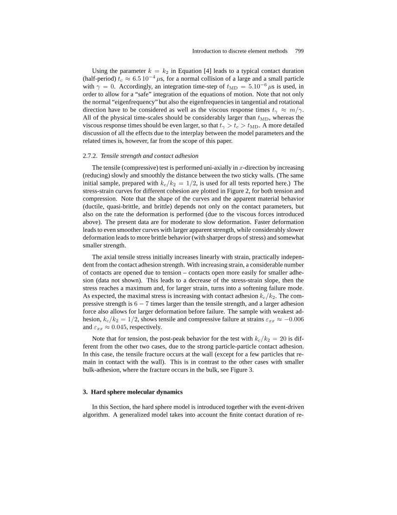
The tensile (compressive) test is performed uni-axially inx-direction by increasing(reducing) slowly and smoothly the distance between the twosticky walls. (The sameinitial sample, prepared withkc/k2 = 1/2, is used for all tests reported here.) Thestress-strain curves for different cohesion are plotted inFigure 2, for both tension andcompression. Note that the shape of the curves and the apparent material behavior(ductile, quasi-brittle, and brittle) depends not only on the contact parameters, butalso on the rate the deformation is performed (due to the viscous forces introducedabove). The present data are for moderate to slow deformation. Faster deformationleads to even smoother curves with larger apparent strength, while considerably slowerdeformation leads to more brittle behavior (with sharper drops of stress) and somewhatsmaller strength.
The axial tensile stress initially increases linearly withstrain, practically indepen-dent from the contact adhesion strength. With increasing strain, a considerable numberof contacts are opened due to tension – contacts open more easily for smaller adhe-sion (data not shown). This leads to a decrease of the stress-strain slope, then thestress reaches a maximum and, for larger strain, turns into asoftening failure mode.As expected, the maximal stress is increasing with contact adhesionkc/k2. The com-pressive strength is6 − 7 times larger than the tensile strength, and a larger adhesionforce also allows for larger deformation before failure. The sample with weakest ad-hesion,kc/k2 = 1/2, shows tensile and compressive failure at strainsεxx ≈ −0.006andεxx ≈ 0.045, respectively.
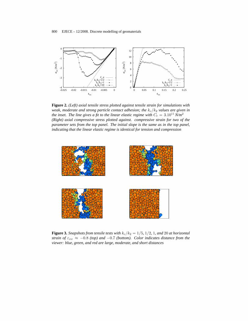
Note that for tension, the post-peak behavior for the test with kc/k2 = 20 is dif-ferent from the other two cases, due to the strong particle-particle contact adhesion.In this case, the tensile fracture occurs at the wall (exceptfor a few particles that re-main in contact with the wall). This is in contrast to the other cases with smallerbulk-adhesion, where the fracture occurs in the bulk, see Figure 3.
3. Hard sphere molecular dynamics
In this Section, the hard sphere model is introduced together with the event-drivenalgorithm. A generalized model takes into account the finitecontact duration of re-
800 EJECE – 12/2008. Discrete modelling of geomaterials
-4
-3
-2
-1
0
-0.025 -0.02 -0.015 -0.01 -0.005 0
σ xx
[N/m
2 ]
εxx
Ct εkc/k2=1/2
kc/k2=1kc/k2=20
12
10
8
6
4
2
0 0 0.05 0.1 0.15 0.2 0.25
σ xx
[N/m
2 ]
εxx
Ct εkc/k2=1/2
kc/k2=1
Figure 2. (Left) axial tensile stress plotted against tensile strainfor simulations withweak, moderate and strong particle contact adhesion; thekc/k2 values are given inthe inset. The line gives a fit to the linear elastic regime with Ct = 3.1011 N/m2
(Right) axial compressive stress plotted against. compressive strain for two of theparameter sets from the top panel. The initial slope is the same as in the top panel,indicating that the linear elastic regime is identical for tension and compression
Figure 3. Snapshots from tensile tests withkc/k2 = 1/5, 1/2, 1, and20 at horizontalstrain of εxx ≈ −0.8 (top) and−0.7 (bottom). Color indicates distance from theviewer: blue, green, and red are large, moderate, and short distances

Introduction to discrete element methods 801
alistic particles and, besides providing a physcial parameter, saves computing timebecause it avoids the “inelastic collapse”.
In the framework of the hard sphere model, particles are assumed to be perfectlyrigid and they follow an undisturbed motion until a collision occurs as described be-low. Due to the rigidity of the interaction, the collisions occur instantaneously, so thatan event-driven simulation method (Lubachevsky, 1991; Luding et al., 1998b; Milleret al., 2004b; Milleret al., 2004a; Miller, 2004) can be used. Note that the ED methodwas only recently implemented in parallel (Lubachevsky, 1992; Miller et al., 2004b);however, we avoid to discuss this issue in detail.
The instantaneous nature of hard sphere collisions is artificial, however, it is avalid limit in many circumstances. Even though details of the contact- or collisionbehavior of two particles are ignored, the hard sphere modelis valid when binary col-lisions dominate and multi-particle contacts are rare (Luding et al., 2003). The lackof physical information in the model allows a much simpler treatment of collisionsthan described in Section 2 by just using a collision matrix based on momentum con-servation and energy loss rules. For the sake of simplicity,we restrict ourselves tosmooth hard spheres here. Collision rules for rough spheresare extensively discussedelsewhere, seee.g.(Ludinget al., 1998a; Herbstet al., 2004), and references therein.
3.1. Smooth hard sphere collision model
Between collisions, hard spheres fly independently from each other. A changein velocity – and thus a change in energy – can occur only at a collision. The stan-dard interaction model for instantaneous collisions of identical particles with radiusa, and massm, is used in the following. The post-collisional velocitiesv′ of twocollision partners in their center of mass reference frame are given, in terms of thepre-collisional velocitiesv, by
v′
1,2 = v1,2 ∓ (1 + r)vn /2 [24]
with vn ≡ [(v1 − v2) · n] n, the normal component of the relative velocityv1 − v2,parallel ton, the unit vector pointing along the line connecting the centers of thecolliding particles. If two particles collide, their velocities are changed accordingto Equation [24], with the change of the translational energy at a collision∆E =−m12(1 − r2)v2
n/2, with dissipation for restitution coefficientsr < 1.
3.2. Event-Driven (ED) algorithm
Since we are interested in the behavior of granular particles, possibly evolving overseveral decades in time, we use an event-driven (ED) method which discretizes thesequence of events with a variable time step adapted to the problem. This is differentfrom classical DEM simulations, where the time step is usually fixed.

802 EJECE – 12/2008. Discrete modelling of geomaterials
In the ED simulations, the particles follow an undisturbed translational motionuntil an event occurs. An event is either the collision of twoparticles or the collision ofone particle with a boundary of a cell (in the linked-cell structure) (Allenet al., 1987).The cells have no effect on the particle motion here; they were solely introduced toaccelerate the search for future collision partners in the algorithm.
Simple ED algorithms update the whole system after each event, a method which isstraightforward, but inefficient for large numbers of particles. In (Lubachevsky, 1991)an ED algorithm was introduced which updates only those two particles involved inthe last collision. Because this algorithm is “asynchronous” in so far that an event,i.e.the nextevent, can occur anywhere in the system, it is so complicatedto parallelizeit (Miller et al., 2004b). For the serial algorithm, a double buffering data structure isimplemented, which contains the ‘old’ status and the ‘new’ status, each consisting of:time of event, positions, velocities, and event partners. When a collision occurs, the‘old’ and ‘new’ status of the participating particles are exchanged. Thus, the former‘new’ status becomes the actual ‘old’ one, while the former ‘old’ status becomes the‘new’ one and is then free for the calculation and storage of possible future events.This seemingly complicated exchange of information is carried out extremely simplyand fast by only exchanging the pointers to the ‘new’ and ‘old’ status respectively.Note that the ‘old’ status of particlei has to be kept in memory, in order to updatethe time of the next contact,tij , of particle i with any other objectj if the latter,independently, changed its status due to a collision with yet another particle. Duringthe simulation such updates may be neccessary several timesso that the predicted‘new’ status has to be modified.
The minimum of alltij is stored in the ‘new’ status of particlei, together withthe corresponding partnerj. Depending on the implementation, positions and ve-locities after the collision can also be calculated. This would be a waste of com-puter time, since before the timetij , the predicted partnersi andj might be involvedin several collisions with other particles, so that we applya delayed update scheme(Lubachevsky, 1991). The minimum times of event,i.e. the times, which indicate thenext event for a certain particle, are stored in an ordered heap tree, such that the nextevent is found at the top of the heap with a computational effort of O(1); changingthe position of one particle in the tree from the top to a new position needsO(logN)operations. The search for possible collision partners is accelerated by the use ofa standard linked-cell data structure and consumesO(1) of numerical resources perparticle. In total, this results in a numerical effort ofO(N logN) for N particles.For a detailed description of the algorithm see (Lubachevsky, 1991). Using all thesealgorithmic tricks, we are able to simulate about105 particles within reasonable timeon a low-end PC (Ludinget al., 1999), where the particle number is more limited bymemory than by CPU power. Parallelization, however, is a means to overcome thelimits of one processor (Milleret al., 2004b).
As a final remark concerning ED, one should note that the disadvantages con-ncected to the assumptions made that allow to use an event driven algorithm limit theapplicability of this method. Within their range of applicability, ED simulations are

Introduction to discrete element methods 803
typically much faster than DEM simulations, since the former accounts for a collisionin one basic operation (collision matrix), whereas the latter requires about one hundredbasic steps (integration time steps). Note that this statement is also true in the denseregime. In the dilute regime, both methods give equivalent results, because collisionsare mostly binary (Ludinget al., 1994a). When the system becomes denser, multi-particle collisions can occur and the rigidity assumption within the ED hard sphereapproach becomes invalid.
The most striking difference between hard and soft spheres is the fact that softparticles dissipate less energy when they are in contact with many others of their kind.In the following chapter, the so called TC model is discussedas a means to accountfor the contact durationtc in the hard sphere model.
4. The link between ED and DEM with the TC model
In the ED method the contact duration is implicitly zero, matching well thecorresponding assumption of instantaneous contacts used for the kinetic theory(Haff, 1983; Jenkinset al., 1985). Due to this artificial simplification (which disre-gards the fact that a real contact takes always finite time) EDalgorithms run into prob-lems when the time between eventstn gets too small: In dense systems with strongdissipation,tn may even tend towards zero. As a consequence the so-called “inelas-tic collapse” can occur,i.e. the divergence of the number of events per unit time.The problem of the inelastic collapse (McNamaraet al., 1994) can be avoided usingrestitution coefficients dependent on the time elapsed since the last event (Ludingetal., 1998b; Ludinget al., 2003). For the contact that occurs at timetij between parti-clesi andj, one usesr = 1 if at least one of the partners involved had a collision withanother particle later thantij − tc. The timetc can be seen as a typical duration of acontact, and allows for the definition of the dimensionless ratio
τc = tc/tn . [25]
The effect oftc on the simulation results is negligible for larger and smalltc; fora more detailed discussion see (Ludinget al., 1998b; Ludinget al., 1999; Ludingetal., 2003).
In assemblies of soft particles, multi-particle contacts are possible and the inelasticcollapse is avoided. The TC model can be seen as a means to allow for multi-particlecollisions in dense systems (Ludinget al., 1996; Luding, 1997; Ludinget al., 1998b).In the case of a homogeneous cooling system (HCS), one can explicitly compute thecorrected cooling rate (r.h.s.) in the energy balance equation
d
dτE = −2I(E, tc) [26]
with the dimensionless timeτ = (2/3)At/tE(0) for 3D systems, scaled byA = (1−r2)/4, and the collision ratet−1
E = (12/a)νg(ν)√
T/(πm), with T = 2K/(3N). In

804 EJECE – 12/2008. Discrete modelling of geomaterials
these units, the energy dissipation rateI is a function of the dimensionless energyE =K/K(0) with the kinetic energyK, and the cut-off timetc. In this representation, therestitution coefficient is hidden in the rescaled time inA = A(r), so that inelastichard sphere simulations with differentr scale on the same master-curve. When theclassical dissipation rateE3/2 (Haff, 1983) is extracted fromI, so thatI(E, tc) =J(E, tc)E
3/2, one has the correction-functionJ → 1 for tc → 0. The deviation fromthe classical HCS is (Ludinget al., 2003):
J(E, tc) = exp (Ψ(x)) [27]
with the series expansionΨ(x) = −1.268x + 0.01682x2 − 0.0005783x3 + O(x4)in the collision integral, withx =
√πtct
−1E (0)
√E =
√πτc(0)
√E =
√πτc (Luding
et al., 2003). This is close to the resultΨLM = −2x/√π, proposed by Luding and
McNamara, based on probabilistic mean-field arguments (Luding et al., 1998b)3.
Given the differential equation [26] and the correction dueto multi-particle con-tacts from Equation [27], it is possible to obtain the solution numerically, and to com-pare it to the classicalEτ = (1 + τ)−2 solution. Simulation results are compared tothe theory in the left panel of Figure 4. The agreement between simulations and the-ory is almost perfect in the examined range oftc-values, only when deviations fromhomogeneity are evidenced one expects disagreement between simulation and theory.The fixed cut-off timetc has no effect when the time between collisions is very largetE ≫ tc, but strongly reduces dissipation when the collisions occur with high fre-quencyt−1
E>∼ t−1
c . Thus, in the homogeneous cooling state, there is a strong effectinitially, and if tc is large, but the long time behavior tends towards the classical decayE → Eτ ∝ τ−2.
The final check if the ED results obtained using the TC model are reasonable is tocompare them to DEM simulations, see the right panel in Figure 4. Open and solidsymbols correspond to soft and hard sphere simulations respectively. The qualitativebehavior (the deviation from the classical HCS solution) isidentical: The energy decayis delayed due to multi-particle collisions, but later the classical solution is recovered.A quantitative comparison shows that the deviation ofE fromEτ is larger for ED thanfor DEM, given that the sametc is used. This weaker dissipation can be understoodfrom the strict rule used for ED: Dissipation is inactive if any particle had a contactalready. The disagreement between ED and DEM is systematic and should disappearif an about 30 per-cent smallertc value is used for ED. The disagreement is alsoplausible, since the TC model disregards all dissipation for multi-particle contacts,while the soft particles still dissipate energy – even though much less – in the case ofmulti-particle contacts.
The above simulations show that the TC model is in fact a “trick” to make hardparticles soft and thus connecting between the two types of simulation models: softand hard. The only change made to traditional ED involves a reduced dissipation for(rapid) multi-particle contacts.
3. ΨLM thus neglects non-linear terms and underestimates the linear part.

Introduction to discrete element methods 805
1
10
100
1000
0.01 0.1 1 10 100 1000
E/E
τ
τ
τc=2.4τc=1.2τc=0.60τc=0.24τc=1.2 10-2
τc=1.2 10-4
0.98
1
1.02
1.04
1.06
1.08
1.1
1.12
1.14
1.16
0.01 0.1 1 10 100
E/E
τ
τ
tc=10-2
tc=5.10-3
tc=10-3
Figure 4. (Left) deviation from the HCS, i.e. rescaled energyE/Eτ , whereEτ is theclassical solutionEτ = (1 + τ)−2. The data are plotted againstτ for simulationswith differentτc(0) = tc/tE(0) as given in the inset, withr = 0.99, andN = 8000.Symbols are ED simulation results, the solid line results from the third order correc-tion. (Right)E/Eτ plotted againstτ for simulations withr = 0.99, andN = 2197.Solid symbols are ED simulations, open symbols are DEM (softparticle simulations)with three differenttc as given in the inset
5. The stress in particle simulations
The stress tensor is a macroscopic quantity that can be obtained by measurementof forces per area, or by a so-called micro-macro homogenization procedure. Bothmethods will be discussed below. During derivation, it alsoturns out that stress hastwo contributions, the first is the “static stress” due to particle contacts, apotentialenergy density, the second is the “dynamics stress” due to momentum flux, like in theideal gas, akinetic energy density. For the sake of simplicity, we restrict ourselves tothe case of smooth spheres here.
5.1. Dynamic stress
For dynamic systems, one has momentum transport in form of flux of the particles.This simplest contribution to the stress tensor is the standard stress in an ideal gas,where the atoms (mass points) move with a certain fluctuationvelocityvi. The kineticenergyE =
∑Ni=1mv
2i /2 due to the fluctuation velocityvi can be used to define the
temperature of the gaskBT = 2E/(DN), with the dimensionD and the particlenumberN . Given a number densityn = N/V , the stress in the ideal gas is thenisotropic and thus quantified by the pressurep = nkBT ; note that we will disregardkB in the following. In the general case, the dynamic stress isσ = (1/V )
∑
i mi vi⊗vi, with the dyadic tensor product denoted by ‘⊗’, and the pressurep = trσ/D = nTis the kinetic energy density.

806 EJECE – 12/2008. Discrete modelling of geomaterials
The additional contribution to the stress is due to collisions and contacts and willbe derived from the principle of virtual displacement for soft interaction potentialsbelow, and then be modified for hard sphere systems.
5.2. Static stress from virtual displacements
From the centers of massr1 andr2 of two particles, we define the so-called branchvector l = r1 − r2, with the reference distancel = |l| = 2a at contact, and thecorresponding unit vectorn = l/l. The deformation in the normal direction, relativeto the reference configuration, is defined asδ = 2an − l. A virtual change of thedeformation is then
∂δ = δ′ − δ ≈ ∂l = ε · l [28]
where the prime denotes the deformation after the virtual displacement described bythe tensorε. The corresponding potential energy density due to the contacts of onepair of particles isu = kδ2/(2V ), expanded to second order inδ, leading to thevirtual change
∂u =k
V
(
δ · ∂δ +1
2(∂δ)2
)
≈ k
Vδ · ∂ln [29]
wherek is the spring stiffness (the prefactor of the quadratic termin the series expan-sion of the interaction potential),V is the averaging volume, and∂ln = n(n · ε · l) isthe normal component of∂l. Note that∂u depends only on the normal component of∂δ due to the scalar product withδ, which is parallel ton.
From the potential energy density, we obtain the stress froma virtual deformationby differentiation with respect to the deformation tensor components
σ =∂u
∂ε=k
Vδ ⊗ l =
1
Vf ⊗ l [30]
wheref = kδ is the force acting at the contact, and the dyadic product⊗ of twovectors leads to a tensor of rank two.
5.3. Stress for soft and hard spheres
Combining the dynamic and the static contributions to the stress tensor (Ludingetal., 2001c), one has for smooth, soft spheres:
σ =1
V
[
∑
i
mivi ⊗ vi −∑
c∈V
fc ⊗ lc
]
[31]
Introduction to discrete element methods 807
where the right sum runs over all contactsc in the averaging volumeV . Replacing theforce vector by momentum change per unit time, one obtains for hard spheres:
σ =1
V
∑
i
mivi ⊗ vi −1
∆t
∑
n
∑
j
pj ⊗ lj
[32]
wherepj andlj are the momentum change and the center-contact vector of particle jat collisionn, respectively. The sum in the left term runs over all particlesi, the firstsum in the right term runs over all collisionsn occurring in the averaging time∆t, andthe second sum in the right term concerns the collision partners of collisionn (Ludinget al., 1998b).
Exemplary stress computations from DEM and ED simulations are presented inthe following Section.
6. Two-dimensional simulation results
Stress computations from two dimensional DEM and ED simulations are presentedin the following subsections. First, a global equation of state, valid for all densities, isproposed based on ED simulations, and second, the stress tensor from a slow, quasi-static deformation is computed from DEM simulations with frictional particles.
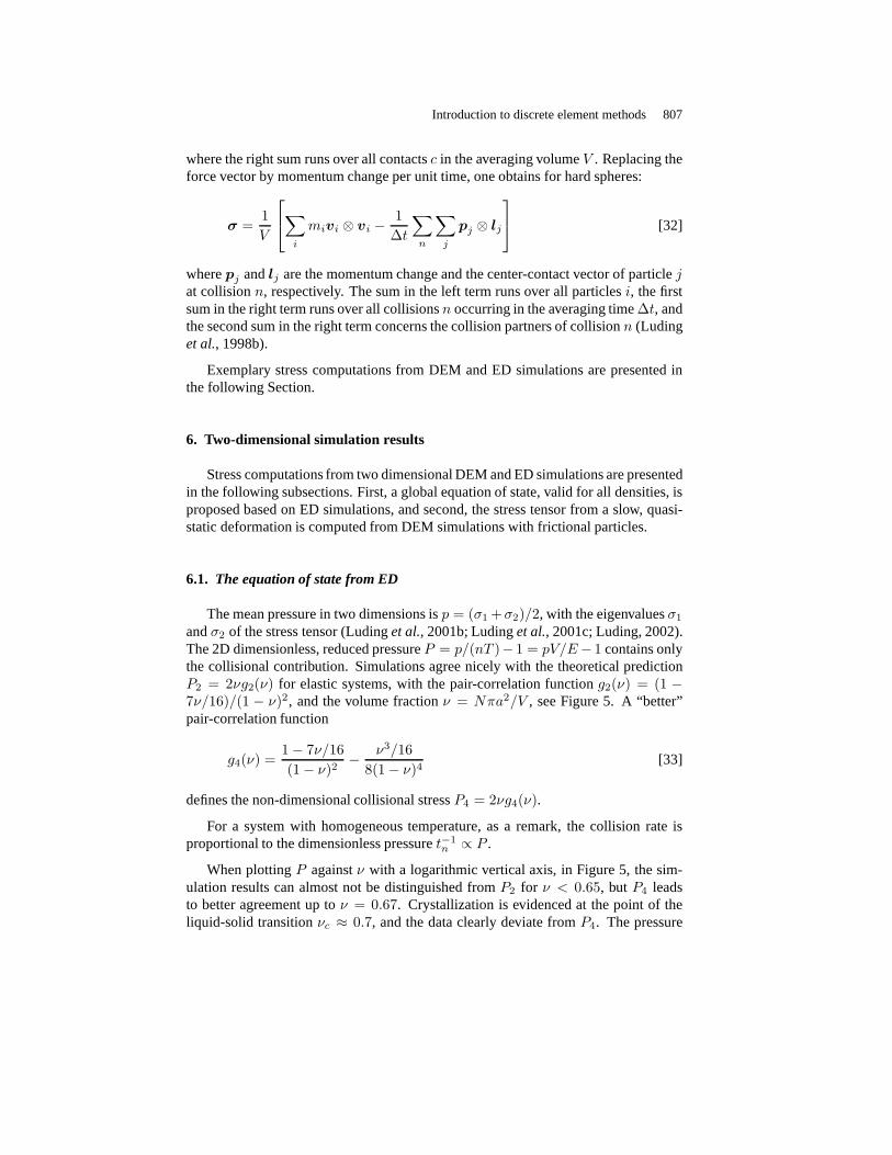
6.1. The equation of state from ED
The mean pressure in two dimensions isp = (σ1 +σ2)/2, with the eigenvaluesσ1
andσ2 of the stress tensor (Ludinget al., 2001b; Ludinget al., 2001c; Luding, 2002).The 2D dimensionless, reduced pressureP = p/(nT )− 1 = pV/E− 1 contains onlythe collisional contribution. Simulations agree nicely with the theoretical predictionP2 = 2νg2(ν) for elastic systems, with the pair-correlation functiong2(ν) = (1 −7ν/16)/(1 − ν)2, and the volume fractionν = Nπa2/V , see Figure 5. A “better”pair-correlation function
g4(ν) =1 − 7ν/16
(1 − ν)2− ν3/16
8(1 − ν)4[33]
defines the non-dimensional collisional stressP4 = 2νg4(ν).
For a system with homogeneous temperature, as a remark, the collision rate isproportional to the dimensionless pressuret−1
n ∝ P .
When plottingP againstν with a logarithmic vertical axis, in Figure 5, the sim-ulation results can almost not be distinguished fromP2 for ν < 0.65, butP4 leadsto better agreement up toν = 0.67. Crystallization is evidenced at the point of theliquid-solid transitionνc ≈ 0.7, and the data clearly deviate fromP4. The pressure

808 EJECE – 12/2008. Discrete modelling of geomaterials
1
10
100
0 0.2 0.4 0.6 0.8
P
ν
QQ0P4
Pdense
8
9
10
0.68 0.7 0.72
Figure 5. The dashed lines areP4 andPdense as functions of the volume fractionν,and the symbols are simulation data, with standard deviations as given by the errorbars in the inset. The thick solid line isQ, the corrected global equation of state fromEquation [34], and the thin solid line isQ0 without empirical corrections
is strongly reduced due to the increase of free volume causedby ordering. Eventu-ally, the data diverge at the maximum packing fractionνmax = π/(2
√3) for a perfect
triangular array.
For high densities, one can compute from free-volume models, the reduced pres-surePfv = 2νmax/(νmax − ν). Slightly different functional forms do not lead tomuch better agreement (Luding, 2002). Based on the numerical data, we propose thecorrected high density pressurePdense = Pfvh(νmax − ν) − 1, with the empirical fitfunctionh(x) = 1+c1x+c3x
3, andc1 = −0.04 andc3 = 3.25, in perfect agreementwith the simulation results forν ≥ 0.73.
Since, to our knowledge, there is no conclusive theory available to combine thedisordered and the ordered regime (Kawamura, 1979), we propose a global equationof state
Q = P4 +m(ν)[Pdense − P4] [34]
with an empirical merging functionm(ν) = [1 + exp (−(ν − νc)/m0)]−1, which
selectsP4 for ν ≪ νc andPdense for ν ≫ νc, with the transition densityνc and thewidth of the transitionm0. In Figure 5, the fit parametersνc = 0.702 andm0 ≈0.0062 lead to qualitative and quantitative agreement betweenQ (thick line) and thesimulation results (symbols). However, a simpler versionQ0 = P2 +m(ν)[Pfv −P2],(thin line) without empirical corrections leads already toreasonable agreement whenνc = 0.698 andm0 = 0.0125 are used. In the transition region, this functionQ0

Introduction to discrete element methods 809
has no negative slope but is continuous and differentiable,so that it allows for aneasy and compact numerical integration ofP . We selected the parameters forQ0 asa compromise between the quality of the fit on the one hand and the simplicity andtreatability of the function on the other hand.
As an application of the global equation of state, the density profile of a densegranular gas in the gravitational field has been computed formonodisperse (Ludingetal., 2001c) and bidisperse situations (Ludinget al., 2001b; Luding, 2002). In the lattercase, however, segregation was observed and the mixture theory could not be applied.The equation of state and also other transport properties are extensively discussed in(Alam et al., 2002b; Alamet al., 2002a; Alamet al., 2003b; Alamet al., 2003a) for2D, bi-disperse systems.
6.2. Quasi-static DEM simulations
In contrast to the dynamic, collisional situation discussed in the previous Section,a quasi-static situation, with all particles almost at restmost of the time, is discussedin the following.
6.2.1. Model parameters
The systems examined in the following containN = 1950 particles with radiiai
randomly drawn from a homogeneous distribution with minimum amin = 0.5 10−3 mand maximumamax = 1.5 10−3 m. The massesmi = (4/3)ρπa3
i , with the densityρ = 2.0 103 kg m−3, are computed as if the particles were spheres. This is an artificialchoice and introduces some dispersity in mass in addition tothe dispersity in size.Since we are mainly concerned about slow deformation and equilibrium situations,the choice for the calculation of mass should not matter. Thetotal mass of the particlesin the system is thusM ≈ 0.02 kg with the typical reduced mass of a pair of particleswith mean radius,m12 ≈ 0.42 10−5 kg. If not explicitly mentioned, the materialparameters arek2 = 105 N m−1 andγ0 = 0.1 kg s−1. The other spring-constantsk1
andkc will be defined in units ofk2. In order to switch on adhesion,k1 < k2 andkc > 0 is used; if not mentioned explicitly,k1 = k2/2 is used, andk2 is constant,independent of the maximum overlap previously achieved.
Using the parametersk1 = k2 and kc = 0 in Equation [4] leads to a typicalcontact duration (half-period):tc ≈ 2.03 10−5 s for γ0 = 0, tc ≈ 2.04 10−5 s forγ0 = 0.1 kg s−1, andtc ≈ 2.21 10−5 s for γ0 = 0.5 kg s−1 for a collision. Accord-ingly, an integration time-step oftDEM = 5 10−7 s is used, in order to allow for a‘safe’ integration of contacts involving smaller particles. Large values ofkc lead tostrong adhesive forces, so that also more energy can be dissipated in one collision.The typical response time of the particle pairs, however, isnot affected so that thenumerical integration works well from a stability and accuracy point of view.

810 EJECE – 12/2008. Discrete modelling of geomaterials
6.2.2. Boundary conditions
The experiment chosen is the bi-axial box set-up, see Figure6, where the leftand bottom walls are fixed, and stress- or strain-controlleddeformation is applied.In the first case a wall is subject to a predefined pressure, in the second case, thewall is subject to a pre-defined strain. In a typical ‘experiment’, the top wall is straincontrolled and slowly shifted downwards while the right wall moves stress controlled,dependent on the forces exerted on it by the material in the box. The strain-controlledposition of the top wall as function of timet is here
z(t) = zf +z0 − zf
2(1 + cosωt) , with εzz = 1 − z
z0[35]
where the initial and the final positionsz0 andzf can be specified together with therate of deformationω = 2πf so that after a half-periodT/2 = 1/(2f) the extremaldeformation is reached. With other words, the cosine is active for 0 ≤ ωt ≤ π. Forlarger times, the top-wall is fixed and the system can relax indefinitely. The cosinefunction is chosen in order to allow for a smooth start-up andfinish of the motionso that shocks and inertia effects are reduced, however, theshape of the function isarbitrary as long as it is smooth.
ε
px
x
z zz
tz(
T
)
z
z0
f
t0 /2
Figure 6. (Left) schematic drawing of the model system. (Right) position of the top-wall as function of time for the strain-controlled situation
The stress-controlled motion of the side-wall is describedby
mwx(t) = Fx(t) − pxz(t) − γwx(t) [36]
wheremw is the mass of the right side wall. Large values ofmw lead to slow adaption,small values allow for a rapid adaption to the actual situation. Three forces are active:(i) the forceFx(t) due to the bulk material, (ii) the force−pxz(t) due to the externalpressure, and (iii) a strong frictional force which damps the motion of the wall so thatoscillations are reduced.
Introduction to discrete element methods 811
6.2.3. Initial configuration and compression
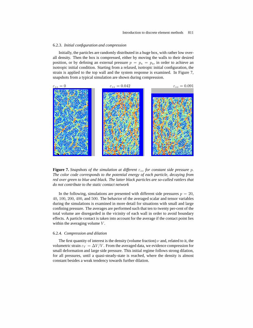
Initially, the particles are randomly distributed in a hugebox, with rather low over-all density. Then the box is compressed, either by moving thewalls to their desiredposition, or by defining an external pressurep = px = pz, in order to achieve anisotropic initial condition. Starting from a relaxed, isotropic initial configuration, thestrain is applied to the top wall and the system response is examined. In Figure 7,snapshots from a typical simulation are shown during compression.
εzz = 0 εzz = 0.042 εzz = 0.091
Figure 7. Snapshots of the simulation at differentεzz for constant side pressurep.The color code corresponds to the potential energy of each particle, decaying fromred over green to blue and black. The latter black particles are so-called rattlers thatdo not contribute to the static contact network
In the following, simulations are presented with differentside pressuresp = 20,40, 100, 200, 400, and500. The behavior of the averaged scalar and tensor variablesduring the simulations is examined in more detail for situations with small and largeconfining pressure. The averages are performed such that tento twenty per-cent of thetotal volume are disregarded in the vicinity of each wall in order to avoid boundaryeffects. A particle contact is taken into account for the average if the contact point lieswithin the averaging volumeV .
6.2.4. Compression and dilation
The first quantity of interest is the density (volume fraction)ν and, related to it, thevolumetric strainεV = ∆V/V . From the averaged data, we evidence compression forsmall deformation and large side pressure. This initial regime follows strong dilation,for all pressures, until a quasi-steady-state is reached, where the density is almostconstant besides a weak tendency towards further dilation.

812 EJECE – 12/2008. Discrete modelling of geomaterials
0.82
0.83
0.84
0.85
0.86
0.87
0 0.05 0.1 0.15 0.2
ν
εzz
p=500p=400p=200p=100p=20
-0.01
0
0.01
0.02
0.03
0 0.05 0.1 0.15 0.2
ε V
εzz
p=20p=40
p=100p=200p=400p=500
Figure 8. (Left) volume fractionν =∑
i πa2i /V for different confining pressurep.
(Right) volumetric strain – negative values mean compression, whereas positive valuescorrespond to dilation
An initially dilute granular medium (weak confining pressure) thus shows dilationfrom the beginning, whereas a denser granular material (strong confining pressure)can be compressed even further by the relatively strong external forces until dilationstarts. The range of density changes is about 0.02 in volume fraction and spans up to3 % changes in volumetric strain.
From the initial slope, one can obtain the Poisson ratio of the bulk material, andfrom the slope in the dilatant regime, one obtains the so-called dilatancy angle, ameasure of the magnitude of dilatancy required before shearis possible (Ludingetal., 2001a; Luding, 2004a).
6.2.5. Fabric tensor
The fabric tensor is computed according to (Luding, 2005b; Luding, 2005a), andits isotropic and deviatoric contributions are displayed in Figure 9. The isotropiccontribution (the contact number density) is scaled by the prediction from (Madadiet al., 2004), and the deviation from the prediction is between oneto three percent,where the larger side pressure data are in better agreement (smaller deviation). Notethat the correction due to the factorg2 corresponds to about nine per-cent, and that thedata are taken in the presence of friction, in contrast to thesimulations by (Madadietal., 2004), a source of discrepancy, which accounts in our opinion for the remainingdeviation.
The anisotropy of the granular packing is quantified by the deviatoric fabric, asdisplayed in its scaled form in Figure 9. The anisotropy is initially of the order of afew percent at most – thus the initial configurations are not perfectly isotropic. Withincreasing deviatoric deformation, the anisotropy grows,reaches a maximum and then

Introduction to discrete element methods 813
0.96
0.98
1
1.02
1.04
1.06
0 0.02 0.04 0.06 0.08 0.1 0.12 0.14
tr F
/ (g
2ν C
)
εzz
p=20p=40
p=100p=200p=400p=500
0
0.05
0.1
0.15
0.2
0 0.025 0.05 0.075 0.1
dev
F /
tr F
εD
p=20p=40
p=100p=200p=400p=500
Figure 9. (Left) quality factor for the trace of the fabric tensor scaled by the analyticalpredictiong2νC from (Madadiet al., 2004), for different pressuresp, as function ofthe vertical deformation. (Right) deviatoric fraction of the fabric tensor from the samesimulations plotted against the deviatoric strain
saturates on a lower level in the critical state flow regime. The scaled fabric growsfaster for smaller side pressure and is also relatively larger for smallerp. The non-scaled fabric deviator, astonishingly, grows to values aroundfmax
D trF ≈ 0.56± 0.03,independently of the side pressures used here (data not shown, see (Luding, 2004a;Luding, 2004b) for details). Using the definitionfD := devF /trF , the functionalbehavior,
∂fD
∂εD= βf (fmax
D − fD) [37]
was evidenced from simulations in (Luding, 2004a), withfmaxD trF ≈ const., and the
deviatoric rate of approachβf = βf (p), decreasing with increasing side pressure. Thedifferential equation is solved by an exponential functionthat describes the approachof the anisotropyfD to its maximal value,1 − (fD/f
maxD ) = exp (−βfεD), but not
beyond.
6.2.6. Stress tensor
The sums of the normal and the tangential stress-contributions are displayed inFigure 10 for two side-pressuresp = 20 andp = 200. The lines show the stressmeasured on the walls, and the symbols correspond to the stress measured with themicro-macro average in Equation [31], proving the reasonable quality of the micro-macro transition as compared to the wall stress “measurement”.
There is also other macroscopic information hidden in the stress-strain curves inFigure 10. From the initial, rapid increase in stress, one can determine moduli of thebulk-material,i.e, the stiffness under confinementp. Later, the stress reaches a peakat approximately2.6p and then saturates at about2p. From both peak- and saturation

814 EJECE – 12/2008. Discrete modelling of geomaterials
stress, one obtains the yield stresses at peak and in critical state flow, respectively(Schwedes, 2003).
0
20
40
60
80
0 0.05 0.1 0.15 0.2
σn +σt
εzz
p=20
pzpx
σzzσxx
0
200
400
600
800
0 0.05 0.1 0.15 0.2
σn +σt
εzz
p=200
pzpx
σzzσxx
Figure 10. Total stress tensorσ = σn + σt for small (left) and high (right) pressure– the agreement between the wall pressure and the averaged stress is almost perfect
Note that for the parameters used here, both the dynamic stress and the tangentialcontributions to the stress tensor are more than one order ofmagnitude smaller thanthe normal contributions. As a cautionary note, we remark also that the artificial stressinduced by the background viscous force is negligible here (about two per-cent), whenγb = 10−3 kg s−1 and a compression frequencyf = 0.1 s−1 are used. For fastercompression withf = 0.5 s−1, one obtains about ten per-cent contribution to stressfrom the artificial background force.
The behavior of the stress is displayed in Figure 11, where the isotropic stress12tr σ is plotted in units ofp, and the deviatoric fraction is plotted in units of the
isotropic stress. Note that the tangential forces do not contribute to the isotropic stresshere since the corresponding entries in the averaging procedure compensate. FromFigure 11, we evidence that both normal contributions, the non-dimensional traceand the non-dimensional deviator behave similarly, independent of the side pressure:Starting from an initial value, a maximum is approached, where the maximum is onlyweakly dependent onp.
The increase of stress is faster for lowerp. After the maximum is reached,the stresses decay and approach a smaller value in the critical state flow regime.Using the definitionssV := trσ/(2p) − 1 and sD := devσ/trσ, the maxi-mal (non-dimensional) isotropic and deviatoric stresses are smax
V ≈ 0.8 ± 0.1 andsmax
D ≈ 0.4 ± 0.02, respectively, with a rather large error margin. The correspondingvalues at critical state flow aresc
V ≈ 0.4 ± 0.1 andscD ≈ 0.29 ± 0.04.

Introduction to discrete element methods 815
0
0.5
1
1.5
2
0 0.02 0.04 0.06 0.08 0.1
tr σ
n / 2p
εzz
p=20p=40
p=100p=200p=400p=500
0
0.1
0.2
0.3
0.4
0 0.05 0.1 0.15 0.2
dev
σn / tr
σn
εD
p=20p=40
p=100p=200p=400p=500
Figure 11. Non-dimensional stress tensor contributions for different p. The isotropic(left) and the deviatoric fractions (right) are displayed as functions of the vertical anddeviatoric strain, respectively
The evolution of thedeviatoric stressfraction,sD, as function ofεD, is displayedin Figure 11. Like the fabric, also the deviatoric stress exponentially approaches itsmaximum. This is described by the differential equation
∂sD
∂εD= βs (smax
D − sD) [38]
whereβs = βs(p) is decaying with increasingp (roughly asβs ≈ p−1/2). For moredetails on the deviatoric stress and also on the tangential contribution to the stress, see(Luding, 2004a; Luding, 2004b; Luding, 2005b; Luding, 2005a).
7. Larger computational examples
In this Section, several examples of rather large particle numbers simulated withDEM and ED are presented. The ED algorithm is first used to simulate a freely coolingdissipative gas in two and three dimensions (Ludinget al., 1999; Milleret al., 2004a).Then, a peculiar three dimensional ring-shear experiment is modeled with soft sphereDEM.
7.1. Free cooling and cluster growth (ED)
In the following, a two-dimensional system of lengthL = l/d = 560 with N =99856 dissipative particles of diameterd = 2a is examined (Ludinget al., 1998b;Luding et al., 1999), with volume fractionν = 0.25 and restitution coefficientr =0.9. This 2D system is compared to a three-dimensional system oflengthL = l/d =

816 EJECE – 12/2008. Discrete modelling of geomaterials
129 withN = 512000 dissipative spheres of diameterd and volume fractionν = 0.25with r = 0.3 (Miller et al., 2004a).
7.1.1. Initial configuration
Initially the particles are arranged on a square lattice with random velocities drawnfrom an interval with constant probability for each coordinate. The mean total veloc-ity, i.e. the random momentum due to the fluctuations, is eliminated inorder to have asystem with its center of mass at rest. The system is allowed to evolve for some time,until the arbitrary initial condition is forgotten,i.e. the density is homogeneous, andthe velocity distribution is a Gaussian in each coordinate.Then dissipation is switchedon and the evolution of the system is reported for the selected r. In order to avoid theinelastic collapse, the TC model is used, which reduces dissipation if the time betweencollisions drops below a value oftc = 10−5 s.
Figure 12. (Left) collision frequency of individual particles from a 2D simulation,after about 5200 collisions per particle. (Right) cluster visualization from a 3D sim-ulation. The colors in both panels indicate large (red), medium (green), and small(blue) collision rates
7.1.2. System evolution
For the values ofr used here, the system becomes inhomogeneous quite rapidly(Ludinget al., 1999; Milleret al., 2004a). Clusters, and thus also dilute regions, buildup and have the tendency to grow. Since the system is finite, their extension will reachsystem size at a finite time. Thus we distinguish between three regimes of systemevolution: (i) the initially (almost) homogeneous state, (ii) the cluster growth regime,and (iii) the system size dependent final stage where the clusters have reached systemsize. We note that a cluster does not behave like a solid body,but has internal motionand can eventually break into pieces after some time. These pieces (small clusters)collide and can merge to larger ones.

Introduction to discrete element methods 817
In Figure 12, snapshots are presented and the collision rateis color-coded. Thecollision rate and the pressure are higher inside the clusters than at their surface. Notethat most of the computational effort is spent in predictingcollisions and to computethe velocities after the collisions. Therefore, the regions with the largest collision fre-quencies require the major part of the computational resources. Due to the TC model,this effort stays limited and the simulations can easily continue for many thousandcollisions per particle.
7.1.3. Discussion
Note that an event driven simulation can be 10-100 times faster than a soft-particleDEM code applied to model the same particle number. However,ED is rather limitedto special, simple interactions between the particles. Further examples of event-drivensimulations will be presented in the paper by T. Pöschel in this book.
7.2. Ring shear cell simulation in 3D
The simulation in this Section models a ring-shear cell experiment, as recentlyproposed (Fenisteinet al., 2003; Fenisteinet al., 2004). The interesting observationin the experiment is a universal shear zone, initiated at thebottom of the cell andbecoming wider and moving inwards while propagating upwards in the system.
In the following, the shear-band will be examined, and the micro-macro transitionfrom will be performed, leading to a yield stress (or flow function) based on a singlesimulation. This is in contrast to the two-dimensional example from the previouschapter, where the yield stress had to be determined from different simulations withdifferent side stressp. In the ring shear cell, space- and time-averaging is possible, sothat - at different radial and vertical positions, one obtains data for different density,stress, velocity gradient, etc.
7.2.1. Model system
The numerical model chosen here is DEM with smooth particlesin three dimen-sions. In order to save computing time, only a quarter of the ring-shaped geometry issimulated. The walls are cylindrical, and are rough on the particle scale due to someattached particles. The outer cylinder wall with radiusRo, and part of the bottomr > Rs are rotating around the symmetry axis, while the inner wall with radiusRi,and the attached bottom-diskr < Rs remain at rest. In order to resemble the exper-iment, the geometry data areRi = 0.0147m, Rs = 0.085m, andRo = 0.110m.Note that the smallRi value is artificial, but it does not affect the results for small andintermediate filling heights.
The slit in the bottom wall atr = Rs triggers a shear band. In order to examine thebehavior of the shear band as function of the filling heightH , this system is filled with6000 to 64000 spherical particles with mean radius1.0 mm and radii range0.5mm< a < 1.5 mm, which interact here with repulsive and dissipative forces only. The

818 EJECE – 12/2008. Discrete modelling of geomaterials
particles are forced towards the bottom by the gravity forcef g = mg here and are keptinside the system by the cylindrical walls. In order to provide some wall roughness, afraction of the particles (about 3 per-cent) that are originally in contact with the wallsare glued to the walls and move with them.
7.2.2. Material and system parameters
The material parameters for the particle-particle and -wall interactions arek =102 N/m andγ0 = 2.10−3 kg/s. Assuming a collision of the largest and the smallestparticle used, the reduced massm12 = 2.94 10−6 kg, leads to a typical contact dura-tion tc = 5.4 10−4 s and a restitution coefficient ofr = 0.83. The integration time stepis tDEM = 5.10−6 s, i.e. two orders of magnitude smaller than the contact duration.
Figure 13. Snapshots from the quarter-cylinder geometry. Visible arehere only thoseparticles glued to the wall; the cylinder and slit positionsare indicated by the lines,top-view (left) and front-view (right). The colors blue andred correspond to static andmoving wall particles
The simulations run for 25 s with a rotation ratefo = 0.01 s−1 of the outer cylin-der, with angular velocityΩo = 2πfo. For the average of the displacement, only timest > 10 s are taken into account. Within the averaging accuracy, thesystem seeminglyhas reached a quasi-steady state after about 8 s. The empty cell is shown in Figure 13,while three realizations with different filling height are displayed in Figure 14, bothas top- and front-view.
7.2.3. Shear deformation results
From the top-view, it is evident that the shear band moves inwards with increasingfilling height, and it also becomes wider. From the front-view, the same informationcan be evidenced and, in addition, the shape of the shear bandinside the bulk is visible:The inwards displacement happens deep in the bulk and the position of the shear bandis not changing a lot closer to the surface.

Introduction to discrete element methods 819
N = 16467 N = 34518 N = 60977
Figure 14. Snapshots from simulations with different filling heights seen from the topand from the front, and the particle numberN is given in the inset. The colors blue,green, orange and red denote particles withrdφ ≤ 0.5 mm,rdφ ≤ 2 mm,rdφ ≤4 mm, andrdφ > 4 mm, i.e. the displacement in tangential direction per second,respectively. The filling heights in these simulations areH = 0.018m, 0.037m, and0.061m (from left to right)
In order to allow for a more quantitative analysis of the shear band, both on the topand as function of depth, we perform fits with the universal shape function proposedin (Fenisteinet al., 2003):
vϕ(r)
rΩo= A
(
1 + erf
(
r −Rc
W
))
[39]
whereA is a dimensionless amplitudeA = 0.50 ± 0.02, Rc is the center of theshearband, andW its width.
The fits to the simulations confirm qualitatively the experimental findings in so farthat the center of the shear band, as observed on top of the material, see Figure 15,moves inwards with aRc ∝ H5/2 behavior, and that the width of the shear band in-creases almost linearly withH . For filling heights larger thanH ≈ 0.05 m, deviationsfrom this behavior are observed, because the inner cylinderis reached and thus sensedby the shearband. Slower shearing does not affect the center, but reduces slightly thewidth - as checked by one simulation.
Like in the experiments, the behavior of the shearband within the bulk, see Figure16, deviates qualitatively from the behavior seen from the top. Instead of a slowmotion of the shear band center inwards, the shear band rapidly moves inwards at

820 EJECE – 12/2008. Discrete modelling of geomaterials
-0.005
0
0.005
0.01
0.015
0.02
0.025
0.03
0.035
0.04
0 0.01 0.02 0.03 0.04 0.05 0.06 0.07
Rs-
Rc
(m)
H (m)
cR H5/2
0
0.005
0.01
0.015
0.02
0.025
0.03
0.035
0.04
0 0.01 0.02 0.03 0.04 0.05 0.06 0.07
W (
m)
H (m)
cW H
Figure 15. (Left) distance of the top-layer shearband center from the slit, both plottedagainst the filling heightH . The open symbols are simulation results, the solid symbolis a simulation with slower rotationfo = 0.005 s−1, and the line is a fit with constantcR = 30. (Right) width of the shearband from the same simulations; the line is a fitwith cW = 2/5
small heightsh, and reaches a saturation distance with small change closerto thesurface. Again, a slower rotation does not affect the centerbut reduces the width.
0
0.005
0.01
0.015
0.02
0.025
0.03
0.035
0.04
0 0.01 0.02 0.03 0.04 0.05 0.06 0.07
Rs-
Rc
(m)
h (m)
cR H05/2
0
0.005
0.01
0.015
0.02
0.025
0.03
0.035
0.04
0 0.01 0.02 0.03 0.04 0.05 0.06 0.07
W (
m)
h (m)
cW H0
Figure 16. (Left) distance of the bulk shearband center from the slit. (Right) widthof the shearband, both plotted against the heighth. The open symbols are simulationresults obtained withfo = 0.01 s−1, the solid symbols are obtained with slower rota-tion fo = 0.005 s−1. Squares, circles and triangles correspond to the filling heightsH = 0.037m, 0.049m, and0.061m, respectively. The curves are identical to thoseplotted in Figure 15

Introduction to discrete element methods 821
From the velocity field in the bulk it is straightforward to compute the velocitygradient tensor and, from this extracting the (symmetric) strain rate:
γ =√
d21 + d2
2 =1
2
√
(
∂vφ
∂r− vφ
r
)2
+
(
∂vφ
∂z
)2
[40]
i.e., the shear intensity in the shear plane (Luding, 2008b). Note that the solid-body rotation termvφ/r comes from the cylindrical coordinate system used. Theshear planes are in fact described by a normal unit vectorγ = (cos θ, 0, sin θ), withθ = θ(r, z) = arccos(d1/γ), as predicted (Depkenet al., 2006). The center of theshear band indicates the direction of the unit-vectorγ. In the system with friction, weobserve that the average particles spin is also normal to theshear-plane,i.e., parallelto γ, within the rather strong fluctuations (data not shown).
From the stress, as computed according to Equation [31], theshear stress is ex-tracted (in analogy to the strain rate) as proposed in (Depken et al., 2006):
|τ | =√
σ2rφ + σ2
zφ . [41]
Remarkably, the shear stress intensity|τ |/p ≈ µ is almost constant for practicallyall averaging volumina with strain rates larger than some threshold value,i.e., γ > γc,with γc ≈ 0.02 s−1. Whether the threshold has a physical meaning or is only anartefact due to the statistical fluctuations in the average data has to be examined furtherby much longer runs with better statistics.
From the constant shear stress intensity in the shear zone, one can determine theMohr-Coulomb-type friction angle of the equivalent macroscopic constitutive law, seeFigure 17, asψ ≈ arcsinµ. Interestingly, without frictionψ is rather large,i.e., muchlarger than expected from a frictionless material, whereasit is astonishingly small withfriction (data not shown),i.e., smaller than the microscopic contact frictionµ = 0.4used, see (Luding, 2008b).
7.2.4. Discussion
In summary, the example of a ring shear cell simulation in 3D has shown, thateven without the more complicated details of fancy interaction laws, experiments canbe reproduced at least qualitatively. A more detailed studyof quantitative agreementhas been performed in 2D (Lätzelet al., 2003), and is in progress for the 3D case.
A challenge for the future remains the micro-macro transition, for which a firstresult has been shown,i.e. the yield stress can be extracted from a single 3D DEMsimulation for various pressures and shear rates. Open remains an objective continuumtheory formulation of the shear band problem.
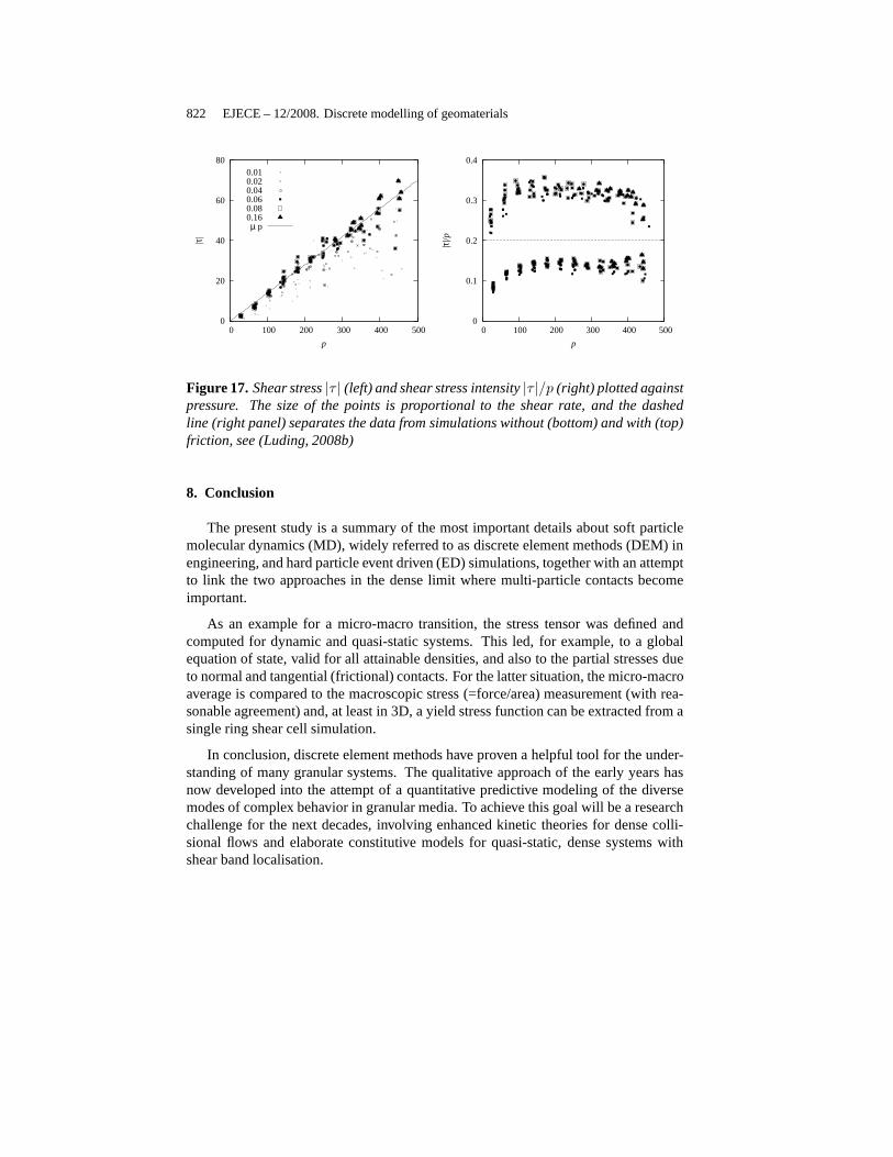
822 EJECE – 12/2008. Discrete modelling of geomaterials
80
60
40
20
0 500 400 300 200 100 0
|τ|
p
0.010.020.040.060.080.16µ p
0.4
0.3
0.2
0.1
0 500 400 300 200 100 0
|τ|/p
p
Figure 17. Shear stress|τ | (left) and shear stress intensity|τ |/p (right) plotted againstpressure. The size of the points is proportional to the shearrate, and the dashedline (right panel) separates the data from simulations without (bottom) and with (top)friction, see (Luding, 2008b)
8. Conclusion
The present study is a summary of the most important details about soft particlemolecular dynamics (MD), widely referred to as discrete element methods (DEM) inengineering, and hard particle event driven (ED) simulations, together with an attemptto link the two approaches in the dense limit where multi-particle contacts becomeimportant.
As an example for a micro-macro transition, the stress tensor was defined andcomputed for dynamic and quasi-static systems. This led, for example, to a globalequation of state, valid for all attainable densities, and also to the partial stresses dueto normal and tangential (frictional) contacts. For the latter situation, the micro-macroaverage is compared to the macroscopic stress (=force/area) measurement (with rea-sonable agreement) and, at least in 3D, a yield stress function can be extracted from asingle ring shear cell simulation.
In conclusion, discrete element methods have proven a helpful tool for the under-standing of many granular systems. The qualitative approach of the early years hasnow developed into the attempt of a quantitative predictivemodeling of the diversemodes of complex behavior in granular media. To achieve thisgoal will be a researchchallenge for the next decades, involving enhanced kinetictheories for dense colli-sional flows and elaborate constitutive models for quasi-static, dense systems withshear band localisation.

Introduction to discrete element methods 823
Acknowledgements
We acknowledge the financial support of several funding institutions that sup-ported the reviewed research, and also the helpful discussions with, and contributionsfrom the many persons that contributed to these results.
9. References
Alam M., Luding S., “ How good is the equipartition assumption for transport properties of agranular mixture”,Granular Matter, vol. 4, n˚ 3, p. 139-142, 2002a.
Alam M., Luding S., “ First normal stress difference and crystallization in a dense shearedgranular fluid”,Phys. Fluids, vol. 15, n˚ 8, p. 2298-2312, 2003a.
Alam M., Luding S., “ Rheology of Bidisperse Granular Mixtures via Event Driven Simula-tions”, J. Fluid Mech., vol. 476, p. 69-103, 2003b.
Alam M., Willits J. T., Arnarson B. O., Luding S., “ Kinetic theory of a binary mixture of nearlyelastic disks with size and mass-disparity”,Physics of Fluids, vol. 14, n˚ 11, p. 4085-4087,2002b.
Allen M. P., Tildesley D. J.,Computer Simulation of Liquids, Oxford University Press, Oxford,1987.
Bartels G., Unger T., Kadau D., Wolf D. E., Kertesz J., “ The effect of contact torques onporosity of cohesive powders”,Granular Matter, vol. 7, p. 139, 2005.
Bashir Y. M., Goddard J. D., “ A novel simulation method for the quasi-static mechanics ofgranular assemblages”,J. Rheol., vol. 35, n˚ 5, p. 849-885, 1991.
Cundall P. A., Strack O. D. L., “ A discrete numerical model for granular assemblies”,Géotech-nique, vol. 29, n˚ 1, p. 47-65, 1979.
David C. T., Garcia-Rojo R., Herrmann H. J., Luding S., “ Powder Flow Testing with 2D and3D Biaxial and Triaxial simulations”,Particle and Particle Systems Characterization, vol.24, n˚ 1, p. 29-33, 2007.
David C. T., Rojo R. G., Herrmann H. J., Luding S., “ Hysteresis and creep in powders andgrains”,in R. Garcia-Rojo, H. J. Herrmann, S. McNamara (eds),Powders and Grains 2005,Balkema, Leiden, Netherlands, p. 291-294, 2005.
Depken M., van Saarloos W., van Hecke M., “ Continuum approach to wide shear zones inquasistatic granular matter”,Phys. Rev. E, vol. 73, p. 031302, 2006.
Dintwa E., van Zeebroeck M., Tijskens E., Ramon H., “ Torsionof viscoelastic spheres incontact”,Granular Matter, vol. 7, p. 169, 2005.
Els D., “ Definition of roll velocity for spherical particles”, 2006, preprint – unpublished.
Fenistein D., van de Meent J. W., van Hecke M., “ Universal andwide shear zones in granularbulk flow”, Phys. Rev. Lett., vol. 92, p. 094301, 2004. e-print cond-mat/0310409.
Fenistein D., van Hecke M., “ Kinematics – Wide shear zones ingranular bulk flow”,Nature,vol. 425, n˚ 6955, p. 256, 2003.
Haff P. K., “ Grain flow as a fluid-mechanical phenomenon”,J. Fluid Mech., vol. 134, p. 401-430, 1983.

824 EJECE – 12/2008. Discrete modelling of geomaterials
Herbst O., Müller P., Otto M., Zippelius A., “ Local Equationof State and Velocity Distributionsof a Driven Granular Gas”,Phys. Rev. E, vol. 70, p. 051313-1-14, 2004. e-print cond-mat/0402104.
Herrmann H. J., “ Intermittency and self-similarity in granular media”,Powders & Grains 97,Balkema, Rotterdam, 1997.
Herrmann H. J., Hovi J.-P., Luding S. (eds),Physics of dry granular media - NATO ASI SeriesE 350, Kluwer Academic Publishers, Dordrecht, 1998.
Hinrichsen H., Wolf D. E.,The Physics of Granular Media, Wiley VCH, Weinheim, Germany,2004.
Janssen H. A., “ Versuche über Getreidedruck in Silozellen”, Zeitschr. d. Vereines deutscherIngenieure, vol. 39, n˚ 35, p. 1045-1049, 1895.
Jenkins J. T., Richman M. W., “ Kinetic theory for plane shearflows of a dense gas of identical,rough, inelastic, circular disks”,Phys. of Fluids, vol. 28, p. 3485-3494, 1985.
Kawamura H., “ A simple theory of hard disk transition”,Prog. Theor. Physics, vol. 61, p. 1584-1596, 1979.
Kirkwood J. G., Buff F. P., Green M. S., “ The statistical mechanical theory of transport pro-cesses”,J. Chem. Phys., vol. 17, n˚ 10, p. 988, 1949.
Kishino Y. (ed.),Powders & Grains 2001, Balkema, Rotterdam, 2001.
Lätzel M., Luding S., Herrmann H. J., “ Macroscopic materialproperties from quasi-static,microscopic simulations of a two-dimensional shear-cell”, Granular Matter, vol. 2, n˚ 3,p. 123-135, 2000. e-print cond-mat/0003180.
Lätzel M., Luding S., Herrmann H. J., Howell D. W., BehringerR. P., “ Comparing simulationand experiment of a 2D granular Couette shear device”,Eur. Phys. J. E, vol. 11, n˚ 4, p. 325-333, 2003.
Lubachevsky B. D., “ How to Simulate Billards and Similar Systems”,J. Comp. Phys., vol. 94,n˚ 2, p. 255, 1991.
Lubachevsky B. D., “ Simulating Billiards: Serially and in Parallel”, Int.J. in Computer Simu-lation, vol. 2, p. 373-411, 1992.
Luding S., “ Surface Waves and Pattern Formation in VibratedGranular Media”,Powders &Grains 97, Balkema, Amsterdam, p. 373-376, 1997.
Luding S., “ Collisions & Contacts between two particles”,in H. J. Herrmann, J.-P. Hovi,S. Luding (eds),Physics of dry granular media - NATO ASI Series E350, Kluwer AcademicPublishers, Dordrecht, p. 285, 1998.
Luding S., “ Liquid-Solid Transition in bi-disperse granulates”,Advances in Complex Systems,vol. 4, n˚ 4, p. 379-388, 2002.
Luding S., “ Micro-Macro Transition for anisotropic, frictional granular packings”,Int. J. Sol.Struct., vol. 41, p. 5821-5836, 2004a.
Luding S., “ Molecular Dynamics Simulations of Granular Materials”, in H. Hinrichsen, D. E.Wolf (eds),The Physics of Granular Media, Wiley VCH, Weinheim, Germany, p. 299-324,2004b.
Luding S., “ Anisotropy in cohesive, frictional granular media”, J. Phys.: Condens. Matter, vol.17, p. S2623-S2640, 2005a.
Luding S., “ Shear flow modeling of cohesive and frictional fine powder”,Powder Technology,vol. 158, p. 45-50, 2005b.

Introduction to discrete element methods 825
Luding S., “ About contact force-laws for cohesive frictional materials in 2D and 3D”,inP. Walzel, S. Linz, C. Krülle, R. Grochowski (eds),Behavior of Granular Media, ShakerVerlag, p. 137-147, 2006. Band 9, Schriftenreihe Mechanische Verfahrenstechnik, ISBN3-8322-5524-9.
Luding S., “ Contact models for very loose granular materials”, in P. Eberhard (ed.),Symposiumon Multiscale Problems in Multibody System Contacts, Springer, p. 135-150, 2007. ISBN978-1-4020-5980-3.
Luding S., “ Cohesive frictional powders: Contact models for tension”,Granular Matter, vol.10, n˚ 4, p. 235-246, 2008a.
Luding S., “ The effect of friction on wide shear bands”,Part. Science and Technology, vol. 26,n˚ 1, p. 33-42, 2008b.
Luding S., Clément E., Blumen A., Rajchenbach J., Duran J., “Anomalous energy dissipationin molecular dynamics simulations of grains: The “detachment effect””, Phys. Rev. E, vol.50, p. 4113, 1994a.
Luding S., Clément E., Blumen A., Rajchenbach J., Duran J., “The onset of convection inMolecular dynamics simulations of grains”,Phys. Rev. E, vol. 50, p. R1762, 1994b.
Luding S., Clément E., Rajchenbach J., Duran J., “ Simulations of Pattern Formation in VibratedGranular Media”,Europhys. Lett., vol. 36, n˚ 4, p. 247-252, 1996.
Luding S., Goldshtein A., “ Collisional cooling with multi-particle interactions”,Granular Mat-ter, vol. 5, n˚ 3, p. 159-163, 2003.
Luding S., Herrmann H. J., “ Cluster growth in freely coolinggranular media”,Chaos, vol. 9,n˚ 3, p. 673-681, 1999.
Luding S., Herrmann H. J., “ Micro-macro transition for cohesive granular media”, 2001a, in:Bericht Nr. II-7, Inst. für Mechanik, Universität Stuttgart, S. Diebels (Ed.).
Luding S., Huthmann M., McNamara S., Zippelius A., “ Homogeneous cooling of rough dissi-pative particles: Theory and simulations”,Phys. Rev. E, vol. 58, p. 3416-3425, 1998a.
Luding S., Lätzel M., Herrmann H. J., “ From discrete elementsimulations towards a continuumdescription of particulate solids”,in A. Levy, H. Kalman (eds),Handbook of Conveying andHandling of Particulate Solids, Elsevier, Amsterdam, The Netherlands, p. 39-44, 2001b.
Luding S., Lätzel M., Volk W., Diebels S., Herrmann H. J., “ From discrete element simulationsto a continuum model”,Comp. Meth. Appl. Mech. Engng., vol. 191, p. 21-28, 2001c.
Luding S., Manetsberger K., Muellers J., “ A discrete model for long time sintering”,Journalof the Mechanics and Physics of Solids, vol. 53(2), p. 455-491, 2005.
Luding S., McNamara S., “ How to handle the inelastic collapse of a dissipative hard-spheregas with the TC model”,Granular Matter, vol. 1, n˚ 3, p. 113-128, 1998b. e-print cond-mat/9810009.
Luding S., Suiker A., “ Self-healing of damaged particulatematerials through sintering”, 2008,Philosophical Magazine, in press.
Luding S., Suiker A., Kadashevich I., “ Discrete element modeling of self-healing processes indamaged particulate materials”,in A. J. M. Schmets, S. van der Zwaag (eds),Proceedingsof the 1st International Conference on Self Healing Materials, Springer series in MaterialScience, Berlin, Germany, 2007. ISBN 978-1-4020-6249-0.
Madadi M., Tsoungui O., Lätzel M., Luding S., “ On the fabric tensor of polydisperse granularmedia in 2D”,Int. J. Sol. Struct., vol. 41, n˚ 9-10, p. 2563-2580, 2004.

826 EJECE – 12/2008. Discrete modelling of geomaterials
McNamara S., Young W. R., “ Inelastic collapse in two dimensions”,Phys. Rev. E, vol. 50, n˚ 1,p. R28-R31, 1994.
Miller S., Clusterbildung in granularen Gasen, PhD thesis,Universität Stuttgart, 2004.
Miller S., Luding S., “ Cluster Growth in two- and three-dimensional Granular Gases”,Phys.Rev. E, vol. 69, p. 031305, 2004a.
Miller S., Luding S., “ Event Driven Simulations in Parallel”, J. Comp. Phys., vol. 193, n˚ 1,p. 306-316, 2004b.
Pöschel T., Luding S. (eds),Granular Gases, Springer, Berlin, 2001. Lecture Notes in Physics564.
Rapaport D. C.,The Art of Molecular Dynamics Simulation, Cambridge University Press, Cam-bridge, 1995.
Sadd M. H., Tai Q. M., Shukla A., “ Contact Law effects on Wave Propagation in ParticulateMaterials using distinct element modeling”,Int. J. Non-Linear Mechanics, vol. 28, n˚ 2,p. 251, 1993.
Schwedes J., “ Review on testers for measuring flow properties of bulk solids”,Granular Mat-ter, vol. 5, n˚ 1, p. 1-45, 2003.
Sperl M., “ Experiments on corn pressure in silo cells. Translation and comment of Janssen’spaper from 1895”,Granular Matter, vol. 8, n˚ 2, p. 59-65, 2006.
Thornton C., “ Numerical simulations of deviatoric shear deformation of granular media”,Géotechnique, vol. 50, n˚ 1, p. 43-53, 2000.
Thornton C., Antony S. J., “ Quasi-static deformation of a soft particle system”,Powder Tech-nology, vol. 109, n˚ 1-3, p. 179-191, 2000.
Thornton C., Zhang L., “ A DEM comparison of different shear testing devices”,in Y. Kishino(ed.),Powders & Grains 2001, Balkema, Rotterdam, p. 183-190, 2001.
Tighe B. P., Sperl M., “ Pressure and motion of dry sand: translation of Hagen’s paper from1852”,Granular Matter, vol. 9, n˚ 3/4, p. 141-144, 2007.
Tomas J., “ Particle Adhesion Fundamentals and Bulk Powder Consolidation”,KONA, vol. 18,p. 157-169, 2000.
Van Baars S., Discrete Element Analysis of Granular Materials, PhD thesis, Technische Uni-versiteit Delft, Delft, Nederlands, 1996.
Vermeer P. A., Diebels S., Ehlers W., Herrmann H. J., Luding S., Ramm E. (eds),Continu-ous and Discontinuous Modelling of Cohesive Frictional Materials, Springer, Berlin, 2001.Lecture Notes in Physics 568.
Walton O. R., Braun R. L., “ Viscosity, Granular-Temperature, and Stress Calculations forShearing Assemblies of Inelastic, Frictional Disks”,J. Rheol., vol. 30, n˚ 5, p. 949-980,1986.
Zhu C. Y., Shukla A., Sadd M. H., “ Prediction of Dynamic Contact Loads in Granular Assem-blies”, J. of Applied Mechanics, vol. 58, p. 341, 1991.