Discrete element modelling Zoltán Gyurkó of uniaxial

építôanyag § Journal of Silicate Based and Composite Materials

vol. 66, no. 4 § 2014/4 § építôanyag § JSBCM | 113

Discrete element modelling of uniaxial compression test of hardened concrete

zoltán GyURKó § msc candidate, Bme , Faculty of civil engineering § [email protected] BAGI § Prof., Bme , Dept. of structural mechanics § [email protected]án BoRoSNyóI § Assoc. Prof., Bme, Dept. of construction materials and engineering Geology § [email protected]

érkezett: 2014. 11. 05. § received: 05. 11. 2014. § http://dx.doi.org/10.14382/epitoanyag-jsbcm.2014.21

Abstract this paper is about the modelling of the compressive strength of hardened concrete by using Discrete element method. A short description of the Discrete element method is given and the process of the model development as well as the modelling of a uniaxial compression test of a hardened concrete cube is introduced. the aim of the study is to simulate the material behaviour and see how exactly the parameters in the Discrete element method can be set up.keywords: Discrete element method, concrete, stress-strain, compressive strength

Zoltán Gyurkócivil engineer (Bsc), msc student at Budapest

university of technology and economics, Faculty of civil engineering. main fields of interest:

hardness of porous solid building materials, numerical modelling of concrete structures.

Katalin Bagicivil engineer (msc), PhD, Dsc, Full Professor at Bme Dept. of structural mechanics. main fields of interest: masonry vaults and arches, discrete element modelling, micromechanics of granular

materials.

Adorján Borosnyóicivil engineer (msc), PhD, Associate Professor

at Bme Dept. of construction materials and engineering Geology. main fields of

interest: cracking and deflection of reinforced concrete, application of non-metallic (FrP)

reinforcements for concrete structures, bond in concrete, nondestructive testing of concrete,

supplementary cementing materials for high performance concretes, concrete technology.

member of the fib task Group 4.1 „serviceability models”, corresponding member of riLem technical committee 249-isc „non destructive in situ strength assessment of concrete” and chairman of the szte

concrete Division.

1. Introduction of the Discrete Element MethodThe Discrete Element Method (DEM) is a family of numerical

methods for computing the mechanical behaviour of materials or structures consisting of a large number of particles. In engineering tasks structures often have to be modelled which are composed of granulated material or bricks, and whose components are not connected to each other in a material level. DEM is, therefore, mostly used to model grains, soil, fractured rock, masonry structures like domes and arches. DEM is used extensively to study granular media of no cohesion (Cundall, Strack, 1979), soils with cohesion (Liu et al, 2003; Yao, Anandarajah, 2003), rock (Moon et al, 2007; Potyondy, Cundall, 2004), asphalt (You, Buttlar, 2004; You et al, 2008; Liu, You, 2009), geotechnical and geological studies (Campbell et al, 1995; Hardy, Finch, 2006; Hazzard, Young, 2004), for the interaction of granular media (soil and rock) (Kanou et al, 2003). In the last two decades the DEM has been successfully applied in various areas of mining, powder metallurgy, civil engineering and in the oil industry. Recently, DEM is also used for the modelling of the behaviour of fresh concrete (Shyshko, Mechtcherine, 2013; Hoornahad, Koenders, 2014; Remond, Pizette, 2014) and hardened concrete (Tran et al, 2011; Iturrioz et al, 2013; Zivaljic et al, 2014; Riera et al, 2014).

A numerical technique is said to be a discrete element model if:■■ it consists of separate, finite-sized bodies (discrete

elements) and each of those elements are able to displace independently of each other,

■■ the displacements of the elements can be large,■■ the elements can automatically come into and loose

contact (Cundall, Hart, 1992).With advances in computing power and numerical

algorithms for nearest neighbour searching, it has become possible to numerically simulate millions of particles on a single processor (Zhu, 2007). Today DEM is becoming widely accepted as an effective method of engineering problems in granular and discontinuous materials, especially in granular flows, powder mechanics, and rock mechanics. Recently, the

method was extended to incorporate Computational Fluid Dynamics (CFD) and Finite Element Method (FEM) and take thermodynamic effects into account. Discrete element methods are relatively computationally intensive, which limits either the length of a simulation or the number of particles. Due to that reason, the method only became practical for engineers in the 1990s, when the computer technology reached the appropriate level where engineers were able to model realistic problems.

If the technical background is given, DEM can be used to examine a wide variety of granular flow and rock mechanics problems. DEM allows a more detailed study of the micro-dynamics of powder flows than is often possible using physical experiments. For example, the force networks formed in a granular media can be visualized using DEM. Such measurements are almost impossible in real experiments with many small particles.

Any type of discrete element model is made up of two basic components: the elements and the contacts between them. The elements may either directly correspond to the physical units of the analyzed system (e.g. stone voussoirs, sand grains, bricks), or the collection of elements as a whole represents a collection of a much larger number of real particles. The element can have different shapes, even a concave shape, but from a computational point of view circular (2D) or spherical (3D) elements are the easiest to handle, thus they are the most widely used in the current software packages (Bagi, 2012). The elements can be either perfectly rigid or deformable, depending on the application. The contacts are formed when two (or more) elements get in contact. If the distance between the points of two elements decreases to zero then the elements are considered being in contact. This distance can be even less than zero: in this case then the elements intersect with each other, and the magnitude of the overlap defines a compression force

ÉPA 2014_4.indd 113 2015.01.19. 15:34:55


114 | építôanyag § JSBCM § 2014/4 § vol. 66, no. 4

magnitude acting between the two elements. Other contact force components like frictional force, bending moment, tension or torsion are also possible to incorporate. The relationship between the motion of the particles and the forces can be described with Newton’s second law. The force system may be in static equilibrium (in which case, there is either no motion at all, or motion occurs only with constant velocities), or it may be such as to cause the particles to accelerate.

The distinct element method is a version of DEM proposed by Peter A. Cundall in 1971 (Kanou et al, 2003). In this method every particle is regarded as a perfectly rigid element and the behaviour of this element is expressed by the equations of motion of extended bodies. A spring is provided between rigid elements which make contact with each other so as to express the interaction of force between them. Then, the equations of motion of each rigid element are solved by numerical integration along the time axis, whereby the behaviour of the element is analyzed. The time integration method works with the central difference method, an explicit solver.

2. Modelling with DEMDuring the present research a commercially available DEM

software package, the Particle Flow Code (PFC3D) of Itasca was used, which is based on the following theoretical assumptions:

1. The particles are treated as rigid bodies.2. The contacts occur over a vanishingly small area (i.e. at a

material point).3. Behaviour at the contacts is described by a soft-contact

approach where the rigid particles are allowed to overlap one another at contact points, and the relative displacements of the two material points forming the contact are considered to reflect the contact deformations which are related to the contact forces.

4. The magnitude of the overlap is related to the compression component of contact force via the corresponding force displacement law, and all overlaps are small in relation to particle sizes.

5. Bonds (i.e. tension-resisting contacts) can also exist between particles.

6. All particles are spherical. However, super-particles of arbitrary shape (“clumps”) can be created: overlapping spheres may be glued together to form an irregular particle. Hence, a clump consists of a set of overlapping spherical particles, and behaves as a single rigid body with deformable contacts with its neighbours.

In addition to traditional particle-flow applications, PFC3D can also be applied to the analysis of solids. In such models the continuum behaviour is approximated by treating the solid as a compacted assembly of many small particles. In PFC3D the particles are linked with contacts which arise when the distance between two particles vanishes. To the analysis of solids so called cemented contacts can be applied which can simulate the binder between the particles. Measures of stress and strain rate can be defined as average quantities over a representative measurement volume for such systems. This allows one to

estimate interior stresses for granular materials (e.g. soils) or solid materials (e.g. natural stones, metals or plastics).

The PFC3D particle-flow model includes two types of elements: balls (spherical particles) and walls. Walls allow the user to apply velocity boundary conditions to assemblies of balls for purposes of compaction and confinement. The balls and walls interact with each another via forces that arise at the contacts. The equations of motion are satisfied for each ball. However, the equations of motion are not considered for walls (i.e. forces acting on a wall do not influence its motion). Instead, wall motions are specified by the user.

The calculations are performed in PFC3D by using two types of rules: ■■ Newton’s second law is applied to determine the motion

of each particle arising from the contact and body forces (not applied to walls, since the wall motion is specified by the user).

■■ Force-displacement law is used to update the contact forces arising from the relative motions at the contacts.

The first step of the discrete element modelling is the preparation of the geometrical model. In this step the position and the shape of the elements are specified. The definition of the geometrical model is relatively simple if the discrete elements exactly correspond to the units of the real structure. However, in several cases (e.g. sand, corn grains stored in a silo, concrete) thousands of densely packed elements (representing a huge number of real particles) have to be defined randomly. In this case a random dense initial arrangement of contacting elements is needed to be prepared. The existing several techniques can be categorized into three main groups:

1. Dynamic techniques: In this case the preparation of the initial arrangement is made by the DEM code itself (Bagi, 2012). The elements, initially located far from each other (placed either randomly, or according to a regular arrangement), are pushed into a sufficiently dense arrangement by different ways (e.g. gravitational deposition, isotropic compression, etc), while the motion of each element is followed by the DEM code itself. This method is computationally expensive because each movement of a particle requires the solution of the relevant differential equation.

2. Constructive algorithms: In these algorithms the assemblies are prepared with the help of purely geometrical calculations. The user is able to avoid the simulation of the dynamics of particle motions. Therefore, these algorithms are more efficient by orders of magnitude, but the chosen method must be programmed. From these methods the SSI (Simple Sequential Inhibition) method is used in the PFC3D codes. In this case the spheres of given diameters are placed at random positions in the domain of interest. If a newly placed particle intersects a previous one then the new particle is rejected and the algorithm places another particle into another part of the domain. This process runs after a pre-defined high number of unsuccessful tries to place a new particle in the domain.

ÉPA 2014_4.indd 114 2015.01.19. 15:34:55



3. Collective rearrangement techniques: In these methods the number of particles is defined by the user and this number is fixed during the sample preparation process. Initially the particles are placed randomly in the domain of interest. Overlaps are allowed and their sizes are reduced during the process by moving the balls. In every step the displacements of each particle are calculated from the overlaps, similarly to the dynamic techniques. These techniques, like the dynamic methods, are rather time-consuming.

Several contact models can be applied in PFC3D to simulate the material behaviour (PFC3D User’s Guide, 2008). The contact model shows how to derive the contact forces from the deformations (here the deformations mean the relative displacements of the two material points being in contact). PFC3D provides two standard contact models for the compression force component (linear and Hertz), which do not consist tensile resistance; and two types of tension-resisting contacts (contact bond and parallel bond). In addition, alternative contact models can be developed by the user. The linear and Hertz models describe the force-displacement behaviour for particle contact occurring at a point. The parallel-bond component, on the other hand, describes the force-displacement and moment-rotation relations for cementitious material existing between the two balls. These two behaviours can occur simultaneously, in the way that one can have a cementitious material (parallel bond), but in the material the particles can also come in contact with each other (linear or Hertz model).

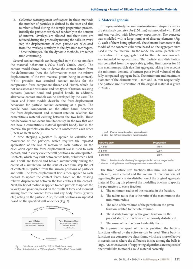
A time stepping algorithm is applied to calculate the movement of the particles, which requires the repeated application of the law of motion to each particle. In the calculation cycle the force-displacement law is used to each contact, and in every cycle the wall positions are also updated. Contacts, which may exist between two balls, or between a ball and a wall, are formed and broken automatically during the course of a simulation. At the start of each time step the set of contacts is updated from the known positions of particles and walls. The force-displacement law is then applied to each contact to update the contact forces based on the existing relative displacement between the two entities at the contact. Next, the law of motion is applied to each particle to update the velocity and position, based on the resultant force and moment arising from the contact forces and any body forces (gravity etc.) acting on the particle. Also, the wall positions are updated based on the specified wall velocities (Fig. 1).

Fig. 1. Calculation cycle in PFC3D (PFC3D User’s Guide, 2008) 1. ábra Számítási ciklus a PFC3D szoftverben (PFC3D User’s Guide, 2008)

3. Material genesisIn the present study the compression stress-strain performance

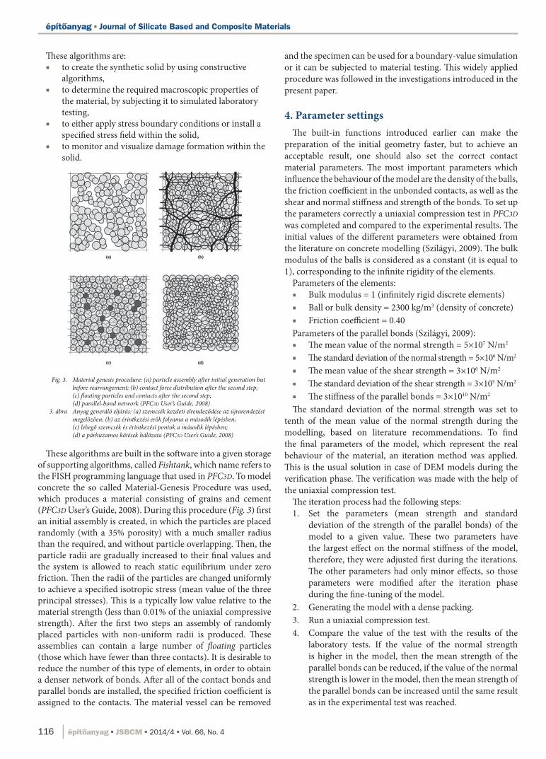
of a standard concrete cube (150 mm) was modelled with DEM and was verified with laboratory experiments. The concrete was modelled with a large number of discrete elements (Fig. 2), each of them being spherical. The element diameters in the model of the concrete cube were based on the aggregate sizes used in the real material. In the model the actual particle size distribution of the aggregate used for the reference concrete was intended to approximate. The particle size distribution was compiled from the applicable grading limit curves for 16 mm maximum particle size flint aggregate, taking into account the minimum demand of cement paste (void volume) of the fully compacted aggregate bulk. The minimum and maximum diameter of the elements was 1 mm and 16 mm respectively. The particle size distribution of the original material is given in Table 1.

Fig. 2. Discrete element model of a concrete cube 2. ábra Egy beton kocka diszkrét elemes modellje

Particle size Proportion0-4 mm 40 %4-8 mm 22 %8-16 mm 38 %

Table 1. Particle size distribution of the aggregate in the concrete sample studied 1. táblázat A vizsgált beton adalékanyagának szemcseméret eloszlása

The three particle size fractions (0-4 mm, 4-8 mm and 8-16 mm) were created and the volume of fractions was set regarding the particle size distribution of the original aggregate material. During this phase of the modelling one has to specify five parameters to every fraction:

1. The minimum radius of the material in the fraction.2. The radius ratio; that is the ratio of the maximum to the

minimum radius.3. The ratio of the volume of the particles in the given

fraction, related to the total volume. 4. The distribution type of the given fraction. In the

present study the fractions are uniformly distributed.5. The name of the fractions to identify them. To improve the speed of the computation, the built-in

functions offered by the software can be used. These built-in functions use constructive algorithms, which are more effective in certain cases where the difference in size among the balls is large. An extensive set of supporting algorithms are required if one would like to model a solid material correctly.

ÉPA 2014_4.indd 115 2015.01.19. 15:34:56



These algorithms are:■■ to create the synthetic solid by using constructive

algorithms,■■ to determine the required macroscopic properties of

the material, by subjecting it to simulated laboratory testing,

■■ to either apply stress boundary conditions or install a specified stress field within the solid,

■■ to monitor and visualize damage formation within the solid.

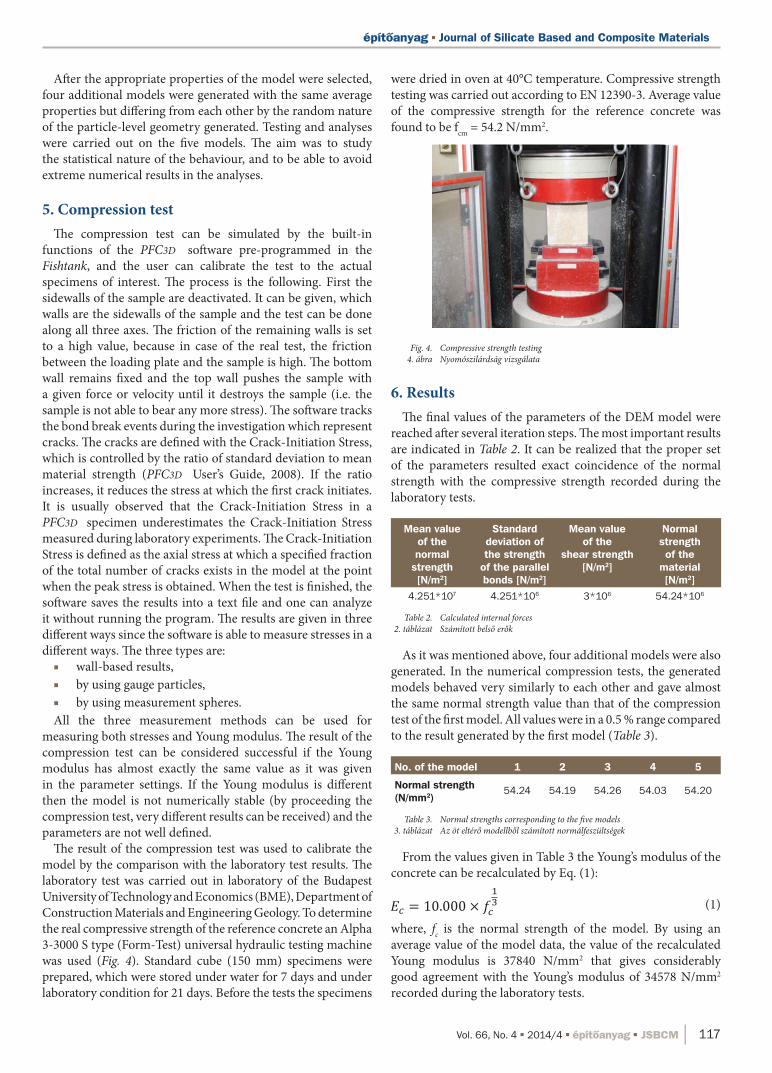
Fig. 3. Material genesis procedure: (a) particle assembly after initial generation but before rearrangement; (b) contact force distribution after the second step; (c) floating particles and contacts after the second step; (d) parallel-bond network (PFC3D User’s Guide, 2008)

3. ábra Anyag generáló eljárás: (a) szemcsék kezdeti elrendeződése az újrarendezést megelőzően; (b) az érintkezési erők folyama a második lépésben; (c) lebegő szemcsék és érintkezési pontok a második lépésben; (d) a párhuzamos kötések hálózata (PFC3D User’s Guide, 2008)

These algorithms are built in the software into a given storage of supporting algorithms, called Fishtank, which name refers to the FISH programming language that used in PFC3D. To model concrete the so called Material-Genesis Procedure was used, which produces a material consisting of grains and cement (PFC3D User’s Guide, 2008). During this procedure (Fig. 3) first an initial assembly is created, in which the particles are placed randomly (with a 35% porosity) with a much smaller radius than the required, and without particle overlapping. Then, the particle radii are gradually increased to their final values and the system is allowed to reach static equilibrium under zero friction. Then the radii of the particles are changed uniformly to achieve a specified isotropic stress (mean value of the three principal stresses). This is a typically low value relative to the material strength (less than 0.01% of the uniaxial compressive strength). After the first two steps an assembly of randomly placed particles with non-uniform radii is produced. These assemblies can contain a large number of floating particles (those which have fewer than three contacts). It is desirable to reduce the number of this type of elements, in order to obtain a denser network of bonds. After all of the contact bonds and parallel bonds are installed, the specified friction coefficient is assigned to the contacts. The material vessel can be removed

and the specimen can be used for a boundary-value simulation or it can be subjected to material testing. This widely applied procedure was followed in the investigations introduced in the present paper.

4. Parameter settingsThe built-in functions introduced earlier can make the

preparation of the initial geometry faster, but to achieve an acceptable result, one should also set the correct contact material parameters. The most important parameters which influence the behaviour of the model are the density of the balls, the friction coefficient in the unbonded contacts, as well as the shear and normal stiffness and strength of the bonds. To set up the parameters correctly a uniaxial compression test in PFC3D was completed and compared to the experimental results. The initial values of the different parameters were obtained from the literature on concrete modelling (Szilágyi, 2009). The bulk modulus of the balls is considered as a constant (it is equal to 1), corresponding to the infinite rigidity of the elements.

Parameters of the elements: ■■ Bulk modulus = 1 (infinitely rigid discrete elements)■■ Ball or bulk density = 2300 kg/m3 (density of concrete) ■■ Friction coefficient = 0.40

Parameters of the parallel bonds (Szilágyi, 2009):■■ The mean value of the normal strength = 5×107 N/m2 ■■ The standard deviation of the normal strength = 5×106 N/m2

■■ The mean value of the shear strength = 3×106 N/m2 ■■ The standard deviation of the shear strength = 3×105 N/m2

■■ The stiffness of the parallel bonds = 3×1010 N/m2

The standard deviation of the normal strength was set to tenth of the mean value of the normal strength during the modelling, based on literature recommendations. To find the final parameters of the model, which represent the real behaviour of the material, an iteration method was applied. This is the usual solution in case of DEM models during the verification phase. The verification was made with the help of the uniaxial compression test.

The iteration process had the following steps:1. Set the parameters (mean strength and standard

deviation of the strength of the parallel bonds) of the model to a given value. These two parameters have the largest effect on the normal stiffness of the model, therefore, they were adjusted first during the iterations. The other parameters had only minor effects, so those parameters were modified after the iteration phase during the fine-tuning of the model.

2. Generating the model with a dense packing.3. Run a uniaxial compression test.4. Compare the value of the test with the results of the

laboratory tests. If the value of the normal strength is higher in the model, then the mean strength of the parallel bonds can be reduced, if the value of the normal strength is lower in the model, then the mean strength of the parallel bonds can be increased until the same result as in the experimental test was reached.

ÉPA 2014_4.indd 116 2015.01.19. 15:34:56



After the appropriate properties of the model were selected, four additional models were generated with the same average properties but differing from each other by the random nature of the particle-level geometry generated. Testing and analyses were carried out on the five models. The aim was to study the statistical nature of the behaviour, and to be able to avoid extreme numerical results in the analyses.

5. Compression testThe compression test can be simulated by the built-in

functions of the PFC3D software pre-programmed in the Fishtank, and the user can calibrate the test to the actual specimens of interest. The process is the following. First the sidewalls of the sample are deactivated. It can be given, which walls are the sidewalls of the sample and the test can be done along all three axes. The friction of the remaining walls is set to a high value, because in case of the real test, the friction between the loading plate and the sample is high. The bottom wall remains fixed and the top wall pushes the sample with a given force or velocity until it destroys the sample (i.e. the sample is not able to bear any more stress). The software tracks the bond break events during the investigation which represent cracks. The cracks are defined with the Crack-Initiation Stress, which is controlled by the ratio of standard deviation to mean material strength (PFC3D User’s Guide, 2008). If the ratio increases, it reduces the stress at which the first crack initiates. It is usually observed that the Crack-Initiation Stress in a PFC3D specimen underestimates the Crack-Initiation Stress measured during laboratory experiments. The Crack-Initiation Stress is defined as the axial stress at which a specified fraction of the total number of cracks exists in the model at the point when the peak stress is obtained. When the test is finished, the software saves the results into a text file and one can analyze it without running the program. The results are given in three different ways since the software is able to measure stresses in a different ways. The three types are:■■ wall-based results,■■ by using gauge particles,■■ by using measurement spheres.

All the three measurement methods can be used for measuring both stresses and Young modulus. The result of the compression test can be considered successful if the Young modulus has almost exactly the same value as it was given in the parameter settings. If the Young modulus is different then the model is not numerically stable (by proceeding the compression test, very different results can be received) and the parameters are not well defined.

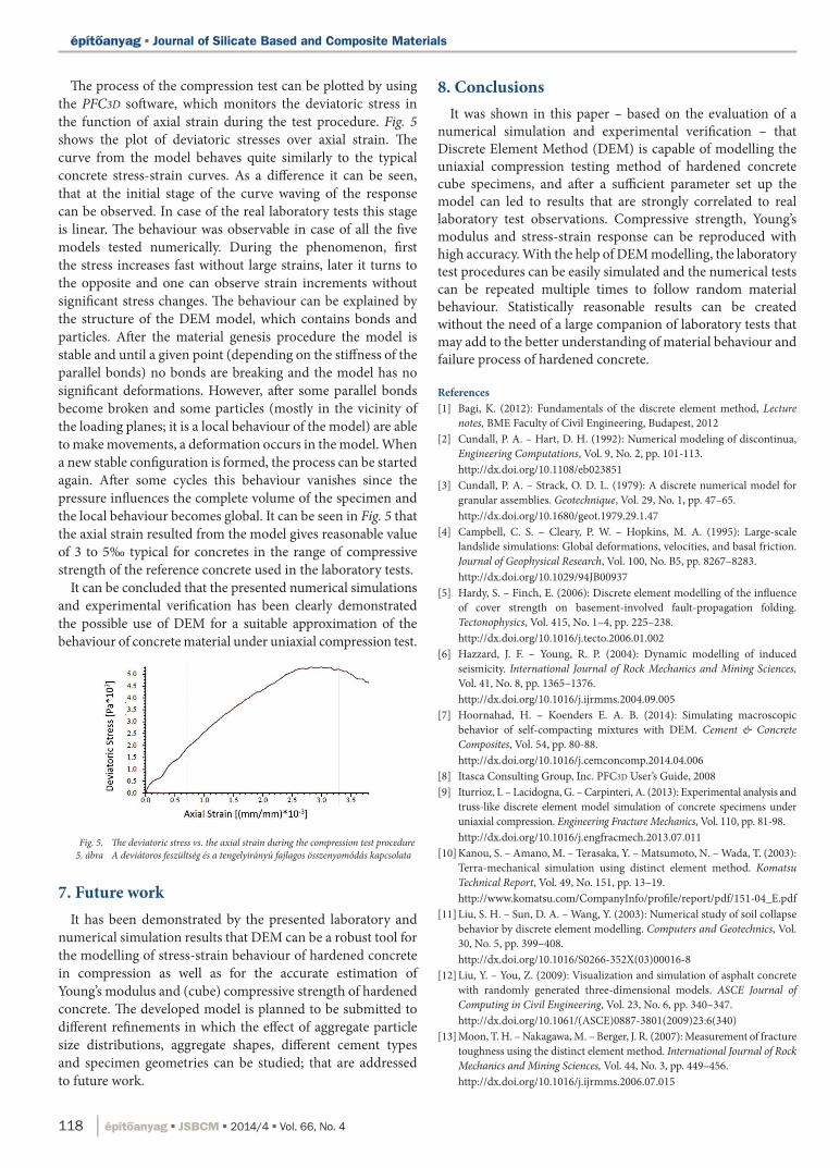
The result of the compression test was used to calibrate the model by the comparison with the laboratory test results. The laboratory test was carried out in laboratory of the Budapest University of Technology and Economics (BME), Department of Construction Materials and Engineering Geology. To determine the real compressive strength of the reference concrete an Alpha 3-3000 S type (Form-Test) universal hydraulic testing machine was used (Fig. 4). Standard cube (150 mm) specimens were prepared, which were stored under water for 7 days and under laboratory condition for 21 days. Before the tests the specimens

were dried in oven at 40°C temperature. Compressive strength testing was carried out according to EN 12390-3. Average value of the compressive strength for the reference concrete was found to be fcm = 54.2 N/mm2.

Fig. 4. Compressive strength testing 4. ábra Nyomószilárdság vizsgálata

6. ResultsThe final values of the parameters of the DEM model were

reached after several iteration steps. The most important results are indicated in Table 2. It can be realized that the proper set of the parameters resulted exact coincidence of the normal strength with the compressive strength recorded during the laboratory tests.

Mean value of the normal

strength [N/m2]

Standard deviation of the strength

of the parallel bonds [N/m2]

Mean value of the

shear strength [N/m2]

Normal strength of the

material [N/m2]

4.251*107 4.251*106 3*106 54.24*106

Table 2. Calculated internal forces 2. táblázat Számított belső erők

As it was mentioned above, four additional models were also generated. In the numerical compression tests, the generated models behaved very similarly to each other and gave almost the same normal strength value than that of the compression test of the first model. All values were in a 0.5 % range compared to the result generated by the first model (Table 3).

No. of the model 1 2 3 4 5

Normal strength (N/mm2)

54.24 54.19 54.26 54.03 54.20

Table 3. Normal strengths corresponding to the five models 3. táblázat Az öt eltérő modellből számított normálfeszültségek

From the values given in Table 3 the Young’s modulus of the concrete can be recalculated by Eq. (1):

(1)

where, fc is the normal strength of the model. By using an average value of the model data, the value of the recalculated Young modulus is 37840 N/mm2 that gives considerably good agreement with the Young’s modulus of 34578 N/mm2 recorded during the laboratory tests.

ÉPA 2014_4.indd 117 2015.01.19. 15:34:56



The process of the compression test can be plotted by using the PFC3D software, which monitors the deviatoric stress in the function of axial strain during the test procedure. Fig. 5 shows the plot of deviatoric stresses over axial strain. The curve from the model behaves quite similarly to the typical concrete stress-strain curves. As a difference it can be seen, that at the initial stage of the curve waving of the response can be observed. In case of the real laboratory tests this stage is linear. The behaviour was observable in case of all the five models tested numerically. During the phenomenon, first the stress increases fast without large strains, later it turns to the opposite and one can observe strain increments without significant stress changes. The behaviour can be explained by the structure of the DEM model, which contains bonds and particles. After the material genesis procedure the model is stable and until a given point (depending on the stiffness of the parallel bonds) no bonds are breaking and the model has no significant deformations. However, after some parallel bonds become broken and some particles (mostly in the vicinity of the loading planes; it is a local behaviour of the model) are able to make movements, a deformation occurs in the model. When a new stable configuration is formed, the process can be started again. After some cycles this behaviour vanishes since the pressure influences the complete volume of the specimen and the local behaviour becomes global. It can be seen in Fig. 5 that the axial strain resulted from the model gives reasonable value of 3 to 5‰ typical for concretes in the range of compressive strength of the reference concrete used in the laboratory tests.

It can be concluded that the presented numerical simulations and experimental verification has been clearly demonstrated the possible use of DEM for a suitable approximation of the behaviour of concrete material under uniaxial compression test.

Fig. 5. The deviatoric stress vs. the axial strain during the compression test procedure 5. ábra A deviátoros feszültség és a tengelyirányú fajlagos összenyomódás kapcsolata

7. Future workIt has been demonstrated by the presented laboratory and

numerical simulation results that DEM can be a robust tool for the modelling of stress-strain behaviour of hardened concrete in compression as well as for the accurate estimation of Young’s modulus and (cube) compressive strength of hardened concrete. The developed model is planned to be submitted to different refinements in which the effect of aggregate particle size distributions, aggregate shapes, different cement types and specimen geometries can be studied; that are addressed to future work.

8. ConclusionsIt was shown in this paper – based on the evaluation of a

numerical simulation and experimental verification – that Discrete Element Method (DEM) is capable of modelling the uniaxial compression testing method of hardened concrete cube specimens, and after a sufficient parameter set up the model can led to results that are strongly correlated to real laboratory test observations. Compressive strength, Young’s modulus and stress-strain response can be reproduced with high accuracy. With the help of DEM modelling, the laboratory test procedures can be easily simulated and the numerical tests can be repeated multiple times to follow random material behaviour. Statistically reasonable results can be created without the need of a large companion of laboratory tests that may add to the better understanding of material behaviour and failure process of hardened concrete.

References[1] Bagi, K. (2012): Fundamentals of the discrete element method, Lecture

notes, BME Faculty of Civil Engineering, Budapest, 2012[2] Cundall, P. A. – Hart, D. H. (1992): Numerical modeling of discontinua,

Engineering Computations, Vol. 9, No. 2, pp. 101-113. http://dx.doi.org/10.1108/eb023851 [3] Cundall, P. A. – Strack, O. D. L. (1979): A discrete numerical model for

granular assemblies. Geotechnique, Vol. 29, No. 1, pp. 47–65. http://dx.doi.org/10.1680/geot.1979.29.1.47 [4] Campbell, C. S. – Cleary, P. W. – Hopkins, M. A. (1995): Large-scale

landslide simulations: Global deformations, velocities, and basal friction. Journal of Geophysical Research, Vol. 100, No. B5, pp. 8267–8283.

http://dx.doi.org/10.1029/94JB00937 [5] Hardy, S. – Finch, E. (2006): Discrete element modelling of the influence

of cover strength on basement-involved fault-propagation folding. Tectonophysics, Vol. 415, No. 1–4, pp. 225–238.

http://dx.doi.org/10.1016/j.tecto.2006.01.002 [6] Hazzard, J. F. – Young, R. P. (2004): Dynamic modelling of induced

seismicity. International Journal of Rock Mechanics and Mining Sciences, Vol. 41, No. 8, pp. 1365–1376.

http://dx.doi.org/10.1016/j.ijrmms.2004.09.005 [7] Hoornahad, H. – Koenders E. A. B. (2014): Simulating macroscopic

behavior of self-compacting mixtures with DEM. Cement & Concrete Composites, Vol. 54, pp. 80-88.

http://dx.doi.org/10.1016/j.cemconcomp.2014.04.006 [8] Itasca Consulting Group, Inc. PFC3D User’s Guide, 2008[9] Iturrioz, I. – Lacidogna, G. – Carpinteri, A. (2013): Experimental analysis and

truss-like discrete element model simulation of concrete specimens under uniaxial compression. Engineering Fracture Mechanics, Vol. 110, pp. 81-98.

http://dx.doi.org/10.1016/j.engfracmech.2013.07.011 [10] Kanou, S. – Amano, M. – Terasaka, Y. – Matsumoto, N. – Wada, T. (2003):

Terra-mechanical simulation using distinct element method. Komatsu Technical Report, Vol. 49, No. 151, pp. 13–19.

http://www.komatsu.com/CompanyInfo/profile/report/pdf/151-04_E.pdf [11] Liu, S. H. – Sun, D. A. – Wang, Y. (2003): Numerical study of soil collapse

behavior by discrete element modelling. Computers and Geotechnics, Vol. 30, No. 5, pp. 399–408.

http://dx.doi.org/10.1016/S0266-352X(03)00016-8 [12] Liu, Y. – You, Z. (2009): Visualization and simulation of asphalt concrete

with randomly generated three-dimensional models. ASCE Journal of Computing in Civil Engineering, Vol. 23, No. 6, pp. 340–347.

http://dx.doi.org/10.1061/(ASCE)0887-3801(2009)23:6(340) [13] Moon, T. H. – Nakagawa, M. – Berger, J. R. (2007): Measurement of fracture

toughness using the distinct element method. International Journal of Rock Mechanics and Mining Sciences, Vol. 44, No. 3, pp. 449–456.

http://dx.doi.org/10.1016/j.ijrmms.2006.07.015

ÉPA 2014_4.indd 118 2015.01.19. 15:34:57

http://dx.doi.org/10.1016/S0266-352X(03)00016-8

http://dx.doi.org/10.1061/(ASCE)0887-3801(2009)23:6(340)



[14] Potyondy, D. O. – Cundall, P. A. (2004): A bonded-particle model for rock. International Journal of Rock Mechanics and Mining Sciences, Vol. 41, No. 8, pp. 1329–1364.

http://dx.doi.org/10.1016/j.ijrmms.2004.09.011 [15] Remond, S. – Pizette, P. (2014): A DEM hard-core soft-shell model for the

simulation of concrete flow. Cement and Concrete Research, Vol. 58, pp. 169-178. http://dx.doi.org/10.1016/j.cemconres.2014.01.022 [16] Riera, J. D. – Miguel, L. F. F. – Iturrioz, I. (2014): Assessment of Brazilian

tensile test by means of the truss-like Discrete Element Method (DEM) with imperfect mesh. Engineering Structures, Vol. 81, pp. 10-21.

http://dx.doi.org/10.1016/j.engstruct.2014.09.036 [17] Shyshko, S. – Mechtcherine, V. (2013): Developing a Discrete Element

Model for simulating fresh concrete: Experimental investigation and modelling of interactions between discrete aggregate particles with fine mortar between them. Construction and Building Materials, Vol. 47, pp. 601-615. http://dx.doi.org/10.1016/j.conbuildmat.2013.05.071

[18] Szilágyi, K. (2009): DEM modelling of the Brinell-testing of concrete, Micromechanics of granular media – Manuscript, BME Faculty of Civil Engineering, Budapest, 2009

[19] Tran, V. T. – Donzé, F.-V. – Marin, P. (2011): A discrete element model of concrete under high triaxial loading. Cement & Concrete Composites, Vol. 33, No. 9, pp. 936–948.

http://dx.doi.org/10.1016/j.cemconcomp.2011.01.003 [20] Yao, M. – Anandarajah, A. (2003): Three-dimensional discrete element

method of analysis of clays. Journal of Engineering Mechanics, Vol. 129, No. 6, pp. 585–596.

http://dx.doi.org/10.1061/(ASCE)0733-9399(2003)129:6(585) [21] You, Z. – Adhikari, S. – Dai, Q. (2008): Three-dimensional discrete

element models for asphalt mixtures. Journal of Engineering Mechanics, Vol. 134, No. 12, pp. 1053–1063.

http://dx.doi.org/10.1061/(ASCE)0733-9399(2008)134:12(1053) [22] You, Z. – Buttlar, W. G. (2004): Discrete element modeling to predict the

modulus of asphalt concrete mixtures. ASCE Journal of Materials in Civil Engineering, Vol. 16, No. 2, pp. 140–146.


[23] Zhu, H. P. – Zhou, Z. Y. – Yang, R. Y. – Yu, A. B. (2007): Discrete particle simulation of particulate systems: Theoretical developments. Chemical Engineering Science, Vol. 62, No. 13, pp. 3378–3396.

http://dx.doi.org/10.1016/j.ces.2006.12.089 [24] Zivaljic, N. – Nikolic, Z. – Smoljanovic, H. (2014): Computational aspects

of the combined finite–discrete element method in modelling of plane reinforced concrete structures. Engineering Fracture Mechanics, Vol. 131, pp. 669-686.

http://dx.doi.org/10.1016/j.engfracmech.2014.10.017

Ref.:Gyurkó, Zoltán – Bagi, Katalin – Borosnyói, Adorján: Discrete

Element Modelling of uniaxial compression test of hardened concrete Építő anyag – Journal of Silicate Based and Composite Materials,

Vol. 66, No. 4 (2014), 113–119. p. http://dx.doi.org/10.14382/epitoanyag-jsbcm.2014.21

Megszilárdult beton nyomószilárdság vizsgálatának modellezése diszkrét elemes módszerrelA cikk megszilárdult beton nyomószilárdságának numeri-kus modellezését ismerteti a diszkrét elemes módszer (Dem) felhasználásával. A diszkrét elemes módszer rövid bemutatását követően a numerikus modell felépítését és a nyomószilárdság vizsgálat numerikus szimulációjának eredményeit ismertetjük. A numerikus kísérlet eredményeit tényleges nyomószilárdság vizsgálat eredményeivel hason-lítjuk össze. Bemutatjuk, hogy a diszkrét elemes módszer-rel konstruálható olyan szemcseösszetétel, amely pontosan követi a vizsgált beton adalékanyagának szemeloszlását, numerikusan stabil, és paraméterei beállíthatók oly módon, hogy a tényleges nyomószilárdság és rugalmassági modulus csaknem teljes pontossággal előállíthatóvá válik.kulcsszavak: diszkrét elemes módszer, beton, feszültség-alakváltozás, nyomószilárdság

Dramatically Improved Performance• Fastest time-to-solution available today, with the latest in parallel algorithms.• Automatically tuned spatial searching and contact detection for complex particle-size distributions

and rapid granular flow problems.

Simplified Model Creation• Rhino CAD front end for complex wall and particle shape design. Rhino is the most user-friendly

solid modeling package in the market. • Practical and straightforward material property assignments with the Contact Model Assignment

Table (CMAT) concept.• Simple commands for controlling particle sample size distribution, target porosity, etc.• Powerful periodic space support for particles and contact models.• Discrete Fracture Networks (DFNs) can be generated using imported fracture statistics.

Improved Graphical User Interface• Query tools for interactive display of particle properties (e.g., ID, radius, velocity, spin, etc.).• Advanced post-processing including easy-to-use and customize high-quality animation scripts.• Built-in text editor for writing data files and scripts, including syntax highlighting and validation.• Stereonet and rosette charts for rock mechanics applications.

More Powerful Scripting• Deep scripting with both Python and FISH gives access to every variable and sub-model in the

simulation. • Extended FISH language and libraries including arguments, local variables, new data types,

simplified looping constructs and FISH in command lines.• A FISH-variable explorer allows users to view variable values during model creation and simulation.

New Physics • Long-range interactions based on distance at which contacts are created (Electro-magnetic, gravity

and capillary interactions).• Easy coupling with any open-source Computational Fluid Dynamics software or computational force

field simulator.• Easy gradual addition of any quantifiable physics using deep scripting.• Best-documented, most trusted and most quoted DEM software over the last 15 years• Available both in 2D and 3D.

Itasca’s new DEM Product is designed for parallel performance, ease-of-use and versatility.

www.itascacg.com

© 2014 Itasca Consulting Group, Inc., an Itasca International company ICG

14

-CRD

-PFC

50

0-0

2














www.itascacg.com


14-C

RD-P

FC500-0

2

Dramatically Improved Performance• Fastesttime-to-solutionavailabletoday,withthelatestinparallelalgorithms.• Automatically tuned spatial searching and contact detection for complex particle-sizedistributionsandrapidgranularflowproblems.

Simplified Model Creation• Rhino CAD front end for complex wall and particle shape design. Rhino is the most user-friendlysolidmodelingpackageinthemarket.

• Practical and straightforward material property assignments with the Contact ModelAssignmentTable(CMAT)concept.

• Simplecommandsforcontrollingparticlesamplesizedistribution,targetporosity,etc.• Powerfulperiodicspacesupportforparticlesandcontactmodels.• DiscreteFractureNetworks(DFNs)canbegeneratedusingimportedfracturestatistics.

Improved Graphical User Interface• Querytoolsforinteractivedisplayofparticleproperties(e.g.,ID,radius,velocity,spin,etc.).• Advancedpost-processingincludingeasy-to-useandcustomizehigh-qualityanimationscripts.• Built-intexteditorforwritingdatafilesandscripts,includingsyntaxhighlightingandvalidation.• Stereonetandrosettechartsforrockmechanicsapplications.

More Powerful Scripting• Deep scripting with both Python and FISH gives access to every variable and sub-model inthesimulation.

• Extended FISH language and libraries including arguments, local variables, new datatypes,simplifiedloopingconstructsandFISHincommandlines.

• AFISH-variableexplorerallowsuserstoviewvariablevaluesduringmodelcreationandsimulation.

New Physics• Long-range interactions based on distance at which contacts are created (Electro-magnetic,gravityandcapillaryinteractions).

• Easy couplingwith any open-source Computational Fluid Dynamics software or computationalforcefieldsimulator.

• Easygradualadditionofanyquantifiablephysicsusingdeepscripting.• Best-documented,mosttrustedandmostquotedDEMsoftwareoverthelast15years.• Availablebothin2Dand3D.














www.itascacg.com


14-C

RD-P

FC500-0

2


ÉPA 2014_4.indd 119 2015.01.19. 15:34:57




Documents

Discrete element modelling Zoltán Gyurkó of uniaxial