Introduction to Deep Learning

ENEE698A : Machine Learning Seminar

Raviteja Vemulapalli

Image credit: [LeCun 1998]

Resources

Unsupervised feature learning and deep learning (UFLDL) tutorial(http://ufldl.Stanford.edu/wiki/index.php/UFLDL_Tutorial)

Y. Bengio, “Learning Deep Architectures for AI“, Foundations and Trends in Machine Learning, Vol. 2, No. 1, pp. 1–127, 2009, Now publishers.

Overview Linear, Logistic and Softmax regression

Feed forward neural networks

Why deep models?

Why is training deep networks (except CNNs) difficult?

What makes convolutional neural networks (CNNs) relatively easier to train?

How are deep networks trained today?

Autoencoders and Denoising Autoencoders

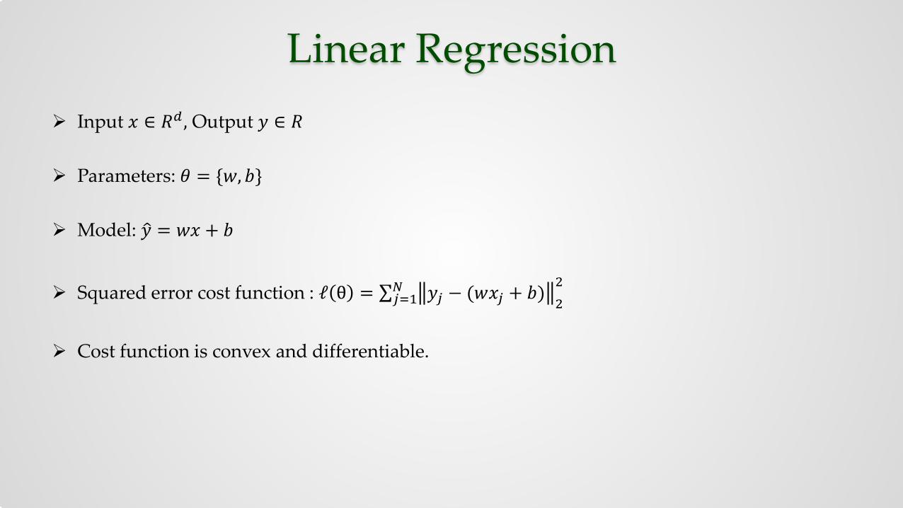
Linear Regression Input 𝑥𝑥 ∈ 𝑅𝑅𝑑𝑑 , Output 𝑦𝑦 ∈ 𝑅𝑅

Parameters: 𝜃𝜃 = {𝑤𝑤, 𝑏𝑏}

Model: �𝑦𝑦 = 𝑤𝑤𝑥𝑥 + 𝑏𝑏

Squared error cost function : ℓ θ = ∑𝑗𝑗=1𝑁𝑁 𝑦𝑦𝑗𝑗 − (𝑤𝑤𝑥𝑥𝑗𝑗 + 𝑏𝑏)22

Cost function is convex and differentiable.

Logistic Regression Used for binary classification.

Input 𝑥𝑥 ∈ 𝑅𝑅𝑑𝑑 , Output 𝑦𝑦 ∈ {0,1}

Parameters: 𝜃𝜃 = {𝑤𝑤, 𝑏𝑏}

Model: 𝑃𝑃 𝑦𝑦 = 1 𝑥𝑥,𝜃𝜃 = 11+𝑒𝑒−(𝑤𝑤𝑥𝑥+𝑏𝑏)

NLL cost function: ℓ θ = −log ∏𝑗𝑗=1𝑁𝑁 𝑃𝑃 𝑦𝑦 = 𝑦𝑦𝑗𝑗| 𝑥𝑥𝑗𝑗 ,𝜃𝜃 = −∑𝑗𝑗=1𝑁𝑁 log 𝑃𝑃 𝑦𝑦 = 𝑦𝑦𝑗𝑗| 𝑥𝑥𝑗𝑗 ,𝜃𝜃

Cost function is convex and differentiable.

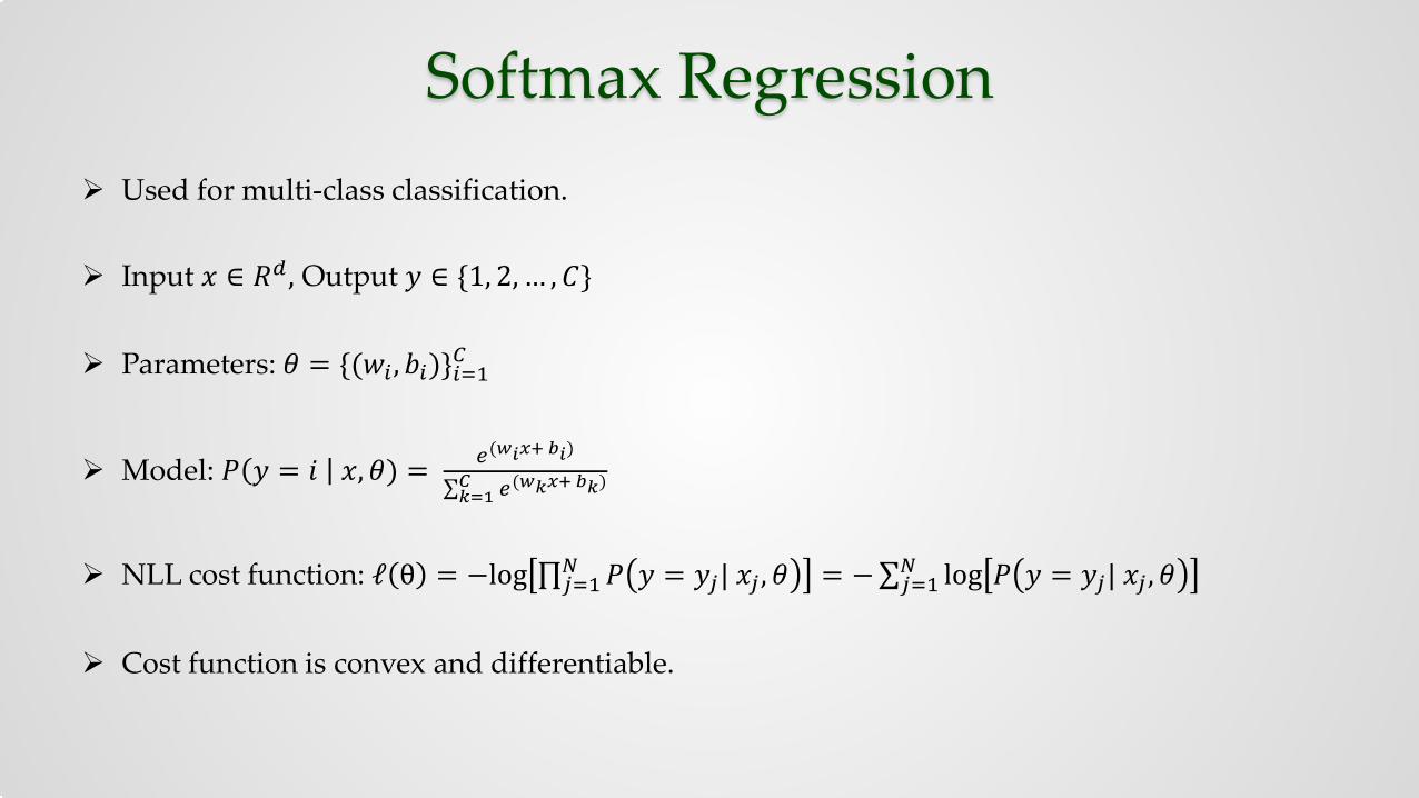
Softmax Regression Used for multi-class classification.

Input 𝑥𝑥 ∈ 𝑅𝑅𝑑𝑑 , Output 𝑦𝑦 ∈ {1, 2, … ,𝐶𝐶}

Parameters: 𝜃𝜃 = {(𝑤𝑤𝑖𝑖 ,𝑏𝑏𝑖𝑖)}𝑖𝑖=1𝐶𝐶

Model: 𝑃𝑃 𝑦𝑦 = 𝑖𝑖 𝑥𝑥,𝜃𝜃) = 𝑒𝑒(𝑤𝑤𝑖𝑖𝑥𝑥+ 𝑏𝑏𝑖𝑖)

∑𝑘𝑘=1𝐶𝐶 𝑒𝑒(𝑤𝑤𝑘𝑘𝑥𝑥+ 𝑏𝑏𝑘𝑘)

NLL cost function: ℓ θ = −log ∏𝑗𝑗=1𝑁𝑁 𝑃𝑃 𝑦𝑦 = 𝑦𝑦𝑗𝑗| 𝑥𝑥𝑗𝑗 ,𝜃𝜃 = −∑𝑗𝑗=1𝑁𝑁 log 𝑃𝑃 𝑦𝑦 = 𝑦𝑦𝑗𝑗| 𝑥𝑥𝑗𝑗 ,𝜃𝜃

Cost function is convex and differentiable.

Regularization & Optimization

ℓ2-Regularization (Weight decay)

min𝑤𝑤,𝑏𝑏

[ℓ 𝑤𝑤, 𝑏𝑏 + 𝜆𝜆 𝑤𝑤 22]

Regularization helps to avoid overfitting.

ℓ2-Regularization is equivalent to MAP estimation with zero-mean Gaussian prior on 𝑤𝑤.

Optimization [ℓ 𝑤𝑤, 𝑏𝑏 + 𝜆𝜆 𝑤𝑤 2

2] is convex and differentiable in the case of linear, logistic and softmaxregression.

Gradient based optimization techniques can be used to find the global optimum.

Feed Forward Neural Networks

Feed Forward Neural NetworksArtificial neuron

𝑔𝑔 is a non-linear function referred to as activation function.

Logistic and hyperbolic tangent functions are two commonly used activation functions.

Hyperbolic tangent functionLogistic function

Image credit: UFLDL Tutorial

ℎ𝑤𝑤,𝑏𝑏(𝑥𝑥) = 𝑔𝑔(𝑤𝑤𝑥𝑥 + 𝑏𝑏)

Feed Forward Neural NetworksNeural network with 2 hidden layers

Note that if the activation function is linear, then the entire neural network is effectively equivalent to the output layer.

Image credit: UFLDL Tutorial

Input layer(3 inputs)

Output layer(2 units)

Hidden layer 1(3 units)

Hidden layer 2(2 units)

Output layer

Application ModelRegression Linear regression

Binary classification Logistic regression

Multi-class classification Softmax regression

Non-linear (logistic or tanh)

Feed Forward Neural Networks - Prediction Forward propagation

L – Number of layers (including input and output layers) 𝑛𝑛𝑖𝑖 - Number of units in 𝑖𝑖𝑡𝑡𝑡 layer 𝑎𝑎(𝑖𝑖) ∈ 𝑅𝑅𝑛𝑛𝑖𝑖 - Output of 𝑖𝑖𝑡𝑡𝑡 layer 𝑊𝑊(𝑖𝑖) ∈ 𝑅𝑅𝑛𝑛𝑖𝑖+1×𝑛𝑛𝑖𝑖 ,𝑏𝑏(𝑖𝑖) ∈ 𝑅𝑅𝑛𝑛𝑖𝑖+1 - Parameters of the mapping function from layer 𝑖𝑖 to 𝑖𝑖 + 1. 𝑆𝑆 - Output layer model (linear, logistic or softmax)

𝑎𝑎(1) = 𝑥𝑥

𝑎𝑎(2) = 𝑔𝑔(𝑊𝑊 1 𝑎𝑎 1 + 𝑏𝑏 1 )

𝑎𝑎(𝐿𝐿−1) = 𝑔𝑔(𝑊𝑊 𝐿𝐿−2 𝑎𝑎 𝐿𝐿−2 + 𝑏𝑏 𝐿𝐿−2 )...

ℎ𝑊𝑊,𝑏𝑏 𝑥𝑥 = 𝑎𝑎(𝐿𝐿) = 𝑆𝑆(𝑊𝑊 𝐿𝐿−1 𝑎𝑎 𝐿𝐿−1 + 𝑏𝑏 𝐿𝐿−1 )

𝑎𝑎(1) 𝑎𝑎(2) 𝑎𝑎(3) 𝑎𝑎(4)

Image credit: UFLDL Tutorial

𝑊𝑊(1), 𝑏𝑏(1)

𝑊𝑊(2), 𝑏𝑏(2)

𝑊𝑊(3), 𝑏𝑏(3)

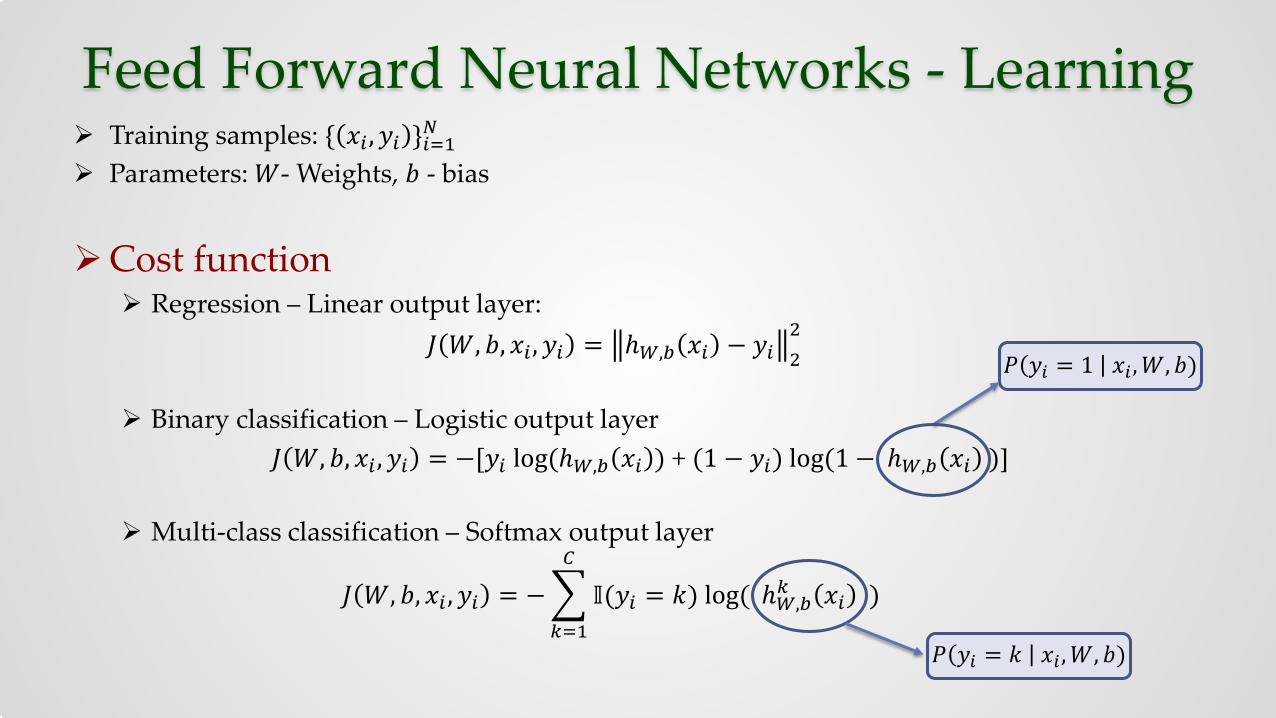
Feed Forward Neural Networks - Learning Training samples: { 𝑥𝑥𝑖𝑖 ,𝑦𝑦𝑖𝑖 }𝑖𝑖=1𝑁𝑁

Parameters: 𝑊𝑊- Weights, 𝑏𝑏 - bias

Cost function Regression – Linear output layer:

𝐽𝐽 𝑊𝑊, 𝑏𝑏, 𝑥𝑥𝑖𝑖 ,𝑦𝑦𝑖𝑖 = ℎ𝑊𝑊,𝑏𝑏 𝑥𝑥𝑖𝑖 − 𝑦𝑦𝑖𝑖 22

Binary classification – Logistic output layer𝐽𝐽 𝑊𝑊, 𝑏𝑏, 𝑥𝑥𝑖𝑖 ,𝑦𝑦𝑖𝑖 = −[𝑦𝑦𝑖𝑖 log(ℎ𝑊𝑊,𝑏𝑏 𝑥𝑥𝑖𝑖 ) + (1 − 𝑦𝑦𝑖𝑖) log(1 − ℎ𝑊𝑊,𝑏𝑏 𝑥𝑥𝑖𝑖 )]

Multi-class classification – Softmax output layer

𝐽𝐽 𝑊𝑊, 𝑏𝑏, 𝑥𝑥𝑖𝑖 ,𝑦𝑦𝑖𝑖 = −�𝑘𝑘=1

𝐶𝐶

𝕀𝕀(𝑦𝑦𝑖𝑖 = 𝑘𝑘) log( ℎ𝑊𝑊,𝑏𝑏𝑘𝑘 𝑥𝑥𝑖𝑖 )

𝑃𝑃 𝑦𝑦𝑖𝑖 = 1 𝑥𝑥𝑖𝑖 ,𝑊𝑊, 𝑏𝑏)

𝑃𝑃 𝑦𝑦𝑖𝑖 = 𝑘𝑘 𝑥𝑥𝑖𝑖 ,𝑊𝑊, 𝑏𝑏)

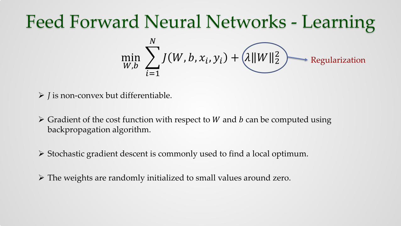
Feed Forward Neural Networks - Learning

min𝑊𝑊,𝑏𝑏

�𝑖𝑖=1

𝑁𝑁

𝐽𝐽 𝑊𝑊, 𝑏𝑏, 𝑥𝑥𝑖𝑖 ,𝑦𝑦𝑖𝑖 + 𝜆𝜆 𝑊𝑊 22

J is non-convex but differentiable.

Gradient of the cost function with respect to 𝑊𝑊 and 𝑏𝑏 can be computed using backpropagation algorithm.

Stochastic gradient descent is commonly used to find a local optimum.

The weights are randomly initialized to small values around zero.

Regularization

How powerful are neural networks?

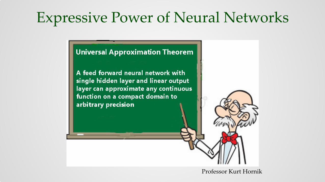
Expressive Power of Neural Networks

Professor Kurt Hornik

Expressive Power of Neural Networks

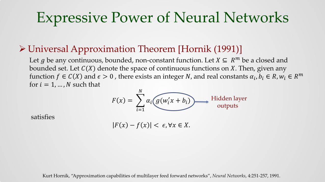
Universal Approximation Theorem [Hornik (1991)]Let 𝑔𝑔 be any continuous, bounded, non-constant function. Let 𝑋𝑋 ⊆ 𝑅𝑅𝑚𝑚 be a closed and bounded set. Let 𝐶𝐶(𝑋𝑋) denote the space of continuous functions on 𝑋𝑋. Then, given any function 𝑓𝑓 ∈ 𝐶𝐶 𝑋𝑋 and 𝜖𝜖 > 0 , there exists an integer 𝑁𝑁, and real constants 𝛼𝛼𝑖𝑖 , 𝑏𝑏𝑖𝑖 ∈ 𝑅𝑅,𝑤𝑤𝑖𝑖 ∈ 𝑅𝑅𝑚𝑚for 𝑖𝑖 = 1, … ,𝑁𝑁 such that

𝐹𝐹 𝑥𝑥 = �𝑖𝑖=1

𝑁𝑁

𝛼𝛼𝑖𝑖 𝑔𝑔(𝑤𝑤𝑖𝑖′𝑥𝑥 + 𝑏𝑏𝑖𝑖)

satisfies𝐹𝐹 𝑥𝑥 − 𝑓𝑓 𝑥𝑥 < 𝜖𝜖,∀𝑥𝑥 ∈ 𝑋𝑋.

Kurt Hornik, “Approximation capabilities of multilayer feed forward networks”, Neural Networks, 4:251-257, 1991.

Hidden layer outputs

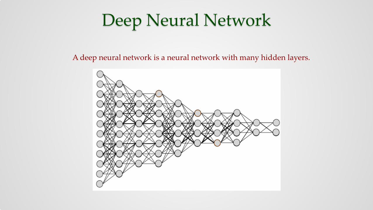
Deep Neural Network

A deep neural network is a neural network with many hidden layers.

Why Deep Networks?

Universal approximation theorem says that one hidden layer is enough to represent any continuous function. Then why deep networks??

Why Deep Networks?

Functions that can be compactly (number of computational units polynomial in the number of inputs) represented by a depth k architecture might require an exponentially large number of computational units in order to be represented by a shallower (depth < k) architecture.

Computational efficiency

In other words, for the same number of computational units, deep architectures have more expressive power than shallow architectures.

Why Deep Networks?

T. Serre, G. Kreiman, M. Kouh, C. Cadieu, U. Knoblich, and T. Poggio, “A quantitative theory of immediate visual recognition,” Progress in Brain Research, Computational Neuroscience: Theoretical Insights into Brain Function, vol. 165, pp. 33–56, 2007.

Visual cortex is organized in a deep architecture (with 5-10 levels) with a given input percept represented at multiple levels of abstraction, each level corresponding to a different area of cortex. [Serre 2007]

Biological motivation

Training Deep Neural Networks Prior to 2006, the standard approach to train a neural network was to use gradient based

techniques starting from a random initialization.

Researches have reported positive experimental results with typically one or two hidden layers, but supervised training of deeper networks using random initialization consistently yielded poor results (except for convolutional neural networks).

Why is training deep neural networks difficult?

Training Deep Neural Networks

Lack of sufficient labeled data Deep neural networks represent very complex data transformations. Supervised training of such complex models requires a large number of labeled training

samples.

Local optima Supervised training of deep networks involves optimizing a cost function that is highly

non-convex in its parameters. Gradient based approaches with random initialization usually converge to a very poor

local minima.

Training Deep Neural Networks

Diffusion of gradients The gradients that are propagated backwards rapidly diminish in magnitude as the

depth of the network increases.

The weights of the earlier layers change very slowly and the earlier layers fail to learn well.

When earlier layers do not learn well, a deep network is equivalent to a shallow network (consisting of top layers) on corrupted input (output of the bad earlier layers), and hence may perform badly compared to a shallow network on original input.

Training Deep Neural Networks

What to do??

Training Deep Neural Networks

Lots of free unlabeled data on internet these days!!

Can we use unlabeled data to train deep networks?

Unsupervised Layer-wise Pre-training In 2006, Hinton et. al. introduced an unsupervised training approach known as pre-training.

The main idea of pre-training is to train the layers of the network one at a time, in an unsupervised manner.

Various unsupervised pre-training approaches have been proposed in the recent past based on restricted Boltzmann machines [Hinton 2006], autoencoders [Bengio 2006], sparse autoencoders [Ranzato 2006], denoising autoencoders [Vincent 2008], etc.

After unsupervised training of each layer, the learned weights are used for initialization and the entire deep network is fine-tuned in a supervised manner using the labeled training data.

G. E. Hinton, S. Osindero, and Y. Teh, “A fast learning algorithm for deep belief nets,” Neural Computation, vol. 18, pp. 1527–1554, 2006.

Y. Bengio, P. Lamblin, D. Popovici, and H. Larochelle, “Greedy layer-wise training of deep networks,” NIPS, 2006.

M. Ranzato, C. Poultney, S. Chopra, and Y. LeCun, “Efficient learning of sparse representations with an energy-based model,” NIPS, 2006.

P. Vincent, H. Larochelle, Y. Bengio, and P.-A. Manzagol, “Extracting and composing robust features with denoising autoencoders,” ICML, 2008.

Unsupervised Layer-wise Pre-training

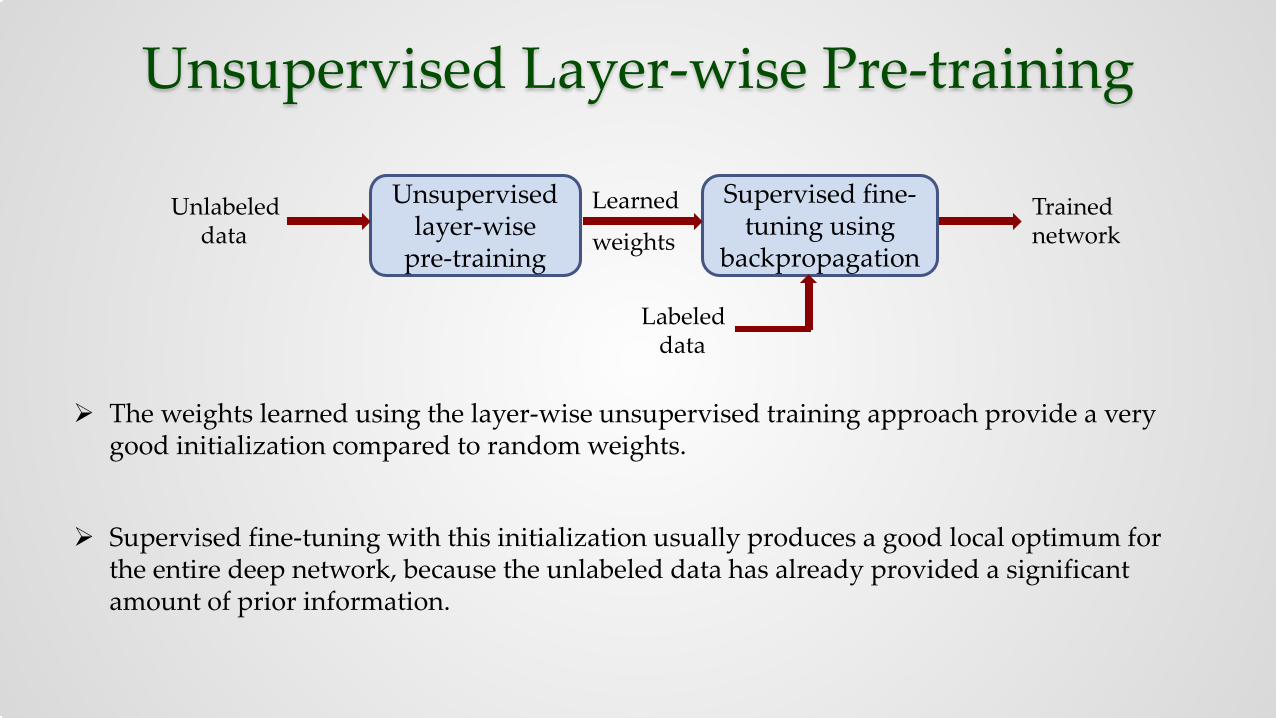
The weights learned using the layer-wise unsupervised training approach provide a very good initialization compared to random weights.

Supervised fine-tuning with this initialization usually produces a good local optimum for the entire deep network, because the unlabeled data has already provided a significant amount of prior information.

Unsupervised layer-wise

pre-training

Supervised fine-tuning using

backpropagation

Labeled data

Learned

weightsUnlabeled

dataTrained network

Convolutional Neural Networks (CNNs)

Fully connectedLocal connections with

different weights

Local connections sharing the weights Convolutional layer

Multiple convolutions using different filters

Image credit: CVPR12 Tutorial on deep learning

Equivalent to convolution by a filter

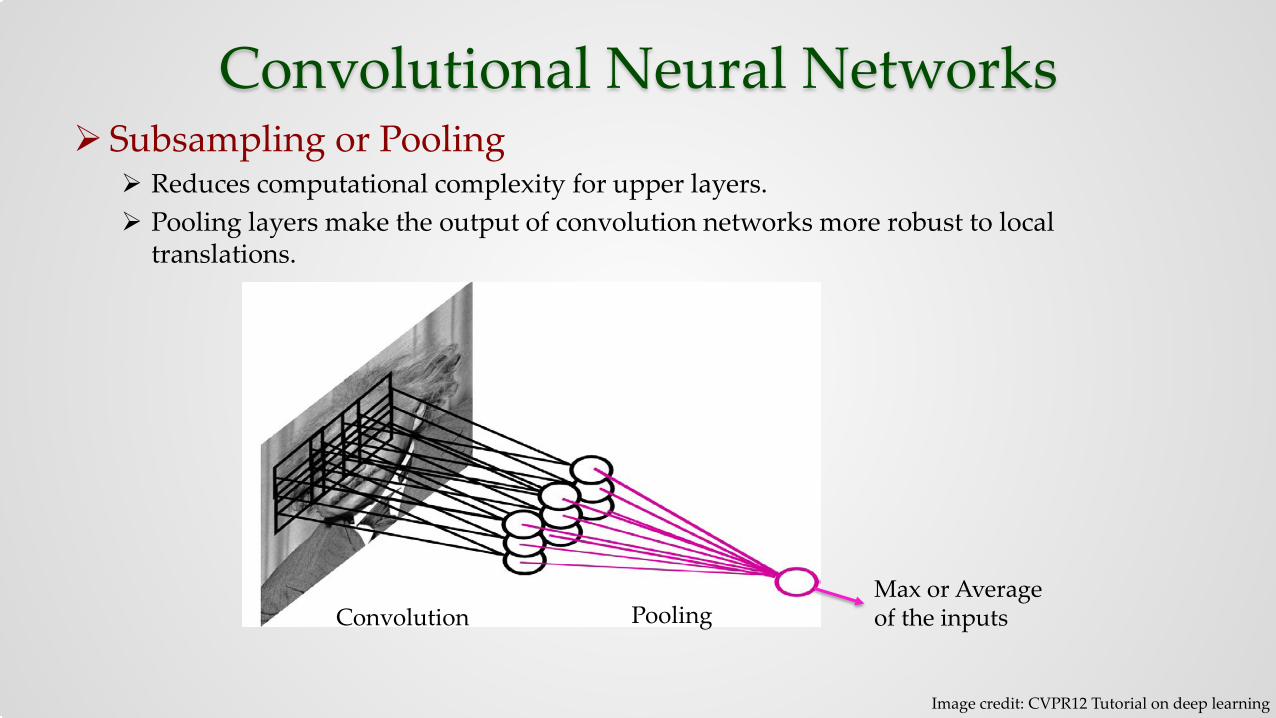
Convolutional Neural Networks Subsampling or Pooling

Reduces computational complexity for upper layers. Pooling layers make the output of convolution networks more robust to local

translations.

Convolution Pooling Max or Average of the inputs

Image credit: CVPR12 Tutorial on deep learning

Convolutional Neural Networks CNNs were inspired by the visual system’s architecture.

Modern understanding of the functioning of the visual system is consistent with the processing style found in CNNs [Serre 2007].

LeNet architecture used for character/digit recognition [LeCun 1998].

T. Serre, G. Kreiman, M. Kouh, C. Cadieu, U. Knoblich, and T. Poggio, “A quantitative theory of immediate visual recognition,” Progress in Brain Research, Computational Neuroscience: Theoretical Insights into Brain Function, vol. 165, pp. 33–56, 2007.

Training Deep CNNs Supervised training of deep neural networks always yielded poor results except for CNNs.

Long before 2006, researchers were successful in supervised training of deep CNNs (5-6 hidden layers) without any pre-training.

The small fan-in of the neurons in a CNN could be helping the gradients to propagate through many layers without diffusing so much as to become useless.

The local connectivity structure is a very strong prior that is particularly appropriate for vision tasks, and sets the parameters of the whole network in a favorable region (with all non-connections corresponding to zero weight) from which gradient based optimization works well.

What makes CNNs easier to train?

Unsupervised Pre-training

Pre-training

Unsupervised approaches Restricted Boltzmann machines (RBM) Autoencoders (AE) Sparse autoencoders (SAE) Denoising autoencoders (DAE)

In this talk we will focus on autoencoders and denoising autoencoders.

Unsupervised layer-wise

pre-training

Supervised fine-tuning using

backpropagation

Labeled data

Learned

weightsUnlabeled

dataTrained network

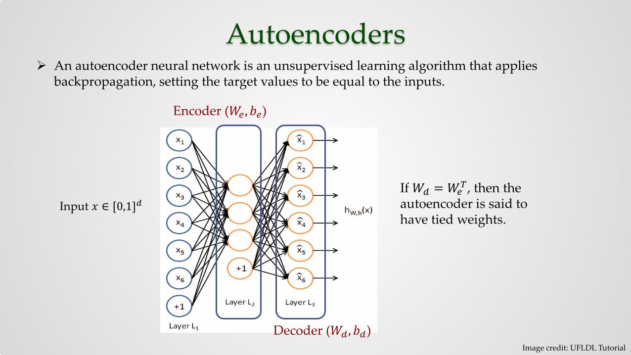
Autoencoders An autoencoder neural network is an unsupervised learning algorithm that applies

backpropagation, setting the target values to be equal to the inputs.

Image credit: UFLDL Tutorial

Encoder (𝑊𝑊𝑒𝑒 ,𝑏𝑏𝑒𝑒)

Decoder (𝑊𝑊𝑑𝑑 ,𝑏𝑏𝑑𝑑)

If 𝑊𝑊𝑑𝑑 = 𝑊𝑊𝑒𝑒𝑇𝑇, then the

autoencoder is said to have tied weights.

Input 𝑥𝑥 ∈ [0,1]𝑑𝑑

Autoencoders

Autoencoders are trained using backpropagation.

Two common cost functions

�𝑖𝑖=1

𝑁𝑁

�𝑥𝑥𝑖𝑖 − 𝑥𝑥𝑖𝑖 22

�𝑖𝑖=1

𝑁𝑁

�𝑗𝑗=1

𝑑𝑑

𝑥𝑥𝑖𝑖𝑗𝑗 log �𝑥𝑥𝑖𝑖

𝑗𝑗 − 1 − 𝑥𝑥𝑖𝑖𝑗𝑗 log 1 − �𝑥𝑥𝑖𝑖

𝑗𝑗In the case of binary inputs:

In the case of real-valued inputs:

Encoder𝑓𝑓

Decoderℎ

𝑥𝑥 �𝑥𝑥 = ℎ 𝑓𝑓 𝑥𝑥 = 𝑔𝑔(𝑊𝑊𝑑𝑑𝑓𝑓(𝑥𝑥) + 𝑏𝑏𝑑𝑑)𝑓𝑓 𝑥𝑥 = 𝑔𝑔 𝑊𝑊𝑒𝑒𝑥𝑥 + 𝑏𝑏𝑒𝑒

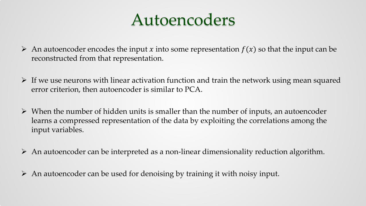
Autoencoders An autoencoder encodes the input 𝑥𝑥 into some representation 𝑓𝑓(𝑥𝑥) so that the input can be

reconstructed from that representation.

If we use neurons with linear activation function and train the network using mean squared error criterion, then autoencoder is similar to PCA.

When the number of hidden units is smaller than the number of inputs, an autoencoder learns a compressed representation of the data by exploiting the correlations among the input variables.

An autoencoder can be interpreted as a non-linear dimensionality reduction algorithm.

An autoencoder can be used for denoising by training it with noisy input.

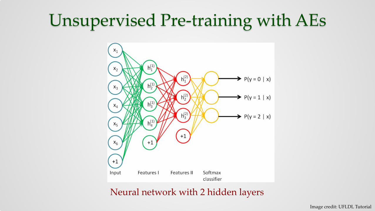
Unsupervised Pre-training with AEs

Neural network with 2 hidden layersImage credit: UFLDL Tutorial

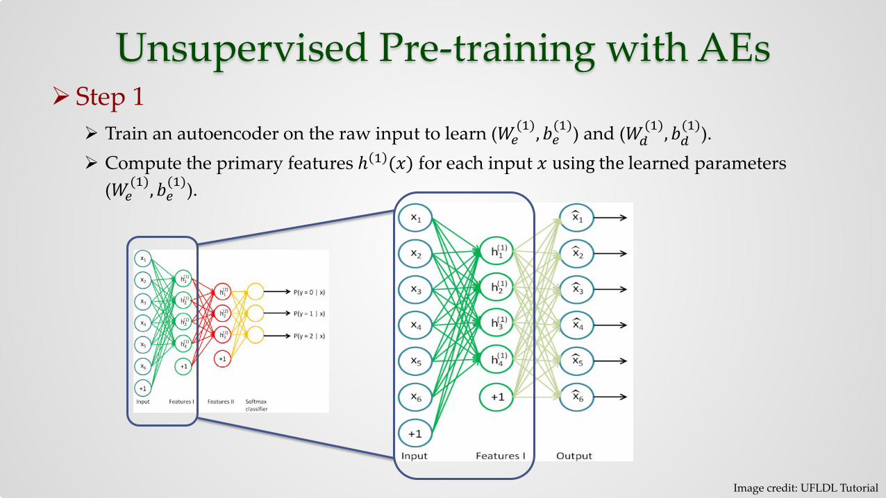
Unsupervised Pre-training with AEs Step 1

Train an autoencoder on the raw input to learn (𝑊𝑊𝑒𝑒(1),𝑏𝑏𝑒𝑒

(1)) and (𝑊𝑊𝑑𝑑(1),𝑏𝑏𝑑𝑑

(1)). Compute the primary features ℎ 1 (𝑥𝑥) for each input 𝑥𝑥 using the learned parameters

(𝑊𝑊𝑒𝑒(1),𝑏𝑏𝑒𝑒

(1)).

Image credit: UFLDL Tutorial

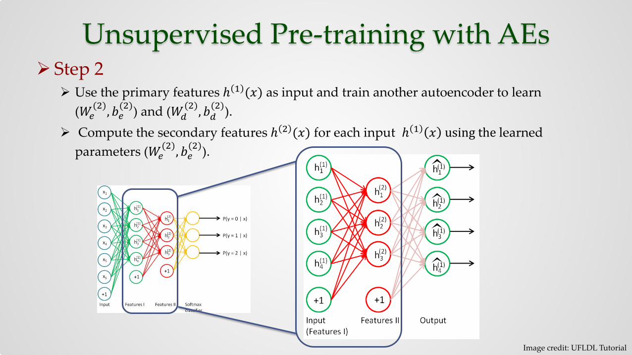
Unsupervised Pre-training with AEs Step 2

Use the primary features ℎ 1 (𝑥𝑥) as input and train another autoencoder to learn (𝑊𝑊𝑒𝑒

(2),𝑏𝑏𝑒𝑒(2)) and (𝑊𝑊𝑑𝑑

(2),𝑏𝑏𝑑𝑑(2)).

Compute the secondary features ℎ 2 (𝑥𝑥) for each input ℎ 1 𝑥𝑥 using the learned parameters (𝑊𝑊𝑒𝑒

(2),𝑏𝑏𝑒𝑒(2)).

Image credit: UFLDL Tutorial

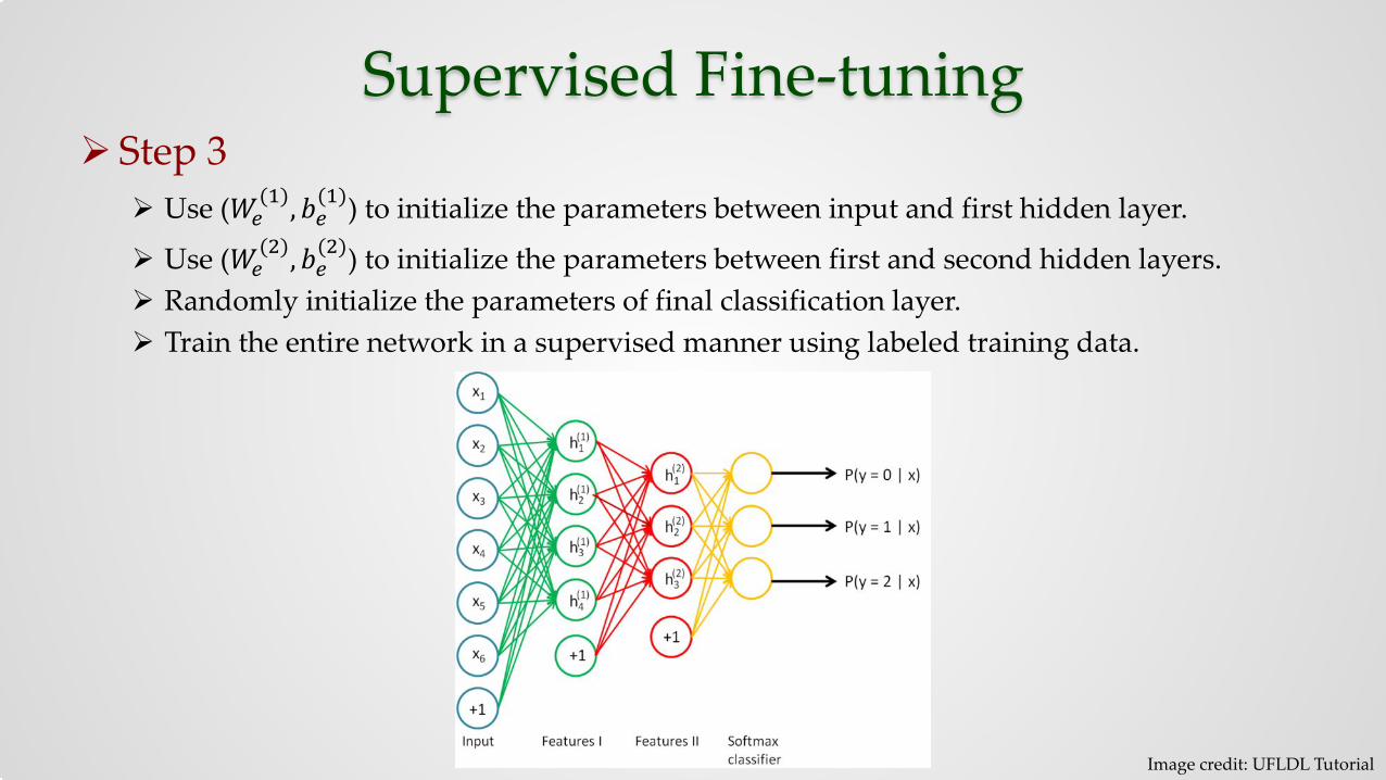
Supervised Fine-tuning Step 3

Use (𝑊𝑊𝑒𝑒(1),𝑏𝑏𝑒𝑒

(1)) to initialize the parameters between input and first hidden layer.

Use (𝑊𝑊𝑒𝑒(2),𝑏𝑏𝑒𝑒

(2)) to initialize the parameters between first and second hidden layers. Randomly initialize the parameters of final classification layer. Train the entire network in a supervised manner using labeled training data.

Image credit: UFLDL Tutorial

Denoising Autoencoders A denoising autoencoder is nothing but an autoencoder trained to reconstruct a clean input

from a corrupted one.

Motivation Humans can recognize patterns from partially occluded or corrupted data. A good representation should be robust to partial destruction of the data.

Corrupt the input 𝑥𝑥 to get a partially destroyed version �𝑥𝑥 by means of some stochastic mapping �𝑥𝑥 ~ 𝑞𝑞( �𝑥𝑥|𝑥𝑥) and train an autoencoder to recover 𝑥𝑥 from �𝑥𝑥.

Pre-training deep networks using denoising autoencoders was shown to work better than pre-training using ordinary autoencoders on MNIST digit dataset when images were corrupted by randomly choosing some of the pixels and setting their values to zero.

Thank You

Yaniv Taigman, Ming Yang, Marc’Aurelio Ranzato and Lior Wolf, “DeepFace: Closing the Gap to Human-Level performance in Face Verification”, CVPR 2014.