Embed Size (px)
Citation preview

Introduction to Computer Control SystemsLecture 7: LTI system stability
Dave Zachariah
Div. Systems and Control, Dept. Information Technology,Uppsala University
December 9, 2014
(UU/Info Technology/SysCon) Intro. Computer Control Sys. December 9, 2014 1 / 1
Today’s lecture: What and why?
BIBO stabilityWhy: If system is unstable, controller becomes critical
Nyquist stability criterionWhy: Will the controller stabilize or destabilize closed-loop system?Local stability of nonlinear systemsWhy: Many real systems are really nonlinear
(UU/Info Technology/SysCon) Intro. Computer Control Sys. December 9, 2014 2 / 1
Today’s lecture: What and why?
BIBO stabilityWhy: If system is unstable, controller becomes criticalNyquist stability criterionWhy: Will the controller stabilize or destabilize closed-loop system?
Local stability of nonlinear systemsWhy: Many real systems are really nonlinear
(UU/Info Technology/SysCon) Intro. Computer Control Sys. December 9, 2014 2 / 1
Today’s lecture: What and why?
BIBO stabilityWhy: If system is unstable, controller becomes criticalNyquist stability criterionWhy: Will the controller stabilize or destabilize closed-loop system?Local stability of nonlinear systemsWhy: Many real systems are really nonlinear
(UU/Info Technology/SysCon) Intro. Computer Control Sys. December 9, 2014 2 / 1
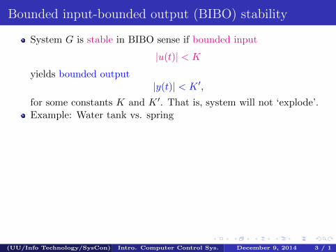
Bounded input-bounded output (BIBO) stability
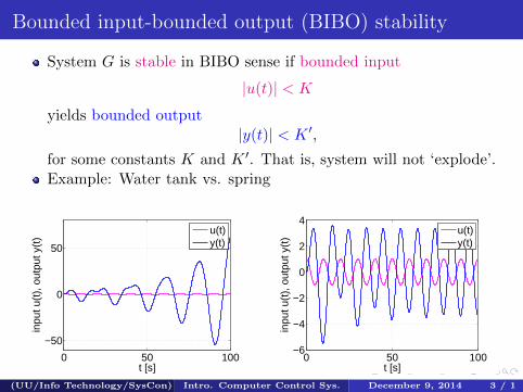
System G is stable in BIBO sense if bounded input
|u(t)| < K
yields bounded output|y(t)| < K ′,
for some constants K and K ′. That is, system will not ‘explode’.Example: Water tank vs. spring
0 50 100
−50
0
50
t [s]
inpu
t u(t
), o
utpu
t y(t
)
u(t)y(t)
0 50 100−6
−4
−2
0
2
4
t [s]
inpu
t u(t
), o
utpu
t y(t
)
u(t)y(t)
(UU/Info Technology/SysCon) Intro. Computer Control Sys. December 9, 2014 3 / 1
Bounded input-bounded output (BIBO) stability
System G is stable in BIBO sense if bounded input
|u(t)| < K
yields bounded output|y(t)| < K ′,
for some constants K and K ′. That is, system will not ‘explode’.Example: Water tank vs. spring
0 50 100
−50
0
50
t [s]
inpu
t u(t
), o
utpu
t y(t
)
u(t)y(t)
0 50 100−6
−4
−2
0
2
4
t [s]
inpu
t u(t
), o
utpu
t y(t
)
u(t)y(t)
(UU/Info Technology/SysCon) Intro. Computer Control Sys. December 9, 2014 3 / 1
Bounded input-bounded output (BIBO) stability, cont’d
For LTI systems we have y(t) =∫ tτ=0 g(τ)u(t− τ)dτ .
Then
|y(t)| ≤∫ t
τ=0|g(τ)||u(t− τ)|dτ ≤
∫ t
τ=0|g(τ)|Kdτ
Using partial fraction of transfer function
G(s) =n∑i=1
αisi − pi
⇒ g(τ) = L−1{G(s)} =n∑i=1
α′iepiτ
where pi are the poles.
(UU/Info Technology/SysCon) Intro. Computer Control Sys. December 9, 2014 4 / 1
Bounded input-bounded output (BIBO) stability, cont’d
For LTI systems we have y(t) =∫ tτ=0 g(τ)u(t− τ)dτ . Then
|y(t)| ≤∫ t
τ=0|g(τ)||u(t− τ)|dτ ≤
∫ t
τ=0|g(τ)|Kdτ
Using partial fraction of transfer function
G(s) =
n∑i=1
αisi − pi
⇒ g(τ) = L−1{G(s)} =
n∑i=1
α′iepiτ
where pi are the poles.
(UU/Info Technology/SysCon) Intro. Computer Control Sys. December 9, 2014 4 / 1
Bounded input-bounded output (BIBO) stability, cont’d
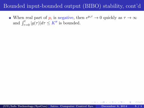
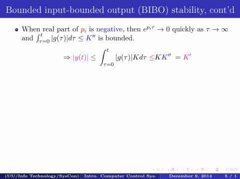
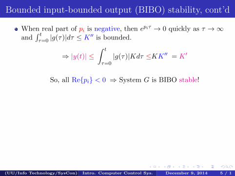
When real part of pi is negative, then epiτ → 0 quickly as τ →∞and
∫ tτ=0 |g(τ)|dτ ≤ K ′′ is bounded.
⇒ |y(t)| ≤∫ t
τ=0|g(τ)|Kdτ ≤KK ′′ = K ′
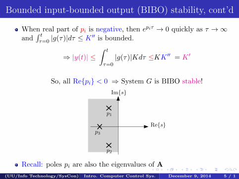
So, all Re{pi} < 0 ⇒ System G is BIBO stable!
Re{s}
Im{s}
p3
p1
p2
Recall: poles pi are also the eigenvalues of A
(UU/Info Technology/SysCon) Intro. Computer Control Sys. December 9, 2014 5 / 1
Bounded input-bounded output (BIBO) stability, cont’d
When real part of pi is negative, then epiτ → 0 quickly as τ →∞and
∫ tτ=0 |g(τ)|dτ ≤ K ′′ is bounded.
⇒ |y(t)| ≤∫ t
τ=0|g(τ)|Kdτ ≤KK ′′ = K ′
So, all Re{pi} < 0 ⇒ System G is BIBO stable!
Re{s}
Im{s}
p3
p1
p2
Recall: poles pi are also the eigenvalues of A
(UU/Info Technology/SysCon) Intro. Computer Control Sys. December 9, 2014 5 / 1
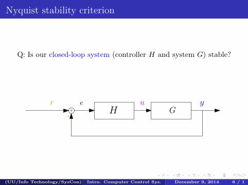
Nyquist stability criterion
Q: Is our closed-loop system (controller H and system G) stable?
yur+
−G
eH
(UU/Info Technology/SysCon) Intro. Computer Control Sys. December 9, 2014 6 / 1
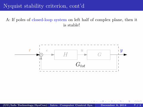
Nyquist stability criterion, cont’d
A: If poles of closed-loop system on left half of complex plane, then itis stable!
yur+
−G
eH
Gtot
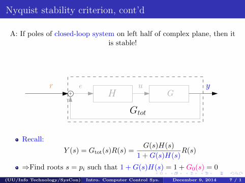
Recall:
Y (s) = Gtot(s)R(s) =G(s)H(s)
1 +G(s)H(s)R(s)
⇒Find roots s = pi such that 1 +G(s)H(s) = 1 +G0(s) = 0
(UU/Info Technology/SysCon) Intro. Computer Control Sys. December 9, 2014 7 / 1
Nyquist stability criterion, cont’d
A: If poles of closed-loop system on left half of complex plane, then itis stable!
yur+
−G
eH
Gtot
Recall:
Y (s) = Gtot(s)R(s) =G(s)H(s)
1 +G(s)H(s)R(s)
⇒Find roots s = pi such that 1 +G(s)H(s) = 1 +G0(s) = 0
(UU/Info Technology/SysCon) Intro. Computer Control Sys. December 9, 2014 7 / 1
Nyquist stability criterion, cont’d
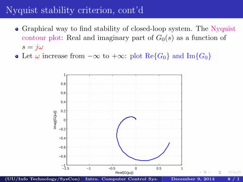
Graphical way to find stability of closed-loop system. The Nyquistcontour plot: Real and imaginary part of G0(s) as a function ofs = jω
Let ω increase from −∞ to +∞: plot Re{G0} and Im{G0}
(UU/Info Technology/SysCon) Intro. Computer Control Sys. December 9, 2014 8 / 1
Nyquist stability criterion, cont’d
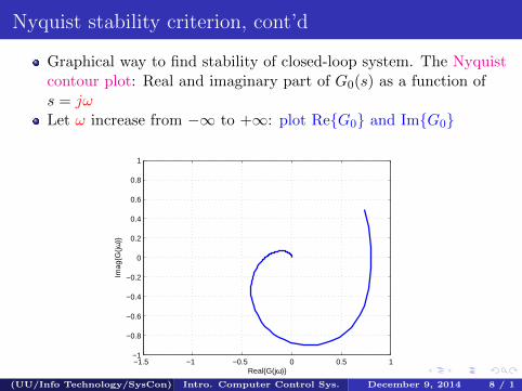
Graphical way to find stability of closed-loop system. The Nyquistcontour plot: Real and imaginary part of G0(s) as a function ofs = jωLet ω increase from −∞ to +∞: plot Re{G0} and Im{G0}
−1.5 −1 −0.5 0 0.5 1−1
−0.8
−0.6
−0.4
−0.2
0
0.2
0.4
0.6
0.8
1
Real{G(jω)}
Imag
{G(jω
)}
(UU/Info Technology/SysCon) Intro. Computer Control Sys. December 9, 2014 8 / 1
Nyquist stability criterion, cont’d
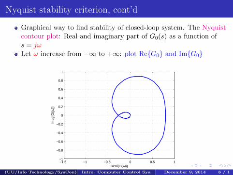
Graphical way to find stability of closed-loop system. The Nyquistcontour plot: Real and imaginary part of G0(s) as a function ofs = jωLet ω increase from −∞ to +∞: plot Re{G0} and Im{G0}
−1.5 −1 −0.5 0 0.5 1−1
−0.8
−0.6
−0.4
−0.2
0
0.2
0.4
0.6
0.8
1
Real{G(jω)}
Imag
{G(jω
)}
(UU/Info Technology/SysCon) Intro. Computer Control Sys. December 9, 2014 8 / 1
Nyquist stability criterion, cont’d
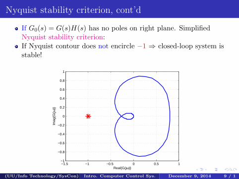
If G0(s) = G(s)H(s) has no poles on right plane. SimplifiedNyquist stability criterion:If Nyquist contour does not encircle −1 ⇒ closed-loop system isstable!
−1.5 −1 −0.5 0 0.5 1−1
−0.8
−0.6
−0.4
−0.2
0
0.2
0.4
0.6
0.8
1
Real{G(jω)}
Imag
{G(jω
)}
(UU/Info Technology/SysCon) Intro. Computer Control Sys. December 9, 2014 9 / 1
Example of graphical test
System and controller with tuning parameter K > 0:
G(s) =1
s(s+ 2)H(s) =
K
s+ 1
Changing K moves poles of closed-loop system Gtot! When is itstable? On the board
Note: G0(s) = G(s)H(s) has no poles on right plane ⇒ we can usesimplified Nyquist criterion.
(UU/Info Technology/SysCon) Intro. Computer Control Sys. December 9, 2014 10 / 1
Example of graphical test
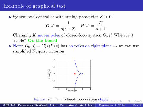
System and controller with tuning parameter K > 0:
G(s) =1
s(s+ 2)H(s) =
K
s+ 1
Changing K moves poles of closed-loop system Gtot! When is itstable? On the boardNote: G0(s) = G(s)H(s) has no poles on right plane ⇒ we can usesimplified Nyquist criterion.
−3 −2 −1 0 1−1
−0.5
0
0.5
1
Real{G0(jω)}
Imag
{G0(jω
)}
Figure: K = 2 ⇒ closed-loop system stable!
(UU/Info Technology/SysCon) Intro. Computer Control Sys. December 9, 2014 10 / 1
Example of graphical test
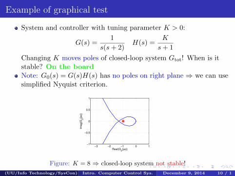
System and controller with tuning parameter K > 0:
G(s) =1
s(s+ 2)H(s) =
K
s+ 1
Changing K moves poles of closed-loop system Gtot! When is itstable? On the boardNote: G0(s) = G(s)H(s) has no poles on right plane ⇒ we can usesimplified Nyquist criterion.
−3 −2 −1 0 1−1
−0.5
0
0.5
1
Real{G0(jω)}
Ima
g{G
0(j
ω)}
Figure: K = 8 ⇒ closed-loop system not stable!
(UU/Info Technology/SysCon) Intro. Computer Control Sys. December 9, 2014 10 / 1
Stability of nonlinear systems?
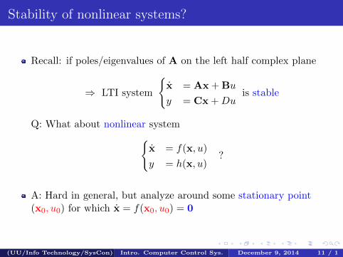
Recall: if poles/eigenvalues of A on the left half complex plane
⇒ LTI system
{x = Ax + Bu
y = Cx +Duis stable
Q: What about nonlinear system{x = f(x, u)
y = h(x, u)?
A: Hard in general, but analyze around some stationary point(x0, u0) for which x = f(x0, u0) = 0
(UU/Info Technology/SysCon) Intro. Computer Control Sys. December 9, 2014 11 / 1
Stability of nonlinear systems?
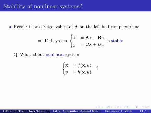
Recall: if poles/eigenvalues of A on the left half complex plane
⇒ LTI system
{x = Ax + Bu
y = Cx +Duis stable
Q: What about nonlinear system{x = f(x, u)
y = h(x, u)?
A: Hard in general, but analyze around some stationary point(x0, u0) for which x = f(x0, u0) = 0
(UU/Info Technology/SysCon) Intro. Computer Control Sys. December 9, 2014 11 / 1
Stability of nonlinear systems? Cont’d
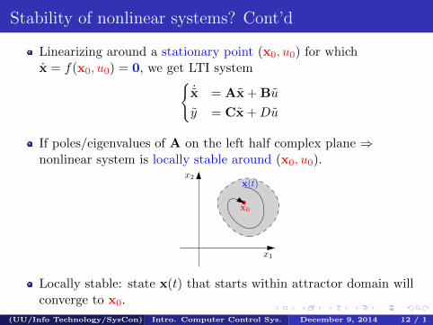
Linearizing around a stationary point (x0, u0) for whichx = f(x0, u0) = 0, we get LTI system{
˙x = Ax + Bu
y = Cx +Du
If poles/eigenvalues of A on the left half complex plane ⇒nonlinear system is locally stable around (x0, u0).
x1
x2
x0
x(t)
Locally stable: state x(t) that starts within attractor domain willconverge to x0.
(UU/Info Technology/SysCon) Intro. Computer Control Sys. December 9, 2014 12 / 1
Stability of nonlinear systems? Cont’d
Linearizing around a stationary point (x0, u0) for whichx = f(x0, u0) = 0, we get LTI system{
˙x = Ax + Bu
y = Cx +Du
If poles/eigenvalues of A on the left half complex plane ⇒nonlinear system is locally stable around (x0, u0).
x1
x2
x0
x(t)
Locally stable: state x(t) that starts within attractor domain willconverge to x0.
(UU/Info Technology/SysCon) Intro. Computer Control Sys. December 9, 2014 12 / 1
Today’s lecture: What and why?
BIBO stabilityWhy: If system is unstable, controller becomes criticalNyquist stability criterionWhy: Will the controller stabilize or destabilize closed-loop system?Local stability of nonlinear systemsWhy: Many real systems are really nonlinear
(UU/Info Technology/SysCon) Intro. Computer Control Sys. December 9, 2014 13 / 1