Introduction to Business Statistics Chapter 5 Discrete ... 5 2.pdf · Discrete random variables and their probability distribution ... that x assumes a value in the interval 2 to

DEPARTMENT OF QUANTITATIVE METHODS & INFORMATION SYSTEMS

Introduction to Business StatisticsQM 120

Chapter 5

Discrete random variables and their probability distribution distribution

Dr. Mohammad ZainalSpring 2008

Chapter 5: Random Variables2

Random variables

2

# of PC’s owned Frequency Relative Frequency

0 120 .12

1 180 .18

2 470 .47

3 230 233 230 .23

N = 1000 Sum = 1.000

Let x denote the number of PCs owned by a family. Then x

can take any of the four possible values (0, 1, 2, and 3).

A random variable (RV) is a variable whose value is

determined by the outcome of a random experiment.y p

3


Discrete random variable

A random variable that assumes countable values is called a

discrete random variable.

Examples of discrete RVs:

Number of cars sold at a dealership during a week

Number of houses in a certain block

Number of fish caught on a fishing tripg g p

Number of costumers in a bank at any given day

Continuous random variableContinuous random variable

A random variable that can assume any value contained in

one or more intervals is called a continuous random variable.one or more intervals is called a continuous random variable.

4


Examples of continuous RVs:Height of a personHeight of a person

Time taken to complete a test

Weight of a fishg

Price of a car

E l Cl if h f h f ll i RV diExample: Classify each of the following RVs as discrete or

continuous.

Th b f t d t b k d i kThe number of new accounts opened at a bank during a week

The time taken to run a marathon

The price of a meal in fast food restaurantThe price of a meal in fast food restaurant

The score of a football game

The weight of a parcel

5

Chapter 5: Probability Distribution of a Discrete RV5

The probability distribution of a discrete RV lists all the

bl l h h RV d hpossible value that the RV can assume and their

corresponding probabilities.

Example: Write the probability distribution of the number of

PCs owned by a family.

# of PC’s owned

Frequency Relative Frequencyowned Frequency

0 120 .12

1 180 .18

2 470 .47

3 230 .23

N 1000 S 1 000N = 1000 Sum = 1.000

6


The following two characteristics must hold for any discrete

b b l d bprobability distribution:

The probability assigned to each value of a RV x lies in the range 0to 1; that is 0 ≤ P(x) ≤ 1 for each x.to 1; that is 0 ≤ P(x) ≤ 1 for each x.

The sum of the probabilities assigned to all possible values of x isequal to 1.0; that is ΣP(x) = 1.

Example: Each of the following tables lists certain values of xand their probabilities. Determine whether or not each tablerepresents a valid probability distribution.

x P(x) x P(x) x P(x)

0 .08

1 .11

2 39

0 .25

1 .34

2 28

4 .2

5 .3

6 62 .39

3 .27

2 .28

3 .13

6 .6

8 ‐.1

7


Example: The following table lists the probability distribution of

a discrete RV x.

6543210x

a) P( 3) b) P( ≤ 2) ) P( ≥ 4) d) P(1 ≤ ≤ 4)

.06.09.12.15.28.19.11P(x)

a) P(x = 3) b) P(x ≤ 2) c) P(x ≥ 4) d) P(1 ≤ x ≤ 4)e) Probability that x assumes a value less than 4

f) Probability that x assumes a value greater than 2f) Probability that x assumes a value greater than 2

g) Probability that x assumes a value in the interval 2 to 5

8


Example: For the following table

54321

a) Construct a probability distribution table. Draw a graph of

54321x

121624208P(x)

a) Construct a probability distribution table. Draw a graph of the probability distribution.

b) Find the following probabilitiesi. P(x = 3) ii. P(x < 4) iii. P(x ≥ 3) iv. P(2 ≤ x ≤ 4)

9

Chapter 5: Mean of a discrete RV9

Mean of a discrete RV

The mean μ ‐or expected value E(x)‐ of a discrete RV is thevalue that you would expect to observe on average if the

i t i t d i d iexperiment is repeated again and again

It is denoted by ( ) ( )E x xp x=∑

Illustration: Let us toss two fair coins, and let x denote thenumber of heads observed We should have the following

( ) ( )E x xp x=∑

number of heads observed. We should have the followingprobability distribution table

210x

Suppose we repeat the experiment a large number of times,say n =4 000 We should expect to have approximately

1/41/21/4P(x)

say n =4,000. We should expect to have approximately

10


1 thousand zeros, 2 thousand ones, and 1 thousand twos. Then th l f ld lthe average value of x would equal

Sum of measurements 1,000(0) 2,000(1) 1000(2)

4 000

+ +=

4,000

1 1 1 (0) (1) (2)

4 4

2

n

⎛ ⎞ ⎛ ⎞ ⎛ ⎞= + +⎜ ⎟ ⎜ ⎟ ⎜ ⎟⎝ ⎠ ⎝ ⎠ ⎝ ⎠

Similarly, if we use the , we would have

⎝ ⎠ ⎝ ⎠ ⎝ ⎠

( ) ( )E x xp x=∑( ) 0 (0) 1 (1) 2 (2)

0(1/ 4) 1(1/ 2) 2(1/ 4)

E x P P P= + += + +

1=

11


Example: Recall “ number of PC’s owned by a family”

l F d h b f PC d b f lexample. Find the mean number of PCs owned by a family.

12


Example: In a lottery conducted to benefit the local firecompany 8000 tickets are to be sold at $5 each The prize is acompany, 8000 tickets are to be sold at $5 each. The prize is a$12,000. If you purchase two tickets, what is your expectedgain?


Example: Determine the annual premium for a $1000insurance policy covering an event that over a long period of

13

time, has occurred at the rate of 2 times in 100. Let

x : the yearly financial gain to the insurance companyresulting from the sale of the policyresulting from the sale of the policy

C : unknown premium

Calculate the value of C such that the expected gain E(x) willCalculate the value of C such that the expected gain E(x) willequal to zero so that the company can add the administrativecosts and profit.


Example: You can insure a $50,000 diamond for its total value

by paying a premium of D dollars. If the probability of theft in

14

y p y g p p y

a given year is estimated to be .01, what premium should the

insurance company charge if it wants the expected gain to

equal $1000.

Chapter 5: Standard Deviation of a Discrete RV15

The standard deviation of a discrete RV x, denoted by σ,measures the spread of its probability distribution.

15

A higher value of σ indicates that x can assume values overa larger range about the mean. While, a smaller valueindicates that most of the values that can x assume areclustered closely around the mean.

Th d d d i i b f d i h f ll iThe standard deviation σ can be found using the followingformula:

2 2( )x p xσ μ= −∑Hence, the variance σ2 can be obtained by squaring itsstandard deviation σ

( )x p xσ μ= −∑

standard deviation σ.


Example: Recall “ number of PC’s owned by a family”example. Find the standard deviation of PCs owned by a

16

family.


Example: An electronic store sells a particular model of acomputer notebook. There are only four notebooks in stocks,

17

and the manager wonders what today’s demand for thisparticular model will be. She learns from marketingdepartment that the probability distribution for x the dailydepartment that the probability distribution for x, the dailydemand for the laptop, is as shown in the table.

54321x

Find the mean, variance, and the standard deviation of x. Is itlik l th t fi t ill t t b l t ?

.05.10.15.20.40P(x)

likely that five or more costumers will want to buy a laptop?


Example: A farmer will earn a profit of $30,000 in case ofheavy rain next year, $60,000 in case of moderate rain, and

18

$15,000 in case of little rain. A meteorologist forecasts that theprobability is .35 for heavy rain, .40 for moderate rain, and .25for little rain next year Let x be the RV that represents nextfor little rain next year. Let x be the RV that represents nextyear’s profits in thousands of dollars for this farmer. Write theprobability distribution of x. Find the mean, variance, and thestandard deviation of x.


Example: An instant lottery ticket costs $2. Out of a total of10,000 tickets printed for this lottery, 1000 tickets contain a

19

prize of $5 each. 100 tickets contain a prize of $10 each, 5tickets contain a prize of $1000 each, and 1 ticket has the prizeof $5000 Let x be the RV that denotes the net amount playerof $5000. Let x be the RV that denotes the net amount playerwins by playing this lottery. Write the probability distributionof x. Determine the mean and the standard deviation of x.


Example: Based in its analysis of future demand for itsproducts, the financial department a company has determined

20

that there is a .17 probability that the company will lose $1.2million during the next year, a .21 probability that it will lose$ 7 million a 37 probability that it will make a profit of $0 9$.7 million, a .37 probability that it will make a profit of $0.9million, and a .25 probability that it will make a profit of $2.3million.

a) Let x be a RV that denotes the profit earned by thiscompany during the next year. Write the probabilitydistribution of xdistribution of x.


b) Find the mean and standard deviation of the probability ofpart a.

21

Chapter 5: Factorials & Combinations22

Factorials

The symbol n!, reads as “n factorial,” represents the

22

y pproduct of all integers from n to 1. In other words,

n! = n(n ‐ 1)(n ‐ 2)(n ‐ 3)…3.2.1

Example: Evaluate 7!

7! = 7.6.5.4.3.2.1 = 5040

Example: Evaluate (12‐4)!

(12‐4)! = (8)! = 8.7.6.5.4.3.2.1 =40,320


Example: Evaluate (8‐8)!

(8‐8)! = (0)! = 1

23

(8 8)! (0)! 1

Example: Find the value of 8!p

By using factorial Table or your calculator.

Locate 8 in the column labeled n.

Then read the value for n! next

to 8.


Combinations

Combinations give the number of ways x elements can be

24

g yselected from n elements. The notation used to denote thetotal number of combinations is

)(nx

nxxn CC ==

It can be found using the following formula

!n

)!(!

!

xnx

nCC xn

nx −

==

Remember: n is always greater than or at least equal to x.


Example: Three members of a jury will be randomly selectedfrom five people. How many different combinations are

25

possible?


Using the table of combinations

Values of Table III in Appendix C lists the number of

26

combinations of n elements selected x at a time.

Example: Evaluate

the followings

a) 5C3b) 8C4) Cc) 9C5d) 5C5e) 5C0e) 5C0

Chapter 5: The Binomial Probability Distribution27

The most widely used discrete probability distribution.

27

It is applied to find the probability that an event will occurx times in n repetitions of an experiment (under certainconditions).

Suppose the probability that a VCR is defective at a factoryis .05. We can apply the binomial probability distribution tofi d th dd f tti tl d f ti VCR t thfind the odds of getting exactly one defective VCR out threeVCRs.


Binomial experiment

An experiment that satisfies the following four conditions is

28

p gcalled a binomial experiment.

There are n identical trials

Each trail has only two possible outcomes.

The probabilities of the two outcomes remain constant.

The trials are independentThe trials are independent.

A success does not mean that the corresponding outcome isA success does not mean that the corresponding outcome isconsidered favorable. Similarly, a failure doesnʹt necessarilyrefer to unfavorable outcome.


Example: Consider the experiment consisting of 10 tosses of acoin. Determine whether or not it is a binomial experiment.

29

Solution:


The binomial probability distribution and its formula.

The RV x that represents the number of successes in n trials

30

pfor a binomial experiment is called a binomial RV.

The probability distribution of x is called the binomialdistribution.

Consider the VCRs example. Let x be the number ofpdefective VCRs in a sample of 3, x can assume any of thevalues 0, 1, 2, 3.


For a binomial experiment, the probability of exactly xsuccesses in n trials is given by the binomial formula

31

( )

!

x n xn xP x C p q −=

where

l b f i l

!

!( )!x n xn

p qx n x

−=−

n = total number of trials,

p = probability of success,

q = probability of failure 1 – pq = probability of failure 1 – p,

x = number of successes in n trials,

n – x = number of failures in n trials


Example: Find P(2) for a binomial RV with n = 5 and p =0.1

32

Solution:


Example: Over a long period of time it has been observed thata given sniper can hit a target on a single trial with a

33

probability = .8. Suppose he fires four shots at the target.

a) What is the probability that he will hit the target exactly twotimes?

b) What is the probability that he will hit the target at leastb) What is the probability that he will hit the target at leastonce?


Example: Five percent of all VCRs manufactured by a largefactory are defective. A quality control inspector selects three

34

VCRs from the production line. What is the probability thatexactly one of these three VCRs is defective

Solution:


Example: At the Express Delivery Services (EDS), providinghigh‐quality service to its customers is the top priority of the

35

management. The company guarantees a refund of all chargesif a package is not delivered at its destination by the specifiedtime It is known from the past that despite all efforts 2% oftime. It is known from the past that despite all efforts, 2% ofthe packages mailed through this company does not arrive ontime. A corporation mailed 10 packages through EDS.

a) Find the probability that exactly 1 of these 10 packages willnot arrive on time

b) Find the probability that at most 1 of these 10 packages willnot arrive on timenot arrive on time.


Example: According to the U.S. Bureau of Labor Statistics, 56%of mothers with children under 6 years of age work outside

36

their homes. A random sample of 3 mothers with childrenunder 6 years of age is selected. Let x denote the number ofmothers who work outside their homes Write the probabilitymothers who work outside their homes. Write the probabilitydistribution of x and draw a graph of the probabilitydistribution.

Solution:


Using the table of binomial probabilities

We can use the tables of binomial probabilities (Table IV)

37

pgiven in Appendix C to calculate the required probabilities.

PP

.95….2.1.05xn

.0500….8000.9000.950001

.9500….2000.1000.05001 .9500….2000.1000.05001

.0025….6400.8100.902502

.0950….3200.1800.09501

.9025….0400.0100.00252

.0001….5120.7290.857403

.0071….3840.2430.13541

.1354….0960.0270.00712

.8574….0080.0010.00013


Example: Based on data from A peter D. Hart ResearchAssociates’ poll on consumer buying habits and attitudes, It was

38

estimated that 5% of American shoppers are status shoppers,that is, shoppers who love to buy designer labels. A randomsample of eight American shoppers is selected Using Binomialsample of eight American shoppers is selected. Using BinomialTable, answer the following:

a) Find the probability that exactly 3 shoppers are status) p y y ppshoppers.

b) Find the probability that at most 2 shoppers are statusshoppers.pp


c) Find the probability that at least 3 shoppers are statusshoppers.

39

d) Find the probability that 1 to 3 shoppers are status shoppers.

e) Let x be the number of status shoppers, Write the probabilitydistribution of x and draw a graph of this probability.


Probability of success and the shape of the binomial

distribution

40

distribution

For any number of trials n

The binomial probability distribution is symmetric if p = .5

p

.95.9….5….1.05xn

.0000.0001….0625….6561.814504 0.25

0.3

0.35

0.4

.0005.0036….2500….2916.17151

.0135.0486….3750….0486.01352

.1715.2916….2500….0036.00053 0.05

0.1

0.15

0.2

P(x

)

.8145.6561….0625….0001.000040

0 1 2 3 4

x


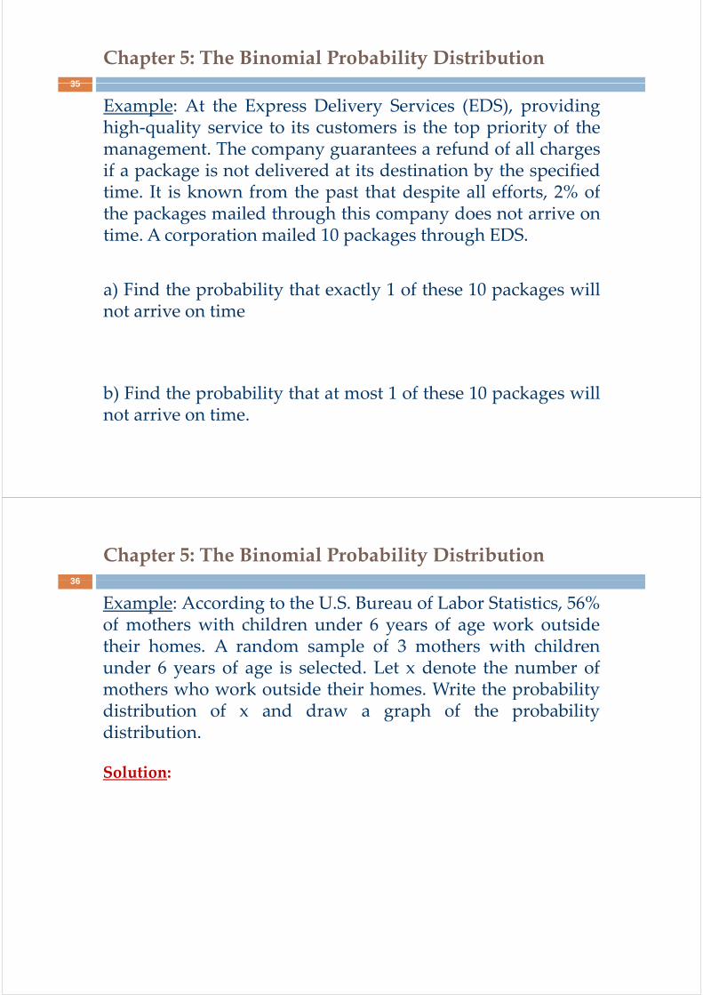
The binomial probability distribution is skewed to the right if p is less than .5

p 0.6

0.7

.95.9….5….1.05xn

.0000.0001….0625….6561.814504

.0005.0036….2500….2916.171510.2

0.3

0.4

0.5

P(x

)

.0135.0486….3750….0486.01352

.1715.2916….2500….0036.00053

.8145.6561….0625….0001.00004

0

0.1

0 1 2 3 4

x


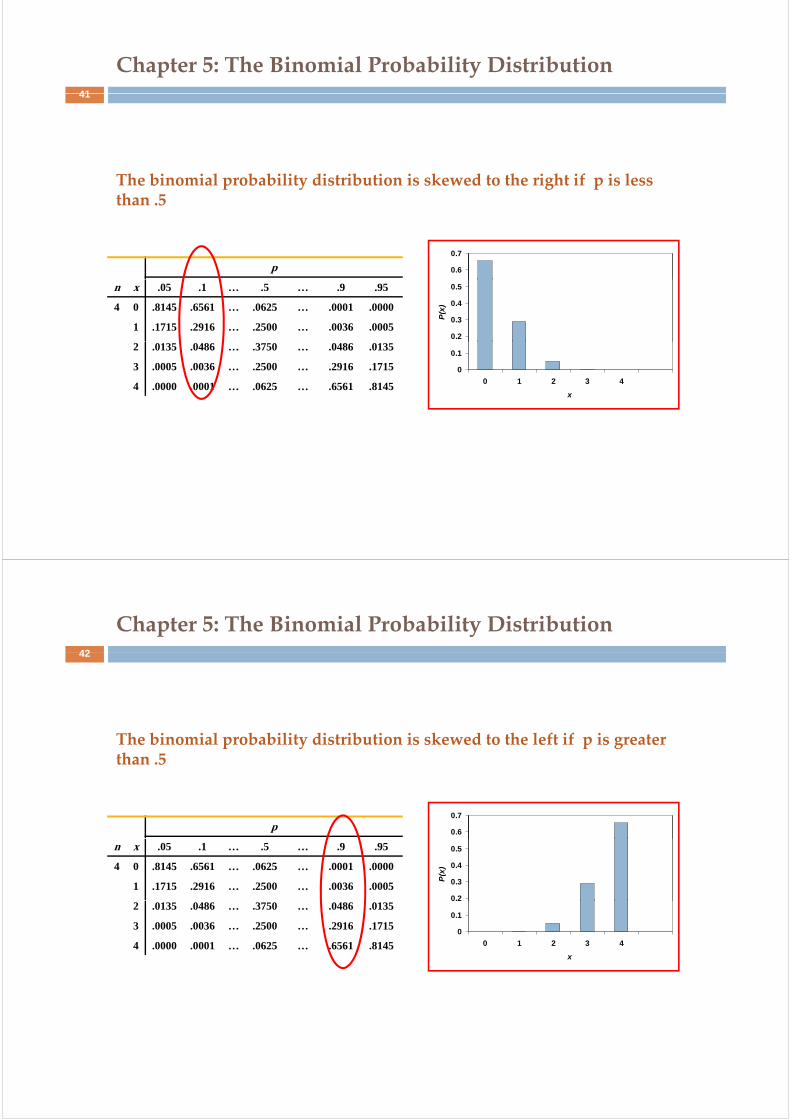
The binomial probability distribution is skewed to the left if p is greater than .5

p 0.6

0.7

.95.9….5….1.05xn

.0000.0001….0625….6561.814504

.0005.0036….2500….2916.171510.2

0.3

0.4

0.5

P(x

)

.0135.0486….3750….0486.01352

.1715.2916….2500….0036.00053

.8145.6561….0625….0001.000040

0.1

0.2

0 1 2 3 4

x


Mean and standard deviation of the binomial distribution

Although we can still use the mean and standard deviations

43

gformulas learned in 5.3 and 5.4, it is more convenient andsimpler to use the following formulas once the RV x isknown to be a binomial RVknown to be a binomial RV

and np npqμ σ= =


Example: Refer to the mothers with children under 6 years ofage example, find the mean and the standard deviation of the

44

probability distribution.

Solution:Solution:


Example: Let x be a discrete RV that posses a binomialdistribution. Using the binomial formula, find the following

45

probabilities.

f da) P(x = 5) for n = 8 and p = .6

b) P(x = 3) for n = 4 and p = .3

c) P(x = 2) for n = 6 and p = .2c) P(x 2) for n 6 and p .2

Verify your answer by using Table of Binomial Probabilities.


Example: Let x be a discrete RV that posses a binomialdistribution.

46

a) Table of Binomial Probabilities, write the probabilitydistribution for x for n = 7 and p = .3 and graph it.

b) What are the mean and the standard deviation of theprobability distribution developed in part a?


An experiment that satisfies the following four conditions iscalled a binomial experiment.

There are n identical trials

Each trail has only two possible outcomes.

The probabilities of the two outcomes remain constant.

The trials are independent.

Chapter 5: The Hypergeometric Probability Distribution48

We learned that one of the conditions required to apply thebinomial distribution is that the trials are independent so

48

the probability of the two outcomes remain constant.

What if the probability of the outcomes is not constant?

In such cases we replace the binomial distribution by thehypergeometric probability distribution.yp g p y

Such a case occurs when a sample is drawn withoutSuch a case occurs when a sample is drawn withoutreplacement from a finite population.

49

Chapter 5: The Hypergeometric Probability Distribution

Hypergeometric probability distributionLet N = total number of elements in the population

49

p pr = number of successes in the populationN – r = number of failures in the populationn = number of trials (sample size)

b f i t i lx = number of successes in n trialsn – x = number of failures in n trials

Th d th iTh b bili f The mean and the variance are given by

The probability of x successes in n trials is given by

r⎛ ⎞⎜ ⎟( ) r x N r n x

N n

C CP x

C− −=

2 r N r N n− −⎛ ⎞⎛ ⎞⎛ ⎞

nN

μ ⎛ ⎞= ⎜ ⎟⎝ ⎠

2

1

r N r N nn

N N Nσ ⎛ ⎞⎛ ⎞⎛ ⎞= ⎜ ⎟⎜ ⎟⎜ ⎟−⎝ ⎠⎝ ⎠⎝ ⎠

50


Example: Dawn corporation has 12 employees who holdmanagerial positions. Of them, 7 are female and 5 are male.

50

The company is planning to send 3 of these 12 managers to aconference. If 3 mangers are randomly selected out of 12,

a) find the probability that all 3 of them are female

51


b) find the probability that at most 1 of them is a female

51

52


Example: A case of soda has 12 bottles, 3 of which contain dietsoda. A sample of 4 bottles is randomly selected from the case

52

a) find the probability distribution of x, the number of dietsodas in the sample

53


b) what are the mean and variance of x?

53

54


Example: GESCO Insurance company has prepared a final listof 8 candidates for 2 positions. Of the 8 candidates, 5 are

54

business majors and 3 are engineers. If the company managerdecides to select randomly two candidates from this list, findthe probability thatthe probability that

a) both candidates are business majors

b) neither of the two candidates is a business major) j

c) at most one of the candidates is a business major

Chapter 5: The Poisson Probability Distribution55

The Poisson distribution is another discrete probabilitydistribution that has numerous practical applications.

55

It provides a good model for data that represent the numberof occurrence of a specified event in a given unit of time orspace.

Here are some examples of experiments for which the RV xd l d b h P i RVcan modeled by the Poisson RV:

The number of phone calls received by an operator during a day

Th b f t i l t h k t t d i hThe number of customer arrivals at checkout counter during an hour

The number of bacteria per a cm3 of a fluid

The number of machine breakdowns during a given dayThe number of machine breakdowns during a given day

The number of traffic accidents at a given time period


The Poisson probability distribution is applied toexperiments with random and independent occurrences

56

The occurrences are random in the sense they do not follow any pattern and, hence, the are unpredictable.

I d d f th t thIndependence of occurrences means that the occurrence or nonoccurrence of an event does not influence the successive occurrence of that next event.

The occurrences are always considered with respect to aninterval.

h l b l lThe interval may be a time interval, a space interval, or avolume interval.

If th b f (λ) f i i t lIf the average number of occurrences (λ) for a given intervalis known, then by using the Poisson probability we cancompute the probability of a certain number of occurrencesp p yx in that interval.


The following three conditions must be satisfied to applythe Poisson probability distribution

57

x is a discrete RV.

The occurrences are random.

The occurrences are independent.

The Poisson probability formula is given by

( )!

xeP x

x

λλ −

=

where λ (pronounced lambda) is the mean number ofoccurrences in that interval and the value of e is

i l 2 71828approximately 2.71828.


The mean number of occurrences, denoted by λ, is calledthe parameter of the Poisson probability distribution or the

58

Poisson parameter.

Remember: The interval of λ and x must be of the samelength. If they are not, the mean λ should be redefined to

k h l F i if λ i i h dmake them equal. For instance, if λ was given in hours andwe were asked to find the event in minutes, λ needs to bedivided by 60 to have both x and λ in the same intervaldivided by 60 to have both x and λ in the same intervallength


Example: The automatic teller machine (ATM) installedoutside Mansfield Savings and Loan is used on average by

59

five costumers per hour. The bank closed this ATM for onehour for repairs. What is the probability that during that houreight customers came to use this ATM?eight customers came to use this ATM?

Solution:


Example: The average number of traffic accidents on a certainsection of highway is two per week. assume that the number of

60

accidents follows a Poisson distribution with λ = 2.

1. Find the probability of no accidents on this section of highwayduring a 1‐week period.

2. Find the probability of at most three accidents on this sectionof highway during a 2‐week period.


Using the table of Poisson probabilities

The probabilities for Poisson distribution can also be found

61

pusing Poisson Probability Table


Example: On average, two new accounts are opened per dayat an Imperial Savings Bank branches. Using Table VI of

62

Appendix C, find the probability that on a given day thenumber of new accounts opened at this bank will be

a) Exactly 6 b) At most 3 c) At least 7


Mean and standard deviation of the Poisson probabilitydistribution

F th P i di t ib ti

63

For the Poisson distribution

μ = λσ2 = λσ2 = λ

Example: An auto salesperson sells an average of .9 cars perday. Let x be the number of cars sold by this salesperson onday. Let x be the number of cars sold by this salesperson onany given day. Using the Poisson probability table, write theprobability distribution of x, draw the probability distribution,

d fi d th d t d d d i ti fand find the mean and standard deviation of x

Documents

Introduction to Business Statistics Chapter 5 Discrete ... 5 2.pdf · Discrete random variables and their probability distribution ... that x assumes a value in the interval 2 to