ESS 265 Spring Quarter 2005

Time Series Analysis: Some Fundamentals of Statistics

Lecture 10May 5, 2005

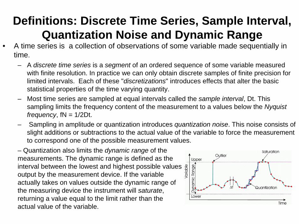
Definitions: Discrete Time Series, Sample Interval, Quantization Noise and Dynamic Range

• A time series is a collection of observations of some variable made sequentially in time.

– A discrete time series is a segment of an ordered sequence of some variable measured with finite resolution. In practice we can only obtain discrete samples of finite precision for limited intervals. Each of these "discretizations" introduces effects that alter the basic statistical properties of the time varying quantity.

– Most time series are sampled at equal intervals called the sample interval, Dt. This sampling limits the frequency content of the measurement to a values below the Nyquistfrequency, fN = 1/2Dt.

– Sampling in amplitude or quantization introduces quantization noise. This noise consists of slight additions or subtractions to the actual value of the variable to force the measurement to correspond one of the possible measurement values.

– Quantization also limits the dynamic range of the measurements. The dynamic range is defined as the interval between the lowest and highest possible values output by the measurement device. If the variable actually takes on values outside the dynamic range of the measuring device the instrument will saturate, returning a value equal to the limit rather than the actual value of the variable.

Definitions: Windowing, Fundamental Frequency, Extrema

– Selecting a finite segment of the time series is called windowing. It is as if the original time series is viewed through a window that only allows a finite segment to be seen.

– Often this window is a simple box-car, i.e. a function that is zero until the start of the segment, one during the segment, and zero after the segment. Windowing is accomplished by multiplying the original series by this window. This form of discretization also limits the frequency content of the data to frequencies higher than the fundamental frequency of the segment, f0 = 1/T, where T is the length of the sample.

– Assuming that the measurement is not saturated the time series will take on various values in the finite segment. One of these will be larger than all others, and one will be smaller. These extreme values for the time series are called the maximum and minimum.

– Simple programs often use these extremes to establish the scaling of time series plots. This scaling is usually a bad choice, particularly if the data contains a few outliers, or samples that are far from the typical values of the time series. Outliers are often produced by noise in the measurements, for example telemetry dropouts, lightening strikes, etc. When outliers are used to establish the extremes the plot consists mostly of white space with the data producing a nearly straight line and the noise producing the only variation.

Measures of Central Tendency: Mean, Median and Mode

• There are several common quantitative measures of the tendency for a variable to cluster around a central value including the mean, median, and mode.

–The mean of a set of Ntot observations of a discrete variable xi is defined as

–The median of a probability distribution function (pdf) p(x) is the value of xmedfor which larger and smaller values are equally probable. For discrete values, sort the samples xi into ascending order and if Ntot is odd find the value of xi that has equal numbers of points above and below it. If it is even this is not possible so instead take the average of the two central values of the sorted distribution.–The mode is defined as the value of xi corresponding to the maximum of the pdf. For a quantized variable like the Kp index this corresponds to the discrete value of Kp that occurs most frequently. More generally it is taken to be the value at the center of the bin containing the largest number of values. For continuous variables the definition depends on the width of bins used in determining the histogram. If the bins are too narrow there will be large fluctuations in the estimated pdf from bin to bin. If the bins are too large the location of the mode will be poorly resolved.

More on the Mode

• It is not necessary to create a histogram to obtain the mode of a distribution [Press et al., 1986, page 462]. It can be calculated directly from the data in the following manner.

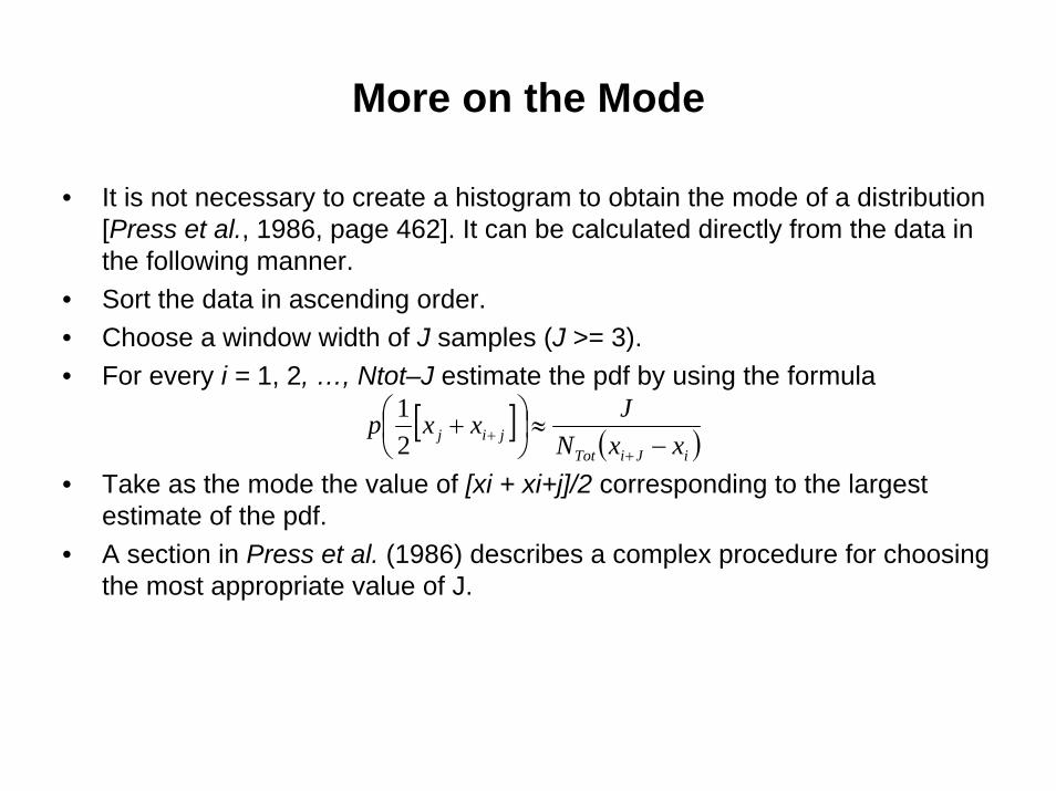
• Sort the data in ascending order. • Choose a window width of J samples (J >= 3). • For every i = 1, 2, …, Ntot–J estimate the pdf by using the formula

• Take as the mode the value of [xi + xi+j]/2 corresponding to the largest estimate of the pdf.

• A section in Press et al. (1986) describes a complex procedure for choosing the most appropriate value of J.

[ ] ( )iJiTotjij xxN

Jxxp−

≈⎟⎠⎞

⎜⎝⎛ +

++2

1

Kp and Dst

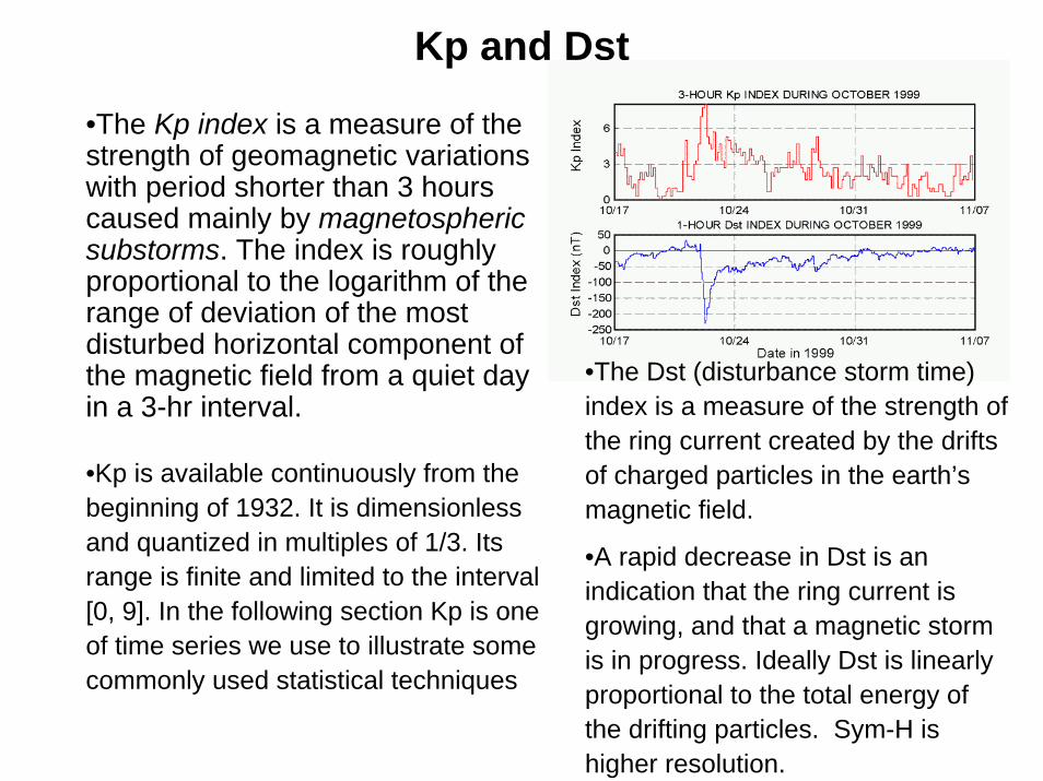
•The Kp index is a measure of the strength of geomagnetic variations with period shorter than 3 hours caused mainly by magnetospheric substorms. The index is roughly proportional to the logarithm of the range of deviation of the most disturbed horizontal component of the magnetic field from a quiet day in a 3-hr interval.

•Kp is available continuously from the beginning of 1932. It is dimensionless and quantized in multiples of 1/3. Its range is finite and limited to the interval [0, 9]. In the following section Kp is one of time series we use to illustrate some commonly used statistical techniques

•The Dst (disturbance storm time) index is a measure of the strength of the ring current created by the drifts of charged particles in the earth’s magnetic field.

•A rapid decrease in Dst is an indication that the ring current is growing, and that a magnetic storm is in progress. Ideally Dst is linearly proportional to the total energy of the drifting particles. Sym-H is higher resolution.

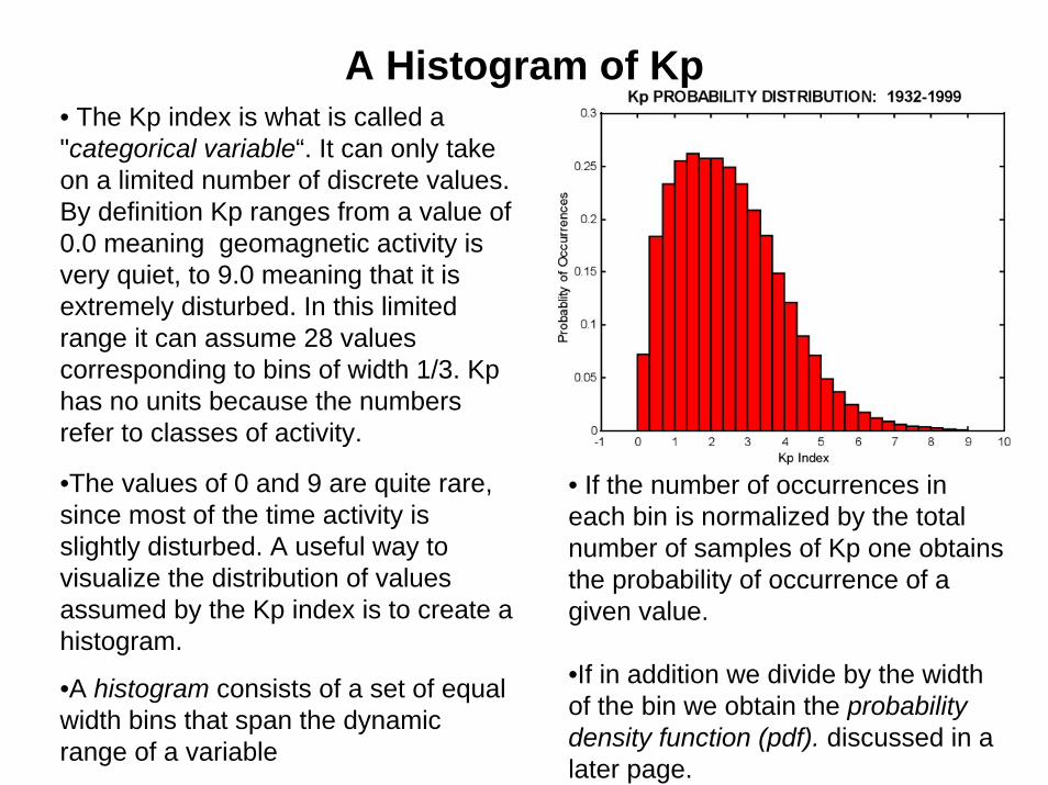
A Histogram of Kp• The Kp index is what is called a "categorical variable“. It can only take on a limited number of discrete values. By definition Kp ranges from a value of 0.0 meaning geomagnetic activity is very quiet, to 9.0 meaning that it is extremely disturbed. In this limited range it can assume 28 values corresponding to bins of width 1/3. Kphas no units because the numbers refer to classes of activity.

•The values of 0 and 9 are quite rare, since most of the time activity is slightly disturbed. A useful way to visualize the distribution of values assumed by the Kp index is to create a histogram.

•A histogram consists of a set of equal width bins that span the dynamic range of a variable

• If the number of occurrences in each bin is normalized by the total number of samples of Kp one obtains the probability of occurrence of a given value.

•If in addition we divide by the width of the bin we obtain the probability density function (pdf). discussed in a later page.

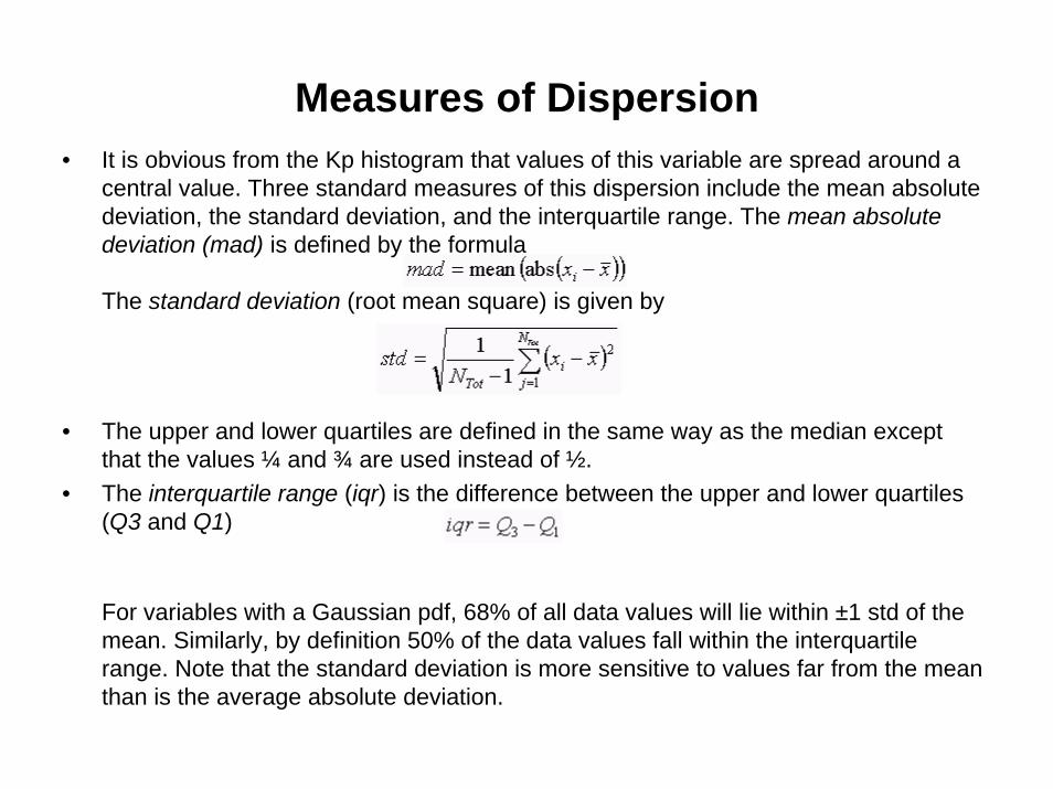
Measures of Dispersion• It is obvious from the Kp histogram that values of this variable are spread around a

central value. Three standard measures of this dispersion include the mean absolute deviation, the standard deviation, and the interquartile range. The mean absolute deviation (mad) is defined by the formula

The standard deviation (root mean square) is given by

• The upper and lower quartiles are defined in the same way as the median except that the values ¼ and ¾ are used instead of ½.

• The interquartile range (iqr) is the difference between the upper and lower quartiles (Q3 and Q1)

For variables with a Gaussian pdf, 68% of all data values will lie within ±1 std of the mean. Similarly, by definition 50% of the data values fall within the interquartilerange. Note that the standard deviation is more sensitive to values far from the mean than is the average absolute deviation.

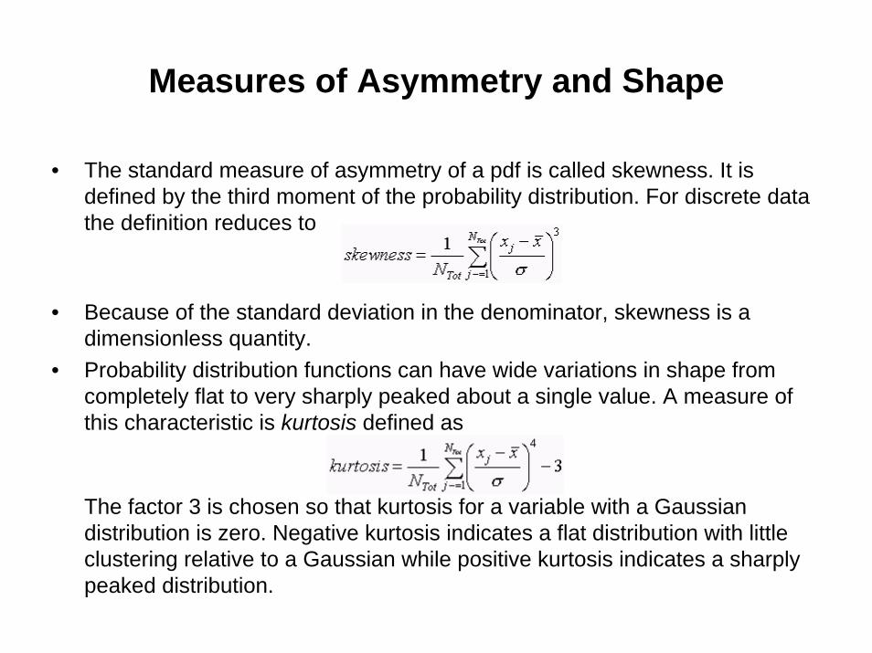
Measures of Asymmetry and Shape

• The standard measure of asymmetry of a pdf is called skewness. It is defined by the third moment of the probability distribution. For discrete data the definition reduces to

• Because of the standard deviation in the denominator, skewness is a dimensionless quantity.

• Probability distribution functions can have wide variations in shape from completely flat to very sharply peaked about a single value. A measure of this characteristic is kurtosis defined as

The factor 3 is chosen so that kurtosis for a variable with a Gaussian distribution is zero. Negative kurtosis indicates a flat distribution with little clustering relative to a Gaussian while positive kurtosis indicates a sharply peaked distribution.

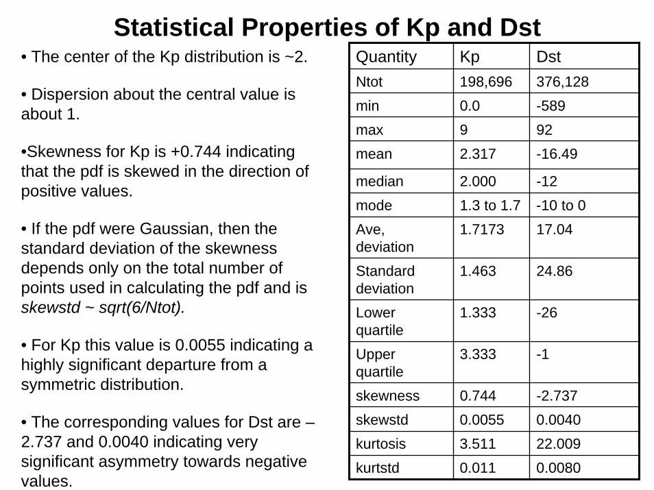
Statistical Properties of Kp and DstQuantity Kp DstNtot 198,696 376,128min 0.0 -589max 9 92mean 2.317 -16.49

median 2.000 -12mode 1.3 to 1.7 -10 to 0Ave, deviation

1.7173 17.04

Standard deviation

1.463 24.86

Lower quartile

1.333 -26

Upper quartile

3.333 -1

skewness 0.744 -2.737skewstd 0.0055 0.0040kurtosis 3.511 22.009kurtstd 0.011 0.0080

• The center of the Kp distribution is ~2.

• Dispersion about the central value is about 1.

•Skewness for Kp is +0.744 indicating that the pdf is skewed in the direction of positive values.

• If the pdf were Gaussian, then the standard deviation of the skewnessdepends only on the total number of points used in calculating the pdf and is skewstd ~ sqrt(6/Ntot).

• For Kp this value is 0.0055 indicating a highly significant departure from a symmetric distribution.

• The corresponding values for Dst are –2.737 and 0.0040 indicating very significant asymmetry towards negative values.

The Shape of the Kp and Dst Distributions

• Negative kurtosis indicates a flat distribution with little clustering relative to a Gaussian while positive kurtosis indicates a sharply peaked distribution.

– For Gaussian variables the standard deviation of the kurtosis also depends only on the total number of points used in calculating the pdf and is approximately kurtstd ~ sqrt(24/Ntot).

– Both distributions exhibit positive kurtosis, the Dst pdf to a greater extent than the Kp distribution. Thus the distributions for both indices are more sharply peaked than would be a Gaussian distribution.

The Probability Distribution Function 1

• Probability is the statistical concept that describes the likelihood of the occurrence of a specific event. It is estimated as the ratio of the number of ways the specific event might occur to the total number of all possible occurrences, i.e. P(x) = N(x)/Ntot. Suppose we have a random variable Xwith values lying on the x axis. The probability density p(x) for X is related to probability through an integral

• Suppose we have a sample set of Ntot observations of the variable X. The probability distribution function (pdf) for this variable at the point xi is defined as

• Here ∆x is the interval (or bin) of x over which occurrences of different values of X are accumulated, N[xi, xi+∆x] is the number of events found in the bin between xi and xi+∆x, and Ntot is the total number of samples in the set of observations of X.

The Probability Distribution Function 2

• Usually the sample set is not large enough to allow the limit to be achieved so that the pdf is approximated over a set of equal width bins defined by the bin edges {xi} = {x0, x0+∆x, x0+2∆x, x0+3∆x, …,, x0+m∆x}.

• Normally x0 and x0+m∆x are chosen so that all points in the sample set fall between these two limits.

• A plot of the quantity N[xi, xi+∆x] calculated for all values of x with a fixed ∆xis called a frequency histogram. The plot is called a probability histogramwhen the frequency of occurrence in each bin is normalized by the total number of occurrences, Ntot. The sum of all values of a probability histogram is 1.0.

• If the bin width is changed the occurrence probabilities will also change. To compensate for this the probability histogram is additionally normalized by the width of the bin to obtain the probability density function which we refer to as the probability distribution function. The sum of all values of the probability density distribution equals 1/∆x. The bin width ∆x is usually fixed, but in cases where some bins have very low occurrence probability it may be necessary to increase ∆x as a function of x.

The Probability Distribution Function 3

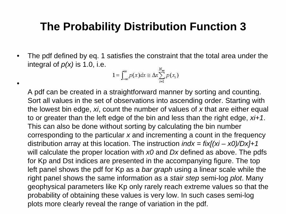
• The pdf defined by eq. 1 satisfies the constraint that the total area under the integral of p(x) is 1.0, i.e.

•A pdf can be created in a straightforward manner by sorting and counting. Sort all values in the set of observations into ascending order. Starting with the lowest bin edge, xi, count the number of values of x that are either equal to or greater than the left edge of the bin and less than the right edge, xi+1. This can also be done without sorting by calculating the bin number corresponding to the particular x and incrementing a count in the frequency distribution array at this location. The instruction indx = fix[(xi – x0)/Dx]+1 will calculate the proper location with x0 and Dx defined as above. The pdfsfor Kp and Dst indices are presented in the accompanying figure. The top left panel shows the pdf for Kp as a bar graph using a linear scale while the right panel shows the same information as a stair step semi-log plot. Many geophysical parameters like Kp only rarely reach extreme values so that the probability of obtaining these values is very low. In such cases semi-log plots more clearly reveal the range of variation in the pdf.

The Probability Distribution Function 4: Examples

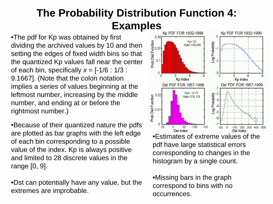
•The pdf for Kp was obtained by first dividing the archived values by 10 and then setting the edges of fixed width bins so that the quantized Kp values fall near the center of each bin, specifically x = [-1/6 : 1/3 : 9.1667]. (Note that the colon notation implies a series of values beginning at the leftmost number, increasing by the middle number, and ending at or before the rightmost number.)

•Because of their quantized nature the pdfsare plotted as bar graphs with the left edge of each bin corresponding to a possible value of the index. Kp is always positive and limited to 28 discrete values in the range [0, 9].

•Dst can potentially have any value, but the extremes are improbable.

•Estimates of extreme values of the pdf have large statistical errors corresponding to changes in the histogram by a single count.

•Missing bars in the graph correspond to bins with no occurrences.

Probability Distribution Functions: Kp and DstContinued

• Both Kp and Dst are not Gaussian, i.e. they do not have Gaussian shaped pdfs.

– By defintion Kp has finite range and is skewed to positive values. Its pdf values is peaked around Kp ~ 2. Both high and low values of Kp have a low probability of occurrence.

– The pdf for Dst is skewed to extreme negative values (note that the x-axis for Dsthas been reversed for comparison with the Kp distribution). Both large positive and negative values are rare. The most probable value of Dst is ~0. This property is a result of the definition of Dst that is designed to be approximately zero on the five quietest days of each month of the year.

Estimating PDFs: The Naïve Estimator• At the extremes of the distribution some bins will be empty while others

have only one or two occurrences. The calculated probability density will vary dramatically between adjacent bins due to fluctuations in the number of occurrences.

• Increasing the bin width does not help because this tends to filter out important details in portions of the distribution where there is sufficient data for narrow bins.

• The histogram can also hide important details of the distribution through the particular choice of the locations of the bin edges.

• The simplest form of PDF estimate is realized by sorting the sequence of observations into ascending order of and then centering bins on every sample in the sorted distribution. The pdf is then estimated at any x by

Num[] is the count of all values of Xi that fall in the bin of width 2h centered at x. To avoid infinities the point x is chosen at existing observations Xi. This technique guarantees that every estimate will be finite, containing one or more samples. It also eliminates the problem of where to place the bin edges.

Estimating PDFs: The Naïve Estimator Continued

• The counting procedure may be represented mathematically by a weighted sum as follows. Define a weight function w(x) by

• Then the estimate at a fixed point x is given by

• This formula is implemented by choosing a point x = Xi and then counting all observations that lie in the interval ±h of this location, then divide by the total number of observations Ntot to obtain the probability, and finally divide by the bin width 2h to obtain the probability density.

• To create a plot of the PDF of Dst a patch of width 2h = 10 nT and height corresponding to the log base 10 of the probability density was plotted about each unique value of Dst in the distribution.

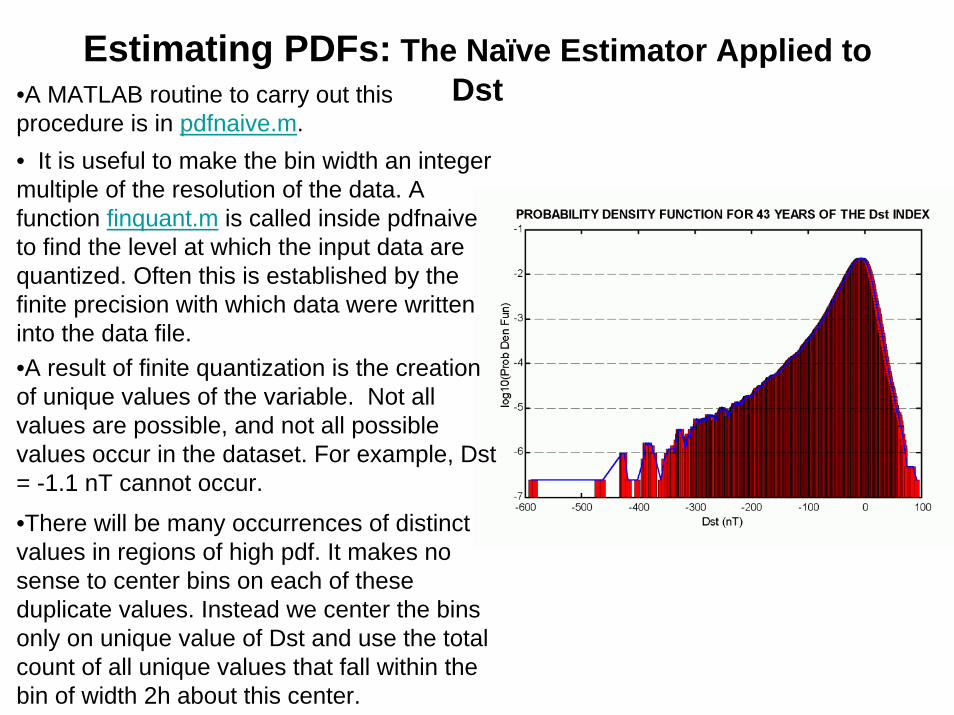
Estimating PDFs: The Naïve Estimator Applied to Dst•A MATLAB routine to carry out this

procedure is in pdfnaive.m.• It is useful to make the bin width an integer multiple of the resolution of the data. A function finquant.m is called inside pdfnaiveto find the level at which the input data are quantized. Often this is established by the finite precision with which data were written into the data file. •A result of finite quantization is the creation of unique values of the variable. Not all values are possible, and not all possible values occur in the dataset. For example, Dst= -1.1 nT cannot occur.

•There will be many occurrences of distinct values in regions of high pdf. It makes no sense to center bins on each of these duplicate values. Instead we center the bins only on unique value of Dst and use the total count of all unique values that fall within the bin of width 2h about this center.

Estimating PDFs: The Nearest Neighbor• The difficulty with the naive pdf estimator discussed on the previous page is

the requirement that all bins are the same width. • A better estimate could be obtained by requiring that the width of the bin be

inversely proportional to the density of observations around a point. This estimate is called the nearest neighbor pdf.

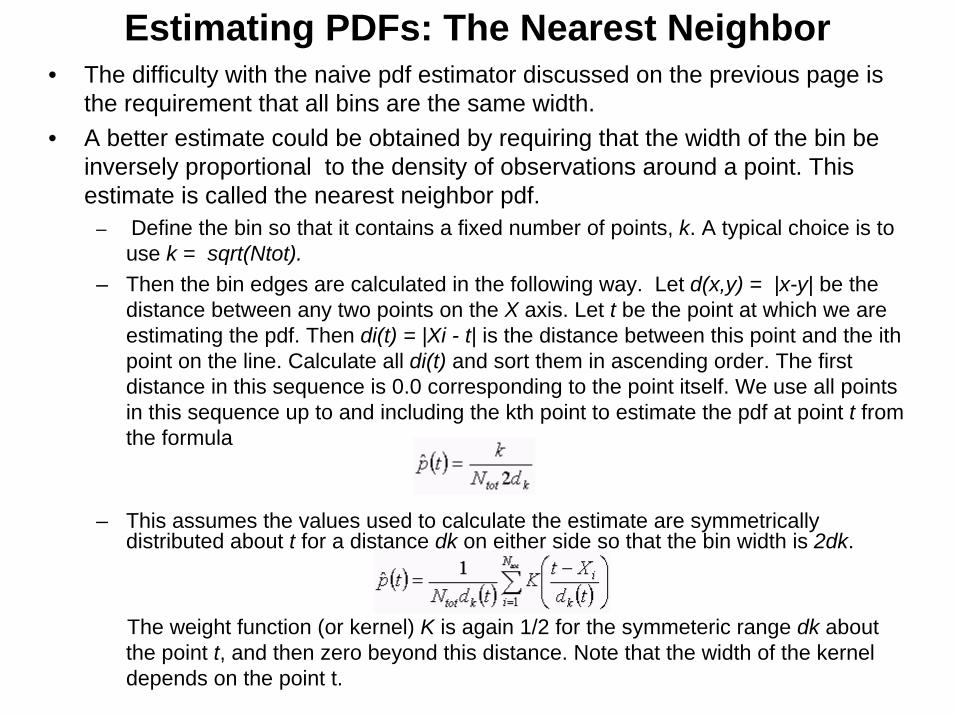
– Define the bin so that it contains a fixed number of points, k. A typical choice is to use k = sqrt(Ntot).

– Then the bin edges are calculated in the following way. Let d(x,y) = |x-y| be the distance between any two points on the X axis. Let t be the point at which we are estimating the pdf. Then di(t) = |Xi - t| is the distance between this point and the ithpoint on the line. Calculate all di(t) and sort them in ascending order. The first distance in this sequence is 0.0 corresponding to the point itself. We use all points in this sequence up to and including the kth point to estimate the pdf at point t from the formula

– This assumes the values used to calculate the estimate are symmetrically distributed about t for a distance dk on either side so that the bin width is 2dk.

The weight function (or kernel) K is again 1/2 for the symmeteric range dk about the point t, and then zero beyond this distance. Note that the width of the kernel depends on the point t.

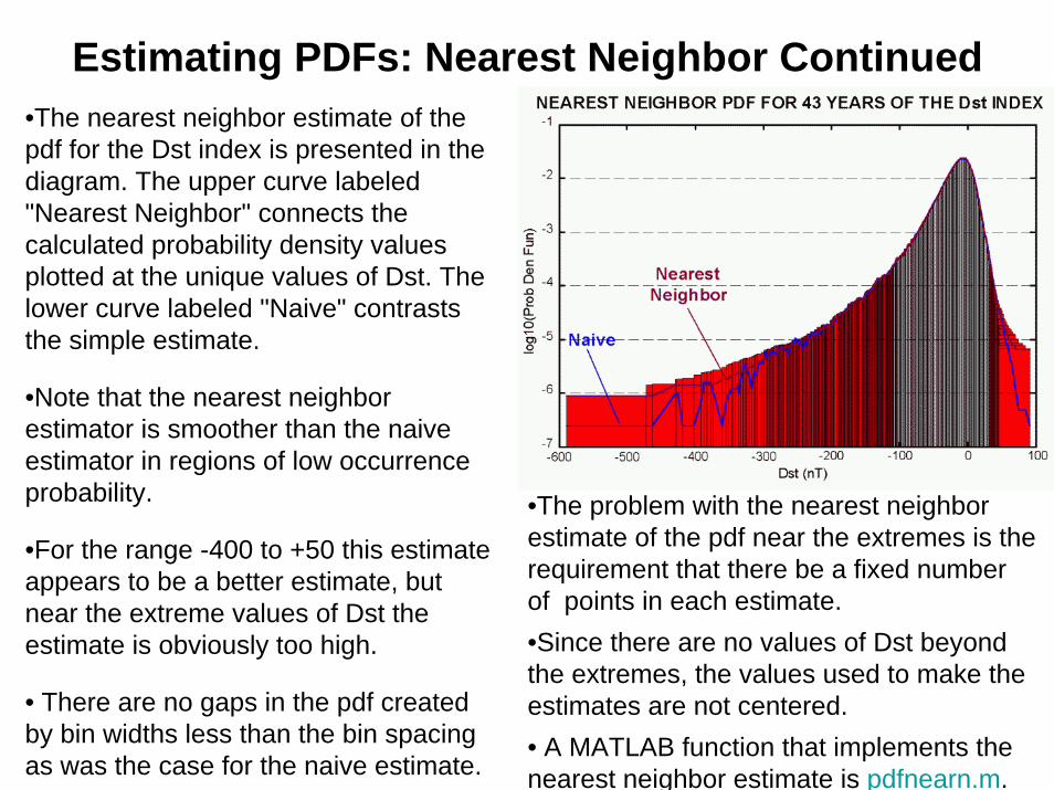
Estimating PDFs: Nearest Neighbor Continued•The nearest neighbor estimate of the pdf for the Dst index is presented in the diagram. The upper curve labeled "Nearest Neighbor" connects the calculated probability density values plotted at the unique values of Dst. The lower curve labeled "Naive" contrasts the simple estimate.

•Note that the nearest neighbor estimator is smoother than the naive estimator in regions of low occurrence probability.

•For the range -400 to +50 this estimate appears to be a better estimate, but near the extreme values of Dst the estimate is obviously too high.

• There are no gaps in the pdf created by bin widths less than the bin spacing as was the case for the naive estimate.

•The problem with the nearest neighbor estimate of the pdf near the extremes is the requirement that there be a fixed number of points in each estimate. •Since there are no values of Dst beyond the extremes, the values used to make the estimates are not centered.• A MATLAB function that implements the nearest neighbor estimate is pdfnearn.m.

Estimating PDFs: The Kernel Estimate

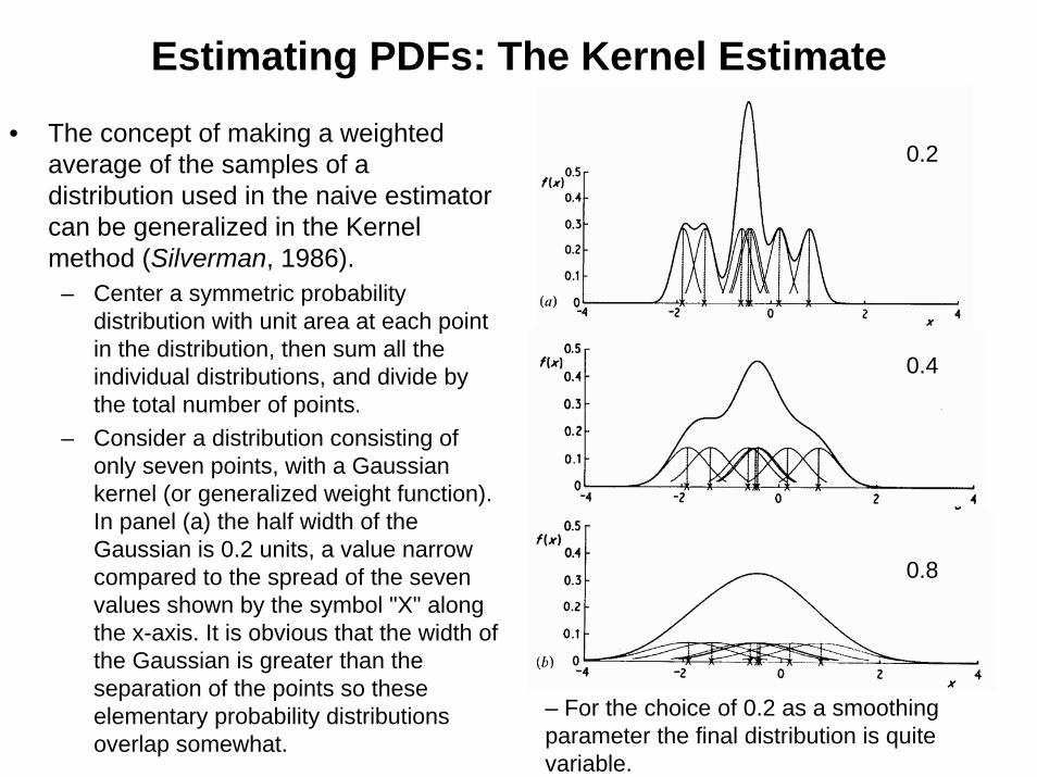
• The concept of making a weighted average of the samples of a distribution used in the naive estimator can be generalized in the Kernel method (Silverman, 1986).

– Center a symmetric probability distribution with unit area at each point in the distribution, then sum all the individual distributions, and divide by the total number of points.

– Consider a distribution consisting of only seven points, with a Gaussian kernel (or generalized weight function). In panel (a) the half width of the Gaussian is 0.2 units, a value narrow compared to the spread of the seven values shown by the symbol "X" along the x-axis. It is obvious that the width of the Gaussian is greater than the separation of the points so these elementary probability distributions overlap somewhat.

– For the choice of 0.2 as a smoothing parameter the final distribution is quite variable.

0.4

0.2

0.8

Estimating PDFs: The Kernel Estimate Continued

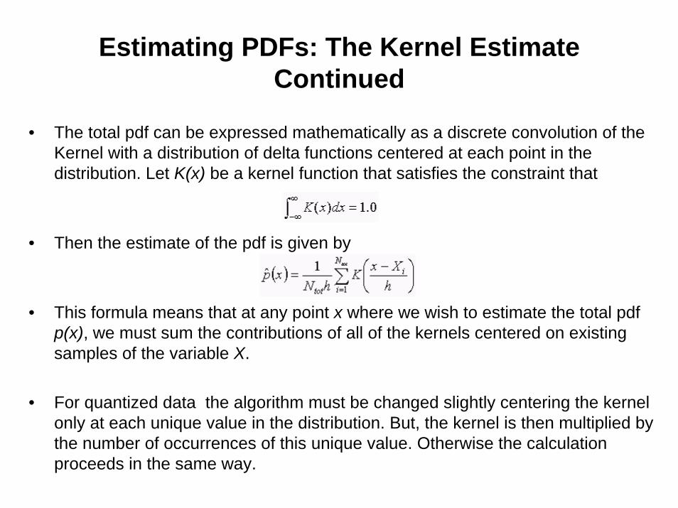
• The total pdf can be expressed mathematically as a discrete convolution of the Kernel with a distribution of delta functions centered at each point in the distribution. Let K(x) be a kernel function that satisfies the constraint that

• Then the estimate of the pdf is given by

• This formula means that at any point x where we wish to estimate the total pdfp(x), we must sum the contributions of all of the kernels centered on existing samples of the variable X.

• For quantized data the algorithm must be changed slightly centering the kernel only at each unique value in the distribution. But, the kernel is then multiplied by the number of occurrences of this unique value. Otherwise the calculation proceeds in the same way.

Estimating PDFs: The Kernel Method Continued

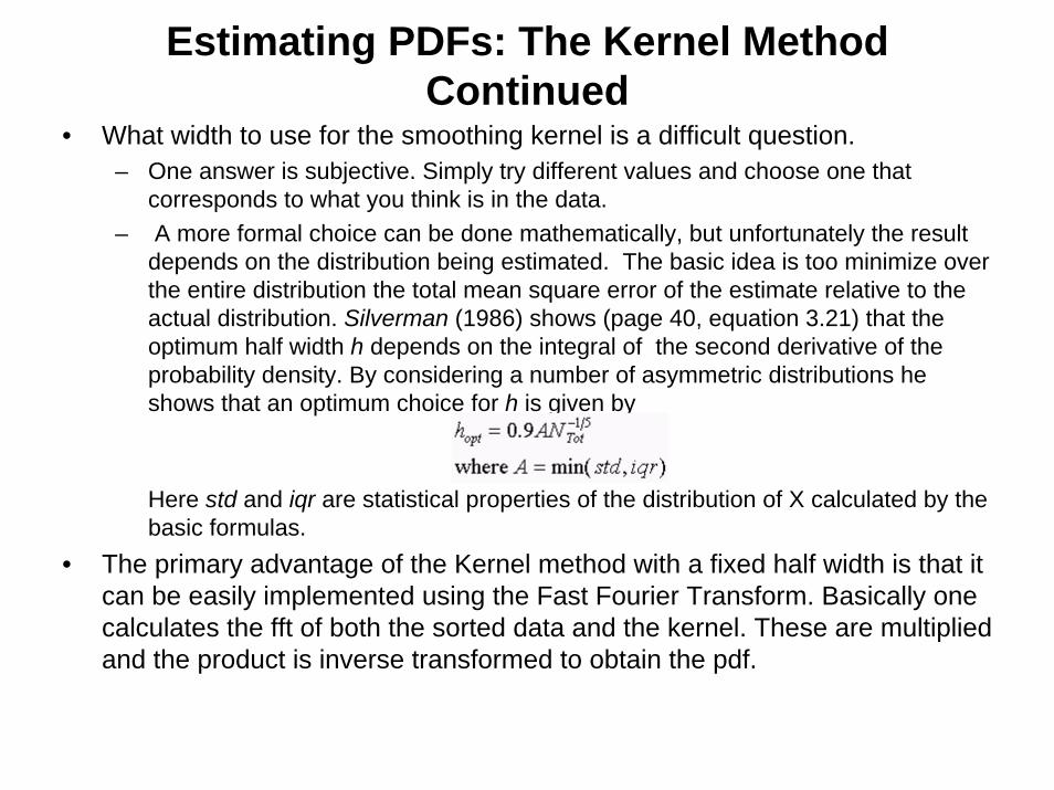
• What width to use for the smoothing kernel is a difficult question. – One answer is subjective. Simply try different values and choose one that

corresponds to what you think is in the data.– A more formal choice can be done mathematically, but unfortunately the result

depends on the distribution being estimated. The basic idea is too minimize over the entire distribution the total mean square error of the estimate relative to the actual distribution. Silverman (1986) shows (page 40, equation 3.21) that the optimum half width h depends on the integral of the second derivative of the probability density. By considering a number of asymmetric distributions he shows that an optimum choice for h is given by

Here std and iqr are statistical properties of the distribution of X calculated by the basic formulas.

• The primary advantage of the Kernel method with a fixed half width is that it can be easily implemented using the Fast Fourier Transform. Basically one calculates the fft of both the sorted data and the kernel. These are multiplied and the product is inverse transformed to obtain the pdf.

Estimating PDFs: The Kernel Method Continued

• One important detail in this approach is to avoid errors due to circular convolution (See Otnes and Enochson, 1978). These occur because the fftfunction assumes that the underlying data are periodic with period equal to the length of the data sample, i.e. the total number of points. These errors can be eliminated by the use of zero padding. One simply loads the data into arrays that are twice as long as the original data array. These arrays are then handled as described above. Circular convolution occurs, but since the last half of each array is zero, no information is passed from the right edge of the arrays to the left in the transform process. After multiplying the transforms and inverse transforming one gets the correct result for the convolution.

• We have implemented this procedure in a MATLAB function pdfkernel.m

Estimating PDFs: The Kernel Method Continued

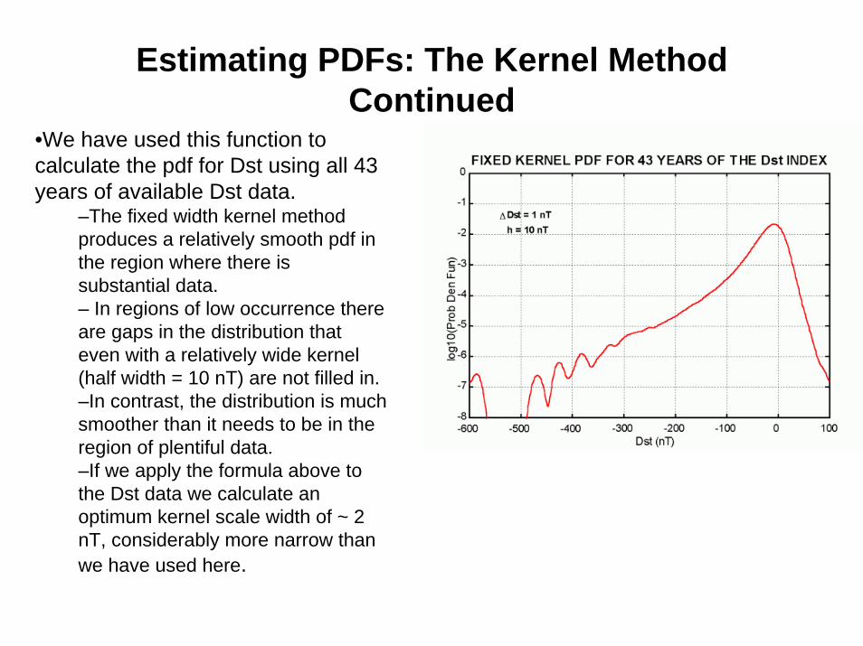
•We have used this function to calculate the pdf for Dst using all 43 years of available Dst data.

–The fixed width kernel method produces a relatively smooth pdf in the region where there is substantial data.– In regions of low occurrence there are gaps in the distribution that even with a relatively wide kernel (half width = 10 nT) are not filled in. –In contrast, the distribution is much smoother than it needs to be in the region of plentiful data. –If we apply the formula above to the Dst data we calculate an optimum kernel scale width of ~ 2 nT, considerably more narrow than we have used here.

Estimating the PDF: The Adaptive Kernel• The nearest neighbor estimate of the pdf suffers from the problem of

asymptotically approaching infinity so slowly that the total area of the calculated pdf is infinite. This problem arises from the absence of any pointsbeyond the extremes and therefore the use of values of the variable from regions of higher probability density to make the extreme estimates.

• The adaptive kernel:– Create a pilot pdf using the naive estimator – Create a pdf array on a grid of X spaced by Dx between the extremes of X and

initialize all values to 0.0. – Start with the lowest unique value of X and step sequentially through all unique

values – For each unique value Xi calculate the number of occurrences of the value,

N(Xi). – At each unique value Xi create a symmetric, non-negative, finite width Kernel

with area = 1.0, and a scale l inversely proportional to the probability density as determined in the pilot pdf.

– Evaluate the Kernel everywhere on the pdf grid– Multiply the Kernel by N(Xi) and add to the pdf array – Repeat for all unique values of the variable

Estimating the PDF- The Adaptive Kernel Continued

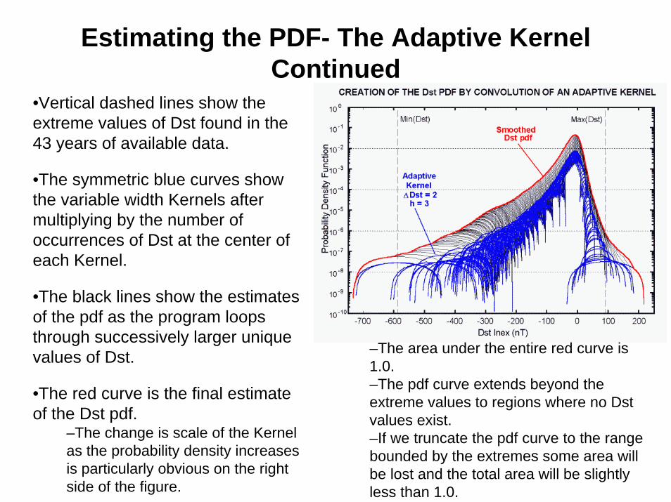
•Vertical dashed lines show the extreme values of Dst found in the 43 years of available data.

•The symmetric blue curves show the variable width Kernels after multiplying by the number of occurrences of Dst at the center of each Kernel.

•The black lines show the estimates of the pdf as the program loops through successively larger unique values of Dst.

•The red curve is the final estimate of the Dst pdf.

–The change is scale of the Kernel as the probability density increases is particularly obvious on the right side of the figure.

–The area under the entire red curve is 1.0. –The pdf curve extends beyond the extreme values to regions where no Dstvalues exist. –If we truncate the pdf curve to the range bounded by the extremes some area will be lost and the total area will be slightly less than 1.0.

Estimating the PDF: The Adaptive Kernel Continued

• A MATLAB function that implements the adaptive Kernel estimate of the pdfis pdfadap.m.

• The function pdfadap.m makes several assumptions as well as compromises.

– First, to avoid Kernels of infinite width (such as Gaussians) we used the Epanechnikov Kernel which is a parabola opening downward with finite normalized width of ±sqrt(5).

– We have fixed the parameter that controls the sensitivity of the Kernel scale to details of the pilot distribution to be a = 0.5 (See Silverman, 1996).

– We have set the local Kernel scale (lh) using the expression l = 1 + ( pilot/g)(-a). Note that the term "1 + " is not given in Silverman. I have added it to force the local bandwidth factors li to approach 1.0 rather than 0.0 as the pilot pdfbecomes large. If I don't do this the final kernel gets smaller than the basic smoothing factor h, and smaller than the spacing of the pdf and causes problems with data that has finite quantization. This effectively forces the Kernel to include at least three sample points on the pdf array.

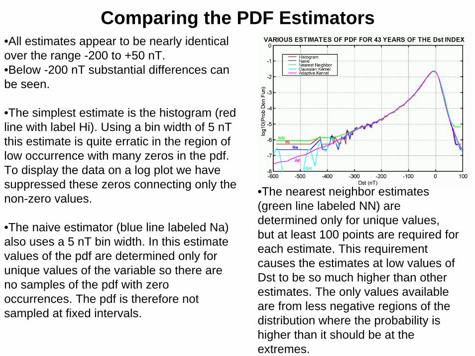
Comparing the PDF Estimators•All estimates appear to be nearly identical over the range -200 to +50 nT. •Below -200 nT substantial differences can be seen.

•The simplest estimate is the histogram (red line with label Hi). Using a bin width of 5 nTthis estimate is quite erratic in the region of low occurrence with many zeros in the pdf. To display the data on a log plot we have suppressed these zeros connecting only the non-zero values.

•The naive estimator (blue line labeled Na) also uses a 5 nT bin width. In this estimate values of the pdf are determined only for unique values of the variable so there are no samples of the pdf with zero occurrences. The pdf is therefore not sampled at fixed intervals.

•The nearest neighbor estimates (green line labeled NN) are determined only for unique values, but at least 100 points are required for each estimate. This requirement causes the estimates at low values of Dst to be so much higher than other estimates. The only values available are from less negative regions of the distribution where the probability is higher than it should be at the extremes.

Comparing the PDF Estimators Continued

• The fixed width Gaussian kernel estimate (cyan curve lebeled GK) was determined by sampling the pdf uniformly every 1 nT using a Gaussian kernel of half width 10 nT. This width is really too wide for the central part of the distribution and too narrow for the left edge. The absence of Dst values below -350 is emphasized by the Gaussian shaped humps centered on unique values of Dst.

• The adaptive Kernel (magenta curve labeled AK) estimate used an Epanechnikov kernel that is never smaller than three sample points on the final pdf (2 nT). At the extremes the bin width is much wider. This estimate is quite smooth everywhere and appears to approximate the scattered data at low values of Dst.