Introduction to Bayesian Estimation

June 1, 2012

The Plan

1. What is Bayesian statistics? How is it different fromfrequentist methods?

2. 4 Bayesian Principles

3. Priors: From prior information to prior distributions

The material in today’s lecture can be found in any good textbook on Bayesian statistics. One good example is Christian P.Robert’s The Bayesian Choice: From decision theoretic foundationsto Computational Implementation

Probability and statistics; What’s the difference?

Probability is a branch of mathematics

I There is little disagreement about whether the theoremsfollow from the axioms

Statistics is an inversion problem: What is a good probabilisticdescription of the world, given the observed outcomes?

I There is some disagreement about how we interpretdata/observations

Why probabilistic models?

Is the world characterized by randomness?

I Is the weather random?

I Is a coin flip random?

I ECB interest rates?

What is the meaning of probability, randomness anduncertainty?

Two main schools of thought:

I The classical (or frequentist) view is that probabilitycorresponds to the frequency of occurrence in repeatedexperiments

I The Bayesian view is that probabilities are statements aboutour state of knowledge, i.e. a subjective view.

The difference has implications for how we interpret estimatedstatistical models and there is no general agreement about whichapproach is “better”.

Frequentist vs Bayesian statistics

Variance of estimator vs variance of parameter

I Bayesians think of parameters as having distributions whilefrequentist conduct inference by thinking about the varianceof an estimator

Frequentist confidence intervals:

I If point estimates are the truth and with repeated draws fromthe population of equal sample length, what is the intervalthat θ̂ lies in 95 per cent of the time?

Bayesian probability intervals:

I Conditional on the observed data, a prior distribution of θ anda functional form (i.e. model), what is the shortest intervalthat with 95% contains θ?

The main conceptual difference is that Bayesians condition on thedata while frequentist design procedures that work well ex ante.

Frequentist vs Bayesian statistics

Coin flip example:

After flipping a coin 10 times and counting the number of heads,what is the probability that the next flip will come up heads?

I A Bayesian with a uniform prior would say that the probabilityof the next flip coming up heads is x/10 and where x is thenumber of times the flip came up heads in the observedsample

I A frequentist cannot answer this question: A frequentistconfidence interval can only be used to compute theprobability of having observed the sample conditional on agiven null hypothesis about the probability of heads vs tails.

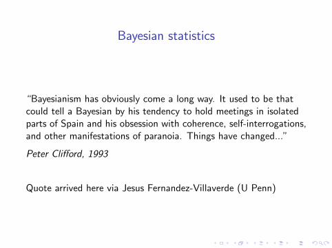
Bayesian statistics

“Bayesianism has obviously come a long way. It used to be thatcould tell a Bayesian by his tendency to hold meetings in isolatedparts of Spain and his obsession with coherence, self-interrogations,and other manifestations of paranoia. Things have changed...”

Peter Clifford, 1993

Quote arrived here via Jesus Fernandez-Villaverde (U Penn)

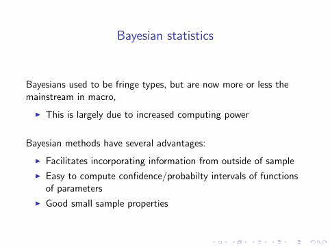
Bayesian statistics

Bayesians used to be fringe types, but are now more or less themainstream in macro,

I This is largely due to increased computing power

Bayesian methods have several advantages:

I Facilitates incorporating information from outside of sample

I Easy to compute confidence/probabilty intervals of functionsof parameters

I Good small sample properties

The subjective view of probability

What does subjective mean?

I Coin flip: What is prob(heads) after flip but before looking?

Important: Probabilities can be viewed as statements about ourknowledge of a parameter, even if the parameter is a constant

I E.g. treating risk aversion as a random variable does notimply that we think of it as varying across time.

The subjective view of probability

Is a subjective view of probability useful?

I Yes, it allow people to incorporate information from outsidethe sample

I Yes, because subjectivity is always there (it just more hiddenin frequentist methods)

I Yes, because one can use “objective”, or non-informativepriors

I And: Sensitivity to priors can be checked

4 Principle of Bayesian Statistics

1. The Likelihood Principle

2. The Sufficiency Principle

3. The Conditionality Principle

4. The Stopping Rule Principle

These are principles that appeal to “common sense”.

The Likelihood Principle

All the information about a parameter from an experiment iscontained in the likelihood function

The Likelihood Principle

The likelihood principle can be derived from two other principles:

I The Sufficiency Principle

I If two samples imply the same sufficient statistic (given amodel that admits such a thing), then they should lead to thesame inference about θ

I Example: Two samples from a normal distribution with thesame mean and variance should lead to the same inferenceabout the parameters µ and σ2

I The Conditionality Principle

I If there are two possible experiments on the parameter θ isavailable, and one of the experiments is chosen withprobability p then the inference on θ should only depend onthe chosen experiment

The Stopping Rule Principle

The Stopping Rule Principle is an implication of the LikelihoodPrinciple

If a sequence of experiments, ε1, ε2, ..., is directed by a stoppingrule, τ , which indicates when the experiment should stop, inferenceabout θ should depend on τ only through the resulting sample.

The Stopping Rule Principle: Example

In an experiment to find out the fraction of the population thatwatched a TV show, a researcher found 9 viewers and and 3non-viewers.

Two possible models:

1. The researcher interviewed 12 people and thus observedx ∼ B(12, θ)

2. The researcher questions N people until he obtained 3non-viewers with N ∼ Neg(3, 1− θ)

The likelihood principle implies that the inference about θ shouldbe identical if either model was used. A frequentist would drawdifferent conclusions depending on wether he thought (1) or (2)generated the experiment.In fact, H0 : θ > 0.5 would be rejected if experiment is (2) but notif it is (1).

The Stopping Rule Principle

“...a hypothesis which may be true may be rejected because it hasnot predicted observable results which have not occurred.”Jeffreys (1961)

“I learned the stopping rule principle from Professor Barnard, inconversation in the summer of 1952. Frankly, I thought it ascandal that anyone in the profession could advance an idea sopatently wrong, even as today I can scarcely believe that somepeople resist an idea so patently right”Savage (1962)

Quotes (again) arrived here via Jesus Fernandez-Villaverde (UPenn)

Main concepts and notation

The main components in Bayesian inference are:

I Data (observables) ZT ∈ RT×n

I A model:

I Parameters θ ∈ Rk

I A prior distribution p(θ) : Rk −→ R+

I Likelihood function p(Z | θ) : RT×n × Rk −→ R+

The end product of Bayesian statistics

Most of Bayesian econometrics consists of simulating distributionsof parameters using numerical methods.

I A simulated posterior is a numerical approximation to thedistribution p(Z | θ)p(θ)

I This is useful since the the distribution p(Z | θ)p(θ) (byBayes’ rule) is proportional to p(θ | Z )

I We rely on ergodicity, i.e. that the moments of theconstructed sample correspond to the moments of thedistribution p(θ | Z )

The most popular procedure to simulate the posterior is called theRandom Walk Metropolis Algorithm

The MCMC with J=1000

0 100 200 300 400 500 600 700 800 900 10000.82

0.84

0.86

0.88

0.9

0.92

0.94

0.96

0 100 200 300 400 500 600 700 800 900 10002

4

6

8

10

12

14x 10

-3

The Histograms of MCMC with J=1000

0.82 0.84 0.86 0.88 0.9 0.92 0.94 0.960

10

20

30

40

50

60

70

80

90

100

2 4 6 8 10 12 14

x 10-3

0

20

40

60

80

100

120

The MCMC with J=1000 000

0 100 200 300 400 500 600 700 800 900 10000.7

0.75

0.8

0.85

0.9

0.95

1

0 100 200 300 400 500 600 700 800 900 10000.007

0.008

0.009

0.01

0.011

0.012

0.013

0.014

The Histograms of MCMC with J=1000 000

0.7 0.75 0.8 0.85 0.9 0.95 10

10

20

30

40

50

60

0.007 0.008 0.009 0.01 0.011 0.012 0.013 0.0140

10

20

30

40

50

60

70

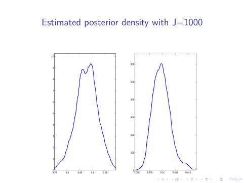
Estimated posterior density with J=1000

0.75 0.8 0.85 0.9 0.950

1

2

3

4

5

6

7

8

9

10

0.008 0.009 0.01 0.011 0.0120

100

200

300

400

500

600

Choosing priors

How influential the priors will be for the posterior is a choice:

I It is always possible to choose priors such that a given result isachieved no matter what the sample information is (i.e.dogmatic priors)

I It is also possible to choose priors such that they do notinfluence the posterior (i.e. so-called non-informative priors)

Important: Priors are a choice and must be motivated.

Combining prior and sample information

Sometimes we know more about the parameters than what thedata tells us, i.e. we have some prior information.

I For a DSGE model, we may have information about ”deep”parameters

I Range of some parameters may be restricted by theory, e.g.risk aversion should be positive

I Discount rate is inverse of average real interest ratesI Price stickiness can be measured by surveys

I We may know something about the mean of a process

How do we combine prior and sample information?

Bayes’ theorem:

P (θ | Z ) P(Z ) = P (Z | θ) P(θ)

⇔

P (θ | Z ) =P (Z | θ) P(θ)

P(Z )

I Since P(Z ) is constant (conditional on a particular model),we can use P (Z | θ) P(θ) as the posterior likelihood (alikelihood function is any function that is proportional to theprobability).

We now need to choose P(θ)

Choosing prior distributions

The beta distribution is a good choice when parameter is in [0,1]

P(x) =(1− x)b−1 xa−1

B(a, b)

where

B(a, b) =(a− 1)!(b − 1)!

(a + b − 1)!

Easier to parameterize using expression for mean, mode andvariance:

µ =a

a + b, x̂ =

a− 1

a + b − 2

σ2 =ab

(a + b)2 (a + b + 1)

Examples of beta distributions holding mean fixed

0 0.1 0.2 0.3 0.4 0.5 0.6 0.7 0.8 0.9 10

1

2

3

4

5

6

7

8

Examples of beta distributions holding s.d. fixed

0 0.1 0.2 0.3 0.4 0.5 0.6 0.7 0.8 0.9 10

2

4

6

8

10

12

14

16

18

Choosing prior distributions

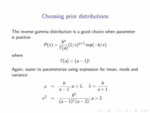
The inverse gamma distribution is a good choice when parameteris positive

P(x) =ba

Γ(a)(1/x)a+1 exp(−b/x)

whereΓ(a) = (a− 1)!

Again, easier to parameterize using expression for mean, mode andvariance:

µ =b

a− 1; a > 1, x̂ =

b

a + 1

σ2 =b2

(a− 1)2 (a− 2); a > 2

Examples of inverse gamma distributions

0 1 2 3 4 5 6 7 8 9 100

0.1

0.2

0.3

0.4

0.5

0.6

0.7

Conjugate Priors

Conjugate priors are a particularly convenient:

I Combining distributions that are members of a conjugatefamily result in a new distribution that is a member of thesame family

Useful, but only so far as that the priors are chosen to actuallyreflect prior beliefs rather than just for analytical convenience

Conjugate Priors: Examples

p(x |θ) p(θ) p(θ|x)

N(θ, σ2) N(µ, τ2) N((σ2 + τ2

)−1 (σ2µ+ τ2x

),(σ2 + τ2

)−1σ2τ2)

P(θ) G (α, β) G (α + x , β + 1)G (ν, θ) G (α, β) G (α + ν, β + x)

Improper Priors

Improper priors are priors that are not probability density functionsin the sense that they do not integrate to 1.

I Can still be used as a form of uninformative priors for sometypes of analysis

I The uniform distribution U(−∞,∞) is popular

I Mode of posterior then coincide with MLE.

Summing up

I It is important to understand what the subjective view ofprobability does and does not imply

I The Bayesian Principles

I Bayesians condition on the data

I Priors are chosen by the researcher and must be motivated

That’s it for today.