Embed Size (px)
Citation preview

- 1 -
Disentangling Classical and Bayesian Approaches to Uncertainty Analysis
Robin Willink1 and Rod White
2
1email: [email protected]
2Measurement Standards Laboratory
PO Box 31310, Lower Hutt 5040
New Zealand
email(corresponding author): [email protected]
Abstract Since the 1980s, we have seen a gradual shift in the uncertainty analyses recommended in the
metrological literature, principally Metrologia, and in the BIPM’s guidance documents; the Guide to
the Expression of Uncertainty in Measurement (GUM) and its two supplements. The shift has seen the
BIPM’s recommendations change from a purely classical or frequentist analysis to a purely Bayesian
analysis. Despite this drift, most metrologists continue to use the predominantly frequentist approach
of the GUM and wonder what the differences are, why there are such bitter disputes about the two
approaches, and should I change? The primary purpose of this note is to inform metrologists of the
differences between the frequentist and Bayesian approaches and the consequences of those
differences.
It is often claimed that a Bayesian approach is philosophically consistent and is able to tackle
problems beyond the reach of classical statistics. However, while the philosophical consistency of the
of Bayesian analyses may be more aesthetically pleasing, the value to science of any statistical analysis
is in the long-term success rates and on this point, classical methods perform well and Bayesian
analyses can perform poorly. Thus an important secondary purpose of this note is to highlight some of
the weaknesses of the Bayesian approach. We argue that moving away from well-established, easily-
taught frequentist methods that perform well, to computationally expensive and numerically inferior
Bayesian analyses recommended by the GUM supplements is ill-advised. Further, we recommend that
whatever methods are adopted, the metrology community should insist on proven long-term numerical
performance.
1. Introduction
Since 1993, uncertainty analysis in metrology has been practised in accordance with the Guide to the
Expression of Uncertainty in Measurement (GUM), which was originally published by the ISO (ISO
1993, 1995) but is now managed and published by the BIPM (JCGM 2008a). The GUM has led a
revolution in uncertainty analysis in metrology with increased emphasis now being placed on the
specification of a measurement model and increased attention being paid to quantifying influence
variables and sources of uncertainty. There seems to be little doubt that the greater attention given to
these aspects of measurement has come about from the single approach and the common language for
uncertainty analysis provided by the GUM.
For the most part, the GUM is fundamentally frequentist: the Type A assessment process, the
combination of uncertainties using the Welch-Satterthwaite formula, and the expression of expanded
uncertainties as confidence intervals are all demonstrably frequentist in origin and rationale. However,
the Type B assessment process, with its allusion to the concepts of degrees of belief and distributed
measurands, betrays a Bayesian thought process that is inconsistent with the philosophy of the
remainder of the guide. There are also aspects of uncertainty analysis that are not treated well or at all.
For example, the GUM fails to give satisfactory guidance on the handling of non-linearities,
corrections of just resolvable (non-significant) systematic effects, products of errors distributed about
zero, asymmetric error distributions, and multidimensional outputs such as for complex quantities.
Thus, the GUM can be viewed as a successful but imperfect set of guidelines.
In recent years, some of the technical deficiencies in the GUM have been addressed by
alternative methods, often supported by Monte Carlo analysis of the success rates of the method (e.g.,
Hall 2008, 2009, 2011, Wang and Iyer 2006, 2009). There has also been an increasing interest in
Bayesian statistics, which also uses Monte Carlo techniques, but for numerical integration rather than
evaluation of performance. The Bayesian approach is claimed by its practitioners to be more complete,
more universally applicable, and more philosophically consistent than the classical approach. Most
- 2 -
importantly, the Bayesian approach requires a formal assessment of the prior knowledge of the
measurand, which addresses concerns about the philosophy underlying the Type B assessment process
of the GUM.
Within Bayesian statistics there are two main divisions or schools, sometimes described as
‘subjective’ and ‘objective’. The principal criticism of subjective Bayesian statistics, as the name
suggests, is the highly personal nature of the probabilities that are used to describe prior knowledge.
The approach taken by the objective Bayesian school is to use ‘uninformative priors’ for their analyses
(JCGM 2008b, 2011). As we shall see, the Type A methodology of the GUM Supplements is largely
drawn from this objective school while the Type B methodology is drawn from the subjective Bayesian
school. The GUM supplements are therefore fundamentally Bayesian documents and philosophically
inconsistent with the GUM.
The change in recommended practice from classical (or frequentist) statistics to Bayesian
statistics seems to have been occurring with little input from metrologists; those who actually use
uncertainty analysis. Further, there is a degree to which history seems to be rewritten, with some
authors claiming that the fundamental approach taken in GUM is one of describing measurands by
distributions, as in a Bayesian analysis (e.g., Kacker et al 2007, Bich et al 2006). This paper
summarises the concerns we have about these developments. Some of the concerns relate to a change
in philosophy, which implies changes in measurement practice and in how scientists represent the
world. Other concerns are more practical: how do these changes impact the practical utility of
uncertainty analysis, and are they improving the situation? We suggest that these changes are most
definitely not trivial and we should be aware of their consequences. These issues have recently
increased in importance because of the announcement of plans to revise the GUM and the intention that
this revision will be along Bayesian lines (Bich et al 2006, Bich 2008, JCGM 2012)
Section 2 of this article discusses the rationale for uncertainty analysis. Section 3 is tutorial and
describes the basic differences between the frequentist and Bayesian approaches. It also briefly
describes the ‘fiducial’ view of data analysis, which is a view that some metrologists might hold
without realising it. Section 4 discusses how these different approaches appear in the BIPM documents
leading up to, including, and following on from the GUM of 1993/1995. Section 5 outlines various
implications of accepting a Bayesian approach to uncertainty analysis, as advocated in Supplements 1
and 2 to the GUM. Section 6 summarises and draws conclusions.
2. The rationale for uncertainty analysis
One of the characteristics of the debates between Bayesian and classical statisticians is a tendency to
talk past each other. The philosophies are so different that it seems impossible to find enough common
ground and understanding to enable a proper debate to occur. It is appropriate, therefore, that we set the
scene for the present debate about uncertainty analysis.
The rationale for uncertainty analysis does not seem to be well known or well understood by
many users of the analysis, even some metrologists. Certainly the school-days explanation that
“uncertainty is important because it measures the quality of the measurement”, is not especially helpful
as it provides no guidance of what uncertainty means in practice or how to evaluate it. Like many
measurement practices, clarity can often be found by looking at how uncertainties are used.
Consider a biscuit manufacturer who states on the packets that the net weight of biscuits in the
packets is 200 g. In New Zealand and many other countries, the practical meaning of such a statement
is tied to consumer protection regulations and to the Average Quantity System (AQS), which requires
the manufacturer to ensure that no packet is grossly under-filled and that the frequency of minor under-
fills is below some prescribed percentage. Ideally, the manufacturer understands that his measurements
of gross and net weight are subject to error processes that lead to both variability and bias. To be sure
of compliance with the AQS and to be confident that, say, 95% of the packets exceed the required net
weight, the accept-reject criterion imposed on product leaving the production line is increased above
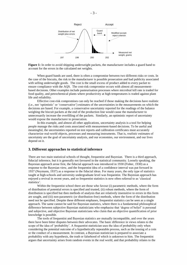
200 g to account for the measurement errors. This situation is shown graphically in Figure 1 where we
have characterised the measurement errors by a zero-mean (for simplicity) normal distribution. The
shaded area represents the probability that a packet with a true net weight of 199 g would be measured
to have a net weight exceeding 200 g and be accepted for sale. The addition of the guard band reduces
the chance of accepting this underweight packet.
- 3 -
Distribution of net
weight plus errors
200 198197 202
Reject Accept
Guard
band
Measured net
weight, grams
Modified accept-
reject criterion
Figure 1: In order to avoid shipping underweight packets, the manufacturer includes a guard band to
account for the errors in the calculated net weights.
When guard bands are used, there is often a compromise between two different risks or costs. In
the case of the biscuits, the risk to the manufacturer is possible prosecution and bad publicity associated
with selling underweight goods. The cost is the small excess of product added to every packet to
ensure compliance with the AQS. The cost-risk compromise occurs with almost all measurement-
based decisions. Other examples include pasteurisation processes where microbial kill rate is traded for
food quality, and petrochemical plants where productivity at high temperatures is traded against plant
life and reliability.
Effective cost-risk compromises can only be reached if those making the decisions have realistic
(i.e., not ‘optimistic’ or ‘conservative’) estimates of the uncertainties in the measurements on which the
decisions are based. For example, a conservative uncertainty reported for the readings of the balance
weighing the biscuit packets at the end of the production line would cause the manufacturer to
unnecessarily increase the overfilling of the packets. Similarly, an optimistic report of uncertainty
would expose the manufacturer to prosecution.
In this example, and almost all other applications, uncertainty analysis is a tool for helping
people manage the risks and costs associated with measurement-based decisions. To be useful and
meaningful, the uncertainties reported on test reports and calibration certificates must accurately
characterize real-world objects, processes and measuring instruments. That is, realistic estimates of
uncertainty are the goal of uncertainty analysis, and our economies, our environment, and our lives
depend on it.
3. Different approaches to statistical inference
There are two main statistical schools of thought, frequentist and Bayesian. There is a third approach,
fiducial inference, but it is generally not favoured in the statistical community. Loosely speaking, the
Bayesian approach arose first, the fiducial approach was introduced in 1930 (Fisher, 1930) as a
response to the Bayesian view, and the frequentist idea of a confidence interval was put forward in
1937 (Neymann, 1937) as a response to the fiducial ideas. For many years, the only type of statistics
taught at high-schools and university undergraduate level was frequentist. The Bayesian approach has
enjoyed a revival in recent years, and so frequentist statistics is now often referred to as ‘classical
statistics’.
Within the frequentist school there are those who favour (i) parametric methods, where the form
of distribution of potential errors is specified and trusted, (ii) robust methods, where the form of
distribution is specified but then methods of analysis that are relatively insensitive to errors in this form
are sought, and (iii) non-parametric (or distribution-free) methods, where the form of the distribution
need not be specified. Despite these different emphases, frequentist statistics can be seen as a single
approach. The same cannot be said for Bayesian statistics, where there is a fundamental philosophical
difference between subjective Bayesian statisticians who emphasise that ‘degree of belief’ is personal
and subjective, and objective Bayesian statisticians who claim that an objective quantification of prior
knowledge is possible.
The tools of frequentist and Bayesian statistics are mutually incompatible, and over the years
there have been bitter disputes between their advocates. The basic difference in views relates to the
scope of the idea of ‘probability’. A frequentist statistician uses the idea of probability only when
considering the potential outcome of a hypothetically repeatable process, such as the tossing of a coin
or the conduct of a measurement. In contrast, a Bayesian statistician is prepared to associate a
probability with any hypothesis, the truth or falsehood of which is unknown to him. The frequentist
argues that uncertainty arises from random events in the real world, and that probability relates to the
- 4 -
observed frequency of those events. The Bayesian argues that uncertainty arises because of the
observer’s lack of knowledge about the world, and, therefore, uncertainty lies within the observer’s
mind and probability measures a degree of belief.
To further elaborate on the differences, consider the idea that Barack Obama will be re-elected
in the forthcoming US presidential election. A frequentist would be unwilling to attribute any
numerical probability to this event because the election cannot be seen as a hypothetically repeatable
process. However, a Bayesian statistician would consider it legitimate to attribute a probability to
represent his strength of belief about the outcome. In the same way, a Bayesian would have no qualms
attributing a probability to the hypothesis that Boltzmann’s constant, k, exceeds 1.38065 10
J K
,
but a frequentist would find no meaning in this idea. The relationship attributed a probability,
k > 1.38065 10
J K
, is a relationship between two constants, one an unknown fundamental
constant of nature, and the other an explicit real number. No hypothetically repeatable experiment can
be envisaged when such a statement is made, so this is not a usage of probability that a frequentist
would regard as scientific. (Note that colloquial usage of the term probability is often consistent with
the Bayesian interpretation.)
The idea that probability means ‘degree of belief’ to a Bayesian but not to a frequentist is often
said to be the difference between the two approaches. However, this distinction is not especially helpful
or discerning. The probability a frequentist attributes to an event clearly describes his degree of belief
about the next outcome of a repeatable process, so a frequentist probability is also interpretable as a
degree of belief. Thus, focusing on the nature of probability misses the point; instead the difference is
found in the scope of probability. Frequentists only attribute probabilities in situations where
probability assignments are potentially testable by repetition. Bayesians do not require repeatability and
testability.
3.1 Frequentist statistics and confidence intervals
For the frequentist, a numerical value of a probability is the limit of relative frequency in a large
number of trials. In the scientific context, an experiment is considered to be one of an infinite sequence
of possible repetitions of the same experiment. The experiment is understood to involve the drawing of
observations (samples) from a distribution representing the population of potential observations. Before
the sampling, a technique of analysis will have been found that, with respect to the randomness in this
sampling, has a specified high probability of leading to a correct conclusion being drawn.
The basic tool of the frequentist statistician is the ‘confidence interval’, which is a random
interval with a specified probability of covering the parameter being estimated. For example, if we
employ a 95% confidence interval for the unknown mean of a population then there is a probability of
0.95 that the sampling process will result in a statement “lower limit unknown mean upper limit”
that is true.
Example 1: Frequentist measurement of Boltzmann’s constant
Suppose we wish to measure Boltzmann’s constant, k, using an unbiased method that is known to
generate normally distributed errors. So k is the unknown mean of the potential population of
measurement results, and the task of the measurement is to estimate this mean.
The first step is to define the statistical model of the process and the analysis procedure. In this
case, we will make n individual measurements of k and we assume that the n observations will be
drawn independently from a normal (Gaussian) distribution with unknown mean k and unknown
standard deviation We let X denote the random variable for the sample mean, and S 2
denote
the random variable for sample variance. In this case, the analysis tells us that the random
interval,
0.975, 1 0.975, 1/ , /n nX t S n X t S n
(1)
has probability 0.95 of containing k. Here t0.975,n1 is the 0.975 quantile of the t-distribution with
n1 degrees of freedom. This random interval (1) is called a 95% confidence interval for k.
The observations are now made, and we calculate the numerical values x and s2,
which are the
outcomes or realizations of the random variables X and S
2. The interval
0.975, 1 0.975, 1/ , /n nx t s n x t s n
(2)
- 5 -
is also calculated. This numerical interval is the realization of the 95% confidence interval (1).
Note the careful usage of the term probability in these statements. Before the measurements are
taken, the random interval (1) has probability 0.95 of containing k. After the measurement and the
computations have been completed, the results are all constants and no randomness or chance
remains. Therefore, after the process, the frequentist statistician does not speak of probability, but
says that we are 95% ‘confident’ that k lies in the constant numerical interval (2). □
The merit of the frequentist approach is the fact that, subject to the adequacy of the statistical
assumptions and models of a situation, the rigorous theory means that the long-term success rate of
confidence intervals is as claimed. That is, 95% of all the realized 95% confidence intervals calculated
in independent measurement problems will contain the actual values of the measurands. Indeed, the
basic frequentist philosophy is that of realizing confidence intervals that achieve a long-term success
rate equal to the stated level of confidence.
A point of language
The random interval (1) is the 95% confidence interval for k. However, the known numerical interval
(2) is also often referred to as a ‘confidence interval’. This is unhelpful, because the correct idea that
before the measurement the random interval had probability 0.95 of covering k becomes confused with
the notion that after the measurement the unknown quantity k has probability 0.95 of lying in the
known numerical interval calculated. That notion is meaningless in frequentist statistics because a fixed
but unknown quantity cannot be treated as a random variable. So it seems better to call (2) the realized
confidence interval for k.
This kind of issue also leads to the mixing of the idea of a confidence interval and a prediction
interval. A confidence interval is a random interval with a specified probability of covering a fixed
quantity. A prediction interval (or, simply, probability interval) is a fixed interval within which a
random variable has a specified chance of falling.
3.2 Bayes’ theorem
In its simplest form, Bayes’ theorem describes a relationship between conditional probabilities.
Consider someone given a test for a disease known to occur in 1% of the population. The test is 80%
reliable for detecting those with the illness and 90% reliable for identifying those without the disease.
If the person receives a positive test result, what is the chance that he has the disease? The problem is
easily solved by considering frequencies. If 10,000 people are tested, the test will correctly identify
80% of the 100 people that have the disease. However the results are greatly complicated by the fact
that the test will incorrectly identify 10% of the remaining 9,900 people as having the disease, these
test results being ‘false positive’ results. The probability that a person selected randomly from those
who test positive actually has the disease is therefore 80/(80+990) = 7.5%. Mathematically the result
is expressed in terms of conditional probabilities using Bayes’ theorem:
Pr( | ) Pr( )
Pr( | )Pr( )
B A AA B
B
, (3)
where A represents having the disease, B represents testing positive for the disease, and Pr(A|B) means
the probability of having the disease on the condition that the test result is positive. The numerator of
this expression can be written as Pr A B or Pr(A and B). In words, the expression then reads “the
probability that a person who tested positive has the disease is equal to the probability of having the
disease and testing positive, divided by the probability of testing positive with or without the disease.
Expression (3) is evaluated as
Pr( | ) ( )Pr( | )
Pr( | ) ( ) Pr( | not ) Pr(not )
0.80 0.010.075.
0.80 0.01 0.1 0.99
B A P AA B
B A P A B A A
This computation is regarded as meaningful by all statisticians, but the interpretations of the
situation differ. A frequentist sees the disease-status of a random person selected from the population
as a random variable with the Bernoulli distribution with parameter 0.01 and sees the disease-status of
- 6 -
a random person drawn from those who test positive as a random variable with the Bernoulli
distribution with parameter 0.075. In contrast, a Bayesian regards the disease-status of the particular
person tested as a random variable with the Bernoulli distribution with parameter 0.01 before the test
and with parameter 0.075 after a positive test. The result would also be expressed in different ways. A
frequentist would say ‘the probability that a random person selected from those who test positive has
the disease is 7.5%’ but a Bayesian would say to the particular person ‘there is a 7.5% probability that
you have the disease’.
So Bayes’ theorem in the form (3) is accepted by all statisticians. However, as we now describe,
Bayesian statistics involves more than just the use of Bayes’ theorem.
3.3 Bayesian statistics and credible intervals
Although the field of Bayesian statistics has a number of different strands, there are two basic ideas
common to all Bayesian approaches:
Bayes’ theorem is used systematically (Ledermann and Lloyd, 1984), and
all unknown quantities are treated as random variables (Marriott, 1990).
A loose but helpful definition of a random variable is ‘anything that can be made the subject of a
probability statement’. In Bayesian statistics such statements must be in the form of full probability
distributions. Bayes’ theorem is reinterpreted or reformulated so that
Pr(A) is a distribution (the prior distribution) representing the ‘state of knowledge’ (or degree of
belief) about parameter A before the measurements B are taken
Pr(B|A), which is called the likelihood function, indicates the probability of obtaining
measurement results B with that value of parameter A, and
Pr(A|B) is the posterior distribution representing the state of knowledge about parameter A after
the new information has been gained from the measurements.
When the probability distributions involved are continuous, equation (3) is rewritten to better represent
the operation as
Pr( | )
Pr( | ) Pr( )Pr( | ) Pr( )
B AA B A
B A A dA
. (4)
The denominator is simply a normalising factor, so operationally, (4) can be described as
posterior probability likelihood function prior probability.
The evaluation of (4) can be computationally expensive. In general, it must be carried out
numerically, especially when many measurements of different parameters are involved. However, there
are also known families of ‘conjugate distributions’ for which the computations are simple with known
relationships between the prior and posterior distributions. For example, if the prior distribution is
normal and the likelihood function Pr(B|A) is normal, then the posterior distribution will also be normal
(Ledermann and Lloyd, 1984). This case is illustrated in Example 2 below.
The Bayesian approach is controversial because of the difficulty in specifying prior distributions
that are acceptable and meaningful to all those asked to accept the results of the analysis. In the medical
example above, this was not a problem because the prevalence of the disease was known by all to be
1%. The prior probability that anyone had the disease was taken to be 0.01, so the prior distribution for
the disease-status of the person was the Bernoulli distribution with parameter 0.01. However, if the
example had instead begun with ‘Consider a person who goes to a doctor complaining of symptoms of
the disease’ then, because of the existence of symptoms, the Bayesians’ probability prior to the test that
that person had the disease should be higher than the known level of prevalence. The result will be that
the posterior probability that a Bayesian should calculate must be higher than 7.5%. But by how much
should the prior probability be increased, and on whose judgement should the increase be based, and
how much does it depend on the severity of the symptoms? This simple change in wording shows the
kind of difficulty that must be tackled in a Bayesian analysis.
- 7 -
Example 2: Bayesian measurement of Boltzmann’s constant
Consider the measurement of Boltzmann’s constant k in the case where is known. Again, there
are n observations with sample-mean random variable X and observed sample mean x . Equation
(4) can be written as
prior
post
prior
| ( )( )
| ( )
p X x k z p k zp k z
p X x k z p k z dz
where p( X = x |k = z), the likelihood function, is the probability density that the random variable
X would take the observed value x on the condition that k is equal to the dummy variable z, and
where pprior(k = z) and ppost(k = z) are the prior and posterior probability densities attributed to the
idea that k = z .
The sampling model assumes that X is normal with unknown mean k and variance 2/n.
The prior density function pprior(k = z) expresses the experimenter’s belief or knowledge about k
prior to the measurement. If this prior density function is normal with mean xprior and variance
prior then it turns out that the posterior distribution of k is also normal with mean and variance
2 2
prior prior
post 2 2
prior
x nxx
n
and
2 2
2
post 2 2
prior
priorn
,
respectively. So the posterior mean is a weighted mean of the prior mean and the sample mean.
Note too that the posterior variance is smaller than the classical variance, 2/n, because of the
additional prior knowledge incorporated into the problem. This is also an example of the
application of conjugate distributions, where there are simple formulae relating the parameters of
the prior and posterior distributions.
So, after the measurement, the Bayesian considers there to be probability 95 % that k lies in the
interval post post post post1.96 , 1.96x x . Such an interval is called a 95% credible interval for k.
Note that the wording and interpretation for the credible interval are different from those for the
realized confidence interval. After the measurement, the Bayesian says `I now consider it 95\%
probable that k lies in the interval post post post post1.96 , 1.96x x ’. □
Example 2 has been written with the prior distribution for k reflecting the experimenter’s actual
prior belief about k, and is an example of a subjective Bayesian analysis. The results of the analysis
will be meaningful to that experimenter but not necessarily to anyone else. Indeed, we should expect
every scientist to have slightly different prior beliefs and therefore to have slightly different posterior
beliefs, even after viewing the same experimental data. Such subjectivity in science is usually
discouraged, and so an objective Bayesian analysis might be more appealing.
3.4 Objective Bayesian Statistics
In a Bayesian analysis, a full prior distribution must be specified for each unknown parameter. One of
the biggest objections to the subjective Bayesian approach is the high degree of subjectivity associated
with the selection of these distributions. For example, in an international comparison, each
participating laboratory would be at liberty to choose the type of distribution that describes their state
of knowledge of the travelling artefact, and this highly personal and subjective estimate would have an
impact on the posterior distribution, and hence also on the value and uncertainty assigned to the
measured artefact.
Different approaches to the subjectivity problem are (i) to assume no prior knowledge of the
parameter value or (ii) to use formal rules to construct a prior distribution from any information that
might be available, e.g., a pair of bounds, or (iii) to make a choice that will have minimal effect on the
posterior distribution. These approaches belong to the field of objective Bayesian statistics. Probability
retains its interpretation as a degree of belief, but the idea that this is any single person’s real belief is
not apparent. Indeed, critics of the objective Bayesian approach question the meaning of the posterior
distribution derived from such an analysis.
- 8 -
One popular way of choosing a prior distribution in objective Bayesian statistics involves
Jeffreys’ principle of invariance (Jeffreys 1961). Different Jeffreys’ priors are used according to the
different assumptions about the distributions of measurement results. Typically, these are improper
distributions in that they do not integrate to unity, so no statements of actual prior probability can be
made from them. However, it turns out that the posterior distributions obtained using these priors are
often proper.
Example 3: Objective Bayesian measurement of Boltzmann’s constant
In most practical measurements, both the mean and the standard deviation of the population of
potential results are unknown, in which case there are two unknown parameters and the Bayesian
analysis involves integration in two dimensions. So now we return to the formulation of
Example 1, where is unknown. The individual prior distributions advocated by Jeffreys in this
situation are the improper density functions
pprior(k = z) = constant,
for the mean, so that every value between and + is deemed equally likely a priori, and
pprior( = z) 1/z,
which is equivalent to pprior(log = z) = constant, so that every value of log is deemed equally
likely a priori. In this situation, Jeffreys apparently favoured the use of these distributions
independently (even though his general principle suggests otherwise).
As before, let x and s be the observed numerical values of the sample mean and sample
standard deviation from the sample of size n. With the prior distributions held independently, the
posterior distribution of k turns out to be the distribution of x + (s/√n)T where T is a variable with
the t-distribution with n1 degrees of freedom. The credible interval containing the central 95% of
this distribution is
0.975, 1 0.975, 1/ , /n nx t s n x t s n
which is the same as the realized confidence interval of the frequentist analysis of Example 1. □
Thus, when n measurements are drawn from a normal distribution centred on the actual value of
the measurand, and when the prior distributions recommended by Jeffreys for the unknown mean and
variance of this distribution are used, the posterior distribution for the actual value of the measurand is
a shifted and scaled version of the t-distribution with n1 degrees of freedom: the same distribution as
used classically to construct confidence intervals for the value of the measurand.
The equivalence of the numerical intervals obtained in the classical and Bayesian analyses has
an aesthetic appeal, but the results do not have the same interpretation. For the frequentist, the realized
confidence interval is the output of a procedure that, before the measurements were made, had a
frequentist probability of 95% of generating an interval containing the value of the measurand. To the
Bayesian, after the measurement there is 95% degree of belief that the measurand lies within the
credible interval.
3.5 Fiducial statistics and fiducial intervals
The concept of ‘fiducial probability’ is due to Sir Ronald Fisher, the giant of 20th
century statistics
(Fisher 1930). He wanted to develop an approach in which a probability distribution could be attributed
to an unknown fixed quantity using only the data and the sampling model, e.g., normal. This would
avoid the controversial Bayesian step of having to specify a prior probability distribution.
Example 4: Fiducial measurement of Boltzmann’s constant
Suppose, for simplicity, we measure Boltzmann’s constant k using an unbiased technique with a
normally distributed error having known standard deviation . Let X denote the random variable
for the measurement result. Then X has the normal distribution with mean k and standard deviation
. Let x be the numerical measurement result, (so x is the realization of X). Then, according to the
fiducial idea, after the measurement we can consider k to have the normal distribution with mean x
and standard deviation . This would be called the ‘fiducial distribution’ of k. So the subject of the
- 9 -
probability statement is changed from the random variable X to the unknown parameter k. (A
reflection of the form of the distribution is involved, but in this example this reflection is not
obvious because the normal distribution is symmetrical.) □
The fiducial way of thinking might be unwittingly adopted by many scientists, especially in
the way they speak of probability. Although historically significant as a precursor to frequentist
statistics, it is now accepted that the fiducial argument may only be valid in a limited range of
problems. Difficulties exist with generalising the fiducial argument to problems with more than one
parameter, and it was described in a review article of 1978 as ‘‘essentially dead’’ (Pedersen, 1978). In
fact, Fisher only presented it for use in a subset of problems (Edwards, 1976).
These comments notwithstanding, Wang and Iyer (of NIST and the University of Colorado
Boulder, USA) and their colleagues have presented a number of accurate and well-argued papers
involving fiducial probability (e.g., Wang and Iyer 2006, 2009). In these papers, the authors usually
evaluate their methods by examining success rates at fixed values of the unknown parameters. So, in
accordance with frequentist thinking, the fiducial approach is being put forward as a means of
achieving an appropriate success rate rather than as a philosophy of inference.
4. The GUM documents
Now that we have described the differences between the different statistical paradigms, we can
properly consider the ancestry and philosophy of the GUM.
4.1 History and initial comment
Prior to 1980, there was no universally accepted approach to uncertainty analysis. Instead, ‘error
analysis’ was based on a variety of approaches, typically with separate treatments of ‘random’ and
‘systematic’ errors. Usually, random errors were added in quadrature and systematic errors were added
linearly. In many industries, particularly in military, aircraft, and automotive industries, there were
codes of practice based on this approach. However, there were difficulties. There were definitional
problems; e.g., the term ‘error’ applied to the specific numerical error occurring in a measurement and
also to the standard deviation (standard error) used to characterise a distribution of random numerical
errors. Similarly, the term systematic had meanings ranging from any observed bias to an error for
which there was possibly an explanation. Perhaps the biggest problems arose when combining the two
types of error assessments when determining the tolerance and guard bands for manufacturing and
quality control processes.
In 1980, a working group of experts convened by the BIPM suggested a new unified uncertainty
analysis. This is described in the report of the group (Kaarls, 1980), which we discuss in Section 4.2,
and an accompanying recommendation, Recommendation INC-1 (1980), which is addressed in Section
4.3. This recommendation was published in Metrologia (Giacomo, 1981), approved by the CIPM in
1981 (Giacomo, 1982) and reaffirmed in 1986 (Giacomo, 1987). In the new approach, all measurement
errors would be characterised by a single parameter, a standard deviation, now termed the standard
uncertainty. Errors would still be classified as random or systematic, but the focus of the analysis
would be on the processes by which the contribution of each source of error would be assessed and not
on the nature of the errors. Thus, Type A uncertainties were derived from the statistical sampling of the
errors occurring in a measurement, whereas Type B uncertainties were derived from assessment
processes other than sampling (e.g., theory, historical reports, subsidiary measurements, guesswork).
As will be seen, the wording of the report shows that the driving philosophy for a Type B assessment
was one of regarding the corresponding standard deviation as a property of a distribution of potential
estimates centred on the unknown value of the measurand. This is entirely consistent with the
frequentist view of statistics.
Over the next 10 years or so, Technical Advisory Group 4 (TAG4) of the ISO prepared the
document eventually approved and published as the GUM. The GUM states (Section E.3.5)
“Recommendation INC-1 (1980) upon which this Guide rests…”, so we can interpret the GUM as
claiming consistency with and authority from Recommendation INC-1. However, as will be seen in
Section 4.4, while still fundamentally frequentist, the GUM in its description of the Type B assessment
process hints at the idea that the measurand is considered to have a probability distribution centred on
the measurement result. This idea is, in effect, Bayesian, and is inconsistent with the predominantly
frequentist nature of the rest of the GUM.
In 1995, Kacker and Jones (1995) published a paper pointing out this inconsistency and
recommended that Type A evaluation be brought in line with Type B evaluation by adopting a
- 10 -
Bayesian understanding for the whole of the GUM. The basic suggestion of Kacker and Jones has been
adopted in the first two supplements to the GUM (JCGM 2008b, 2011). These supplements are
Bayesian, though, as we shall see in Section 4.5, they appear confused in respect to subjective and
objective Bayesian principles.
4.2 Report of the Working Group of 1980
The Working Group discussed the basic problem of combining uncertainties due to the two types of
errors. The body of the report issued by the Working Group (Kaarls 1980) makes clear that there was to
be a shared treatment of errors associated with random observations (category A) and all other errors
(category B). This is summarized in the statement (Kaarls, 1980, p.7)
The only viable solution to this problem, it seems, is to follow the prescription contained in the well-known
general law of “error propagation”. The essential quantities appearing in this law are the variances (and
covariances) of the variables (measurements) involved. This then indicates that, if we look for “useful”
measures of uncertainty which can be readily applied to the usual formalism, we have to choose something
which can be considered as the best available approximation to the corresponding “standard deviations”.
The variances described are variances of measurements. Consequently they are to be understood as the
variances of the errors in the measurement results, not as variances attributable to measurands. The
working group also writes (Kaarls, 1980, p.6):
The traditional distinction between “random” and “systematic” uncertainties (or “errors”, as they were often
called previously) is purposely avoided here, ...
and (Kaarls, 1980, Abstract)
The new approach, which abandons the traditional distinction between “random” and “systematic”
uncertainties, recommends instead the direct estimation of quantities which can be considered as valid
approximations to the variances and covariances needed in the general law of “error propagation”.
and (Kaarls, 1980, p.8)
In these approaches it is necessary to make (at least implicitly) some assumption about the underlying
population. It is left to the personal preference of the experimenter whether this is supposed to be for instance
Gaussian or rectangular.
So a systematic error is seen as being drawn from some population of errors with a distribution
specified by the experimenter. This approach enables a harmonized treatment of systematic and
random errors consistent with frequentist statistics.
4.3 Recommendation INC-1
The report of the Working Group contained Recommendation INC-1, (which can be read in Clause 0.7
of the GUM). Regrettably, this recommendation is not as clear as the body of the original report. The
relevant clauses in this recommendation are:
2. The components in category A are characterized by the estimated variances, s i
2, (or the estimated “standard
deviations” s i) and the number of degrees of freedom, i. Where appropriate, the estimated covariances should
be given.
3. The components in category B should be characterized by quantities u j
2, which may be considered as
approximations to the corresponding variances, the existence of which is assumed. The quantities uj2 may be
treated like variances and the quantities uj like standard deviations. Where appropriate, the covariances should
be treated in a similar way.
4. The combined uncertainty should be characterized by the numerical value obtained by applying the usual
method for the combination of variances. The combined uncertainty and its components should be expressed in
the form of “standard deviations”.
These statements do not make clear the intended idea that the variances are properties of
measurements, i.e., properties of the measurement results, and not properties of measurands. The
- 11 -
recommendation does not clearly indicate that the quantities given variances are errors. A person who
reads the recommendation but does not read the report itself is left in some doubt (especially with
regard to Type B evaluation) about what entities are to be considered random and, therefore, what
entities are to be attributed standard deviations.
4.4 The GUM Over the next 10 years or so, Technical Advisory Group 4 (TAG4) of the ISO prepared the document
eventually approved and published as the GUM. Perhaps as a consequence of the unintentional
omission just described in Recommendation INC-1, the GUM contains incompatible statistical ideas.
Type A evaluation is undeniably frequentist. The only distributions involved are the distributions
of potential measurement results or errors. Clause 4.2, Example H.3 and Example H.5 of the
GUM give classical analyses of data and make no mention of any other approach being taken.
Also Annex C, which is entitled ‘Basic statistical terms and concepts’, is completely classical.
However, the nature of the Type B evaluation seems Bayesian or fiducial in nature, where a
distribution for an unknown non-random quantity is constructed around its estimate xi. For
example, Clause 4.3.5 describes an input quantity X i as having probability 0.5 of lying in an
interval between known limits and that ‘the best estimate x i of X i can be taken to be the midpoint
of this interval’. This suggests that a probability distribution is being assigned to a fixed unknown
quantity, as in the fiducial or Bayesian approaches. But neither of those approaches is
acknowledged anywhere in the GUM, and there is no mention of the concept of a prior
distribution.
The combination of results from Type A and Type B evaluations is frequentist. Annex G describes
a way of calculating an effective number of degrees of freedom in a way conforming to a
frequentist understanding. This involves the use of the Welch-Satterthwaite formula, which is an
approximation derived under the frequentist view. The corresponding formula in a Bayesian
analysis would be different (Willink, 2003, Appendix B).
So Type A evaluations and combined uncertainties are demonstrably frequentist, while the Type B
evaluations seem Bayesian.
We can gain further insight into the intention of the GUM by noting that many of the clauses in
which the GUM appeals to the idea of degree of belief are stated in terms of an ‘event’. (See clauses
2.3.5, E.3.5 and E.4.4.) For example, clause 3.3.5 says
.… a Type B standard uncertainty is obtained from an assumed probability density function based on the
degree of belief that an event will occur …
A difficulty is caused when ‘an event’ is understood to be ‘the value of the measurand falling in a
known interval’ (making Type B evaluation incompatible with Type A evaluation) instead of ‘the
corresponding measurement error falling in a known interval’ (which would make Type B evaluation
compatible with Type A evaluation). So, arguably, a lack of clarity about what constitutes an ‘event’
has contributed to this inconsistency.
4.5 GUM Supplements
The inconsistency between the bases of Type A and Type B evaluation was noted by Kacker and Jones
(1995) who described a Bayesian modification to Type A evaluation to make the GUM internally
consistent. The suggestion of Kacker and Jones has been taken up by JCGM Working Group 1 in the
production of Supplements 1 and 2 to the GUM (JCGM 2008b, 2011). These supplements describe
approaches that correspond, broadly speaking, to Bayesian statistics. The approach adopted can be
understood as follows.
Clause 1 of Supplement 1 says:
As in the GUM, this Supplement is primarily concerned with the expression of uncertainty in the measurement
of a well-defined physical quantity – the measurand – that can be characterized by an essentially unique value.
So the quantity being studied is fixed but unknown. Also, Clause 5.1.1 (a) says
1) define the output quantity Y, the quantity intended to be measured (the measurand);
- 12 -
2) determine the input quantities X = (X1,…,XN)T upon which Y depends;
and Clauses 5.11.4 (a), (c) and (d) say,
[In this Supplement] PDFs are explicitly assigned to all input quantities Xi…
and
a numerical representation of the distribution function for Y is obtained …
and
since the PDF for Y is not in general symmetric, a coverage interval for Y is not necessarily centred on the
estimate of Y.
(The acronym PDF stands for probability density function.) Also, for example, Clause 6.1.1 says
This clause gives guidance on the assignment … of PDFs to the input quantities Xi …Such an assignment can
be based on Bayes’ theorem or the principle of maximum entropy.
So Supplement 1 is adopting the idea that fixed unknown quantities can be described by probability
distributions. This is the fundamental step that is incompatible with classical statistics. This step is
either fiducial or Bayesian.
Therefore the Supplements are not in keeping with the intentions of the original working group
of 1980 – which must also be intentions of those who wrote the GUM. However, there seems to be
little recognition of this fact. Likewise the supplements are inconsistent with the views held by other
groups around the world who use the GUM (see section 5.4).
5. Issues and implications
The review of the GUM-related documents shows that there has been a gradual shift in philosophy in
the BIPM’s recommendations for uncertainty analysis from purely frequentist in the late 1970s with the
report of the BIPM working group, through the predominantly frequentist but mixed approach of the
GUM of the 1990’s, to a purely Bayesian approach in the 2000’s with the publication of the GUM
supplements. The indications are that we should expect the forthcoming review of the GUM to result
in a major change from frequentist to Bayesian in both philosophy and the mathematical machinery of
uncertainty analysis (Bich et al 2006, Bich 2008, JCGM 2012). But will this be good for metrology?
In this section we explore some of the consequences of a shift to Bayesian statistics; in
particular, we consider the Bayesian approach as portrayed in the GUM supplements. The issues raised
can be categorised roughly as philosophical, computational, performance-related, and ‘other’.
5.1 Philosophical Issues
The Nature of Probability and the Measurand
For the Bayesian, uncertainty lies in the experimenter’s mind and probability measures the degree of
belief about a hypothesis. One of the major consequences of this view is that a measurand is no longer
represented in the analysis as if it had a single well-defined value. Instead, the incomplete state of
knowledge about a measurand leads to the representation of the measurand by a probability
distribution. Note that the distribution relates to the experimenter’s state of knowledge of the
measurand and not to the errors in the measurements of the measurand. Similarly, where a measurand
is a known function of measurable components, e.g., density = mass / volume, each unknown
component is also represented by a probability distribution. This approach might be useful in some
areas of science where measurands such as the efficacy of drugs or competition between species, can
be difficult to define in any empirical sense. However, much of modern physics is based around the
idea that the quantities we measure do have single but unknown values. This is the case for the
fundamental physical constants and many of our physical standards. This view is also reflected in some
of our terminology [VIM, e.g., 2.11, 2.13, 2.14, 2.16, 2.17].
One of the less desirable consequences of the change in mind-set is that we will be less inclined
to think about errors and the distributions of errors in measurements. Instead, we focus on distributed
- 13 -
influence variables and the non-trivial computation of the posterior distributions. Note too that the
computations required for the objective Bayesian analysis recommended by the Supplements are purely
numerical, and therefore obscure underlying physical relationships. We may no longer recognise zeros
or particular functional forms in uncertainty expressions because the algebraic uncertainty expressions
will not exist. The insights available from algebraic expressions will instead be obscured by an
unwieldy multivariate numerical computation with a single numerical result. In fact, the computational
difficulties and lack of transparency associated with the Bayesian approach (especially objective) have
been blamed for excessive effort being spent on understanding the computation and less effort being
spent on model validation.
Philosophical Consistency of the Supplements
We have observed that the GUM is not philosophically consistent, and we suggest that this has opened
the door for the GUM Supplements to claim a Bayesian precedent in the GUM. A similar objection can
be raised against the supplements themselves. In the supplements, Type B assessments are made
according to the subjective Bayesian approach, where the experimenter chooses the distribution he
thinks best describes his state of knowledge, but Type A assessments are made according to objective
Bayesian practice, where the experimenter is, in effect, required to use the priors advocated by Jeffreys.
As we have sought to show, objective and subjective Bayesian statistics correspond to two different
philosophies.
Objective versus Subjective
As we observed in Example 2, the Jeffreys’ prior for the expected value extends from – to +. The
Supplements are implying that this distribution represents our initial state of knowledge about all
variables assessed by Type A methods. However, a large number of the quantities of interest to us
such as mass, temperature, and electrical resistance are demonstrably positive; negative values are
usually impossible. In many cases, especially with our physical standards and fundamental constants,
the values are known to rather high precision; standard resistors for example are routinely
manufactured to tolerances of 0.002%. One of the supposed benefits of the Bayesian approach is the
ability to incorporate prior knowledge, but the Supplements’ recommendation of the Jeffreys’ prior
betrays that ideal. Indeed, most subjective Bayesians would argue that the objective Bayesian approach
is fundamentally at odds with this basic premise of Bayesian statistics.
5.2 Computational Issues
Non-existent moments
In Bayesian analysis, the equivalent of uncertainty propagation is carried out by propagation of
distributions (which is convolution in the linear case). We have seen, in Example 3, how the Type A
assessment recommended by Supplement 1 leads to t-distributions for the posterior distributions of the
values of measured quantities. The t-distribution for 1 degree of freedom is a Cauchy (or Lorentz)
distribution, which has neither mean nor standard deviation. This lack of a mean and standard deviation
persists through convolution. So, for example, if a minor influence variable is sampled with two
measurements, the resulting posterior distribution for the main measurand also has no mean or standard
deviation, no matter how insignificant the influence variable. But according to Supplement 1, the best
estimate and standard uncertainty are to be the mean and standard deviation of the posterior distribution
of the measurand. So what figures should be assigned to the best estimate and standard uncertainty in
this situation, and what will these figures actually mean?
This problem occurs often. If the sample size is n then the rth
moment of the posterior
distribution is finite only for r < n 1. Thus, the posterior distribution for polynomial functions of the
measurand may or may not have a mean and standard deviation depending on how many samples are
taken. This is not just an issue with small sample sizes. For the non-linear quantity Y = exp(X), which
is given by the infinite series
2 3
1 ...2! 3!
X XY X ,
the expected values of Y and Y 2 can only exist when an infinite number of measurements are made (see
Willink (2010)). Thus, for many measurements, the idea that the best estimate and standard uncertainty
can be equated to the mean and standard deviation is problematic.
- 14 -
Non-linear functions
The previous paragraphs highlight just one aspect of the problems encountered with non-linear
functions in objective Bayesian analysis. Analysis of a non-linear measurement model, say f(X), can be
difficult at the best of times simply because E{f(X)}≠f (E{X}), and this affects any method of
uncertainty analysis, including the procedures of the GUM. However, the objective Bayesian approach
adds yet another twist. Consider the reading of an electronic resistance thermometer using a non-linear
sensor such as a thermistor. Which is the measurand, the temperature or the thermistor resistance, and
to which is the uniform prior distribution attributed? The two analyses will not give the same result and
there is nothing to suggest which is correct.
Computational inconsistencies
There are inconsistencies amongst the various evaluations of Type A uncertainty in the different GUM
documents. To illustrate this problem, consider an average of n measurements of the same quantity,
with a sample variance, s2. In the GUM, the standard uncertainty is the familiar figure s/√n, but in
Supplement 1 (Clause 6.4.9.4) the standard uncertainty is taken to be
1
( 3)
ns
n n
.
The root cause of this change is that the meaning of the standard uncertainty has changed. In the GUM,
it is the square root of the unbiased estimate of the variance in the mean of the measurements. In
Supplement 1 it is the standard deviation of the state-of-knowledge (i.e., posterior) distribution used to
describe the value of the measured quantity. For large numbers of samples the differences will not be
great, but for small numbers, the Bayesian standard uncertainty could be 70% larger than the classical
figure.
There is a similar inconsistency between the Type A evaluations in Supplement 1 and in
Supplement 2, which deals with multi-output quantities. Suppose n measurements are made of voltage
V and current I simultaneously, and the uncertainty analysis is carried out using Supplement 2. Once
again, s2 is the sample variance for the n recorded voltages. The standard uncertainty calculated for V is
the standard deviation of the marginal distribution for V derived from the joint posterior distribution of
V and I. The standard uncertainty in this case is (Clause 9.4.2.5)
1
( 4)
ns
n n
,
which is not the same the figure ( 1) / ( 3)s n n n promoted in Supplement 1 (and could be as
much as twice the classical result). The mere fact that we have measured the current at the same time
has changed the standard uncertainty in our estimate of voltage! Moreover, if n measurements of phase
were also measured at the same time, as in Example 9.4 of Supplement 2, then the standard uncertainty
is ( 1) / ( 5)s n n n . Example 9.4 involves a sample of size n = 6, so the standard uncertainty
calculated for V using the method of Supplement 2 is √5 times the figure calculated using the GUM.
The expanded uncertainties will differ similarly.
5.3 Performance issues
Definition of good performance
Although most people might accept that the frequentist and Bayesian views of probability differ, most
people would also require the two meanings of probability, as applied in resolving real life decisions, to
have the same practical outcome. This was the principle we supported in Section 2 when discussing the
rationale for uncertainty analysis. The practical outcome of a method of uncertainty analysis must be
that
i. the resulting statements made about the value of the measurand are correct (i.e., the interval
contains the value of the measurand) on at least the implied proportion of occasions, e.g. 95%,
ii. the statements are as informative as possible (i.e., the interval is narrow).
- 15 -
Satisfying the second requirement while honouring the first requirement means that the proportion of
intervals containing the values of the measurands will not exceed the stated level. In this context,
Stevens (1950) gives a useful quotation. He writes (with his italics)
it is a statistician’s duty to be wrong the stated proportion of times, and failure to reach this proportion is
equivalent to using an inefficient in place of an efficient method of estimation.
For the frequentist, capturing the ideal of the correct success rate is straightforward. Indeed,
notwithstanding the approximate nature of statistical models and equations such as the Welch-
Satterthwaite formula, the machinery of the frequentist approach achieves the goal of realising
confidence intervals that contain measurands with the claimed frequency exactly. However, for the
Bayesian this is not the case. While there are classes of problems for which the frequentist and
Bayesian approaches do give the same outcomes, as we have seen in the examples, confidence intervals
and credible intervals are often different. Since the frequentist confidence-interval procedures are exact
in terms of success rate, this means that the Bayesian credible intervals often fail to reflect the real-
world behaviour of production lines, petrochemical plants, and dairy factories. Wasserman (2008)
notes “Frequentist methods have coverage guarantees; Bayesian methods don’t. In science, coverage
matters”, and “Excepting for a few special cases, frequency guarantees are essential even for Bayesian
methods.” Hall (2008, 2011) and Wang and Iyer (2006, 2009) describe how to design numerical
experiments enabling uncertainty analysts to evaluate the long-term success rates of confidence and
credible intervals. It is notable that there are “empirical Bayesian” approaches that require the
evaluation of success rates. However, such approaches are generally not regarded as Bayesian
(Bernardo 2008).
Performance with non-linear functions
One of the claims of Supplement 1 is that its approach copes well with non-linear measurement
equations, but this does not seem to be the case. The inadequacy of the particular type of Monte Carlo
method advocated in Supplement 1 is caused by the fact that the Monte Carlo distributions are
evaluated around the observation point (x1,…,xm), not about the unknown point of actual values
(X1,…,Xm). Disregarding this is similar to assuming that the derivatives of the function do not change
between the two points, which is applicable with a linear function. So, when applied with non-linear
functions, we might expect the performance of the procedure to suffer.
For example, consider the measurement of Y=X12+X2
2 when both X1 and X2 are measured with a
normal error having a known standard deviation. Straightforward application of the procedure
advocated in Supplement 1 would involve assigning the quantities X1 and X2 normal distributions with
means equal to the estimates and with the same standard deviation. Propagating these distributions
leads to a state-of-knowledge distribution for Y from which we take the central 95% as the uncertainty
interval for Y. Easy simulation shows, for example, that when the standard deviation is 3 and when the
actual values of X1 and X2 are both 10 this assessment procedure leads to an interval containing the
value of Y on less that 90% of occasions (Willink, 2012).
Measurands close to a physical limit
The effect described in the previous sub-section can be dramatic when the measurand is close to a
physical limit. Hall (2008, 2009) shows that when the real and imaginary components of a complex
quantity are measured in order to estimate the magnitude of this quantity then, when both components
are actually close to zero, the 95% interval of measurement uncertainty calculated according to
Supplement 1 fails to generate an interval containing the true magnitude every time! The measurement
function in this case is 1/2
2 2
1 2Y X X . This particular example occurs frequently in the radio-
frequency standards area where manufacturers aim to produce components having a reflection
coefficient as close as practical to zero.
Efficiency with small samples
When Type A uncertainties dominate, the analysis advocated in the Supplements results in intervals
that are wider than those obtained using the GUM (Tanaka and Ehara 2009). To see how this occurs,
consider the linear measurement model
1
( )m
i i i
i
Y y c X x
,
- 16 -
where each ci is the known sensitivity coefficient for the respective ‘input quantity’. Suppose now that
Xi is estimated from ni observations with sample mean xi and sample standard deviation si.. If m is large
then the central limit theorem shows that the resulting distribution is almost normal, so in a frequentist
analysis, the 95% confidence interval has limits
2 2
1.96 i i
i
c sy
n .
However, according to the ideas of Supplement 1, each Xi can be attributed the posterior distribution of
xi+ (si/√ni)Ti where Ti is a variable with the t-distribution with ni 1 degrees of freedom. The variance
of the t-distribution with degrees of freedom is /(2), so Y has the variance
2 2 ( 1)
( 3)
i i i
i i
c s n
n n
.
If m is large then, by the central limit theorem, the distribution attributed to Y is approximately normal,
and the 95% credible interval for Y will have the limits
2 2 ( 1)1.96
( 3)
i i i
i i
c s ny
n n
which is wider than the corresponding confidence interval, with the discrepancy being greater for small
samples. For example, when ni =…= nm = 4, the ratio of widths of the two distributions is
approximately 1.7. Yet the classical interval is generated by a procedure that is known to get it right
95% of the time.
5.4 Other issues
Pedagogical difficulties
Bayesian statistics are generally only taught to non-mathematicians at graduate level, it is considered
too complex and conceptually difficult for undergraduates. Given this level of difficulty, how do we
explain these methods to staff in second-tier calibration and test laboratories, who already have
difficulty with the simplest of classical statistics?
The teaching of Bayesian statistics is complicated further by the fact that, despite the claimed
coherence of the approach, there is not one Bayesian approach. Amongst objective Bayesian methods
for example, there are three distinct principles for the selection of uninformed priors (maximum
entropy, scale invariance, and reference analysis), which may give different results and none of which
work in all cases.
It is important to note here that the concepts underlying classical statistics are also difficult.
Indeed, the common understanding of confidence intervals and the statements we report on calibration
certificates probably lies, incorrectly, closer to the Bayesian interpretation than the correct frequentist
interpretation.
International harmony
The Bayesian ideas hinted at in the GUM and made explicit many years later in the supplements do not
accord with the way the GUM is viewed by other parties. Wherever the GUM is referred to outside the
BIPM community, the understanding of the GUM seems to be in accordance with the frequentist view
of probability. For example, Coleman and Steele, (1999, pp.14, 39) who helped develop standards for
the American Society of Mechanical Engineers and the American Institute of Aeronautics and
Astronautics write in their book Experimentation and Uncertainty Analysis for Engineers:
The methodology (but not the complete terminology) of the …[GUM]… has been adopted in standards issued
by the American Society of Mechanical Engineers ... and the American Institute of Aeronautics and
Astronautics ... and is that presented in this book.
They proceed to describe a treatment involving the concepts of distributed estimates and distributed
errors, but not the Bayesian idea that the measurand is considered to have a probability distribution.
They write:

- 17 -
A useful approach to estimating the magnitude of a systematic error is to assume that the systematic error for a
given case is a single realization drawn from some statistical parent distribution of possible systematic
errors,…
This statement is frequentist and is in accordance with the intention of the Working Group of 1980 (as
described in Sec. 4.2). See also the student-oriented book of Dunn (2005) and the book of Dieck
(2007), who states that all the material in his book ‘‘is in full harmony with’’ the GUM.
6. Conclusions
The GUM has been extraordinarily successful, contributing to major improvements in measurement
practice through its harmonisation of the language and practice of uncertainty analysis. There are, of
course, gaps in the GUM’s guidance. However, the most important perceived weakness of the GUM is
that it mixes frequentist and Bayesian approaches, and this seems to have opened the door to the
replacement of the GUM by the Supplements and, possibly, a revision of the GUM, based entirely on
Bayesian statistics.
The consequences of a change to a purely Bayesian approach are not trivial. The philosophical
consequences include: measurands no longer being represented in the uncertainty analysis by a single
true value; uncertainties characterising an experimenter’s ‘state of knowledge’ rather than the real
behaviour of measuring instruments and objects; and uncertainty statements being far more subjective
and variable.
The choice of a Bayesian approach, subjective or objective, is also an issue. The
recommendations of the GUM supplements are, in fact, no more philosophically consistent than the
GUM. In the Supplements, the Type A process, which recommends uninformative priors, belongs to
the objective Bayesian school while the Type B process, which allows any distribution, belongs to the
subjective school. The two schools are considered incompatible by most statisticians.
Perhaps the biggest problem with a Bayesian analysis is that in many cases of practical interest,
the analysis yields credible intervals that are demonstrably wrong in the sense that they do not reflect
the real-world behaviour of measuring instruments or measured objects. This is in contrast with a
frequentist analysis that, subject to the correctness of the statistical models (which is a major concern
with any analysis), guarantees the long-term success rates of reported confidence intervals and
uncertainties. The use of Bayesian statistics in place of frequentist statistics can be expected to have a
negative effect on the quality of decisions based on measurement, and hence, for example, on the
reliability of manufacturing plant, the quality of manufactured goods, and ultimately on our health,
safety and environment.
For those of us involved with measurement education, the thought of teaching Bayesian
statistics to second-tier calibration and industrial test laboratories is frightening. Many of the staff
working in these laboratories have rudimentary mathematics skills and struggle with adding in
quadrature, let alone obscure and improper prior distributions and numerical integrations. Indeed, it has
been suggested that ‘recommending that scientists use Bayes’ theorem is like giving the neighborhood
kids the key to your F-16’ (Gelman 2008).
Additionally, there are computational problems with the Bayesian approach as recommended by
the Supplements. Firstly, the Supplements argue that the Bayesian approach has greater breadth of
applicability, especially for non-linear measurement problems. However, numerical experiments
suggest otherwise; in many situations the uncertainties yielded by the analysis are larger and have
lower success rates than the corresponding frequentist (GUM) estimates. Secondly, many of the output
distributions derived from the objective analyses are without a mean or standard deviation: what is the
meaning of the measurement estimate and standard uncertainty in these cases? The problem of non-
existent moments is particularly prevalent in thermometry where exponentiation arises because of the
nature of thermal physics. Thirdly, the computations required for the objective Bayesian analysis
recommended by the Supplements are purely numerical, and therefore obscure underlying physical
relationships. The insights available from algebraic expressions will instead be obscured by an
unwieldy multivariate numerical computation and a single numerical result. The first two of these
problems are a direct consequence of the objective Bayesian philosophy and the use of uninformative
prior distributions, which, in any case, do not reflect our actual knowledge of the behaviour of high-
quality instruments and artefacts. One interpretation is that “the pure subjective Bayesian approach is
difficult to implement and the mongrel surrogate used in practice [referring to the objective Bayesian
approach of Jeffreys] has many weaknesses” (Senn 2008).
- 18 -
Given that the purpose of an uncertainty analysis is to characterise the behaviour of real world
events, including the error processes in our measurements, it seems ill-advised to forgo the use of
frequentist statistics where its methods are proven. It is our view that the GUM should be revised, but
not according to the Bayesian philosophy. Instead, it should be revised according to the original
intentions of the BIPM working group as described clearly in the main body of its report (Kaarls,
1980). The GUM Supplements should, as intended, add to the GUM and enable metrologists to tackle
problems not amenable to GUM methods. However, like any experimental process, recommended
methods should be validated, ideally with the analysts reporting or citing the outcome of numerical
experiments demonstrating the long-term success rates of the analyses.
References
Bernardo J M (2008) Comment on Article by Gelman, Bayesian Analysis, 3, 451-453
Bich, W (2008) How to Revise the GUM, Accred. Qual. Assur, 13, 271-275
Bich, M, Cox, M G, and Harris, P M (2006) Evolution of the ‘Guide to the Expression of Uncertainty
in Measurement’, Metrologia 43, S161-S166.
Coleman, H. W. and Steele, Jr., W. G. (1999), Experimentation and Uncertainty Analysis for
Engineers, 2nd ed., Wiley
Dieck, R. H. (2007), Measurement Uncertainty: Methods and Applications, 4th edn. The
Instrumentation, Systems and Automation Society
Dunn, P. F. (2005), Measurement and Data Analysis for Engineering and Science, McGraw Hill
Edwards, A. W. F. (1976), Fiducial probability, The Statistician 25, 15-35
Fisher, R. A. (1930), Inverse probability, Proceedings of the Cambridge Philosophical Society 26, 528-
535
Gelman A. (2008) Objections to Bayesian Statistics, Bayesian Analysis 3, 445-450
Giacomo, P. (1981), News from the BIPM, Metrologia 17, 69-74
Giacomo, P. (1982), News from the BIPM, Metrologia 18, 41-44
Giacomo, P. (1987), News from the BIPM, Metrologia 24, 45-51
Hall, B. D. (2008), Evaluating methods of calculating measurement uncertainty, Metrologia 45, L5-8
Hall, B. D. (2009), Assessing the Performance of Uncertainty Calculations by Simulation, 74th
ARFTG
Microwave Measurement Symposium, Broomfield, CO, December 2009 (available at
http://rf.irl.cri.nz/Documents_central#publications_list).
Hall, B. D. (2011), Using simulation to check uncertainty calculations, Measurement Science and
Technology 22, 025105 (extended version available at
http://mst.irl.cri.nz/Publications/ValidatingUncertainty/tabid/384/Default.aspx ).
ISO (1993), Guide to the Expression of Uncertainty in Measurement
ISO (1995), Guide to the Expression of Uncertainty in Measurement (1993 version with corrections)
Jeffreys, H. (1961), Theory of Probability, Oxford University Press
JCGM (2008a), JCGM 100:2008 Evaluation of measurement data -- Guide to the expression of
uncertainty in measurement
- 19 -
JCGM (2008b), JCGM 101:2008 Evaluation of measurement data -- Supplement 1 to the ‘Guide to the
expression of uncertainty in measurement’’ – Propagation of distributions using a Monte Carlo method
JCGM (2011), JCGM 102:2011 Evaluation of measurement data -- Supplement 2 to the ‘Guide to the
expression of uncertainty in measurement’’ – Extension to any number of output quantities
JCGM (2012), Motivation and Scope for the Revision of the GUM. (Letter sent to NMIs January 2012)
Kaarls, R. (1980), Report of the BIPM working group on the statement of uncertainties (1st meeting 21
to 23 October 1980) to the Comité International des Poids et Mesures
(http://www.bipm.org/utils/common/pdf/WGUncertainties1980.pdf)
Kacker R. and Jones A. (2003), Metrologia 40, 235-248
Kacker R., Sommer K-D. and Kessel R. (2007), Evolution of modern approaches to express uncertainty
in measurement, Metrologia 44, 513-529
Ledermann, W. and Lloyd, E. (1984), Handbook of Applicable Mathematics, Volume 6, Part B,
Statistics
Marriott, F. H. C. (1990), A Dictionary of Statistical Terms, 5th edn. Longman
Neyman, J. (1937), Outline of a theory of statistical estimation based on the classical theory of
probability. Philosophical Transactions of the Royal Society of London. Series A, Mathematical and
Physical Sciences 236 (767), 333–380
Pedersen, J. G. (1978), Fiducial inference, International Statistical Review 46, 147-170
Senn, S. (2008), Comment on Article by Gelman, Bayesian Statistics 3, 459-461
Stevens W L (1950) Fiducial limits of the parameter of a discontinuous distribution, Biometrika 37
117-129
Tanaka, H, and Ehara, K, (2009) Validity of expanded uncertainties evaluated using the Monte Carlo
method, in AMCTM VII, Ed. F. Pavese et al, World scientific publishing Co, Singapore, pp 326-329
Wang C M, and Iyer H K (2006) Uncertainty analysis for vector measurands using fiducial inference,
Metrologia, 43, 486-494
Wang C M, and Iyer H K (2009) Fiducial intervals for the magnitude of a complex-valued quantity,
Metrologia, 46, 81-86
Wasserman, L (2008) Comment on Article by Gelman, Bayesian Analysis, 3, 459-462
Willink, R. (2003), On the interpretation and analysis of degree-of-equivalence, Metrologia 40, 9-17
Willink, R. (2010), Difficulties arising from the representation of the measurand by a probability
distribution, Measurement Science and Technology 21, 015110
Willink, R. (2012), Measurement Uncertainty and Probability. Cambridge University Press (in press,
expected November 2012)