Embed Size (px)
Citation preview
Title: Introduction: Sensitivity Analysis
Name: Bertrand Iooss1,2 and Andrea Saltelli3,4
Affil./Addr. 1: EDF R&D
6 quai Watier, 78401 Chatou, France
E-mail: [email protected]
Affil./Addr. 2: Institut de Mathematiques de Toulouse
Universite Paul Sabatier
118 route de Narbonne, 31062 Toulouse, France
Affil./Addr. 3: Centre for the Study of the Sciences and the Humanities (SVT)
University of Bergen (UIB), Norway
Affil./Addr. 4: Institut de Ciencia i Tecnologia Ambientals (ICTA)
Universitat Autonoma de Barcelona (UAB), Spain
E-mail: [email protected]
Introduction: Sensitivity Analysis
Abstract
Sensitivity analysis provides users of mathematical and simulation models with tools
to appreciate the dependency of the model output from model input, and to investigate
how important is each model input in determining its output. All application areas are
concerned, from theoretical physics to engineering and socio-economics. This introduc-
tory paper provides the sensitivity analysis aims and objectives in order to explain the
composition of the overall “Sensitivity Analysis” chapter of the Springer Handbook.
It also describes the basic principles of sensitivity analysis, some classification grids to
understand the application ranges of each method, a useful software package and the
notations used in the chapter papers. This section also offers a succinct description of

2
sensitivity auditing, a new discipline that tests the entire inferential chain including
model development, implicit assumptions and normative issues, and which is recom-
mended when the inference provided by the model needs to feed into a regulatory or
policy process. For the “Sensitivity Analysis” chapter, in addition to this introduction,
eight papers have been written by around twenty practitioners from different fields of
application. They cover the most widely used methods for this subject: the determin-
istic methods as the local sensitivity analysis, the experimental design strategies, the
sampling-based and variance-based methods developed from the 1980s and the new im-
portance measures and metamodel-based techniques established and studied since the
2000s. In each paper, toy examples or industrial applications illustrate their relevance
and usefulness.
Keywords: Computer Experiments, Uncertainty Analysis, Sensitivity Analysis,
Sensitivity Auditing, Risk Assessment, Impact Assessment
Introduction
In many fields such as environmental risk assessment, behavior of agronomic systems,
structural reliability or operational safety, mathematical models are used for simula-
tion, when experiments are too expensive or impracticable, and for prediction. Models
are also used for uncertainty quantification and sensitivity analysis studies. Complex
computer models calculate several output values (scalars or functions) that can de-
pend on a high number of input parameters and physical variables. Some of these
input parameters and variables may be unknown, unspecified, or defined with a large
imprecision range. Inputs include engineering or operating variables, variables that de-
scribe field conditions, and variables that include unknown or partially known model
3
parameters. In this context, the investigation of computer code experiments remains
an important challenge.
This computer code exploration process is the main purpose of the Sensitivity
Analysis (SA) process. SA allows the study of how uncertainty in the output of a model
can be apportioned to different sources of uncertainty in the model input [51]. It may be
used to determine the input variables that contribute the most to an output behavior,
and the non-influential inputs, or to ascertain some interaction effects within the model.
The SA process entails the computation and analysis of the so-called sensitivity or
importance indices of the input variables with respect to a given quantity of interest
in the model output. Importance measures of each uncertain input variable on the
response variability provide a deeper understanding of the modeling in order to reduce
the response uncertainties in the most effective way [57], [30], [23]. For instance, putting
more efforts on knowledge of influential inputs will reduce their uncertainties. The
underlying goals for SA are model calibration, model validation and assisting with
the decision making process. This chapter is for engineers, researchers and students
who wish to apply SA techniques in any scientific field (physics, engineering, socio-
economics, environmental studies, astronomy, etc.).
Several textbooks and specialist works [56], [3], [10], [12], [9], [59], [21], [11], [2]
have covered most of the classic SA methods and objectives. In parallel, a scientific
conference called SAMO (“Sensitivity Analysis on Model Output”) has been organized
every three years since 1995 and extensively covers SA related subjects. Works pre-
sented at the different SAMO conferences can be found in their proceedings and several
special issues published in international journals (mainly in “Reliability Engineering
and System Safety”).
The main goal of this chapter is to provide an overview of classic and advanced
SA methods, as none of the referenced works have reported all the concepts and meth-

4
ods in one single document. Researchers and engineers will find this document to be
an up-to-date report on SA as it currently stands, although this scientific field remains
very active in terms of new developments. The present chapter is only a snapshot in
time and only covers well-established methods.
The next section of this paper provides the SA basic principles, including el-
ementary graphic methods. In the third section, the SA methods contained in the
chapter are described using a classication grid, together with the main mathematical
notations of the chapter papers. Then, the SA-specialized packages developed in the R
software environment are discussed. To finish this introductory paper, a process for the
sensitivity auditing of models in a policy context is discussed, by providing seven rules
that extend the use of SA. As discussed in Saltelli et al [61], SA, mandated by existing
guidelines as a good practice to use in conjunction with mathematical modeling, is
insufficient to ensure quality in the treatment of scientific uncertainty for policy pur-
poses. Finally, the concluding section lists some important and recent research works
that could not be covered in the present chapter.
Basic principles of sensitivity analysis
The first historical approach to SA is known as the local approach. The impact of small
input perturbations on the model output is studied. These small perturbations occur
around nominal values (the mean of a random variable, for instance). This determin-
istic approach consists of calculating or estimating the partial derivatives of the model
at a specific point of the input variable space [68]. The use of adjoint-based methods
allows models with a large number of input variables to be processed. Such approaches
are particularly well-suited to tackling uncertainty analysis, SA and data assimilation
problems in environmental systems such as those in climatology, oceanography, hydro-
geology, etc. [3], [48], [4].

5
To overcome the limitations of local methods (linearity and normality assump-
tions, local variations), another class of methods has been developed in a statistical
framework. In contrast to local SA, which studies how small variations in inputs around
a given value change the value of the output, global sensitivity analysis (“global” in op-
position to the local analysis) does not distinguish any initial set of model input values,
but considers the numerical model in the entire domain of possible input parameter
variations [57]. Thus, the global SA is an instrument used to study a mathematical
model as a whole rather than one of its solution around parameters specific values.
Numerical model users and modelers have shown high interest in these global
tools that take full advantage of the development of computing equipment and nu-
merical methods (see Helton [20], de Rocquigny et al [9] and [11] for industrial and
environmental applications). Saltelli et al [58] emphasized the need to specify clearly
the objectives of a study before performing an SA. These objectives may include:
• The factors prioritization setting, which aims at identifying the most important
factors. The most important factor is the one that, if fixed, would lead to the
greatest reduction in the uncertainty of the output;
• The factors fixing setting, which aims at reducing the number of uncertain inputs
by fixing unimportant factors. Unimportant factors are the ones that, if fixed to
any value, would not lead to a significant reduction of the output uncertainty.
This is often a preliminary step before the calibration of model inputs using
some available information (real output observations, constraints, etc.);
• The variance cutting setting, which can be a part of a risk assessment study.
Its aim is to reduce the output uncertainty from its initial value to a lower
pre-established threshold value;

6
• The factors mapping setting, which aims at identifying the important inputs in
a specific domain of the output values, for example which combination of factors
produce output values above or below a given threshold.
In a deterministic framework, the model is analyzed at specific values for inputs,
and the space of uncertain inputs may be explored in statistical approaches. In a
probabilistic framework instead, the inputs are considered as random variables X =
(X1, . . . , Xd) ∈ Rd. The random vector X has a known joint distribution, which reflects
the uncertainty of the inputs. The computer code (also called “model”) is denoted G(·),
and for a scalar output Y ∈ R, the model formula writes
Y = G(X) . (1)
Model function G can represent a system of differential equations, a program code,
or any other correspondence between X and Y values that can be calculated for a
finite period of time. Therefore, the model output Y is also a random variable whose
distribution is unknown (increasing the knowledge of it is the goal of the uncertainty
propagation process). SA statistical methods consist of techniques stemming from the
design of experiments theory (in the case of a large number of inputs), the Monte
Carlo techniques (to obtain precise sensitivity results) and modern statistical learning
methods (for complex CPU time-consuming numerical models).
For example, to begin with the most basic (and essential) methods, simple graph-
ical tools can be applied on an initial sample of inputs/output(x
(i)1 , . . . , x
(i)d , y
(i))i=1..n
(sampling strategies are numerous and are described in many other chapters of this
handbook). To begin with, simple scatterplots between each input variable and the
model output can allow the detection of linear or non-linear input/output relation.
Figure 1 gives an example of scatterplots on a simple function with three input vari-
ables and one output variable. As the two-dimensional scatterplots do not capture the

7
possible interaction effects between the inputs, the cobweb plots [32] can be used. Also
known as parallel coordinate plots, cobweb plots allow to visualize the simulations
as a set of trajectories by joining the value (or the corresponding quantile) of each
variables’ combination of the simulation sample by a line (see Figure 2): Each verti-
cal line represents one variable, the last vertical line representing the output variable.
In Figure 2, the simulations leading to the smallest values of the model output have
been highlighted in red. This allows to immediately understand that these simulations
correspond to combinations of small and large values of the first and second inputs
respectively.
Fig. 1. Scatterplots of 200 simulations on a numerical model with three inputs (in abscissa of each
plot) and one output (in ordinate). Dotted curves are local-polynomial based smoothers.
Moreover, from the same sample(x
(i)1 , . . . , x
(i)d , y
(i))i=1..n
, quantitative global
sensitivity measures can be easily estimated, as the linear (or Pearson) correlation co-
efficient and the rank (or Spearman) correlation coefficient [56]. It is also possible to
fit a linear model explaining the behaviour of Y given the values of X, provided that
the sample size n is sufficiently large (at least n > d). The main indices are then the
Standard Regression Coefficients SRCj = βj
√Var(Xj)
Var(Y ), where βj is the linear regres-
sion coefficient associated to Xj. SRC2j represents a share of variance if the linearity

8
Fig. 2. Cobweb plot of 200 simulations of a numerical model with three inputs (first three columns)
and one output (last column).
hypothesis is confirmed. Amongst many simple sensitivity indices, all these indices are
included in the so-called sampling-based sensitivity analysis methods (see the descrip-
tion of the content of this chapter in the next section and Helton et al [23]).
Methods contained in the chapter
Three families of methods are described in this chapter, based on which is the objective
of the analysis:
1. First, screening techniques aim to a qualitative ranking of input factors at minimal
cost in the number of model evaluations. Paper 2 (see Variational Methods, written
by Maelle Nodet and Arthur Vidard) introduces the local SA based on variational
methods, while Paper 3 (see Design of Experiments for Screening, written by Sue
Lewis and David Woods) makes an extensive review on design of experiments tech-
niques, including some screening designs and numerical exploration designs specif-
ically developed in the context of computer experiments;

9
2. Second, sampling based methods are described. Paper 4 (see Weights and Importance
in Composite Indicators: Mind the Gap, written by William Becker, Paolo Paruolo,
Michaela Saisana and Andrea Saltelli) shows how, from an initial sample of in-
put and output values, quantitative sensitivity indices can be obtained by various
methods (correlation, multiple linear regression, non-parametric regression) and ap-
plied in analyzing composite indicators. In Paper 5 (see Variance-based Sensitivity
Analysis: Theory and Estimation Algorithms, written by Clementine Prieur and Ste-
fano Tarantola), the definitions of the variance-based importance measures (the so-
called Sobol’ indices) and the algorithms to calculate them will be detailed. In Paper
6 (see Derivative based Global Sensitivity Measures, written by Sergeı Kucherenko
and Bertrand Iooss), the global SA based on derivatives sample (the DGSM indices)
are explained, while in Paper 7 (see Moment Independence Importance Measures
and a Common Rationale, written by Emanuele Borgonovo and Bertrand Iooss),
the moment independent and reliability importance measures are described.
3. Third, in depth exploration of model behavior with respect to inputs variation
can be carried out. Paper 8 (see Metamodel-based Sensitivity Analysis: Polynomial
Chaos and Gaussian Process, written by Loıc Le Gratiet, Stefano Marelli and Bruno
Sudret) includes recent advances made in the modeling of computer experiments.
A metamodel is used as a surrogate model of the computer model with any SA
techniques, when the computer model is too CPU time-consuming to allow a suf-
ficient number of model calculations. Special attention is paid to two of the most
popular metamodels: the polynomial chaos expansion and the Gaussian process
model, for which the Sobol’ indices can be efficiently obtained. Finally, Paper 9 (see
Sensitivity Analysis of Spatial and/or Temporal Phenomena, written by Amandine
Marrel, Nathalie Saint Geours and Matthias De Lozzo) extends the SA tools in the
context of temporal and/or spatial phenomena.
10
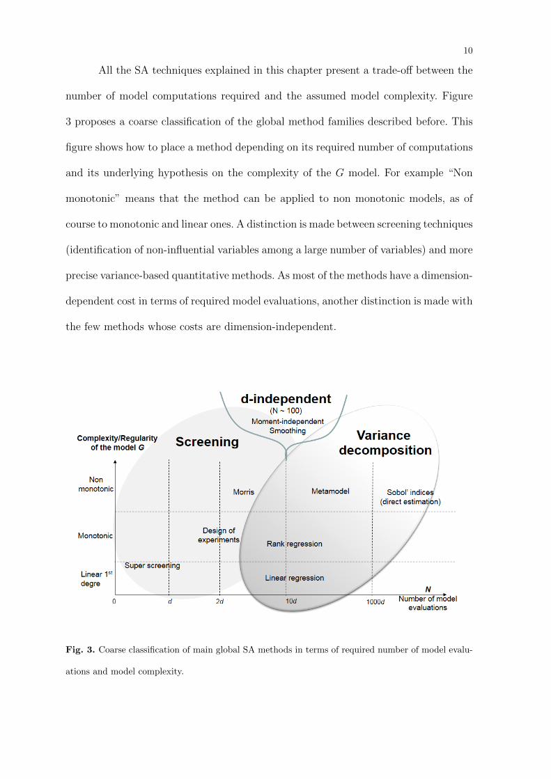
All the SA techniques explained in this chapter present a trade-off between the
number of model computations required and the assumed model complexity. Figure
3 proposes a coarse classification of the global method families described before. This
figure shows how to place a method depending on its required number of computations
and its underlying hypothesis on the complexity of the G model. For example “Non
monotonic” means that the method can be applied to non monotonic models, as of
course to monotonic and linear ones. A distinction is made between screening techniques
(identification of non-influential variables among a large number of variables) and more
precise variance-based quantitative methods. As most of the methods have a dimension-
dependent cost in terms of required model evaluations, another distinction is made with
the few methods whose costs are dimension-independent.
Fig. 3. Coarse classification of main global SA methods in terms of required number of model evalu-
ations and model complexity.

11
Fig. 4. Classification of global SA methods in terms of required number of model evaluations and
model complexity.
With the same axes than the previous figure, Figure 4 proposes a more accurate
classification of the classic global SA methods described in the present SA chapter.
Note that this classification is not exhaustive and does not take full account of ongoing
attempts to improve the existing methods. Overall, this classification tool has several
levels of reading:
• positioning methods based on their cost in terms of the number of model calls.
These methods linearly depend on the dimension (number of inputs) for most
of the methods, except for the moment-independent measures (estimated with
given-data approaches), smoothing methods, Sobol-RBD (Random Balance De-
sign), Sobol-RLHS (Replicated Latin Hypercube Sampling) and statistical tests;

12
• positioning methods based on assumptions about model complexity and regu-
larity;
• distinguishing the type of information provided by each method;
• identifying methods which require some prior knowledge about the model be-
havior.
Each of these techniques corresponds to different categories of problems met
in practice. One should use the simplest method that is adapted to the study’s ob-
jectives, the number of numerical model evaluations that can be performed, and the
prior knowledge on the model’s regularity. Each sensitivity analysis should include a
validation step, which helps to understand if another method should be applied, if the
number if model evaluations should be increased, and so on. Based on the characteris-
tics of the different methods, some authors [9], [26] have proposed decision trees to help
the practitioner to choose the most appropriate method for their problem and model.
Finally, the different papers of this chapter use the same mathematical notations,
which are summarized below:
13
G(·) Numerical model
N , n Sample sizes
d Dimension of an input vector
p Dimension of an output vector
x = (x1, . . . , xd) Deterministic input vector
X = (X1, . . . , Xd) Random input vector
xj, Xj Deterministic and random input variable
xT Transpose of x
x∼i = x−i = xi = (X1, . . . , Xi−1, Xi+1, . . . , Xd)
x(i) Sample vector of x
y, Y ∈ R Deterministic and random output variable when p = 1
y(i) Sample of y
fX(·) Density function of a real random variable X
FX(·) Distribution function of X
µX , σX Mean and standard deviation of X
xα = qα(X) α-quantile of X
V = Var(Y ) Total variance of the model output Y
A Subset of indices in the set {1, . . . , d}
VA Partial variance
SA, StotA First order and total Sobol indices of A
Specialized R software packages
From a practical point of view, the application of SA methods by researchers, engineers,
end-users and students is conditioned by the availability of an easy-to-use software.
Several software include some SA methods (see the Software chapter of the Springer
Handbook) but only a few are specialized on the SA issues. In this section, the sensitivity

14
package of the R environment is presented [49]. Its development has started since 2006
and the several contributions that this package has received have made it particularly
complete. It includes most of the methods presented in the papers of this chapter.
The R software is a powerful tool for knowledge diffusion in the statistical com-
munity. The open source and availability have made R the software of choice for many
statisticians in education and industry. The characteristics of R are the following:
• R is easy to run and install on main operating systems. It can be efficiently used
with an old computer, with a single workstation and with one of the most recent
supercomputer;
• R is a programming language which is interpreted and object-oriented, and
which contains vector operators and matrix computation;
• The main drawbacks of R are its virtual memory limits and non-optimized
computation times. To overcome these problems, compiled languages as fortran
or C are much more efficient, and can be introduced as compiled codes inside R
algorithms requiring huge computation time.
• R contains a lot of built-in statistical functions;
• R is extremely well-documented with built-in help system;
• R encourages the collaboration, the discussion forums and the creation of new
packages by researchers and students. Thousands of packages are made available
on the CRAN website (http://cran.r-project.org/).
All these benefits highlight the interest to develop specific softwares in R and
many packages have been developed on SA. For instance, the FME package contains
basic SA and local SA methods (see Variational Methods), while the spartan package
contains basic methods for exploring stochastic numerical models.

15
For global SA, The sensitivity package includes a collection of functions for factor
screening, sensitivity indices estimation and reliability sensitivity analysis of model
outputs. It implements:
• A few screening techniques as the sequential bifurcations and the Morris method
(see Design of Experiments for Screening). Note that the R package planor allows
to build fractional factorial design (see Design of Experiments for Screening);
• The main sampling-based procedures as linear regression coefficients, partial
correlations, rank transformation (see Weights and Importance in Composite
Indicators: Mind the Gap). Note that the ipcp function of the R package iplots
provides an interactive cobweb graphical tool (see Figure 2), while the R package
CompModSA implements various nonparametric regression procedures for SA
(see Weights and Importance in Composite Indicators: Mind the Gap);
• The variance-based sensitivity indices (Sobol’ indices), by various schemes of the
so-called pick-freeze method, the Extended-FAST method and the replicated
orthogonal array-based Latin hypercube sample (see Variance-based Sensitivity
Analysis: Theory and Estimation Algorithms). The R package fast is fully de-
voted to the FAST method;
• The Poincare constants for the Derivative-based Global Sensitivity Measures
(DGSM) (see Derivative based Global Sensitivity Measures);
• The sensitivity indices based on Csiszar f-divergence and Hilbert-Schmidt In-
dependence Criterion of Da Veiga [6] (see Moment Independence Importance
Measures and a Common Rationale);
• The reliability sensitivity analysis by the Perturbation Law-based Indices (PLI)
(see Moment Independence Importance Measures and a Common Rationale);
• The estimation of the Sobol’ indices with a Gaussian process metamodel
(see Metamodel-based Sensitivity Analysis: Polynomial Chaos and Gaussian
16
Process) with a Gaussian process metamodel coming from the R package DiceK-
riging. Note that the R package tgp performs the same job using treed Gaus-
sian process and that the R package GPC allows to estimate the Sobol’ indices
by building a polynomial chaos metamodel (see Metamodel-based Sensitivity
Analysis: Polynomial Chaos and Gaussian Process);
• Sobol’ indices for multidimensional outputs: Aggregated Sobol’ indices and func-
tional (1D) Sobol’ indices (see Sensitivity Analysis of Spatial and/or Temporal
Phenomena). Note that the R package multisensi is fully devoted to this subject
while the R package safi implements new SA methods of models with functional
inputs;
• The Distributed Evaluation of Local Sensitivity Analysis (DELSA) described in
Rakovec et al [50].
The sensitivity package has been designed to work either models written in R
than external models such as heavy computational codes. This is achieved with the
input argument model present in all functions of this package. The argument model is
expected to be either a function or a predictor (i.e. an object with a predict function
such as lm). The model is invoked once for the whole design of experiment. The argu-
ment model can be left to NULL. This is referred to as the decoupled approach and
used with external computational codes that rarely run on the statistician’s computer.
Examples of use of all the sensitivity functions can be found using the R built-in help
system.
As a global and generic platform allowing to include all the methods of these
different R packages, the mtk package [70] has recently been proposed. It is an object-
oriented framework which aims at dealing with external simulation platforms and man-
aging all the different tasks of uncertainty and sensitivity analyses. Finally, the ATmet

17
and pse packages interface several sensitivity package functions for, respectively, metrol-
ogy applications and parameter space exploration.
Sensitivity auditing
It may happen that a sensitivity analysis of a model-based study is meant to underpin
an inference, and to certify its robustness, in a context where the inference feeds into a
policy or decision making process. In these cases the framing of the analysis itself, its
institutional context, and the motivations of its author may become a matter of great
importance, and a pure SA - with its emphasis on parametric uncertainty - may be seen
as insufficient. The emphasis on the framing may derive inter-alia from the relevance
of the policy study to different constituencies that are characterized by different norms
and values, and hence by a different story about ‘what the problem is’ and foremost
about ‘who is telling the story’. Most often the framing includes more or less implicit
assumptions, which could be political (e.g. which group needs to be protected) all the
way to technical (e.g. which variable can be treated as a constant).
These concerns about how the story is told and who tells it are all the more
urgent in a climate as today’s where science’s own quality assurance criteria are under
scrutiny due to a systemic crisis in reproducibility [25] and the explosion of the blo-
gosphere invites more open debates on the scientific basis of policy decisions [42]. The
Economist, a weekly magazine, has entered the fray by commenting on the poor state of
current scientific practices and devoting its cover to “How Science goes wrong”. It adds
that, ‘The false trails laid down by shoddy research are an unforgivable barrier to under-
standing’ (The Economist [66], p. 11). Among the possible causes of such a predicament
is a process of hybridization [33] of fact and values, and of public and private institu-
tions and actors. Thus the classical division of roles among science, providing tested
fact, and policy, providing legitimized norms, becomes arduous to maintain.

18
As an additional difficulty, according to Grundmann [19], ‘One might suspect
that the more knowledge is produced in hybrid arrangements, the more the protagonists
will insist on the integrity, even veracity of their findings’.
In order to take these concerns into due consideration the instruments of SA have
been extended to provide an assessment of the entire knowledge and model generating
process. This approach has been called sensitivity auditing. It takes inspiration from
NUSAP, a method used to qualify the worth of quantitative information with the
generation of ‘Pedigrees’ of numbers [17], [69]. Likewise, sensitivity auditing has been
developed to provide pedigrees of models and model-based inferences [61], [53], [54].
Sensitivity auditing has been especially designed for an adversarial context,
where not only the nature of the evidence, but also the degree of certainty and uncer-
tainty associated to the evidence, will be the subject of partisan interests. Sensitivity
auditing is structured along a set of seven rules/imperatives:
1. Check against the rhetorical use of mathematical modeling. Question addressed: is
the model being used to elucidate or to obfuscate?;
2. Adopt an ‘assumption hunting’ attitude. Question addressed: what was ‘assumed
out’? What are the tacit, pre-analytical, possibly normative assumptions underlying
the analysis?;
3. Detect Garbage In Garbage Out (GIGO). Issue addressed: artificial deflation of
uncertainty operated in order to achieve a desired inference at a desired level of
confidence. It also works on the reverse practice, the artificial inflation of uncertain-
ties, e.g. to deter regulation;
4. Find sensitive assumptions before they find you. Issue addressed: anticipate crit-
icism by doing careful homework via sensitivity and uncertainty analyses before
publishing results.

19
5. Aim for transparency. Issue addressed: stakeholders should be able to make sense
of, and possibly replicate, the results of the analysis;
6. Do the right sums, which is more important than ‘Do the sums right’. Issue ad-
dressed: is the viewpoint of a relevant stakeholder being neglected? Who decided
that there was a problem and what the problem was?
7. Focus the analysis on the key question answered by the model, exploring the entire
space of the assumptions holistically. Issue addressed: don’t perform perfunctory
analyses that just ‘scratch the surface’ of the system’s potential uncertainties.
The first rule looks at the instrumental use of mathematical modeling to ad-
vance one’s agenda. This use is called rhetorical, or strategic, like the use of Latin by
the elites and clergy before the Reformation. At times the use of models is driven a
simple pursuit of profit; according to Stiglitz [64], this was the case for the modelers
‘pricing’ the derivatives at the root of the sub-prime mortgages crisis:
[. . . ] Part of the agenda of computer models was to maximize the fraction of, say,
a lousy sub-prime mortgage that could get an AAA rating, then an AA rating,
and so forth, [. . . ] This was called rating at the margin, and the solution was still
more complexity, p. 161.
At times this use of models can be called ‘ritual’, in the sense that it offers a false
sense of reassurance. An example is Fisher [13] (quoting Szenberg [65]):

20
Kenneth Arrow, one of the most notable Nobel Laureates in economics, has his
own perspective on forecasting. During World War II, he served as a weather
officer in the U.S. Army Air Corps and worked with a team charged with the
particularly difficult task of producing month-ahead weather forecasts. As Arrow
and his team reviewed these predictions, they confirmed statistically what you
and I might just as easily have guessed: The Corps’ weather forecasts were no
more useful than random rolls of a die. Understandably, the forecasters asked
to be relieved of this seemingly futile duty. Arrow’s recollection of his superiors’
response was priceless: “The commanding general is well aware that the forecasts
are no good. However, he needs them for planning purposes” Szenberg [65].
The second rule about ‘assumption hunting’ is a reminder to look for what
was assumed when the model was originally framed. Modes are full of caeteris paribus
assumptions, meaning that e.g. in economics the model can predict the result of a
shock to a given set of equations assuming that all the rest - all other input variables
and inputs - remains equal, but in real life caeteris are never paribus, meaning by this
that variables tend to be linked with one another, so that they can hardly change in
isolation.
Furthermore at times the assumption made by modelers do not to withstand
scrutiny. A good example of assumption hunting is from John Kay [28], where the
author takes issue with modeling used in transport policy. This author discovered
that among the input values assumed (and hence fixed) in the model was ‘average
car occupancy rates, differentiated by time of day, in 2035’. The point is that such
assumptions are very difficult to justify. This comment was published in the Financial
Times (where John Kay is a columnist) showing that at present times controversies
that could be called epistemological evade the confines of academia and populate the
media.
21
Rule three is about artificially exaggerating or playing down uncertainties wher-
ever convenient. The tobacco lobbies exaggerated the uncertainties about the health
effects of smoking according to Oreskes and Conway [44], while advocates of the death
penalty played down the uncertainties in the negative relations between capital pun-
ishment and crime rate [34]. Clearly the latter wanted the policy, in this case the death
penalty, and were interested in showing that the supporting evidence was robust. In the
former case the lobbies did not want regulation (e.g. bans on tobacco smoking in public
places) and were hence interested in amplifying the uncertainty in the smoking-health
effect causality relationship.
Rule four is about ‘confessing’ uncertainties before going public with the anal-
ysis. This rule is also one of the commandments of applied econometrics according to
Kennedy [29]: ‘Thou shall confess in the presence of sensitivity. Corollary: Thou shall
anticipate criticism’. According to this rule a sensitivity analysis should be performed
before the result of a modeling study are published. There are many good reasons
for doing this, one being that a carefully performed sensitivity analysis often uncovers
plain coding mistakes or model inadequacies. The other is that most often than not
the analysis reveal uncertainties that are larger than those anticipated by the model
developers. Econometrician Edward Leamer in discussing this [34] argues that ‘One
reason these methods are rarely used is their honesty seems destructive’. In Saltelli and
d’Hombres [52], the negative consequences of doing a sensitivity analysis a-posteriori
are discussed. The case is the first review of the cost of offsetting climate change done
by Nicholas Stern of the London School of Economics (the so called Stern Review)
which was criticized by William Nordhaus, of the University of Yale, on the basis of
large sensitivity of the estimates upon the discount factors employed by Stern. Sterns
own sensitivity analysis, published as an annex to the review, revealed according to
the authors in Saltelli and d’Hombres [52] that while the discount factors were not

22
the only important factors determining the cost estimate, the estimates were indeed
very uncertain. On the large uncertainties of integrated assessment models of climate’s
impact, see also Saltelli et al [62].
Rule five is about presenting the results of the modeling study in a transparent
fashion. Both rules originate from the practice of impact assessment, where a modeling
study presented without a proper SA, or as originating from a model which is in fact
a black box, may end up being rejected by stakeholders [52]. Both rules four and five
suggest that reproducibility may be a condition for transparency and that this latter
may be a condition for legitimacy. This debate on Sciences transparency is very much
alive in the US, in the dialectic relationship between the US Environmental Protection
Agency (EPA) and the US Congress (especially the Republican Party) which objects
to EPAs regulations on the basis that these are based on ‘secret science’.
Rule six, about doing the right sum, is not far from the ‘assumptions hunting’
rule; it is just more general. It deals with the fact that often an analyst is set to work
on an analysis arbitrarily framed to the advantage of a party. Sometime this comes via
the choice of the discipline selected to do the analysis. Thus an environmental impact
problem may be framed through the lenses of economics, and presented as a cost benefit
or risk analysis, while the issue has little to do with costs or benefits or risks and a
lot to do with profits, controls, and norms. An example is in Marris et al [41] on the
issue of GMOs, mostly presented in the public discourse as a food safety issue while
the spectrum of concerns of GMO opponents - including lay citizens - appears broader.
According to Winner [71] (p. 138-163), ecologists should not be led into the trap of
arguing about the ‘safety’ of a technology after the technology has been introduced.
They should instead question the broader power, policy and profit implications of that
introduction and its desirability.

23
Rule seven is about avoiding perfunctory sensitivity analyses. As discussed in
Saltelli et al [60], an SA where each uncertain input is moved at a time while leaving all
other inputs fixed is perfunctory. A true SA should make an honest effort at activating
all uncertainties simultaneously, leaving the model free to display its full nonlinear and
possibly non-additive behaviour. A similar point is made in Sam L. Savage’s book ‘The
flaw of averages’ [63].
In conclusion, these rules are meant to help an analyst to anticipate criticism.
In drafting these rules the authors in [61], [53], [54] have tried to put themselves in the
shoes of a modeler also based on their own experience and tried to imagine a model-
based inference feeding into an impact assessment. What questions and objections may
be received by the modeler? Here is a possible list:
• “You treated X as a constant when we know it is uncertain by at least 30%”
• “It would be sufficient for a 5% error in X to make your statement about Z
fragile”
• “Your model is but one of the plausible models - you neglected model uncer-
tainty”
• “ You have instrumentally maximized your level of confidence in the results”
• “Your model is a black box - why should I trust your results?”
• “You have artificially inflated the uncertainty”
• “Your framing is not socially robust”
• “You are answering the wrong question”
The reader may easily check that a careful go through the sensitivity auditing checklist
should provide ammunition to anticipate objections of this nature.
Sensitivity auditing can then be seen as a user guide to criticize the model-based
studies and SA is a part of this guide. In the following section, we go back to sensitivity
analysis in order to conclude and give some perspectives.

24
Conclusion
This introductory paper has presented the SA aims and objectives, the SA and sensitiv-
ity auditing basic principles, the different methods explained in the chapter papers by
positioning them in a classification grid, useful R software packages and the notations
used in the chapter papers. The chapter’s Editor, Bertrand Iooss, would like to sin-
cerely thank all authors and co-authors of the “Sensitivity Analysis” chapter for their
efforts and the quality of their contributions. Dr. Jean-Philippe Argaud (EDF R&D),
Dr. Geraud Blatman (EDF R&D), Dr. Nicolas Bousquet (EDF R&D), Dr. Sebastien da
Veiga (Safran), Dr. Herve Monod (INRA), Dr. Matieyendou Lamboni (INRA) and Dr.
Loıc Le Gratiet (EDF R&D) are also greatly thanked for their advices on the different
chapter papers.
The papers in this chapter the most widely used methods for sensitivity analy-
sis: the deterministic methods as the local sensitivity analysis, the experimental design
strategies, the sampling-based and variance-based methods developed from the 1980s
and the new importance measures and metamodel-based techniques established and
studied since the 2000s. However, with such a rich subject, choices had to be made for
the different chapter papers and some important omissions are present. For instance,
the robust Bayesian analysis [1], [24] is not discussed, while it is nevertheless a great
ingredient in the study of the sensitivity of Bayesian answers to assumptions and uncer-
tain calculation inputs. Moreover, in the context of non-probabilistic representation of
uncertainty (as in the interval analysis, the evidence theory and the possibility theory),
a small amount of SA methods has been developed [22]. This subject is deferred to a
future review work.
Due to their very new or incomplete nature, several other SA issues are not
discussed in this chapter. For instance, estimating total Sobol’ indices at low cost re-
mains a problem of primary importance in many applications (see Saltelli et al [60] for

25
a recent review on the subject). Second-order Sobol indices estimations have recently
been considered by Fruth et al [16] (by way of total interaction indices) and Tissot
and Prieur [67] (by way of replicated orthogonal-array LHS). The latter work offers a
powerful estimation method because the number of model calls is independent of the
number of inputs (as in the spirit of permutation-based technique [38], [37]). However,
for high-dimensional models (several hundreds inputs), estimation biases and computa-
tional costs remain considerable; De Castro and Janon [8] have proposed to introduce
modern statistical techniques based on variable selection in regression models. Owen
[46] has introduced generalized Sobol’ indices allowing to compare and search efficient
estimators (as the new one found in Owen [45]).
Another mathematical difficulty is the consideration of the dependence between
the inputs Xi (i = 1 . . . d). Non-independence between inputs in SA has been discussed
by many authors such as Saltelli and Tarantola [55], Jacques et al [27], Xu and Gertner
[72], Da Veiga et al [7], Li et al [36], Kucherenko et al [31], Mara and Tarantola [39]
and Chastaing et al [5]. Despite all these works, much confusion still exists in practical
applications. In practice, it would be useful to be able to measure the influence of the
potential dependence between some inputs on the output quantity of interest.
Note that most of the works in this chapter focus on SA relative to the overall
variability of model output (second order statistics). In practice, one can be interested in
other quantities of interest, such as the output entropy, the probability that the output
exceeds a threshold and a quantile estimation [56], [15], [35]. This is an active area of
research as shown in this chapter (see Moment Independence Importance Measures and
a Common Rationale), but innovative and powerful ideas have recently been developed
by Owen et al [47] and Geraci et al [18] using higher order statistics, Fort et al [14]
using contrast functions and Da Veiga [6] using a kernel point of view.
26
Finally, in some situations, the computer code is not a deterministic simulator
but a stochastic one. This means that two model calls with the same set of input
variables lead to different output values. Typical stochastic computer codes are queuing
models, agent-based models, and models involving partial differential equations applied
to heterogeneous or Monte Carlo-based numerical models. For this type of code, Marrel
et al [40] have proposed a first solution for dealing with Sobol’ indices. Moutoussamy
et al [43] have also tackled the issue in the context of the metamodel building of the
output probability density function. Developing relevant SA methods in this context
will certainly be subject of future works.
References
1. Berger J (1994) An overview of robust Bayesian analysis (with discussion). Test 3:5–124
2. Borgonovo E, Plischke E (2015) Sensitivity analysis: A review of recent advances. European journal
of operational Research, In press
3. Cacuci D (2003) Sensitivity and uncertainty analysis - Theory. Chapman & Hall/CRC
4. Castaings W, Dartus D, Le Dimet FX, Saulnier GM (2009) Sensitivity analysis and parameter
estimation for distributed hydrological modeling : potential of variational methods. Hydrology
and Earth System Sciences Discussions 13:503–517
5. Chastaing G, Gamboa F, Prieur C (2012) Generalized Hoeffding-Sobol decomposition for depen-
dent variables - Application to sensitivity analysis. Electronic Journal of Statistics 6:2420–2448
6. Da Veiga S (2015) Global sensitivity analysis with dependence measures. Journal of Statistical
Computation and Simulation 85:1283–1305
7. Da Veiga S, Wahl F, Gamboa F (2009) Local polynomial estimation for sensitivity analysis on
models with correlated inputs. Technometrics 51(4):452–463
8. De Castro Y, Janon A (2015) Randomized pick-freeze for sparse Sobol indices estimation in high
dimension. ESAIM P&S, In press
9. de Rocquigny E, Devictor N, Tarantola S (eds) (2008) Uncertainty in industrial practice. Wiley

27
10. Dean A, Lewis S (eds) (2006) Screening - Methods for experimentation in industry, drug discovery
and genetics. Springer
11. Faivre R, Iooss B, Mahevas S, Makowski D, Monod H (eds) (2013) Analyse de sensibilite et
exploration de modeles. Editions Quae
12. Fang KT, Li R, Sudjianto A (2006) Design and modeling for computer experiments. Chapman &
Hall/CRC
13. Fisher RW (2011) Remembering Carol Reed, Aesop’s Fable, Kenneth Arrow and Thomas
Dewey. In: Speech: An Economic Overview: What’s Next, Federal Reserve Bank of Dallas,
http://www.dallasfed.org/news/speeches/fisher/2011/fs110713.cfm
14. Fort J, Klein T, Rachdi N (2014) New sensitivity analysis subordinated to a contrast. Communi-
cations in Statistics Theory and Methods, In press
15. Frey H, Patil S (2002) Identification and review of sensitivity analysis methods. Risk Analysis
22:553–578
16. Fruth J, Roustant O, Kuhnt S (2014) Total interaction index: A variance-based sensitivity index
for second-order interaction screening. Journal of Statistical Planning and Inference 147:212–223
17. Funtowicz S, Ravetz J (1990) Uncertainty and Quality in Science for Policy. Kluwer Academic
Publishers, The Netherlands
18. Geraci G, Congedo P, Iaccarino G (2015) Decomposing high-order statistics for sensitivity analysis.
In: Thermal & Fluid Sciences Industrial Affiliates and Sponsors Conference, Stanford University,
Stanford, United States
19. Grundmann R (2009) The role of expertise in governance processes. Forest Policy and Economics
11:398–403
20. Helton J (1993) Uncertainty and sensitivity analysis techniques for use in performance assesment
for radioactive waste disposal. Reliability Engineering and System Safety 42:327–367
21. Helton J (2008) Uncertainty and sensitivity analysis for models of complex systems. In: Graziani F
(ed) Computational methods in transport: Verification and validation, New-York, NY: Springer-
Verlag, pp 207–228
22. Helton J, Johnson J, Obekampf W, Salaberry C (2006) Sensitivity analysis in conjunction with ev-
idence theory representations of epistemic uncertainty. Reliability Engineering and System Safety
91:1414–1434

28
23. Helton J, Johnson J, Salaberry C, Storlie C (2006) Survey of sampling-based methods for uncer-
tainty and sensitivity analysis. Reliability Engineering and System Safety 91:1175–1209
24. Insua D, Ruggeri F (eds) (2000) Robust Bayesian Analysis. Springer-Verlag, New York
25. Ioannidis JPA (2005) Why most published research findings are false. PLoS Medicine 2(8):696–701
26. Iooss B, Lemaıtre P (2015) A review on global sensitivity analysis methods. In: Meloni C, Dellino
G (eds) Uncertainty management in Simulation-Optimization of Complex Systems: Algorithms
and Applications, Springer
27. Jacques J, Lavergne C, Devictor N (2006) Sensitivity analysis in presence of model uncertainty
and correlated inputs. Reliability Engineering and System Safety 91:1126–1134
28. Kay J (2011) A wise man knows one thing - The limits of his knowledge. Financial Times 29
november
29. Kennedy P (2007) A Guide to Econometrics, 5th ed. Blackwell Publishing, Oxford
30. Kleijnen J (1997) Sensitivity analysis and related analyses: a review of some statistical techniques.
Journal of Statistical Computation and Simulation 57:111–142
31. Kucherenko S, Tarantola S, Annoni P (2012) Estimation of global sensitivity indices for models
with dependent variables. Computer Physics Communications 183:937–946
32. Kurowicka D, Cooke R (2006) Uncertainty analysis with high dimensional dependence modelling.
Wiley
33. Latour B (1993) We Have Never Been Modern. Cambridge, Harvard UP
34. Leamer EE (2010) Tantalus on the road to asymptopia. Journal of Economic Perspectives 4(2):31–
46
35. Lemaıtre P, Sergienko E, Arnaud A, Bousquet N, Gamboa F, Iooss B (2015) Density modification
based reliability sensitivity analysis. Journal of Statistical Computation and Simulation 85:1200–
1223
36. Li G, Rabitz H, Yelvington P, Oluwole O, Bacon F, Kolb C, Schoendorf J (2010) Global sensitivity
analysis for systems with independent and/or correlated inputs. Journal of Physical Chemistry
114:6022–6032
37. Mara T (2009) Extension of the RBD-FAST method to the computation of global sensitivity
indices. Reliability Engineering and System Safety 94:1274–1281
38. Mara T, Joseph O (2008) Comparison of some efficient methods to evaluate the main effect of
computer model factors. Journal of Statistical Computation and Simulation 78:167–178
29
39. Mara T, Tarantola S (2012) Variance-based sensitivity indices for models with dependent inputs.
Reliability Engineering and System Safety 107:115–121
40. Marrel A, Iooss B, Da Veiga S, Ribatet M (2012) Global sensitivity analysis of stochastic computer
models with joint metamodels. Statistics and Computing 22:833–847
41. Marris C, Wynne B, P S, , Weldon S (2001) Final report of the PABE research project funded
by the Commission of European Communities. Tech. Rep. Contract number: FAIR CT98-3844
(DG12 - SSMI), Commission of European Communities
42. Monbiot G (2013) Beware the rise of the government scientists turned lobbyists. The Guardian
29 april
43. Moutoussamy V, Nanty S, Pauwels B (2015) Emulators for stochastic simulation codes. ESAIM:
PROCEEDINGS AND SURVEYS 48:116–155
44. Oreskes N, Conway EM (2010) Merchants of Doubt: How a Handful of Scientists Obscured the
Truth on Issues from Tobacco Smoke to Global Warming. Bloomsbury Press, New York
45. Owen A (2013) Better estimation of small Sobol’ sensitivity indices. ACM Transactions on Mod-
eling and Computer Simulation 23:11
46. Owen A (2013) Variance components and generalized Sobol’ indices. Journal of Uncertainty Quan-
tification 1:19–41
47. Owen A, Dick J, Chen S (2014) Higher order Sobol’ indices. Information and Inference: A Journal
of the IMA 3:59–81
48. Park K, Xu L (2008) Data assimilation for atmospheric, oceanic and hydrologic applications.
Springer
49. Pujol G, Iooss B, Janon A (2015) sensitivity package, version 1.11. The Comprenhensive R Archive
Network, URL http://www.cran.r-project.org/web/packages/sensitivity/
50. Rakovec O, Hill MC, Clark MP, Weerts AH, Teuling AJ, Uijlenhoet R (2014) Distributed Eval-
uation of Local Sensitivity Analysis (DELSA), with application to hydrologic models. Water Re-
sources Research 50:1–18
51. Saltelli A (2002) Making best use of model evaluations to compute sensitivity indices. Computer
Physics Communication 145:280–297
52. Saltelli A, d’Hombres B (2010) Sensitivity analysis didn’t help. A practitioners critique of the
Stern review. Global Environmental Change 20(2):298–302

30
53. Saltelli A, Funtowicz S (2014) When all models are wrong: More stringent quality criteria are
needed for models used at the science-policy interface. Issues in Science and Technology Winter:79–
85
54. Saltelli A, Funtowicz S (2015) Evidence-based policy at the end of the Cartesian dream: The case
of mathematical modelling. In: Guimares Pereira, Funtowicz S (eds) The end of the Cartesian
dream. Beyond the technoscientific worldview, Routledge’s series: Explorations in Sustainability
and Governance, pp 147–162
55. Saltelli A, Tarantola S (2002) On the relative importance of input factors in mathematical models:
Safety assessment for nuclear waste disposal. Journal of American Statistical Association 97:702–
709
56. Saltelli A, Chan K, Scott E (eds) (2000) Sensitivity analysis. Wiley Series in Probability and
Statistics, Wiley
57. Saltelli A, Tarantola S, Campolongo F (2000) Sensitivity analysis as an ingredient of modelling.
Statistical Science 15:377–395
58. Saltelli A, Tarantola S, Campolongo F, Ratto M (2004) Sensitivity analysis in practice: A guide
to assessing scientific models. Wiley
59. Saltelli A, Ratto M, Andres T, Campolongo F, Cariboni J, Gatelli D, Salsana M, Tarantola S
(2008) Global sensitivity analysis - The primer. Wiley
60. Saltelli A, Annoni P, Azzini I, Campolongo F, Ratto M, Tarantola S (2010) Variance based
sensitivity analysis of model output. Design and estimator for the total sensitivity index. Computer
Physics Communication 181:259–270
61. Saltelli A, Pereira G, Van der Sluijs JP, Funtowicz S (2013) What do I make of your lati-
norum? Sensitivity auditing of mathematical modelling. Int J Foresight and Innovation Policy
9(2/3/4):213–234
62. Saltelli A, Stark P, Becker W, Stano P (2015) Climate models as economic guides. Scientific
challenge or quixotic quest? Issues in Science and Technology XXXI(3)
63. Savage SL (2009) The Flaw of Averages: Why We Underestimate Risk in the Face of Uncertainty.
Wiley
64. Stiglitz J (2010) Freefall, Free Markets and the Sinking of the Global Economy. Penguin, London
65. Szenberg (1992) Eminent Economists: Their Life Philosophies. Cambridge, England: Cambridge
University Press

31
66. The Economist (2013) How science goes wrong. The Economist 19 october
67. Tissot JY, Prieur C (2015) A randomized Orthogonal Array-based procedure for the estimation of
first- and second-order Sobol’ indices. Journal of Statistical Computation and Simulation 85:1358–
1381
68. Turanyi T (1990) Sensitivity analysis for complex kinetic system, tools and applications. Journal
of Mathematical Chemistry 5:203–248
69. Van der Sluijs JP, Craye M, Funtowicz S, Kloprogge P, Ravetz J, Risbey J (2005) Combining
quantitative and qualitative measures of uncertainty in model based environmental assessment:
the NUSAP system. Risk Analysis 25(2):481–492
70. Wang J, Faivre R, Richard H, Monod H (2015) mtk (Mexico Toolkit): An R package for uncertainty
and sensitivity analyses of numerical experiments. The R Journal, In press
71. Winner L (1989) The Whale and the Reactor: a Search for Limits in an Age of High Technology.
The University of Chicago Press, Chicago
72. Xu C, Gertner G (2007) Extending a global sensitivity analysis technique to models with correlated
parameters. Computational Statistics and Data Analysis 51:5579–5590