Embed Size (px)
DESCRIPTION
a detailed report
Citation preview

1/45
Introduction Robotics
Introduction Robotics, lecture 4 of 7
dr Dragan Kostić
WTB Dynamics and Control
September - October 2009
Introduction Robotics

2/45
• Recapitulation
• Velocity kinematics
Outline
Introduction Robotics, lecture 4 of 7
• Manipulator Jacobian
• Kinematic singularities
• Inverse velocity kinematics

3/45
Recapitulation
Introduction Robotics, lecture 4 of 7
Recapitulation
4/45
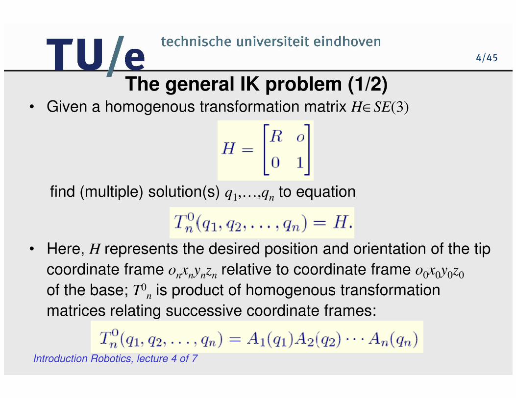
The general IK problem (1/2)• Given a homogenous transformation matrix H∈SE(3)
find (multiple) solution(s) q1,…,qn to equation
Introduction Robotics, lecture 4 of 7
find (multiple) solution(s) q1,…,qn to equation
• Here, H represents the desired position and orientation of the tip
coordinate frame onxnynzn relative to coordinate frame o0x0y0z0
of the base; T0n is product of homogenous transformation
matrices relating successive coordinate frames:

5/45
The general IK problem (2/2)
• Since the bottom rows of both T0n and H are equal to [0 0 0 1],
equation
Introduction Robotics, lecture 4 of 7
gives rise to 4 trivial equations and 12 equations in n unknowns
q1,…,qn:
Here, Tij and Hij are nontrivial elements of T0n and H.
6/45
Kinematic decoupling (1/3)
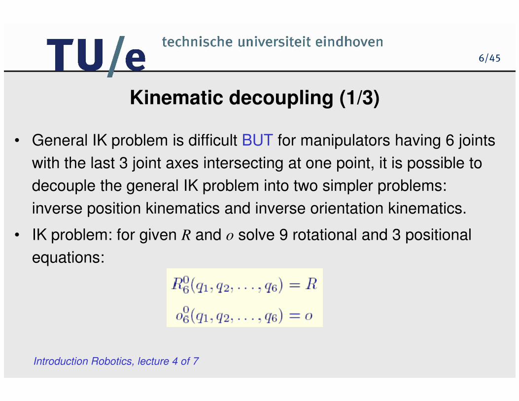
• General IK problem is difficult BUT for manipulators having 6 joints
with the last 3 joint axes intersecting at one point, it is possible to
decouple the general IK problem into two simpler problems:
inverse position kinematics and inverse orientation kinematics.
Introduction Robotics, lecture 4 of 7
inverse position kinematics and inverse orientation kinematics.
• IK problem: for given R and o solve 9 rotational and 3 positional
equations:

7/45
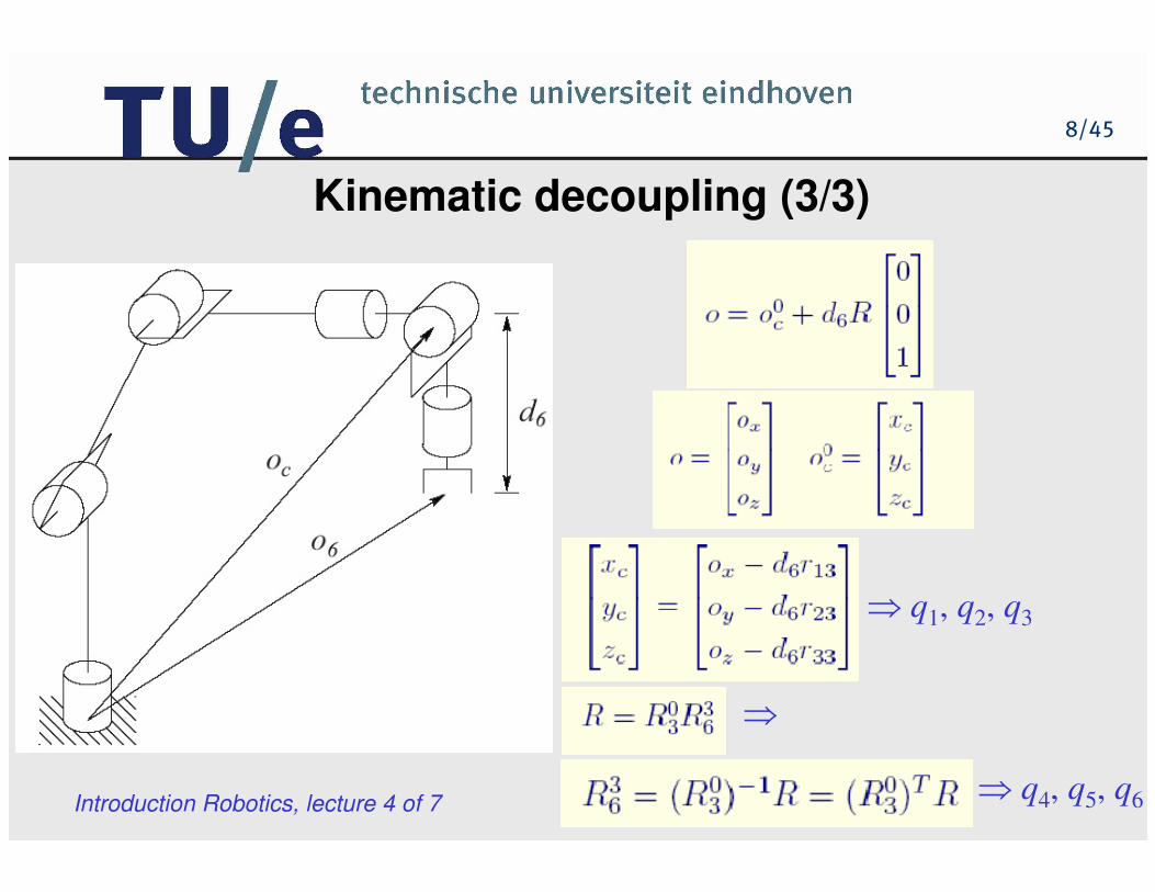
Kinematic decoupling (2/3)
• Spherical wrist as paradigm.
Introduction Robotics, lecture 4 of 7
• Let oc be the intersection of the last 3 joint axes; as z3, z4, and z5
intersect at oc, the origins o4 and o5 will always be at oc;
the motion of joints 4, 5 and 6 will not change the position of oc;
only motions of joints 1, 2 and 3 can influence position of oc.
8/45
Kinematic decoupling (3/3)
Introduction Robotics, lecture 4 of 7
⇒ q1, q2, q3
⇒
⇒ q4, q5, q6

9/45
Introduction Robotics, lecture 4 of 7
Velocity Kinematics

10/45
Scope
• Mathematically, forward kinematics defines a function between
the space of joint positions and the space of Cartesian positions
and orientations of a robot tip; the velocity kinematics are then
Introduction Robotics, lecture 4 of 7
determined by the Jacobian of this function.
• Jacobian is encountered in many aspects of robotic manipulation:
in the planning and execution of robot trajectories, in the
derivation of the dynamic equations of motion, etc.
11/45
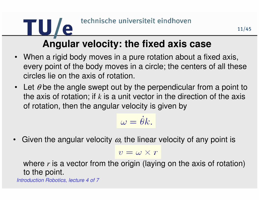
Angular velocity: the fixed axis case
• When a rigid body moves in a pure rotation about a fixed axis,
every point of the body moves in a circle; the centers of all these
circles lie on the axis of rotation.
• Let θ be the angle swept out by the perpendicular from a point to the axis of rotation; if k is a unit vector in the direction of the axis
Introduction Robotics, lecture 4 of 7
the axis of rotation; if k is a unit vector in the direction of the axis
of rotation, then the angular velocity is given by
• Given the angular velocity ω, the linear velocity of any point is
where r is a vector from the origin (laying on the axis of rotation)to the point.
12/45
Skew symmetric matrices
• An n × n matrix S is skew symmetric if and only if
• The set of all such matrices is denoted by so(n).
Introduction Robotics, lecture 4 of 7
• From this definition, we see that the diagonal elements of S
are zero, i.e. sii = 0; also, we see that S ∈ so(3) contains
only 3 independent entries and has the form
13/45
Properties of skew symmetric matrices
• For a vector a=[ax, ay, az]T we define
Introduction Robotics, lecture 4 of 7

14/45
The derivative of a rotation matrix
• If R(θ) ∈ SO(3), then R(θ)RT (θ) = I. Differentiating both sides
w.r.t. θ yields
Introduction Robotics, lecture 4 of 7
• Since R(θ)RT (θ) = I , we obtain:
• Multiplying both sides on the right by R and using the fact
that ST = -S, we get
[ ] .0)()()()( =− θθθθθ
SRRRRd
d T
15/45
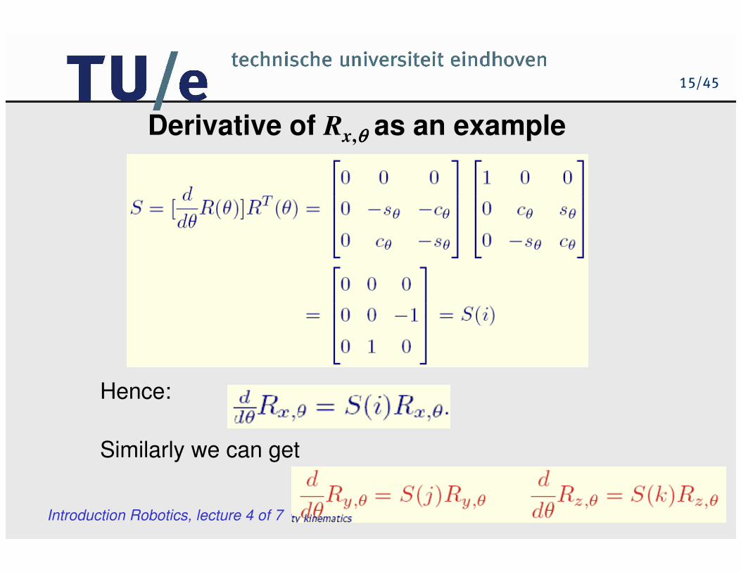
Derivative of Rx,θθθθ as an example
Introduction Robotics, lecture 4 of 7
Hence:
Similarly we can get

16/45
Derivative of Rl,θθθθ
• Let Rl,θ be a rotation matrix about the axis defined by unit vector l.
Then
Introduction Robotics, lecture 4 of 7

17/45
Angular velocity: general case
• Consider angular velocity ω about an arbitrary, possibly moving,
axis. Suppose that R(t) ∈ SO(3) is a time-dependent rotation
matrix. Then
Introduction Robotics, lecture 4 of 7
matrix. Then
where ω(t) is the angular velocity of the rotating frame with respect
to the fixed frame at time t.
18/45
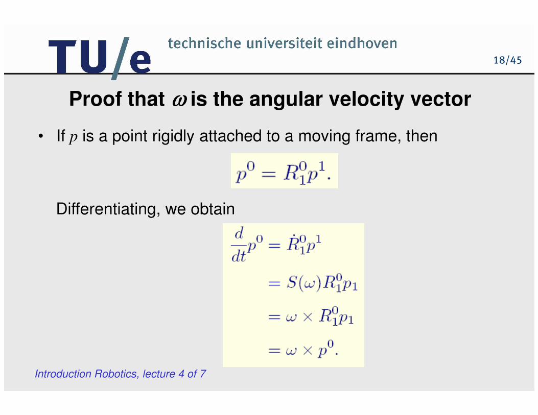
Proof that ωωωω is the angular velocity vector
• If p is a point rigidly attached to a moving frame, then
Differentiating, we obtain
Introduction Robotics, lecture 4 of 7
Differentiating, we obtain
19/45
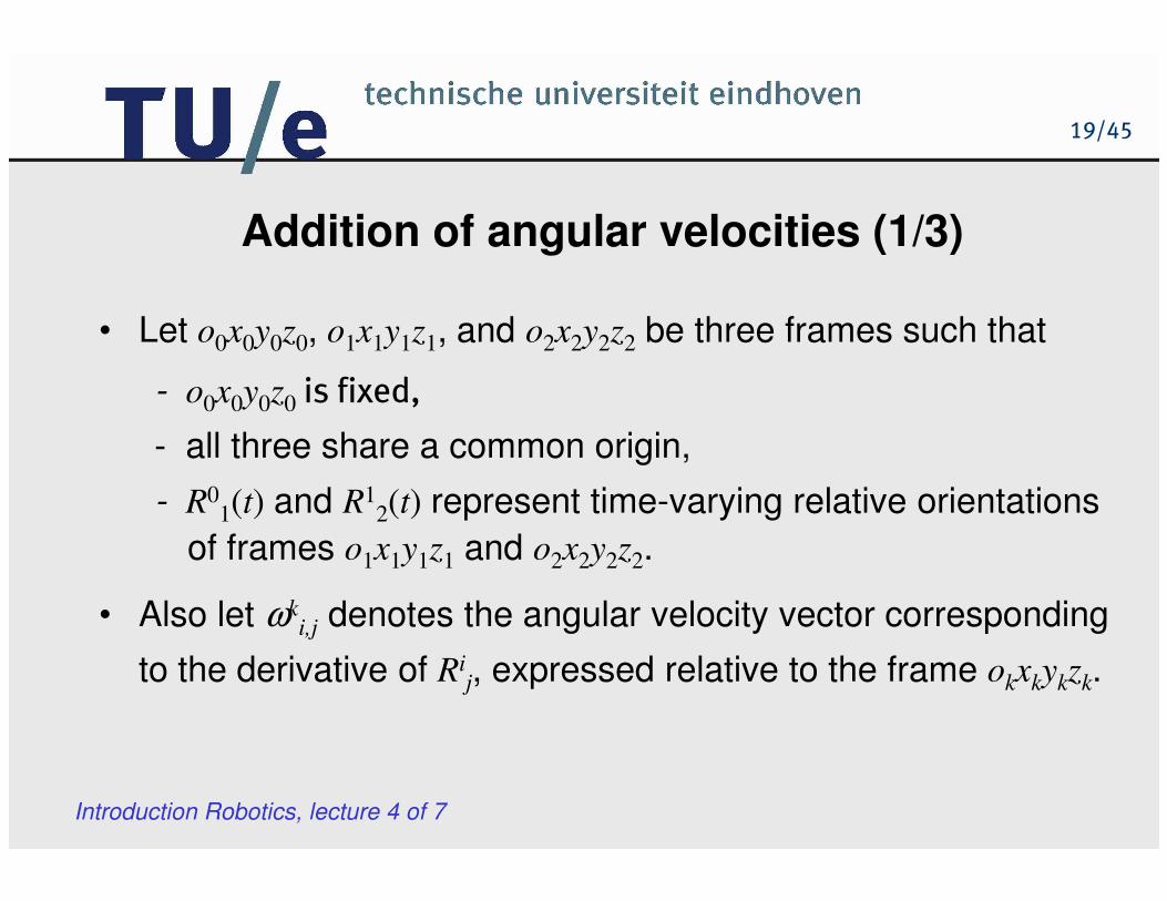
Addition of angular velocities (1/3)
• Let o0x0y0z0, o1x1y1z1, and o2x2y2z2 be three frames such that
- o0x0y0z0 is fixed,
- all three share a common origin,
Introduction Robotics, lecture 4 of 7
- all three share a common origin,
- R01(t) and R1
2(t) represent time-varying relative orientations
of frames o1x1y1z1 and o2x2y2z2.
• Also let ωki,j denotes the angular velocity vector corresponding
to the derivative of Rij, expressed relative to the frame okxkykzk.
20/45
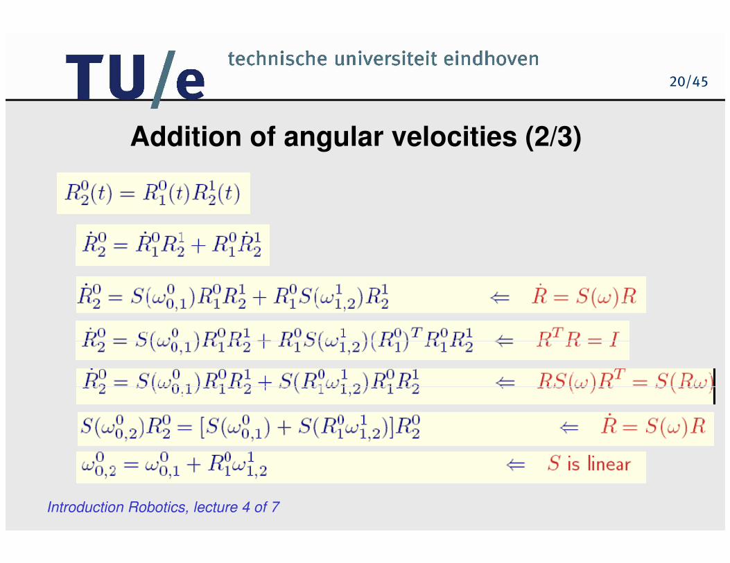
Addition of angular velocities (2/3)
Introduction Robotics, lecture 4 of 7

21/45
Addition of angular velocities (3/3)
• For an arbitrary number of coordinate systems:
Introduction Robotics, lecture 4 of 7

22/45
Linear velocity of a point attached to a moving frame (1/2)
• Suppose that p is rigidly attached to the frame o1x1y1z1 and that
o1x1y1z1 is rotating relative to the frame o0x0y0z0.
• Then, we have
Introduction Robotics, lecture 4 of 7
23/45
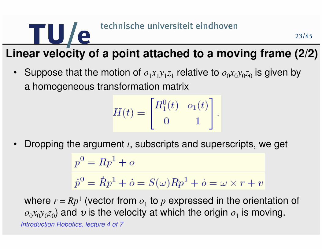
Linear velocity of a point attached to a moving frame (2/2)
• Suppose that the motion of o1x1y1z1 relative to o0x0y0z0 is given by
a homogeneous transformation matrix
Introduction Robotics, lecture 4 of 7
• Dropping the argument t, subscripts and superscripts, we get
where r = Rp1 (vector from o1 to p expressed in the orientation of
o0x0y0z0) and υ is the velocity at which the origin o1 is moving.

24/45
Introduction Robotics, lecture 4 of 7
Manipulator Jacobian

25/45
Derivation of the Jacobian• Consider an n-link manipulator with joint variables q1, q2, …, qn.
• Let q = [q1, q2, …, qn]T.
• Let the transformation from the end-effector to the
base frame be:
Introduction Robotics, lecture 4 of 7
Karl Gustav
Jacob Jacobi
(1804-1851)
• Let the angular velocity of the end-effector ω0n be
• Linear velocity of the end-effector is
• We seek expressions

26/45
The manipulator Jacobian
• The manipulator Jacobian:
Introduction Robotics, lecture 4 of 7
Karl Gustav
Jacob Jacobi
(1804-1851)
27/45
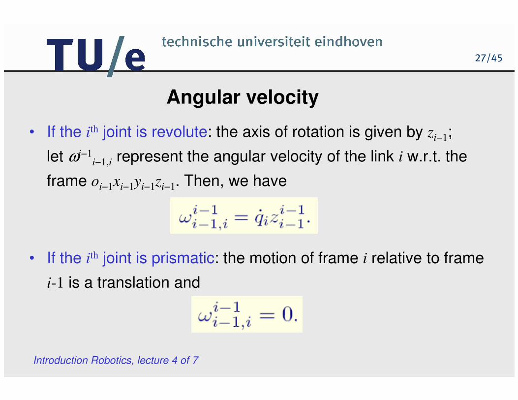
Angular velocity
• If the ith joint is revolute: the axis of rotation is given by zi−1;
let ωi−1i−1,i represent the angular velocity of the link i w.r.t. the
frame oi−1xi−1yi−1zi−1. Then, we have
Introduction Robotics, lecture 4 of 7
• If the ith joint is prismatic: the motion of frame i relative to frame
i-1 is a translation and

28/45
Overall angular velocity
• By using already derived formula
we get
Introduction Robotics, lecture 4 of 7
where
we get
,0
1
0
122
0
011
1
1
0
1
1
1
0
122
0
011
0
,0
−
−−−
+++=
=+++=
nnn
n
nnnnn
zqzqzq
zRqzRqzq
&K&&
&K&&
ρρρ
ρρρω
29/45
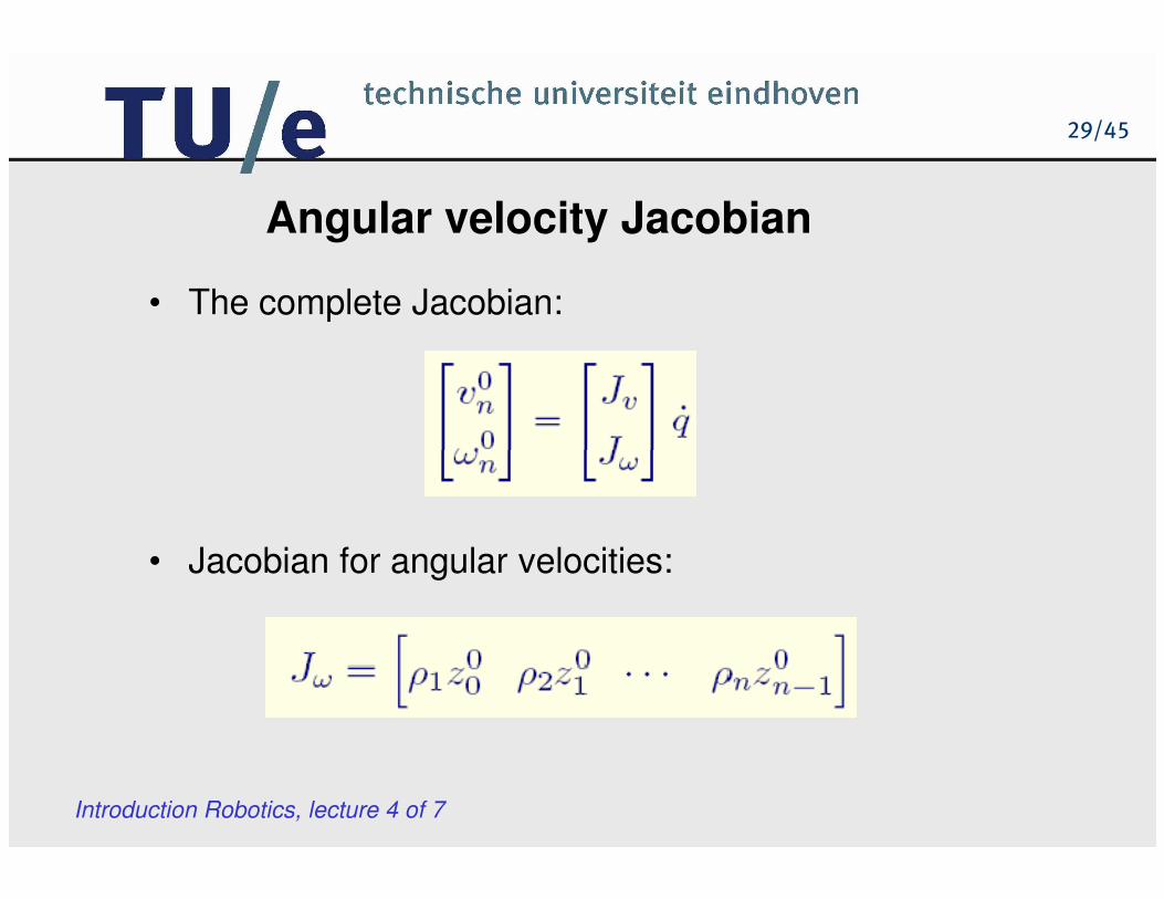
Angular velocity Jacobian
• The complete Jacobian:
Introduction Robotics, lecture 4 of 7
• Jacobian for angular velocities:

30/45
Linear velocity Jacobian
• The linear velocity of the end effector is just
• By the chain rule for differentiation
Introduction Robotics, lecture 4 of 7
• By the chain rule for differentiation
we find Jacobian for linear velocities

31/45
Case 1: prismatic joints
Introduction Robotics, lecture 4 of 7

32/45
Case 2: revolute joints
• The linear velocity of the
end-effector is of form
Introduction Robotics, lecture 4 of 7
where
• Hence we get

33/45
Combining the linear and angular velocity Jacobians
• The Jacobian is given by
where
Introduction Robotics, lecture 4 of 7
where
and
34/45
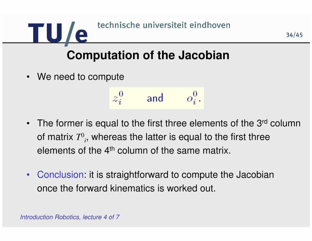
Computation of the Jacobian
• We need to compute
• The former is equal to the first three elements of the 3rd column
Introduction Robotics, lecture 4 of 7
• The former is equal to the first three elements of the 3rd column
of matrix T0i, whereas the latter is equal to the first three
elements of the 4th column of the same matrix.
• Conclusion: it is straightforward to compute the Jacobian
once the forward kinematics is worked out.

35/45
Kinematic singularities
Introduction Robotics, lecture 4 of 7
Kinematic singularities

36/45
Kinematic singularities
• The 6×n manipulator Jacobian J(q) defines mapping
qqJ &)(=ξ
• All possible end-effector velocities are linear combinations of
the columns Ji of the Jacobian
Introduction Robotics, lecture 4 of 7
the columns Ji of the Jacobian
nnqJqJqJ &K&& +++= 2211ξ
• The rank of a matrix is the number of linearly independent
columns (or rows) in the matrix; for J∈RRRR6×n:
),6min(rank nJ ≤
• The rank of Jacobian depends on the configuration q; at singular
configurations, rankJ(q) is less than its maximum value.

37/45
Properties of kinematic singularities
• At singular configurations:
– certain directions of end-effector motion may be unattainable,
– bounded end-effector velocities may correspond to unbounded
joint velocities,
Introduction Robotics, lecture 4 of 7
joint velocities,
– bounded joint torques may correspond to unbounded
end-effector forces and torques.
• Singularities correspond to points:
– on the boundary of the manipulator workspace,
– within the manipulator workspace that may be unreachable under small
perturbations of the link parameters (e.g. length, offset, etc.).

38/45
Examples of kinematic singularities (1/2)
Introduction Robotics, lecture 4 of 7

39/45
Examples of kinematic singularities (2/2)
Introduction Robotics, lecture 4 of 7

40/45
Inverse velocity kinematics
Introduction Robotics, lecture 4 of 7
Inverse velocity kinematics

41/45
Inverse velocity problem
• The Jacobian kinematic relationship:
• The inverse velocity problem is to find joint velocities that produce
the desired end-effector velocity.
Introduction Robotics, lecture 4 of 7
the desired end-effector velocity.
• When Jacobian is square (manipulator has 6 joints) and nonsingular,
one gets:
• If the number of joints is not exactly 6, J cannot be inverted; then the
inverse velocity problem has a solution (obtained using e.g. Gaussian
elimination) if and only if

42/45
Pseudoinverse of Jacobian
• When number of joints n is above 6, the manipulator is
kinematically redundant; then, the inverse velocity problem
can be solved using the pseudoinverse of J.
• Suppose that rank J = m and m<n. Then, the right pseudoinverse
Introduction Robotics, lecture 4 of 7
• Suppose that rank J = m and m<n. Then, the right pseudoinverse
of J is given by
• Note that
• It holds
where b ∈RRRRn is an arbitrary vector.
43/45
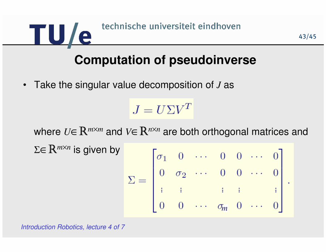
Computation of pseudoinverse
• Take the singular value decomposition of J as
where U∈RRRRm×m and V∈RRRRn×n are both orthogonal matrices and
Introduction Robotics, lecture 4 of 7
where U∈RRRRm×m and V∈RRRRn×n are both orthogonal matrices and
Σ∈RRRRm×n is given by
m

44/45
Formula for pseudoinverse
• The right pseudoinverse of J is
where
Introduction Robotics, lecture 4 of 7
where
T
m

45/45
Measures of kinematic manipulability
• Indicate how close is manipulator to a singular configuration.
• In terms of singular values σi of the manipulator Jacobian J,
kinematic manipulability is defined by:
σσσµ ⋅⋅⋅= L
Introduction Robotics, lecture 4 of 7
mσσσµ ⋅⋅⋅= L21
• In terms of eigenvalues λi of J or determinant of J, µ is given by:
mT
JJ λλλµ ⋅⋅⋅== L21det
• Condition number of J is another manipulability measure:
.,,1;min
maxcond miJ
i
iL==
σ
σ