Embed Size (px)
Citation preview

CAVALIERI INTEGRATION
T. L. GROBLER†, E. R. ACKERMANN‡, A. J. VAN ZYL#, AND J. C. OLIVIER?
Abstract. We use Cavalieri’s principle to develop a novel integration tech-
nique which we call Cavalieri integration. Cavalieri integrals differ from Rie-
mann integrals in that non-rectangular integration strips are used. In thisway we can use single Cavalieri integrals to find the areas of some interesting
regions for which it is difficult to construct single Riemann integrals.
We also present two methods of evaluating a Cavalieri integral by firsttransforming it to either an equivalent Riemann or Riemann-Stieltjes integral
by using special transformation functions h(x) and its inverse g(x), respec-
tively. Interestingly enough it is often very difficult to find the transformationfunction h(x), whereas it is very simple to obtain its inverse g(x).
1. Introduction
We will use Cavalieri’s principle to develop a novel integration technique whichcan be used to almost effortlessly find the area of some interesting regions for whichit is rather difficult to construct single Riemann integrals. We will call this typeof integration Cavalieri integration. As the name suggests, Cavalieri integration isbased on the well known Cavalieri principle, stated here without proof [3]:
Theorem 1.1 (Cavalieri’s principle). Suppose two regions in a plane are includedbetween two parallel lines in that plane. If every line parallel to these two linesintersects both regions in line segments of equal length, then the two regions haveequal areas.
∆x ∆x
A B
Figure 1. Simple illustration of Cavalieri’s principle in R2, witharea A = area B.
Inspired by Cavalieri’s principle, we pose the following question: what happenswhen we replace the usual rectangular integration strip of the Riemann sum withan integration strip that has a non-rectangular shape? It turns out that such aformulation leads to a consistent scheme of integration with a few surprising results.
1991 Mathematics Subject Classification. Primary 26A42.Key words and phrases. Cavalieri; method of indivisibles; integration; Riemann; Riemann-
Stieltjes.
1

2 T. L. GROBLER†, E. R. ACKERMANN‡, A. J. VAN ZYL#, AND J. C. OLIVIER?
By considering non-rectangular integration strips we form a Cavalieri sum whichcan either be transformed to a normal Riemann sum (of an equivalent region) byusing a transformation function h(x), or to a Riemann-Stieltjes sum by using theinverse transformation function g(x).
The main result of Cavalieri integration can be demonstrated by using a simpleexample. Consider the region bounded by the x-axis and the lines f(x) = x,a(y) = 1− y and b(y) = 4− y, shown in Figure 2.A. Notice that we cannot expressthe area of this region as a single Riemann integral. We can however calculate thearea of this region by using a single Cavalieri integral:
Area =
∫ b(y)
a(y)
f(x) dx,
which is related to a Riemann integral and a Riemann-Stieltjes integral as follows:∫ b(y)
a(y)
f(x) dx =
∫ b
a
f ◦ h(x) dx =
∫ b′
a′f(x) dg(x).
For the present example we have the following result, since h(x) = x/2 andg(x) = 2x: ∫ 4−y
1−yx dx =
∫ 4
1
x
2dx =
∫ 2
0.5
x d2x = 3.75.
The transformed regions f ◦ h(x) (corresponding to the Riemann formulation) andf(x) · g′(x) (corresponding to the Riemann-Stieltjes formulation) are shown in Fig-ure 2.B and Figure 2.C, respectively.
x
b(y) = 4− y
a(y) = 1− y
4
2
21 3 40
1
3
bf(x) = xa
∫ b(y)
a(y)f(x)dx
y
A.
x
∫ b
af(x) ◦ h(x)dx
4
2
21 3 40
1
3
ba
y
B.
x
y4
2
21 3 40
1
3
a′ b′a′
∫ b′
a′f(x)g′(x)dx
C.
Figure 2. Illustration of Cavalieri integration by example.
In this paper we will show how to find the transformation function h(x) and itsinverse g(x). We first give a brief overview of classical integration theory (Section 2),followed by the derivation of Cavalieri integration in Section 3. Finally we presenta number of fully worked examples in Section 4, which clearly demonstrate howCavalieri integration can be applied to a variety of regions.
2. Classical Integration Theory
One of the oldest techniques for finding the area of a region is the method ofexhaustion, attributed to Antiphon [4]. The method of exhaustion finds the area ofa region by inscribing inside it a sequence of polygons whose areas converge to thearea of the region. Even though classical integration theory is a well established

CAVALIERI INTEGRATION 3
field there are still new results being added in modern times. For example, in thevery interesting paper by Ruffa [5] the method of exhaustion was generalized, whichlead to an integration formula that is valid for all Riemann integrable functions:
∫ b
a
f(x)dx = (b− a)
∞∑
n=1
2n−1∑
m=1
(−1)m+12−nf
(a+
m(b− 1)
2n
).
Classical integration theory is however very different from the method of ex-haustion, and is mainly attributed to Newton, Leibniz and Riemann. Newtonand Leibniz discovered the fundamental theorem of Calculus independently anddeveloped the mathematical notation for classical integration theory. Riemann for-malized classical integration by introducing the concept of limits to the foundationsestablished by Newton and Leibniz. However, the true father of classical integrationtheory is probably Bonaventura Cavalieri (1598–1647).
Cavalieri devised methods for computing areas by means of ‘indivisibles’ [1]. Inthe method of indivisibles, a region is divided into infinitely many indivisibles, eachconsidered to be both a one-dimensional line segment, and an infinitesimally thintwo-dimensional rectangle. The area of a region is then found by summing togetherall of the indivisibles in the region. However, Cavalieri’s method of indivisibles washeavily criticized due to the “indivisible paradox”, described next [1].
2.1. Indivisible paradox. Consider a scalene triangle, ∆ABC, shown in Fig-ure 3.A. By dropping the altitude to the base of the triangle, ∆ABC is partitionedinto two triangles of unequal area. If both the left (∆ABD) and right (∆BDC)triangles are divided into indivisibles then we can easily see that each indivisible(for example EF ) in the left triangle corresponds to an equal indivisible (for exam-ple GH) in the right triangle. This would seem to imply that both triangles musthave equal area!
A
B
CD
E
F H
G
A.
A
B
CD
∆y
∆x1∆x2A
B
CD
∆y
∆x1∆x2
B.
A
B
CD
I
K
J
C.
Figure 3. Cavalieri’s indivisible paradox.
Of course this argument is clearly flawed. To see this, we can investigate it moreclosely from a measure-theoretic point of view, as shown in Figure 3.B. Drawing astrip of width ∆y through the triangle and calculating the pre-image of this stripproduces two intervals on the x-axis with unequal width. Letting ∆y → 0 producesthe two indivisibles EF and GH. However, it does not matter how small you make∆y, the two interval lengths ∆x1 and ∆x2 will never be equal. In other words,the area that EF and GH contributes to the total area of the triangle must bedifferent.
There is an even simpler way to renounce the above paradox: instead of usingindivisibles parallel to the y-axis, we use indivisibles parallel to BC, as shown inFigure 3.C. Then each pair of corresponding indivisibles IJ in ∆ABD and JK
4 T. L. GROBLER†, E. R. ACKERMANN‡, A. J. VAN ZYL#, AND J. C. OLIVIER?
in ∆BDC clearly has different lengths almost everywhere. Therefore the areas of∆ABD and ∆BDC need not be the same.
This trick of considering indivisibles (or infinitesimals) other than those parallelto the y-axis forms the basis of Cavalieri integration, in which non-rectangularintegration strips will be used.
3. Cavalieri Integration
We present a method of integration which we will refer to as Cavalieri integration,in which the primary difference from ordinary Riemann integration is that moregeneral integration strips can be used. In some sense the Cavalieri integral canalso be seen as a generalization of the Riemann integral, in that the Cavalieriformulation reduces to the ordinary Riemann integral when the integration stripsare rectangular. That is not to say that the Cavalieri integral extends the class ofRiemann-integrable functions. In fact, the class of Cavalieri-integrable functionsis exactly equivalent to the class of Riemann-integrable functions. However, theCavalieri integral allows us to express the areas of some regions as single integralsfor which we would have to write down multiple ordinary Riemann integrals.
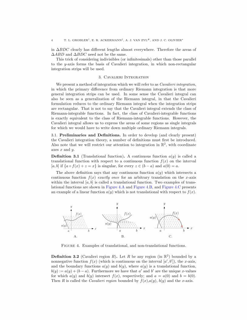
3.1. Preliminaries and Definitions. In order to develop (and clearly present)the Cavalieri integration theory, a number of definitions must first be introduced.Also note that we will restrict our attention to integration in R2, with coordinateaxes x and y.
Definition 3.1 (Translational function). A continuous function a(y) is called atranslational function with respect to a continuous function f(x) on the interval[a, b] if {a ◦ f(x) + z = x} is singular, for every z ∈ (b− a) and a(0) = a.
The above definition says that any continuous function a(y) which intersects acontinuous function f(x) exactly once for an arbitrary translation on the x-axiswithin the interval [a, b] is called a translational function. Two examples of trans-lational functions are shown in Figure 4.A and Figure 4.B, and Figure 4.C presentsan example of a linear function a(y) which is not translational with respect to f(x).
y
f(x)
xa b
a(y)
A.
y
f(x)
xa b
a(y)
B.
y
f(x)
xa b
a(y)
C.
Figure 4. Examples of translational, and non-translational functions.
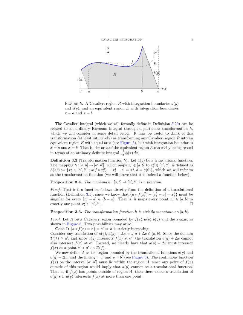
Definition 3.2 (Cavalieri region R). Let R be any region (in R2) bounded by anonnegative function f(x) (which is continuous on the interval [a′, b′]), the x-axis,and the boundary functions a(y) and b(y), where a(y) is a translational function,b(y) := a(y) + (b− a). Furthermore we have that a′ and b′ are the unique x-valuesfor which a(y) and b(y) intersect f(x), respectively; and a = a(0) and b = b(0).Then R is called the Cavalieri region bounded by f(x),a(y), b(y) and the x-axis.
CAVALIERI INTEGRATION 5
y
f
xa b
R
a(y)
b(y)
a′ b′
E
φ
Figure 5. A Cavalieri region R with integration boundaries a(y)and b(y), and an equivalent region E with integration boundariesx = a and x = b.
The Cavalieri integral (which we will formally define in Definition 3.20) can berelated to an ordinary Riemann integral through a particular transformation h,which we will consider in some detail below. It may be useful to think of thistransformation (at least intuitively) as transforming any Cavalieri region R into anequivalent region E with equal area (see Figure 5), but with integration boundariesx = a and x = b. That is, the area of the equivalent region E can easily be expressed
in terms of an ordinary definite integral∫ baφ(x) dx.
Definition 3.3 (Transformation function h). Let a(y) be a translational function.The mapping h : [a, b]→ [a′, b′], which maps x1i ∈ [a, b] to x2i ∈ [a′, b′], is defined ash(x1i ) := {x2i ∈ [a′, b′] : a(f ◦ x2i ) + [x1i − a] = x2i , a = a(0)}, which we will refer toas the transformation function (we will prove that it is indeed a function below).
Proposition 3.4. The mapping h : [a, b]→ [a′, b′] is a function.
Proof. That h is a function follows directly from the definition of a translationalfunction (Definition 3.1), since we know that {a ◦ f(x2i ) + [x1i − a] = x2i } must besingular for every [x1i − a] ∈ (b − a). That is, h maps every point x1i ∈ [a, b] toexactly one point x2i ∈ [a′, b′]. �
Proposition 3.5. The transformation function h is strictly monotone on [a, b].
Proof. Let R be a Cavalieri region bounded by f(x), a(y), b(y) and the x-axis, asshown in Figure 6. Two possibilities may arise.
Case I: {a ◦ f(x) = x} = a′ ⇒ h is strictly increasing:Consider any translation of a(y), a(y) + ∆c, s.t. a+ ∆c ∈ (a, b). Since the domainD(f) ≥ a′, and since a(y) intersects f(x) at a′, the translation a(y) + ∆c cannotalso intersect f(x) at a′. Instead, we clearly have that a(y) + ∆c must intersectf(x) at a point c′ > a′ on D(f).
We now define A as the region bounded by the translational functions a(y) anda(y) + ∆c, and the lines y = a′ and y = b′ (see Figure 6). The continuous functionf(x) on the interval [a′, b′] must lie within the region A, since any point of f(x)outside of this region would imply that a(y) cannot be a translational function.That is, if f(x) has points outside of region A, then there exists a translation ofa(y) s.t. a(y) intersects f(x) at more than one point.

6 T. L. GROBLER†, E. R. ACKERMANN‡, A. J. VAN ZYL#, AND J. C. OLIVIER?
Now consider any translation of a(y), a(y)+∆d, where ∆d > ∆c and ∆d ∈ (a, b].Suppose that a(y) + ∆d induces a point d′, with a′ < d′ < c′. That is, a(y) + ∆dintersects f(x) at some point in region A.
The functions a(y) + ∆c and a(y) + ∆d are continuous on the interval y ∈ [0, γ],where γ := {a ◦ f(x) + ∆d = x} (in fact, any translational function must becontinuous on y ∈ R). Now let Ψ := a(y) + ∆c −
(a(y) + ∆d
), which is again a
continuous function on [0, γ]. Since c < d and c′ > d′ by assumption, it followsthat Ψ(0) < 0 and Ψ(γ) > 0. From the intermediate value theorem it follows thatthere exists a point α ∈ [0, γ] s.t. Ψ(α) = 0. That is, a(α) + ∆c = a(α) + ∆d.But this is impossible, since a(y) + ∆d is a translation of a(y) + ∆c. Thereforec′ = h(c) < h(d) = d′.
Since ∆c is arbitrary and d > c⇒ h(d) > h(c), h is strictly increasing on [a, b].Case II: {a ◦ f(x) = x} = b′ ⇒ h is strictly decreasing:
The second case can be proved in a similar manner as Case I above, in which case his a strictly decreasing function with the order of the induced partition P2 reversed.
Since h is either strictly increasing (Case I) or strictly decreasing (Case II), it isstrictly monotone on [a, b]. �
a′ d′ c′ a
α
c d b′ b
y
x
f(x)
a(y) b(y)
γA
∆c∆d
a(y) + ∆c
a(y) + ∆d
Figure 6. Sketch for the proof of Proposition 3.5.
Proposition 3.6. The transformation function h is continuous on [a, b].
Proof. Choose an arbitrary value x1∗ ∈ [a, b] such that x1∗ = a+c. We can now definea sequence (x1i ) with x1i = x1∗+ 1
i , ∀ i ∈ N. Now (x1i )→ x1∗ as i→∞. The sequence
of functions(a(y) + [x1i − x1∗ + c]
)has x-intercepts equal to (x1i ). The mapping h
now generates a new sequence (x2i ) s.t. ∀ i, x2i = {x2i : a◦f(x2i )+[x1i −x1∗+c] = x2i }.
CAVALIERI INTEGRATION 7
Now taking the limit as i→∞limi→∞
x2i = limi→∞
[a ◦ f(x2i ) + (x1i − x1∗ + c) = x2i ]
= limi→∞
[a ◦ f(x2i ) + (1
i+ c) = x2i ]
= [a ◦ f(x2i ) + ( limi→∞
1
i+ c) = x2i ]
= [a ◦ f(x2i ) + c) = f(x2i )]
= [a(x2i ) + [x1∗ − a]) = f(x2i )]
= x2∗
This shows that x2i → x2∗ as x1i → x1∗ assuming [a ◦ f(x2i ) + [x1∗ − a]) = f(x2i )] hasone unique solution, which must be the case since a(y) is a translational function.The function h must be continuous at x1∗ since x2i → x2∗ as x1i → x1∗. Since x1∗ isarbitrary, h is a continuous function on [a, b]. �
Proposition 3.7. The transformation function h is bijective on [a, b].
Proof. That h is injective on [a, b] follows from the fact that h is strictly monotoneon [a, b] (by Proposition 3.5). Furthermore h is clearly surjective on [a, b], since itis continuous on [a, b] (by Proposition 3.6). Since h is both injective and surjectiveon [a, b], h is also bijective on [a, b]. �
3.2. Derivation of Cavalieri Integration. Since we want to derive the Cavalieriintegral – which uses more general integration strips than the rectangles of theRiemann integral – we first need to formally define valid integration strips.
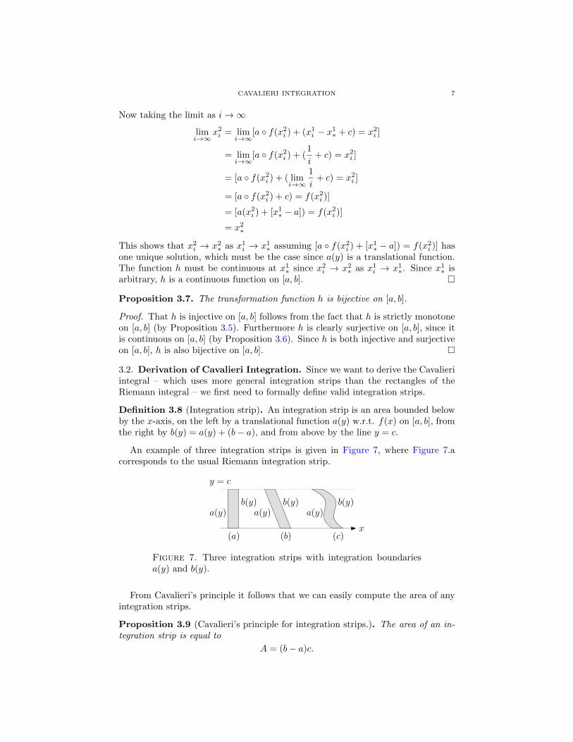
Definition 3.8 (Integration strip). An integration strip is an area bounded belowby the x-axis, on the left by a translational function a(y) w.r.t. f(x) on [a, b], fromthe right by b(y) = a(y) + (b− a), and from above by the line y = c.
An example of three integration strips is given in Figure 7, where Figure 7.acorresponds to the usual Riemann integration strip.
(a) (b) (c)
y = c
x
a(y)b(y)
a(y)b(y)
a(y)b(y)
Figure 7. Three integration strips with integration boundariesa(y) and b(y).
From Cavalieri’s principle it follows that we can easily compute the area of anyintegration strips.
Proposition 3.9 (Cavalieri’s principle for integration strips.). The area of an in-tegration strip is equal to
A = (b− a)c.
8 T. L. GROBLER†, E. R. ACKERMANN‡, A. J. VAN ZYL#, AND J. C. OLIVIER?
Proof. The area of an integration strip can be determined by calculating the areabetween the curves b(y) and a(y) with the definite integral
A =
∫ c
0
b(y)− a(y) dy
=
∫ c
0
(b− a) dy
= (b− a)y∣∣∣c
0
= (b− a)c.
�
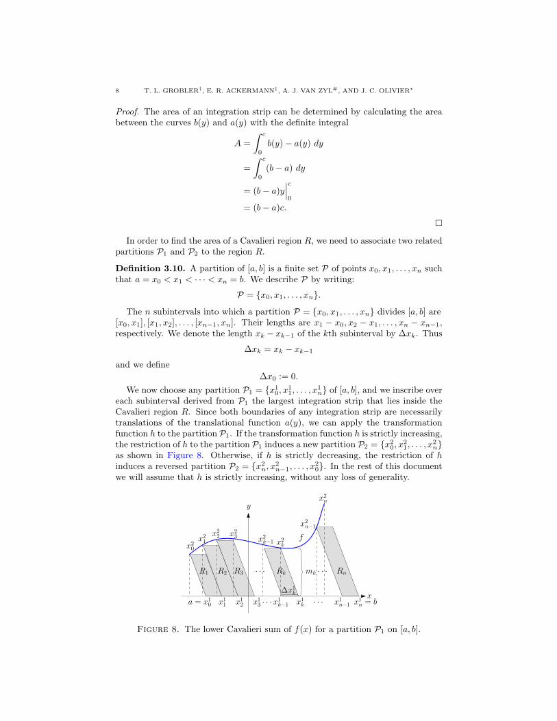
In order to find the area of a Cavalieri region R, we need to associate two relatedpartitions P1 and P2 to the region R.
Definition 3.10. A partition of [a, b] is a finite set P of points x0, x1, . . . , xn suchthat a = x0 < x1 < · · · < xn = b. We describe P by writing:
P = {x0, x1, . . . , xn}.The n subintervals into which a partition P = {x0, x1, . . . , xn} divides [a, b] are
[x0, x1], [x1, x2], . . . , [xn−1, xn]. Their lengths are x1 − x0, x2 − x1, . . . , xn − xn−1,respectively. We denote the length xk − xk−1 of the kth subinterval by ∆xk. Thus
∆xk = xk − xk−1and we define
∆x0 := 0.
We now choose any partition P1 = {x10, x11, . . . , x1n} of [a, b], and we inscribe overeach subinterval derived from P1 the largest integration strip that lies inside theCavalieri region R. Since both boundaries of any integration strip are necessarilytranslations of the translational function a(y), we can apply the transformationfunction h to the partition P1. If the transformation function h is strictly increasing,the restriction of h to the partition P1 induces a new partition P2 = {x20, x21, . . . , x2n}as shown in Figure 8. Otherwise, if h is strictly decreasing, the restriction of hinduces a reversed partition P2 = {x2n, x2n−1, . . . , x20}. In the rest of this documentwe will assume that h is strictly increasing, without any loss of generality.
y
f
xa = x10 x11 x12 x13 · · ·x1k−1 x1k x1n = b
R1 R2 R3 Rk Rn
∆x1k
mk · · ·· · ·
x1n−1· · ·
x20x21
x22 x23 x2k−1 x2k
x2n−1
x2n
Figure 8. The lower Cavalieri sum of f(x) for a partition P1 on [a, b].

CAVALIERI INTEGRATION 9
Since we have assumed that f is continuous and nonnegative on [a′, b′], we knowfrom the Maximum-Minimum theorem that for each k between 1 and n there existsa smallest value mk of f on the kth subinterval [x2k−1, x
2k]. If we choose mk as
the height of the kth integration strip Rk, then Rk will be the largest (tallest)integration strip that can be inscribed in R over [x1k−1, x
1k]. Doing this for each
subinterval, we create n inscribed strips R1, R2, . . . , Rn, all lying inside the regionR. For each k between 1 and n the strip Rk has base [x1k−1, x
1k] with width ∆x1k
and has height mk. Hence the area of Rk is the product mk∆x1k (by Cavalieri’sprinciple). The sum
L(P1, f, h) =
n∑
k=1
mk∆x1k, (lower Cavalieri sum)
where
mk = infxf(x), h(x1i−1) = x2i−1 ≤ x ≤ x2i = h(x1i )
is called the lower Cavalieri sum and should be no larger than the area of R. Thelower Cavalieri sum is represented graphically in Figure 8. Recall that the lowerRiemann sum is defined similarly, that is
L(P, f) =
n∑
k=1
mk∆xk, (lower Riemann sum)
where
mk = infxf(x), xi−1 ≤ x ≤ xi
and P = {x0, x1, . . . , xn} is a partition on [a, b], and the integration strips arerectangular. The lower Riemann sum is represented graphically in Figure 9.
y
f
xa = x0 x1 x2 x3 · · ·xk−1 xk · · ·xn−1 xn = b
R1 R2 R3 Rk Rn
∆xk
mk · · ·· · ·R1
Figure 9. The Lower Riemann Sum of f(x) for a partition P on [a, b].
Irrespective of how we define the area of the Cavalieri region R, this area must beat least as large as the lower Cavalieri sum L(P1, f, h) associated with any partitionP1 of [a, b].
By a procedure similar to the one that involves inscribing integration strips tocompute a lower Cavalieri sum, we can also circumscribe integration strips andcompute an upper Cavalieri sum as shown in Figure 10.
Let P1 = {x10, x11, . . . , x1n} be a given partition of [a, b], and let f be continuousand nonnegative on [a′, b′]. The Maximum-Minimum Theorem implies that for eachk between 1 and n there exists a largest value Mk of f on the kth integration strip

10 T. L. GROBLER†, E. R. ACKERMANN‡, A. J. VAN ZYL#, AND J. C. OLIVIER?
y
f
xa = x10 x11 x12 x13 · · ·x1k−1 x1k x1n = b
R1 R2 R3 Rk Rn
∆x1k
Mk · · ·· · ·
x1n−1· · ·
x20x21
x22 x23 x2k−1 x2k
x2n−1
x2n
Figure 10. The upper Cavalieri sum of f(x) for a partition P1 on [a, b].
Rk, such that Rk will be the smallest possible strip circumscribing the appropriateportion of R. The area of Rk is Mk∆x1k, and the sum
U(P1, f, h) =
n∑
k=1
Mk∆x1k, (upper Cavalieri sum)
where
Mk = supxf(x), h(x1i−1) = x2i−1 ≤ x ≤ x2i = h(x1i )
is called the upper Cavalieri sum of f associated with the partition P1. The up-per Cavalieri sum is represented graphically in Figure 10. Recall that the upperRiemann sum is defined similarly, that is
U(P, f) =
n∑
k=1
Mk∆xk, (upper Riemann sum)
where
Mk = supxf(x), xi−1 ≤ x ≤ xi
and P = {x0, x1, . . . , xn} is a partition on [a, b], and the integration strips arerectangular. The upper Riemann sum is represented graphically in Figure 11.
y
f
xa = x0 x1 x2 x3 · · ·xk−1 xk · · ·xn−1 xn = b
R1 R2 R3 Rk Rn
∆xk
Mk · · ·· · ·
Figure 11. The upper Riemann sum of f(x) for a partition P on [a, b].
Irrespective of how we define the area of the Cavalieri region R, this area mustbe no larger than the upper Cavalieri sum U(P1, f, h) for any partition P1 of [a, b].

CAVALIERI INTEGRATION 11
The assumption that f must be nonnegative on [a′, b′] can now be dropped.Assuming only that f is continuous on [a′, b′], we still define the lower and upperCavalieri sums of f for a partition P1 of [a, b] by
L(P1, f, h) =
n∑
k=1
mk∆x1k
and
U(P1, f, h) =
n∑
k=1
Mk∆x1k,
where for any integer k between 1 and n, mk and Mk are the minimum and maxi-mum values of f on [x2k−1, x
2k], respectively.
Remark 3.11. In the rest of this document we will repeatedly make use of thefollowing notation. We will let f(x) be any continuous function on the interval[a′, b′]. We will also assume that a(y) is some translational function w.r.t. f(x)on the interval [a, b], with which we’ll associate a partition P1. Furthermore, wewill let h denote the transformation function which maps the partition P1 ⊂ [a, b]to the partition P2 ⊂ [a′, b′]. Of course, b(y) must be a particular translation onthe x-axis of a(y), such that b(y) = a(y) + (b − a), where a = a(0) and b = b(0)as defined previously. Finally, we have that a′ and b′ are the unique x-values forwhich a(y) and b(y) intersect f(x), respectively.
Definition 3.12 (Cavalieri sum). For each k ∈ N from 1 to n, let t2k be an arbitrarynumber in [x2k−1, x
2k] ⊆ [a′, b′]. Then the sum
C(P1, f, h) =
n∑
k=1
f(t2k)∆x1k = f(t21)∆x11 + f(t22)∆x12 + · · ·+ f(t2n)∆x1n
is called a Cavalieri sum for f on [a, b].
Recall that a Riemann sum for f on [a, b] is defined similarly, that is
R(P, f) =
n∑
k=1
f(tk)∆xk = f(t1)∆x1 + f(t2)∆x2 + · · ·+ f(tn)∆xn,
where P = {x0, x1, . . . , xn} is any partition of [a, b], and tk is an arbitrary numberin [xk−1, xk] ⊆ [a, b].
Proposition 3.13. The lower Cavalieri sum L(P1, f, h) is equivalent to the lowerRiemann sum L(P1, f ◦ h), that is
(3.1) L(P1, f, h) = L(P1, f ◦ h)
and the upper Cavalieri sum U(P1, f, h) is equivalent to the upper Riemann sumU(P1, f ◦ h):
(3.2) U(P1, f, h) = U(P1, f ◦ h).
Proof. We first consider the lower sums of (3.1). Since the transformation functionh is strictly monotone, continuous and bijective on [a, b] we can choose values of x2ito minimize the value of f in the interval [x2k−1, x
2k] and so minimizing f ◦ h in the
interval [x1k−1, x1k]. The proof of (3.2) is similar. �

12 T. L. GROBLER†, E. R. ACKERMANN‡, A. J. VAN ZYL#, AND J. C. OLIVIER?
Remark 3.14. Proposition 3.13 will be used repeatedly to prove many of theremaining results for Cavalieri integration, since existing results for Riemann sumswill hold trivially for the corresponding Cavalieri sums.
We now give two important results from Riemann integration theory.
Proposition 3.15. Suppose P = {x0, x1, . . . , xn} is a partition of the closed inter-val [a, b], and f a bounded function defined on that interval. Then we have:
• The lower Riemann sum is increasing with respect to refinements of par-titions, i.e. L(P ′, f) ≥ L(P, f) for every refinement P ′ of the partitionP.• The upper Riemann sum is decreasing with respect to refinements of par-
titions, i.e. U(P ′, f) ≤ U(P, f) for every refinement P ′ of the partitionP.• L(P, f) ≤ R(P, f) ≤ U(P, f) for every partition P.
Proof. The proof is taken from [6]. The last statement is simple to prove: takeany partition P = {x0, x1, . . . , xn}. Then inf{f(x), xk−1 ≤ x ≤ xk} ≤ f(tk) ≤sup{f(x), xk−1 ≤ x ≤ xk} where tk is an arbitrary number in [xk−1, xk] and k =1, 2, . . . , n. That immediately implies that L(P, f) ≤ R(P, f) ≤ U(P, f). Theother statements are somewhat trickier. In the case that one additional point t0is added to a particular subinterval [xk−1, xk], let ck = sup f(x) in the interval[xk−1, xk], Ak = sup f(x) in the interval [xk−1, t0], Bk = sup f(x) in the interval[x0, xk]. Then ck ≥ Ak and ck ≥ Bk so that:
ck(xk − xk−1) = ck(xk − t0 + t0 − xk−1)
= ck(xk − t0) + ck(t0 − xk−1)
≥ Bk(xk − t0) +Ak(x0 − tk−1),
which shows that if P = {x0, x1, . . . , xk, xk−1, . . . , xn} and P ′ = {x0, x1, . . . , xk, t0,xk−1, . . . , xn} then U(P ′, f) ≤ U(P, f). The proof for a general refinement P ′ of Puses the same idea plus an elaborate indexing scheme. No more details should benecessary. The proof for the statement regarding the lower sum is analogous. �
Proposition 3.16. Let f be continuous on [a, b]. Then there is a unique numberI satisfying
L(P, f) ≤ I ≤ U(P, f)
for every partition P of [a, b].
Proof. The proof is taken from [2]. From Proposition 3.15 it follows that every lowersum of f on [a, b] is less than or equal to every upper sum. Thus the collectionL of all lower sums is bounded above (by an upper sum) and the collection U ofall upper sums is bounded below (by any lower sum). By the Least Upper BoundAxiom, L has a least upper bound L and U has a greatest lower bound G. Fromour preceding remarks it follows that
L(P, f) ≤ L ≤ G ≤ U(P, f)
for each partition P of [a, b]. Moreover, any number I satisfying
L(P, f) ≤ I ≤ U(P, f)
for each partition P of [a, b] must satisfy
L ≤ I ≤ G

CAVALIERI INTEGRATION 13
since L is the least upper bound of the lower sums and G is the greatest lowerbound of the upper sums. Hence to complete the proof of the theorem it is enoughto prove that L = G. Let ε > 0. Since f is continuous on [a, b], it follows that f isuniformly continuous on [a, b]. Thus there is a δ > 0 such that if x and y are in [a, b]and |x− y| < δ, then |f(x)− f(y)| < ε
b−a . Let P = {x0, x1, . . . , xn} be a partition
of [a, b] such that ∆xk < δ for 1 ≤ k ≤ n, and let Mk and mk be, respectively, thelargest and smallest values of f on [xk−1, xk]. Then
U(P, f)− L(P, f) =
n∑
k=1
Mk∆xk −n∑
k=1
mk∆xk
=
n∑
k=1
(Mk −mk)∆xk
<ε
b− an∑
k=1
∆xk
=ε
b− a (b− a)
= ε.
Since L(P, f) ≤ L ≤ G ≤ U(P, f), it follows that 0 ≤ G−L ≤ U(P, f)−L(P, f) ≤ε. Since ε was arbitrary, we conclude that L = G. �
Definition 3.17 (Definite Riemann integral). Let f be continuous on [a, b]. Thedefinite Riemann integral of f from a to b is the unique number I satisfying
L(P, f) ≤ I ≤ U(P, f)
for every partition P of [a, b]. This integral is denoted by∫ b
a
f(x) dx.
We now state (and prove) the equivalent of Proposition 3.15 for lower and upperCavalieri sums:
Proposition 3.18. We clearly have:
• The lower Cavalieri sum is increasing with respect to refinements of parti-tions, i.e. L(P ′1, f, h) ≥ L(P1, f, h) for every refinement P ′1 of the partitionP1.
• The upper Cavalieri sum is decreasing with respect to refinements of parti-tions, i.e. U(P ′1, f, h) ≤ U(P1, f, h) for every refinement P ′1 of the partitionP1.
• L(P1, f, h) ≤ C(P1, f, h) ≤ U(P1, f, h) for every partition P1.
Proof. The proof follows trivially from Proposition 3.13 and Proposition 3.15 (sinceevery Cavalieri sum corresponds to an equivalent Riemann sum). �
Proposition 3.19. Let f be continuous on [a′, b′]. Then there is a unique numberI satisfying
L(P1, f, h) ≤ I ≤ U(P1, f, h)
for every partition P1 of [a, b].
Proof. The proof follows trivially from Proposition 3.13 and Proposition 3.16. �

14 T. L. GROBLER†, E. R. ACKERMANN‡, A. J. VAN ZYL#, AND J. C. OLIVIER?
We can now finally define the Cavalieri integral:
Definition 3.20 (Definite Cavalieri integral). Let f be continuous on [a′, b′]. Thedefinite Cavalieri integral of f(x) from a(y) to b(y) is the unique number I satisfying
L(P1, f, h) ≤ I ≤ U(P1, f, h)
for every partition P1 of [a, b]. This integral is denoted by∫ b(y)
a(y)
f(x) dx.
Definition 3.21. Let R be any Cavalieri region as given in Definition 3.2 then thearea A of the region R is defined to be
A =
∫ b(y)
a(y)
f(x) dx.
Proposition 3.22. The following Cavalieri and Riemann integrals are equivalent:∫ b(y)
a(y)
f(x) dx =
∫ b
a
f ◦ h(x) dx.
Proof. By noting that L(P1, f ◦ h) = L(P1, f, h) ≤ I ≤ U(P1, f, h) = U(P1, f ◦ h),the proof follows trivially from Proposition 3.13, Proposition 3.16 and Proposi-tion 3.19. �
Theorem 3.23. For any ε > 0 there is a number δ > 0 such that the followingstatement holds: If any subinterval of P1 has length less than δ, and if x2k−1 ≤ t2k ≤x2k for each k between 1 and n, then the associated Cavalieri sum
∑nk=1 f(t2k)∆x1k
satisfies. ∣∣∣∣∣
∫ b(y)
a(y)
f(x) dx−n∑
k=1
f(t2k)∆x1k
∣∣∣∣∣ < ε.
Proof. This proof was adapted from [2]. For any ε > 0 choose δ > 0 such that if xand y are in [a′, b′] then |x− y| < δ, then |f(x)− f(y)| < ε
b′−a′ . If P1 is chosen so
that ∆x1k < δ for each k, then by Proposition 3.19,
U(P1, f, h)− L(P1, f, h) ≤ ε.Moreover, if x2k−1 ≤ t2k ≤ x2k for 1 ≤ k ≤ n, then
mk ≤ f(t2k) ≤Mk.
It follows that
L(P1, f, h) =
n∑
k=1
mk∆x1k ≤n∑
k=1
f(t2k)∆x1k ≤n∑
k=1
Mk∆x1k = U(P1, f, h).
Since
L(P1, f, h) ≤∫ b(y)
a(y)
f(x) dx ≤ U(P1, f, h),
we conclude that ∣∣∣∣∣
∫ b(y)
a(y)
f(x) dx−n∑
k=1
f(t2k)∆x1k
∣∣∣∣∣ < ε.
�

CAVALIERI INTEGRATION 15
By combining Proposition 3.22 and Theorem 3.23 we finally have
∫ b(y)
a(y)
f(x) dx = limn→∞
n∑
k=1
f(t2k)∆x1k
= limn→∞
n∑
k=1
f ◦ h(t1k)∆x1k
=
∫ b
a
f ◦ h(x) dx,
where the last line follows from the well known fact that the limit of a Riemannsum equals the Riemann integral.
3.3. The Cavalieri integral as a Riemann-Stieltjes integral. When evaluat-ing a Cavalieri integral from a(y) to b(y), it may sometimes be more convenient toconsider an equivalent Riemann-Stieltjes integral from a′ to b′ than the ordinaryRiemann integral from a to b.
To transform the Cavalieri integral into an equivalent Riemann-Stieltjes inte-gral, we will make use of the inverse transformation function g := h−1 (which isguaranteed to exist, since h is a bijective function).
Definition 3.24 (Inverse transformation function g). Let a(y) be a translationalfunction. The mapping g : [a′, b′] → [a, b], which maps x2i ∈ [a′, b′] to x1i ∈ [a, b],is defined as g(x2i ) := x2i − a ◦ f(x2i ) + a, which we will refer to as the inversetransformation function.
Proposition 3.25. The following Cavalieri and Riemann-Stieltjes integrals areequivalent:
∫ b(y)
a(y)
f(x) dx =
∫ b′
a′f(x) dg(x).
Proof. From Theorem 3.23 we have
(3.3)
∫ b(y)
a(y)
f(x) dx = limn→∞
n−1∑
i=0
f(x2i )∆x1i .
By noting that ∆x1i = x1i+1 − x1i = g(x2i+1) − g(x2i ), and that g(a′) = a andg(b′) = b, we can re-write (3.3) as
∫ b(y)
a(y)
f(x) dx = limn→∞
n−1∑
i=0
f(x2i )[g(x2i+1)− g(x2i )
],
which we recognize as the Riemann-Stieltjes integral∫ b′a′f(x) dg(x), as required. �
Whenever g is differentiable, we can conveniently express the Cavalieri integralsimply in terms of f(x) and a(y):
∫ b(y)
a(y)
f(x) dx =
∫ b′
a′f(x)
[1− da(y)
dy◦ f(x) · df(x)
dx
]dx.
16 T. L. GROBLER†, E. R. ACKERMANN‡, A. J. VAN ZYL#, AND J. C. OLIVIER?
4. Cavalieri Integration: Worked Examples
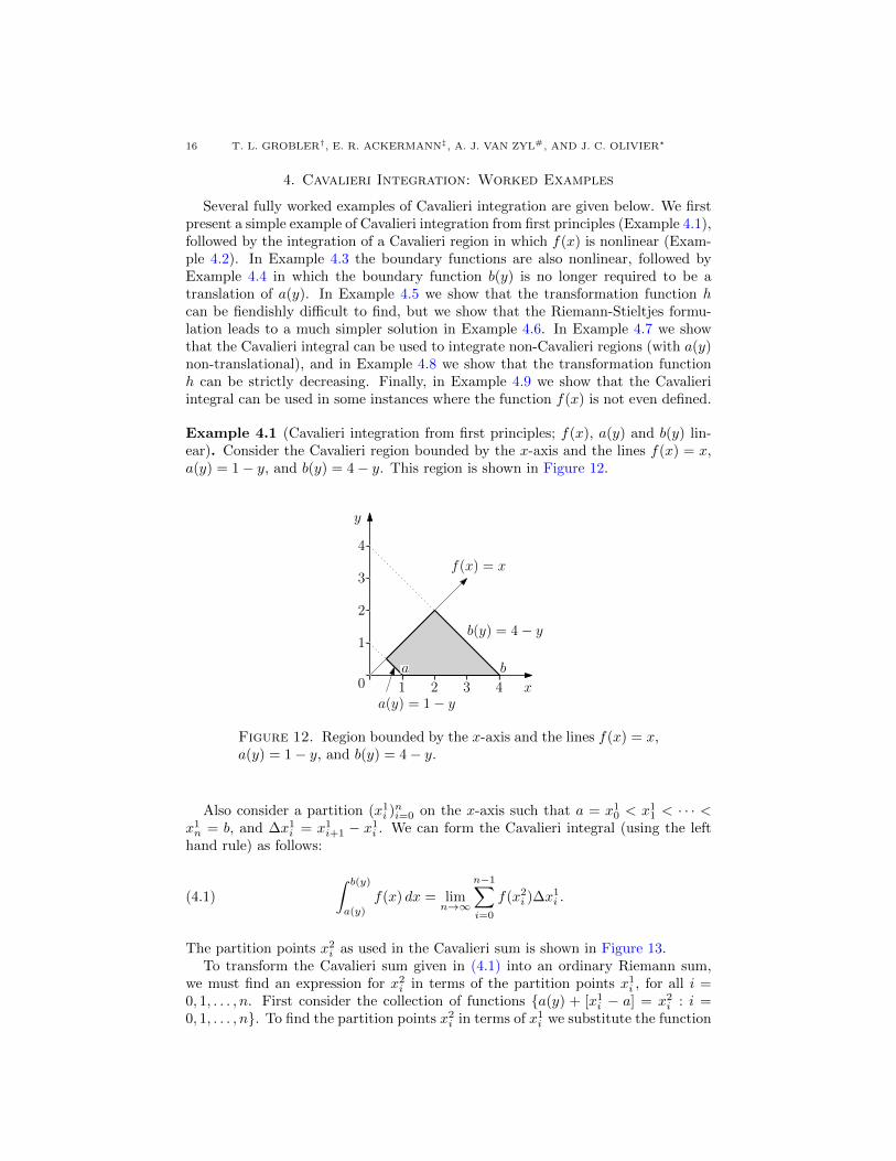
Several fully worked examples of Cavalieri integration are given below. We firstpresent a simple example of Cavalieri integration from first principles (Example 4.1),followed by the integration of a Cavalieri region in which f(x) is nonlinear (Exam-ple 4.2). In Example 4.3 the boundary functions are also nonlinear, followed byExample 4.4 in which the boundary function b(y) is no longer required to be atranslation of a(y). In Example 4.5 we show that the transformation function hcan be fiendishly difficult to find, but we show that the Riemann-Stieltjes formu-lation leads to a much simpler solution in Example 4.6. In Example 4.7 we showthat the Cavalieri integral can be used to integrate non-Cavalieri regions (with a(y)non-translational), and in Example 4.8 we show that the transformation functionh can be strictly decreasing. Finally, in Example 4.9 we show that the Cavalieriintegral can be used in some instances where the function f(x) is not even defined.
Example 4.1 (Cavalieri integration from first principles; f(x), a(y) and b(y) lin-ear). Consider the Cavalieri region bounded by the x-axis and the lines f(x) = x,a(y) = 1− y, and b(y) = 4− y. This region is shown in Figure 12.
x
y
f(x) = x
b(y) = 4− y
a(y) = 1− y
4
2
21 3 40
1
3
a b
Figure 12. Region bounded by the x-axis and the lines f(x) = x,a(y) = 1− y, and b(y) = 4− y.
Also consider a partition (x1i )ni=0 on the x-axis such that a = x10 < x11 < · · · <
x1n = b, and ∆x1i = x1i+1 − x1i . We can form the Cavalieri integral (using the lefthand rule) as follows:
(4.1)
∫ b(y)
a(y)
f(x) dx = limn→∞
n−1∑
i=0
f(x2i )∆x1i .
The partition points x2i as used in the Cavalieri sum is shown in Figure 13.To transform the Cavalieri sum given in (4.1) into an ordinary Riemann sum,
we must find an expression for x2i in terms of the partition points x1i , for all i =0, 1, . . . , n. First consider the collection of functions {a(y) + [x1i − a] = x2i : i =0, 1, . . . , n}. To find the partition points x2i in terms of x1i we substitute the function

CAVALIERI INTEGRATION 17
x
y
4
1
21 3 40
x10 x11 x12 x13
x20
x21
x22
x232
3
a(y) + [x13 − 1]
a(y) + [x12 − 1]
a(y) + [x11 − 1]
a(y)
∆x12
x
y
4
2
21 3 40
1
3
(a) n = 3 (b) n = 12
Figure 13. Partition points x2i as used in the Cavalieri sum.
f(x2i ) for y to obtain:
a ◦ f(x2i ) + [x1i − 1] = x2i
−x2i + x1i = x2i
x2i =x1i2,
so that we have the general expression x2i = h(x1i ), with h(x) = x/2.Finally this allows us to rewrite the Cavalieri integral from (4.1) as an equivalent
Riemann integral:
∫ b(y)
a(y)
f(x) dx = limn→∞
n−1∑
i=0
f(x2i )∆x1i
= limn→∞
n−1∑
i=0
f ◦ h(x1i )∆x1i
=
∫ b
a
f ◦ h(x) dx.(4.2)
Evaluating the Riemann integral of (4.2) with a = 1 and b = 4 we obtain
∫ b(y)
a(y)
f(x) dx =
∫ b
a
f ◦ h(x) dx
=1
2
∫ 4
1
x dx
=1
4x2∣∣∣4
1
= 3.75,

18 T. L. GROBLER†, E. R. ACKERMANN‡, A. J. VAN ZYL#, AND J. C. OLIVIER?
which we can quickly verify to be correct by evaluating the area of the region shownin Figure 12 with ordinary Riemann integration:
∫ 2
0
x dx+
∫ 4
2
4− x dx−∫ 1
2
0
x dx−∫ 1
12
1− x dx = 3.75
=
∫ b(y)
a(y)
f(x) dx.
Example 4.2 (Cavalieri integration; f(x) nonlinear). Consider the Cavalieri regionbounded by the x-axis and the functions f(x) = x2, a(y) = 1− y, and b(y) = 4− y.This region is shown in Figure 14, along with the strips of integration.
0 1 2 3 4
1
2
3
4f(x) = x2
a(y) = 1− y
b(y) = 4− y
x
y
Figure 14. Region bounded by the x-axis and the functionsf(x) = x2, a(y) = 1− y, and b(y) = 4− y.
The area of this region can be calculated with the Cavalieri integral
(4.3)
∫ b(y)
a(y)
f(x) dx =
∫ b
a
f ◦ h(x) dx.
To evaluate (4.3) we first need to find h using Definition 3.3:
a ◦ f(x2i ) + [x1i − 1] = x2i
−(x2i )2 + 1 + x1i − 1 = x2i
(x2i )2 + x2i − x1i = 0
x2i =1
2
(√4x1i + 1− 1
)
= h(x1i ).
CAVALIERI INTEGRATION 19
We can now calculate (4.3) with h(x) = 12 (√
4x+ 1− 1) as follows
∫ b(y)
a(y)
f(x) dx =
∫ b
a
f ◦ h(x) dx
=1
4
∫ 4
1
(√
4x+ 1− 1)2 dx
= − 1
96(4x+ 1)(−12x+ 8
√4x+ 1− 9)
∣∣∣4
1
= 9 +1
12(5√
5− 17√
17)
≈ 4.09063.
One can also compute the area under consideration (see Figure 14) using ordinaryRiemann integration:
∫ 12 (√17−1)
0
x2 dx+
∫ 4
12 (√17−1)
4− x dx
−∫ 1
2 (√5−1)
0
x2 dx−∫ 1
12 (√5−1)
1− x dx ≈ 4.09063
≈∫ b(y)
a(y)
f(x) dx.
Example 4.3 (Cavalieri integration; f(x), a(y) and b(y) nonlinear). Consider theCavalieri region bounded by the x-axis and the functions f(x) = x2, a(y) = 2−√y,and b(y) = 4 − √y. This region is shown in Figure 15, along with the strips ofintegration.
f(x) = x2 b(y) = 4−√y
a(y) = 2−√y21 3 4
1
2
3
4
0x
y
a b
Figure 15. Region bounded by the x-axis and the functionsf(x) = x2, a(y) = 2−√y, and b(y) = 4−√y.
The area of this region can be calculated with the Cavalieri integral
(4.4)
∫ b(y)
a(y)
f(x) dx =
∫ b
a
f ◦ h(x) dx.
20 T. L. GROBLER†, E. R. ACKERMANN‡, A. J. VAN ZYL#, AND J. C. OLIVIER?
To evaluate (4.4) we first need to find h:
a ◦ f(x2i ) + [x1i − 2] = x2i
−x2i + 2 + x1i − 2 = x2i
x2i =1
2x1i
= h(x1i ).
We can now calculate (4.4) with h(x) = x/2 as follows
∫ b(y)
a(y)
f(x) dx =
∫ b
a
f ◦ h(x) dx
=1
4
∫ 4
2
x2 dx
=1
12x3∣∣∣4
2
=14
3.
We can once again verify our answer above by computing the area of the regionshown in Figure 15 with ordinary Riemann integration:
∫ 2
0
x2 dx+
∫ 4
2
(4− x)2 dx−∫ 1
0
x2 dx−∫ 2
1
(2− x)2 dx =14
3
=
∫ b(y)
a(y)
f(x)dx.
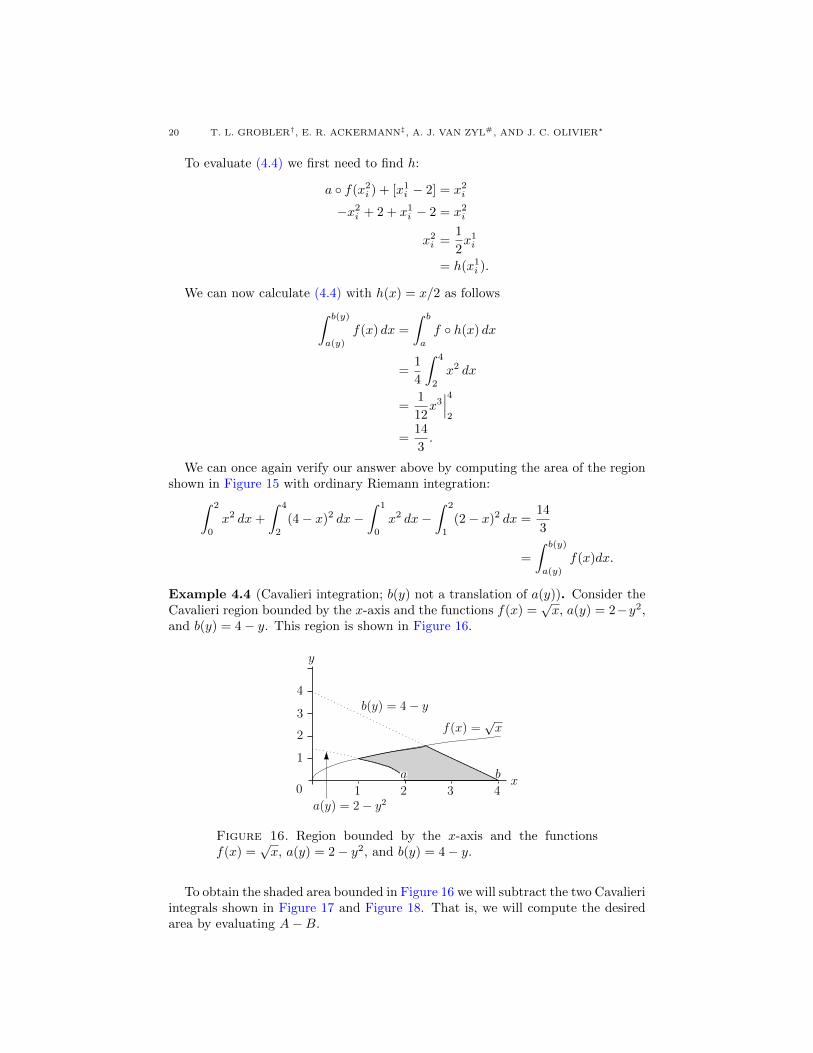
Example 4.4 (Cavalieri integration; b(y) not a translation of a(y)). Consider theCavalieri region bounded by the x-axis and the functions f(x) =
√x, a(y) = 2−y2,
and b(y) = 4− y. This region is shown in Figure 16.
f(x) =√x
b(y) = 4− y
a(y) = 2− y221 3 4
1
2
3
4
0x
y
ba
Figure 16. Region bounded by the x-axis and the functionsf(x) =
√x, a(y) = 2− y2, and b(y) = 4− y.
To obtain the shaded area bounded in Figure 16 we will subtract the two Cavalieriintegrals shown in Figure 17 and Figure 18. That is, we will compute the desiredarea by evaluating A−B.

CAVALIERI INTEGRATION 21
f(x) =√x
21 3 4
1
2
3
4
0x
y
baA
Figure 17. Region bounded by the x-axis and the functionsf(x) =
√x and b(y) = 4− y.
The area of A can be calculated with the Cavalieri integral
(4.5)
∫ b(y)
−yf(x) dx =
∫ b
0
f ◦ h1(x) dx.
To evaluate (4.5) we first need to find h1:
−f(x2i ) + x1i = x2i
−√x2i + x1i = x2i
√x2i + x2i − x1i = 0
x2i =(x1i +
1
2
)− 1
2
√4x1i + 1
= h1(x1i ).
We can now calculate (4.5) with h1(x) = (x+ 0.5)− 0.5√
4x+ 1 as follows:∫ b(y)
−yf(x) dx =
∫ b
0
f ◦ h1(x) dx
=
∫ 4
0
√(x+ 0.5)− 0.5
√4x+ 1 dx
=1
12(4x+ 1)
32 − 1
2x− 1
8
∣∣∣∣∣
4
0
≈ 3.75773.
The area of B can be calculated with the Cavalieri integral (see Figure 18)
(4.6)
∫ a(y)
−y2f(x) dx =
∫ a
0
f ◦ h2(x) dx.
To evaluate (4.6) we first need to find h2:
−(f(x2i ))2 + x1i = x2i
−x2i + x1i = x2i
x2i =1
2x1i
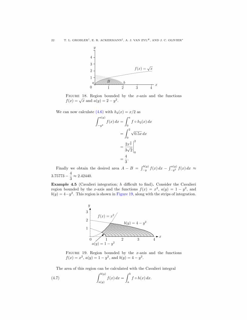
22 T. L. GROBLER†, E. R. ACKERMANN‡, A. J. VAN ZYL#, AND J. C. OLIVIER?
f(x) =√x
21 3 4
1
2
3
4
0x
y
ba B
Figure 18. Region bounded by the x-axis and the functionsf(x) =
√x and a(y) = 2− y2.
We can now calculate (4.6) with h2(x) = x/2 as∫ a(y)
−y2f(x) dx =
∫ a
0
f ◦ h2(x) dx
=
∫ 2
0
√0.5x dx
=2x
32
3√
2
∣∣∣∣∣
2
0
=4
3.
Finally we obtain the desired area A − B =∫ b(y)−y f(x) dx −
∫ a(y)−y2 f(x) dx ≈
3.75773− 4
3≈ 2.42440.
Example 4.5 (Cavalieri integration; h difficult to find). Consider the Cavalieriregion bounded by the x-axis and the functions f(x) = x2, a(y) = 1 − y2, andb(y) = 4−y2. This region is shown in Figure 19, along with the strips of integration.
0 1 2 3 4
1
2
3f(x) = x2
a(y) = 1− y2
b(y) = 4− y2
x
y
Figure 19. Region bounded by the x-axis and the functionsf(x) = x2, a(y) = 1− y2, and b(y) = 4− y2.
The area of this region can be calculated with the Cavalieri integral
(4.7)
∫ b(y)
a(y)
f(x) dx =
∫ b
a
f ◦ h(x) dx.

CAVALIERI INTEGRATION 23
To evaluate (4.7) we first need to find h:
a ◦ f(x2i ) + [x1i − 1] = x2i
−(x2i )4 + 1 + x1i − 2 = x2i
(x2i )4 + x2i − x1i = 0.
Solving for x2i in terms of x1i produces h(x) which is equal to:
(4.8) h(x) =1
2
√2√G(x)
−G(x)− 1
2
√G(x)
with
G(x) =3√√
3.√
256x3 + 27 + 93√
2.323
−4 3
√23x
3√√
3.√
256x3 + 27 + 9.
We can now calculate (4.7) with h(x) given by (4.8) as follows:
∫ b(y)
a(y)
f(x) dx =
∫ b
a
f ◦ h(x) dx
=
∫ 4
1
(1
2
√2√G(x)
−G(x)− 1
2
√G(x)
)2
dx
≈ 3.46649,
which we will once again verify by using ordinary Riemann integration:∫ 1.28378
0
x2 dx+
∫ 4
1.28378
√4− x dx
−∫ 0.724492
0
x2 dx−∫ 1
0.724492
√1− x dx ≈ 3.46649
≈∫ b(y)
a(y)
f(x) dx.
Example 4.6 (Riemann-Stieltjes formulation). Consider the Cavalieri region boundedby the x-axis and the functions f(x) = x2, a(y) = 1 − y, and b(y) = 4 − y. Thisregion is shown in Figure 20, along with the strips of integration. Note that this isthe same region as studied in Example 4.2. We will show that the Riemann-Stieltjesformulation is considerably simpler than the direct method in which we need to findh explicitly.
The area of this region can be calculated with the Cavalieri integral
(4.9)
∫ b(y)
a(y)
f(x) dx =
∫ b′
a′f(x) dg(x).
To evaluate (4.9) we first need to find g using Definition 3.24:
x1i = x2i − a ◦ f(x2i ) + 1
= (x2i )2 + x2i
= g(x2i ).
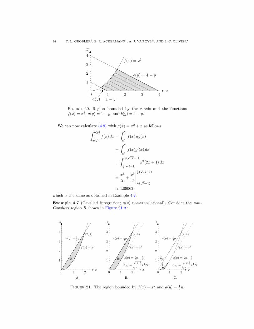
24 T. L. GROBLER†, E. R. ACKERMANN‡, A. J. VAN ZYL#, AND J. C. OLIVIER?
0 1 2 3 4
1
2
3
4f(x) = x2
a(y) = 1− y
b(y) = 4− y
x
y
Figure 20. Region bounded by the x-axis and the functionsf(x) = x2, a(y) = 1− y, and b(y) = 4− y.
We can now calculate (4.9) with g(x) = x2 + x as follows∫ b(y)
a(y)
f(x) dx =
∫ b′
a′f(x) dg(x)
=
∫ b′
a′f(x)g′(x) dx
=
∫ 12 (√17−1)
12 (√5−1)
x2(2x+ 1) dx
=x4
2+x3
3
∣∣∣∣∣
12 (√17−1)
12 (√5−1)
≈ 4.09063,
which is the same as obtained in Example 4.2.
Example 4.7 (Cavalieri integration; a(y) non-translational). Consider the non-Cavalieri region R shown in Figure 21.A:
0 1 2
1
2
3
4(2, 4)
a(y) = 12y
f(x) = x2
x
y
R
A.
0 1 2
1
2
3
4(2, 4)
a(y) = 12y
f(x) = x2
x
y
b(y) = 12y +
12
AR1=∫ 1
2y+12
12y
x2dx
R1
B.
0 1 2
1
2
3
4(2, 4)
a(y) = 12y
f(x) = x2
x
y
b(y) = 12y +
12
AR2=∫ 1
2y+12
12y
x2dx
R2
C.
Figure 21. The region bounded by f(x) = x2 and a(y) = 12y.

CAVALIERI INTEGRATION 25
The area of this region can be calculated with the double integral:
AR =
∫ 4
0
∫ √y12y
1 dx dy
=
∫ 4
0
x∣∣∣√y
12ydy
=
∫ 4
0
√y − 1
2y dy
=2
3y
32 − 1
4y2∣∣∣4
0
=4
3,
and also with the integral:
AR =
∫ 2
0
2x− x2 dx
= x2 − 1
3x3∣∣∣2
0
=4
3.
We can also calculate the area AR with the difference between two Cavalieriintegrals. The two areas being subtracted are shown in Figure 21.B and Figure 21.C.
AR = AR1 −AR2
=
∫ 12y+
12
12y
x2 −∫ 1
2y+12
12y
x2
=
∫ 12
0
f ◦ h1(x) dx−∫ 1
2
0
f ◦ h2(x) dx
=
∫ 12
0
(1 +√
1− 2x)2dx−
∫ 12
0
(1−√
1− 2x)2dx
=4
3.
Example 4.8 (Cavalieri integration; h strictly decreasing). Consider the Cavalieriregion bounded by the x-axis and the functions f(x) = 3 − 2x, a(y) = 2 − y, andb(y) = 3− y. This region is shown in Figure 22.
The area of this region can be calculated with the Cavalieri integral
(4.10)
∫ b(y)
a(y)
f(x) dx =
∫ b
a
f ◦ h(x) dx.
To evaluate (4.10) we first need to find h:
a ◦ f(x2i ) + [x1i − 2] = x2i
⇒ x2i = 3− x1i ,
so that h(x) = 3− x.
26 T. L. GROBLER†, E. R. ACKERMANN‡, A. J. VAN ZYL#, AND J. C. OLIVIER?
0 1 2 3
1
2
3
f(x) = 3− 2x
a(y) = 2− y
b(y) = 3− y
x
y
Figure 22. Region bounded by the x-axis and the functionsf(x) = 3− 2x, a(y) = 2− y, and b(y) = 3− y.
We can now calculate (4.10) as follows∫ b(y)
a(y)
f(x) dx =
∫ b
a
f ◦ h(x) dx
=
∫ 3
2
2x− 3 dx
= x2∣∣∣3
2− 3x
∣∣∣3
2
= 2.
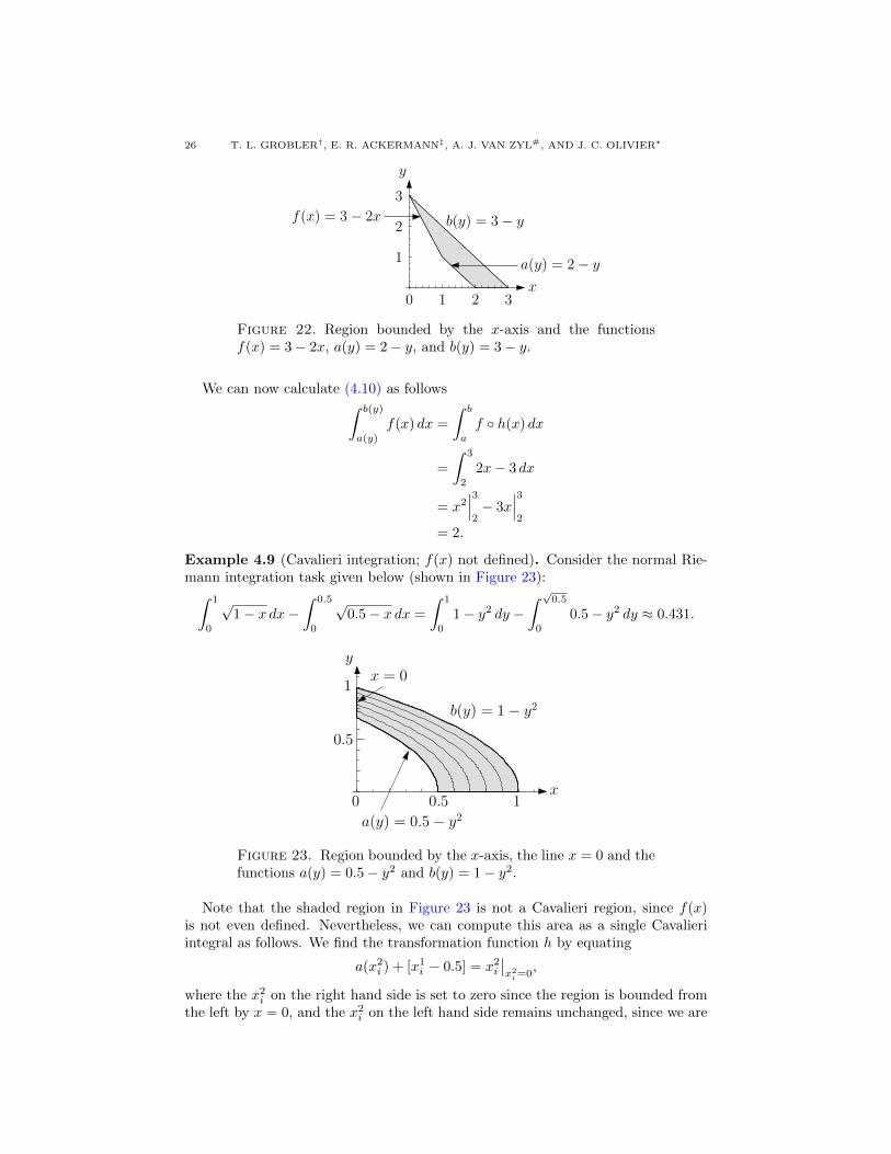
Example 4.9 (Cavalieri integration; f(x) not defined). Consider the normal Rie-mann integration task given below (shown in Figure 23):∫ 1
0
√1− x dx−
∫ 0.5
0
√0.5− x dx =
∫ 1
0
1− y2 dy −∫ √0.5
0
0.5− y2 dy ≈ 0.431.
0 0.5 1
1
0.5
b(y) = 1− y2
a(y) = 0.5− y2
x
yx = 0
Figure 23. Region bounded by the x-axis, the line x = 0 and thefunctions a(y) = 0.5− y2 and b(y) = 1− y2.
Note that the shaded region in Figure 23 is not a Cavalieri region, since f(x)is not even defined. Nevertheless, we can compute this area as a single Cavalieriintegral as follows. We find the transformation function h by equating
a(x2i ) + [x1i − 0.5] = x2i∣∣x2i=0
,
where the x2i on the right hand side is set to zero since the region is bounded fromthe left by x = 0, and the x2i on the left hand side remains unchanged, since we are

CAVALIERI INTEGRATION 27
really interested in the y-intercepts of each translation of a(y). Therefore we find
x2i = h(x1i ) =√x1i ,
so that we can compute the shaded area as∫ b(y)
a(y)
(x = 0) dx =
∫ b
a
h(x) dx
=
∫ 1
0.5
√x dx
≈ 0.431.
5. Conclusion
We have presented a novel integral∫ b(y)a(y)
f(x) dx in which non-rectangular inte-
gration strips were used. We also presented two methods of evaluating Cavalieriintegrals by establishing the following relationships between Cavalieri, Riemannand Riemann-Stieltjes integrals:
∫ b(y)
a(y)
f(x) dx =
∫ b
a
f ◦ h(x) dx =
∫ b′
a′f(x) dg(x),
which is equivalent to noting that
Area A = Area B = Area C,
as shown in Figure 24.
∆x ∆x
f f ◦ h
fg′
A B
C
area A = area B = area C
a b a bb′a′
a′ b′
Figure 24. Relationships between Cavalieri (region A), Riemann(region B) and Riemann-Stieltjes (region C) integrals.
The reason for calling∫ b(y)a(y)
f(x) dx the Cavalieri integral should now become
transparently clear: the area of region B is equal to the area of region A by Cava-lieri’s principle.

28 T. L. GROBLER†, E. R. ACKERMANN‡, A. J. VAN ZYL#, AND J. C. OLIVIER?
References
[1] K. Andersen, “Cavalieri’s Method of Indivisibles,” Arch. Hist. Exact Sci., vol. 31, no. 4,pp. 291–367, 1985.
[2] R. Ellis and D. Gulick, Calculus with analytic geometry. (4th ed.), Harcourt Brace Jovanovich
College Publisher, Orlando, Florida, 1990, pp. A-12–A-13.[3] H. Eves, “Two Surprising Theorems on Cavalieri Congruence,” College Math. J., vol. 22,
no. 2, pp. 118–124, 1991.
[4] J. J. O’ Connor and E. F. Robertson, Antiphon the Sophist, 1999. [Online]. Available: http://www-history.mcs.st-andrews.ac.uk/Biographies/Antiphon.html
[5] A. A. Ruffa, “The generalized method of exhaustion,” Int. J. Math. Math. Sci., vol. 31, no. 6,pp. 345–351, 2002.
[6] B. G. Wachsmuth, Interactive Real Analysis, 2007. [Online]. Available: http://www.mathcs.org/analysis/reals/integ/proofs/rsums.html
† Department of Electrical, Electronic and Computer Engineering, University ofPretoria, and Defence, Peace, Safety and Security; Council for Scientific and Indus-
trial Research, Pretoria, South Africa.
E-mail address: [email protected]
‡ Department of Electrical, Electronic and Computer Engineering, University of
Pretoria, and Defence, Peace, Safety and Security; Council for Scientific and Indus-trial Research, Pretoria, South Africa.
E-mail address: [email protected]
# Department of Mathematics and Applied Mathematics, University of Pretoria,
Pretoria, South Africa.
E-mail address: [email protected]
? Department of Electrical, Electronic and Computer Engineering, University of
Pretoria, and Defence, Peace, Safety and Security; Council for Scientific and Indus-trial Research, Pretoria, South Africa.
E-mail address: [email protected]